ANL - HEP - PR - 96 -52

hep - ph 9607

1 July 1996

FROISSART BOUNDARY
FOR DEEP INELASTIC STRUCTURE
FUNCTIONS
A. L. Ayala F${}^{\underline{o}}$ ${}^{a)\,b)}$^∗ , M. B. Gay Ducati ^a)∗∗
and

E. M. Levin ${}^{c)\,d)}{}^{\dagger}$

^a)Instituto de Física, Univ. Federal do Rio Grande do Sul
Caixa Postal 15051, 91501-970 Porto Alegre, RS, BRAZIL
^b)Instituto de Física e Matemática, Univ. Federal de Pelotas
Campus Universitário, Caixa Postal 354, 96010-900, Pelotas, RS, BRAZIL
^c) Physics Division, Argonne National Laboratory

Argonne, IL 60439, USA
^d) Theory Department, Petersburg Nuclear Physics Institute
188350, Gatchina, St. Petersburg, RUSSIA

Abstract: In this letter we derive the Froissart boundary in QCD for the deep inelastic structure function in low $x$ kinematic region. We show that the comparison of the Froissart boundary with the new HERA experimental data gives rise to a challenge for QCD to explain the matching between the deep inelastic scattering and real photoproduction process.

1 Introduction.

The new HERA data [1] show the steep $x$-dependence of the total cross section in the deep inelastic scattering ( DIS ) of virtual photon off a proton ( $\sigma_{tot}(\gamma^{*}p)$ ). Approximately, $\sigma(\gamma^{*}p)\,\propto\,x^{-0.2}$ at small $x$ ( $10^{-2}\,\leq\,x\,\leq\,10^{-5}$ ). Surprisingly, this energy rise holds at rather small photon virtualities ( $Q^{2}\,\approx\,1-2GeV^{2}$ ). At first sight it means that in HERA kinematic region we still have sufficiently diluted parton cascade and the parton-parton interaction which shall stop the increase of the parton density [2] is still rather small. On the other hand, the probability of the parton - parton interaction [2] ($\kappa$ ) is equal to

$$\kappa\,=\,xG(x,Q^{2})\frac{\sigma(GG)}{\pi R^{2}}\,=\,\frac{N_{c}\alpha_{\rm S}\pi}{2Q^{2}R^{2}}\,xG(x,Q^{2})\,\,,$$ (1)

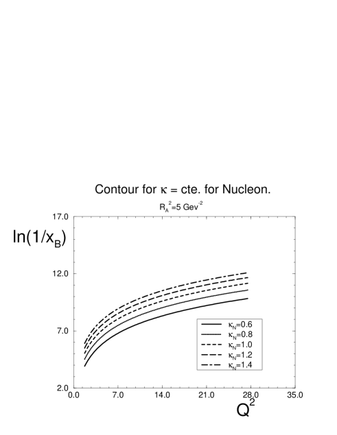
Figure 1: Contour plot for $\kappa$ for $R^{2}=\,5Gev^{-2}$.

where $xG(x,Q^{2})$ is the number of partons ( gluons) in the parton cascade, $\sigma$ is the cross section of parton-parton interaction and $R^{2}$ is the size of a hadron. The numerical factor in Eq. (1) has been evaluated by Mueller and Qiu [3] and has been confirmed in many further publications [4]. Fig.1 shows the contour plot for $\kappa$ using the GRV parameterization [5] for the gluon structure function and the value of $R^{2}=5GeV^{-2}$. We will argue a bit later that this value of $R^{2}$ follows directly from HERA measurement of the diffraction production of J/$\Psi$ meson [6]. One can see that $\kappa$ reaches $\kappa$ = 1 at HERA kinematic region, meaning shadowing corrections take place. Therefore, the situation looks very controversial.

The goal of this letter is to derive the Froissart boundary for the deep inelastic structure function. This should clarify when the shadowing corrections to the deep inelastic process become important. Some attempts have been made to derive the geometrical limit ( the Froissart boundary) during the last three decades ( see Refs.[7] [8] and lectures [9] for update review on the subject) assuming that a target is black for the dominant hadronic component in the wave function of the virtual photon. We derive the Froissart boundary for the deep inelastic processes assuming the GLAP evolution equation for the parton densities and the colour dipole picture of interaction proposed by A. Mueller [10] [11] ( see also Refs.[12] [13] [14] where many of aspects of the Mueller approach have been foreseen).

2 Unitarity constraint for DIS.

2.1 $s$ - channel unitarity ( general formulae).

The unitarity constraint can easily be derived considering the DIS in the frame where a target is at rest. In this frame the virtual photon at high energy ( small $x$ ) decays in quark - antiquark ( $\bar{q}q$ ) pair long before the interaction with the target. The $\bar{q}q$ system traverses the target with fixed transverse distance $r_{\perp}$ between quark and antiquark [12] [10]. Indeed, $r_{\perp}$ can vary by amount $\Delta r_{\perp}\,\propto\,R\,\frac{k_{\perp}}{Q_{0}}$, where $Q_{0}$ denotes the energy of the $\bar{q}q$ pair or the virtual photon in the target rest frame, $R$ is the size of the target, and the quark momentum is $k_{\perp}\,\propto\,\frac{1}{r_{\perp}}$ ( see Fig.2 ). Therefore

$$\Delta r_{\perp}\,\,\propto\,\,R\,\frac{k_{\perp}}{Q_{0}}\,\,\ll\,\,r_{\perp}\,\,,$$ (2)

which in terms of $x$ has the following form:

$$x\,\,\ll\,\,\frac{1}{2mR}\,\,.$$ (3)

Figure 2: DIS in the target rest frame.

The cross section for the DIS can be written in the form:

$$\sigma(\gamma^{*}p)\,\,=\,\,\int^{1}_{0}\,dz\,\int\,d^{2}r_{\perp}\,\Psi(z,r_{\perp})\,\sigma_{tot}(zQ_{0},r^{2}_{\perp})\,\Psi^{*}(z,r_{\perp})\,\,,$$ (4)

cross section for $\bar{q}q$ interaction with the target, $z$ is the fraction of energy of the photon ( $Q_{0}$ ) carried by quark and $r_{\perp}$ is the transverse separation between quark and antiquark. $\Psi$ is the wave function of $\bar{q}q$ - pair in the virtual photon. This wave function is well known [10] [14] and $|\Psi_{T}|^{2}$ for transverse polarized photon and for massless quarks is equal to

$$|\Psi_{T}|^{2}\,\,=\,\,\frac{\alpha_{\rm S}^{em}N_{c}}{2\pi^{2}}\,\sum^{N_{f}}_{1}\,Z^{2}_{f}\,[\,z^{2}+(1-z)^{2}\,]\,{\bar{Q}}^{2}\,K^{2}_{1}(\,\bar{Q}\,r_{\perp}\,)\,\,,$$

where $K_{1}$ is the modified Bessel function, ${\bar{Q}}^{2}\,=\,z(1-z)Q^{2}$ , $N_{f}$ is the number of massless quarks and $Z_{f}$ is the fraction of the charge carried by the quark.

The main contribution in Eq. (4) (see Ref.[10] for details ), which corresponds to the GLAP evolution, comes from the region $\bar{Q}\,r_{\perp}\,\leq\,1$ and $z(1-z)\,\leq\,\frac{1}{Q^{2}\,r^{2}_{\perp}}\,\leq\,\frac{1}{4}$. In this case the integral over $z$ can be taken explicitly. Since $z\,\,\ll\,\,1$, it can be reduced to the integral

$$\int^{1}_{0}dz{\bar{Q}}^{2}\,K^{2}_{1}(\bar{Q}\,r_{\perp})\,\,\rightarrow\,\,2\,Q^{2}\int^{\infty}_{0}\,z\,dz\,K^{2}_{1}(\sqrt{z}\,Q\,r_{\perp})\,=\,\frac{8}{3\,Q^{2}\,r^{4}_{\perp}}\,\,,$$ (5)

with $Q^{2}\,r^{2}_{\perp}\,\geq\,4$. Finally, we have

$$\sigma(\gamma^{*}p)\,\,=\,\,\frac{4\,N_{c}\,\alpha_{\rm S}^{em}}{3\,\pi}\,\sum^{N_{f}}_{1}\,Z^{2}_{f}\,\,\frac{1}{Q^{2}}\,\int^{\infty}_{\frac{4}{Q^{2}}}\,\,\frac{dr^{2}_{\perp}}{r^{4}_{\perp}}\,\sigma_{tot}(\frac{Q_{0}}{Q^{2}\,r^{2}_{\perp}},r^{2}_{\perp})\,\,.$$ (6)

At high energies ( low $x$ ) we can restrict ourselves by summing only $(\alpha_{\rm S}\ln(1/x))^{n}$ contribution in each $\alpha_{\rm S}^{n}$ order of perturbative QCD ( so called leading log(1/$x$) approximation (LL($x$)A)). In the framework of the LL(x)A we can safely replace the argument of $\sigma$ in Eq. (6) by $x$. Taking into account the relation between the cross section and $F_{2}$ structure function, namely $\sigma_{tot}(\gamma^{*}p)\,=\,\frac{4\pi^{2}\alpha_{\rm S}}{Q^{2}}F_{2}(x,Q^{2})$, the final formula has a form [10]:

$$F_{2}(x,Q^{2})\,\,=\,\,\frac{N_{c}}{12\pi^{3}}\,\sum^{N_{f}}_{1}\,Z^{2}_{f}\,\,\int^{\infty}_{\frac{1}{Q^{2}}}\,\,\frac{dr^{2}_{\perp}}{r^{4}_{\perp}}\,\sigma_{tot}(x,\frac{r^{2}_{\perp}}{4})\,\,.$$ (7)

The total cross section for $\bar{q}q$ scattering can be written as

$$\sigma_{tot}(x,\frac{r^{2}_{\perp}}{4})\,\,=\,\,2\,\int\,d^{2}b_{\perp}\,Im\,a(x,r_{\perp},b_{\perp})\,\,,$$ (8)

where $a$ is the amplitude for elastic scattering of $\bar{q}q$ in impact parameter ($b_{\perp}$) space which is defined as

$$a(x,r_{\perp},b_{\perp})\,\,=\,\,\frac{1}{2\pi}\,\int\,d^{2}q_{\perp}\,e^{-\,i\,{\vec{q}}_{\perp}\cdot{\vec{b}}_{\perp}}\,f(x,r_{\perp},t=-q^{2}_{\perp})\,\,,$$ (9)

where ${\vec{q}}_{\perp}$ is the momentum transfer (see Fig.2). In this representation

$$\sigma_{el}\,\,=\,\,\int\,d^{2}b_{\perp}\,|a(x,r_{\perp},b_{\perp})|^{2}\,\,.$$ (10)

The amplitude is normalized such that:

$$\frac{d\sigma}{dt}\,\,=\,\,\pi\,|f(x,r_{\perp},t=-q^{2}_{\perp})|^{2}\,\,;$$ (11)

$$\sigma_{tot}\,\,=\,\,4\pi Imf(x,r_{\perp},t=0)\,\,.$$ (12)

The $s$ - channel unitarity establishes the relationship between the elastic amplitude ($a$) and the contribution of all inelastic process ( $G_{in}(x,r_{\perp},b_{\perp})$ ) and has the form:

$$2\,Im\,a(x,r_{\perp},b_{\perp})\,\,=\,\,|a(x,r_{\perp},b_{\perp})|^{2}\,\,+\,\,G_{in}(x,r_{\perp},b_{\perp})\,\,.$$ (13)

The solution of the unitarity constraint of Eq. (13) is very simple if we assume that the elastic amplitude is predominantly imaginary at high energy. Indeed, one can check that the general solution of Eq. (13) in this case has a form:

$$a\,=\,i\,\{\,1\,\,-\,\,e^{-\,\frac{1}{2}\,\Omega(x,r_{\perp},b_{\perp})}\,\}\,\,;$$ (14)

$$G_{in}\,\,=\,\,\{\,1\,\,-\,\,e^{-\,\Omega(x,r_{\perp},b_{\perp})}\,\}\,\,.$$ (15)

where $\Omega(x,r_{\perp},b_{\perp})$ is the opacity function. Substituting Eq. (14) in Eq. (8) and Eq. (7), we obtain

$$F_{2}(x,Q^{2})\,\,=\,\,\frac{N_{c}}{6\,\pi^{3}}\,\sum^{N_{f}}_{1}\,\,Z^{2}_{f}\,\,\,\int^{\infty}_{\frac{1}{Q^{2}}}\,\frac{dr^{2}_{\perp}}{r^{4}_{\perp}}\,\int\,d^{2}b_{\perp}\,\,\{\,1\,\,-\,\,e^{-\,\frac{1}{2}\,\Omega(x,r_{\perp},b_{\perp})}\,\}\,\,.$$ (16)

2.2 Properties of $\Omega$.

The opacity $\Omega$ is an arbitrary real function which requires more detailed QCD calculations in order to be found ( see for example Refs. [2] [3] [12] [10]) and/or use the general property of analyticity and crossing symmetry ( see Refs. [18] [19] ).

Let us recall what is known about $\Omega$:

1. If $\Omega\,\ll\,1$ one can expand the exponent in Eq. (14) and Eq. (7) can be reduced to a simple form:

$$F_{2}(x,Q^{2})\,\,=\,\,\frac{N_{c}}{12\,\pi^{3}}\,\sum^{N_{f}}_{1}\,Z^{2}_{f}\,\,\int_{\frac{1}{Q^{2}}}^{\infty}\frac{dr^{2}_{\perp}}{r^{4}_{\perp}}\,\int\,d^{2}b_{\perp}\Omega(x,\frac{r^{2}_{\perp}}{4},b_{\perp})\,\,.$$ (17)

Differentiating over $\ln Q^{2}$ and comparing Eq. (17) with the GLAP evolution equations in the region of small $x$ one can obtain for $\Omega$ the following result ( see Refs. [12] [10] [15] [16] [17] for details):

$$\int\,d^{2}b_{\perp}\Omega(x,\frac{1}{Q^{2}},b_{\perp})\,\,=\,\,\frac{4\,\pi^{2}\,\alpha_{\rm S}(Q^{2})}{3\,Q^{2}}\,\,x\,G(x,Q^{2})\,\,,$$ (18)

where $xG(x,Q^{2})$ is the gluon structure function of the proton.

Figure 3: Two gluon proton form factor in the additive quark model (a) and b)); c) The “fan” diagrams for DIS.

2. In the GLAP evolution equations the $b_{\perp}$-dependence of the deep inelastic structure function can be factorized ( see Refs. [2] [13]) in the form:

$$\Omega\,\,=\,\,\frac{4\,\pi^{2}\,\alpha_{\rm S}(Q^{2})}{3\,Q^{2}}\,\,x\,G(x,Q^{2})\,S(b^{2}_{\perp})\,\,,$$ (19)

with the profile function $S(b^{2}_{\perp})$ equal

$$S(b^{2}_{\perp})\,\,=\,\,\frac{1}{(2\pi)^{2}}\,\int\,d^{2}q_{\perp}\,e^{-\,i\,{\vec{q}}_{\perp}\cdot{\vec{b}}_{\perp}}\,F(q^{2}_{\perp})\,\,,$$ (20)

where $F(t)$ is the two gluon form factor of the proton pictured in Fig.3a. Using, for example, the additive quark model (AQM) we can expect that this form factor is equal to the electromagnetic proton form factor ( see Fig.3b). Taking two different form of the proton form factor: the dipole ( $F_{dip}\,=\,\frac{1}{(\,1\,+\,R^{2}q^{2}_{\perp}/8\,)^{2}}$ ) and exponential ( $F_{exp}\,=\,exp(-\frac{1}{4}R^{2}q^{2}_{\perp}$ ) ones, one can find two different profile functions, namely:

$$S_{dip}(b_{\perp})\,\,=\,\,\frac{2}{\pi\,R^{2}}\,2\sqrt{2}\frac{b_{\perp}}{R}\,K_{1}(2\sqrt{2}\frac{b_{\perp}}{R})\,\,;$$ (21)

and

$$S_{exp}(b_{\perp})\,\,=\,\,\frac{1}{\pi\,R^{2}}\,e^{-\,\frac{b^{2}_{\perp}}{R^{2}}}\,\,;$$ (22)

with normalization $\int d^{2}b_{\perp}S(b_{\perp})\,\,=\,\,1$.

3. We can recover the eikonal (Glauber) model for the shadowing corrections (SC ) if we postulate Eq. (19) for $\Omega$ with the profile function $S(b_{\perp})$ from Eq. (21) or Eq. (22) for any values of $b_{\perp}$. The physical meaning of this assumption is very simple: the final inelastic state is an uniform distribution that follows from the QCD evolution equations. In particular, we neglect the contribution of all diffraction dissociation processes to the inelastic final state that cannot be given as the decomposition of the $\bar{q}q$ wave function. For example, we neglect the so called “fan” diagrams (see Fig.3c) which give the dominant contributions at very large values of $Q^{2}$ and small $x$ [2].

4. At large value of $b_{\perp}\,>\,b_{0\,\perp}$, $\Omega$ falls down as $\Omega\,\propto\,e^{-\,2\,\mu\,b_{\perp}}$ where $\mu$ is the mass of the lightest hadron ( pion ). Assuming that the DIS cross section cannot increase faster than $(\frac{1}{x})^{N}$, where power $N=1$ comes from analyticity and crossing [18] [19], one can obtain the estimate for value of $b_{\perp\,0}$. Indeed,

$$\Omega\,|_{b_{\perp}\,>\,b_{\perp\,0}}\,\,\rightarrow\,\,\frac{1}{x^{N}}\,e^{-2\mu b_{\perp}}\,\,<\,\,1$$ (23)

gives $b_{\perp\,0}\,=\,\,\frac{N}{2\,\mu}\,\ln\frac{1}{x}\,+\,O(\frac{1}{\ln(1/x)})$.

3 Froissart boundary for $F_{2}$.

Actually, Eq. (23) gives us the Froissart boundary for $F_{2}$. Differentiating Eq. (16) over $\ln Q^{2}$ we obtain (for $N_{c}=3$ and $N_{f}=3$)

$$\frac{\partial F_{2}(x,Q^{2})}{\partial\ln Q^{2}}\,\,=\,\,\frac{\,Q^{2}}{3\,\pi^{3}}\int\,d^{2}b_{\perp}\,\,\{\,1\,\,-\,\,\,e^{-\frac{1}{2}\,\Omega(x,\frac{1}{Q^{2}},b_{\perp})}\,\}\,\,.$$ (24)

Using Eq. (23) we derive the estimate

$$\frac{\partial F_{2}(x,Q^{2})}{\partial\ln Q^{2}}\,\,<\,\frac{\,Q^{2}\,b^{2}_{\perp\,0}}{3\pi^{2}}\,\,=\,\,\frac{\,Q^{2}\,N^{2}}{12\pi^{2}\,\mu^{2}}\,\ln^{2}\frac{1}{x}\,\,\approx\,\,0.4\,Q^{2}\,\ln^{2}\frac{1}{x}\,\,,$$ (25)

where $Q^{2}$ is in $GeV^{2}$.

This boundary turns out to be well above all experimental observations. However, we can use a more detailed experimental information to obtain more restrictive estimate. Indeed, the HERA data on diffractive photo and lepto production of vector mesons [20] supports the idea that $t$-dependence of the DIS amplitude can be factorized out in the form of Eq. (19) or, in other words, as $F_{2}(x,Q^{2};t)\,=\,F_{2}(x,Q^{2})\cdot F(t)$ where the slope in $t$ corresponds Eq. (21) and/or Eq. (22). Using such form we can obtain directly from Eq. (24) the boundary

$$\frac{\partial F_{2}(x,Q^{2};b_{\perp})}{\partial\ln Q^{2}}\,\,=\,\,\frac{\,Q^{2}}{3\,\pi^{3}}\,\{\,1\,\,-\,\,\,e^{-\frac{1}{2}\,\Omega(x,\frac{1}{Q^{2}},b_{\perp})}\,\}\,\,.$$ (26)

Now, using

$$F_{2}(x,Q^{2};b_{\perp})\,\,=\,\,F_{2}(x,Q^{2})\,S(b_{\perp})\,\,<\,\,F_{2}(x,Q^{2})\,S(0)\,\,,$$

we derive from Eq. (26)

$$\frac{\partial F_{2}(x,Q^{2})}{\partial\ln Q^{2}}\,\,<\,\,\frac{\,Q^{2}}{3\,S(0)\pi^{3}}\,\,\,,$$ (27)

which gives for the profile function from Eq. (21)

$$\frac{\partial F_{2}(x,Q^{2})}{\partial\ln Q^{2}}\,\,<\,\,\frac{\,Q^{2}}{6\,\pi^{2}}\,R^{2}\,\,;$$ (28)

while for Eq. (22) we have

$$\frac{\partial F_{2}(x,Q^{2})}{\partial\ln Q^{2}}\,\,<\,\,\frac{\,Q^{2}}{3\,\pi^{2}}\,R^{2}\,\,.$$ (29)

Taking $R^{2}\,=\,10\,GeV^{-2}$ which corresponds both to soft high energy phenomenology [21] and the experimental data on diffractive lepto and photo production of vector mesons [20] we are able to compare Eq. (28) and Eq. (29) with the experimental data on $\frac{\partial F_{2}(x,Q^{2})}{\partial\ln Q^{2}}$ ( see Refs.[22] [23] [24]). In Fig.4 we plot the ratio $R\,=\,\frac{\frac{\partial F_{2}(x,Q^{2})}{\partial\ln Q^{2}}}{FB}$, where $FB$ is the Froissart boundary taking in the form of the Eq. (28) or Eq. (29). For $F_{2}(x,Q^{2})$ we used the GRV parametrization which fit the data quite well. One can see that the GRV parametrization reaches the unitary boundary ( $R\,=\,1$ ) at $Q^{2}=Q^{2}_{0}=2-4\,GeV^{2}$ at HERA kinematic region. We can estimate the value of $Q^{2}_{0}$ even more accurately using the parameterization of the experimental data on $F_{2}$ given in Ref.[24], namely, $\frac{\partial F_{2}(x,Q^{2})}{\partial\ln Q^{2}}\,=\,0.364\,\log\frac{0.074}{x}$. Comparing this parameterization with Eq. (29) one obtains $Q^{2}_{0}\,=\,1.092\frac{\pi^{2}}{R^{2}}\,\log\frac{0.074}{x}$. Therefore, the value of $Q^{2}_{0}$ turns out to be pretty high at low $x$. This fact encourage us to search for a more microscopic approach for the parton - parton interaction in the parton cascade at moderate values of $Q^{2}\,\approx\,2\,GeV^{2}$.

Figure 4: The comparison of $\frac{\partial F^{GRV}_{2}(x,Q^{2})}{\partial\ln Q^{2}}$ given by Eq. (24) with the Froissart boundary (Eq. (28) and Eq. (29)) with the GRV parametrization. R = $\frac{\frac{\partial F_{2}(x,Q^{2})}{\partial\ln Q^{2}}}{FB}$, where $FB$ is the Froissart boundary given by Eq. (28) and Eq. (29).

4 Froissart boundary for the gluon structure function.

As has been pointed out by A. Mueller [10], the gluon structure function can be also written through the dipole $GG$ - pair interaction with a target in a similar way as has been done for $F_{2}$. Omitting all calculation that can be found in Refs. [10] [25], one can derive

$$\frac{\partial^{2}xG(x,Q^{2})}{\partial\ln Q^{2}\,\partial\ln\frac{1}{x}}\,\,=\,\,\frac{2\,Q^{2}}{\pi^{3}}\,\int d^{2}b_{\perp}\,\{\,1\,\,-\,\,e^{-\frac{1}{2}\,\Omega_{GG}(x,\frac{1}{Q^{2}},b_{\perp})}\,\}\,\,,$$ (30)

where the opacity $\Omega_{GG}$ for $GG$ - dipole scattering has the same properties ( see section 2.2) as for $\bar{q}q$- dipole scattering. The difference is that in the limit of small $\Omega_{GG}$, $\Omega_{GG}\,=\,\frac{9}{4}\,\Omega_{\bar{q}q}$ for $N_{c}=3$. Repeating all arguments of section 3 one can obtain the Froissart boundary for $xG(x,Q^{2})$ in the form

$$\frac{\partial^{2}xG(x,Q^{2})}{\partial\ln Q^{2}\,\partial\ln\frac{1}{x}}\,\,<\,\,\frac{2\,Q^{2}}{\pi^{2}}\,b^{2}_{\perp\,0}\,\,=\,\,\frac{2\,Q^{2}}{4\,\mu^{2}\,\pi^{2}}\,\ln^{2}\frac{1}{x}\,\,=\,\,2.5\,Q^{2}\,\ln^{2}\frac{1}{x}\,\,.$$ (31)

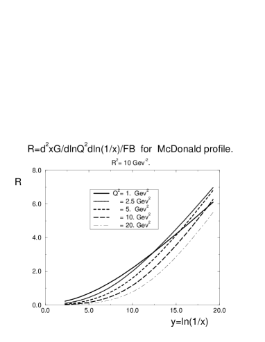
Figure 5: The comparison of $\frac{\partial^{2}xG^{GRV}(x,Q^{2})}{\partial\ln Q^{2}\,\partial\ln\frac{1}{x}}$ given by Eq. (30) with the Froissart boundary given by Eq. (32) and Eq. (33). R = $\frac{\frac{\partial^{2}xG(x,Q^{2})}{\partial\ln Q^{2}\,\partial\ln\frac{1}{x}}}{FB}$, where $FB$ is the Froissart boundary given by Eq. (32) and Eq. (33)

This boundary is much higher than the $\frac{\partial^{2}xG(x,Q^{2})}{\partial\ln Q^{2}\,\partial\ln\frac{1}{x}}$ in all current parameterizations of the gluon structure function [26] [5] [27]. However, using the approach developed in the previous section one can obtain more restrictive estimates, namely

$$\frac{\partial^{2}xG(x,Q^{2})}{\partial\ln Q^{2}\,\partial\ln\frac{1}{x}}\,\,<\,\,\frac{Q^{2}}{\pi^{2}}\,R^{2}$$ (32)

and

$$\frac{\partial^{2}xG(x,Q^{2})}{\partial\ln Q^{2}\,\partial\ln\frac{1}{x}}\,\,<\,\,\frac{2\,Q^{2}}{\pi^{2}}\,R^{2}$$ (33)

for $S(b_{\perp})$ from Eq. (21) and Eq. (22), respectively. In Fig.5 we plot $\frac{\partial^{2}xG(x,Q^{2})}{\partial\ln Q^{2}\,\partial\ln\frac{1}{x}}$ for the GRV parameterization of the gluon structure function and compare them with Eq. (32) and Eq. (33). One can see, that the gluon structure function reaches the unitarity limit ( $R$ = 1 ) at HERA kinematic region.

In Ref.[24] it has been shown that $\frac{\partial xG(x,Q^{2})}{\partial\ln\frac{1}{x}}\,\approx\,3$ from the experimental data on $F_{2}$. It means that the gluon structure function reaches the unitarity boundary at $Q^{2}_{0}\,\approx\,\frac{3\pi^{2}}{R^{2}}\,\approx\,3GeV^{2}$ ( see Eq. (32) ).

5 Parameter for the SC.

To find out the parameter for the SC let us rewrite Eq. (30) in the kinematic region where $\Omega_{GG}\,<\,1$. One obtains

$$\frac{\partial^{2}xG(x,Q^{2})}{\partial\ln Q^{2}\,\partial\ln\frac{1}{x}}\,\,=\,\,\frac{2\,Q^{2}}{\pi^{3}}\,\int d^{2}b_{\perp}\,\{\,\frac{1}{2}\,\Omega_{GG}(x,\frac{1}{Q^{2}},b_{\perp})\,\,-\,\,\frac{1}{8}\,\Omega^{2}_{GG}(x,\frac{1}{Q^{2}},b_{\perp})\}\,\,.$$ (34)

Substituting $\Omega_{GG}\,=\,\frac{N_{c}\alpha_{\rm S}\pi^{2}}{Q^{2}}\,xG(x,Q^{2})\,S(b_{\perp})$ we have

$$\frac{\partial^{2}xG(x,Q^{2})}{\partial\ln Q^{2}\,\partial\ln\frac{1}{x}}\,\,=\,\,\frac{\alpha_{\rm S}\,N_{c}}{\pi}xG(x,Q^{2})\,\,-\,\,\frac{\alpha_{\rm S}^{2}\,N_{c}^{2}\pi^{2}}{4Q^{2}}(xG(x,Q^{2}))^{2}\int db^{2}_{\perp}\,S^{2}(b_{\perp})\,\}\,\,,$$ (35)

which can be rewritten in the form

$$\frac{\partial^{2}xG(x,Q^{2})}{\partial\ln Q^{2}\,\partial\ln\frac{1}{x}}\,\,=\,\,\frac{N_{c}\,\alpha_{\rm S}}{\pi}xG(x,Q^{2})\,\cdot\,\{\,1\,\,-\,\,\frac{\kappa}{4}\,\}\,\,,$$ (36)

with

$$\kappa\,\,=\,\,\frac{\alpha_{\rm S}\,N_{c}\,\pi^{3}}{Q^{2}}xG(x,Q^{2})\int db^{2}_{\perp}\,S^{2}(b_{\perp})\,\,.$$ (37)

Figure 6: The $J/\Psi$ production without a) and with b) dissociation of the proton.

The above equation gives the same definition for $\kappa$ as Eq. (1) for exponential form of $S(b_{\perp}$) ( see Eq. (22) ). Using the new HERA data on photoproduction of J/$\Psi$ meson [6] we are able to estimate the value of $R^{2}$ in the definition of $\kappa$ , recalling that $R^{2}$ is the size of the target only in the oversimplified eikonal ( Glauber ) model. To illustrate the point we picture in Fig.6 the process of J/$\Psi$ photoproduction in the additive quark model (AQM ). We see that we have two processes with different slopes ($B$ ) in $t$ ( or in $b^{2}_{\perp}$ ): the J/$\Psi$ production without ( Fig.6a ) ($B_{el}\,=\,5\,GeV^{-2}$) and with ( Fig.6b ) ( $B_{in}\,=\,1.66\,GeV^{-2}$ ) dissociation of the proton. The AQM gives us the simplest estimates for the resulting slope ( $R^{2}$ ) in Eq. (1) if we neglect any slope from the Pomeron - J/$\Psi$ vertex in Fig.6, namely

$$\frac{1}{R^{2}}\,\,=\,\,\frac{1}{4}\,\{\,\frac{3}{2B_{el}}\,\,+\,\,\frac{1}{2B_{in}}\,\}\,\,\approx\,\,\frac{1}{5}\,GeV^{-2}\,\,.$$ (38)

This is a reason why we used $R^{2}=5\,GeV^{-2}$ in Fig.1 to estimate the scale for the SC.

In our estimates of the value of the deep inelastic structure functions at $b_{\perp}$ = 0 ( see Eq.(27) ) we used an assumption that the SC does not change the value of R. To justify this assumption we plot in Fig.7 the $x$-dependence of the average $b^{2}_{\perp}$ calculated in the Glauber (eikonal ) approach with $R^{2}=5\,GeV^{-2}$. One can see that $<b^{2}_{\perp}>$ only weakly depends on $x$ in the HERA kinematic region.

Figure 7: The $x$ - dependence of $<b^{2}_{\perp}>$ in the Glauber (eikonal) approach with $R^{2}\,=\,5GeV^{-2}$.

6 Summary.

It has been presented the derivation of the Froissart boundary for the deep inelastic structure functions.

The comparison of the Froissart boundary with HERA experimental data shows that both $F_{2}(x,Q^{2})$ and $xG(x,Q^{2})$ hit the unitarity limit at $Q^{2}\,\approx\,2-4GeV^{2}$. This fact gives rise to a challenge for theoreticians to explain the matching between the deep inelastic scattering and real photoproduction process in the framework of QCD.

We hope that this letter as well as Ref.[24] will stimulate the new round of the discussions on the theory of the shadowing corrections in the deep inelastic processes. We believe that the resolution of all difficulties could be found assuming that the SC has worked in the full in the gluon structure function and has been taken in the phenomenological initial gluon distribution in standard parameterizations [5] [26] [27]. However, much more work is needed to prove this.

This work was supported in part by the U.S. Department of Energy, Division of High Energy Physics, Contract No. W-31-109-ENG-38 and by CNPq,CAPES and FINEP,Brazil.

References

-
[1]
H1 Collaboration, T. Ahmed et al.: Nucl. Phys B439 (1995)
471;
ZEUS Collaboration, M. Derrick et al.: Z. Phys. C69 (1995) 607;
H1 Collaboration, S.Aid et al.: DESY 96-039 (1996). - [2] L. V. Gribov, E. M. Levin and M. G. Ryskin: Phys.Rep. 100 (1983) 1.
- [3] A.H. Mueller and J. Qiu: Nucl. Phys. B268 (1986) 427.
- [4] A.H. Mueller: Nucl. Phys. B335 (1990) 115; E. Levin and M. Wüsthoff: Phys. Rev. D50 (1994) 4306; J. Bartels, H. Lotter and M. Wüsthoff: Phys. Lett. B348 (1995) 589 and references therein.
- [5] M. Gluck, E. Reya and A. Vogt: Z. Phys. C53 (1992) 127.
- [6] H1 Collaboration, S.Aid et al.: DESY 96-037, March 1996.
- [7] V.N. Gribov: Sov. Phys. JETP 30 (1969) 708.
- [8] J.D. Bjorken: Proc. of the Colloqium on High Multiplicity Hadronic Interaction, Paris, May 1994, ed. A. Krzywicki (Ecole Politechique).
- [9] H. Abramowicz, L. Frankfurt and M. Strikman: DESY 95-047, March 1995.
- [10] A.H. Mueller: Nucl. Phys. B335 (1990) 115.
- [11] A.H. Mueller: Nucl. Phys. B415 (1994) 373.
- [12] E.M. Levin and M.G.Ryskin: Sov. J. Nucl. Phys. 45 (1987) 150.
- [13] E.M. Levin and M.G. Ryskin: Phys.Rep. 189 (1990) 267.
- [14] N.N. Nikolaev and B.G.Zakharov: Z. Phys. C49 (1991) 607, Z. Phys. C53 (1992) 331, Phys. Lett. B260 (1991) 414.
- [15] B.Z. Kopeliovich et al. Phys. Lett. B324 (1994) 469.
- [16] B. Blättel, L. Frankfurt and M. Strikman: Phys. Rev. Lett. 71 (1993) 896.
- [17] E. Gotsman, E. M. Levin and U. Maor: Nucl. Phys. B464 (1996) 251.
- [18] M. Froissart: Phys. Rev. 123 (1961) 1053.
- [19] A. Martin: “ Scattering Theory: Unitarity, Analyticity and Crossing”, Lecture Notes in Physics, Springer - Verlag, Berlin-Heilderberg- New York, 1969.
-
[20]
H1 Collaboration, T. Ahmed et al.: Phys. Lett. B338 (1994) 507;
ZEUS Collaboration, M. Derrick et al.: Phys. Lett. B350 (1995) 120;
H1 Collaboration, S.Aid et al.: DESY 96-037, March 1996. - [21] E. Gotsman, E. M. Levin and U. Maor: Phys. Lett. B353 (1995) 526.
-
[22]
ZEUS Collaboration, M. Derrick et al.: Phys. Lett. B345 (1995) 576;
H1 Collaboration, I.Abt et al.: Phys. Lett. B321 (1994) 161. - [23] A.D. Martin, W.J. Stirling and R.G. Roberts: Phys. Lett. B354 (1995) 155.
- [24] W. Buchmüller and D. Haidt: DESY 96-061, March 1996.
- [25] A.L. Ayala, M.B. Gay Ducati and E.M. Levin: CBPF-FN-020/96, hep-ph 9604383, April 1996.
- [26] A.D. Martin, R.G. Roberts and W.J. Stirling: Phys. Lett. B306 (1993) 145.
- [27] CTEQ Collaboration, H.L.Lai et al.: Phys. Rev. D51 (1995) 4763.