Computational Advances in the Study of Baryon Number Violation

in High Energy Electroweak Collisions

Claudio Rebbi and Robert Singleton, Jr.

Physics Department

Boston University

590 Commonwealth Avenue

Boston, MA 02215, USA

Abstract

We present some recent advances in the computational study of baryon number violation in high energy electroweak collisions. We examine classically allowed processes above the sphaleron barrier and, using a stochastic search procedure, we explore the topology changing region in the energy and particle number plane. Finding topology changing classical solutions with small incident particle number would be an indication that baryon number violation becomes unsuppressed in high energy collisions. Starting with a topology changing solution of approximately 50 incoming particles, our Monte-Carlo procedure has produced other topology changing solutions with 40% lower incident particle numbers, with energies up to one and a half times the sphaleron energy. While these solutions still involve a rather large number of incident particles, we have nonetheless demonstrated that our search procedure is effective in reducing the particle number while ensuring topology change. Taking advantage of more powerful computational resources, we plan to extend the search to still higher energies.

BUHEP-96-13

hep-ph/9606479 Typeset in LaTeX

1 Introduction

The prospect of observable high energy baryon number violation within the standard model has recently attracted widespread attention. Unfortunately, despite considerable effort by a great many theorists, the issue still remains largely unsettled. The purpose of this paper is to explain some recent computational developments that shed more light on the problem and which might help contribute to a final solution. Before we begin, however, in an effort to write a self-contained work, we shall give a brief exposition of nonperturbative baryon number violation in the standard model. We unfortunately cannot survey the vast literature on the subject with the depth it deserves, so instead a brief summary of the facts germane to our numerical approach must suffice.

For our purposes, when we talk of the “standard model” we mean the standard model in which the Weinberg angle has been set to zero, i.e. we shall be considering $SU(2)$ gauge theory spontaneously broken via a single Higgs doublet. This simplified model has all the relevant physics. Most importantly, the gauge structure dictates nontrivial topology for the bosonic vacuum sector. Working in the temporal gauge with periodic boundary conditions at spatial infinity, each vacuum may be characterized by an integer called the winding number which measures the number of times the gauge manifold is wound around 3-space[1]. As this number is a topological invariant, vacua of different winding numbers cannot be continuously deformed into one another.

Because of the axial vector anomaly, baryon number violation occurs when the gauge and Higgs fields change their topology[2]. Different topological sectors are separated by an extremely high barrier, the top of which is a static saddle-point solution to the equations of motion. This configuration is called the sphaleron[3], and it has an energy of about $10\,{\rm TeV}$ and possesses a single unstable direction in field space. At low energy the baryon number violating rates are exceedingly small, as the gauge and Higgs fields must first tunnel through the sphaleron, which is extremely unlikely indeed.

Recently the prospect of rapid baryon number violation at high temperatures and high energies has emerged. The basic idea is that if the gauge and Higgs fields have enough energy, they can change their topology by sailing over the sphaleron barrier rather than being forced to tunnel through it. At high temperatures this is precisely what happens, and it is generally agreed that baryon number violation becomes unsuppressed in the early universe[4].

The situation in high energy collisions is far less clear. The limiting process in baryon number violation is the production of a sphaleron-like configuration from an incident beam of high energy particles. But since the sphaleron is a large extended object, there is a scale mismatch with the initial high energy 2-particle state, and hence one naively expects the baryon number violating rate to be small. However, Ringwald [5] and Espinosa[6] have suggested that the sum over many-particle final states gives rise to factors that grow with energy sufficiently rapidly to offset any exponential suppression. If true, this offers the exciting prospect of one day studying baryon number violation in the laboratory. Their approach, however, neglects some important corrections which still elude calculation despite considerable effort. Apart from lattice simulations, semi-classical techniques are our only handle on nonperturbative effects. The basic problem with anomalous baryon number violation is that exclusive two-particle initial states are not very amenable to these methods, and there are potentially large initial state corrections whose effects remained undetermined.

Our efforts lie in an attempt to overcome these limitations. Many people have struggled in similar endeavors, but we only have space to summarize the work of one group upon which our approach has been partly inspired. In an effort to alleviate problems arising from exclusive two-particle states, Rubakov, Son and Tinyakov[9] consider an inclusive quantity:

$$\sigma(E,N) = \sum_{f,i}\,\mid<f|\,S\,P_{E}\,P_{N}\,|i>\mid^{2}\,$$ (1)

where the sum is over all initial and final states, $S$ is the $S$-matrix, and $P_{E}$ and $P_{N}$ are projection operators onto subspaces of energy $E$ and particle number $N$ respectively.

Unlike the exclusive two-particle cross section $\sigma_{2}(E)$, the quantity $\sigma(E,N)$ is directly calculable by semiclassical methods. If the energy and particle number are parameterized by

$$E = {\epsilon\over g^{2}}$$ (2)

$$N = {\nu\over g^{2}}\ ,$$ (3)

then in the limit $g\to 0$ with $\epsilon$ and $\nu$ held fixed, the path integral for $\sigma(E,N)$ can be saturated by a classical saddle-point solution to the equations of motion. The cross section takes the form

$$\sigma(E,N) = \exp\left[{1\over g^{2}}\,F(\epsilon,\nu)+{\cal O}(g^{0})\right]\ ,$$ (4)

where the function $F(\epsilon,\nu)$ is determined by the classical solution. These solutions naturally divide into two regimes: there is Euclidean evolution corresponding to tunneling under the sphaleron barrier, and Minkowski evolution corresponding to classical motion before and after the tunneling event.

The utility of $\sigma(E,N)$ arises because it may be used to bound $\sigma_{2}(E)$. By construction, $\sigma(E,N)$ provides an upper bound to $\sigma_{2}(E)$. A lower bound may be obtained under some reasonable physical assumptions. The two-particle process is expected to be dominated by a most favored intermediate sphaleron-like state, and the rate into this intermediate state bounds the two-particle cross section from below. Combining these upper and lower bounds allows one to write [7, 8]

$$\exp(-const\,N)\,\sigma(E,N)<\sigma_{2}(E)\,<\sigma(E,N)\ ,$$ (5)

from which it follows that[7]

$$\lim_{g\to 0}\sigma_{2}(E)=F(\epsilon,\nu)+\cal{O(\nu)}\ .$$ (6)

The consistency of the first inequality requires that $F(\epsilon,\nu)$ have a smooth $\nu\to 0$ limit, in which case $F(\epsilon,0)$ determines the exponential behavior of $\sigma_{2}(E)$. However, the second inequality of (5) holds regardless of continuity, and hence if $\sigma(E,N)$ is exponentially suppressed then so is $\sigma_{2}(E)$.

Obviously finding these Euclidean-Minkowski hybrid solutions will be extremely illuminating, and we are presently engaged in this rather formidable numerical task. In this paper, however, rather than exploring the full barrier penetration problem, we report on a complimentary approach. We examine the classically allowed regime above the sphaleron barrier in which the saddle-points that saturate the path integral are pure Minkowski solutions. This is less computationally demanding than solving the tunneling problem, while still yielding considerable information about baryon number violation. Spatial limitations prevent us from giving a full blown treatment of our numerical investigation, and the reader is referred to Ref. [10] for complete details. But the basic idea is that if a topology changing classical solution with small incident particle number could be found, this would be a strong indication that baryon number violation would be observable in high energy two-particle collisions. Conversely, if there are no small-multiplicity topology changing solutions, then it is unlikely that the rates become exponentially unsuppressed.

This can be made more precise in the following manner. Because of energy dissipation, the system will asymptotically approach vacuum values and will consequently linearize in the past and future. Field evolution then becomes a superposition of normal mode oscillators with amplitudes $a_{n}$, which allows us to define the asymptotic particle number $\nu=\sum|a_{n}|^{2}$. Furthermore, since the fields approach vacuum values in the infinite past and future, the winding numbers of the asymptotic field configurations are also well defined, and fermion number violation is given by the change in topology of these vacua[11]. Because of the sphaleron barrier, classical solutions that change topology must have energy $\epsilon$ greater than that of the sphaleron. The problem we would like to solve, then, is whether the incident particle number $\nu$ of these solutions can be made arbitrarily small. That is to say, we wish to map the region of topology changing classical solutions in the $\epsilon$-$\nu$ plane.

We could easily parameterize incoming configurations in terms of small perturbations about a given vacuum, but it would be extremely difficult to choose the parameters to ensure a subsequent change in winding number. This is because topology changing classical solutions must pass over the sphaleron barrier at some point in their evolution, which is extremely difficult arrange by an appropriate choice of initial conditions. So computationally we purse a different strategy. We shall evolve a configuration near the top of the sphaleron barrier until it linearizes and the particle number can be extracted. The time reversed solution, then, has a known incident particle number and will typically pass over the sphaleron barrier thereby changing topology. Of course we have no obvious control over the asymptotic particle number of the initial sphaleron-like configuration; however, by using suitable stochastic sampling techniques, we can systematically lower the particle number while ensuring a change of topology. This will allow us to explore the $\epsilon$-$\nu$ plane and map the region of topology change, the lower boundary of which should tell us a great deal about baryon number violation in high energy collisions.

2 Topological Transitions

Let us now put some flesh on the bones of the introductory discussion. For simplicity we consider the standard model with the Weinberg angle set to zero. The resulting spontaneously broken $SU(2)$ gauge theory possesses all the relevant physics while undergoing notable simplification. The action for the bosonic sector of this theory is

$$S=\int dx^{4}~{}\left\{-{1\over 2}{\rm Tr}\,F_{\mu\nu}F^{\mu\nu}+D_{\mu}\Phi^{\dagger}D^{\mu}\Phi-\lambda(\Phi^{\dagger}\Phi-1)^{2}\right\}\ ,$$ (7)

where the indices run from $0$ to $3$ and where

$$F_{\mu\nu} = \partial_{\mu}A_{\nu}-\partial_{\nu}A_{\mu}-i[A_{\mu},A_{\nu}]$$ (8)

$$D_{\mu}\Phi = (\partial_{\mu}-iA_{\mu})\Phi\ .$$ (9)

We use the standard metric $\eta={\rm diag}(1,-1,-1,-1)$, and have eliminated several constants by a suitable choice of units. We have also set $g=1$, but we shall restore the gauge coupling to its physical value of $g=0.652$ when needed. For our numerical work we take $\lambda=0.1$, which corresponds to a Higgs mass of about $M_{H}=72\,{\rm GeV}$.

To yield a computationally manageable system, we work in the spherical Ansatz of Ref. [12] in which the gauge and Higgs fields are parameterized in terms of six real functions $a_{0}\,,\,a_{1}\,,\,\alpha\,,\,\beta\,,\,\mu\ {\rm and}\ \nu\ {\rm of}\ r\ {\rm and}\ t$:

$$A_{0}({\bf x},t) = \frac{1}{2}\,a_{0}(r,t)\mbox{\boldmath$\sigma$}\cdot{\bf\hat{x}}$$ (10)

$$A_{i}({\bf x},t) = \frac{1}{2}\,\big{[}a_{1}(r,t)\mbox{\boldmath$\sigma$}\cdot{\bf\hat{x}}\hat{x}^{i}+\frac{\alpha(r,t)}{r}(\sigma^{i}-\mbox{\boldmath$\sigma$}\cdot{\bf\hat{x}}\hat{x}^{i})+\frac{1+\beta(r,t)}{r}\epsilon^{ijk}\hat{x}^{j}\sigma^{k}\big{]}$$ (11)

$$\Phi({\bf x},t) = [\mu(r,t)+i\nu(r,t)\mbox{\boldmath$\sigma$}\cdot{\bf\hat{x}}]\xi\ ,$$ (12)

where ${\bf\hat{x}}$ is the unit three-vector in the radial direction and $\xi$ is an arbitrary two-component complex unit vector. For the 4-dimensional fields to be regular at the origin, $a_{0}$, $\alpha$, $a_{1}-\alpha/r$, $(1+\beta)/r$ and $\nu$ must vanish like some appropriate power of $r$ as $r\to 0$.

These spherical configurations reduce the system to an effective 1+1 dimensional theory whose action can be obtained by inserting (10)-(12) into (7), from which one obtains[12]

$$S=4\pi\int dt\int^{\infty}_{0}dr \bigg{[}-\frac{1}{4}r^{2}f^{\mu\nu}f_{\mu\nu}+D^{\mu}\chi^{*}D_{\mu}\chi+r^{2}D^{\mu}\phi^{*}D_{\mu}\phi$$

$$-\frac{1}{2r^{2}}\left(~{}|\chi|^{2}-1\right)^{2}-\frac{1}{2}(|\chi|^{2}+1)|\phi|^{2}-{\rm Re}(i\chi^{*}\phi^{2})$$

$$-\lambda\,r^{2}\,\left(|\phi|^{2}-1\right)^{2}~{}\bigg{]}\ ,$$

where the indices now run from $0$ to $1$ and are raised and lowered with $\eta_{\mu\nu}={\rm diag}(1,-1)$, and where

$$f_{\mu\nu} = \partial_{\mu}a_{\nu}-\partial_{\nu}a_{\mu}\$$ (14)

$$\chi = \alpha+i\beta$$ (15)

$$\phi = \mu+i\nu\$$ (16)

$$D_{\mu}\chi = (\partial_{\mu}-i\,a_{\mu})\chi$$ (17)

$$D_{\mu}\phi = (\partial_{\mu}-\frac{i}{2}\,a_{\mu})\phi\ .$$ (18)

This is an effective 2-dimensional $U(1)$ gauge theory spontaneously broken by two scalar fields. It possesses the same rich topological structure as the full 4-dimensional theory and provides an excellent testing ground for numerical exploration.

Vacuum states of the effective 2-dimensional theory are characterized by $|\chi|=|\phi|=1$ and $i\chi^{*}\,\phi=-1$ (as well as $D_{\mu}\chi=D_{\mu}\phi=0)$. The vacua then take the form

$$a_{\mu\,\rm vac} = \partial_{\mu}\Omega$$ (19)

$$\chi_{\rm vac}\, = -i\,e^{i\Omega}$$ (20)

$$\phi_{\rm vac}\, = \pm\,e^{i\Omega/2}\ ,$$ (21)

where the gauge function $\Omega=\Omega(r,t)$ is required to vanish at $r=0$ to ensure regularity of the 4-dimensional fields. Furthermore, like the full 4-dimensional theory, these vacua still possesses nontrivial topological structure. Compactification of 3-space requires that $\Omega(r,t)\to 2\pi n$ as $r\to\infty$, in which case the winding number of such vacua in the the $a_{0}=0$ gauge is simply the integer $n$. Note that as $r$ varies from zero to infinity, $\chi$ winds $n$ times around the unit circle while $\phi$ only winds by half that amount.

Since the winding number is a topological invariant, a continuous path connecting two inequivalent vacua must at some point leave the manifold of vacuum configurations. Along this path there will be a configuration of maximal energy, and of all such maximal energy configurations there exists a unique one of minimal energy[3]. This configuration is called the sphaleron and may conveniently be parameterized by

$$a^{\mu}_{\rm sph}(r) = 0\ ,$$

$$\chi_{\rm sph}(r) = i[2f(r)-1]$$ (22)

$$\phi_{\rm sph}(r) = ih(r)$$

where the profile functions $f$ and $h$ vanish at $r=0$, tend to unity as $r\to\infty$ and are otherwise determined by minimizing the energy functional. The energy of the sphaleron depends very weakly on the Higgs mass and is about $M_{w}/g^{2}\sim 10~{}{\rm TeV}$, or $\epsilon=4\pi\,(2.54)$ in the units we are using.

Figure 1: The $\chi$ and $\phi$ fields for a vacuum-to-vacuum topology changing transition in a gauge inconsistent with compactified 3-space. The scalar fields are traced in the complex plane as the the spatial coordinate spans the entire axis. Figs. (a) and (c) represent two inequivalent topological vacua while (b) is the sphaleron barrier separating them.

While this form of the sphaleron in which $a_{\mu}$ vanishes and $\chi$ and $\phi$ are pure imaginary is convenient for numerical work, it does have a slight peculiarity that we briefly mention. Recall that compactification of 3-space requires the gauge function $U$ to approach an even multiple of $2\pi$ as $r\to\infty$. It is possible to relax this restriction, and it will often be convenient to choose a gauge in which $U\to(2n+1)\pi$ as $r\to\infty$, in which case $\chi_{\rm vac}\to i$ and $\phi_{\rm vac}\to\pm i$. This is precisely the large-$r$ boundary condition of the sphaleron, which illustrates that (2) is inconsistent with spatial compactification. There is of course nothing wrong with this, and a topological transition of unit winding number change in this gauge is illustrated in Fig. 1. Rather than $\chi$ winding once around the unit circle, it instead winds over the left hemisphere before the transition and over the right after the transition. The total phase change is still $2\pi$, as it must be since this is a gauge invariant quantity.

Throughout most of this paper we shall use a gauge consistent with (2) in which space cannot be compactified. From a computational perspective, this will make perturbations about the sphaleron more easily parameterized. There will, however, be times in which it is more convenient to impose spatial compactification, but we will always alert the reader to such a change of gauge.

3 Classical Evolution

So far we have primarily been considering topology changing sequences of configurations, not necessarily solutions of the equations of motion. Now we turn to the classical evolution of the system. We will consider solutions that linearize in the distant past and future, and hence ones that asymptote to specific topological vacua. This allows us to define the incident particle number, and it makes clear what is meant by topology change of a classical solution (namely, the change in winding number of the asymptotic vacua).

The field equations are coupled nonlinear particle differential equations, and must be solved computationally on the lattice. But before we present our numerical procedure, we first formulate the problem in the continuum. The equations of motion resulting from the action (2) are

$$\partial^{\mu}(r^{2}f_{\mu\nu})=i\left[D_{\nu}\chi^{*}\chi-\chi^{*}D_{\nu}\chi\right]+\frac{i}{2}\,\,r^{2}\left[D_{\nu}\phi^{*}\phi-\phi^{*}D_{\nu}\phi\right]$$ (23)

$$\left[D^{2}+\frac{1}{r^{2}}(|\chi|^{2}-1)+\frac{1}{2}\,|\phi|^{2}~{}\right]\chi=-\frac{i}{2}\,\,\phi^{2}$$ (24)

$$\left[D^{\mu}r^{2}D_{\mu}+\frac{1}{2}(|\chi|^{2}+1)+2\lambda r^{2}\left(|\phi|^{2}-1\right)\right]\phi=i\,\chi\phi^{*}\ .$$ (25)

The $\nu=0$ equation in (23) is not dynamical but is simply the Gauss’s law constraint.

To solve these equations, we must supplement them with boundary conditions. The conditions at $r=0$ can be derived by requiring the 4-dimensional fields to be regular at the origin. The behavior as $r\to 0$ must be

$$a_{0} = a_{0,1}r+a_{0,3}r^{3}+\dots$$ (26)

$$a_{1} = a_{1,0}+a_{1,2}r^{2}+\dots$$ (27)

$$\alpha = \alpha_{1}r+\alpha_{3}r^{3}+\dots$$ (28)

$$\beta = -1+\beta_{2}r^{2}+\dots$$ (29)

$$\mu = \mu_{0}+\mu_{2}r^{2}+\dots$$ (30)

$$\nu = \nu_{1}r+\nu_{3}r^{3}+\dots\ ,$$ (31)

where the coefficients of the $r$-expansion are undetermined functions of time. The $r$-behavior of the various terms are determined by the requirement that it has the appropriate power of $r=(x^{2}+y^{2}+z^{2})^{1/2}$ to render the 4-dimensional fields analytic in terms of $x$, $y$ and $z$. For example, $a_{0}$ must be odd in $r$ since $A_{0}$ is proportional to $a_{0}\mbox{\boldmath$\sigma$}\cdot{\bf\hat{x}}=(a_{0}/r)\mbox{\boldmath$\sigma$}\cdot{\bf x}$. In terms of $\chi$ and $\phi$ the boundary conditions at $r=0$ become

$$a_{0}(0,t) = 0$$ (32)

$$\chi(0,t) = -i$$ (33)

$${\rm Re}\,\partial_{r}\phi(0,t) = 0$$ (34)

$${\rm Im}\,\phi(0,t) = 0\ .$$ (35)

There is another $r=0$ boundary condition which arises from the requirement that $a_{1}-\alpha/r$ be regular as $r\to 0$. This condition can be written as $a_{1,0}=\alpha_{1}$, and once imposed on initial configurations it remains satisfied at subsequent times because of Gauss’s law.

We turn now to the large-$r$ boundary conditions. Finite energy configurations must approach pure vacuum at spatial infinity, and we may choose a gauge in which

$$a_{\mu}(r,t) \to 0$$ (36)

$$\chi(r,t) \to i$$ (37)

$$\phi(r,t) \to i$$ (38)

as $r\to\infty$. This choice of gauge does not admit spatial compactification, but nonetheless it is numerically conveniently since it is consistent with the simple parameterization of the sphaleron (2). At times we will choose a gauge consistent with spatial compactification in which $\chi(r,t)\to-i$ and $\phi(r,t)\to 1$ as $r\to\infty$, but unless otherwise specified we will take the large-$r$ boundary conditions to be (36)-(38).

The field equations (23)-(25), together with boundary conditions (32)-(38), may now be used to evolve initial profiles and investigate their subsequent topology change. The evolution is performed by discretizing the system using the methods of lattice gauge theory, in which we subdivide the $r$-axis into $N$ equal intervals of length $\Delta r$ with finite extent $L=N\Delta r$ (in our numerical simulations we take $N=2239$ and $\Delta r=0.04$). The field theoretic system then becomes finite and may be solved using standard numerical techniques.

The fields $\chi(r,t)$ and $\phi(r,t)$ become discrete variables $\chi_{i}(t)$ and $\phi_{i}(t)$ associated with the lattice sites $r_{i}=i\Delta r$ where $i=0\cdots N$. The continuum boundary conditions render the variables at the spatial end-points nondynamical, taking the values $\chi_{0}=-i$, $\chi_{N}=i$ and $\phi_{N}=i$ (the value of $\phi_{0}$ will be discussed momentarily). The time component of the gauge field $a_{0}(r,t)$ is also associated with the lattice sites and is represented by the variables $a_{0,i}(t)$ with $i=0\cdots N$. We will usually work in the temporal gauge in which $a_{0,i}=0$, and we will not concern ourselves with this degree of freedom.

The spatial components of the gauge field $a_{1}(r,t)$ become discrete variables associated with the oriented links of the lattice, and we represent them by $a_{1,i}(t)\equiv a_{i}(t)$ located at positions $r_{i+1/2}=(i+1/2)\Delta r$ with $i=0\cdots N-1$. The covariant spatial derivatives become covariant finite difference operators that are also associated with the links, e.g.

$$D_{r}\phi\to{\exp[-ia_{i}\,\Delta r/2]\,\phi_{i+1}-\phi_{i}\over\ \Delta r}{}~{}~{}~{}~{}~{}~{}~{}i=0\cdots N-1\ .$$ (39)

where $a_{i}$ is short-hand notation for $a_{1,i}$.

It is now straightforward to discretize the action (2) in a manner that still possesses an exact local gauge invariance. But first, we need to state the restriction on $\phi_{0}(t)$ corresponding to the boundary conditions (34) and (35). Since $a_{1}$ is real, we can write these boundary conditions in a covariant fashion by requiring the real part of $D_{r}\phi$ and the imaginary part of $\phi$ to vanish at $r=0$. Using the discretized operator (39), we can then solve this boundary condition for $\phi_{0}$ to obtain

$$\phi_{0}={\rm Re}[\exp(-i\,a_{0}\,\Delta r/2)\phi_{1}]\ ,$$ (40)

where $a_{0}$ is the value of $a_{1,i}$ at $i=0$ and should not be confused with the time-like vector field. This now allows us to eliminate $\phi_{0}$ from the list of dynamical variables.

Finally, the discretized Lagrangian becomes

$$L = 4\pi\,\sum_{i=0}^{N-1}\bigg{\{}\frac{r^{2}_{i+1/2}}{2}\,\bigg{(}\partial_{0}a_{i}-\frac{a_{0,i+1}-a_{0,i}}{\Delta r}\bigg{)}^{2}-\frac{|\exp(-i\,a_{i}\,\Delta r)\chi_{i+1}-\chi_{i}|^{2}}{\Delta r^{2}}\bigg{\}}\Delta r$$

$$\hskip-36.135pt+\,4\pi\,\sum_{i=1}^{N-1}\bigg{\{}|(\partial_{0}-ia_{0,i})\chi_{i}|^{2}+r^{2}_{i}\,|(\partial_{0}-{ia_{0,i}\over 2})\phi_{i}|^{2}-r^{2}_{i+1/2}\,\frac{|\exp({-i\,a_{i}\,\Delta r/2})\phi_{i+1}-\phi_{i}|^{2}}{\Delta r^{2}}$$

$$\hskip-36.135pt-\frac{1}{2}\,(|\chi_{i}|^{2}+1)|\phi_{i}|^{2}-{\rm Re}(i\chi_{i}^{*}\phi_{i}^{2})-{1\over 2r^{2}_{i}}(|\chi_{i}|^{2}-1)^{2}-\lambda r^{2}_{i}\,(|\phi_{i}|^{2}-1)^{2}\bigg{\}}\Delta r$$

$$\hskip-36.135pt-\,4\pi\,r^{2}_{1/2}{[{\rm Im}(\exp(-i\,a_{0}\,\Delta r/2)\phi_{1})]^{2}\over\Delta r}\ ,$$

and the system may now be evolved using standard numerical techniques of ordinary differential equations. The Lagrangian (3) is actually of a Hamiltonian type with no dissipative terms, so it is convenient to use the leapfrog algorithm to perform the numerical integration.

We do not have space to outline this well known computational procedure, so instead we simply state some of its more attractive features. First, the algorithm is second order accurate (i.e. the error from time discretization is of order $(\Delta t)^{3}$ in the individual steps and of order $(\Delta t)^{2}$ in an evolution of fixed length). Second, energy is exactly conserved in the linear regime, a desirable feature when pulling out the particle number. And finally, the algorithm possesses an exact discretized-time invariance, which is important since we are interested in obtaining the time reversed solutions starting from perturbations about the sphaleron. Of course these last two properties hold exactly only up to round-off errors, which can be made quite small by using double precision arithmetic.

4 The Initial Configuration: Perturbation About the Sphaleron

We are now ready to continue our investigation into the connection between the incident particle number of a classical solution and subsequent topology change. We could proceed by parameterizing linear incoming configurations of known particle number, but it would be extremely difficult to arrange the classical trajectory to traverse the sphaleron barrier. If we failed to see topology change for a given initial configuration, we could never be sure whether it was simply forbidden in principle by the choice of incident particle number, or simply because the initial trajectory was pointed the wrong direction in field space.

To alleviate this difficulty, we have chosen to evolve initial configurations at or near the moment of topology change, and when the linear regime is reached the particle number will be extracted in the manner explained shortly. The physical process of interest is then the time reversed solution that starts in the linear regime with known particle number and subsequently proceeds over the sphaleron barrier. Of course we must explicitly check whether topology change in fact occurs, but we have found that it usually does. Fig. 2 illustrates the numerical evolution of the $\chi$ field for a typical topology changing solution obtained in this manner. The modulus of $\chi$ is represented by the height of the surface, while the phase is color coded (but unfortunately we can only reproduce the figure in gray scale). We have reverted to a gauge in which $\chi_{N}=-i$ and $\phi_{N}=1$, consistent with spatial compactification, and in which the incoming state has no winding and the outgoing state has unit winding number. The topology change is represented by the persistent strip of $2\pi$ phase change near the origin after the transition.

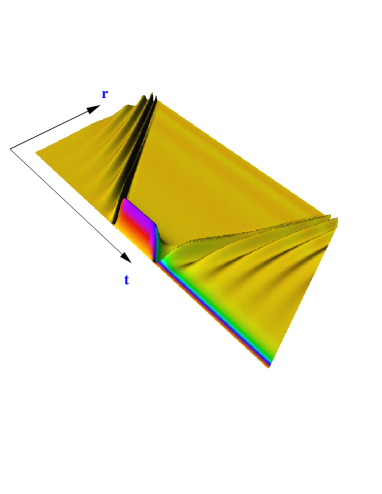
Figure 2: Topology changing transition: behavior of the $\chi$ field obtained the time reversal procedure described in the text. The various shades of gray code the phase of the complex field. The field starts as an excitation about the trivial vacuum, passes over the sphaleron and then emerges as an excitation about the vacuum of unit winding. Note the persistent strip of $2\pi$ phase change near $r=0$ after the wave bounces off the origin.

We turn now to parameterizing initial configurations. For classical solutions that dissipate in the past and future, topology change (and hence baryon number violation) is characterized by zeros of the Higgs field[11]. For such topology changing solutions in the spherical Ansatz, the $\chi$ field, which parameterizes the transverse gauge degrees of freedom, must also vanish at some point in its evolution. However, unless the transition proceeds directly through the sphaleron, the zeros of $\phi$ and $\chi$ need not occur simultaneously, and for convenience we shall choose to parameterize the initial configuration at the time in which $\chi$ vanishes for some nonzero $r$. Furthermore, we can exhaust the remaining gauge freedom by taking the initial $\chi$ to be pure imaginary. We thus parameterize the initial conditions as an expansion in terms of some appropriate complete set with coefficients $c_{n}$, consistent only with the boundary conditions and the requirement that $\chi$ be pure imaginary with a zero at some $r>0$.

We choose to parameterize initial conditions in terms of perturbations about the sphaleron given by linear combinations of spherical Bessel functions consistent with the small-$r$ behavior (26)-(31). We only need the first three functions

$$j_{0}(x) = \frac{\sin x}{x}$$ (42)

$$j_{1}(x) = \frac{\sin x}{x^{2}}-\frac{\cos x}{x}$$ (43)

$$j_{2}(x) = \left(\frac{3}{x^{3}}-\frac{1}{x}\right)\sin x-\frac{3}{x^{2}}\cos x\ ,$$ (44)

since $j_{0}(x)\sim 1$, $j_{1}(x)\sim x$ and $j_{2}(x)\sim x^{2}$ at small $x$. We also require the perturbations to vanish at $r=L$ consistent with the large-$r$ boundary conditions (36)-(38). We then parameterize perturbations about the sphaleron in terms of $j_{nm}(r)=j_{n}(\alpha_{nm}r)$ with $n=0,1,2$, where $\alpha_{nm}$ with $m=1,2,\cdots\,$ are the zeros of $j_{n}(x)$. We are thus led to parameterize the initial conditions as

$$\chi(r,0) = \chi_{\rm sph}(r)+i\sum_{m=1}^{N_{\rm sph}}\,c_{1m}\ j_{2m}(r)$$ (45)

$$\phi(r,0) = \phi_{\rm sph}(r)+\sum_{m=1}^{N_{\rm sph}}\,c_{2m}\ j_{0m}(r)+i\sum_{m=1}^{N_{\rm sph}}\,c_{3m}\ j_{1m}(r)$$ (46)

$$\dot{\chi}(r,0) = \sum_{m=1}^{N_{\rm sph}}\,c_{4m}\ j_{1m}(r)+i\sum_{m=1}^{N_{\rm sph}}\,c_{5m}\ j_{2m}(r)$$ (47)

$$\dot{\phi}(r,0) = \sum_{m=1}^{N_{\rm sph}}\,c_{6m}\ j_{0m}(r)+i\sum_{m=1}^{N_{\rm sph}}\,c_{7m}\ j_{1m}(r)$$ (48)

$$a_{1}(r,0) = \sum_{m=1}^{N_{\rm sph}}\,c_{8m}\ j_{2m}(r)\ ,$$ (49)

where $\chi_{\rm sph}$ and $\phi_{\rm sph}$ are the sphaleron profiles, and where the sum is cut off at $N_{\rm sph}\leq N$. To avoid exciting short wave length modes corresponding to lattice artifacts, we shall take $N_{\rm sph}\sim N/50$ (in our numerical work, $N_{\rm sph}=50$ for $N=2239$).

We have used continuum notation, but (45)-(48) is to be thought of as defining $\chi$ and $\phi$ on the lattice sites $r_{i}$ and $a_{1}$ on the links $r_{i+1/2}$. The time derivative of $a_{1}$ is to be determined by Gauss’s law.

5 Normal Modes and Particle Number

We are now in a position to discuss the manner in which the asymptotic particle number is to be extracted. Recall that once the system has reached the linear regime it can be represented as a superposition of normal modes, and the particle number can be defined as the sum of the squares of the normal mode amplitudes. Since we have put the system on a lattice, we should properly calculate these amplitudes using the exact normal modes of the discrete system. However, since our lattice is very dense ($N=2239$ with $\Delta r=0.04$), it suffices to project onto the normal modes of the corresponding continuum system of finite extent $L=N\Delta r$, the advantage being that we can solve for the continuum normal modes analytically. We have checked that this procedure agrees extremely well with projecting onto normal modes of the discrete system (obtained numerically), so for clarity we present only the continuum modes.

It is convenient to work in terms of the gauge invariant variables of Ref. [13]. We write the fields $\chi$ and $\phi$ in polar form,

$$\chi = -i\left[1+y\right]\,e^{i\theta}$$ (50)

$$\phi = \left[1+{h\over r}\,\right]\,e^{i\eta}\ ,$$ (51)

where the variables $y$ and $h$ are gauge invariant. We can also define the gauge invariant angle

$$\xi=\theta-2\eta\ .$$ (52)

Finally, in 1+1 dimensions we can write

$$r^{2}f_{\mu\nu}=-2\epsilon_{\mu\nu}\psi$$ (53)

where $\epsilon_{01}=+1$ and $\mu$, $\nu$ run over $0$ and $1$, and where the variable $\psi$ is gauge invariant. Rather than working with the six gauge-variant degrees of freedom $\chi$, $\phi$ and $a_{\mu}$ we use the four gauge invariant variables $\rho$, $\sigma$, $\psi$ and $\xi$.

We wish to find the equations of motion for small linearized fluctuations about the vacuum. In gauge invariant coordinates the vacuum takes the form $h_{\rm vac}=y_{\rm vac}=\psi_{\rm vac}=\xi_{\rm vac}=0$, and we thus need only work to linear order in the variables. From Ref. [13] the normal mode equations are

$$\Biggl{(}\partial_{\mu}\partial^{\mu}+4\lambda\Biggr{)}\,h = 0$$ (54)

$$\Biggl{(}\partial_{\mu}\partial^{\mu}+\frac{1}{2}+\frac{2}{r^{2}}\Biggr{)}\,y = 0$$ (55)

$$\partial^{\mu}\left\{\frac{\partial_{\mu}\psi-\epsilon_{\mu\nu}\partial^{\nu}\xi}{1+\frac{1}{4}r^{2}}\right\}+\frac{2}{r^{2}}\,\psi = 0$$ (56)

$$\partial^{\mu}\left\{\frac{\frac{1}{4}r^{2}\partial_{\mu}\xi+\epsilon_{\mu\nu}\partial^{\nu}\psi}{1+\frac{1}{4}r^{2}}\right\}+\frac{1}{2}\xi = 0\ .$$ (57)

Equation (54) corresponds to a pure Higgs excitation characterized by mass $M_{H}=2\sqrt{\lambda}$, while (55)-(57) correspond to three gauge modes of mass $M_{W}=1/\sqrt{2}$.

Note that there are four types of normal modes. The first two are easily obtained by solving the independent equations (54) and (55), while the last two can be found by solving the coupled equations (56) and (57) involving $\psi$ and $\xi$. A solution in the linear regime can then be expanded as a combination of these four modes and the amplitudes $a_{kn}$, with $k=1,2,3,4$ specifying the mode type, extracted. The Higgs and gauge particle numbers are defined by

$$\nu_{\rm higgs} = \sum_{n=1}^{N_{\rm mode}}|a_{1n}|^{2}$$ (58)

$$\nu_{\rm gauge} = \sum_{n=1}^{N_{\rm mode}}\left\{|a_{2n}|^{2}+|a_{3n}|^{2}+|a_{4n}|^{2}\right\}\ ,$$ (59)

with total particle number given by

$$\nu=\nu_{\rm higgs}+\nu_{\rm gauge}\ .$$ (60)

To avoid counting lattice artifacts we take the ultraviolet cutoff on the mode sums to be given by $N_{\rm mode}\sim N/5$ to $N/10$.

Space does not permit a detailed exposition of this procedure, and one should consult Ref. [10] for full details. Here we must be content with Fig. 3, which displays the behavior of the particle number in the four modes of oscillation as a function of time. The initial state was a typical perturbation about the sphaleron as described in the previous section, and as it evolves it quickly linearizes and settles down into a definite asymptotic particle number.

Figure 3: Decay of a small perturbation about the sphaleron: behavior of the particle number in the four modes as function of time for lattice parameters $N=2239$, $\Delta r=0.04$ and $N_{\rm mode}=200$ with $\lambda=0.1$. The physical particle numbers are obtained by multiplying the asymptotic values in the graph by $4\pi/g^{2}\sim 30$, which gives $N_{\rm higgs}\sim 8$ and $N_{\rm gauge}\sim 45$, for a total physical particle number of $N_{\rm phys}\sim 53$.

6 Stochastic Sampling of Initial Configurations

Recall that our computational strategy consists in evolving a configuration near the top of the sphaleron barrier until it linearizes, at which point the particle number can be extracted and the time reversed solution used to generate the topology changing process of interest. We can regard the energy $\epsilon$ and the asymptotic particle number $\nu$ as functions of the parameters $c_{n}$ that specify the initial configuration, and by varying these coefficients we would like to explore the $\epsilon$-$\nu$ plane and attempt to map the region of topology change. In particular, for a given energy $\epsilon$, we would like to find the minimum allowed particle number $\nu_{\rm min}(\epsilon)$ consistent with a change of topology. If this number can be made arbitrarily small, this would be a strong indication that baryon number violation would be observable in a two-particle collision.

By randomly exploring the initial configuration space parameterized by the coefficients $c_{n}$, we would stand little chance of making headway. Instead, we shall employ stochastic sampling techniques, which are ideal for tackling this type of multi-dimensional minimization. Our procedure will be to generate initial configurations weighted by $W=\exp(-F)$ with $F=\beta\,\epsilon+\mu\,\nu$, and by adjusting the parameters $\beta$ and $\mu$ we can explore selected regions in the $\epsilon$-$\nu$ plane. In particular, by increasing $\mu$ we can drive the system to lower and lower values of $\nu$ for a given $\epsilon$. In our numerical work we typically take $\beta$ between 50 and 1000 while $\nu$ ranges between 1000 to 20000.

To generate the desired distributions we have used a Metropolis Monte-Carlo algorithm. Starting from a definite configuration parameterized by $c_{n}$, we perform an upgrade to $c_{n}\to c^{\prime}_{n}=c_{n}+\Delta c_{n}$ where $\Delta c_{n}$ is Gaussian distributed with a mean of about 0.0008. We evolve the updated configuration until it linearizes and then calculate $\Delta F=\beta\,\Delta\epsilon+\mu\,\Delta\nu$. If the topology of the physically relevant time reversed solution does not change, then we discard the updated configuration. Otherwise we accept it with conditional probability $p={\rm Min}[1,\exp(-\Delta F)]$, which is equivalent to always accepting configurations that decrease $F$ while accepting those that increase $F$ with conditional probability $\exp(-\Delta F)$.

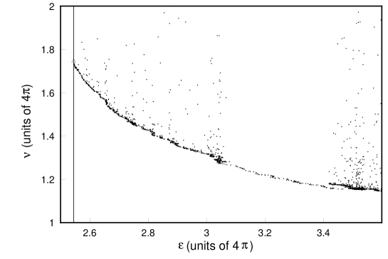
Figure 4: Monte Carlo results with lattice parameters of $N=2239$, $\Delta r=0.04$ (giving L=89.56), $N_{\rm mode}=200$ and $N_{\rm sph}=50$, and with a Higgs self-coupling of $\lambda=0.1$. The solid line marks the sphaleron energy $\epsilon_{\rm sph}=4\pi(2.5426)$, below which no topology changing process can lie. The triangle represents the configuration from which we seeded our Monte Carlo search. To obtain quantities in physical units, multiply the numbers along the axes by $4\pi/g^{2}\sim 30$. The energy axis extends from about $10{~{}\rm TeV}$ to $15{~{}\rm TeV}$, while the particle number axis ranges from about $30$ particles to $60$.

We are now in a position to present our numerical results. Fig. 4 represents 300 CPU hours and involves 30000 solutions (of which only 3000 are shown) obtained on the CM-5, a 64 node parallel supercomputer. We have chosen the lattice parameters $N=2239$, $\Delta r=0.04$, with ultraviolet cutoffs determined by $N_{\rm sph}=50$ and $N_{\rm mode}=200$. The Higgs self-coupling was taken to be $\lambda=0.1$, which corresponds to a Higgs mass of $M_{H}=72\,{\rm GeV}$.

We have managed to produce a marked decrease of about 40% in the minimum particle number $\nu_{\rm min}(\epsilon)$, which is approximated by the lower boundary in the Fig. 4. Nowhere, however, in the explored energy range does $\nu$ drop below $4\pi$, or in physical units the incident particle number $N\geq 30$ for energy $E\leq 15\,{\rm TeV}$ (the outgoing particle number tends to be about 50 to 100). This is a far cry from two incoming particles which would be necessary to argue that baryon number becomes unsuppressed in high energy collisions.

The complex nature of the solution space can be illustrated by the break in population density between $\epsilon/4\pi\sim 3$ and $\epsilon/4\pi\sim 3.4$. In our first extended search we did not check whether topology change actually occurred, trusting that the time reversed solutions would continue over the sphaleron barrier. However, we later found an entire region between $\epsilon/4\pi\sim 3$ and $\epsilon/4\pi\sim 3.4$ in which the solutions never left the original topological sector. We excluded these points and restarted our search procedure near $\epsilon/4\pi\sim 3$. A small discontinuity in the lower boundary with slightly lower particle number was produced, but we have still managed to approximate $\nu_{\rm min}(\epsilon)$ remarkably well.

We can extract more information from the system by investigating the asymptotic spectral distribution $|a_{kn}|^{2}$ as a function of mode number $n$. Before we started the search, our seed configuration (represented by the triangle in Fig. 4) linearized into a distribution that was heavily peaked about a small mode number $n_{\rm pk}\sim 50$ (with $\Delta n\sim 50$), corresponding to a frequency of $\omega_{\rm pk}\sim\pi n_{\rm pk}/L\sim 0.1$. After the search the solutions underwent a dramatic mode redistribution. The amplitudes $|a_{kn}|^{2}$ of the linear regime peaked at higher mode number, $n_{\rm pk}\sim 75-100$, with a much broader distribution ($\Delta n\sim 200$). Clearly our search procedure is very efficient in redistributing the mode population density.

While $\nu$ remains large throughout the energy range we have explored, it is interesting to note that $\nu_{\rm min}(\epsilon)$ maintains a slow but steady decrease with no sign of leveling off. To obtain an indication of the possible behavior of $\nu_{\rm min}(\epsilon)$ at higher energies, we performed fits to our data using functional forms which incorporate expected analytical properties of the boundary of the domain of topology changing solutions. The fits gave a particle number $N=2$ at energies in the range of $100\,{\rm TeV}$ to $450\,{\rm TeV}$. Of course we must explore higher energies before drawing define conclusions, but this is at least suggestive that particle number might at some point become small.

While the energy range we have explored is of limited extent and more numerical work is clearly called for, it is still remarkable that we have extracted such a wealth of information from such an analytically intractable field theoretic system. Computational techniques offer considerable promise in probing the nonlinear dynamics of the standard model, and we fully expect them to play a prominent role in our future understanding of high energy baryon number violation, both in extending the energy range of the classically allowed processes and obtaining information on the classically forbidden processes below the barrier.

Acknowledgments

This research was supported in part under DOE grant DE-FG02-91ER40676 and NSF grant ASC-940031. We wish to thank V. Rubakov for very interesting conversations which stimulated the investigation described here, A. Cohen, K. Rajagopal and P. Tinyakov for valuable discussions, and T. Vaughan for participating in an early stage of this work.

References

- [1] R. Jackiw and C. Rebbi, Phys. Rev. Lett. 37 (1976) 172; C. Callan Jr., R. Dashen and D. Gross, Phys. Lett. 63B(1976) 334.
- [2] G. ’t Hooft, Phys. Rev. D14 (1976) 3432.
-
[3]
N. Manton, Phys. Rev. D28 (1983) 2019;
F. Klinkhamer and N. Manton, Phys. Rev. D30 (1984) 2212. - [4] V. Kuzmin, V. Rubakov and M. Shaposhnikov, Phys. Lett. B155 (1985) 36.
- [5] A. Ringwald, Nucl. Phys. B330 (1990) 1.
- [6] O. Espinosa, Nucl. Phys. B343 (1990) 310.
- [7] P. Tinyakov, Phys. Lett. B 284, 410 (1992).
- [8] H. Aoyama and H. Goldberg, Phys. Lett. B 188, 506 (1987); H. Goldberg, Phys. Lett. B 257, 346 (1991); S. Khlebnikov, A. Rubakov and P. Tinyakov, Nucl. Phys. B367, 310 (1991).
- [9] V. Rubakov, D. Son and P. Tinyakov, Phys. Lett. B287 (1992) 342.
- [10] C. Rebbi and R. Singleton, Jr., “Computational Study of Baryon Number Violation in High Energy Electroweak Collisions“, hep-ph/9601260, BUHEP-95-33, to be published in Phys. Rev. D53, (1996).
- [11] E. Farhi, J. Goldstone, S. Gutmann, K. Rajagopal and R. Singleton Jr., Phys. Rev. D51 (1995) 4561, hep-ph/9410365.
- [12] B. Ratra and L. Yaffe, Phys. Lett. B205 (1988) 57.
- [13] E. Farhi, K. Rajagopal and R. Singleton Jr., Phys. Rev. D52 (1995) 2394, hep-ph/9503268.