Measuring SUSY Parameters at LEP II
Using Chargino Production and Decay

Abstract

Previously, in the context of the minimal supersymmetric standard model (without a priori assumptions of parameter unification), we studied the constraints on weak-scale SUSY parameters from chargino production at LEP II, using as observables $m_{\tilde{\chi}^{\pm}_{1}}$, $m_{\tilde{\chi}^{0}_{1}}$, the cross section and the leptonic branching fraction. Here, exploiting the high degree of polarization in chargino production, we add to our earlier work the forward-backward asymmetries of the visible hadrons and leptons in chargino decays. For a chargino that is mostly gaugino, the parameter space can now be restricted to a small region; $\tan\beta$ is constrained, the soft electroweak gaugino and electron sneutrino masses are determined to about 10%, and the sign of $\mu$ may be determined. Constraints for a chargino that is mostly Higgsino are much weaker, but still disfavor the hypothesis that the chargino is mostly gaugino. For a chargino which is a roughly equal mixture of Higgsino and gaugino, we find intermediate results.

I Introduction

One of the main goals of the LEP II $e^{+}e^{-}$ collider at CERN [1] will be to search for signs of weak-scale supersymmetry (SUSY) [2]. If particles are discovered whose quantum numbers suggest they might be SUSY partners of known particles, the immediate issues will be to determine whether these particles really behave in accordance with SUSY, and, if so, what values are assumed at the electroweak scale by the parameters of the SUSY Lagrangian. Among the many new particles that might be found, the chargino, a mixture of the $W$-fermion (Wino) and charged Higgs-fermions (Higgsinos), is of particular interest. From the theoretical standpoint, charginos are expected to be lighter than gluinos, and in many models they are lighter than most or all squarks and sleptons[3]. If kinematically accessible, charginos have a large cross section throughout SUSY parameter space, produce a clean signal in certain decay modes, and have properties that depend on a number of interesting SUSY parameters. As the chargino pair production cross section rises rapidly above threshold, each step in collider energy holds the promise not only of chargino discovery, but also of detailed SUSY studies from chargino events.

Our goal in this paper, following on our earlier work [4], is to gain insight into the properties of charginos and to estimate the ability of LEP II to determine the parameters of SUSY using charginos. This issue was also addressed by Leike in Ref. [5], where certain SUSY parameters were assumed to take specific values, and in the work of Diaz and King[6] in the context of the five-parameter minimal supergravity scenario. Our approach here is to avoid theoretical assumptions about physics at high energy scales (such as the SUSY-breaking, GUT, or Planck scale), and instead to exploit the fact that any given SUSY process is often strongly sensitive to only a small subset of the SUSY parameters in the electroweak-scale effective Lagrangian. For chargino events, we find that, after applying testable, phenomenologically-motivated assumptions, only six parameters enter strongly. Although the resulting parameter space is still rather complicated, we have developed effective methods in Ref. [4] for understanding our results and for displaying the qualitative relationship between observables and the underlying SUSY parameters. If charginos are discovered, these methods may also prove very useful for interpreting the correlated constraints on the parameter space that will come from detailed global fits.

In our previous paper we considered the case where charginos decay through virtual $W$-bosons, squarks and sleptons to the lightest neutralino (which we assumed was stable or metastable) and two leptons or light quarks. Given this phenomenology, we investigated observables that are independent of all angular distributions and thus can be studied analytically at arbitrary beam energy. These four observables are the chargino mass $m_{\tilde{\chi}^{\pm}_{1}}$, the neutralino mass $m_{\tilde{\chi}^{0}_{1}}$, the total cross section $\sigma_{\rm total}$ and the branching fraction $B_{l}$ of chargino decays to leptons. We showed that strong constraints on the weak-scale parameters of SUSY often could be obtained from just these observables. We considered, but did not use, other observables related to the angular distribution of the production cross section.

In this paper, we use the fact that charginos are produced predominantly by left-handed electrons [5, 7, 8] to obtain additional information. The large polarization asymmetry implies that, at the chargino production threshold, the two charginos are usually produced with their spins aligned in the direction of the positron momentum. As we noted in Ref. [4], the angular distributions of chargino decay products relative to the chargino spin axis, which may be easily computed analytically, can then be measured, and so may be used to obtain new information about the couplings at the chargino decay vertices. Of course, production rates very close to threshold are too small for this to be useful, but since the charginos are fermions, their cross section grows rapidly with energy (Fig. 1). At the peak cross section, the energy is sufficiently close to threshold that the angular distributions, though modified, are still strongly correlated with the threshold angular distributions, allowing our analytic techniques to be employed.

In Sec. II we review our main assumptions and the parameter space under study. Sec. III contains a discussion of chargino decay amplitudes. In Sec. IV we discuss various observables and settle on the ones with the most new information. Our methods of generating events, extracting constraints on parameter space from the observables, and representing these constraints graphically are discussed in Sec. V. Finally, we apply these ideas in Sec. VI to the case studies of our previous paper and present the resulting improvements in the constraints on SUSY parameter space.

II Assumptions and the Six Parameters

In Ref. [4], we made a number of assumptions about the supersymmetric particle spectrum, leading to a specific phenomenology of chargino production and decay controlled by six unknown SUSY parameters. These assumptions are not terribly restrictive, in that they are obeyed in large regions of the supersymmetric parameter space available to LEP II. Minor violations of these conditions generally lead to observable effects in the data but do not completely invalidate our analysis, while major violations would lead to qualitatively different observed phenomena, requiring a separate study. The motivations for these assumptions, as well as possible violations thereof and methods for detecting such violations, were fully discussed in Ref. [4] and will not be repeated here. Instead, we will merely list the most important assumptions and summarize their implications.

Our notation and conventions for the minimal supersymmetric standard model are given in Appendix A. We assume the following.

(a) R-parity is conserved, so the lightest supersymmetric particle is stable. We assume this particle is either the lightest neutralino, $\tilde{\chi}^{0}_{1}$, or the gravitino. In the latter case, we assume the $\tilde{\chi}^{0}_{1}$ is the next-to-lightest SUSY particle, and that it decays to the gravitino outside the detector. If the $\tilde{\chi}^{0}_{1}$ does decay inside the detector to a photon and a gravitino, our analysis is unaffected except for the nearly complete absence of standard model background.

(b) The gaugino masses $M_{1}$ and $M_{2}$ and the $\mu$ parameter are independent quantities and are real, so there is no CP violation in chargino processes.

(c) Sleptons, squarks and gluinos have masses beyond the kinematic limit of LEP II, and the intergenerational mixing in the squark, slepton, and quark sectors is small enough to be neglected in our analysis. Decays through third-generation squarks and right-handed sfermions are therefore suppressed either kinematically or by Yukawa couplings. For the remaining sfermions, we assume the following weak-scale mass relations (which define $m_{\tilde{l}}$ and $m_{\tilde{q}}$):

$$\begin{array}[]{rcl}m_{\tilde{\nu}_{eL}}\approx m_{\tilde{e}_{L}}\approx&m_{\tilde{\nu}_{\mu L}}&\approx m_{\tilde{\mu}_{L}}\approx m_{\tilde{\nu}_{\tau L}}\approx m_{\tilde{\tau}_{L}}\approx m_{\tilde{l}}\\ m_{\tilde{u}_{L}}\approx&m_{\tilde{d}_{L}}&\approx m_{\tilde{c}_{L}}\approx m_{\tilde{s}_{L}}\approx m_{\tilde{q}}\ .\end{array}$$ (1)

Note that approximate degeneracy of left-handed sfermions in the same doublet is guaranteed, and intergenerational degeneracy is favored by flavor-changing constraints. As none of the other squarks and sleptons play a role (under these assumptions) in chargino decay, only $m_{\tilde{l}}$ and $m_{\tilde{q}}$ appear as parameters in our analysis.

The main effect of these choices is to enforce a simple phenomenology, under which charginos decay, via virtual $W$-bosons, squarks or sleptons, to final states consisting of the lightest neutralino and either two quarks or two leptons. The number of parameters controlling the process is reduced to six: the basic SUSY parameters $\mu,M_{1},M_{2},\tan\beta$ defined in Appendix A and the slepton and squark masses $m_{\tilde{l}},m_{\tilde{q}}$ defined above. For reasons explained in Sec. IIC of Ref. [4], we take these parameters to lie in the ranges

$$\begin{array}[]{rcccl}1&\leq&\tan\beta&\leq&50\\ -1{\rm\,TeV}&\lesssim&\mu&\lesssim&1{\rm\,TeV}\\ 0&\leq&M_{2}&\lesssim&1{\rm\,TeV}\\ -M_{2}&\leq&M_{1}&\leq&M_{2}\\ 100{\rm\,GeV}&\leq&m_{\tilde{l}}&\leq&1{\rm\,TeV}\\ 150{\rm\,GeV}&\leq&m_{\tilde{q}}&\leq&1{\rm\,TeV}\ .\end{array}$$ (2)

One of the most important issues regarding the lightest chargino is whether it is largely gaugino or Higgsino. As can be seen from Eq. (A4), this is determined by the three parameters $M_{2}$, $\mu$ and $\tan\beta$, though the latter plays only a minor role. If $|\mu|\gg M_{2}$, then the light chargino is mostly gaugino; if $|\mu|\ll M_{2}$, then it is mostly Higgsino. We have chosen a measure of gaugino content, namely $\rho_{\tilde{\chi}^{\pm}_{1}}\equiv|{\bf V}_{11}|^{2}$, as a rough means of dividing the $(M_{2},\mu,\tan\beta)$ parameter space into a gaugino ($\rho_{\tilde{\chi}^{\pm}_{1}}\geq.9$), Higgsino $(\rho_{\tilde{\chi}^{\pm}_{1}}\leq.2)$ and mixed region, and we present one case study from each region. Limits will also be presented on a measure of the gaugino content of the neutralino, $\rho_{\tilde{\chi}^{0}_{1}}\equiv|{\bf N}_{11}|^{2}+|{\bf N}_{12}|^{2}$.

III Chargino Decay

The amplitude for producing charginos that decay to a certain final state,

$${\cal M}^{\rm tot}=\sum_{s^{+},s^{-}=-1}^{1}{\cal M}^{\rm prod}_{s^{+}s^{-}}{\cal M}^{\rm decay}_{s^{+}}{\cal M}^{\rm decay}_{s^{-}}\frac{\pi}{m_{\tilde{\chi}^{\pm}_{1}}\Gamma_{\tilde{\chi}^{\pm}_{1}}}\ ,$$ (3)

where

$$\begin{array}[]{rl}{\cal M}^{\rm prod}_{s^{+}s^{-}}&\equiv{\cal M}^{\rm prod}(\mbox{$e^{+}e^{-}$}\rightarrow\tilde{\chi}^{+}_{s^{+}}\tilde{\chi}^{-}_{s^{-}})\ ,\\ {\cal M}^{\rm decay}_{s^{\pm}}&\equiv{\cal M}^{\rm decay}(\tilde{\chi}^{\pm}_{s^{\pm}}\rightarrow\tilde{\chi}^{0}_{1}q^{\prime}q,\tilde{\chi}^{0}_{1}l\nu)\ ,\end{array}$$ (4)

and $s^{\pm}$ is (twice) the spin of $\tilde{\chi}^{\pm}_{1}$ along the beam axis, does not factorize into production and decay amplitudes. However, charginos are produced predominantly by left-handed electron initial states [5, 7, 8], and the ratio $\sigma(e^{-}_{R}e^{+}_{L}\rightarrow\tilde{\chi}^{+}\tilde{\chi}^{-})/\sigma(e^{-}_{L}e^{+}_{R}\rightarrow\tilde{\chi}^{+}\tilde{\chi}^{-})$ does not exceed 15% in the accessible range of parameters[4]. As an example, we plot this ratio in Fig. 2 for $m_{\tilde{\nu}}=150{\rm\,GeV}$, for which the ratio is nearly maximal. The production amplitude is therefore dominated by the single spin component ${\cal M}^{\rm prod}_{s^{+}=s^{-}=1}$, and the total amplitude in Eq. (3) approximately factorizes. Furthermore, near threshold the production amplitude ${\cal M}^{\rm prod}_{s^{+}=s^{-}=1}$ approaches a constant ${\cal M}^{\rm prod}_{0}$, independent of production angle, plus corrections of order the chargino velocity $v$. We may therefore write

$$\begin{array}[]{rl}{\cal M}^{\rm tot}\approx\frac{\displaystyle\pi{\cal M}^{\rm prod}_{0}}{\displaystyle m_{\tilde{\chi}^{\pm}_{1}}\Gamma_{\tilde{\chi}^{\pm}_{1}}}\left[{\cal M}^{\rm decay}_{s^{+}=1}{\cal M}^{\rm decay}_{s^{-}=1}\right]\Bigg{|}_{\displaystyle s=4m_{\tilde{\chi}^{\pm}_{1}}^{2}}+{\cal O}(v)+{\cal O}({\cal M}^{\rm prod}_{s^{+}=s^{-}=-1})\ .\end{array}$$ (5)

From this equation we see that properties of chargino events near threshold, in particular all angular distributions, are determined largely by the decay amplitude ${\cal M}^{\rm decay}$.

As the beam energy is raised, however, the influence of ${\cal M}^{\rm prod}$ on experimental observables increases, until ultimately, when the charginos are highly relativistic, the angular distributions of their decay products are completely determined by ${\cal M}^{\rm prod}$ and are insensitive to ${\cal M}^{\rm decay}$. To maintain sensitivity to ${\cal M}^{\rm decay}$, we must consider beam energies close enough to threshold; however, to attain reasonable statistics, we must run far enough above threshold. The reader might be concerned that these are mutually exclusive demands. However, this is not so, as we will see in Sec. V B. The corrections that come from semi-relativistic chargino velocities are indeed significant, and lead to loss of correlation between the measured observables and their values at threshold. However, these corrections are themselves correlated with other, already measured quantities, such as the chargino mass, neutralino mass and chargino cross section. Once we measure these quantities and implement the constraints obtained in Ref. [4], we find, using our Monte Carlo simulation, that the correlations between the measured properties and the properties of the decays tend to remain strong. Thus, even though the measured quantity will not equal the corresponding quantity formed from ${\cal M}^{\rm decay}$, the decay quantity may still be determined from the data and the Monte Carlo, and our analytic methods can then be used. This tends to confirm that a global fit to data gathered well above threshold will still be able to extract the information studied in this paper.

Under our assumptions, the amplitudes for a chargino to decay to the lightest neutralino and either two leptons $\nu,e^{+}$ or two quarks $u,\bar{d}$ can be written as [10, 4]

$$\frac{i^{3}g^{2}}{\sqrt{2}}\left[\bar{u}(\tilde{\chi}^{0}_{1})\gamma^{\mu}\big{[}D_{L}(F)P_{L}+D_{R}(F)P_{R}\big{]}u(\tilde{\chi}^{+}_{1})\right]\left[\bar{u}(f)\gamma_{\mu}P_{L}v(\bar{f})\right]\ ,$$ (6)

where

$$D_{L}(F)=\frac{{\bf N}_{12}{\bf V}^{*}_{11}-\frac{1}{\sqrt{2}}{\bf N}_{14}{\bf V}^{*}_{12}}{(p_{f}+p_{\bar{f}})^{2}-M_{W}^{2}}+\frac{{\bf V}^{*}_{11}(Y_{F}\tan\theta_{W}{\bf N}_{11}+\frac{1}{2}{\bf N}_{12})}{(p_{\tilde{\chi}^{0}_{1}}+p_{f})^{2}-m_{\tilde{F}}^{2}}\ ,$$ (7)

$$D_{R}(F)=\frac{{\bf N}^{*}_{12}{\bf U}_{11}+\frac{1}{\sqrt{2}}{\bf N}^{*}_{13}{\bf U}_{12}}{(p_{f}+p_{\bar{f}})^{2}-M_{W}^{2}}-\frac{{\bf U}_{11}(Y_{F}\tan\theta_{W}{\bf N}^{*}_{11}-\frac{1}{2}{\bf N}^{*}_{12})}{(p_{\tilde{\chi}^{0}_{1}}+p_{\bar{f}})^{2}-m_{\tilde{F}}^{2}}\ .$$ (8)

Here ${\bf U}$, ${\bf V}$, and ${\bf N}$ are the chargino and neutralino mixing matrices defined in Appendix A, $Y_{F}$ is the hypercharge of the left-handed fermion doublet $F$, and $m_{\tilde{F}}$ is the mass of its superpartner. For quarks, $F\equiv q$, $f\equiv u$, $\bar{f}\equiv\bar{d}$, $Y_{q}=\frac{1}{6}$, while for leptons, $F\equiv l$, $f\equiv\nu$, $\bar{f}\equiv e^{+}$, $Y_{l}=-\frac{1}{2}$. Clearly the two terms in these expressions represent the virtual $W$-boson and virtual sfermion diagrams.

For our analytic purposes, it is important to keep the momentum dependence of the $W$-boson propagator in the amplitudes; however, the effects of the squarks and sleptons can usually be well-approximated by point propagators. Corrections from this approximation have been checked, using our Monte Carlo (in which the full propagators are used), to be smaller than our experimental uncertainties, except for the smallest values of the slepton masses. For reference, the energy-angle distributions for the charged lepton and for the dijet system are presented in Appendix B. In most of the allowed parameter space, $(m_{\tilde{\chi}^{\pm}_{1}}-m_{\tilde{\chi}^{0}_{1}})^{2}\ll M_{W}^{2}$, so the $D_{L,R}(l,q)$ are nearly constants independent of momenta. We will use this fact in our discussion below.

IV Observables of Chargino Decays

The next challenge that we face is to pick observables that can have an impact on the determination of the weak-scale SUSY parameters. Many observables of interest turn out to be correlated closely with the already-determined quantities of Ref. [4], and therefore give no additional information. Fortunately, there are at least two new ones.

A Forward-Backward Asymmetries

The four complex functions $D_{L,R}(l,q)$ defined in Sec. III determine the decay amplitudes. In the approximation that we ignore the momentum dependence of the propagators, these quantities are constants. After removing unobservable phases and CP-violating phases (which we assumed were absent), four real quantities remain. We cannot determine the total width of the chargino (except in extreme corners of parameter space) so the overall normalization of these constants is unobtainable, but it is possible in principle to extract their three independent ratios from the data. The branching fraction of charginos to leptons, $B_{l}$, which we have already used in Ref. [4], gives us a parity-even combination of these ratios. To obtain the other two, $D_{L}(l)/D_{R}(l)$ and $D_{L}(q)/D_{R}(q)$, we need parity-odd observables. For leptons, we will use the forward-backward asymmetry $A_{FB}^{l}$ in the angle $\theta_{l}$ between the charged lepton’s momentum and the direction of the positron beam. For decays to quarks, the cleanest variable is the forward-backward asymmetry $A_{FB}^{jj}$ in the angle $\theta_{jj}$ between the momentum of the entire dijet system and the positron axis; note that this quantity does not require a jet definition and is insensitive to infrared effects, and so is relatively free of systematic errors.

Exactly at threshold, and with perfect initial state polarization, so that charginos are produced at rest in a definite spin state, these two asymmetries are easily obtained by integrating the analytic formulas for the differential decay rates of Appendix B with respect to the energy of the particle(s) in question. We will refer to these threshold asymmetries as $A_{FB}^{l,\text{ decay}}$ and $A_{FB}^{jj,\text{ decay}}$, to distinguish them from the observed quantities $A_{FB}^{l}$ and $A_{FB}^{jj}$, which differ from the former as a result of finite velocity, depolarization, cuts and detector effects. In the limit that $M_{W}$, $m_{\tilde{q}}$ and $m_{\tilde{l}}$ are all much greater than the chargino-neutralino mass difference, $A_{FB}^{l,\text{ decay}}$ and $A_{FB}^{jj,\text{ decay}}$ are functions only of the mass ratio $m_{\tilde{\chi}^{0}_{1}}/m_{\tilde{\chi}^{\pm}_{1}}$ and of the relevant $D_{L}/D_{R}$.

To understand the type of information we can gain from these measurements, it is useful to investigate the behavior of $D_{L}/D_{R}$ in certain limits. Let us first consider infinite squark and slepton masses. In this case $D_{L}(l)/D_{R}(l)=D_{L}(q)/D_{R}(q)$. For $\tan\beta$ sufficiently large, $D_{L}/D_{R}\approx m_{\tilde{\chi}^{0}_{1}}/m_{\tilde{\chi}^{\pm}_{1}}$, and the symmetry $\mu\leftrightarrow-\mu$ ensures that all relevant physical quantities, under our assumptions, are functions only of $\mu^{2}$. However, in the gaugino region, when

$$\tan\beta\ll\frac{\displaystyle|\mu|}{\displaystyle 2(M_{2}-M_{1})}\ ,$$ (9)

many matrix elements depend linearly on $1/\mu$. In particular this is true of ${\bf N}_{1i}$, $i=2,3,4$, and of ${\bf U}_{12}$ and ${\bf V}_{12}$. It follows from Eqs. (7) and (8) that, in this region, $D_{L}/D_{R}$ will equal ${\rm sign}(M_{1})+{\cal O}(M_{W}/\mu)$ and thus will change substantially when the sign of $\mu$ is reversed. In the limit $\tan\beta=1$ the matrices ${\bf U}$ and ${\bf V}$ are equal and ${\bf N}_{i3}=-{\bf N}_{i4}$; furthermore, ${\bf N}_{i3}/{\bf N}_{i2}$ is real, so $D_{L}/D_{R}={\bf N}_{12}/{\bf N}^{*}_{12}={\rm sign}(M_{1})$. However this effect is in many cases invisible, as it applies only very close to $\tan\beta=1$, is corrected outside the Higgsino region by light squarks and sleptons, and may in the Higgsino region be indistinguishable from the large $\tan\beta$ regime if $m_{\tilde{\chi}^{0}_{1}}/m_{\tilde{\chi}^{\pm}_{1}}\approx 1$.

Finally, when sleptons [squarks] are sufficiently light, they will begin to dominate $D_{L}(l)/D_{R}(l)$ [$D_{L}(q)/D_{R}(q)$] for large $|\mu|$. In the limit $|\mu|\rightarrow\infty$ the $\tilde{\chi}^{0}_{1}$ is pure hypercharge gaugino while the $\tilde{\chi}^{\pm}_{1}$ is pure Wino ($|{\bf U}_{11}|,|{\bf V}_{11}|,|{\bf N}_{11}|\rightarrow 1$) so the $W$-boson diagram is completely negligible, and therefore $D_{L}/D_{R}=-{\bf N}_{11}/{\bf N}^{*}_{11}=-{\rm sign}(M_{1})$; notice the all-important minus sign relative to the infinite sfermion mass case. The sfermion diagram dominates when

$$|\mu|\gg\frac{\sin 2\beta}{Y_{F}}\frac{\displaystyle m_{\tilde{F}}^{2}}{M_{2}-M_{1}}$$ (10)

for small $\tan\beta$ and

$$|\mu|\gg\frac{1}{\sqrt{2Y_{F}\tan\theta_{W}}}m_{\tilde{F}}$$ (11)

for large $\tan\beta$; here $Y_{F}$ is the hypercharge and $m_{\tilde{F}}$ the mass of the slepton or squark.

We thus see several distinct regions in which the behavior of $D_{L}/D_{R}$ can be characterized: the large $\tan\beta$ regime, the moderate $|\mu|$ and low $\tan\beta$ regime where large subleading effects depend on the sign of $\mu$, the regime $\tan\beta=1$, and finally the large $|\mu|$ regime where the sleptons [squarks] dominate. In other regimes the behavior cannot be understood in simple analytic terms. In Figs. 5, 10, and 13, where asymmetries for various choices of fixed $m_{\tilde{\chi}^{\pm}_{1}},$ $m_{\tilde{\chi}^{0}_{1}}$, and either $m_{\tilde{l}}$ or $m_{\tilde{q}}$ are plotted as a function of $\alpha=\tan^{-1}(M_{2}/\mu)$ and $\tan\beta$, these regions easily can be identified: the first at the top center, the second in the lower left and right corners, the third (only visible in Fig. 5) at bottom center, and the last at the far left and right. (For example, in Fig. 5, the top center has $A_{FB}^{l,\text{ decay}}<5\%$, the lower left and right corners have $A_{FB}^{l,\text{ decay}}\sim 10\%$ and $A_{FB}^{l,\text{ decay}}\sim 30\%$, the bottom center has $A_{FB}^{l,\text{ decay}}\sim 20\%$ and the far left and right have $A_{FB}^{l,\text{ decay}}\sim 35\%.$) Since the variables considered in Ref. [4] did not constrain $\tan\beta$, the substantial $\tan\beta$ dependence of $D_{L}/D_{R}$ will provide important new information. The variation with the sign of $\mu$ will allow us to rule out large regions in the gaugino case study below. There is also dependence on the sign of $M_{1}$, which ensures that the constraints for positive and negative $M_{1}$ will in general be quite different, though it does not allow us to determine the sign of $M_{1}$.

It should be noted that two regimes with different $D_{L}/D_{R}$ might not be distinguishable, because $A_{FB}^{l,\text{ decay}}$ and $A_{FB}^{jj,\text{ decay}}$ are not monotonic functions of $D_{L}/D_{R}$. However, their functional dependence on $D_{L}/D_{R}$ is not the same; for example, if $|D_{L}(l)/D_{R}(l)|=|D_{L}(q)/D_{R}(q)|=1$, $A_{FB}^{jj,\text{ decay}}$ is zero, but $A_{FB}^{l,\text{ decay}}$ depends on the sign of $D_{L}(l)/D_{R}(l)$.

The existence of regions with qualitatively different sensitivity to the underlying parameters, which is manifested in their widely varying predictions for $A_{FB}^{l,\text{ decay}}$ and $A_{FB}^{jj,\text{ decay}}$, is the first indication that the inclusion of these observables will lead to significant improvement over our previous results.

B Other Decay Observables

We will now discuss other possible observables, and explain why we expect their impact on our analysis to be minor.

So far we have only used the angular distribution of the chargino decay products, averaged over energy. The energy distributions of charged leptons and hadrons are obvious candidates for interesting observables. However, they in fact give very little additional information. The energy distributions are again sensitive, in the limit $(m_{\tilde{\chi}^{\pm}_{1}}-m_{\tilde{\chi}^{0}_{1}})^{2}\ll M_{W}^{2},m_{\tilde{q}}^{2},m_{\tilde{l}}^{2}$, only to the constants $D_{L}/D_{R}$ and $m_{\tilde{\chi}^{0}_{1}}/m_{\tilde{\chi}^{\pm}_{1}}$. We have measured the first through the asymmetries discussed above and have measured the second directly. Any additional information must stem from the variation of $D_{L}/D_{R}$ with energy and angle.

In the case of the hadron energy-angle distribution (see Appendix B) this variation can only give new information if the squarks are very light. Furthermore, kinematics forces the hadron energy range to be small (if $m_{\tilde{\chi}^{0}_{1}}\geq\frac{1}{2}m_{\tilde{\chi}^{\pm}_{1}}$ the hadronic energy varies by at most $\frac{1}{8}m_{\tilde{\chi}^{\pm}_{1}}$) and hadronic energy resolution will therefore make any measurement highly imprecise.

In the case of the leptonic energy-angle distribution (see Appendix B) the variation of $D_{L}(l)/D_{R}(l)$ can tell us something about $m_{\tilde{l}}$, unless we are in the Higgsino region, where the sleptons essentially decouple. While this might help distinguish the mixed or gaugino region from the Higgsino region, it will not do much more; a good measurement of the slepton mass is already achieved in these regions using only $\sigma_{\rm total}$ and $B_{l}$ [4]. Furthermore, the leptonic energy distribution tends to be highly peaked near its midpoint, and small chargino-neutralino mass splitting, which would be present in the Higgsino region, would reduce any effect by limiting the range of lepton energies. We therefore expect relatively little additional information from this observable.

One might also consider energy-angle distributions of individual quark jets. This has many systematic problems (having to do with jet definitions and energy resolution) and again is a function only of $D_{L}(q)/D_{R}(q)$ and $m_{\tilde{\chi}^{0}_{1}}/m_{\tilde{\chi}^{\pm}_{1}}$ unless the squarks are very light. We therefore do not think observables based on these distributions will add very substantially to our analysis.

However, one should not conclude that these observables are completely uninteresting, only that they do not impact our present work, in which we have made certain assumptions about the phenomenology. In fact, they may be used to test our assumptions. Should the decay amplitudes be more complicated than Eqs. (6)–(8) so that other Lorentz structures are introduced (by the presence, for example, of charged Higgs bosons or right-handed squarks in the decays) then new parameters will enter, and their effects will be distinguishable from those of merely changing the values of $D_{L,R}(l,q)$.

C Production Observables: $\sigma_{\rm total}(s)$, $A_{FB}^{\tilde{\chi}^{\pm}}$, $A_{LR}$

Although we will not use them here, three other observables are also of interest. The first of these is the energy dependence of the cross section which can be obtained by a straightforward beam scan. That this is an interesting quantity is hinted at by Fig. 1, where it can be seen that the shape of the curves depends on the underlying parameters. The second is the forward-backward asymmetry $A_{FB}^{\tilde{\chi}^{\pm}}$ of chargino production. Both of these are sensitive to the presence of a light electron sneutrino and might serve to distinguish the Higgsino region from the mixed region, which can otherwise look quite similar.

At threshold $A_{FB}^{\tilde{\chi}^{\pm}}$ is zero, so all asymmetries of chargino decay products are due to parity violation in the decay amplitudes. By contrast, as noted earlier, at ultra-relativistic energies all chargino decay products travel in the direction of the chargino, so all observed asymmetries are due to the production amplitude and $A_{FB}^{\tilde{\chi}^{\pm}}$ is easily measured. In short, the observed $A_{FB}^{jj}$ corresponds near threshold to the asymmetry $A_{FB}^{jj,\text{ decay}}$ and at high energy to the asymmetry $A_{FB}^{\tilde{\chi}^{\pm}}$. Chargino velocities at LEP II will be at most semi-relativistic, so no simple measurement of $A_{FB}^{\tilde{\chi}^{\pm}}$ can be made. In fact, at these energies, as argued in Ref. [4] and demonstrated more clearly below, most of the information available in chargino angle asymmetries comes from the decay amplitude. However, by varying the beam energy, one can in principle separate the contribution to the asymmetries from decay and production amplitudes.

Thus, an energy scan will permit both a measurement of $\sigma_{\rm total}(s)$ and a clearer separation of $A_{FB}^{jj,\text{ decay}}$ and $A_{FB}^{\tilde{\chi}^{\pm}}$. We have not studied the question of determining the optimal approach for such a scan or whether it would substantially improve the determination of underlying parameters; should charginos be found this issue will require investigation.

A third interesting observable is the left-right production asymmetry $A_{LR}=\sigma(e^{-}_{L}e^{+}_{R}\rightarrow\tilde{\chi}^{+}\tilde{\chi}^{-})/\sigma(e^{-}_{R}e^{+}_{L}\rightarrow\tilde{\chi}^{+}\tilde{\chi}^{-})$, but unfortunately we do not know of an efficient way to measure this at LEP II. There is sensitivity to this variable in the correlations between lepton and hadron angles, but since the polarization is expected always to be at least 85%, we do not expect much to come of this variable. Of course, as a test of SUSY, it should be checked that hadron-lepton correlations are consistent with the expected polarization.

V Methods

A Simulations

Since the two chargino decays are independent, chargino pair production leads to a final state of two neutralinos plus four leptons, two leptons and two quarks, or four quarks. We refer to these three modes as leptonic, mixed and hadronic. For measurements of the asymmetries $A_{FB}^{jj}$ and $A_{FB}^{l}$, the mixed mode events (which appear in the detector as one charged lepton, two or more jets, and missing energy) are by far the best. These events have a clean signature, low backgrounds[11, 12, 13], and a well-studied and understood set of cuts[13]. By contrast, hadronic mode events are plagued by the difficulty of determining which jets come from the $\tilde{\chi}^{+}$ and which from the $\tilde{\chi}^{-}$, while leptonic mode events, where only two acoplanar charged leptons are visible, may have substantial backgrounds from $W^{+}W^{-}$ production.

For this study, chargino events were generated using a simple parton level Monte Carlo event generator with all spin correlations included. Hadronization and detector effects were crudely simulated by smearing the parton energies with detector resolutions currently available at LEP: $\sigma_{E}^{\text{ had}}/E=80\%/\sqrt{E}$ and $\sigma_{E}^{\text{ e.m.}}/E=19\%/\sqrt{E}$, with $E$ in GeV. Initial state radiation was not included. To extract the mixed mode chargino signal from the standard model background, the cuts of Ref. [13] were employed. Additional details concerning the event simulation may be found in Ref. [4], where the final uncertainties in observables were shown to be fairly insensitive to the experimental assumptions.

If, as has been suggested in Refs. [14, 15], each neutralino decays in the detector to a photon and a gravitino, the two outgoing photons simply serve to tag the otherwise-unchanged chargino event. One may therefore simply dispense with most cuts since there will be no important standard model background to chargino events. The rest of our analysis is unaffected; the information gained from chargino events is roughly the same, except that lower integrated luminosity is required.

B Observed Asymmetries and Underlying Asymmetries

Although our analytic work is appropriate for the threshold region, it is clear that the best results are to be found somewhat above threshold. While our formulas become less accurate as the chargino velocity increases, the increasing cross section gives considerably better statistics. Our previous study was done at a center-of-mass energy of 190 GeV. It turns out that for a chargino of mass 80 GeV (as in the case studies below) this generates nearly the maximum rate, as shown in Fig. 1, and for simplicity (since much of our previous work can be carried over) we will do our analysis there. We have found that reducing the energy to 170 GeV does not greatly improve our results. Our formulas, although numerically inaccurate as the beam energy is raised, are still well-correlated with the observed asymmetries when the other observables ($m_{\tilde{\chi}^{\pm}_{1}},m_{\tilde{\chi}^{0}_{1}},\sigma_{\rm total},B_{l}$) are held fixed.

In each of our case studies, we study the constraints stemming from an integrated luminosity of $1{\text{ fb}}^{-1}$. Using our Monte Carlo program as described above, we apply realistic cuts to extract the chargino signal in the mixed mode. These events show forward-backward asymmetries $A_{FB}^{l}$ and $A_{FB}^{jj}$ in the lepton and hadronic angles. From these raw asymmetries we must determine the underlying asymmetries $A_{FB}^{l,\text{ decay}}$ and $A_{FB}^{jj,\text{ decay}}$ relative to the chargino spin axis, which are those which would be measured at threshold given 100% polarization of the chargino spins.

To do this, we run a number of simulations with parameters that give the same values for the observables ($m_{\tilde{\chi}^{\pm}_{1}},m_{\tilde{\chi}^{0}_{1}},\sigma_{\rm total},B_{l}$) but which have different values of $A_{FB}^{l,\text{ decay}}$ ($A_{FB}^{jj,\text{ decay}}$). The observed $A_{FB}^{l}$ ($A_{FB}^{jj}$) differs from $A_{FB}^{l,\text{ decay}}$ ($A_{FB}^{jj,\text{ decay}}$), but is correlated with it. The correlation is approximately linear (as will be seen in a particular case below) which makes it possible to measure the underlying asymmetry using the observed one. However, the correlation suffers from some smearing due to imperfect polarization of the charginos and due to their non-zero velocities combined with the production asymmetries. There is also smearing due to angle-dependent variations in efficiency which are associated with our cuts and with detector resolution. This smearing introduces some additional uncertainty in the determination of $A_{FB}^{l,\text{ decay}}$ and $A_{FB}^{jj,\text{ decay}}$, which we will treat as systematic error, and which we account for in our error estimates. In each of our studies, the systematic effects are smaller than or of the same order as statistical uncertainties.

As an example, consider the gaugino case study discussed in Sec. VI A. The observed hadronic asymmetry $A_{FB}^{jj}$ is determined up to experimental statistical error. To determine the underlying $A_{FB}^{jj,\text{ decay}}$, we must first determine the degree of correlation between $A_{FB}^{jj}$ and $A_{FB}^{jj,\text{ decay}}$. We choose a large number of points in SUSY parameter space with values of $m_{\tilde{\chi}^{\pm}_{1}}$, $m_{\tilde{\chi}^{0}_{1}}$, $\sigma_{\rm total}$ and $B_{l}$ that are within experimental errors of those of the underlying gaugino point. For each of these, we run a Monte Carlo simulation, and compare the values of $A_{FB}^{jj}$ and $A_{FB}^{jj,\text{ decay}}$; the results (which are exceptionally good in this case study) are plotted in Fig. 3, where each point represents a set of SUSY parameters. The deviation from perfect correlation is caused by two effects: Monte Carlo statistical error and the systematic error discussed above. The Monte Carlo statistical error is removed to determine the systematic error, and finally the total error expected for $A_{FB}^{jj,\text{ decay}}$ is determined by adding to the systematic error the experimental statistical error. For simplicity, we combine the statistical and systematic errors in quadrature. Readers interested in the details of the error analysis are referred to the Appendix of Ref. [16].

The high degree of correlation in the case of Fig. 3 is due in part to the fact that the production asymmetry $A_{FB}^{\tilde{\chi}^{\pm}}$ is already determined by the other observables to be 12–21% (see Fig. 20 of Ref. [4]). In the Higgsino and mixed case studies, $A_{FB}^{\tilde{\chi}^{\pm}}$ lies between $0$ and $20\%$, so the correlation between $A_{FB}^{jj}$ and $A_{FB}^{jj,\text{ decay}}$ is somewhat less impressive and the systematic uncertainties are larger. Still, $A_{FB}^{jj,\text{ decay}}$ varies over a much wider range and so is responsible for most of the potential variation in the observed quantity; even with the large systematic errors it puts strong restrictions on the parameter space. In fact, the systematic error we obtain is misleadingly large. The part of it which is due to cuts and detector effects cannot be removed, but a certain fraction of it stems from our use of formulas appropriate for the threshold region in a semi-relativistic regime. A full global fit to the data will of course use the exact matrix element and kinematics, as well as additional kinematic information not used by us, and may thereby reduce the systematic error substantially.

C Strategy for Finding Allowed Parameter Space

After the quantities $m_{\tilde{\chi}^{\pm}_{1}}$, $m_{\tilde{\chi}^{0}_{1}}$, $\sigma_{\rm total}$, $B_{l}$, $A_{FB}^{jj,\text{ decay}}$ and $A_{FB}^{l,\text{ decay}}$ are measured, one must determine how the six-dimensional SUSY parameter space is restricted. To characterize the favored regions of parameter space, we define ${\cal R}_{1}$ (${\cal R}_{2}$) to be the subspace of parameter space in which all predicted observables lie within one (two) standard deviations of the actual observations. These regions contain the points in parameter space most consistent with the measurements, and we will refer to ${\cal R}_{1}$ and ${\cal R}_{2}$ as the inner and outer allowed regions, respectively.

These allowed regions are complicated six-dimensional spaces, and of course we are only able to display their projections onto lower-dimensional subspaces. In this study, following the methods of Ref. [4], we choose to display our results in two ways. First, we consider one-dimensional projections: for each parameter, we give its “global bounds”, which we define to be its range within ${\cal R}_{1}$. In addition, we will also present the two-dimensional projections of ${\cal R}_{1}$ and ${\cal R}_{2}$ onto the plane ${\cal T}$ [4], which we now describe.

In defining the plane ${\cal T}$, the dependence of $m_{\tilde{\chi}^{\pm}_{1}}$ on only three SUSY parameters allows us a simple starting point. First, consider the three-dimensional space $(\mu,M_{2},\tan\beta)$. When the chargino mass is measured, it constrains the allowed region to lie in two thin sheets, which we will label as $\cal S$, one with $\mu<0$ and another with $\mu>0$. This is shown schematically in Fig. 4. The two sheets $\cal S$ may then be flattened into a plane $\cal T$ with the coordinate transformation

$$(\mu,M_{2},\tan\beta)\in{\cal S}\rightarrow\left(\alpha\equiv\arctan\frac{M_{2}}{\mu},\tan\beta\right)\in{\cal T}\ ,$$ (12)

as shown in Fig. 4. Since the sheets are not infinitely thin, a short segment of points in $\cal S$ is projected into every point in $\cal T$. We will also refer to $\cal T$ as the $(\alpha,\tan\beta)$ plane. Note that by presenting results on ${\cal T}$, constraints on $\tan\beta$ and the gaugino content of the chargino are easily understood. The far gaugino regions are transformed to the areas with $\alpha\approx 0^{\circ},180^{\circ}$, and the far Higgsino regions now correspond to the region with $\alpha\approx 90^{\circ}$. Note also that the symmetry $\mu\leftrightarrow-\mu$ for $\tan\beta\rightarrow\infty$ implies that, at large $\tan\beta$, observables at $\alpha$ are nearly equal to those at $180^{\circ}-\alpha$.

The global bounds and allowed regions in the $(\alpha,\tan\beta)$ plane cannot be associated with definite confidence levels, and are only meant to give a rough idea of the constraints on parameter space from the various observables. Ideally, we would determine the probability distribution in parameter space, display various projections of this probability distribution, and determine the regions bounded by several different values of $\chi^{2}$. Such a procedure requires detailed knowledge of the correlations between the various measurements, however, and is beyond the scope of this analysis. Here, we simply note that, were all six measurements uncorrelated, the probability that all of them would lie within $1\sigma$ ($2\sigma$), that is, the probability that the underlying physical parameters would lie within region ${\cal R}_{1}$ (${\cal R}_{2}$), is 10% (73%). Of course, the probability that any single global bound holds, or that the parameters $(\alpha,\tan\beta)$ lie in an allowed region irrespective of other parameters, is much larger than the probability of lying in the associated region ${\cal R}_{1}$ or ${\cal R}_{2}$. For example, if a given parameter is primarily constrained by only one observable, that parameter’s global bound is roughly a 1$\sigma$ (68% C.L.) bound.

Although we have argued that the shape of the allowed regions within the $(\alpha,\tan\beta)$ plane gives considerable information, we are only looking at two dimensional projections, and some of the structure is necessarily lost. Additional insight into the structure of these regions may be obtained by using the “minmax” plots described in our earlier paper [4]. For example, the neutralino mass $m_{\tilde{\chi}^{0}_{1}}$ is a function of $\mu$, $M_{2}$, $\tan\beta$, and $M_{1}$, and so the $m_{\tilde{\chi}^{0}_{1}}$ measurement limits $M_{1}$ to a certain range for each point in $\cal T$. In Ref. [4], to represent graphically this restriction of $M_{1}$, or equivalently, $M_{1}/M_{2}$, we did the following. For a point ${\cal P}=(\alpha,\tan\beta)\in{\cal T}$, we found all parameters $(\mu,M_{2}=\mu\tan\alpha,\tan\beta,M_{1}/M_{2})$ such that the corresponding values of $m_{\tilde{\chi}^{\pm}_{1}}$ and $m_{\tilde{\chi}^{0}_{1}}$ were within one standard deviation of their observed values. The allowed values of $M_{1}/M_{2}$ lay in some range $(M_{1}/M_{2})_{\rm min}<M_{1}/M_{2}<(M_{1}/M_{2})_{\rm max}$. To display this range, we plotted contours in $\cal T$ of $(M_{1}/M_{2})_{\rm min}$ and $(M_{1}/M_{2})_{\rm max}$. (We refer to this as a “minmax plot”.) In a similar manner, the measurement of $\sigma_{\rm total}(\mu,M_{2},\tan\beta,m_{\tilde{l}})$ limited the allowed range of $m_{\tilde{l}}$ and the measured value of $B_{l}(\mu,M_{2},M_{1}/M_{2},\tan\beta,m_{\tilde{l}},m_{\tilde{q}})$ restricted the range of $m_{\tilde{q}}$. Improved restrictions on these parameters as a function of $(\alpha,\tan\beta)$ may be crudely estimated by overlaying the new, smaller allowed regions presented here onto the minmax plots of Ref. [4], though the actual restrictions will be somewhat tighter. In the gaugino case study of the next section, we will present a new minmax plot for $m_{\tilde{q}}$.

VI Case Studies

Having discussed the relevant observables in chargino pair production, we now consider their effectiveness in constraining SUSY parameter space in three specific examples. We consider one case study in each of the three regions of parameter space.

A Gaugino Region

We turn first to our case study in the gaugino region. The underlying parameters are taken to be

$$(\mu,M_{2},\tan\beta,M_{1}/M_{2},m_{\tilde{l}},m_{\tilde{q}})=(-400,75,4,0.5,200,300)\ ,$$ (13)

giving $\alpha=169^{\circ}$. Given an integrated luminosity of $1\text{ fb}^{-1}$, there are 3200 chargino events, of which 1246 are mixed mode (technically, “Y mode” [4]), and of these, 968 (78%) pass the cuts. As shown in Ref. [4], the four original observables can be determined with uncertainties

$$\begin{array}[]{rcl}m_{\tilde{\chi}^{\pm}_{1}}&=&79.6\pm 2.7{\rm\,GeV}\\ m_{\tilde{\chi}^{0}_{1}}&=&39.1\pm 2.3{\rm\,GeV}\\ \sigma_{\rm total}&=&1.16\pm.06\ {\rm R}=3200\pm 160{\rm\,fb}\\ B_{l}&=&0.42\pm.02\ ,\\ \end{array}$$ (14)

where both systematic and statistical errors have been included. These constraints lead to impressive restrictions on the parameter space: $\sigma_{\rm total}$ and $B_{l}$ force $\alpha$ to lie in the gaugino region, while $m_{\tilde{\chi}^{0}_{1}}$ and $\sigma_{\rm total}$ also constrain $M_{1}/M_{2}$ and $m_{\tilde{l}}$. However, neither $\tan\beta$ nor $m_{\tilde{q}}$ are well constrained. Below, we will find significant improvements in the determination of these parameters once the decay asymmetries are considered.

The measured values of $A_{FB}^{l}$ and $A_{FB}^{jj}$ are determined up to statistical errors to be $8.0\pm 3.2\%$ and $22.8\pm 3.1\%$. Applying the method described above we determine the underlying asymmetries to be

$$A_{FB}^{l,\text{ decay}}=-0.6\pm 4.8\%\ ;\ A_{FB}^{jj,\text{ decay}}=16.9\pm 5.1\%\ ,$$ (15)

where both statistical and systematic errors are included. In this case study the uncertainties are dominated by statistical errors. For simplicity we take the central values to be the actual values.

To see the impact of the $A_{FB}^{l,\text{ decay}}$ measurement, consider Fig. 5 which shows $A_{FB}^{l,\text{ decay}}$ as a function of $\alpha$ and $\tan\beta$ for $M_{1}>0$ and $m_{\tilde{\chi}^{\pm}_{1}}$, $m_{\tilde{\chi}^{0}_{1}}$, and $m_{\tilde{l}}$ fixed to the values appropriate to this case study. At one standard deviation, the $A_{FB}^{l,\text{ decay}}$ measurement prefers a small region at $\tan\beta<7$ and $\alpha>160^{\circ}$; our previous results had no $\tan\beta$ restrictions and favored both $\alpha<20^{\circ}$ or $\alpha>160^{\circ}$. In short, only the gaugino region for large and negative $\mu$ and for small or moderate $\tan\beta$ is consistent with this value of $A_{FB}^{l,\text{ decay}}$. (For negative $M_{1}$ there is a similar result but the allowed region extends to somewhat larger values of $\tan\beta$.)

We first present global bounds on each parameter separately, as described in Sec. V C. These are

$$\begin{array}[]{rcccl}1.0&<&\tan\beta&<&6.1\\ -1{\rm\,TeV}&<&\mu&<&-290{\rm\,GeV}\\ 68{\rm\,GeV}&<&M_{2}&<&80{\rm\,GeV}\\ 34{\rm\,GeV}&<&M_{1}&<&40{\rm\,GeV}\\ 0.44&<&\frac{M_{1}}{M_{2}}&<&0.57\\ 0.99&<&\rho_{\tilde{\chi}^{\pm}_{1}}&<&1.00\\ 0.98&<&\rho_{\tilde{\chi}^{0}_{1}}&<&1.00\\ 180{\rm\,GeV}&<&m_{\tilde{l}}&<&225{\rm\,GeV}\\ 150{\rm\,GeV}&<&m_{\tilde{q}}&<&1{\rm\,TeV}\end{array}$$ (16)

for positive $M_{1}$ and

$$\begin{array}[]{rcccl}1.0&<&\tan\beta&<&24.2\\ -1{\rm\,TeV}&<&\mu&<&-295{\rm\,GeV}\\ 70{\rm\,GeV}&<&M_{2}&<&85{\rm\,GeV}\\ -44{\rm\,GeV}&<&M_{1}&<&-37{\rm\,GeV}\\ -0.62&<&\frac{M_{1}}{M_{2}}&<&-0.45\\ 0.99&<&\rho_{\tilde{\chi}^{\pm}_{1}}&<&1.00\\ 0.98&<&\rho_{\tilde{\chi}^{0}_{1}}&<&1.00\\ 180{\rm\,GeV}&<&m_{\tilde{l}}&<&225{\rm\,GeV}\\ 150{\rm\,GeV}&<&m_{\tilde{q}}&<&1{\rm\,TeV}\end{array}$$ (17)

for negative $M_{1}$. As shown in Ref. [4], the results strongly favor gaugino mass unification, as well as the hypothesis that the chargino is nearly pure gaugino. In addition, however, the determination of $M_{2}$ and $M_{1}$, the fixing of sign$(\mu)$, and the limits on $\tan\beta$ are quite strong, and represent significant improvements over the constraints found in Ref. [4].

The allowed regions for positive and negative $M_{1}$ are shown in Figs. 6 and 7. Even the outer contour lies in a very small range of $\alpha$, and, for positive $M_{1}$, of $\tan\beta$ as well. For negative $M_{1}$ the outer contour ends at $\tan\beta\sim 38$.

Although the squark masses are not constrained globally, they are still strongly correlated with $\alpha$ and $\tan\beta$. To illustrate this, we present minmax plots for $m_{\tilde{q}}$ in Figs. 8 and 9, which show this correlation inside the inner contour. These should be read as follows: at any point $(\alpha,\tan\beta)$ in the inner allowed region, the upper (lower) plot gives the minimum (maximum) value of $m_{\tilde{q}}$ in ${\cal R}_{1}$. (Recall the inner allowed region is the projection of ${\cal R}_{1}$ onto the $(\alpha,\tan\beta)$ plane.) It is evident that low $\tan\beta$ and larger values of $\alpha$ prefer low $m_{\tilde{q}}$.

B Higgsino Region

The next case study, in the Higgsino region, has as underlying parameters

$$(\mu,M_{2},\tan\beta,M_{1}/M_{2},m_{\tilde{l}},m_{\tilde{q}})=(-75,250,4,0.5,200,300)\ ,$$ (18)

for which $\alpha=107^{\circ}$. Of 2450 chargino events, 892 are mixed mode, and 269 (30%) of these pass the cuts. The observables and their uncertainties as determined in Ref. [4],

$$\begin{array}[]{rcl}m_{\tilde{\chi}^{\pm}_{1}}&=&79.7\pm 3.0{\rm\,GeV}\\ m_{\tilde{\chi}^{0}_{1}}&=&62.3\pm 2.6{\rm\,GeV}\\ \sigma_{\rm total}&=&0.89\pm 0.10\ {\rm R}=2450\pm 250{\rm\,fb}\\ B_{l}&=&0.34\pm.05\ ,\\ \end{array}$$ (19)

do not lead to very strong restrictions on the parameters. While $m_{\tilde{\chi}^{0}_{1}}$ leads to significant correlations between $\alpha$ and $M_{1}$, and while $\sigma_{\rm total}$ restricts $m_{\tilde{l}}$ to be low in the allowed part of the gaugino and mixed region, the constraints on the $(\alpha,\tan\beta)$ plane are not very impressive. Essentially (see Fig. 25 in Ref. [4]) the allowed region lies between $10^{\circ}<\alpha<170^{\circ}$, with almost no correlation with $\tan\beta$. We will see some slight improvement in this situation below.

The measured values of $A_{FB}^{l}$ and $A_{FB}^{jj}$ and their statistical errors are $-11.2\pm 6.1\%$ and $-10.7\pm 6.1\%$, from which we extract the underlying values

$$A_{FB}^{l,\text{ decay}}=-4.3\pm 9.5\%\ ;\ A_{FB}^{jj,\text{ decay}}=-13.3\pm 11.4\%\ .$$ (20)

In this case study the correlation between the observed and underlying values of the asymmetries has much larger systematic error than the previous one (largely due to the greater variation of the underlying $A_{FB}^{\tilde{\chi}^{\pm}}$) and the statistical and systematic errors contribute almost equally. The errors could therefore be reduced somewhat by a global fit or by working closer to threshold; we have checked however that reducing the beam energy to $170$ GeV does not change our results substantially.

Fig. 10 shows $A_{FB}^{l,\text{ decay}}$ for $M_{1}>0$ and fixed $m_{\tilde{\chi}^{\pm}_{1}}=80{\rm\,GeV}$, $m_{\tilde{\chi}^{0}_{1}}=62{\rm\,GeV}$, and $m_{\tilde{l}}=175{\rm\,GeV}$ plotted as a function of $\alpha$ and $\tan\beta$. (We choose $m_{\tilde{l}}=175{\rm\,GeV}$ because, although the Higgsino region is completely insensitive to $m_{\tilde{l}}$, the allowed portion of the gaugino region already requires this value in order to match the observed cross section.) The $A_{FB}^{l,\text{ decay}}$ measurement prefers $25^{\circ}<\alpha<155^{\circ}$, except for a part of the low $\tan\beta$ gaugino region at large $\alpha$. The $A_{FB}^{jj,\text{ decay}}$ measurement pushes this latter region, as well as the $\tan\beta\sim 1$ part of the mixed and Higgsino region, outside the inner allowed contour.

The global bounds (see Sec. V C) on the parameters are

$$\begin{array}[]{rcccl}1.2&<&\tan\beta&<&50\\ -220{\rm\,GeV}<\mu<-60{\rm\,GeV}&&{\rm or}&&80{\rm\,GeV}<\mu<230{\rm\,GeV}\\ 75{\rm\,GeV}&<&M_{2}&<&1{\rm\,TeV}\\ 60{\rm\,GeV}&<&M_{1}&<&360{\rm\,GeV}\\ 0.12&<&\frac{M_{1}}{M_{2}}&<&1.00\\ 0.01&<&\rho_{\tilde{\chi}^{\pm}_{1}}&<&0.98\\ 0.00&<&\rho_{\tilde{\chi}^{0}_{1}}&<&0.93\\ 100{\rm\,GeV}&<&m_{\tilde{l}}&<&1{\rm\,TeV}\\ 150{\rm\,GeV}&<&m_{\tilde{q}}&<&1{\rm\,TeV}\end{array}$$ (21)

for positive $M_{1}$ and

$$\begin{array}[]{rcccl}1.4&<&\tan\beta&<&50\\ -130{\rm\,GeV}<\mu<-65{\rm\,GeV}&&{\rm or}&&80{\rm\,GeV}<\mu<135{\rm\,GeV}\\ 95{\rm\,GeV}&<&M_{2}&<&1{\rm\,TeV}\\ -365{\rm\,GeV}&<&M_{1}&<&-65{\rm\,GeV}\\ -1.00&<&\frac{M_{1}}{M_{2}}&<&-0.08\\ 0.01&<&\rho_{\tilde{\chi}^{\pm}_{1}}&<&0.72\\ 0.00&<&\rho_{\tilde{\chi}^{0}_{1}}&<&0.87\\ 100{\rm\,GeV}&<&m_{\tilde{l}}&<&1{\rm\,TeV}\\ 150{\rm\,GeV}&<&m_{\tilde{q}}&<&1{\rm\,TeV}\end{array}$$ (22)

for negative $M_{1}$. The most impressive of these are $|\mu|<230$ GeV, which disfavors the far gaugino region, and $60{\rm\,GeV}<|M_{1}|<365{\rm\,GeV}$. Also interesting is that $\tan\beta\sim 1$ is disfavored; recall that $D_{L}/D_{R}$ changes quickly from $1$ at $\tan\beta=1$ to $m_{\tilde{\chi}^{0}_{1}}/m_{\tilde{\chi}^{\pm}_{1}}$ at slightly larger values of $\tan\beta$, so that with sufficient statistics these two subregions may be distinguished experimentally.

In Figs. 11 and 12, the allowed region is shown for positive and negative $M_{1}$. (Its complicated structure is due to combining constraints from $m_{\tilde{\chi}^{0}_{1}}$ and $A_{FB}^{jj,\text{ decay}}$.) The inner contour runs between $25^{\circ}<\alpha<155^{\circ}$; parts of the far gaugino region and $\tan\beta=1$ still lie inside the outer contour but are not favored.

The absence of global bounds on $m_{\tilde{l}}$ is to be expected, since in the Higgsino region all observables are independent of this quantity. However, there are important bounds on $M_{1}/M_{2}$ and $m_{\tilde{l}}$ for $|\mu|>M_{2}$, which may be estimated by overlaying the allowed region on the minmax plots Figs. 22 and 23 of Ref. [4]. This method gives an underestimate of the constraints since only $m_{\tilde{\chi}^{0}_{1}}$ and $\sigma_{\rm total}$ are used in those plots, but it can be seen that gaugino mass unification ($M_{1}/M_{2}\approx.5$) is disfavored in the gaugino and far Higgsino region due to the ratio $m_{\tilde{\chi}^{0}_{1}}/m_{\tilde{\chi}^{\pm}_{1}}$, and that the allowed parts of the mixed and gaugino region require a light slepton due to the low $\sigma_{\rm total}$.

C Mixed Region

Our final case study lies in the mixed region, with underlying parameters

$$(\mu,M_{2},\tan\beta,M_{1}/M_{2},m_{\tilde{l}},m_{\tilde{q}})=(-90,115,4,0.5,200,300)\ ,$$ (23)

for which $\alpha=128^{\circ}$. Of 2070 chargino events, 718 are mixed mode, of which 428 (60%) pass the cuts. As discussed in Ref. [4], the measurements

$$\begin{array}[]{rcl}m_{\tilde{\chi}^{\pm}_{1}}&=&80.3\pm 3.3{\rm\,GeV}\\ m_{\tilde{\chi}^{0}_{1}}&=&52.8\pm 2.7{\rm\,GeV}\\ \sigma_{\rm total}&=&0.75\pm 0.05\ {\rm R}=2070\pm 130{\rm\,fb}\\ B_{l}&=&0.32\pm 0.03\\ \end{array}$$ (24)

disfavor both the far Higgsino and far gaugino regions, though with relatively little $\tan\beta$ dependence. A measurement of the slepton mass was achieved, while no other parameters were well-determined.

The experimentally measurable asymmetries and their statistical uncertainties for $A_{FB}^{l}$ and $A_{FB}^{jj}$ are $-8.8\pm 4.8\%$ and $-20.5\pm 4.7\%$, from which we extract the underlying values

$$A_{FB}^{l,\text{ decay}}=-5.9\pm 7.7\%\ ;\ A_{FB}^{jj,\text{ decay}}=-28.6\pm 10.0\%\ .$$ (25)

As in the previous case study, the statistical and systematic errors are nearly equal, due to large systematic uncertainties in the correlation between the observed and measured asymmetries.

Fig. 13 shows $A_{FB}^{jj,\text{ decay}}$ for $M_{1}>0$ and fixed $m_{\tilde{\chi}^{\pm}_{1}}=80{\rm\,GeV}$, $m_{\tilde{\chi}^{0}_{1}}=53{\rm\,GeV}$, and $m_{\tilde{q}}=300{\rm\,GeV}$ as a function of $\alpha$ and $\tan\beta$. This observable has interesting dependence on $\tan\beta$ and on sign$(\mu)$; it rules out the far gaugino region as well as disfavoring the $\alpha<90^{\circ}$ low $\tan\beta$ region.

The global bounds (see Sec.V C) on the underlying parameters are

$$\begin{array}[]{rcccl}1.0&<&\tan\beta&<&50\\ -175{\rm\,GeV}<\mu<-55{\rm\,GeV}&&{\rm or}&&85{\rm\,GeV}<\mu<155{\rm\,GeV}\\ 55{\rm\,GeV}&<&M_{2}&<&560{\rm\,GeV}\\ 40{\rm\,GeV}&<&M_{1}&<&90{\rm\,GeV}\\ 0.16&<&\frac{M_{1}}{M_{2}}&<&0.95\\ 0.05&<&\rho_{\tilde{\chi}^{\pm}_{1}}&<&0.94\\ 0.06&<&\rho_{\tilde{\chi}^{0}_{1}}&<&0.90\\ 100{\rm\,GeV}&<&m_{\tilde{l}}&<&260{\rm\,GeV}\\ 150{\rm\,GeV}&<&m_{\tilde{q}}&<&1{\rm\,TeV}\end{array}$$ (26)

for $M_{1}>0$ and

$$\begin{array}[]{rcccl}2.5&<&\tan\beta&<&50\\ -110{\rm\,GeV}<\mu<-85{\rm\,GeV}&&{\rm or}&&85{\rm\,GeV}<\mu<135{\rm\,GeV}\\ 140{\rm\,GeV}&<&M_{2}&<&560{\rm\,GeV}\\ -75{\rm\,GeV}&<&M_{1}&<&-50{\rm\,GeV}\\ -0.44&<&\frac{M_{1}}{M_{2}}&<&-0.12\\ 0.05&<&\rho_{\tilde{\chi}^{\pm}_{1}}&<&0.65\\ 0.54&<&\rho_{\tilde{\chi}^{0}_{1}}&<&0.89\\ 100{\rm\,GeV}&<&m_{\tilde{l}}&<&230{\rm\,GeV}\\ 150{\rm\,GeV}&<&m_{\tilde{q}}&<&1{\rm\,TeV}\end{array}$$ (27)

for $M_{1}<0$. Most impressive are $|\mu|<155$ GeV, $40<|M_{1}|<90{\rm\,GeV}$, $M_{2}<530$ GeV, and $m_{\tilde{l}}<225$ GeV, though only the first two represent significant improvement over Ref. [4]. The far Higgsino region is disfavored, and gaugino unification becomes increasingly untenable as $M_{2}$ is taken larger than $200{\rm\,GeV}$. It is also noteworthy that $\tan\beta>9$ for sign$(\mu)=$ sign$(M_{1})$; this is related to the fact that in this regime $D_{L}/D_{R}$ changes significantly for low $\tan\beta$ when the sign of either $\mu$ or $M_{1}$ is changed, while changing both signs tends to cancel the effect. Again, some correlation between $m_{\tilde{q}}$ and $\tan\beta$ is found, although we will not show it here, as it is not exceptionally strong.

The allowed region is shown in Figs. 14 and 15. The far gaugino region is ruled out. The Higgsino region lies outside the inner contour, as does low $\tan\beta$ for sign$(\mu)=$ sign$(M_{1})$. (For $M_{1}$ negative, the symmetry $\mu\leftrightarrow-\mu$ for large $\tan\beta$ only becomes obvious for $\tan\beta\sim 50$.) Unfortunately there is no overall bound on $\tan\beta$, but $\tan\beta\sim 1$ would require that $\alpha$ lie in a small portion of the mixed/Higgsino region.

Our results in this case study are somewhat more pessimistic than we expect in general for this region. We have been unable to fully exclude the Higgsino region, because the cross section from this case study (which depends for fixed chargino mass on $\alpha$, $\tan\beta$ and $m_{\tilde{l}}$) happens to lie fairly close to the value of the Higgsino cross section. Had the electron sneutrino been much lighter or heavier, the Higgsino region would have been fully ruled out and a stronger bound on $M_{2}$ would have been achieved. Furthermore, we have not used the fact that two of the other neutralinos are light enough in this case to be discovered at LEP II. Even relatively imprecise information about the masses of these particles could be expected to strengthen the constraints considerably.

VII Conclusions

Inclusion of $A_{FB}^{l}$ and $A_{FB}^{jj}$ substantially enhances our estimate of the ability of LEP II to use charginos to constrain the parameters of the weak-scale SUSY Lagrangian. The global bounds on the gaugino case are quite impressive, those of the mixed case less so, and the Higgsino case least of all, in accordance with expectations and with the results of Ref. [4]. Significant restrictions on $\mu/M_{2}$ are found in each case study, and even $\tan\beta$ is constrained in the gaugino case. No restrictions on sfermion masses are expected or found in the Higgsino region, but light slepton masses are well-determined outside this region, as is $M_{1}$. Squark masses and, to a degree, $M_{1}/M_{2}$, are harder to determine, but can be strongly correlated with other quantities (as in Figs. 8 and 9).

It is interesting to compare the restrictions on $M_{1}$, $M_{2}$ and $\mu$ for the three cases.

$$\begin{array}[]{lrccclcrccclcrcccl}{\rm G:}&-1000&<&\mu&<&-290{\rm\,GeV}&;&68&<&M_{2}&<&85{\rm\,GeV}&;&34&<&|M_{1}|&<&44{\rm\,GeV}\\ {\rm H:}&60&<&|\mu|&<&230{\rm\,GeV}&;&75&<&M_{2}&<&1000{\rm\,GeV}&;&60&<&|M_{1}|&<&365{\rm\,GeV}\\ {\rm M:}&55&<&|\mu|&<&175{\rm\,GeV}&;&55&<&M_{2}&<&560{\rm\,GeV}&;&40&<&|M_{1}|&<&90{\rm\,GeV}\\ \end{array}$$ (28)

where the letters refer to our gaugino, Higgsino and mixed case studies. Note that the weakest restrictions come from the Higgsino region. This is due in part to poorer efficiency, but there is another more important effect at work. The Higgsino cross section is fixed by gauge invariance and is insensitive to other parameters. For a gaugino, the cross section can be very large or very small, depending on the electron sneutrino mass $m_{\tilde{\nu}}$, and therefore the Higgsino region often is ruled out. By contrast, the moderately low cross section of a Higgsino can be mimicked by a gaugino if $m_{\tilde{\nu}}$ is small[17, 18, 19, 4].

We may summarize our results by reviewing the physics of the gaugino and Higgsino regions, keeping in mind that the mixed region is in all senses intermediate between them. The typical characteristics of the gaugino region — a cross section sensitive to $m_{\tilde{\nu}}$, large chargino-neutralino mass splitting, leptonic and hadronic decays sensitive to $m_{\tilde{l}}$, $m_{\tilde{q}}$ and $\tan\beta$ — lead to a varying number of events, high efficiency, and strong sensitivity to all the parameters. Those of the Higgsino region — a small cross section, small chargino-neutralino mass splitting, production and decays which are completely insensitive to $m_{\tilde{l}}$ and $m_{\tilde{q}}$ and weakly dependent on $\tan\beta$ — lead to few events, low efficiency, and much lower sensitivity. The gaugino region is characterized by a number of different sub-regions with different properties, while there is far less variation of the physics in the Higgsino region. Although some parts of the gaugino region with special characteristics mimic Higgsino physics, most do not. Thus, physics in the gaugino region usually rules out the Higgsino region and some parts of the gaugino region, while physics in the Higgsino region rules out a large fraction of the gaugino region but almost none of the Higgsino parameter space. This weakness of the Higgsino case is further exacerbated by the relatively low statistics and efficiency. Still, even in this case it would be possible to rule out those models which depend on gaugino mass unification and large values of $|\mu|/M_{2}$.

We note that our work is still valid (though requiring slight reinterpretation) in the following scenarios: (1) the neutralino decays in or out of the detector to a gravitino plus a photon or Higgs boson; (2) other supersymmetric particles are also found at LEP II but are not light enough to change the dominant chargino decay mode; (3) charginos are found by the successor to LEP II at energies above $200$ GeV, but the chargino-neutralino mass splitting is somewhat less than $M_{W}$.

Finally, we would like to stress two general messages from this article and from Ref. [4]. Our philosophy has been oriented toward experiment, and we have sought to keep theoretical assumptions about the physics at very high energies out of our work. Experimental results from LEP II ought to be given in terms of the SUSY parameters of the effective Lagrangian at the electroweak scale. These weak-scale parameters can then be related in a straightforward manner to any particular GUT-scale or Planck-scale theoretical model, but the many untestable theoretical assumptions which must be made in the process should not be allowed to contaminate quoted experimental results. Our approach largely avoids this problem.

Also, we have found new ways of organizing SUSY parameter space, which at first glance seems too large to control without theoretical assumptions of the type we seek to avoid. First, our assumptions concern only weak-scale phenomenology, rather than, say, GUT-scale theory, so our assumptions can be tested using the data itself. This approach is sufficient to reduce the number of parameters to a manageable six (see Sec. II). Second, we used special properties of the chargino mass formula to project our results onto the $(\alpha,\tan\beta)$ plane (see Sec.V C). This plane is a very powerful tool for characterizing the properties of charginos, as it separates the different types of charginos into different regions, and centers attention on the fundamental SUSY parameters $\mu$, $M_{2}$ and $\tan\beta$. Constraints on other parameters and confidence contours can be usefully projected onto this plane. Similar techniques might be employable if neutralinos are found first. We believe this approach is practical and would be a useful tool for the presentation of experimental results.

A The Minimal Supersymmetric Standard Model

Our analysis is performed, as in Ref. [4], in the context of the MSSM [2, 20], the simplest extension of the standard model that includes supersymmetry. In this subsection, we introduce the SUSY parameters that we hope to constrain, and set our notation and conventions.

The MSSM includes the usual matter superfields and two Higgs doublet superfields

$$\hat{H}_{1}=\left(\begin{array}[]{c}\hat{H}_{1}^{0}\\ \hat{H}_{1}^{-}\end{array}\right)\hskip 14.45377pt{\rm and}\hskip 14.45377pt\hat{H}_{2}=\left(\begin{array}[]{c}\hat{H}_{2}^{+}\\ \hat{H}_{2}^{0}\end{array}\right),$$ (A1)

where $\hat{H}_{1}$ and $\hat{H}_{2}$ give masses to the isospin $-\frac{1}{2}$ and $+\frac{1}{2}$ fields, respectively. These two superfields are coupled in the superpotential through the term $-\mu\epsilon_{ij}\hat{H}_{1}^{i}\hat{H}_{2}^{j}$, where $\mu$ is the supersymmetric Higgs mass parameter. The ratio of the two Higgs scalar vacuum expectation values is defined to be $\tan\beta\equiv\langle H^{0}_{2}\rangle/\langle H^{0}_{1}\rangle$. Soft SUSY-breaking terms [21] for scalars and gauginos are included in the MSSM with

$$V_{\rm soft}=\sum_{i}m_{i}^{2}|\phi_{i}|^{2}+\frac{1}{2}\left\{\Big{[}M_{1}\tilde{B}\tilde{B}+\sum_{j=1}^{3}M_{2}\tilde{W}^{j}\tilde{W}^{j}+\sum_{k=1}^{8}M_{3}\tilde{g}^{k}\tilde{g}^{k}\Big{]}+{\rm h.c.}\right\}+\big{[}A{\rm\,terms\,}\big{]},$$ (A2)

where $i$ runs over all scalar multiplets.

The charginos and neutralinos of the MSSM are the mass eigenstates that result from the mixing of the electroweak gauginos $\tilde{B}$ and $\tilde{W}^{j}$ with the Higgsinos. The charged mass terms that appear are

$$(\psi^{-})^{T}{\bf M}_{\tilde{\chi}^{\pm}}\psi^{+}+{\rm h.c.},$$ (A3)

where $(\psi^{\pm})^{T}=(-i\tilde{W}^{\pm},\tilde{H}^{\pm})$ and

$${\bf M}_{\tilde{\chi}^{\pm}}=\left(\begin{array}[]{cc}M_{2}&\sqrt{2}\,M_{W}\sin\beta\\ \sqrt{2}\,M_{W}\cos\beta&\mu\end{array}\right).$$ (A4)

The chargino mass eigenstates are $\tilde{\chi}^{+}_{i}={\bf V}_{ij}\psi^{+}_{j}$ and $\tilde{\chi}^{-}_{i}={\bf U}_{ij}\psi^{-}_{j}$, where the unitary matrices U and V are chosen to diagonalize ${\bf M}_{\tilde{\chi}^{\pm}}$. Neutral mass terms may be written as

$$\frac{1}{2}(\psi^{0})^{T}{\bf M}_{\tilde{\chi}^{0}}\psi^{0}+{\rm h.c.},$$ (A5)

where $(\psi^{0})^{T}=(-i\tilde{B},-i\tilde{W}^{3},\tilde{H}^{0}_{1},\tilde{H}^{0}_{2})$ and

$${\bf M}_{\tilde{\chi}^{0}}=\left(\begin{array}[]{cccc}M_{1}&0&-M_{Z}\cos\beta\sin\theta_{W}&M_{Z}\sin\beta\sin\theta_{W}\\ 0&M_{2}&M_{Z}\cos\beta\cos\theta_{W}&-M_{Z}\sin\beta\cos\theta_{W}\\ -M_{Z}\cos\beta\sin\theta_{W}&M_{Z}\cos\beta\cos\theta_{W}&0&-\mu\\ M_{Z}\sin\beta\sin\theta_{W}&-M_{Z}\sin\beta\cos\theta_{W}&-\mu&0\end{array}\right).$$ (A6)

The neutralino mass eigenstates are $\tilde{\chi}^{0}_{i}={\bf N}_{ij}\psi^{0}_{j}$, where N diagonalizes ${\bf M}_{\tilde{\chi}^{0}}$. We take all neutralino masses positive, rotating rows of N by phase $i$ as necessary. In order of increasing mass the four neutralinos are labeled $\tilde{\chi}^{0}_{1}$, $\tilde{\chi}^{0}_{2}$, $\tilde{\chi}^{0}_{3}$, and $\tilde{\chi}^{0}_{4}$, and the two charginos, similarly ordered, are $\tilde{\chi}^{\pm}_{1}$ and $\tilde{\chi}^{\pm}_{2}$. From the mass matrices in Eqs. (A4) and (A6), it can be seen that in the limits $\tan\beta\rightarrow 0$ and $\tan\beta\rightarrow\infty$ there is an exact symmetry $\mu\leftrightarrow-\mu$.

B Differential Chargino Decay Rates

We begin by considering the decay of charginos to hadrons, computing the differential decay rate as a function of total hadron energy $E_{h}$ and angle $\theta_{h}$ of the hadron momentum relative to the chargino spin. In practice we compute it by integrating out the hadrons, computing the energy $E_{0}$ and the angle $\theta_{0}$ of the neutralino in the chargino decay, and using

$$\frac{d\Gamma}{dE_{h}\ d\cos\theta_{h}}=\frac{d\Gamma}{dE_{0}\ d\cos\theta_{0}}\Big{|}_{E_{0}=m_{\tilde{\chi}^{\pm}_{1}}-E_{h},\ \cos\theta_{0}=-\cos\theta_{h}}\ .$$ (B1)

Beginning with the standard formula for the differential width in terms of the matrix element, it is straightforward to derive

$$\frac{d\Gamma}{dE_{0}\ d\cos\theta_{0}}=\frac{E_{0}}{32(2\pi)^{4}m_{\tilde{\chi}^{\pm}_{1}}}\int\ d\cos\theta\ d\phi\ |{\cal M}^{\rm decay}|^{2}\ .$$ (B2)

Here $\theta$ and $\phi$ gives the direction of the quark momentum, measured in the quark-antiquark rest frame, relative to the direction of the neutralino in the quark-antiquark rest frame. The decay matrix element $|{\cal M}^{\rm decay}|$ is

$${\cal M}^{\rm decay}=4g^{4}p_{\mu}\bar{p}_{\nu}X^{\mu\nu}\ ,$$ (B3)

where

$$\begin{array}[]{ccc}X^{\mu\nu}=&|D_{L}|^{2}p_{0}^{\mu}(p_{+}-m_{\tilde{\chi}^{\pm}_{1}}s)^{\nu}+|D_{R}|^{2}(p_{+}+m_{\tilde{\chi}^{\pm}_{1}}s)^{\mu}p_{0}^{\nu}\\ &+m_{\tilde{\chi}^{0}_{1}}{\rm Re}\ (D_{L}D_{R}^{*})\left[p_{+}^{\mu}s^{\nu}-s^{\mu}p_{+}^{\mu}-m_{\tilde{\chi}^{\pm}_{1}}g^{\mu\nu}\right]\ .\end{array}$$ (B4)

Here $p_{+},p_{0},p,\bar{p}$ are the momenta of the chargino, neutralino, quark and antiquark in the decay, and $s$ is the chargino spin vector. In this calculation we treat the $W$ propagator exactly but treat the squark propagator as a point interaction, so

$$D_{L,R}(q)=\frac{O_{L,R}}{(p+\bar{p})^{2}-M_{W}^{2}}+\frac{Z_{L,R}(q)}{-m_{\tilde{q}}^{2}}=\frac{O_{L,R}}{m_{\tilde{\chi}^{\pm}_{1}}^{2}(1-2e_{0}+r)^{2}-M_{W}^{2}}+\frac{Z_{L,R}(q)}{-m_{\tilde{q}}^{2}}\ ,$$ (B5)

where

$$\begin{array}[]{rcl}O_{L}&\equiv&{\bf N}_{12}{\bf V}^{*}_{11}-\frac{1}{\sqrt{2}}{\bf N}_{14}{\bf V}^{*}_{12}\\ O_{R}&\equiv&{\bf N}^{*}_{12}{\bf U}_{11}+\frac{1}{\sqrt{2}}{\bf N}^{*}_{13}{\bf U}_{12}\end{array}$$ (B6)

and

$$\begin{array}[]{rcl}Z_{L}(q)&\equiv&{\bf V}^{*}_{11}(\frac{1}{6}\tan\theta_{W}{\bf N}_{11}+\frac{1}{2}{\bf N}_{12})\\ Z_{R}(q)&\equiv&-{\bf U}_{11}(\frac{1}{6}\tan\theta_{W}{\bf N}^{*}_{11}-\frac{1}{2}{\bf N}^{*}_{12})\ ,\end{array}$$ (B7)

and where we define

$$e_{0}=\frac{E_{0}}{m_{\tilde{\chi}^{\pm}_{1}}}\qquad;\qquad r=\left(\frac{m_{\tilde{\chi}^{0}_{1}}}{m_{\tilde{\chi}^{\pm}_{1}}}\right)^{2}\ .$$ (B8)

The integration over $\theta$ and $\phi$ is trivial since $X^{\mu\nu}$ is independent of those angles, and thus

$$\frac{d\Gamma}{dE_{0}\ d\cos\theta_{0}}=\frac{g^{4}m_{\tilde{\chi}^{\pm}_{1}}^{4}}{48(2\pi)^{3}}\frac{\sqrt{e_{0}^{2}-r}}{\left[M_{W}^{2}-m_{\tilde{\chi}^{\pm}_{1}}^{2}(1-2e_{0}+r)\right]^{2}}\left[f_{0}(e_{0},r)+f_{1}(e_{0},r)\cos\theta_{0}\right]\ ,$$ (B9)

where

$$\begin{array}[]{rcl}f_{0}&=&(|D_{R}|^{2}+|D_{L}|^{2})\left[3e_{0}(1+r)-2r-4e_{0}^{2}\right]-6\sqrt{r}{\rm Re}\ (D_{L}D_{R}^{*})(1-2e_{0}+r)\\ \\ f_{1}&=&(|D_{R}|^{2}-|D_{L}|^{2})\sqrt{e_{0}^{2}-r}\left[4e_{0}-1-3r\right]\ .\end{array}$$ (B10)

Next we turn to the differential decay rate in chargino decay via leptons as a function of the energy $\bar{E}$ and angle $\bar{\theta}$ of the charged antilepton. Again we treat the $W$ propagator exactly and the squark propagator as a point interaction. However, in this case the formulas are more complicated because the $W$ propagator depends on the angle between the charged antilepton and the neutrino. Again, simple manipulations lead to

$$\frac{d\Gamma}{d\bar{E}\ d\cos\bar{\theta}}=\frac{\bar{E}}{32(2\pi)^{4}m_{\tilde{\chi}^{\pm}_{1}}}F(\bar{e},r)\int d\cos\theta\ d\phi\ |{\cal M}^{\rm decay}|^{2}\ ,$$ (B11)

using notation as in the previous case along with

$$\bar{e}=\frac{\bar{E}}{m_{\tilde{\chi}^{\pm}_{1}}}\qquad;\qquad F(\bar{e},r)=\frac{1-2\bar{e}-r}{1-2\bar{e}}\ .$$ (B12)

Here $\theta$ and $\phi$ gives the direction of the neutrino momentum, measured in the neutrino-neutralino rest frame, relative to the direction of the charged antilepton in the neutrino-neutralino rest frame. The decay matrix element $|{\cal M}^{\rm decay}|$ is

$${\cal M}^{\rm decay}=4g^{4}\left[Y_{L}^{\mu\nu}I_{L\mu\nu}+Y_{R}^{\mu\nu}I_{R\mu\nu}\right]+V^{\mu}J_{\mu}\ ,$$ (B13)

with

$$\begin{array}[]{rcl}Y_{L}^{\mu\nu}&=&\bar{p}\cdot(p_{+}-m_{\tilde{\chi}^{\pm}_{1}}s)g^{\mu\nu}\\ Y_{R}^{\mu\nu}&=&(p_{+}+m_{\tilde{\chi}^{\pm}_{1}}s)^{\mu}\bar{p}^{\nu}\\ V^{\mu}&=&m_{\tilde{\chi}^{0}_{1}}\left[p_{+}^{\mu}\bar{p}\cdot s-s^{\mu}\bar{p}\cdot p_{+}-m_{\tilde{\chi}^{\pm}_{1}}\bar{p}^{\mu}\right]\\ \\ I_{L\mu\nu}&=&\int d\cos\theta\ d\phi\ |D_{L}|^{2}p_{\mu}p_{0\nu}\\ I_{R\mu\nu}&=&\int d\cos\theta\ d\phi\ |D_{R}|^{2}p_{\mu}p_{0\nu}\\ J_{\mu}&=&\int d\cos\theta\ d\phi\ {\rm Re}\ (D_{L}D_{R}^{*})p_{\mu}\ .\end{array}$$ (B14)

The expressions for $D_{L}$ and $D_{R}$ are

$$D_{L,R}(l)=\frac{O_{L,R}}{(p+\bar{p})^{2}-M_{W}^{2}}+\frac{Z_{L,R}(l)}{-m_{\tilde{l}}^{2}}=\frac{O_{L,R}}{-M_{W}^{2}\left[1-\rho(1-\cos\theta)\right]}+\frac{Z_{L,R}(l)}{-m_{\tilde{l}}^{2}}\ ,$$ (B15)

where $O_{L,R}$ are as above,

$$\ \rho\equiv\frac{m_{\tilde{\chi}^{\pm}_{1}}^{2}}{M_{W}^{2}}\bar{e}F(\bar{e},r)\ ,$$ (B16)

and

$$\begin{array}[]{rcl}Z_{L}(l)&\equiv&{\bf V}^{*}_{11}(-\frac{1}{2}\tan\theta_{W}{\bf N}_{11}+\frac{1}{2}{\bf N}_{12})\\ Z_{R}(l)&\equiv&-{\bf U}_{11}(-\frac{1}{2}\tan\theta_{W}{\bf N}^{*}_{11}-\frac{1}{2}{\bf N}^{*}_{12})\ .\end{array}$$ (B17)

This leads to the result

$$\frac{d\Gamma}{d\bar{E}\ d\cos\bar{\theta}}=\frac{g^{4}m_{\tilde{\chi}^{\pm}_{1}}^{4}\bar{e}^{2}}{16(2\pi)^{3}M_{W}^{4}}\left[F(\bar{e},r)\right]^{2}\left[h_{0}(\bar{e},r)(1+\cos\bar{\theta})+h_{1}(\bar{e},r)(1-\cos\bar{\theta})+h_{2}(\bar{e},r)\right]\ ,$$ (B18)

where

$$\begin{array}[]{rcl}h_{0}&=&(1-2\bar{e})H_{LL}^{(0)}-\sqrt{r}H_{RL}^{(1)}\\ \\ h_{1}&=&\left[(1-2\bar{e})H_{RR}^{(0)}-(1-\bar{e})H_{RR}^{(1)}\right]-\frac{1}{2}F(\bar{e},r)\left[(1-2\bar{e})H_{RR}^{(1)}-(1-\bar{e})H_{RR}^{(2)}\right]\\ \\ h_{2}&=&H_{RR}^{(1)}-\frac{1}{2}F(\bar{e},r)H_{RR}^{(2)}\ .\end{array}$$ (B19)

The functions $H_{AB}^{(n)}$, for $A,B=R,L$ and $n=0,1,2$, are

$$H_{AB}^{(n)}={\rm Re}\left\{O_{A}O_{B}^{*}P_{2}^{(n)}(\rho)+\frac{M_{W}^{2}}{m_{\tilde{l}}^{2}}\left[O_{A}Z_{B}^{*}(l)+Z_{A}(l)O_{B}^{*}\right]P_{1}^{(n)}(\rho)+\frac{M_{W}^{4}}{m_{\tilde{l}}^{4}}Z_{A}(l)Z_{B}^{*}(l)P_{0}^{(n)}(\rho)\right\}\ ,$$ (B20)

where

$$P_{k}^{(n)}=\int_{-1}^{1}\frac{\displaystyle d\cos\theta\ (1-\cos\theta)^{n}}{\displaystyle[1-\rho(1-\cos\theta)]^{k}}\ .$$ (B21)

In the limit $r\rightarrow 1$, the angular dependence of the $W$-boson propagator can be ignored, so this result simplifies to

$$\frac{d\Gamma}{d\bar{E}\ d\cos\bar{\theta}}=\frac{g^{4}m_{\tilde{\chi}^{\pm}_{1}}^{4}\bar{e}^{2}}{8(2\pi)^{3}M_{W}^{4}}\left[F(\bar{e},r)\right]^{2}\left[f_{0}(\bar{e},r)+f_{1}(\bar{e},r)\cos\bar{\theta}\right]\ ,$$ (B22)

where

$$\begin{array}[]{rcl}f_{0}&=&|D_{L}|^{2}(1-2\bar{e})-{\rm Re}(D_{R}D_{L}^{*})\sqrt{r}+|D_{R}^{2}|\left\{1-\bar{e}-\frac{3-2\bar{e}}{6}F(\bar{e},r)\right\}\\ \\ f_{1}&=&|D_{L}|^{2}(1-2\bar{e})-{\rm Re}(D_{R}D_{L}^{*})\sqrt{r}+|D_{R}^{2}|\left\{\bar{e}-\frac{1+2\bar{e}}{6}F(\bar{e},r)\right\}\ .\end{array}$$ (B23)

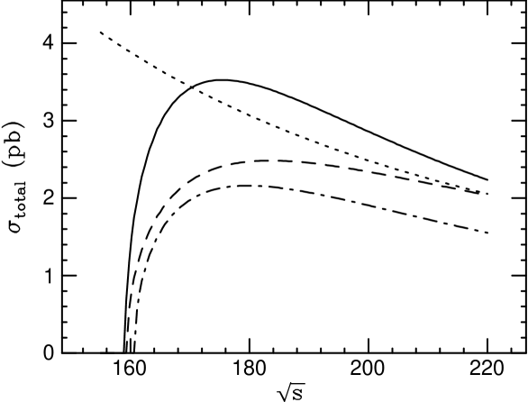
FIG. 1.: The chargino cross section as a function of center-of-mass energy for the three choices of parameters of our case studies: the gaugino case [solid line, see Eq. (13)], the Higgsino case [dashed line, see Eq. (18)], and the mixed case [dot-dashed line, see Eq. (23)]. A unit of R is also shown (dotted line).

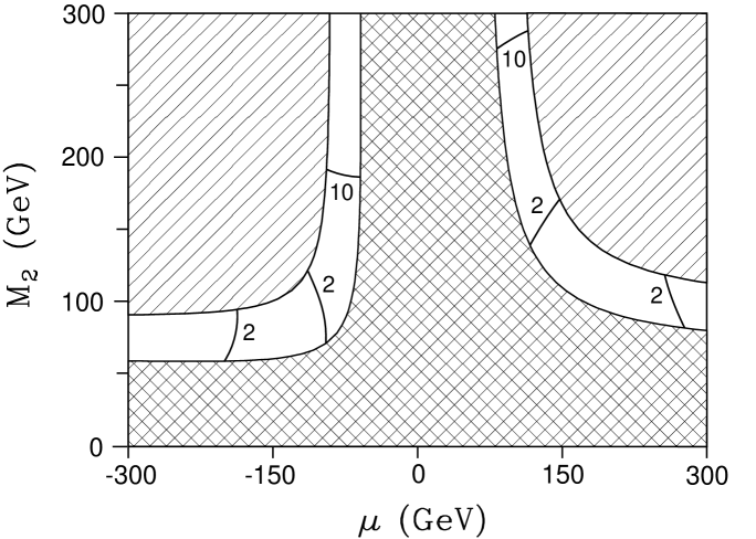
FIG. 2.: Contours of constant $\sigma_{R}/\sigma_{L}$ in percent in the $(\mu,M_{2})$ plane for $\tan\beta=4$ and a sneutrino mass $m_{\tilde{\nu}}=150{\rm\,GeV}$, for which the ratio is nearly maximal. The ratio never rises above 15% in the allowed bands, and is approximately 2% in much of the gaugino region. The cross-hatched region is excluded by the current chargino mass bound $m_{\tilde{\chi}^{\pm}_{1}}>65{\rm\,GeV}$ [9], while in the hatched regions, $m_{\tilde{\chi}^{\pm}_{1}}>95{\rm\,GeV}$, so charginos are kinematically inaccessible at LEP II.

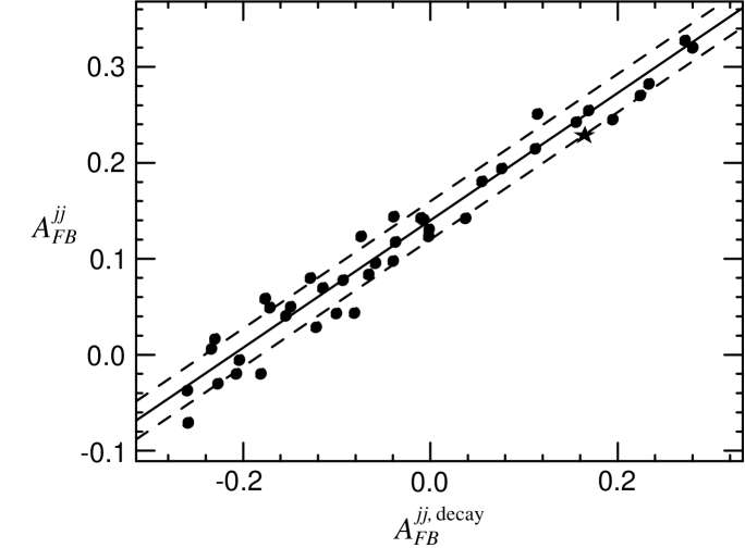
FIG. 3.: Plot of observed $A_{FB}^{jj}$ vs. decay amplitude asymmetry $A_{FB}^{jj,\text{ decay}}$ for numerous points with the same $m_{\tilde{\chi}^{\pm}_{1}}$, $m_{\tilde{\chi}^{0}_{1}}$, $\sigma_{\rm total}$ and $B_{l}$ as the gaugino case study, which is indicated by a star. A linear fit is shown by the solid line with the standard deviation for the fit indicated by the dashed lines.

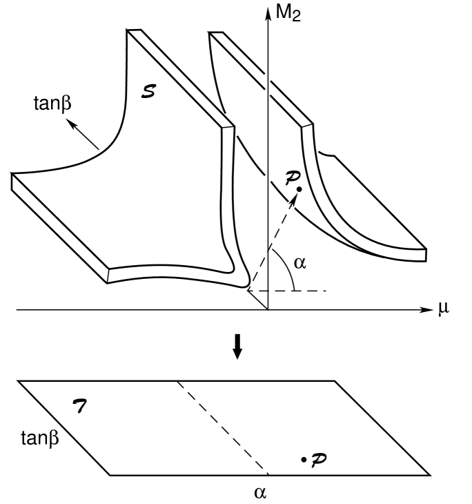
FIG. 4.: The $m_{\tilde{\chi}^{\pm}_{1}}$ measurement restricts the $(\mu,M_{2},\tan\beta)$ space to two thin sheets $\cal S$, which are then flattened into the plane $\cal T$ with the transformation $(\mu,M_{2},\tan\beta)\rightarrow(\alpha,\tan\beta)$, where $\alpha=\arctan(M_{2}/\mu)$. This transformation is illustrated schematically here. For large $\tan\beta$, observables are symmetric under $\mu\leftrightarrow-\mu$, that is, under $\alpha\leftrightarrow 180^{\circ}-\alpha$.

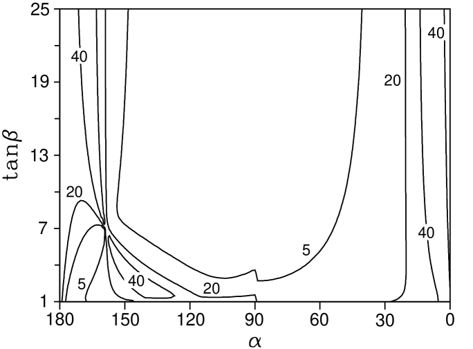
FIG. 5.: Contours of $A_{FB}^{l,\text{ decay}}$ in percent for $M_{1}>0$ and $m_{\tilde{\chi}^{\pm}_{1}}=80{\rm\,GeV}$, $m_{\tilde{\chi}^{0}_{1}}=40{\rm\,GeV}$, $m_{\tilde{l}}=200{\rm\,GeV}$, plotted in the $(\alpha,\tan\beta)$ plane, as defined in Sec. V C.

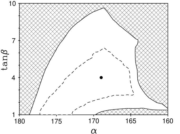
FIG. 6.: Plot of the allowed region (defined in Sec. V C) for the gaugino case study and $M_{1}>0$. The dashed (solid) contour is the projection of the region of parameter space in which all observables are within one (two) standard deviation(s) of their central values; see Sec. V C for discussion. The dot indicates the value of $(\alpha,\tan\beta)$ for the case study.

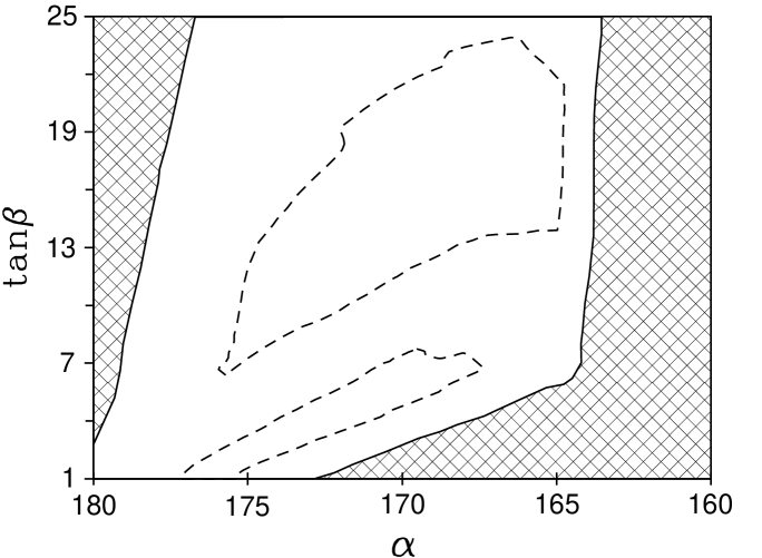
FIG. 7.: Same as Fig. 6 but for $M_{1}<0$. The outer region (solid contour) extends to $\tan\beta=38$.

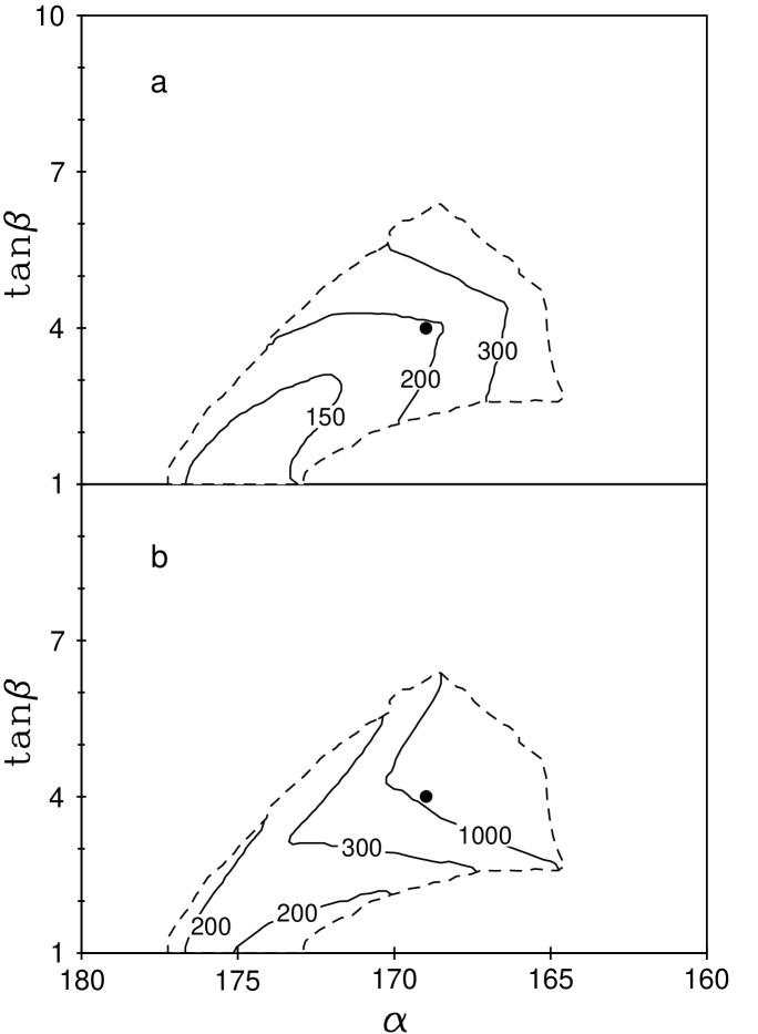
FIG. 8.: Contours of the (a) minimum and (b) maximum values of $m_{\tilde{q}}$ in the $(\alpha,\tan\beta)$ plane, as defined in Sec. V C, for the gaugino case study and $M_{1}>0$, shown only inside the inner allowed region. This illustrates the correlation between $m_{\tilde{q}}$, $\alpha$ and $\tan\beta$. The dot indicates the value of $(\alpha,\tan\beta)$ for the case study.

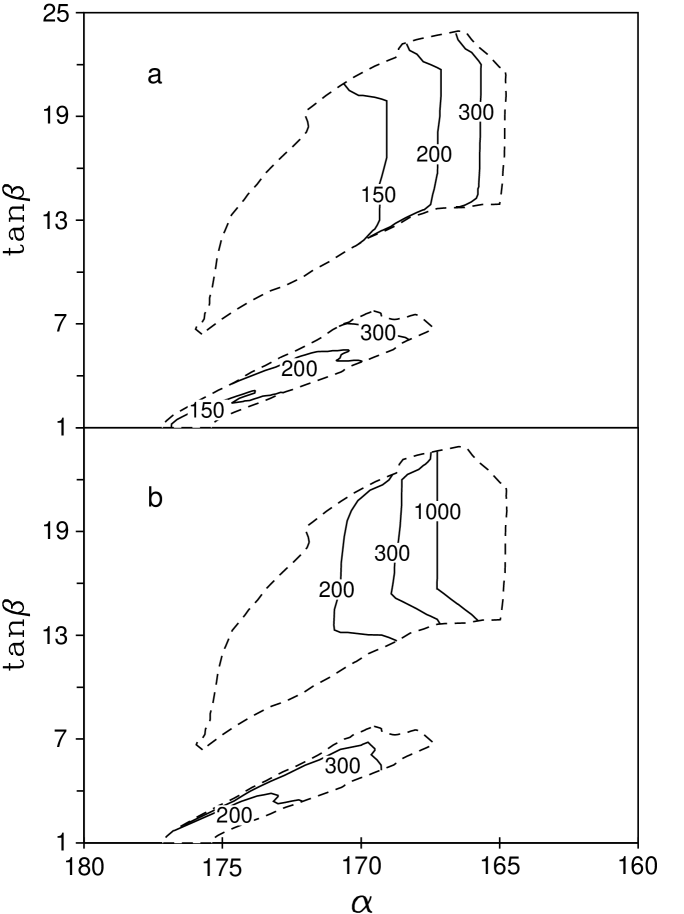
FIG. 9.: Same as Fig. 8 but for $M_{1}<0$.

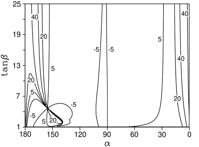
FIG. 10.: Contours of $A_{FB}^{l,\text{ decay}}$ in percent for $M_{1}>0$ and $m_{\tilde{\chi}^{\pm}_{1}}=80{\rm\,GeV}$, $m_{\tilde{\chi}^{0}_{1}}=62{\rm\,GeV}$, $m_{\tilde{l}}=175{\rm\,GeV}$, plotted in the $(\alpha,\tan\beta)$ plane, as defined in Sec. V C.

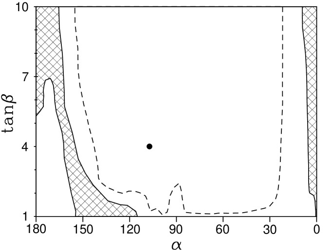
FIG. 11.: Plot of the allowed region (defined in Sec. V C) for the Higgsino case study and $M_{1}>0$. The dashed (solid) contour is the projection of the region of parameter space in which all observables are within one (two) standard deviation(s) of their central values; see Sec. V C for discussion. The dot indicates the value of $(\alpha,\tan\beta)$ for the case study.

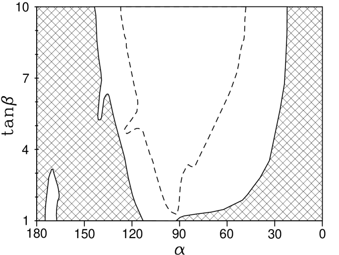
FIG. 12.: Same as Fig. 11 but for $M_{1}<0$.

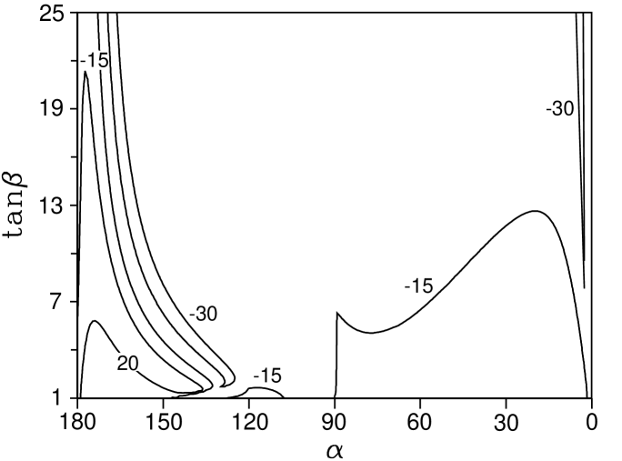
FIG. 13.: Contours of $A_{FB}^{jj,\text{ decay}}$ in percent for $M_{1}>0$ and $m_{\tilde{\chi}^{\pm}_{1}}=80{\rm\,GeV}$, $m_{\tilde{\chi}^{0}_{1}}=53{\rm\,GeV}$, $m_{\tilde{q}}=300{\rm\,GeV}$, plotted in the $(\alpha,\tan\beta)$ plane, as defined in Sec. V C. Jumps in the contours across $\alpha=90^{\circ}$ are due to the discontinuity in the underlying parameters across this line; see Fig. 4.

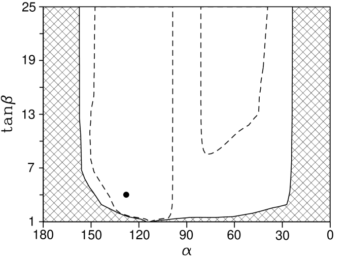
FIG. 14.: Plot of the allowed region (defined in Sec. V C) for the mixed case study and $M_{1}>0$. The dashed (solid) contour is the projection of the region of parameter space in which all observables are within one (two) standard deviation(s) of their central values; see Sec. V C for discussion. The dot indicates the value of $(\alpha,\tan\beta)$ for the case study.

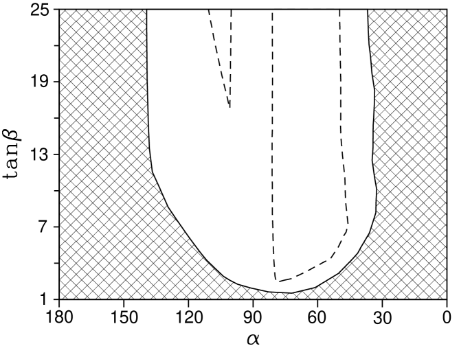
FIG. 15.: Same as Fig. 14 but for $M_{1}<0$. The approximate symmetry $\alpha\leftrightarrow 180^{\circ}-\alpha\$ ($\mu\leftrightarrow-\mu$) for large $\tan\beta$ only becomes evident near $\tan\beta=50$.

REFERENCES

- [1] Physics at LEP2, edited by G. Altarelli, T. Sjöstrand, and F. Zwirner, Vol. I, CERN Report No. CERN–96–01, 1996.
- [2] For reviews of supersymmetry and the minimal supersymmetric standard model, see H.E. Haber and G.L. Kane, Phys. Rep. 117, 75 (1985); H.P. Nilles, Phys. Rep. 110, 1 (1984); P. Nath, R. Arnowitt, and A.H. Chamseddine, Applied Supergravity, ICTP Series in Theoretical Physics, Vol. 1 (World Scientific, Singapore, 1984); X. Tata, in The Standard Model and Beyond, proceedings of the Ninth Symposium on Theoretical Physics, Mt. Sorak, Korea, 1990, edited by J.E. Kim (World Scientific, River Edge, New Jersey, 1991), p. 304.
- [3] For a discussion of mass spectra resulting from different types of SUSY breaking see M.E. Peskin, SLAC Report No. SLAC–PUB–7133, April 1996, hep-ph/9604339, and references therein, to be published in the proceedings of Yukawa International Seminar ’95: From the Standard Model to Grand Unified Theories, Kyoto, Japan, Aug 1995.
- [4] J.L. Feng and M.J. Strassler, Phys. Rev. D 51, 4661 (1995), hep-ph/9408359.
- [5] A. Leike, Int. J. Mod. Phys. A3, 2895 (1988).
- [6] M.A. Diaz and S.F. King, Phys. Lett. B 349, 105 (1995), hep-ph/9501228; Phys. Lett. B 373, 100 (1996), hep-ph/9601230.
- [7] P. Chiappetta, F. M. Renard, J. Soffer, P. Sorba, and P. Taxil, Nucl. Phys. B262, 495 (1985); B279, 824(E) (1987).
- [8] A. Leike, Int. J. Mod. Phys. A4, 845 (1989).
- [9] ALEPH Collaboration, D. Buskulic et al., Phys. Lett. B 373, 246 (1996), CERN Report CERN–PPE–96–010, 1996; OPAL Collaboration, G. Alexander et al., CERN Report CERN–PPE–96–020, 1996; L3 Collaboration, M. Acciarri et al., CERN Report CERN–PPE–96–029, 1996; DELPHI Collaboration, P. Abreu et al., CERN Report CERN–PPE–96–075, 1996.
- [10] N. Oshimo and Y. Kizukuri, Phys. Lett. B 186, 217 (1987).
- [11] C. Dionisi et al., in Proceedings of the ECFA Workshop on LEP 200, Aachen, Federal Republic of Germany, 29 September – 1 October 1986, edited by A. Böhm and W. Hoogland, Vol. II, CERN Report No. 87–08, June 1987, p. 380.
- [12] M. Chen, C. Dionisi, M. Martinez, and X. Tata, Phys. Rep. 159, 201 (1988).
- [13] J.-F. Grivaz, in Proceedings of INFN Eloisatron Project Workshop, Twenty-third: The Decay Properties of SUSY Particles, Erice, Italy, September 28 – October 4, 1992, edited by L. Cifarelli and V. A. Khoze (World Scientific, River Edge, New Jersey, 1993).
- [14] S. Park, Search for New Phenomena in CDF — I: Z’, W’ and Leptoquarks, FERMILAB–CONF–95/155–E. Published Proceedings 10th Topical Workshop on Proton-Antiproton Collider Physics, Fermi National Accelerator Laboratory, Batavia, IL, May 1995.
- [15] D.R. Stump, M. Wiest, and C.P. Yuan, MSUHEP–60116, hep-ph/9601362; S. Dimopoulos, M. Dine, S. Raby and S. Thomas, Phys. Rev. Lett. 76, 3494 (1996); S. Ambrosanio, G.L. Kane, G.D. Kribs, S.P. Martin, S. Mrenna Phys. Rev. Lett. 76, 3498 (1996).
- [16] J.L. Feng, M.E. Peskin, H. Murayama and X. Tata, Phys. Rev. D 52, 1418 (1995), hep-ph/9502260.
- [17] A. Bartl, H. Fraas, and W. Majerotto, Z. Phys. C 30, 441 (1986).
- [18] A. Bartl, H. Fraas, W. Majerotto, and B. Mösslacher, Z. Phys. C 55, 257 (1992).
- [19] C. Ahn et al., SLAC Report No. 329, 1988 (unpublished).
- [20] J.F. Gunion and H.E. Haber, Nucl. Phys. B272, 1 (1986); B402, 567(E) (1993).
- [21] L. Girardello and M.T. Grisaru, Nucl. Phys. B194, 65 (1982).