QCD resummation and heavy quark cross sections

Abstract

In this dissertation a detailed analysis of heavy quark production is given with an emphasis on the resummation of soft gluon corrections.

First we calculate the production cross sections for top quark production at the Fermilab Tevatron and for bottom quark production at fixed-target $pp$ experiments, and in particular HERA-B. We consider both the order $\alpha_{s}^{3}$ cross sections and the resummation of soft gluon corrections in all orders of QCD perturbation theory.

Then we calculate the inclusive transverse momentum and rapidity distributions for top quark production at the Fermilab Tevatron and bottom quark production at HERA-B. We give both $\alpha_{s}^{3}$ and resummed results.

Finally, we discuss the resummation of distributions that are singular at the elastic limit of partonic phase space (partonic threshold) in QCD hard-scattering cross sections, such as heavy quark production. We show how nonleading soft logarithms exponentiate in a manner that depends on the color structure within the underlying hard scattering. This result generalizes the resummation of threshold singularities for the Drell-Yan process, in which the hard scattering proceeds through color-singlet annihilation. We illustrate our results for the case of heavy quark production by light quark annihilation and gluon fusion, and also for light quark production through gluon fusion.

We, the dissertation committee for the above candidate for the Doctor of Philosophy degree, hereby recommend acceptance of the dissertation.

This dissertation is accepted by the Graduate School.

 

Graduate School

For Natalia and my parents

Contents

toc

List of Figures

lof

Chapter 1 Introduction

In this dissertation we will be concerned with the calculation of heavy quark cross sections and differential distributions in transverse momentum and rapidity. In particular we will examine top quark production at the Fermilab Tevatron and bottom quark production at fixed target $pp$ experiments and HERA-B.

The Standard Model of Particle Physics is at present the most successful model for the description of the interactions of elementary particles. In this model all the fundamental interactions derive from the principle of local gauge invariance. The Standard Model is described by the gauge group $SU(3)_{C}\otimes SU(2)_{L}\otimes U(1)_{Y}$, which incorporates the Glashow-Weinberg-Salam theory of electroweak processes and Quantum Chromodynamics (QCD). QCD is the local $SU(3)_{C}$ gauge field theory of strong interactions and in perturbative QCD we make physical predictions by expanding in powers of the strong coupling constant $\alpha_{s}$.

In the Standard Model there are three families of quarks and leptons. The heaviest family of quarks consists of the top and the bottom quarks. The latter was discovered in the seventies but the top was elusive until recently due to its very high mass. The search for the top has gone on for more than a decade with experimental groups continually establishing ever higher limits for the top quark mass. The recent discovery of the top quark by the two experimental groups CDF [1] and D0 [2] at the Fermilab Tevatron has been the biggest discovery in particle physics in the last decade and has given us one more confirmation of the Standard Model. The existence of the top was expected on theoretical grounds for the cancellation of anomalies. CDF announced a top quark mass of $176\pm 8\pm 10$ GeV/$c^{2}$ and a $t\bar{t}$ production cross section of $6.8^{+3.6}_{-2.4}$ pb. D0 measured the top quark mass to be $199^{+19}_{-21}\pm 22$ GeV/$c^{2}$ and its production cross section to be $6.4\pm 2.2$ pb.

Perturbative QCD (pQCD) is applicable only at high energies since it is only in this domain that $\alpha_{s}$ is small according to the principle of asymptotic freedom [3]. The expansion of $\alpha_{s}$ in the renormalization scale $\mu$ is given by

$$\alpha_{s}(\mu^{2},n_{f})=\frac{12\pi}{(33-2n_{f})\ln(\mu^{2}/\Lambda^{2})}\left[1-\frac{6(153-19n_{f})}{(33-2n_{f})^{2}}\frac{\ln(\ln(\mu^{2}/\Lambda^{2}))}{\ln(\mu^{2}/\Lambda^{2})}\right]+\cdots$$ (1.1)

where $n_{f}$ is the number of quarks with mass less than $\mu$ and $\Lambda$ is the QCD scale parameter.

Figure 1.1: The strong coupling constant $\alpha_{s}$ versus scale

In fig. 1 we plot $\alpha_{s}$ as a function of scale. We see that at the scale relevant to top quark production (i.e. the top quark mass, which we take to be 175 GeV/$c^{2}$) the value of the coupling is about 0.1. This number is small enough to allow perturbative QCD calculations to be reliable. For bottom quark production the relevant scale is the bottom quark mass (which we take to be 4.75 GeV/$c^{2}$). There the value of the coupling is about 0.2, which is still small but not as much as for the top quark case.

The calculation of production cross sections for heavy particles in QCD is made by invoking the factorization theorem [4] and expanding the contributions to the amplitude in powers of the coupling constant $\alpha_{s}(\mu^{2})$. One has to perform both renormalization of ultraviolet divergences and mass factorization of collinear divergences. In top and bottom quark production the heavy quark-antiquark pairs are created in parton-parton collisions. For the Born $O(\alpha_{s}^{2})$ cross section the two relevant processes are quark-antiquark annihilation

$$q+{\bar{q}}\rightarrow Q+{\bar{Q}},$$ (1.2)

and gluon-gluon fusion

$$g+g\rightarrow Q+{\bar{Q}}.$$ (1.3)

In $O(\alpha_{s}^{3})$ the relevant parton-parton processes are

$$q+{\bar{q}}\rightarrow Q+{\bar{Q}}+g,$$ (1.4)

$$g+g\rightarrow Q+{\bar{Q}}+g,$$ (1.5)

$$q+g\rightarrow Q+{\bar{Q}}+q,$$ (1.6)

$${\bar{q}}+g\rightarrow Q+{\bar{Q}}+{\bar{q}},$$ (1.7)

together with the virtual corrections to (1.2) and (1.3). Recent investigations have shown that near threshold there are large logarithms in the perturbation expansion which have to be resummed to make more reliable theoretical predictions. The standard process is fixed target Drell-Yan production, which has been the subject of many papers over the past few years [5]. The same ideas on resummation were applied to the calculation of the top-quark cross section at the Fermilab Tevatron in [6] and [7]. What is relevant in these reactions is the existence of a class of logarithms of the type $(\ln(1-z))^{i}/(1-z)$, where $i$ is the order of the perturbation expansion, and where one must integrate over the variable $z$ up to a limit $z=1$. These terms are not actually singular at $z=1$ due to the presence of terms in $\delta(1-z)$. However the remainder can be quite large. In general one writes such terms as “plus” distributions, which are then convoluted with regular test functions (the parton densities).

In perturbation theory with a hard scale we can use the standard expression for the order-by order cross section in QCD, namely

$$\sigma(S,m^{2}) = \int_{\frac{4m^{2}}{S}}^{1}dx_{1}\int_{\frac{4m^{2}}{x_{1}S}}^{1}dx_{2}\sum_{ij}f_{i}(x_{1},\mu^{2})f_{j}(x_{2},\mu^{2})\sigma_{ij}(s=x_{1}x_{2}S,m^{2},\mu^{2})\,,$$

where the $f_{i}(x,\mu^{2})$ are the parton densities at the factorization scale $\mu^{2}$ and the $\sigma_{ij}$ are the partonic cross sections. The numerical results for the hadronic cross sections depend on the choice of the parton densities, which involves the mass factorization scale $\mu^{2}$; the choice of the running coupling constant, which involves the renormalization scale (also normally chosen to be $\mu^{2}$); and the choice for the actual mass of the heavy quark. In lowest order or Born approximation the actual numbers for the cross section show a large sensitivity to these parameters. In chapter 2 we will show plots of the top and bottom quark production cross sections in leading order (LO), i.e. $O(\alpha_{s}^{2})$, and next-to-leading order (NLO), i.e. $O(\alpha_{s}^{3})$. The NLO results follow from the work of the two groups [8] and [9]. However even including the NLO corrections does not completely fix the cross section. The sensitivity to our lack of knowledge of even higher terms in the QCD expansion is usually demonstrated by varying the scale choice up and down by factors of two. In general it is impossible to make more precise predictions given the absence of a calculation in next-to-next-to-leading order (NNLO). However in specific kinematical regions we can do so.

The threshold region is one of these regions. In this region one finds that there are large logarithms which arise from an imperfect cancellation of the soft-plus-virtual (S+V) terms in the perturbation expansion. These logarithms are exactly of the same type mentioned above. In [6] the dominant logarithms from initial state gluon bremsstrahlung (ISGB), which are the cause of the large corrections near threshold, were carefully examined. Such logarithms have been studied previously in Drell-Yan (DY) [5] production at fixed target energies (again near threshold) where they are responsible for correspondingly large corrections. The analogy between DY and heavy quark production cross sections was exploited in [6] and a formula to resum the leading logarithms in pQCD to all orders was proposed. Since the contributions due to these logarithms are positive (when all scales $\mu$ are set equal to the heavy quark mass $m$), the effect of summing the higher order corrections increases the top and bottom quark production cross sections over those predicted in $O(\alpha_{s}^{3})$. This sum, which will be identified as $\sigma_{\rm res}$, depends on a nonperturbative parameter $\mu_{0}$. The reason that a new parameter has to be introduced is that the resummation is sensitive to the scale at which pQCD breaks down. As we approach the threshold region other, nonperturbative, physics plays a role (higher twist, bound states, etc.) indicated by a dramatic increase in $\alpha_{s}$ and in the resummed cross section. This is commonly called the effect of the infrared renormalon or Landau pole [10]. We choose to simply cut off the resummation at a specific scale $\mu_{0}$ where $\Lambda<<\mu_{0}<<m$ since it is not obvious how to incorporate the nonperturbative effects. Note that our resummed corrections diverge for small $\mu_{0}$ but this is not physical since they should be joined smoothly onto some nonperturbative prescription and the total cross section will be finite. Another way to make it finite would be to avoid the infrared renormalon by a specific continuation around it, i.e. the principal value resummation method [11]. However, at the moment our total resummed corrections depend on the parameter $\mu_{0}$ for which we can only make a rough estimate.

We will see in chapter 2 that the gluon-gluon channel is the dominant channel for the production of $b$-quarks near threshold in a fixed-target $pp$ experiment. This is not the case for the production of the top quark at the Fermilab Tevatron, which is a proton-antiproton collider, and where the dominant channel is the quark-antiquark one. That was fortunate as the exponentiation of the soft-plus-virtual terms in [6] is on a much more solid footing in the $q\bar{q}$ channel, due to all the past work which has been done on the Drell-Yan reaction [5]. We will examine all “large” corrections near threshold, including both Coulomb-like and large constant terms. We will do that in chapter 2 where we will present all the relevant formulae at the partonic level. In addition we will present subleading S+V terms and discuss their contribution to the total S+V cross section. Chapter 2 also contains the analysis of the hadron-hadron cross section which is relevant for top quark production at the Fermilab Tevatron as well as for bottom quark production for the HERA-B experiment and for fixed-target $pp$ experiments in general. We give results in LO, in NLO and after resummation. Most of our results in chapter 2 have appeared in [12] and [13].

In chapter 3 we will present results for the heavy quark differential distributions in transverse momentum $p_{T}$ and rapidity $Y$. After showing the relevant formulas at the partonic level and discussing resummation we will give results for top and bottom quark production at the Fermilab Tevatron and HERA-B, respectively. We will show that resummation produces an enhancement of the NLO results with little change in shape. Our results in this chapter have appeared in [12] and [14].

In chapter 4 we will present a new resummation formula that takes into account subleading logarithms. A strong motivation for this research is the inadequacy of the leading-log approximation for the $gg$ channel as will be discussed in chapter 2. We will show how nonleading soft logarithms exponentiate in a manner that depends on the color structure within the underlying hard scattering. We will derive the anomalous dimension matrices and exhibit the exponentiation of nonleading soft logarithms for the production of heavy quarks through both light quark-antiquark annihilation and gluon-gluon fusion. Some of our results in chapter 4 have been presented in [15].

Chapter 2 Top and bottom quark production cross sections

In this chapter we present general formulas for heavy quark cross sections. First we discuss our results at the partonic level and then we give the calculations for the cross sections for top quark production at the Fermilab Tevatron and for bottom quark production at fixed-target energies and HERA-B. We present both the order $\alpha_{s}^{3}$ cross sections and the resummation of soft gluon corrections in all orders of QCD perturbation theory.

2.1 Results for parton-parton reactions

The partonic processes that we examine are

$$i(k_{1})+j(k_{2})\rightarrow Q(p_{1})+\bar{Q}(p_{2}),$$ (2.1.1)

where $i,j=g,q,\bar{q}$. The square of the parton-parton center-of-mass (c.m.) energy is $s=(k_{1}+k_{2})^{2}$.

We begin with an analysis of heavy quark production in the $q\bar{q}$ channel. The Born cross section in this channel is given by

$$\sigma_{q\bar{q}}^{(0)}(s,m^{2})=\frac{2\pi}{3}\alpha_{s}^{2}(\mu^{2})K_{q\bar{q}}NC_{F}\frac{1}{s}\beta\left(1+\frac{2m^{2}}{s}\right)$$ (2.1.2)

where $C_{F}=(N^{2}-1)/(2N)$ is the Casimir invariant for the fundamental representation of $SU(N)$, $K_{q\bar{q}}=N^{-2}$ is a color average factor, $\mu$ denotes the renormalization scale, and $\beta=\sqrt{1-4m^{2}/s}$. Also $N=3$ for the $SU(3)$ color group in QCD. The threshold behavior ($s\rightarrow 4m^{2}$) of this expression is given by

$$\sigma_{q\bar{q},\,\rm thres}^{(0)}(s,m^{2})=\pi\alpha_{s}^{2}(\mu^{2})K_{q\bar{q}}NC_{F}\frac{1}{s}\beta.$$ (2.1.3)

Complete analytic results are not available for the NLO cross section as some integrals are too complicated to do by hand. However in [1] analytic results are given for the soft-plus-virtual (S+V) contributions to the cross section, and for the approximation to the cross section near threshold. Simple formulas which yield reasonable approximations to the exact $O(\alpha_{s}^{3})$ results have been constructed in [2]. From these results one can derive that the Coulomb terms to first order in the $q\bar{q}$ channel are given by

$$\sigma^{(\pi^{2})}_{q\bar{q}}(s,m^{2})=\sigma^{(0)}_{q\bar{q}}(s,m^{2})\frac{\pi\alpha_{s}(\mu^{2})}{2\beta}\left(C_{F}-\frac{C_{A}}{2}\right)$$ (2.1.4)

in the $\overline{\rm MS}$ scheme, where $C_{A}=N$ is the Casimir invariant for the adjoint representation of $SU(N)$. These terms are distinguished by their typical $\beta^{-1}$ behavior near threshold which, after multiplication by the Born cross section, yield finite cross sections at threshold in NLO. We note that $C_{F}-C_{A}/2=-1/6$ is negative for $SU(3)$ and that the first-order Coulomb correction is negative (the interaction is repulsive).

In the DIS scheme, in addition to the Coulomb terms, we also have a large constant contribution so that the first order result near threshold is

$$\sigma^{(\pi^{2})}_{q\bar{q}}(s,m^{2})=\sigma^{(0)}_{q\bar{q}}(s,m^{2})\left[\frac{\pi\alpha_{s}(\mu^{2})}{2\beta}\left(C_{F}-\frac{C_{A}}{2}\right)+\frac{\alpha_{s}(\mu^{2})}{\pi}C_{F}\left(\frac{9}{2}+\frac{\pi^{2}}{3}\right)\right].$$ (2.1.5)

We have included the constant terms to see their effect at larger values of $\beta$.

Since the total parton-parton cross sections only depend on the variables $s$ and $m^{2}$ they can be expressed in terms of scaling functions as follows

$$\sigma_{ij}(s,m^{2}) = \sum_{k=0}^{\infty}\sigma_{ij}^{(k)}(s,m^{2})$$ (2.1.6)

$$= \frac{\alpha_{s}^{2}(\mu^{2})}{m^{2}}\sum_{k=0}^{\infty}(4\pi\alpha_{s}(\mu^{2}))^{k}\sum_{l=0}^{k}f_{ij}^{(k,l)}(\eta)\ln^{l}\frac{\mu^{2}}{m^{2}},$$

where we denote by $\sigma^{(k)}$ the $O(\alpha_{s}^{k+2})$ contribution to the cross section. The scaling functions $f_{ij}^{(k,l)}(\eta)$ depend on the scaling variable $\eta=s/4m^{2}-1=s\beta^{2}/4m^{2}$.

Figure 2.1: The scaling functions $f_{q\bar{q}}^{(k,0)}$ in the $\overline{\rm MS}$ scheme. Plotted are $f_{q\bar{q}}^{(0,0)}$ (exact, upper solid line at large $\eta$; threshold approximation, upper dotted line at large $\eta$), $f_{q\bar{q}}^{(1,0)}$ (exact, lower solid line at large $\eta$; threshold approximation, lower dotted line at large $\eta$).

In fig. 2.1 we plot $f_{q\bar{q}}^{(k,0)}(\eta)$ for $k=0,1$ for the exact and threshold expressions (from [1]) in the $\overline{\rm MS}$ scheme. We see that the threshold Born approximation is excellent for small $\eta$ and reasonable for the entire range of $\eta$ shown. We also note that the theshold first-order approximation is good only very near to threshold.

Figure 2.2: Same as fig. 2.1 but now for the DIS scheme.

In fig. 2.2 we plot the corresponding functions for the DIS scheme. Here the first-order corrections are smaller than in the $\overline{\rm MS}$ scheme. Again the threshold first-order approximation is good only very close to threshold.

The analysis of the contributions to the gluon-gluon channel in NLO is much more complicated. First of all there are three Born diagrams each with a different color structure. Therefore only few terms near threshold are proportional to the Born cross section. The exact Born term in the $gg$ channel is

$$\sigma_{gg}^{(0)}(s,m^{2}) = 4\pi\alpha_{s}^{2}(\mu^{2})K_{gg}NC_{F}\frac{1}{s}\left\{C_{F}\left[-\left(1+\frac{4m^{2}}{s}\right)\beta\right.\right.$$ (2.1.7)

$$\quad\quad\quad\quad+\left.\left(1+\frac{4m^{2}}{s}-\frac{8m^{4}}{s^{2}}\right)\ln\frac{1+\beta}{1-\beta}\right]$$

$$+\left.C_{A}\left[-\left(\frac{1}{3}+\frac{5}{3}\frac{m^{2}}{s}\right)\beta+\frac{4m^{4}}{s^{2}}\ln\frac{1+\beta}{1-\beta}\right]\right\},$$

where $K_{gg}=(N^{2}-1)^{-2}$ is a color average factor. The threshold behavior ($s\rightarrow 4m^{2}$) of this expression is given by

$$\sigma_{gg,\,\rm thres}^{(0)}(s,m^{2})=\pi\alpha_{s}^{2}(\mu^{2})K_{gg}\frac{1}{s}NC_{F}[4C_{F}-C_{A}]\beta.$$ (2.1.8)

Again, the complete NLO expression for the cross section in the $gg$ channel is unavailable but analytic results are given for the S+V terms in [3]. These were used in [2] to analyze the magnitude of the cross section near threshold. From the approximate expressions given in [2] one can extract the $\pi^{2}$ terms to first order in the $gg$ channel. These are

$$\sigma_{gg}^{(\pi^{2})}(s,m^{2}) = \alpha_{s}^{3}(\mu^{2})NC_{K}K_{gg}\frac{\pi^{2}}{s}\left[\frac{5}{8}+\frac{1}{24}\beta^{2}+16\frac{m^{6}}{s^{3}}\right.$$ (2.1.9)

$$\quad\quad\quad+\left.\left(32\frac{m^{8}}{s^{4}}-10\frac{m^{4}}{s^{2}}\right)\frac{1}{\beta}\ln\frac{1+\beta}{1-\beta}\right]$$

$$+\alpha_{s}^{3}C_{\rm QED}K_{gg}\frac{\pi^{2}}{s}\left[-\frac{1}{4}-16\frac{m^{6}}{s^{3}}\right.$$

$$\quad\quad\quad\left.+\left(-32\frac{m^{8}}{s^{4}}+8\frac{m^{4}}{s^{2}}\right)\frac{1}{\beta}\ln\frac{1+\beta}{1-\beta}\right],$$

where $C_{K}=(N^{2}-1)/N=2NC_{F}C_{A}-4NC_{F}^{2}$, and $C_{\rm QED}=(N^{4}-1)/N^{2}=-4C_{F}^{2}+4C_{A}C_{F}$. These are not proportional to the Born term. The threshold behavior of (2.1.9) is given by

$$\sigma_{gg,\,\rm thres}^{(\pi^{2})}(s,m^{2})=\alpha_{s}^{3}(\mu^{2})K_{gg}\frac{\pi^{2}}{4}\frac{1}{s}\left[\frac{-NC_{K}}{2}+C_{\rm QED}\right],$$ (2.1.10)

which is proportional to the threshold Born term. Therefore the threshold approximation for the $\pi^{2}$ terms in NLO can be written as

$$\sigma_{gg,\,\rm thres}^{(0)+(\pi^{2})}(s,m^{2})=\sigma_{gg,\,\rm thres}^{(0)}(s,m^{2})\left[1+\frac{\pi\alpha_{s}(\mu^{2})}{4\beta}\left(\frac{-NC_{K}/2+C_{\rm QED}}{(4C_{F}-C_{A})NC_{F}}\right)\right],$$ (2.1.11)

or, writing the color factors in terms of $N$, as

$$\sigma_{gg,\,\rm thres}^{(0)+(\pi^{2})}(s,m^{2})=\sigma_{gg,\,\rm thres}^{(0)}(s,m^{2})\left[1+\frac{\pi\alpha_{s}(\mu^{2})}{4\beta}\frac{N^{2}+2}{N(N^{2}-2)}\right].$$ (2.1.12)

Figure 2.3: Same as fig. 2.1 but now for $f_{gg}^{(k,0)}$ in the $\overline{\rm MS}$ scheme.

In fig. 2.3 we plot the scaling functions $f_{gg}^{(k,0)}(\eta)$ with $k=0,1$ in the $\overline{\rm MS}$ scheme for the exact and threshold expressions (from [3]). We see that the Born and first-order threshold approximations are good only very close to threshold.

In [4] an approximation was given for the NLO soft-plus-virtual contributions and the analogy with the Drell-Yan process was exploited to resum them to all orders of perturbation theory. The S+V approximation is adequate in the region $0.1<\eta<1$ (which is the kinematical region of interest as we will see in sections 2.2 and 2.3) for the $q\bar{q}$ channel, but not as good for the $gg$ channel in the $\overline{\rm MS}$ scheme. Therefore we reexamined the approximate formulae given in [2] for the initial state gluon bremsstrahlung (ISGB) mechanism to see if there are subleading terms that will improve the S+V approximation. Let us see the structure of these terms. We are discussing partonic reactions of the type $i(k_{1})+j(k_{2})\rightarrow Q(p_{1})+\bar{Q}(p_{2})+g(k_{3})$, and we introduce the kinematic variables $t_{1}=(k_{2}-p_{2})^{2}-m^{2}$, $u_{1}=(k_{1}-p_{2})^{2}-m^{2}$, and $s_{4}=s+t_{1}+u_{1}$. The variable $s_{4}$ depends on the four-momentum of the extra partons emitted in the reaction. We write the differential cross section in order $\alpha_{s}^{k}(\mu^{2})$ as follows

$$s^{2}\frac{d^{2}\sigma_{ij}^{(k)}(s,t_{1},u_{1})}{dt_{1}\>du_{1}} = \alpha_{s}^{k}(\mu^{2})\sum_{l=0}^{2k-1}\Big{[}\frac{1}{s_{4}}a_{l}(\mu^{2})\ln^{l}\Big{(}\frac{s_{4}}{m^{2}}\Big{)}\theta(s_{4}-\Delta)$$

$$+\frac{1}{l+1}a_{l}(\mu^{2})\ln^{l+1}\Big{(}\frac{\Delta}{m^{2}}\Big{)}\delta(s_{4})\Big{]}\sigma^{B}_{ij}(s,t_{1},u_{1})\,.$$

Here a small parameter $\Delta$ has been introduced to allow us to distinguish between the soft ($s_{4}<\Delta$) and the hard ($s_{4}>\Delta$) regions in phase space. The quantities $a_{l}(\mu^{2})$ contain terms involving the QCD $\beta$-functions and color factors. The variables $t_{1}$ and $u_{1}$ are then mapped onto the variables $s_{4}$ and $\cos\theta$, where $\theta$ is the parton-parton c.m. scattering angle:

$$t_{1} = -\frac{1}{2}\left\{s-s_{4}-[(s-s_{4})^{2}-4sm^{2}]^{1/2}\cos\theta\right\},$$ (2.1.14)

$$u_{1} = -\frac{1}{2}\left\{s-s_{4}+[(s-s_{4})^{2}-4sm^{2}]^{1/2}\cos\theta\right\}.$$ (2.1.15)

After explicit integration over the angle $\theta$, the series becomes

$$\sigma_{ij}^{(k)}(s,m^{2}) = \alpha_{s}^{(k)}(\mu^{2})\sum_{l=0}^{2k-1}a_{l}(\mu^{2})\left\{\int_{0}^{s-2ms^{1/2}}ds_{4}\frac{1}{s_{4}}\ln^{l}\frac{s_{4}}{m^{2}}\right.$$ (2.1.16)

$$\times[{\bar{\sigma}}_{ij}^{(0)}(s,s_{4},m^{2})-{\bar{\sigma}}_{ij}^{(0)}(s,0,m^{2})]$$

$$\left.+\frac{1}{l+1}\ln^{l+1}\left(\frac{s-2ms^{1/2}}{m^{2}}\right){\bar{\sigma}}_{ij}^{(0)}(s,0,m^{2})\right\},$$

where

$${\bar{\sigma}}_{ij}^{(0)}(s,s_{4},m^{2})=\frac{1}{2s^{2}}[(s-s_{4})^{2}-4sm^{2}]^{1/2}\int_{-1}^{1}d\cos\theta\;\;\sigma_{ij}^{B}(s,s_{4},\cos\theta).$$ (2.1.17)

The Born approximation differential cross sections can be expressed by

$$s^{2}\frac{d^{2}\sigma^{(0)}_{ij}(s,t_{1},u_{1})}{dt_{1}\>du_{1}}=\delta(s+t_{1}+u_{1})\,\sigma^{B}_{ij}(s,t_{1},u_{1})\,,$$ (2.1.18)

with

$$\sigma^{B}_{q\bar{q}}(s,t_{1},u_{1})=\pi\alpha_{s}^{2}(\mu^{2})K_{q\bar{q}}NC_{F}\Big{[}\frac{t_{1}^{2}+u_{1}^{2}}{s^{2}}+\frac{2m^{2}}{s}\Big{]}\,,$$ (2.1.19)

and

$$\sigma^{B}_{gg}(s,t_{1},u_{1}) = 2\pi\alpha_{s}^{2}(\mu^{2})K_{gg}NC_{F}\Big{[}C_{F}-C_{A}\frac{t_{1}u_{1}}{s^{2}}\Big{]}$$ (2.1.20)

$$\times\Big{[}\frac{t_{1}}{u_{1}}+\frac{u_{1}}{t_{1}}+\frac{4m^{2}s}{t_{1}u_{1}}\Big{(}1-\frac{m^{2}s}{t_{1}u_{1}}\Big{)}\Big{]}\,.$$

The first-order approximate S+V result for the $q\bar{q}$ channel in the $\overline{\rm MS}$ scheme is

$$s^{2}\frac{d^{2}\sigma^{(1)}_{q\bar{q}}(s,t_{1},u_{1})}{dt_{1}du_{1}} = \sigma_{q\bar{q}}^{B}(s,t_{1},u_{1})\frac{2C_{F}}{\pi}\alpha_{s}(\mu^{2})$$

$$\times\left\{\left[\frac{1}{s_{4}}\left(2\ln\frac{s_{4}}{m^{2}}+\ln\frac{m^{2}}{\mu^{2}}\right)\theta(s_{4}-\Delta)\right.\right.$$

$$\left.+\left(\ln^{2}\frac{\Delta}{m^{2}}+\ln\frac{\Delta}{m^{2}}\ln\frac{m^{2}}{\mu^{2}}\right)\delta(s_{4})\right]$$

$$+\left.\left[-\frac{C_{A}}{2C_{F}}\frac{1}{s_{4}}\theta(s_{4}-\Delta)-\frac{C_{A}}{2C_{F}}\ln\frac{\Delta}{m^{2}}\delta(s_{4})\right]\right\}\,.$$

The terms in the first pair of square brackets in (2.1.21) are the leading S+V terms given in [4] and those in the second pair of square brackets are subleading terms that we want to examine.

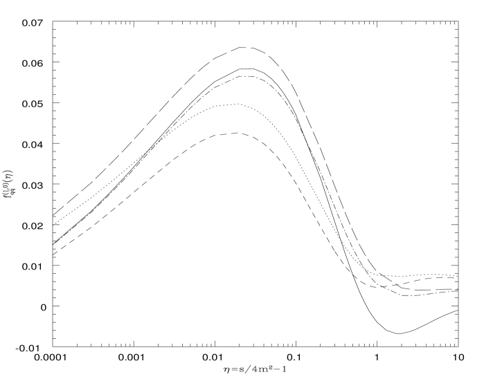
Figure 2.4: The scaling functions $f_{q\bar{q}}^{(1,0)}$ in the $\overline{\rm MS}$ scheme. Plotted are the exact result (solid line), the leading S+V approximation (dotted line), the leading S+V approximation plus Coulomb terms (short-dashed line), the S+V approximation with leading plus subleading terms (long dashed line), and the S+V approximation with leading plus subleading terms plus Coulomb terms (dash-dotted line).

In fig. 2.4 we plot the scaling functions $f_{q\bar{q}}^{(1,0)}$ for the exact result, the leading approximate S+V result, and the approximate S+V result with both leading and subleading logarithms. The leading S+V result is a reasonable approximation to the exact result in our region of interest $0.1<\eta<1$. The addition of Coulomb terms worsens the leading S+V result. We also see that when we include the subleading terms our approximation does not improve much in the region of interest. However, when we add both the first order Coulomb terms and subleading terms to the leading S+V result we get a very good agreement with the exact result. In the DIS scheme the analogous results are

$$s^{2}\frac{d^{2}\sigma^{(1)}_{q\bar{q}}}{dt_{1}du_{1}}(s,t_{1},u_{1}) = \sigma_{q\bar{q}}^{B}(s,t_{1},u_{1})\frac{2C_{F}}{\pi}\alpha_{s}(\mu^{2})$$ (2.1.22)

$$\times\left\{\left[\frac{1}{s_{4}}\left(\ln\frac{s_{4}}{m^{2}}+\ln\frac{m^{2}}{\mu^{2}}\right)\theta(s_{4}-\Delta)\right.\right.$$

$$\left.+\left(\frac{1}{2}\ln^{2}\frac{\Delta}{m^{2}}+\ln\frac{\Delta}{m^{2}}\ln\frac{m^{2}}{\mu^{2}}\right)\delta(s_{4})\right]$$

$$+\left[\left(\frac{3}{4}+\ln 2-\frac{C_{A}}{2C_{F}}\right)\frac{1}{s_{4}}\theta(s_{4}-\Delta)\right.$$

$$\left.\left.+\left(\frac{3}{4}+\ln 2-\frac{C_{A}}{2C_{F}}\right)\ln\frac{\Delta}{m^{2}}\delta(s_{4})\right]\right\}.$$

Figure 2.5: Same af fig. 2.4 but now for the DIS scheme.

In fig. 2.5 we plot the corresponding scaling functions. Here the addition of subleading terms worsens the leading S+V approximation. The addition of Coulomb terms and large constants enhances the first-order approximate results considerably.

The resummation of the leading S+V terms has been given in [4]. The result is

$$s^{2}\frac{d^{2}\sigma^{\rm res}_{q\bar{q}}(s,t_{1},u_{1})}{dt_{1}du_{1}} = \sigma_{q\bar{q}}^{B}(s,t_{1},u_{1})\left[\frac{df(s_{4}/m^{2},m^{2}/\mu^{2})}{ds_{4}}\theta(s_{4}-\Delta)\right.$$ (2.1.23)

$$\quad\quad\quad\quad\quad\quad+\left.f(\frac{\Delta}{m^{2}},\frac{m^{2}}{\mu^{2}})\delta(s_{4})\right],$$

where

$$f\left(\frac{s_{4}}{m^{2}},\frac{m^{2}}{\mu^{2}}\right)=\exp\left[A\frac{C_{F}}{\pi}\bar{\alpha}_{s}\left(\frac{s_{4}}{m^{2}},m^{2}\right)\ln^{2}\frac{s_{4}}{m^{2}}\right]\frac{[s_{4}/m^{2}]^{\eta}}{\Gamma(1+\eta)}\exp(-\eta\gamma_{E}).$$ (2.1.24)

The straightforward expansion of the exponential plus the change of the argument in $\bar{\alpha}_{s}$ via the renormalization group equations generates the corresponding leading logarithmic terms. The scheme dependent $A$ and $\bar{\alpha}_{s}$ in the above expression are given by

$$A=2,\;\;\;\;\;\bar{\alpha}_{s}(y,\mu^{2})=\alpha_{s}(y^{2/3}\mu^{2})=\frac{4\pi}{\beta_{0}\ln(y^{2/3}\mu^{2}/\Lambda^{2})}\,,$$ (2.1.25)

in the $\overline{\rm MS}$ scheme, and

$$\!\!\!\!\!\!\!\!\!\!\!\!A=1,\;\;\;\;\;\bar{\alpha}_{s}(y,\mu^{2})=\alpha_{s}(y\mu^{2})=\frac{4\pi}{\beta_{0}\ln(y\mu^{2}/\Lambda^{2})}\,,$$ (2.1.26)

in the DIS scheme, where $\beta_{0}=11/3\;C_{A}-2/3\;n_{f}$ is the lowest order coefficient of the QCD $\beta$-function. The color factors $C_{ij}$ are defined by $C_{q\bar{q}}=C_{F}$ and $C_{gg}=C_{A}$, and $\gamma_{E}$ is the Euler constant. The quantity $\eta$ is given by

$$\eta=\frac{8C_{ij}}{\beta_{0}}\ln\left(1+\beta_{0}\frac{\alpha_{s}(\mu^{2})}{4\pi}\ln\frac{m^{2}}{\mu^{2}}\right)\,.$$ (2.1.27)

As the NNLO cross section is not known exactly we do not how to resum the subleading terms. In chapter 4, however, we will derive their exponentiation using a different formalism.

Now let us see the analogous results for the $gg$ channel in the $\overline{\rm MS}$ scheme. We have

$$s^{2}\frac{d^{2}\sigma^{(1)}_{gg}(s,t_{1},u_{1})}{dt_{1}du_{1}} = \sigma_{gg}^{B}(s,t_{1},u_{1})\frac{2C_{A}}{\pi}\alpha_{s}(\mu^{2})$$

$$\times\left\{\left[\frac{1}{s_{4}}\left(2\ln\frac{s_{4}}{m^{2}}+\ln\frac{m^{2}}{\mu^{2}}\right)\theta(s_{4}-\Delta)\right.\right.$$

$$\left.+\delta(s_{4})\left(\ln^{2}\frac{\Delta}{m^{2}}+\ln\frac{\Delta}{m^{2}}\ln\frac{m^{2}}{\mu^{2}}\right)\right]$$

$$+\left.\left[\frac{3C_{A}-8C_{F}}{-2C_{A}+8C_{F}}\left(\frac{1}{s_{4}}\theta(s_{4}-\Delta)+\ln\frac{\Delta}{m^{2}}\delta(s_{4})\right)\right]\right\}.$$

Again, the terms in the first pair of square brackets in (2.1.28) are the leading S+V terms and those in the second pair of square brackets are subleading terms.

Figure 2.6: Same as fig. 2.4 but now for $f_{gg}^{(1,0)}$ in the $\overline{\rm MS}$ scheme.

In fig. 2.6 we plot the scaling functions $f_{gg}^{(1,0)}$ for the exact result, the leading approximate S+V result, and the approximate S+V result with both leading and subleading terms. We note that the leading S+V approximate result is significantly smaller than the exact result and that the addition of subleading terms improves the approximation considerably. This is important since, as we will see in the next section, the $gg$ channel is dominant for the production of $b$-quarks at HERA-B. Also the addition of Coulomb terms further improves the approximation. The resummation of the leading S+V terms for the $gg$ channel has also been given in [4]. The result is

$$s^{2}\frac{d^{2}\sigma^{\rm res}_{gg}(s,t_{1},u_{1})}{dt_{1}du_{1}} = \sigma_{gg}^{B}(s,t_{1},u_{1})\left[\frac{df(s_{4}/m^{2},m^{2}/\mu^{2})}{ds_{4}}\theta(s_{4}-\Delta)\right.$$ (2.1.29)

$$\quad\quad\quad\quad\quad\quad+\left.f\left(\frac{\Delta}{m^{2}},\frac{m^{2}}{\mu^{2}}\right)\delta(s_{4})\right],$$

where the function $f$ is the same as for the $q{\bar{q}}$ channel in the $\overline{\rm MS}$ scheme (with the substitution $C_{F}\rightarrow C_{A}$). Again, we do not know how to resum the subleading logs, but in chapter 4 we will derive their exponentiation using a different formalism.

After we map $t_{1}$ and $u_{1}$ onto $s_{4}$ and $\cos\theta$ and we integrate over $\theta$, as we saw earlier, the resummed cross section for either channel becomes

$$\sigma_{ij}(s,m^{2})=-\int_{s_{0}}^{s-2ms^{1/2}}ds_{4}\;f\left(\frac{s_{4}}{m^{2}},\frac{m^{2}}{\mu^{2}}\right)\frac{d}{ds_{4}}{\bar{\sigma}}_{ij}^{(0)}(s,s_{4},m^{2}).$$ (2.1.30)

Note that we now have cut off the lower limit of the $s_{4}$ integration at $s_{4}=s_{0}$ because $\bar{\alpha}_{s}$ diverges as $s_{4}\rightarrow 0$. This parameter $s_{0}$ must satisfy the conditions $0<s_{0}<s-2ms^{1/2}$ and $s_{0}/m^{2}<<1$. It is convenient to rewrite $s_{0}$ in terms of the scale $\mu$ as

$$\frac{s_{0}}{m^{2}}=\left(\frac{\mu_{0}^{2}}{\mu^{2}}\right)^{3/2}(\overline{\rm MS}\>\rm scheme);$$ (2.1.31)

$$\frac{s_{0}}{m^{2}}=\frac{\mu_{0}^{2}}{\mu^{2}}\;\;\;\;\;\;\;\;\;\!(\rm DIS\>scheme).$$ (2.1.32)

Here $\mu_{0}$ is a nonperturbative parameter [4] satisfying $\Lambda^{2}<<\mu_{0}^{2}<<\mu^{2}$.

2.2 Results for top quark production at the Fermilab Tevatron

In this section we examine the production of top quarks at the Fermilab Tevatron. Following the notation in [4] the total hadron-hadron cross section in order $\alpha_{s}^{k}$ is

$$\sigma^{(k)}_{H}(S,m^{2})=\sum_{ij}\int_{4m^{2}/S}^{1}\,d\tau\,\Phi_{ij}(\tau,\mu^{2})\,\sigma_{ij}^{(k)}(\tau S,m^{2},\mu^{2})\,,$$ (2.2.1)

where $S$ is the square of the hadron-hadron c.m. energy and $i,j$ run over $q,\bar{q}$ and $g$. The parton flux $\Phi_{ij}(\tau,\mu^{2})$ is defined via

$$\Phi_{ij}(\tau,\mu^{2})=\int_{\tau}^{1}\,\frac{dx}{x}H_{ij}(x,\frac{\tau}{x},\mu^{2})\,,$$ (2.2.2)

and $H_{ij}$ is a product of the scale-dependent parton distribution functions $f^{h}_{i}(x,\mu^{2})$, where $h$ stands for the hadron which is the source of the parton $i$

$$H_{ij}(x_{1},x_{2},\mu^{2})=f_{i}^{h_{1}}(x_{1},\mu^{2})f_{j}^{h_{2}}(x_{2},\mu^{2})\,.$$ (2.2.3)

The mass factorization scale $\mu$ is chosen to be identical with the renormalization scale in the running coupling constant.

In the case of the all-order resummed expression the lower boundary in (2.2.1) has to be modified according to the condition $s_{0}<s-2ms^{1/2}$. Resumming the soft gluon contributions to all orders we obtain

$$\sigma^{\rm res}_{H}(S,m^{2})=\sum_{ij}\int_{\tau_{0}}^{1}\,d\tau\,\Phi_{ij}(\tau,\mu^{2})\,\sigma_{ij}(\tau S,m^{2},\mu^{2})\,,$$ (2.2.4)

where $\sigma_{ij}$ is given in (2.1.30) and

$$\tau_{0}=\frac{[m+(m^{2}+s_{0})^{1/2}]^{2}}{S}\,.$$ (2.2.5)

Here $s_{0}$ (or equivalently $\mu_{0}$) is the non-perturbative parameter used to cut off the resummation since the resummed corrections diverge for small $s_{0}$.

We now specialize to top quark production at the Fermilab Tevatron where $\sqrt{S}=1.8$ TeV. Taking the top quark mass as $m_{t}=175\>{\rm GeV}/c^{2}$ then the ratio of $m_{t}/\sqrt{S}\approx 0.1$. If we choose the renormalization scale in the running coupling constant as $m_{t}$ then $\alpha_{s}(m_{t}^{2})\approx 0.1$ so $\alpha_{s}(m_{t}^{2})\ln(\sqrt{S}/m_{t})\approx 0.2$. This number is small enough that we expect a reasonably convergent perturbation series. In the presentation of our results for the exact, approximate, and resummed hadronic cross sections we use the MRSD$\_^{\prime}\>$ parametrization for the parton distributions [5]. Note that the hadronic results only involve partonic distribution functions at moderate and large $x$, where there is little difference between the various sets of parton densities. We have used the MRSD$\_^{\prime}\>$ set 34 as given in PDFLIB [6] in the DIS scheme with the number of active light flavors $n_{f}=5$ and the QCD scale $\Lambda_{5}=0.1559$ GeV. We have used the two-loop corrected running coupling constant as given by PDFLIB.

First, we discuss the NLO contributions to top quark production at the Tevatron using the results in [7] and [1, 3]. Except when explicitly stated otherwise we will take the factorization scale $\mu=m_{t}$.

Figure 2.7: Fractional contributions of the $q\bar{q}$ (DIS scheme, long-dashed line) and $gg$ ($\overline{\rm MS}$ scheme, short-dashed line) channels to the total $O(\alpha_{s}^{3})$ top quark production cross section at the Fermilab Tevatron as a function of the top quark mass.

In fig. 2.7 we show the relative contributions to the NLO cross section of the $q\bar{q}$ channel in the DIS scheme and the $gg$ channel in the $\overline{\rm MS}$ scheme as a function of the top quark mass. We see that the $q\bar{q}$ contribution is the dominant one and it is about 90% of the total NLO cross section for $m_{t}=175$ GeV/$c^{2}$. The $gg$ contribution is smaller and makes up the rest of the cross section. The contributions of the $gq$ and the $g\bar{q}$ channels are negligible and are not shown.

Figure 2.8: The K factors as a function of top quark mass for top quark production at the Fermilab Tevatron for the $q\bar{q}$ channel (DIS scheme, long-dashed line), the $gg$ channel ($\overline{\rm MS}$ scheme, short-dashed line), and their sum (solid line).

In fig. 2.8 we show the $K$ factors for the $q\bar{q}$ and $gg$ channels and for their sum as a function of the top quark mass. The $K$ factor is defined by $K=(\sigma^{(0)}+\sigma^{(1)}\mid_{\rm exact})/\sigma^{(0)}$, where $\sigma^{(0)}$ is the Born term and $\sigma^{(1)}\mid_{\rm exact}$ is the exact first order correction. We notice that the $K$ factor is quite large for the $gg$ channel, which means that higher order effects are more important for this channel than for $q\bar{q}$. However, since the $q\bar{q}$ channel is dominant, the $K$ factor for the sum of the two channels is only slightly larger than that for $q\bar{q}$. These large corrections come predominantly from the threshold region for top quark production where it has been shown that initial state gluon bremsstrahlung (ISGB) is responsible for the large corrections at NLO [2].

Figure 2.9: Cross sections for top quark production at the Fermilab Tevatron versus $\eta_{\rm cut}$ with $m_{t}=175$ GeV$/c^{2}$ for the $q\bar{q}$ channel in the DIS scheme and the $gg$ channel in the $\overline{\rm MS}$ scheme. Plotted are the Born term ($q\bar{q}$, upper solid line; $gg$, lower solid line) and the $O(\alpha_{s}^{3})$ cross section ($q\bar{q}$, upper dashed line; $gg$, lower dashed line).

This can easily be seen in fig. 2.9 where the Born term and the $O(\alpha_{s}^{3})$ cross section are plotted as functions of $\eta_{\rm cut}$ for the $q\bar{q}$ and $gg$ channels, where $\eta=(s-4m^{2})/4m^{2}$ is the variable into which we have incorporated the cut in our programs for the cross sections. As we increase $\eta_{\rm cut}$ the cross sections increase. The cross sections rise sharply for values of $\eta_{\rm cut}$ between 0.1 and 1 and they reach a plateau at higher values of $\eta_{\rm cut}$ indicating that the threshold region is very important and that the region where $s>>4m^{2}$ only makes a small contribution to the cross sections. This is the reason why we stressed in section 2.1 that our region of interest for comparison of the various approximations at the partonic level was $0.1<\eta<1$. Note that in the last figure as well as throughout the rest of this section we are assuming that the top quark mass is $m_{t}=175$ GeV$/c^{2}$.

Figure 2.10: The scale dependence of the cross section for top quark production at the Fermilab Tevatron with $m_{t}=175$ GeV$/c^{2}$. Plotted are the $O(\alpha_{s}^{3})$ cross section for the $q\bar{q}$ channel (upper dashed line) and for the $gg$ channel (lower dashed line).

Next, we discuss the scale dependence of our NLO results. In fig. 2.10 we show the $O(\alpha_{s}^{3})$ cross section as a function of the factorization scale for the $q\bar{q}$ and $gg$ channels. As the scale decreases, the Born cross section increases without bound but the exact first order correction decreases faster so that the NLO cross section peaks at a scale close to half the mass of the top quark and then decreases for smaller values of the scale. For both the $q\bar{q}$ and $gg$ channels the NLO cross section is relatively flat. Thus the variation in the NLO cross section for scales between $m_{t}/2$ and $2m_{t}$ is small.

Figure 2.11: The $\mu_{0}$ dependence of the resummed cross section for top quark production at the Fermilab Tevatron with $m_{t}=175$ GeV$/c^{2}$ for the $q\bar{q}$ channel in the DIS scheme and the $gg$ channel in the $\overline{\rm MS}$ scheme. Plotted are $\sigma_{q\bar{q}}^{\rm res}$ (upper solid line at high $\mu_{0}$), $\sigma_{gg}^{\rm res}$ (lower solid line at high $\mu_{0}$), and the sums $\sigma_{q\bar{q}}^{(0)}+\sigma_{q\bar{q}}^{(1)}\mid_{\rm app}+\sigma_{q\bar{q}}^{(2)}\mid_{\rm app}$ (upper dotted line) and $\sigma_{gg}^{(0)}+\sigma_{gg}^{(1)}\mid_{\rm app}+\sigma_{gg}^{(2)}\mid_{\rm app}$ (lower dotted line).

In fig. 2.11 we examine the $\mu_{0}$ dependence of the resummed cross section for the $q\bar{q}$ and $gg$ channels. We also show, for comparison, the $\mu_{0}$ dependence of $\sigma^{(0)}+\sigma^{(1)}\mid_{\rm app}+\sigma^{(2)}\mid_{\rm app}$ where we have imposed the same cut on the phase space of $s_{4}$ ($s_{4}>s_{0}$) as for the resummed cross section. Here $\sigma^{(1)}\mid_{\rm app}$ and $\sigma^{(2)}\mid_{\rm app}$ denote the approximate first and second order corrections, respectively, where only soft gluon contributions are taken into account. The effect of the resummation shows in the difference between the two curves for each channel. At small $\mu_{0}$, $\sigma^{\rm res}$ diverges, signalling the presence of the infrared renormalon. There is a region for each channel where the higher-order terms are numerically important. At high values of $\mu_{0}$ the two lines for each channel are practically the same. For the $q\bar{q}$ channel in the DIS scheme the resummation is successful in the sense that there is a relatively large region of $\mu_{0}$ where resummation is well behaved before we encounter the divergence. For the $gg$ channel, however, the situation is not as good. From these curves we choose what we think are reasonable values for $\mu_{0}$. We choose $\mu_{0}=8.75$ GeV/$c^{2}$ ($0.05\>m_{t}$) and $17.5$ GeV/$c^{2}$ ($0.1\>m_{t}$) for the $q\bar{q}$ channel and $\mu_{0}=35$ GeV/$c^{2}$ ($0.2\>m_{t}$) and $43.75$ GeV/$c^{2}$ ($0.25\>m_{t}$) for the $gg$ channel, which are the choices made in [8] corresponding to upper and lower values for the cross section, respectively. Note that $\mu_{0}$ need not be the same in the $q\bar{q}$ and $gg$ reactions because the convergence properties of the QCD perturbation series could be different in these channels and moreover depend on the factorization scheme.

Since we know the exact $O(\alpha_{s}^{3})$ result, we can make an even better estimate by calculating the perturbation theory improved cross sections defined by

$$\sigma_{H}^{\rm imp}=\sigma_{H}^{\rm res}+\sigma_{H}^{(1)}\mid_{\rm exact}-\sigma_{H}^{(1)}\mid_{\rm app}\,,$$ (2.2.6)

to exploit the fact that $\sigma_{H}^{(1)}\mid_{\rm exact}$ is known and $\sigma_{H}^{(1)}\mid_{\rm app}$ is included in $\sigma_{H}^{\rm res}$.

The value of the NLO cross section for the production of a top quark with a mass of 175 GeV/$c^{2}$ at the Fermilab Tevatron with $\sqrt{S}=1.8$ TeV is 4.8 pb. The upper and lower values of the resummed cross section are 5.6 pb and 4.9 pb, respectively. The upper and lower values of the improved cross section are 5.8 pb and 5.1 pb, respectively. Finally, in fig. 2.12 we show the dependence of the top quark production cross section at the Fermilab Tevatron on the top quark mass. Several theoretical curves [8-10] are compared with recent experimental results from the D0 Collaboration.

Figure 2.12: The dependence on the top mass of the cross section for top quark production at the Fermilab Tevatron.

2.3 Results for bottom quark production at fixed-target $pp$ experiments and HERA-B

In this section we examine the production of $b$-quarks in a situation where the presence of large logarithms is of importance, namely in a fixed-target experiment to be performed in the HERA ring at DESY. This actual experiment has the name HERA-B [11, 12] and involves colliding the circulating proton beam against a stationary copper wire in the beam pipe. The nominal beam energy of the protons is 820 GeV, so that the square root of the c.m. energy is $\sqrt{S}=39.2$ GeV. Taking the $b$-quark mass as $m_{b}=4.75\>{\rm GeV}/c^{2}$ then the ratio of $m_{b}/\sqrt{S}\approx 1/8$. If we choose the renormalization scale in the running coupling constant as $m_{b}$ then $\alpha_{s}(m_{b}^{2})\approx 0.2$ so $\alpha_{s}(m_{b}^{2})\ln(\sqrt{S}/m_{b})\approx 0.4$. This number is small enough that we expect a reasonably convergent perturbation series.

In the presentation of our results for the exact, approximate, and resummed hadronic cross sections we use again the same set of MRSD$\_^{\prime}\>$ parton distributions as for top quark production. In this case the number of active light flavors is $n_{f}=4$.

First, we discuss the NLO contributions to bottom quark production at HERA-B. Except when explicitly stated otherwise we will take the factorization scale $\mu=m_{b}$ where $m_{b}$ is the $b$-quark mass.

Figure 2.13: Fractional contributions of the $gg$ ($\overline{\rm MS}$ scheme, short-dashed line), $q\bar{q}$ (DIS scheme, long-dashed line), $qg$ (DIS scheme, lower dotted line), and $\bar{q}g$ (DIS scheme, upper dotted line) channels to the total $O(\alpha_{s}^{3})$ $b$-quark production cross section at HERA-B as a function of $b$-quark mass .

In fig. 2.13 we show the relative contributions of the $q\bar{q}$ channel in the DIS scheme and the $gg$ channel in the $\overline{\rm MS}$ scheme as a function of the bottom quark mass. We see that the $gg$ contribution is the dominant one, lying between 70% and 80% of the total NLO cross section for the range of bottom mass values given. The $q\bar{q}$ contribution is smaller and makes up most of the remaining cross section. The relative contributions of the $gq$ and the $g\bar{q}$ channels in the DIS scheme are negative and very small and they are also shown in the plot. The situation here is the reverse of what we saw in the previous section for top quark production at the Fermilab Tevatron where $q\bar{q}$ is the dominant channel with $gg$ making up the remainder of the cross section, and $gq$ and $g\bar{q}$ making an even smaller relative contribution than is the case for bottom quark production at HERA-B. The reason for this difference between top quark and bottom quark production is that the Tevatron is a $p\bar{p}$ collider while HERA-B is a fixed-target $pp$ experiment. Thus, the parton densities involved are different and since sea quark densities are much smaller than valence quark densities, the $q\bar{q}$ contribution to the hadronic cross section diminishes for a fixed-target $pp$ experiment relative to a $p\bar{p}$ collider for the same partonic cross section.

Figure 2.14: The K factors as a function of $b$-quark mass for $b$-quark production at HERA-B for the $gg$ channel ($\overline{\rm MS}$ scheme, short-dashed line), the $q\bar{q}$ channel (DIS scheme, long-dashed line), the sum of the $gg$ and $q\bar{q}$ channels (dotted line), and the sum of all channels (solid line).

In fig. 2.14 we show the $K$ factors for the $q\bar{q}$ and $gg$ channels and for their sum as a function of the bottom quark mass. We notice that the $K$ factor is quite large for the $gg$ channel, which means that higher order effects are more important for this channel than for $q\bar{q}$. Since $gg$ is the more important channel numerically, the $K$ factor for the sum of the two channels is also quite large. We also show the $K$ factor for the total which is slightly lower since we are also taking into account the negative contributions of the $qg$ and $\bar{q}g$ channels.

As in the case of top quark production these large corrections come predominantly from the threshold region.

Figure 2.15: Cross sections for $b$-quark production at HERA-B versus $\eta_{\rm cut}$ with $m_{b}=4.75$ GeV$/c^{2}$ for the $q\bar{q}$ channel in the DIS scheme and the $gg$ channel in the $\overline{\rm MS}$ scheme. Plotted are the Born term ($gg$, upper solid line at high $\eta_{\rm cut}$; $q\bar{q}$, lower solid line at high $\eta_{\rm cut}$) and the $O(\alpha_{s}^{3})$ cross section ($gg$, upper dashed line; $q\bar{q}$, lower dashed line).

This can easily be seen in fig. 2.15 where the Born term and the $O(\alpha_{s}^{3})$ cross section are plotted as functions of $\eta_{\rm cut}$ for the $q\bar{q}$ and $gg$ channels. As we increase $\eta_{\rm cut}$ the cross sections increase. As for the top, the cross sections rise sharply for values of $\eta_{\rm cut}$ between 0.1 and 1 and they reach a plateau at higher values of $\eta_{\rm cut}$ indicating that the threshold region is very important and that the region where $s>>4m^{2}$ only makes a small contribution to the cross sections. Note that in the last figure as well as throughout the rest of this section we are assuming that the bottom quark mass is $m_{b}=4.75$ GeV$/c^{2}$.

Figure 2.16: The scale dependence of the cross section for $b$-quark production at HERA-B with $m_{b}=4.75$ GeV$/c^{2}$. Plotted are the $O(\alpha_{s}^{3})$ cross section for the $q\bar{q}$ channel (lower dashed line) and for the $gg$ channel (upper dashed line).

Next, we discuss the scale dependence of our NLO results. In fig. 2.16 we show the $O(\alpha_{s}^{3})$ cross section as a function of the factorization scale for the $q\bar{q}$ and $gg$ channels. We see that the NLO cross section peaks at a scale close to half the mass of the bottom quark and then decreases for smaller values of the scale. For the $q\bar{q}$ channel the NLO cross section is relatively flat. The situation is much worse for the $gg$ channel, however, since the peak is very sharp and the scale dependence is much greater. Since the $gg$ channel dominates, this large scale dependence is also reflected in the total cross section. Thus the variation in the NLO cross section for scales between $m_{b}/2$ and $2m_{b}$ is large. For comparison we note that, as we saw in the previous section, the scale dependence for top quark production at the Fermilab Tevatron for $m_{t}=175$ GeV $/c^{2}$ is much smaller.

Figure 2.17: The total Born (dotted line) and $O(\alpha_{s}^{3})$ ($\mu=m_{b}$ solid line, $\mu=m_{b}/2$ upper dashed line, and $\mu=2m_{b}$ lower dashed line) $b$-quark production cross sections at fixed-target $pp$ experiments versus beam momentum for $m_{b}=4.75$ GeV$/c^{2}$.

In fig. 2.17 we plot the Born contribution for $\mu=m_{b}$ and the NLO cross section for $\mu=m_{b}/2$, $m_{b}$, and $2m_{b}$, as a function of the beam momentum for $b$-quark production at fixed-target $pp$ experiments. The big width of the band reflects the large scale dependence that we discussed above. We see that the NLO cross section is almost twice as big as the Born term for the whole range of beam momenta that we are showing, and in particular for 820 GeV$/c$ which is the value of the beam momentum at HERA-B.

Figure 2.18: Contributions of individual channels to the total $O(\alpha_{s}^{3})$ $b$-quark production cross section at fixed-target $pp$ experiments versus beam momentum for $m_{b}=4.75$ GeV$/c^{2}$. Plotted are the contributions of the $gg$ ($\overline{\rm MS}$ scheme, short-dashed line) and $q\bar{q}$ (DIS scheme, long-dashed line) channels, and the absolute value of the contributions of the $qg$ (DIS scheme, upper dotted line) and $\bar{q}g$ (DIS scheme, lower dotted line) channels.

We also give the NLO results for the individual channels in fig. 2.18 for $\mu=m_{b}$.

Figure 2.19: The $\mu_{0}$ dependence of the resummed cross section for $b$-quark production at HERA-B with $m_{b}=4.75$ GeV$/c^{2}$ for the $q\bar{q}$ channel in the DIS scheme and in the $\overline{\rm MS}$ scheme, and for the $gg$ channel in the $\overline{\rm MS}$ scheme. Plotted are $\sigma_{q\bar{q}}^{\rm res}$ (lower solid line DIS scheme, middle solid line $\overline{\rm MS}$ scheme) and $\sigma_{gg}^{\rm res}$ (upper solid line). Also we plot the sum $\sigma^{(0)}+\sigma^{(1)}\mid_{\rm app}+\sigma^{(2)}\mid_{\rm app}$ (lower dotted line for $q\bar{q}$ in the DIS scheme, middle dotted line for $q\bar{q}$ in the $\overline{\rm MS}$ scheme, and upper dotted line for $gg$).

In fig. 2.19 we examine the $\mu_{0}$ dependence of the resummed cross section. We also show, for comparison, the $\mu_{0}$ dependence of $\sigma^{(0)}+\sigma^{(1)}\mid_{\rm app}+\sigma^{(2)}\mid_{\rm app}$ with the same cut $s_{4}>s_{0}$. The effect of the resummation shows in the difference between the two curves for each channel. At small $\mu_{0}$, $\sigma^{\rm res}$ diverges signalling the divergence of the running coupling constant. There is a region for each channel where the higher-order terms are numerically important. At large values of $\mu_{0}$ the two lines for each channel are practically the same. For the $q\bar{q}$ channel in the DIS scheme the resummation is successful in the sense that there is a relatively large region of $\mu_{0}$ where resummation is well behaved before we encounter the divergence. This region is reduced for the $q\bar{q}$ channel in the $\overline{\rm MS}$ scheme. For the $gg$ channel, however, this region is even smaller.

From these curves we choose what we think are reasonable values for $\mu_{0}$. We choose $\mu_{0}=0.6$ GeV/$c^{2}$ for the $q\bar{q}$ channel in the DIS scheme ($\mu_{0}/m_{b}\approx 13\%$) and $\mu_{0}=1.7$ GeV/$c^{2}$ for the $gg$ channel ($\mu_{0}/m_{b}\approx 36\%$). The values we chose for the $q\bar{q}$ and $gg$ channels are such that the resummed cross sections are slightly larger than the sums $\sigma^{(0)}+\sigma^{(1)}\mid_{\rm app}+\sigma^{(2)}\mid_{\rm app}$. Note that these $\mu_{0}$ values are not exactly the same as those used in section 2.2, where $\mu_{0}/m_{t}=10\%$ and $\mu_{0}/m_{t}=25\%$ for the $q\bar{q}$ and $gg$ channels respectively, which predicted the mass dependence of the top quark cross section. The $\mu_{0}$ parameters there were again chosen via the criterion that the higher order terms in the perturbation theory should not be too large.

It is illuminating to compare fig. 2.19 with the corresponding plot for the top quark case fig. 2.11. There one can infer that if we take the slightly larger $\mu_{0}$ values given above there is very little change in the top quark cross section. The reason is that in this case the $gg$ channel makes only a small contribution and the $\mu_{0}$ dependence in the $q\bar{q}$ channel reflects the small variation of the running coupling constant at a scale $\mu=175$ GeV/$c^{2}$. As the running coupling constant varies more rapidly at a scale $\mu=4.75$ GeV/$c^{2}\,$, the $\mu_{0}$ parameters should be taken from measurements at the lower scale and then used in the prediction of the top quark cross section. This emphasizes the importance of the proposed measurement at HERA-B. It is clear from fig. 2.19 that we cannot choose $\mu_{0}/m_{b}=25\%$ for the $gg$ channel for bottom quark production but we can choose $\mu_{0}/m_{t}=36\%$ for the $gg$ channel for top quark production, with very little change in the value of the top quark cross section. Both sets of parameters yield cross sections which are within the error bars of the recent CDF [13] and D0 [14] experimental results for the top quark cross section. Therefore our cut off parameters do have experimental justification. We would also like to point out that an application of the principal value resummation method has been recently completed by Berger and Contopanagos [9] leading to essentially the same mass dependence of the top cross section as reported in [8], which again justifies our choice for $\mu_{0}$. Finally note that we could just as easily have chosen to work in the $\overline{\rm MS}$ scheme for both channels by changing $\mu_{0}$ in the $q\bar{q}$ channel to $\mu_{0}\approx 1.3$ GeV/$c^{2}$. The reason the DIS scheme is preferred is simply because it has a larger radius of convergence.

Using the values of $\mu_{0}$ that we chose from the previous graphs, we proceed to plot the resummed cross section for $b$-quark production at fixed-target $pp$ experiments versus beam momentum.

Figure 2.20: Resummed and NLO cross sections versus beam momentum for $b$-quark production at fixed-target $pp$ experiments for $m_{b}=4.75$ GeV$/c^{2}$. Plotted are the resummed cross sections for the $q\bar{q}$ channel in the DIS scheme for $\mu_{0}=0.6$ GeV/$c^{2}$ (short-dashed line), and for the $gg$ channel in the $\overline{\rm MS}$ scheme for $\mu_{0}=1.7$ GeV/$c^{2}$ (long-dashed line); and the $O(\alpha_{s}^{3})$ cross sections for the $gg$ channel in the $\overline{\rm MS}$ scheme and the $q\bar{q}$ channel in the DIS scheme (upper and lower solid lines, respectively).

We present the results in fig. 2.20 for the $q\bar{q}$ and $gg$ channels. For comparison the exact NLO results are shown as well. The resummed cross sections were calculated with the cut $s_{4}>s_{0}$ while no such cut was imposed on the NLO result.

Figure 2.21: Resummed, improved, and NLO cross sections versus beam momentum for $b$-quark production at fixed-target $pp$ experiments for $m_{b}=4.75$ GeV$/c^{2}$. Plotted are the total resummed cross section (long-dashed line), the total improved cross section (short-dashed line), and the total $O(\alpha_{s}^{3})$ cross section ($\mu=m_{b}$ solid line, $\mu=m_{b}/2$ upper dotted line, $\mu=2m_{b}$ lower dotted line).

Then, in fig. 2.21 we plot the resummed cross section and the improved total cross section (2.2.6) (where we have also taken into account the small negative contributions of the $qg$ and $\bar{q}g$ channels) versus beam momentum and, for comparison, the total exact NLO cross section for the three choices $\mu=m_{b}/2$, $m_{b}$, and $2m_{b}$. The total NLO cross section for $b$-quark production at HERA-B (beam energy 820 GeV) is 28.8 nb for $\mu=m_{b}/2$; 9.6 nb for $\mu=m_{b}$; and 4.2 nb for $\mu=2m_{b}$. The resummed cross section is 18 nb. The improved total cross section for $b$-quark production at HERA-B is 19.4 nb.

2.4 Conclusions

We have presented NLO and resummed results for the cross sections for top quark production at the Fermilab Tevatron and for bottom quark production at HERA-B and at fixed-target $pp$ experiments in general. In both cases we found that the threshold region gives the main contribution to the NLO cross sections. Approximations for the soft gluon contributions in that region have been compared with the exact results. The resummation of the leading S+V logarithms produces an enhancement of the NLO results.

For top quark production at the Fermilab Tevatron we saw that the $q{\bar{q}}$ channel is dominant. We found that the resummation for this channel is relatively well behaved and that the scale dependence of the NLO cross section is relatively flat. The total NLO cross section for top quark production with $m_{t}=175$ GeV/$c^{2}$ at the Fermilab Tevatron with $\sqrt{S}=1.8$ TeV is 4.8 pb. The upper and lower values of the improved cross section for top quark production at the Fermilab Tevatron are 5.8 pb and 5.1 pb, respectively.

For bottom quark production at fixed-target $pp$ experiments it was shown that the $gg$ channel is dominant. The leading S+V approximation is not very good in the $gg$ channel in the $\overline{\rm MS}$ scheme in the kinematic region that is important for bottom quark production at HERA-B. The addition of subleading S+V terms and Coulomb terms improves the approximation considerably. The resummation is not as successful as in the $q{\bar{q}}$ channel and the scale dependence of the NLO cross section is much bigger. The total NLO cross section for $b$-quark production at HERA-B (beam energy 820 GeV) with $m_{b}=4.75$ GeV$/c^{2}$ is 9.6 nb (for $\mu=m_{b}$). The improved total cross section for $b$-quark production at HERA-B is 19.4 nb.

Chapter 3 Top and bottom quark inclusive differential distributions

The inclusive transverse momentum and rapidity distributions for top quark production at the Fermilab Tevatron and bottom quark production at HERA-B are presented both in order $\alpha_{s}^{3}$ in QCD and using the resummation of the leading soft gluon corrections in all orders of QCD perturbation theory. The resummed results are uniformly larger than the $O(\alpha_{s}^{3})$ results for both distributions.

3.1 Introduction

At the Tevatron, the top quark is mainly produced through $t\bar{t}$ pair production from the light mass quarks and gluons in the colliding proton and antiproton. Both the top quark and the top antiquark then decay to $(W,b)$ pairs, and each $W$ boson can decay either hadronically or leptonically. The $b$-quark becomes an on-mass-shell $B$-hadron which subsequently decays into leptons and (charmed) hadrons. A large effort is being made to reconstruct the top quark mass from the measured particles in the decay, which is complicated by the fact that the neutrinos are never detected. Also there are additional jets so it is not clear which ones to choose to recombine [1, 2]. The best channel for this mass reconstruction is where both $W$ bosons decay leptonically, one to a $(e,\nu_{e})$ pair, the other to a $(\mu,\nu_{\mu})$ pair (a dilepton event) because the backgrounds in this channel are small. When only a single lepton is detected then it is necessary to identify the $b$ quark in the decay to remove large backgrounds from the production of $W+$ jets [3]. In all cases the reconstruction of the particles in the final state involves both the details of the production of the top quark-antiquark pair as well as the knowledge of their fragmentation and decay products.

In the analysis of the decay distributions one needs knowledge of the inclusive differential distributions of the heavy quarks in transverse momentum $p_{T}$ and rapidity $Y$. These distributions are known in NLO [4, 5]. We present an analysis of the resummation effects on the inclusive transverse momentum distribution of the top quark assuming that it has a mass of $175$ GeV$/c^{2}$. Also we discuss here how the resummation effects modify the rapidity distribution of the top quark. Since there have been suggestions of using the mass and angular distributions in top quark production to look for physics beyond the standard model [6] it is very important to know the normal QCD predictions for these quantities.

We also present a corresponding analysis for the $p_{T}$ and $Y$ distributions for bottom quark production at the HERA-B experiment.

3.2 Soft gluon approximation to the inclusive distributions

The partonic processes under discussion will be denoted by

$$i(k_{1})+j(k_{2})\rightarrow Q(p_{1})+\bar{Q}(p_{2})+g(k_{3}),$$ (3.2.1)

where $i,j=g,q,\bar{q}$. The kinematical variables

$$s=(k_{1}+k_{2})^{2}\quad,\quad t_{1}=(k_{2}-p_{2})^{2}-m^{2}\quad,\quad u_{1}=(k_{1}-p_{2})^{2}-m^{2}\quad,$$ (3.2.2)

are introduced in the calculation of the corrections to the single particle inclusive differential distributions of the heavy (anti)quark. We do not distinguish in the text between the heavy quark and heavy antiquark since the distributions are essentially identical in our calculations. Here $s$ is the square of the parton-parton c.m. energy and the heavy quark transverse momentum is given by $p_{T}=(t_{1}u_{1}/s-m^{2})^{1/2}$. The rapidity variable is defined by $\exp(2y)=u_{1}/t_{1}$. Also as before we define $s_{4}=s+t_{1}+u_{1}$.

The transverse momentum $p_{T}$ of the heavy quark is related to our previous variables by

$$t_{1}=-\frac{1}{2}\Big{\{}s-s_{4}-[(s-s_{4})^{2}-4sm_{T}^{2}]^{1/2}\Big{\}}\,,$$ (3.2.3)

$$u_{1}=-\frac{1}{2}\Big{\{}s-s_{4}+[(s-s_{4})^{2}-4sm_{T}^{2}]^{1/2}\Big{\}}\,,$$ (3.2.4)

with $m_{T}^{2}=m^{2}+p_{T}^{2}.$ The double differential cross section is therefore

$$s^{2}\frac{d^{2}\sigma_{ij}(s,t_{1},u_{1})}{dt_{1}\>du_{1}}=s[(s-s_{4})^{2}-4sm_{T}^{2}]^{1/2}\frac{d^{2}\sigma_{ij}(s,s_{4},p_{T}^{2})}{dp_{T}^{2}ds_{4}}\,,$$ (3.2.5)

with the boundaries

$$0<p_{T}^{2}<\frac{s}{4}-m^{2}\quad,\quad 0<s_{4}<s-2m_{T}s^{1/2}\,.$$ (3.2.6)

The $O(\alpha_{s}^{k})$ contribution to the inclusive transverse momentum distribution $d\sigma_{ij}/dp_{T}^{2}$ is given by

$$\frac{d\sigma_{ij}^{(k)}(s,p_{T}^{2})}{dp_{T}^{2}} = \frac{2}{s}\alpha_{s}^{k}(\mu^{2})\sum_{l=0}^{2k-1}a_{l}(\mu^{2})\int_{0}^{s-2m_{T}s^{1/2}}\,ds_{4}$$ (3.2.7)

$$\times\Big{\{}\frac{1}{s_{4}}\ln^{l}\Big{(}\frac{s_{4}}{m^{2}}\Big{)}\theta(s_{4}-\Delta)+\frac{1}{l+1}\ln^{l+1}\Big{(}\frac{\Delta}{m^{2}}\Big{)}\delta(s_{4})\Big{\}}$$

$$\times\frac{1}{[(s-s_{4})^{2}-4sm_{T}^{2}]^{1/2}}\sigma^{B}_{ij}(s,s_{4},p_{T}^{2})\,,$$

where we have inserted an extra factor of 2 so that $\int dp_{T}^{2}\>d\sigma/dp_{T}^{2}=\sigma_{\rm tot}$. After some algebra we can rewrite this result as

$$\frac{d\sigma_{ij}^{(k)}(s,p_{T}^{2})}{dp_{T}^{2}} = \alpha_{s}^{k}(\mu^{2})\sum_{l=0}^{2k-1}a_{l}(\mu^{2})\Big{[}\int_{0}^{s-2m_{T}s^{1/2}}\,ds_{4}\frac{1}{s_{4}}\ln^{l}\frac{s_{4}}{m^{2}}$$ (3.2.8)

$$\times\Big{\{}\frac{d\bar{\sigma}_{ij}^{(0)}(s,s_{4},p_{T}^{2})}{dp_{T}^{2}}-\frac{d\bar{\sigma}_{ij}^{(0)}(s,0,p_{T}^{2})}{dp_{T}^{2}}\Big{\}}$$

$$+\frac{1}{l+1}\ln^{l+1}\Big{(}\frac{s-2m_{T}s^{1/2}}{m^{2}}\Big{)}\frac{d\bar{\sigma}_{ij}^{(0)}(s,0,p_{T}^{2})}{dp_{T}^{2}}\Big{]}\,,$$

with the definition

$$\frac{d\bar{\sigma}_{ij}^{(0)}(s,s_{4},p_{T}^{2})}{dp_{T}^{2}}=\frac{2}{s[(s-s_{4})^{2}-4sm_{T}^{2}]^{1/2}}\sigma_{ij}^{B}(s,s_{4},p_{T}^{2})\,,$$ (3.2.9)

where $d\bar{\sigma}^{(0)}_{ij}(s,0,p_{T}^{2})/dp_{T}^{2}\equiv d\sigma^{(0)}_{ij}(s,p_{T}^{2})/dp_{T}^{2}$ again represents the Born differential $p_{T}$ distribution. For the $q\bar{q}$ and $gg$ subprocesses we have the explicit results

$$\frac{d\bar{\sigma}_{q\bar{q}}^{(0)}(s,s_{4},p_{T}^{2})}{dp_{T}^{2}} = 2\pi\alpha_{s}^{2}(\mu^{2})K_{q\bar{q}}NC_{F}\frac{1}{s}\frac{1}{[(s-s_{4})^{2}-4sm_{T}^{2}]^{1/2}}$$ (3.2.10)

$$\times\Big{[}\frac{(s-s_{4})^{2}-2sp_{T}^{2}}{s^{2}}\Big{]}\,,$$

and

$$\frac{d\bar{\sigma}_{gg}^{(0)}(s,s_{4},p_{T}^{2})}{dp_{T}^{2}} = 4\pi\alpha_{s}^{2}(\mu^{2})K_{gg}NC_{F}\frac{1}{s}\frac{1}{[(s-s_{4})^{2}-4sm_{T}^{2}]^{1/2}}$$ (3.2.11)

$$\times\Big{[}C_{F}-C_{A}\frac{m_{T}^{2}}{s}\Big{]}$$

$$\times\Big{[}\frac{(s-s_{4})^{2}-2sm_{T}^{2}}{sm_{T}^{2}}+\frac{4m^{2}}{m_{T}^{2}}\Big{(}1-\frac{m^{2}}{m_{T}^{2}}\Big{)}\Big{]}\,.$$

Since the above formulas are symmetric under the interchange $t_{1}\leftrightarrow u_{1}$ the heavy quark and heavy antiquark inclusive $p_{T}$ distributions are identical. Note that (3.2.8) is basically the integral of a plus distribution together with a surface term.

The corresponding formula to (3.2.8) for the rapidity $y$ of the heavy quark is obtained by using

$$t_{1}=-\frac{(s-s_{4})}{2}(1-\tanh y)\,,$$ (3.2.12)

$$u_{1}=-\frac{(s-s_{4})}{2}(1+\tanh y)\,.$$ (3.2.13)

The double differential cross section is therefore

$$s^{2}\frac{d^{2}\sigma_{ij}(s,t_{1},u_{1})}{dt_{1}\>du_{1}}=2s^{2}\frac{\cosh^{2}y}{s-s_{4}}\frac{d^{2}\sigma_{ij}(s,s_{4},y)}{dy\>ds_{4}}\,,$$ (3.2.14)

with the boundaries

$$-\frac{1}{2}\ln\Big{(}\frac{1+\beta}{1-\beta}\Big{)}<y<\frac{1}{2}\ln\Big{(}\frac{1+\beta}{1-\beta}\Big{)}\quad,\quad 0<s_{4}<s-2ms^{1/2}\cosh y\,,$$ (3.2.15)

where $\beta^{2}=1-4m^{2}/s$. The $O(\alpha_{s}^{k})$ contribution to the inclusive rapidity distribution $d\sigma_{ij}/dy$ is given by

$$\frac{d\sigma_{ij}^{(k)}(s,y)}{dy} = \alpha_{s}^{k}(\mu^{2})\sum_{l=0}^{2k-1}a_{l}(\mu^{2})\int_{0}^{s-2ms^{1/2}\cosh y}\,ds_{4}$$ (3.2.16)

$$\times\Big{\{}\frac{1}{s_{4}}\ln^{l}\Big{(}\frac{s_{4}}{m^{2}}\Big{)}\theta(s_{4}-\Delta)+\frac{1}{l+1}\ln^{l+1}\Big{(}\frac{\Delta}{m^{2}}\Big{)}\delta(s_{4})\Big{\}}$$

$$\times\Big{(}\frac{s-s_{4}}{2s^{2}\cosh^{2}y}\Big{)}\sigma^{B}_{ij}(s,s_{4},y)\,.$$

After some algebra we can rewrite this result as

$$\frac{d\sigma_{ij}^{(k)}(s,y)}{dy} = \alpha_{s}^{k}(\mu^{2})\sum_{l=0}^{2k-1}a_{l}(\mu^{2})\Big{[}\int_{0}^{s-2ms^{1/2}\cosh y}\,ds_{4}\frac{1}{s_{4}}\ln^{l}\Big{(}\frac{s_{4}}{m^{2}}\Big{)}$$ (3.2.17)

$$\times\Big{\{}\frac{d\bar{\sigma}_{ij}^{(0)}(s,s_{4},y)}{dy}-\frac{d\bar{\sigma}_{ij}^{(0)}(s,0,y)}{dy}\Big{\}}$$

$$+\frac{1}{l+1}\ln^{l+1}\Big{(}\frac{s-2ms^{1/2}\cosh y}{m^{2}}\Big{)}\frac{d\bar{\sigma}_{ij}^{(0)}(s,0,y)}{dy}\Big{]}\,,$$

with the definition

$$\frac{d\bar{\sigma}_{ij}^{(0)}(s,s_{4},y)}{dy}=\frac{s-s_{4}}{2s^{2}\cosh^{2}y}\,\sigma_{ij}^{B}(s,s_{4},y)\,,$$ (3.2.18)

where $d\bar{\sigma}^{(0)}_{ij}(s,0,y)/dy\equiv d\sigma^{(0)}_{ij}(s,y)/dy$ again represents the Born differential $y$ distribution. For the $q\bar{q}$ and $gg$ subprocesses we have the explicit formulas

$$\frac{d\bar{\sigma}_{q\bar{q}}^{(0)}(s,s_{4},y)}{dy} = \pi\alpha_{s}^{2}(\mu^{2})K_{q\bar{q}}NC_{F}\frac{s-s_{4}}{2s^{2}\cosh^{2}y}$$ (3.2.19)

$$\times\Big{[}\frac{(s-s_{4})^{2}}{2s^{2}\cosh^{2}y}\Big{(}\cosh^{2}y+\sinh^{2}y\Big{)}+\frac{2m^{2}}{s}\Big{]}\,,$$

and

$$\frac{d\bar{\sigma}_{gg}^{(0)}(s,s_{4},y)}{dy} = 4\pi\alpha_{s}^{2}(\mu^{2})K_{gg}NC_{F}\frac{s-s_{4}}{2s^{2}\cosh^{2}y}$$ (3.2.20)

$$\times\Big{[}C_{F}-C_{A}\frac{(s-s_{4})^{2}}{4s^{2}\cosh^{2}y}\Big{]}\times\Big{[}\cosh^{2}y+\sinh^{2}y$$

$$+\frac{8m^{2}s\cosh^{2}y}{(s-s_{4})^{2}}\Big{(}1-\frac{4m^{2}s\cosh^{2}y}{(s-s_{4})^{2}}\Big{)}\Big{]}\,.$$

Since the above formulas are symmetric under the interchange $t_{1}\leftrightarrow u_{1}$ the heavy quark and heavy antiquark inclusive $y$ distributions are identical. Also (3.2.17) is again of the form of a plus distribution together with a surface term. Finally, we note that the terms in (3.2.8) and (3.2.17) are all finite.

3.3 Resummation procedure in parton-parton collisions

We now consider the resummation of the order $\alpha_{s}^{k}$ contributions to the $p_{T}$ distribution. We have

$$\frac{d\sigma_{ij}(s,p_{T}^{2})}{dp_{T}^{2}} = \sum_{k=0}^{\infty}\frac{d\sigma_{ij}^{(k)}(s,p_{T}^{2})}{dp_{T}^{2}}$$ (3.3.1)

$$\!\!\!\!\!\!=\int_{s_{0}}^{s-2m_{T}s^{1/2}}\,ds_{4}\frac{df(s_{4}/m^{2},m^{2}/\mu^{2})}{ds_{4}}$$

$$\times\Big{\{}\frac{d\bar{\sigma}_{ij}^{(0)}(s,s_{4},p_{T}^{2})}{dp_{T}^{2}}-\frac{d\bar{\sigma}_{ij}^{(0)}(s,0,p_{T}^{2})}{dp_{T}^{2}}\Big{\}}$$

$$+f\Big{(}\frac{s-2m_{T}s^{1/2}}{m^{2}},\frac{m^{2}}{\mu^{2}}\Big{)}\frac{d\sigma_{ij}^{(0)}(s,p_{T}^{2})}{dp_{T}^{2}}\,.$$

Note that, as in chapter 2, we now have cut off the lower limit of the $s_{4}$ integration at $s_{4}=s_{0}$ because $\bar{\alpha}_{s}$ diverges as $s_{4}\rightarrow 0$. This parameter $s_{0}$ must satisfy the conditions $0<s_{0}<s-2m_{T}s^{1/2}$ and $s_{0}/m^{2}<<1$. The derivative of $f(s_{4}/m^{2},m^{2}/\mu^{2})$ is obtained from (2.1.24). It is equal to

$$\frac{df(s_{4}/m^{2},m^{2}/\mu^{2})}{ds_{4}} = \frac{1}{s_{4}}\Big{\{}2A\frac{C_{ij}}{\pi}\bar{\alpha}_{s}(\frac{s_{4}}{m^{2}},m^{2})\ln\frac{s_{4}}{m^{2}}+\eta\Big{\}}$$ (3.3.2)

$$\times\exp\Big{\{}A\frac{C_{ij}}{\pi}\bar{\alpha}_{s}(\frac{s_{4}}{m^{2}},m^{2})\ln^{2}\frac{s_{4}}{m^{2}}\Big{\}}\frac{[s_{4}/m^{2}]^{\eta}}{\Gamma(1+\eta)}$$

$$\times\exp(-\eta\gamma_{E})\,,$$

where we have neglected terms which are higher order in $\bar{\alpha}_{s}$.

The analogous formula for the rapidity distribution is

$$\frac{d\sigma_{ij}(s,y)}{dy} = \sum_{k=0}^{\infty}\frac{d\sigma_{ij}^{(k)}(s,y)}{dy}$$ (3.3.3)

$$\!\!\!\!\!\!=\int_{s_{0}}^{s-2ms^{1/2}\cosh y}\,ds_{4}\frac{df(s_{4}/m^{2},m^{2}/\mu^{2})}{ds_{4}}$$

$$\times\Big{\{}\frac{d\bar{\sigma}_{ij}^{(0)}(s,s_{4},y)}{dy}-\frac{d\bar{\sigma}_{ij}^{(0)}(s,0,y)}{dy}\Big{\}}$$

$$+f\Big{(}\frac{s-2ms^{1/2}\cosh y}{m^{2}},\frac{m^{2}}{\mu^{2}}\Big{)}\frac{d\sigma_{ij}^{(0)}(s,y)}{dy}\,,$$

with the conditions $0<s_{0}<s-2ms^{1/2}\cosh y$ and $s_{0}/m^{2}<<1$.

3.4 Top quark differential distributions

Since the $p_{T}$ distribution in hadron-hadron collisions is not altered by the Lorentz transformation along the collision axis from the parton-parton c.m. frame, we can write an analogous formula to (2.2.1) for the heavy-quark inclusive differential distribution in $p_{T}^{2}$

$$\frac{d\sigma^{(k)}_{H}(S,m^{2},p_{T}^{2})}{dp_{T}^{2}}=\sum_{ij}\int_{4m_{T}^{2}/S}^{1}\,d\tau\,\Phi_{ij}(\tau,\mu^{2})\,\frac{d\sigma_{ij}^{(k)}(\tau S,m^{2},p_{T}^{2},\mu^{2})}{dp_{T}^{2}}\,.$$ (3.4.1)

In the case of the all-order resummed expression the lower boundary in (3.4.1) has to be modified according to the condition $s_{0}<s-2m_{T}s^{1/2}$ (see section 3.3). The all-order resummed differential distribution in $p_{T}^{2}$ is

$$\frac{d\sigma^{\rm res}_{H}(S,m^{2},p_{T}^{2})}{dp_{T}^{2}}=\sum_{ij}\int_{\tau_{0}}^{1}\,d\tau\,\Phi_{ij}(\tau,\mu^{2})\frac{d\sigma_{ij}(\tau S,m^{2},p_{T}^{2},\mu^{2})}{dp_{T}^{2}}\,,$$ (3.4.2)

with $d\sigma_{ij}/dp_{T}^{2}$ given in (3.3.1) and

$$\tau_{0}=\frac{(m_{T}+(m_{T}^{2}+s_{0})^{1/2})^{2}}{S}\,.$$ (3.4.3)

The corresponding formula to (3.4.1) for the heavy quark inclusive differential distribution in $Y$ is

$$\frac{d\sigma^{(k)}_{H}(S,m^{2},Y)}{dY}=\sum_{ij}\int_{4m^{2}\cosh^{2}y/S}^{1}\,d\tau\,\Phi_{ij}(\tau,\mu^{2})\,\frac{d\sigma_{ij}^{(k)}(\tau S,m^{2},y,\mu^{2})}{dy}\,.$$ (3.4.4)

Order by order in perturbation theory the heavy quark rapidity plots in the parton-parton c.m. frame show peaks away from $y=0$ (see fig. 7 in [5]). However, upon folding with the partonic densities the heavy quark rapidities in the hadron-hadron c.m. frame peak near $Y=0$. Therefore we will assume that the plots for the resummed rapidity distribution show a similar feature. The all-order resummed differential distribution in $Y$ is therefore taken to be

$$\frac{d\sigma^{\rm res}_{H}(S,m^{2},Y)}{dY}=\sum_{ij}\int_{\tau_{0}}^{1}\,d\tau\,\Phi_{ij}(\tau,\mu^{2})\,\frac{d\sigma_{ij}(\tau S,m^{2},y,\mu^{2})}{dy}\,,$$ (3.4.5)

with $d\sigma_{ij}/dy$ given in (3.3.3) and

$$\tau_{0}=\frac{(m\cosh y+(m^{2}\cosh^{2}y+s_{0})^{1/2})^{2}}{S}\,.$$ (3.4.6)

The hadronic heavy quark rapidity $Y$ is related to the partonic heavy quark rapidity $y$ by

$$Y=y+\frac{1}{2}\ln\frac{x_{1}}{x_{2}}\,.$$ (3.4.7)

We now specialize to top quark production at the Fermilab Tevatron where $\sqrt{S}=1.8$ TeV and choose the top quark mass to be $m_{t}=175$ GeV$/c^{2}$. In the presentation of our results for the exact, approximate and resummed hadronic cross sections we use the same (MRSD$\_^{\prime}\>$) parametrization for the parton distributions as we did in the previous chapter.

Since we know the exact $O(\alpha_{s}^{3})$ result, we can make an even better estimate of the differential distributions by calculating the perturbation theory improved $p_{T}$ and $Y$ distributions. We define the improved $p_{T}$ distribution by

$$\frac{d\sigma_{H}^{\rm imp}}{dp_{T}}=\frac{d\sigma_{H}^{\rm res}}{dp_{T}}+\frac{d\sigma_{H}^{(1)}}{dp_{T}}\mid_{\rm exact}-\frac{d\sigma_{H}^{(1)}}{dp_{T}}\mid_{\rm app}\,,$$ (3.4.8)

and the improved $Y$ distribution by

$$\frac{d\sigma_{H}^{\rm imp}}{dY}=\frac{d\sigma_{H}^{\rm res}}{dY}+\frac{d\sigma_{H}^{(1)}}{dY}\mid_{\rm exact}-\frac{d\sigma_{H}^{(1)}}{dY}\mid_{\rm app}\,,$$ (3.4.9)

to exploit the fact that $d\sigma_{H}^{(1)}/dp_{T}\mid_{\rm exact}$ and $d\sigma_{H}^{(1)}/dY\mid_{\rm exact}$ are known and $d\sigma_{H}^{(1)}/dp_{T}\mid_{\rm app}$ and $d\sigma_{H}^{(1)}/dY\mid_{\rm app}$ are included in $d\sigma_{H}^{\rm res}/dp_{T}$ and $d\sigma_{H}^{\rm res}/dY$ respectively. We note that here $d\sigma^{(n)}$ denotes the $O(\alpha_{s}^{n+2})$ contribution to the differential cross section. Moreover , $d\sigma^{(n)}\mid_{\rm exact}$ denotes the exact calculated differential cross section, and $d\sigma^{(n)}\mid_{\rm app}$ the approximate one where only the leading soft gluon corrections are taken into account.

First we present the differential $p_{T}$ distributions at $\sqrt{S}=1.8$ TeV for a top quark mass $m_{t}=175$ GeV$/c^{2}$. For these plots the mass factorization scale is not everywhere equal to $m_{t}$. We chose $\mu=m_{t}$ in $s_{0}$, $f_{k}(s_{4}/m^{2}\,,m^{2}/\mu^{2})$ and $\bar{\alpha}_{s}$, but $\mu=m_{T}$ in the MRSD$\_^{\prime}\>$ parton distribution functions and the running coupling constant $\alpha_{s}(\mu^{2})$. It should be noted, however, that it makes little difference if we choose $\mu=m_{t}$ everywhere. The difference in the cross section is only a few percent so that the changes due to scale dependence are insignificant compared with the changes due to higher order resummation. We begin with the results for the $q\bar{q}$ channel in the DIS scheme.

Figure 3.1: The top quark $p_{T}$ distributions $d\sigma_{H}^{(k)}/dp_{T}$ for the $q\bar{q}$ channel in the DIS scheme for a top quark mass $m_{t}=175$ GeV$/c^{2}$. Plotted are $d\sigma_{H}^{(0)}/dp_{T}$ (upper solid line), $d\sigma_{H}^{(1)}/dp_{T}\mid_{\rm exact}$ (lower solid line), $d\sigma_{H}^{(1)}/dp_{T}\mid_{\rm app}$ (upper dotted line), $d\sigma_{H}^{(2)}/dp_{T}\mid_{\rm app}$ (lower dotted line), and $d\sigma_{H}^{\rm res}/dp_{T}$ ($\mu_{0}=0.05\>m_{t}$ upper dashed line and $\mu_{0}=0.1\>m_{t}$ lower dashed line).

In fig. 3.1 we show the Born term $d\sigma_{H}^{(0)}/dp_{T}$, the first order exact result $d\sigma_{H}^{(1)}/dp_{T}\mid_{\rm exact}$, the first order approximation $d\sigma_{H}^{(1)}/dp_{T}\mid_{\rm app}$, the second order approximation $d\sigma_{H}^{(2)}/dp_{T}\mid_{\rm app}$, and the resummed result $d\sigma_{H}^{\rm res}/dp_{T}$ for $\mu_{0}=0.05\>m_{t}$ and for $\mu_{0}=0.1\>m_{t}$. These are the same values for $\mu_{0}$ that we used in chapter 2. As we decrease $\mu_{0}$ the differential cross sections increase.

We continue with the results for the $gg$ channel in the $\overline{\rm MS}$ scheme.

Figure 3.2: The top quark $p_{T}$ distributions $d\sigma_{H}^{(k)}/dp_{T}$ for the $gg$ channel in the $\overline{\rm MS}$ scheme for a top quark mass $m_{t}=175$ GeV$/c^{2}$. Plotted are $d\sigma_{H}^{(0)}/dp_{T}$ (upper solid line at large $p_{T}$), $d\sigma_{H}^{(1)}/dp_{T}\mid_{\rm exact}$ (lower solid line at large $p_{T}$), $d\sigma_{H}^{(1)}/dp_{T}\mid_{\rm app}$ (lower dotted line), $d\sigma_{H}^{(2)}/dp_{T}\mid_{\rm app}$ (upper dotted line), and $d\sigma_{H}^{\rm res}/dp_{T}$ ($\mu_{0}=0.2\>m_{t}$ upper dashed line and $\mu_{0}=0.25\>m_{t}$ lower dashed line).

The corresponding plot is given in figure 3.2. In this case the values of $\mu_{0}$ have been chosen to be $\mu_{0}=0.2\>m_{t}$ and $\mu_{0}=0.25\>m_{t}$, again as in chapter 2. The first and second order corrections in the $gg$ channel in the $\overline{\rm MS}$ scheme are larger than the respective ones in the $q\bar{q}$ channel in the DIS scheme. In fact, for the range of $p_{T}$ values shown the second-order approximate correction is larger than the first-order approximation. Hence, the relative difference in magnitude between the improved $d\sigma_{H}^{\rm imp}/dp_{T}$ and the exact $O(\alpha_{s}^{3})$ results is significantly larger than that for the $q\bar{q}$ channel in the DIS scheme.

We finish our discussion of the differential $p_{T}$ distributions with the results of adding the $q\bar{q}$ and $gg$ channels. The plot appears in figure 3.3. We also show the total improved and $O(\alpha_{s}^{3})$ distributions in fig. 3.4. It is evident that resummation produces an enhancement of the exact $O(\alpha_{s}^{3})$ result, with very little change in shape.

Figure 3.3: The top quark $p_{T}$ distributions $d\sigma_{H}^{(k)}/dp_{T}$ for the sum of the $q\bar{q}$ and $gg$ channels for a top quark mass $m_{t}=175$ GeV$/c^{2}$. Plotted are $d\sigma_{H}^{(0)}/dp_{T}$ (upper solid line), $d\sigma_{H}^{(1)}/dp_{T}\mid_{\rm exact}$ (lower solid line), $d\sigma_{H}^{(1)}/dp_{T}\mid_{\rm app}$ (upper dotted line), $d\sigma_{H}^{(2)}/dp_{T}\mid_{\rm app}$ (lower dotted line), and $d\sigma_{H}^{\rm res}/dp_{T}$ (upper and lower dashed lines).

Figure 3.4: The top quark $p_{T}$ distributions $d\sigma_{H}/dp_{T}$ for the sum of the $q\bar{q}$ and $gg$ channels for a top quark mass $m_{t}=175$ GeV$/c^{2}$. Plotted are $d\sigma_{H}^{(0)}/dp_{T}+d\sigma_{H}^{(1)}/dp_{T}\mid_{\rm exact}$ (solid line) and $d\sigma_{H}^{\rm imp}/dp_{T}$ (upper and lower dashed lines).

Now we turn to a discussion of the differential $Y$ distributions at $\sqrt{S}=1.8$ TeV for a top quark mass $m_{t}=175$ GeV$/c^{2}$. In this case we set the factorization mass scale equal to $m_{t}$ everywhere. We begin with the results for the $q\bar{q}$ channel in the DIS scheme.

Figure 3.5: The top quark $Y$ distributions $d\sigma_{H}^{(k)}/dY$ for the $q\bar{q}$ channel in the DIS scheme for a top quark mass $m_{t}=175$ GeV$/c^{2}$. Plotted are $d\sigma_{H}^{(0)}/dY$ (upper solid line), $d\sigma_{H}^{(1)}/dY\mid_{\rm exact}$ (lower solid line), $d\sigma_{H}^{(1)}/dY\mid_{\rm app}$ (upper dotted line), $d\sigma_{H}^{(2)}/dY\mid_{\rm app}$ (lower dotted line), and $d\sigma_{H}^{\rm res}/dY$ ($\mu_{0}=0.05\>m_{t}$ upper dashed line and $\mu_{0}=0.1\>m_{t}$ lower dashed line).

In fig. 3.5 we show the Born term $d\sigma_{H}^{(0)}/dY$, the first order exact result $d\sigma_{H}^{(1)}/dY\mid_{\rm exact}$, the first order approximation $d\sigma_{H}^{(1)}/dY\mid_{\rm app}$, the second order approximation $d\sigma_{H}^{(2)}/dY\mid_{\rm app}$, and the resummed result $d\sigma_{H}^{\rm res}/dY$ for $\mu_{0}=0.05\>m_{t}$ and $\mu_{0}=0.1\>m_{t}$.

Figure 3.6: The top quark $Y$ distributions $d\sigma_{H}^{(k)}/dY$ for the $gg$ channel in the $\overline{\rm MS}$ scheme for a top quark mass $m_{t}=175$ GeV$/c^{2}$. Plotted are $d\sigma_{H}^{(0)}/dY$ (upper solid line at $Y=0$), $d\sigma_{H}^{(1)}/dY\mid_{\rm exact}$ (lower solid line at $Y=0$), $d\sigma_{H}^{(1)}/dY\mid_{\rm app}$ (lower dotted line), $d\sigma_{H}^{(2)}/dY\mid_{\rm app}$ (upper dotted line), and $d\sigma_{H}^{\rm res}/dY$ ($\mu_{0}=0.2\>m_{t}$ upper dashed line and $\mu_{0}=0.25\>m_{t}$ lower dashed line).

We continue with the results for the $gg$ channel in the $\overline{\rm MS}$ scheme. The corresponding plot is given in figure 3.6. Here, the values of $\mu_{0}$ are $\mu_{0}=0.2\>m_{t}$ and $\mu_{0}=0.25\>m_{t}$. As in the case of the $p_{T}$ distributions, the first and second order corrections in this channel are larger than the respective ones in the $q\bar{q}$ channel in the DIS scheme. For the range of $Y$ values shown the second-order approximate correction is larger than the first-order approximation. Again, as in the $p_{T}$ distributions, the relative difference in magnitude between the improved $d\sigma_{H}^{\rm imp}/dY$ and the exact $O(\alpha_{s}^{3})$ results is significantly larger than that in the $q\bar{q}$ channel in the DIS scheme.

Finally, we conclude our discussion of the differential $Y$ distributions by showing the results of adding the $q\bar{q}$ and $gg$ channels. The plots appear in figures 3.7 and 3.8. Again, it is evident that resummation produces a non-negligible modification of the exact $O(\alpha_{s}^{3})$ result. However, the shape of the distribution is unchanged.

Figure 3.7: The top quark $Y$ distributions $d\sigma_{H}^{(k)}/dY$ for the sum of the $q\bar{q}$ and $gg$ channels for a top quark mass $m_{t}=175$ GeV$/c^{2}$. Plotted are $d\sigma_{H}^{(0)}/dY$ (upper solid line), $d\sigma_{H}^{(1)}/dY\mid_{\rm exact}$ (lower solid line), $d\sigma_{H}^{(1)}/dY\mid_{\rm app}$ (upper dotted line), $d\sigma_{H}^{(2)}/dY\mid_{\rm app}$ (lower dotted line), and $d\sigma_{H}^{\rm res}/dY$ (upper and lower dashed lines).

Figure 3.8: The top quark $Y$ distributions $d\sigma_{H}/dY$ for the sum of the $q\bar{q}$ and $gg$ channels for a top quark mass $m_{t}=175$ GeV$/c^{2}$. Plotted are $d\sigma_{H}^{(0)}/dY+d\sigma_{H}^{(1)}/dY\mid_{\rm exact}$ (solid line) and $d\sigma_{H}^{\rm imp}/dY$ (upper and lower dashed lines).

3.5 Bottom quark differential distributions

In this section we present some results on the inclusive transverse momentum and rapidity distributions of the bottom quark at HERA-B.

We begin with the $p_{T}$ distributions. For these plots the mass factorization scale is not everywhere equal to $m_{b}$. We chose $\mu=m_{b}$ in $s_{0}$, $f_{k}(s_{4}/m^{2}\,,m^{2}/\mu^{2})$ and $\bar{\alpha}_{s}$, but $\mu=m_{T}$ in the MRSD$\_^{\prime}\>$ parton distribution functions and the running coupling constant $\alpha_{s}(\mu^{2})$.

Figure 3.9: The bottom quark $p_{T}$ distributions $d\sigma_{H}^{(k)}/dp_{T}$ at HERA-B for the $q\bar{q}$ channel in the DIS scheme for $m_{b}=4.75$ GeV$/c^{2}$. Plotted are $d\sigma_{H}^{(0)}/dp_{T}$ (upper solid line), $d\sigma_{H}^{(1)}/dp_{T}\mid_{\rm exact}$ (lower solid line), $d\sigma_{H}^{(1)}/dp_{T}\mid_{\rm app}$ (upper dotted line), $d\sigma_{H}^{(2)}/dp_{T}\mid_{\rm app}$ (lower dotted line), and $d\sigma_{H}^{\rm res}/dp_{T}$ for $\mu_{0}=0.6$ GeV/$c^{2}$ (dashed line).

In fig. 3.9, we give the results for the $q\bar{q}$ channel in the DIS scheme. We plot the Born term $d\sigma_{H}^{(0)}/dp_{T}$, the first order exact result $d\sigma_{H}^{(1)}/dp_{T}\mid_{\rm exact}$, the first order approximation $d\sigma_{H}^{(1)}/dp_{T}\mid_{\rm app}$, the second order approximation $d\sigma_{H}^{(2)}/dp_{T}\mid_{\rm app}$, and the resummed result $d\sigma_{H}^{\rm res}/dp_{T}$ for $\mu_{0}=0.6$ GeV/$c^{2}$. This is the same value for $\mu_{0}$ that we used in chapter 2 for the total cross section. If we decrease $\mu_{0}$ the differential cross sections will increase. The resummed distribution was calculated with the cut $s_{4}>s_{0}$ while no such cut was imposed on the phase space for the individual terms in the perturbation series. We continue with the results for the $gg$ channel in the $\overline{\rm MS}$ scheme.

Figure 3.10: The bottom quark $p_{T}$ distributions $d\sigma_{H}^{(k)}/dp_{T}$ at HERA-B for the $gg$ channel in the $\overline{\rm MS}$ scheme for $m_{b}=4.75$ GeV$/c^{2}$. Plotted are $d\sigma_{H}^{(0)}/dp_{T}$ (lower solid line), $d\sigma_{H}^{(1)}/dp_{T}\mid_{\rm exact}$ (upper solid line), $d\sigma_{H}^{(1)}/dp_{T}\mid_{\rm app}$ (lower dotted line), $d\sigma_{H}^{(2)}/dp_{T}\mid_{\rm app}$ (upper dotted line), and $d\sigma_{H}^{\rm res}/dp_{T}$ for $\mu_{0}=1.7$ GeV/$c^{2}$ (dashed line).

The corresponding plot is given in fig. 3.10. We note that the corrections in this channel are large. In fact the exact first-order correction is larger than the Born term and the approximate second-order correction is larger than the approximate first-order correction. In this case the value of $\mu_{0}$ has been chosen to be $\mu_{0}=1.7$ GeV/$c^{2}$ as in chapter 2.

Figure 3.11: The bottom quark $p_{T}$ distributions $d\sigma_{H}/dp_{T}$ at HERA-B for the sum of all channels for $m_{b}=4.75$ GeV$/c^{2}$. Plotted are $d\sigma_{H}^{(0)}/dp_{T}+d\sigma_{H}^{(1)}/dp_{T}\mid_{\rm exact}$ ($\mu=m_{b}$ solid line, $\mu=m_{b}/2$ upper dotted line, $\mu=2m_{b}$ lower dotted line) and $d\sigma_{H}^{\rm imp}/dp_{T}$ (dashed line).

In fig. 3.11 we plot the improved $p_{T}$ distribution for the sum of all channels, where we have included the small negative contributions of the $qg$ and $\bar{q}g$ channels. For comparison we also show the total exact NLO results for $\mu=m_{b}/2$, $m_{b}$, and $2m_{b}$. The improved $p_{T}$ distribution is uniformly above the exact $O(\alpha_{s}^{3})$ results. We see that the effect of the resummation exceeds the uncertainty due to scale dependence.

We finish with a discussion of the $Y$ distributions. In this case we set the factorization mass scale equal to $m_{b}$ everywhere. We begin with the $q\bar{q}$ channel.

Figure 3.12: The bottom quark $Y$ distributions $d\sigma_{H}^{(k)}/dY$ at HERA-B for the $q\bar{q}$ channel in the DIS scheme for $m_{b}=4.75$ GeV$/c^{2}$. Plotted are $d\sigma_{H}^{(0)}/dY$ (upper solid line), $d\sigma_{H}^{(1)}/dY\mid_{\rm exact}$ (lower solid line), $d\sigma_{H}^{(1)}/dY\mid_{\rm app}$ (upper dotted line at positive Y), $d\sigma_{H}^{(2)}/dY\mid_{\rm app}$ (lower dotted line at positive Y), and $d\sigma_{H}^{\rm res}/dY$ for $\mu_{0}=0.6$ GeV/$c^{2}$ (dashed line).

In fig. 3.12 we show the Born term $d\sigma_{H}^{(0)}/dY$, the first order exact result $d\sigma_{H}^{(1)}/dY\mid_{\rm exact}$, the first order approximation $d\sigma_{H}^{(1)}/dY\mid_{\rm app}$, the second order approximation $d\sigma_{H}^{(2)}/dY\mid_{\rm app}$, and the resummed result $d\sigma_{H}^{\rm res}/dY$ for $\mu_{0}=0.6$ GeV/$c^{2}$. Again, the resummed distribution was calculated with the cut $s_{4}>s_{0}$ while no such cut was imposed on the phase space for the individual terms in the perturbation series. We continue with the results for the $gg$ channel in the $\overline{\rm MS}$ scheme.

Figure 3.13: The bottom quark $Y$ distributions $d\sigma_{H}^{(k)}/dY$ at HERA-B for the $gg$ channel in the $\overline{\rm MS}$ scheme for $m_{b}=4.75$ GeV$/c^{2}$. Plotted are $d\sigma_{H}^{(0)}/dY$ (lower solid line), $d\sigma_{H}^{(1)}/dY\mid_{\rm exact}$ (upper solid line), $d\sigma_{H}^{(1)}/dY\mid_{\rm app}$ (lower dotted line), $d\sigma_{H}^{(2)}/dY\mid_{\rm app}$ (upper dotted line), and $d\sigma_{H}^{\rm res}/dY$ for $\mu_{0}=1.7$ GeV/$c^{2}$ (dashed line).

The corresponding plot is given in fig. 3.13. Here, the value of $\mu_{0}$ is $\mu_{0}=1.7$ GeV/$c^{2}$. The corrections in this channel are large as was the case for the $p_{T}$ distributions.

Figure 3.14: The bottom quark $Y$ distributions $d\sigma_{H}/dY$ at HERA-B for the sum of all channels for $m_{b}=4.75$ GeV$/c^{2}$. Plotted are $d\sigma_{H}^{(0)}/dY+d\sigma_{H}^{(1)}/dY\mid_{\rm exact}$ ($\mu=m_{b}$ solid line, $\mu=m_{b}/2$ upper dotted line, $\mu=2m_{b}$ lower dotted line) and $d\sigma_{H}^{\rm imp}/dY$(dashed line).

In fig. 3.14 we plot the improved $Y$ distribution for the sum of all channels, where we have included the small negative contributions of the $qg$ and $\bar{q}g$ channels. For comparison we also show the total exact NLO results for $\mu=m_{b}/2$, $m_{b}$, and $2m_{b}$. The improved $Y$ distribution is uniformly above the exact $O(\alpha_{s}^{3})$ results. Again, we see that the effect of the resummation exceeds the uncertainty due to scale dependence.

3.6 Conclusions

We have shown that the resummation of soft gluon radiation produces a small difference between the perturbation theory improved distributions in $p_{T}$ and $Y$ and the exact $O(\alpha_{s}^{3})$ distributions in $p_{T}$ and $Y$ for the $q\bar{q}$ reaction in the DIS scheme for the values of $\mu_{0}$ chosen. However, for the $gg$ channel in the $\overline{\rm MS}$ scheme the resummation produces a large difference. The difference between the resummed and the exact $O(\alpha_{s}^{3})$ distributions depends on the mass factorization scheme (DIS or $\overline{\rm MS}$), the factorization scale $\mu$, as well as the specific reaction under consideration ($q\bar{q}$ or $gg$). For top quark production at the Fermilab Tevatron with $m_{t}=175$ GeV$/c^{2}$ the $gg$ channel is not as important numerically as the $q\bar{q}$ channel. However, since the corrections for the $gg$ channel are quite large, resummation produces a non-negligible difference between the perturbation theory improved and the exact $O(\alpha_{s}^{3})$ distributions when adding the two channels. However, the shapes of the distributions are essentially unchanged. For bottom quark production at HERA-B with $m_{b}=4.75$ GeV$/c^{2}$ the $gg$ channel is dominant so the enhancement of the NLO distributions is much bigger.

Chapter 4 Resummation of singular distributions in QCD hard scattering

We discuss the resummation of distributions that are singular at the elastic limit of partonic phase space (partonic threshold) in QCD hard-scattering cross sections, such as heavy quark production. We show how nonleading soft logarithms exponentiate in a manner that depends on the color structure within the underlying hard scattering. This result generalizes the resummation of threshold singularities for the Drell-Yan process, in which the hard scattering proceeds through color-singlet annihilation. We illustrate our results for the case of heavy quark production by light quark annihilation and gluon fusion, and also for light quark production through gluon fusion.

4.1 General formalism

In hard scattering cross sections factorized according to perturbative QCD the calculable short-distance function includes distributions that are singular when the total invariant mass of the partons reaches the minimal value necessary to produce the observed final state. Such singular distributions can give substantial QCD corrections to any order in $\alpha_{s}$.

Expressions that resum these distributions to the short-distance function of Drell-Yan cross sections to arbitrary logarithmic accuracy have been known for some time [1]. It has also been observed that leading distributions, and hence leading logarithms in moment space, are the same for many hard QCD cross sections. We used this fact as the basis for our estimates of heavy quark production cross sections and differential distributions in the previous chapters. In chapter 2 we pointed out the inadequacy of the leading log approximation, particularly for the $gg$ channel. In this chapter, we shall extend our analysis to the level of next-to-leading logarithms. We shall exhibit a method by which nonleading distributions may be treated, and will illustrate this method in the cases of heavy quark production through light quark annihilation and gluon fusion, and light quark production through gluon fusion.

We consider the inclusive cross section for the production of one or more particles, with total invariant mass $Q$. Examples include states produced by QCD, such as heavy quark pairs or high-$p_{T}$ jets, in addition to massive electroweak vector bosons, virtual or real, as in the Drell-Yan process.

To be specific, we shall discuss the summation of (“plus”) distributions, which are singular for $z=1$, where

$$z={Q^{2}\over s},$$ (4.1.1)

for the production of a heavy quark pair of total invariant mass $Q$, with $s$ the invariant mass squared of the incoming partons that initiate the hard scattering. We shall refer to $z=1$ as “partonic threshold” , or more accurately the “elastic limit.” We assume that the cross section is defined so that there are no uncancelled collinear divergences in the final state.

The main complications relative to Drell-Yan [1] involve the exchange of color in the hard scattering, and the presence of final-state interactions. In fact, these effects only modify partonic threshold singularities at next-to-leading logarithm, and we give below explicit exponentiated moment-space expressions which take them into account at this level. At the next level of accuracy, we shall see that resummation requires ordered exponentials, in terms of calculable anomalous dimensions.

The properties of QCD that make this organization possible are the factorization of soft gluons from high-energy partons in perturbation theory [2], and the exponentiation of soft gluon effects [3]. Factorization is represented by fig. 4.1 for the annihilation of a light quark pair to form a pair of heavy quarks. In this figure, momentum configurations that contribute singular behavior near partonic threshold are shown in a cut diagram notation [2]. As shown, it is possible to factorize soft gluons from the “jets” of virtual and real particles that are on-shell and parallel to the incoming, energetic light quarks, as well as from the outgoing heavy quarks. Soft-gluon factorization from incoming light-like partons is a result of relativistic limit [2], while factorization from heavy quarks, even when they are nonrelativistic is familiar from heavy-quark effective theory. Once soft gluons are factored from them, the jets may be identified with the parton distributions of the initial state hadrons. The hard interactions, labelled $H_{I}$ and $H^{*}_{J}$ in fig 4.1, corresponding to contributions from the amplitude and its complex conjugate, respectively, are labelled by the overall color exchange in each. A general argument of how the exponentiation of Sudakov logarithms follows from the factorization of soft and hard parts and jets is given in [4].

Figure 4.1: Cut diagram illustrating momentum configurations that give rise to threshold enhancements in heavy quark production: (a) General factorization theorem. Away from partonic threshold all singularities in the “short-distance” subdiagram $H/S$ cancel; (b) Expanded view of $H/S$ near threshold, showing the factorization of soft gluons onto eikonal (Wilson) lines from incoming and outgoing partons in the hard subprocess. $H_{I}$ and $H^{*}_{J}$ represent the remaining, truly short-distance, hard scattering.

For example, with the quark-antiquark process shown, the choice of color structure is simple, and may, for instance, be chosen as singlet or octet. To make these choices explicit, we label the colors of the incoming pair $i$ and $j$ for the quark and antiquark respectively, and of the outgoing (massive) pair $k$ and $l$ for the quark and antiquark. The hard scattering is then of the generic form

$$H_{1}=h_{1}(Q^{2}/\mu^{2},\alpha_{s}(\mu^{2}))\,\delta_{ji}\delta_{lk}\,,$$ (4.1.2)

for singlet structure (annihilation of color) in the $s$-channel. For the $s$-channel octet, or more generally adjoint in color SU(N), we have, analogously

$$H_{A}=h_{A}(Q^{2}/\mu^{2},\alpha_{s}(\mu^{2}))\,\sum_{c=1}^{N^{2}-1}\left[T_{c}^{(F)}\right]_{ji}\;\left[T_{c}^{(F)}\right]_{lk}\,,$$ (4.1.3)

with $T_{c}^{(F)}$ the generators in the fundamental representation. The functions $h_{I}$ are, as indicated, infrared safe, that is, free of both collinear and infrared divergences, even at partonic threshold.

Taking into account possible choices of $H_{I}$ and $H^{*}_{J}$, an expression that organizes all singular distributions for heavy quark production is

$$\frac{d\sigma_{h_{1}h_{2}}}{dQ^{2}\;d\cos\theta\;dy} = \sum_{ab}\;\sum_{IJ}\int\frac{dx_{a}}{x_{a}}\frac{dx_{b}}{x_{b}}\phi_{a/h_{1}}(x_{a},Q^{2})\phi_{b/h_{2}}(x_{b},Q^{2})$$

$$\times\delta\left(y-\frac{1}{2}\ln\frac{x_{a}}{x_{b}}\right)\ \Omega_{ab}^{(IJ)}\left(\frac{Q^{2}}{x_{a}x_{b}S},y,\theta,\alpha_{s}(Q^{2})\right),$$

where $y$ is the pair rapidity and $\theta$ is the scattering angle in the pair center of mass frame. The indices $I$ and $J$ label color tensors, such as the singlet (4.1.2) and octet (4.1.3), with which we contract the color indices of the incoming and outgoing partons that participate in the hard scattering. The variable $S$ is the invariant mass squared of the incoming hadrons. The functions $\phi_{a/h}$ are parton densities, evaluated at scale $Q^{2}$. The function $\Omega$ contains all singular behavior in the threshold limit, $z\rightarrow 1$. $\Omega$ depends on the scheme in which we perform factorization, the usual choices being $\overline{\rm MS}$ and DIS. Note that the resummation may be carried out at fixed $y$, so long as $y$ is not close to the edge of phase space [5].

The color structure of the hard scattering influences contributions to nonleading infrared behavior. Not all soft gluons, however, are sensitive to the color structure of the hard scattering. Gluons that are both soft and collinear to the incoming partons, factorize into the parton distributions of the incoming hadrons. It is at the level of nonleading purely soft gluons with central rapidities that color dependence appears, in the resummation of soft gluon effects. Each choice of color structure has, as a result, its own exponentiation for soft gluons [6]. Then, to next-to-leading-logarithm (NLL) it is possible to pick a color basis in which moments with respect to $z$ exponentiate,

$$\tilde{\Omega}_{ab}^{(IJ)}(n,y,\theta,Q^{2}) = \int_{0}^{1}dzz^{n-1}\Omega_{ab}^{(IJ)}(z,y,\theta,\alpha_{s}(Q^{2}))$$ (4.1.5)

$$= H_{ab}^{(IJ)}(y,\theta,Q^{2})e^{E_{IJ}(n,\theta,Q^{2})}\,,$$

where the color-dependent exponents are given by

$$E_{IJ}(n,\theta,Q^{2}) = -\int_{0}^{1}\frac{dz}{1-z}(z^{n-1}-1)\biggl{[}\int_{0}^{z}{dy\over 1-y}\,g_{1}^{(ab)}[\alpha_{s}((1-y)(1-z)Q^{2})]$$

$$+\,g_{2}^{(ab)}[\alpha_{s}((1-z)Q^{2})]+g_{3}^{(I)}[\alpha_{s}((1-z)^{2}Q^{2}),\theta]$$

$$\hbox{\hskip 72.26999pt}+g_{3}^{(J)*}[\alpha_{s}((1-z)^{2}Q^{2}),\theta]\,\biggr{]}\,.$$

The $g_{i}$ are finite functions of their arguments. The $H_{ab}^{(IJ)}$ are infrared safe expansions in $\alpha_{s}(Q^{2})$. $g_{1}^{(ab)}$ and $g_{2}^{(ab)}$ are universal among hard cross sections and color structures for given incoming partons $a$ and $b$, but depend on whether these partons are quarks or gluons. On the other hand, $g_{3}^{(I)}$ summarizes soft logarithms that depend directly on color exchange in the hard scattering, and hence also on the identities and relative directions of the colliding partons (through $\theta$), both incoming and outgoing.

Just as in the case of Drell-Yan, to reach the accuracy of NLL in the exponents, we need $g_{1}$ only to two loops, with leading logarithms coming entirely from its one-loop approximation, and $g_{2}$ and $g_{3}^{(I)}$ only to a single loop. More explicitly, we take [7]

$$g_{1}^{(ab)}=(C_{a}+C_{b})\left({\alpha_{s}\over\pi}+\frac{1}{2}K\left({\alpha_{s}\over\pi}\right)^{2}\right)\,,$$ (4.1.7)

with $C_{i}=C_{F}\ (C_{A})$ for an incoming quark (gluon), and with $K$ given by

$$K=C_{A}\;\left({67\over 18}-{\pi^{2}\over 6}\right)-{5\over 9}n_{f}\,,$$ (4.1.8)

where $n_{f}$ is the number of quark flavors. $g_{2}$ is given for quarks in the DIS scheme by

$$g_{2}^{(q{\bar{q}})}=-{3\over 2}C_{F}\;{\alpha_{s}\over\pi}\,$$ (4.1.9)

and it vanishes in the $\overline{\rm MS}$ scheme. As pointed out in [8], one-loop contributions to $g_{3}$ may always be absorbed into the one-loop contribution to $g_{2}$ and the two-loop contribution to $g_{1}$. Because $g_{3}^{(I)}$ depends upon $I$, however, it is advantageous to keep this nonfactoring process-dependence separate. We shall describe how it is determined below.

First, let us sketch how these results come about [4]. After the normal factorization of parton distributions, soft gluons cancel in inclusive hard scattering cross sections. When restrictions are placed on soft gluon emission, however, finite logarithmic enhancements remain, and it is useful to separate soft partons from the hard scattering (which is then constrained to be fully virtual). Soft gluons may be factored from the hard scattering into a set of Wilson lines, or ordered exponentials, from which collinear singularities in the initial state are eliminated, either by explicit subtractions or by a suitable choice of gauge [2]. Assuming that the lowest-order process is two-to-two, there will be two incoming and two outgoing Wilson lines. The result, illustrated in fig. 4.1b, is of the form, $H_{ab}^{IJ}S_{IJ}$, summed over the same color basis as in (4.1.4) above.

The resulting hard scattering and soft-gluon functions both require renormalization, which is organized by going to a basis in the space of color exchanges between the Wilson lines. The renormalization is carried out by a counterterm matrix in this space of color structures. For incoming and outgoing lines of equal masses, such analyses have been carried out to one loop in [6], [9], and [10], and to two loops in a related process in [11]. For an underlying partonic process $a+b\rightarrow c+d$, we then construct an anomalous dimension matrix $\Gamma^{(ab\rightarrow cd)}_{S,IJ}$, where the indices $I$ and $J$ vary over the various color exchanges possible in the partonic process. We write for the renormalization of $S$

$$S^{(0)}_{IJ}=\frac{1}{2}[Z_{S,II^{\prime}}\delta_{JJ^{\prime}}+Z_{S,JJ^{\prime}}\delta_{II^{\prime}}]S_{I^{\prime}J^{\prime}},$$ (4.1.10)

where $S^{(0)}$ denotes the unrenormalized quantity. The soft function $S_{IJ}$ then satisfies the renormalization group equation [6]

$$\left(\mu{\partial\over\partial\mu}+\beta(g){\partial\over\partial g}\right)\,S_{IJ}=-\left[\Gamma_{S,II^{\prime}}\delta_{JJ^{\prime}}+\delta_{II^{\prime}}\Gamma_{S,JJ^{\prime}}\right]S_{I^{\prime}J^{\prime}}\,.$$ (4.1.11)

In a minimal subtraction scheme with $\epsilon=n-4$

$$\Gamma_{S}(g)=-\frac{g}{2}\frac{\partial}{\partial g}{\rm Res}_{\epsilon\rightarrow 0}Z_{S}(g,\epsilon).$$ (4.1.12)

This resummation of soft logarithms is analogous to singlet evolution in deeply inelastic scattering, which involves the mixing of operators, and hence of parton distributions. The general solution, even in moment space, is given in terms of ordered exponentials which, however, may be diagonalized at leading logarithm. For the resummation of soft logarithms in QCD cross sections, the same general pattern holds, with mixing between hard color tensors. Leading soft logarithms, however, are next-to-leading overall in moment space, which allows the exponentiation (4.1.5) at this level.

Of course, the analysis is simplest for external quarks, and most complicated for external gluons. It is also possible to imagine a similar analysis when there are more than two partons in the final state. This would be necesary if we were to treat threshold corrections to ${\bar{\rm p}}{\rm p}\rightarrow Q{\bar{Q}}+{\rm jet}$, for instance, but we have not attempted to explore such processes in detail.

Given a choice of incoming and outgoing partons, next-to-leading logarithms in the moment variable $n$ exponentiate as in (4.1.5) in the color tensor basis that diagonalizes $\Gamma^{(ab\rightarrow cd)}_{S,IJ}$, with eigenvalues $\lambda_{I}$. The resulting soft function $g_{3}^{(I)}$ is then simply

$$g_{3}^{(I)}[\alpha_{s}((1-z)^{2}Q^{2}),\theta]=-\lambda_{I}[\alpha_{s}((1-z)^{2}Q^{2}),\theta]\,,$$ (4.1.13)

where the eigenvalues are complex in general, and depend on the directions of the incoming and outgoing partons, as shown.

4.2 Applications to $q\bar{q}\rightarrow Q\bar{Q}$

These considerations may be illustrated by heavy quark production through light quark annihilation,

$$q(p_{a})+{\bar{q}}(p_{b})\rightarrow{\bar{Q}}(p_{i})+Q(p_{j})\,.$$ (4.2.1)

In this case, as in elastic scattering [6, 11], the anomalous dimension matrix is only two-dimensional.

As before we define the invariants

$$s=(p_{a}+p_{b})^{2}\,,\quad t_{1}=(p_{a}-p_{i})^{2}-m^{2}\,,\quad u_{1}=(p_{b}-p_{i})^{2}-m^{2}\,,$$ (4.2.2)

with $m$ the heavy quark mass, which satisfy

$$s+t_{1}+u_{1}=0$$ (4.2.3)

at partonic threshold. We also define dimensionless vectors $v_{i}^{\mu}$ by

$$p_{i}^{\mu}={\cal Q}v_{i}^{\mu}$$ (4.2.4)

which obey $v_{i}^{2}=0$ for the light incoming quarks and $v_{i}^{2}=m^{2}/{\cal Q}^{2}$ for the outgoing heavy quarks. Note that $\cal Q$ satisfies the kinematic relation

$$s=2{\cal Q}^{2}.$$ (4.2.5)

We now calculate $\Gamma_{S}(g)$. The UV divergent $O(\alpha_{s})$ contribution to $S$ is the sum of the graphs in fig. 4.2. The counterterms for $S$ are the ultraviolet divergent coefficients times our basis color tensors:

$$S_{1} = c_{1}Z_{S,11}+c_{2}Z_{S,21},$$ (4.2.6)

$$S_{2} = c_{1}Z_{S,12}+c_{2}Z_{S,22}.$$ (4.2.7)

Figure 4.2: UV divergent one-loop contributions to S for $q{\bar{q}}\rightarrow Q{\bar{Q}}$.

In our calculations we use the axial gauge gluon propagator

$$D^{\mu\nu}(k)=\frac{-i}{k^{2}+i\epsilon}N^{\mu\nu}(k),\quad N^{\mu\nu}(k)=g^{\mu\nu}-\frac{n^{\mu}k^{\nu}+k^{\mu}n^{\nu}}{n\cdot k}+n^{2}\frac{k^{\mu}k^{\nu}}{(n\cdot k)^{2}},$$ (4.2.8)

with $n^{\mu}$ the gauge vector, and eikonal rules for all external lines (fig. 4.3).

Figure 4.3: Eikonal rules for $q{\bar{q}}\rightarrow Q{\bar{Q}}$. The gluon momentum flows out of the eikonal lines.

If we denote a typical one-loop correction to $c_{I}$ as $\omega^{(I)}(\delta_{i}v_{i},\delta_{j}v_{j},n,\Delta_{i},\Delta_{j})$, where $\delta=+1\,(-1)$ for the gluon momenta flowing in the same (opposite) direction to the momentum of $v_{i}$ and $\Delta=+1\,(-1)$ for $v_{i}$ corresponding to a quark (antiquark), then we have:

$$\omega^{(I)} = {\cal C}^{(I)}g^{2}\int\frac{d^{n}q}{(2\pi)^{n}}\frac{-i}{q^{2}+i\epsilon}\left\{\frac{\Delta_{i}\Delta_{j}v_{i}\cdot v_{j}}{(\delta_{i}v_{i}\cdot q+i\epsilon)(\delta_{j}v_{j}\cdot q+i\epsilon)}\right.$$

$$\left.-\frac{\Delta_{i}v_{i}\cdot n}{(\delta_{i}v_{i}\cdot q+i\epsilon)}\frac{P}{(n\cdot q)}-\frac{\Delta_{j}v_{j}\cdot n}{(\delta_{j}v_{j}\cdot q+i\epsilon)}\frac{P}{(n\cdot q)}+n^{2}\frac{P}{(n\cdot q)^{2}}\right\},$$

where ${\cal C}^{(I)}$ is a color tensor. $P$ stands for principal value,

$$\frac{P}{(q\cdot n)^{\beta}}=\frac{1}{2}\left(\frac{1}{(q\cdot n+i\epsilon)^{\beta}}+(-1)^{\beta}\frac{1}{(-q\cdot n+i\epsilon)^{\beta}}\right).$$ (4.2.10)

We rewrite (LABEL:omega) as

$$\omega^{(I)} = {\cal C}^{(I)}{\cal S}_{ij}\left[I_{1}(\delta_{i}v_{i},\delta_{j}v_{j})-\frac{1}{2}I_{2}(\delta_{i}v_{i},n)-\frac{1}{2}I_{2}(\delta_{i}v_{i},-n)\right.$$ (4.2.11)

$$\quad\quad\left.-\frac{1}{2}I_{3}(\delta_{j}v_{j},n)-\frac{1}{2}I_{3}(\delta_{j}v_{j},-n)+I_{4}(n^{2})\right]\,,$$

where the overall sign is given by

$${\cal S}_{ij}=\Delta_{i}\>\Delta_{j}\>\delta_{i}\>\delta_{j}.$$ (4.2.12)

We now evaluate the ultraviolet poles of the integrals. For the integrals when both $v_{i}$ and $v_{j}$ refer to massive quarks we have

$$I_{1}^{UV\;pole} = \frac{\alpha_{s}}{\pi}\frac{1}{\epsilon}L_{\beta}\,,$$ (4.2.13)

$$I_{2}^{UV\;pole} = -\frac{\alpha_{s}}{\pi}\frac{1}{\epsilon}L_{i}\,,$$ (4.2.14)

$$I_{3}^{UV\;pole} = -\frac{\alpha_{s}}{\pi}\frac{1}{\epsilon}L_{j}\,,$$ (4.2.15)

$$I_{4}^{UV\;pole} = -\frac{\alpha_{s}}{\pi}\frac{1}{\epsilon}\,,$$ (4.2.16)

where the $L_{\beta}$ is the familiar velocity-dependent eikonal function

$$L_{\beta}=\frac{1-2m^{2}/s}{\beta}\left(\ln\frac{1-\beta}{1+\beta}+\pi i\right)\,,$$ (4.2.17)

with $\beta=\sqrt{1-4m^{2}/s}$. The $L_{i}$ and $L_{j}$ are complicated functions of the gauge vector $n$. We will see shortly that their contributions are cancelled by the inclusion of self energies. Their explicit expressions are:

$$L_{i}=\frac{1}{2}[L_{i}(+n)+L_{i}(-n)]\,,$$ (4.2.18)

where

$$L_{i}(\pm n) = \frac{1}{2}\frac{|v_{i}\cdot n|}{\sqrt{(v_{i}\cdot n)^{2}-2m^{2}n^{2}/s}}$$ (4.2.19)

$$\left[\ln\left(\frac{\delta(\pm n)\,2m^{2}/s-|v_{i}\cdot n|-\sqrt{(v_{i}\cdot n)^{2}-2m^{2}n^{2}/s}}{\delta(\pm n)\,2m^{2}/s-|v_{i}\cdot n|+\sqrt{(v_{i}\cdot n)^{2}-2m^{2}n^{2}/s}}\right)\right.$$

$$+\left.\ln\left(\frac{\delta(\pm n)\,n^{2}-|v_{i}\cdot n|-\sqrt{(v_{i}\cdot n)^{2}-2m^{2}n^{2}/s}}{\delta(\pm n)\,n^{2}-|v_{i}\cdot n|+\sqrt{(v_{i}\cdot n)^{2}-2m^{2}n^{2}/s}}\right)\right]$$

with $\delta(n)\equiv|v_{i}\cdot n|/(v_{i}\cdot n)$.

When $v_{i}$ refers to a massive quark and $v_{j}$ to a massless quark we have

$$I_{1}^{UV\;pole} = \frac{\alpha_{s}}{2\pi}\left\{\frac{1}{\epsilon^{2}}-\frac{1}{\epsilon}\left[\gamma+2\ln\left(\frac{v_{ij}\cal{Q}}{m}\right)-\ln(4\pi)\right]\right\}\,,$$ (4.2.20)

$$I_{2}^{UV\;pole} = -\frac{\alpha_{s}}{\pi}\frac{1}{\epsilon}L_{i}\,,$$ (4.2.21)

$$I_{3}^{UV\;pole} = \frac{\alpha_{s}}{2\pi}\left\{\frac{1}{\epsilon^{2}}-\frac{1}{\epsilon}\left[\gamma+\ln(\nu_{j})-\ln(4\pi)\right]\right\}\,,$$ (4.2.22)

$$I_{4}^{UV\;pole} = -\frac{\alpha_{s}}{\pi}\frac{1}{\epsilon}\,,$$ (4.2.23)

where

$$\nu_{a}=\frac{(v_{a}\cdot n)^{2}}{|n|^{2}}\,,$$ (4.2.24)

and $v_{ij}=v_{i}\cdot v_{j}$. Note that the double poles cancel.

Finally when both $v_{i}$ and $v_{j}$ refer to massless quarks we have [6]

$$I_{1}^{UV\;pole} = \frac{\alpha_{s}}{\pi}\left\{\frac{2}{\epsilon^{2}}-\frac{1}{\epsilon}\left[\gamma+\ln\left(\frac{v_{ij}}{2}\right)-\ln(4\pi)\right]\right\}\,,$$ (4.2.25)

$$I_{2}^{UV\;pole} = \frac{\alpha_{s}}{2\pi}\left\{\frac{2}{\epsilon^{2}}-\frac{1}{\epsilon}\left[\gamma+\ln(\nu_{i})-\ln(4\pi)\right]\right\}\,,$$ (4.2.26)

$$I_{3}^{UV\;pole} = \frac{\alpha_{s}}{2\pi}\left\{\frac{2}{\epsilon^{2}}-\frac{1}{\epsilon}\left[\gamma+\ln(\nu_{j})-\ln(4\pi)\right]\right\}\,,$$ (4.2.27)

$$I_{4}^{UV\;pole} = -\frac{\alpha_{s}}{\pi}\frac{1}{\epsilon}\,.$$ (4.2.28)

Again, note that the double poles cancel.

Our calculations are most easily carried out in a color tensor basis consisting of singlet exchange in the $s$ and $u$ channels,

$$c_{1}=\delta_{ab}\delta_{ij}\,,\quad\quad c_{2}=\delta_{aj}\delta_{bi}\,.$$ (4.2.29)

The color indices for the incoming quark and antiquark are $a$ and $b$, respectively, and for the outgoing quark and antiquark $j$ and $i$, respectively.

In the basis (4.2.29) we find

$$\Gamma_{S,11} = \frac{\alpha_{s}}{\pi}C_{F}\left[\ln\left(\frac{v_{ab}}{2}\right)-L_{\beta}-\frac{1}{2}\ln(\nu_{a}\nu_{b})-L_{i}-L_{j}+2-\pi i\right]$$

$$-\frac{1}{N}\Gamma_{S,21},$$

$$\Gamma_{S,21} = \frac{\alpha_{s}}{2\pi}\ln\left(\frac{v_{aj}v_{bi}}{v_{ai}v_{bj}}\right),$$

$$\Gamma_{S,12} = \frac{\alpha_{s}}{2\pi}\left[\ln\left(\frac{v_{ab}}{2}\right)-\ln(v_{ai}v_{bj})-L_{\beta}+\ln\left(\frac{2m^{2}}{s}\right)-\pi i\right],$$

$$\Gamma_{S,22} = \frac{\alpha_{s}}{\pi}C_{F}\left[\ln(v_{aj}v_{bi})-\ln\left(\frac{2m^{2}}{s}\right)-\frac{1}{2}\ln(\nu_{a}\nu_{b})-L_{i}-L_{j}+2\right]$$ (4.2.30)

$$-\frac{1}{N}\Gamma_{S,12}.$$

The matrix depends, as expected, on the directions of the Wilson lines, which may be reexpressed in terms of ratios of kinematic invariants for the partonic scattering. We eliminate the gauge dependence of the heavy quarks by including the self-energy graphs in fig. 4.4. The contribution of the self-energy graphs (in the diagonal elements only) is the following:

$$\frac{\alpha_{s}}{\pi}C_{F}(L_{i}+L_{j}-2).$$ (4.2.31)

Figure 4.4: Heavy quark self-energy contributions to S for $q{\bar{q}}\rightarrow Q{\bar{Q}}$.

Next we absorb the $k^{\mu}k^{\nu}$ contribution to $g_{2}$, since it also appears in Drell Yan. This gives a $-(\alpha_{s}/\pi)C_{F}$ in the diagonal elements. We also have in the axial gauge $\nu_{a}=1/2$. Then in terms of our invariants $s$, $t_{1}$, and $u_{1}$, the anomalous dimension matrix becomes

$$\Gamma_{S,11} = \frac{\alpha_{s}}{\pi}\left\{C_{F}\left[\ln\left(\frac{u_{1}^{2}}{t_{1}^{2}}\right)-L_{\beta}-1-\pi i\right]-\frac{C_{A}}{2}\ln\left(\frac{u_{1}^{2}}{t_{1}^{2}}\right)\right\},$$

$$\Gamma_{S,21} = \frac{\alpha_{s}}{2\pi}\ln\left(\frac{u_{1}^{2}}{t_{1}^{2}}\right),$$

$$\Gamma_{S,12} = \frac{\alpha_{s}}{2\pi}\left[\ln\left(\frac{m^{2}s}{t_{1}^{2}}\right)-L_{\beta}-\pi i\right],$$

$$\Gamma_{S,22} = \frac{\alpha_{s}}{\pi}\left\{C_{F}\left[\ln\left(\frac{u_{1}^{2}}{t_{1}^{2}}\right)-L_{\beta}-1-\pi i\right]\right.$$ (4.2.32)

$$\left.+\frac{C_{A}}{2}\left[-\ln\left(\frac{m^{2}s}{t_{1}^{2}}\right)+L_{\beta}+\pi i\right]\right\}\,.$$

For arbitrary $\beta$ and fixed scattering angle, we must solve for the relevant diagonal basis of color structure, and determine the eigenvalues. At “absolute” threshold, $\beta=0$, we find

$$\Gamma^{\rm th}_{S,11} = -\frac{\alpha_{s}}{\pi}C_{F}\left(\pi i+\frac{\pi i}{2\beta}\right),$$

$$\Gamma^{\rm th}_{S,21} = 0,$$

$$\Gamma^{\rm th}_{S,12} = \frac{\alpha_{s}}{2\pi}\left(1-\pi i-\frac{\pi i}{2\beta}\right),$$

$$\Gamma^{\rm th}_{S,22} = \frac{\alpha_{s}}{\pi}\left[-C_{F}\left(\pi i+\frac{\pi i}{2\beta}\right)-\frac{C_{A}}{2}\left(1-\pi i-\frac{\pi i}{2\beta}\right)\right].$$ (4.2.33)

Notice that $\Gamma_{S}^{\rm th}$ is diagonalized in a basis of singlet and octet exchange in the $s$ channel,

$$c_{\rm singlet}=c_{1},\quad\quad c_{\rm octet}=-\frac{1}{2N}c_{1}+\frac{c_{2}}{2},$$ (4.2.34)

with eigenvalues,

$$\lambda_{\rm singlet}=\Gamma^{\rm th}_{S,11}\,,\quad\quad\lambda_{\rm octet}=\Gamma^{\rm th}_{S,22}\,.$$ (4.2.35)

The general result in this $s$ channel singlet-octet basis becomes:

$$\Gamma^{(1,8)}_{S,11} = -\frac{\alpha_{s}}{\pi}C_{F}(L_{\beta}+1+\pi i),$$

$$\Gamma^{(1,8)}_{S,21} = \frac{2\alpha_{s}}{\pi}\ln\left(\frac{u_{1}}{t_{1}}\right),$$

$$\Gamma^{(1,8)}_{S,12} = \frac{\alpha_{s}}{\pi}\frac{C_{F}}{C_{A}}\ln\left(\frac{u_{1}}{t_{1}}\right),$$

$$\Gamma^{(1,8)}_{S,22} = \frac{\alpha_{s}}{\pi}\left\{C_{F}\left[4\ln\left(\frac{u_{1}}{t_{1}}\right)-L_{\beta}-1-\pi i\right]\right.$$ (4.2.36)

$$\left.+\frac{C_{A}}{2}\left[-3\ln\left(\frac{u_{1}}{t_{1}}\right)-\ln\left(\frac{m^{2}s}{t_{1}u_{1}}\right)+L_{\beta}+\pi i\right]\right\}\,.$$

$\Gamma_{S}$ is also diagonalized in this singlet-octet basis when the parton-parton c.m. scattering angle is $\theta=90^{\circ}$ (where $u_{1}=t_{1}$) with eigenvalues

$$\lambda_{\rm singlet} = -{\alpha_{s}\over\pi}C_{F}(L_{\beta}+1+\pi i)\,,$$ (4.2.37)

$$\lambda_{\rm octet} = {\alpha_{s}\over\pi}\left[-C_{F}(L_{\beta}+1+\pi i)+{C_{A}\over 2}(L_{\beta}-\ln\left(\frac{m^{2}s}{t_{1}^{2}}\right)+\pi i)\right]\,.$$

It is of interest, of course, to compare the one-loop expansion of our results to known one-loop calculations, at the level of NLO. We may give our result as a function of $z$, since the inverse transforms are trivial. They may be found in terms of the Born cross section, the one-loop factoring contributions of $g_{1}^{(q{\bar{q}})}$ and $g_{2}^{(q{\bar{q}})}$, and $\Gamma_{22}^{(1,8)}$. In the DIS scheme the result is

$$\sum_{IJ}\;{\Omega^{(IJ)}_{q{\bar{q}}}(z,u_{1},t_{1},s)}{{}^{(1)}} = \sigma_{\rm Born}\frac{\alpha_{s}}{\pi}\frac{1}{1-z}\left\{C_{F}\left[2\ln(1-z)+\frac{3}{2}\right.\right.$$

$$\quad\quad\left.\left.+8\ln\left(\frac{u_{1}}{t_{1}}\right)-2-2{\rm Re}\,L_{\beta}+2\ln\left(\frac{s}{\mu^{2}}\right)\right.\right]$$

$$\quad\left.+C_{A}\left[-3\ln\left(\frac{u_{1}}{t_{1}}\right)+L_{\beta}-\ln\left(\frac{m^{2}s}{t_{1}u_{1}}\right)\right]\right\}\,.$$

The logarithm of $s/\mu^{2}$ describes the evolution of the parton distributions. This result cannot be compared directly to the one-loop results of [12] for arbitrary $\beta$, where the singular behavior is given in terms of the variable $s_{4}$, with

$$s_{4}=(p_{j}+k)^{2}-m^{2}\approx 2p_{j}\cdot k\,,$$ (4.2.40)

where $k=p_{a}+p_{b}-p_{i}-p_{j}$ is the momentum carried away by the gluon. At partonic threshold, both $s_{4}$ and $(1-z)$ vanish, but even for small $s_{4}$, angular integrals over the gluon momentum with $s_{4}$ held fixed are rather different than those with $1-z\approx 2(p_{i}+p_{j})\cdot k/s$ held fixed.

Nevertheless, the cross sections become identical in the $\beta\rightarrow 0$ limit, where we may make a direct comparison. Near $\beta=0$, our cross section becomes

$$\sum_{IJ}\;{\Omega^{(IJ)}_{q{\bar{q}}}(z,u_{1},t_{1},s)}{{}^{(1)}}|_{\rm th} = \sigma_{\rm Born}\frac{\alpha_{s}}{\pi}\frac{1}{1-z}\left\{C_{F}\left[2\ln(1-z)+\frac{3}{2}\right.\right.$$ (4.2.41)

$$\quad\quad\quad\left.\left.+2\ln\left(\frac{4m^{2}}{\mu^{2}}\right)\right]-C_{A}\right\}\,.$$

Near $s=4m^{2}$, we may identify $2m^{2}(1-z)=s_{4}$, and this expression becomes identical to the $\beta\rightarrow 0$ limit of eq. (30) of [12]. It is also worth noting that even for $\beta>0$, the two cross sections remain remarkably close, differening only at first nonleading logarithm in the abelian ($C_{F}^{2}$) term, due to the interplay of angular integrals with leading singularities for the differing treatments of phase space.

As for the Drell-Yan cross section, our analysis applies not only to absolute threshold for the production of the heavy quarks ($\beta=0$), but also to partonic threshold for the production of moving heavy quarks. When $\beta$ nears unity, however, the anomalous dimensions themselves develop (collinear) singularities associated with the fragmentation of the heavy quarks, which in principle may be factored into nonperturbative fragmentation functions.

Finally, we have checked that our anomalous dimension matrix for heavy outgoing quarks (4.2.30) reduces in the limit $m\rightarrow 0$ to the anomalous dimension matrix for light outgoing quarks, which is [6]

$$\Gamma_{S,11} = \frac{\alpha_{s}}{\pi}C_{F}\left[\ln\left(\frac{v_{ab}v_{ij}}{4}\right)-\frac{1}{2}\ln(\nu_{a}\nu_{b}\nu_{i}\nu_{j})+2-2\pi i\right]$$

$$-\frac{1}{N}\Gamma^{(1)}_{S,21},$$

$$\Gamma_{S,21} = \frac{\alpha_{s}}{2\pi}\ln\left(\frac{v_{aj}v_{bi}}{v_{ai}v_{bj}}\right),$$

$$\Gamma_{S,12} = \frac{\alpha_{s}}{2\pi}\left[\ln\left(\frac{v_{ab}v_{ij}}{v_{ai}v_{bj}}\right)-\-2\pi i\right],$$

$$\Gamma_{S,22} = \frac{\alpha_{s}}{\pi}C_{F}\left[\ln\left(\frac{v_{aj}v_{bi}}{4}\right)-\frac{1}{2}\ln(\nu_{a}\nu_{b}\nu_{i}\nu_{j})+2\right]$$ (4.2.42)

$$-\frac{1}{N}\Gamma^{(1)}_{S,12}.$$

4.3 Applications to $gg\rightarrow Q{\bar{Q}}$ and $gg\rightarrow q\bar{q}$

In this section we give the results for the anomalous dimension matrix when the incoming partons are gluons and the outgoing partons are heavy quarks

$$g(p_{a})+g(p_{b})\rightarrow Q(p_{i})+{\bar{Q}}(p_{j})\,.$$ (4.3.1)

For the sake of completeness we also give results for the case when the outgoing quarks are light

$$g(p_{a})+g(p_{b})\rightarrow q(p_{i})+{\bar{q}}(p_{j})\,.$$ (4.3.2)

In fig. 4.5 we show the UV divergent one-loop contributions to S for $gg\rightarrow Q{\bar{Q}}$ or $gg\rightarrow q{\bar{q}}$.

Figure 4.5: UV divergent one-loop contributions to S for $gg\rightarrow Q{\bar{Q}}$ or $q{\bar{q}}$.

Our analysis is similar to the one in the previous section. We use the same integrals for the calculation of the $\omega^{(I)}$. The eikonal rules for incoming gluons are slightly modified and are given in fig. 4.6.

Figure 4.6: Eikonal rules for $gg\rightarrow Q{\bar{Q}}$ or $q{\bar{q}}$. The gluon momentum flows out of the eikonal lines.

We choose the following basis for the color factors:

$$c_{1}=\delta^{ab}\,\delta_{ij},\quad c_{2}=d^{abc}\,T^{c}_{ij},\quad c_{3}=if^{abc}\,T^{c}_{ij}.$$ (4.3.3)

Again, the counterterms for $S$ are the ultraviolet divergent coefficients times our basis color tensors:

$$S_{1} = c_{1}Z_{S,11}+c_{2}Z_{S,21}+c_{3}Z_{S,31},$$ (4.3.4)

$$S_{2} = c_{1}Z_{S,12}+c_{2}Z_{S,22}+c_{3}Z_{S,32},$$ (4.3.5)

$$S_{3} = c_{1}Z_{S,13}+c_{2}Z_{S,23}+c_{3}Z_{S,33}.$$ (4.3.6)

Our results for the anomalous dimension matrix when the outgoing quarks are heavy are:

$$\Gamma_{S,11} = \frac{\alpha_{s}}{\pi}\left\{C_{F}(-L_{\beta}-L_{i}-L_{j}+1)+C_{A}\left[\ln\left(\frac{v_{ab}}{2}\right)-\frac{1}{2}\ln(\nu_{a}\nu_{b})+1-\pi i\right]\right\},$$

$$\Gamma_{S,21} = 0,$$

$$\Gamma_{S,31} = \frac{\alpha_{s}}{\pi}\ln\left(\frac{v_{ai}v_{bj}}{v_{aj}v_{bi}}\right),$$

$$\Gamma_{S,12} = 0,$$

$$\Gamma_{S,22} = \frac{\alpha_{s}}{\pi}\left\{C_{F}(-L_{\beta}-L_{i}-L_{j}+1)+\frac{C_{A}}{2}\left[\ln\left(\frac{v_{ab}}{2}\right)+\frac{1}{2}\ln(v_{ai}v_{bj}v_{aj}v_{bi})\right.\right.$$

$$\left.\left.+L_{\beta}-\ln\left(\frac{2m^{2}}{s}\right)-\ln(\nu_{a}\nu_{b})+2-\pi i\right]\right\},$$

$$\Gamma_{S,32} = \frac{N^{2}-4}{4N}\Gamma_{S,31},$$

$$\Gamma_{S,13} = \frac{1}{2}\Gamma_{S,31},$$

$$\Gamma_{S,23} = \frac{C_{A}}{4}\Gamma_{S,31},$$

$$\Gamma_{S,33} = \Gamma_{S,22}.$$ (4.3.7)

Again, we eliminate the gauge dependence of the heavy quarks by including the self-energy graphs in fig. 4.7. The contribution of the self-energy graphs (in the diagonal elements only) is, as before,

$$\frac{\alpha_{s}}{\pi}C_{F}(L_{i}+L_{j}-2).$$ (4.3.8)

Figure 4.7: Heavy quark self-energy contributions to S for $gg\rightarrow Q{\bar{Q}}$.

In analogy to the previous section, we also have an additional $-(\alpha_{s}/\pi)C_{A}$ in the diagonal elements. Then in terms of the invariants $s$, $t_{1}$, and $u_{1}$, the anomalous dimension matrix becomes

$$\Gamma_{S,11} = \frac{\alpha_{s}}{\pi}[-C_{F}(L_{\beta}+1)-C_{A}\pi i],$$

$$\Gamma_{S,21} = 0,$$

$$\Gamma_{S,31} = \frac{\alpha_{s}}{\pi}\ln\left(\frac{t_{1}^{2}}{u_{1}^{2}}\right),$$

$$\Gamma_{S,12} = 0,$$

$$\Gamma_{S,22} = \frac{\alpha_{s}}{\pi}\left\{-C_{F}(L_{\beta}+1)+\frac{C_{A}}{2}\left[\ln\left(\frac{t_{1}u_{1}}{m^{2}s}\right)+L_{\beta}-\pi i\right]\right\},$$

$$\Gamma_{S,32} = \frac{N^{2}-4}{4N}\Gamma_{S,31},$$

$$\Gamma_{S,13} = \frac{1}{2}\Gamma_{S,31},$$

$$\Gamma_{S,23} = \frac{C_{A}}{4}\Gamma_{S,31},$$

$$\Gamma_{S,33} = \Gamma_{S,22}.$$ (4.3.9)

At threshold the anomalous dimension matrix becomes diagonal with eigenvalues

$$\Gamma^{\rm th}_{S,11} = \frac{\alpha_{s}}{\pi}\left[-C_{F}\frac{\pi i}{2\beta}-C_{A}\pi i\right],$$ (4.3.10)

$$\Gamma^{\rm th}_{S,22} = \frac{\alpha_{s}}{\pi}\left[-C_{F}\frac{\pi i}{2\beta}+\frac{C_{A}}{2}\left(-1-\pi i+\frac{\pi i}{2\beta}\right)\right],$$ (4.3.11)

$$\Gamma^{\rm th}_{S,33} = \Gamma_{S,22}^{\rm th}.$$ (4.3.12)

We also note that the matrix is diagonalized at $\theta=90^{\circ}$.

Again, it is interesting to compare the one-loop expansion of our results to the one-loop calculations in [12]. In this case our calculation is complicated by the fact that the color decomposition is not trivial as it was for $q\bar{q}$. We have to decompose the Born cross section into three terms according to our color tensor basis. After some algebra and putting $C_{F}=4/3$ and $C_{A}=3$, our result becomes

$$\sum_{IJ}\;{\Omega^{(IJ)}_{gg}(z,u_{1},t_{1},s)}{{}^{(1)}} = \alpha_{s}^{3}\frac{1}{1-z}K_{gg}B_{\rm QED}(s,t_{1},u_{1})\left\{\frac{t_{1}u_{1}}{s^{2}}\left[-288\ln(1-z)\right.\right.$$ (4.3.13)

$$\left.\left.-144\ln\left(\frac{s}{\mu^{2}}\right)-72\ln\left(\frac{t_{1}u_{1}}{m^{2}s}\right)-8L_{\beta}+64\right]\right.$$

$$+128\ln(1-z)+64\ln\left(\frac{s}{\mu^{2}}\right)+28\ln\left(\frac{t_{1}\,u_{1}}{m^{2}s}\right)$$

$$\left.-\frac{4}{9}L_{\beta}-28-\frac{4}{9}\right\}\,,$$

where

$$B_{\rm QED}(s,t_{1},u_{1})=\frac{t_{1}}{u_{1}}+\frac{u_{1}}{t_{1}}+\frac{4m^{2}s}{t_{1}\,u_{1}}\left(1-\frac{m^{2}s}{t_{1}\,u_{1}}\right)\,.$$ (4.3.14)

The logarithms of $s/\mu^{2}$ describe the evolution of the parton distributions.

As we discussed in the previous section, our result cannot be compared directly to the one-loop results of [12], but as $\beta\rightarrow 0$ our expression becomes identical to the $\beta\rightarrow 0$ limit of the sum of eqs. (36-38) in [12]. Even for $\beta>0$, the two cross sections remain remarkably close.

Finally, the anomalous dimension matrix for the case when the outgoing quarks are light is given by

$$\Gamma_{S,11} = \frac{\alpha_{s}}{\pi}\left\{C_{F}\left[\ln\left(\frac{v_{ij}}{2}\right)-\frac{1}{2}\ln(\nu_{i}\nu_{j})+1-\pi i\right]\right.$$

$$\left.+C_{A}\left[\ln\left(\frac{v_{ab}}{2}\right)-\frac{1}{2}\ln(\nu_{a}\nu_{b})+1-\pi i\right]\right\},$$

$$\Gamma_{S,21} = 0,$$

$$\Gamma_{S,31} = \frac{\alpha_{s}}{\pi}\ln\left(\frac{v_{ai}v_{bj}}{v_{aj}v_{bi}}\right),$$

$$\Gamma_{S,12} = 0,$$

$$\Gamma_{S,22} = \frac{\alpha_{s}}{\pi}\left\{C_{F}\left[\ln\left(\frac{v_{ij}}{2}\right)-\frac{1}{2}\ln(\nu_{i}\nu_{j})+1-\pi i\right]\right.$$

$$\left.+C_{A}\left[\frac{1}{4}\ln(v_{ai}v_{bj}v_{aj}v_{bi})+\frac{1}{2}\ln\left(\frac{v_{ab}}{v_{ij}}\right)-\frac{1}{2}\ln(\nu_{a}\nu_{b})-\ln 2+1\right]\right\},$$

$$\Gamma_{S,32} = \frac{N^{2}-4}{4N}\Gamma_{S,31},$$

$$\Gamma_{S,13} = \frac{1}{2}\Gamma_{S,31},$$

$$\Gamma_{S,23} = \frac{C_{A}}{4}\Gamma_{S,31},$$

$$\Gamma_{S,33} = \Gamma_{S,22}.$$ (4.3.15)

Again, we note that the matrix is diagonalized at $\theta=90^{\circ}$.

Finally, we have checked that our anomalous dimension matrix for heavy outgoing quarks (4.3.7) reduces to the anomalous dimension matrix for light outgoing quarks (4.3.15) in the limit $m\rightarrow 0$.

4.4 Conclusions

We have illustrated the application of a general method for resumming next-to-leading logarithms at partonic threshold in QCD cross sections. We have given explicit results for heavy quark production through light quark annihilation and gluon fusion, and for light quark production through gluon fusion. Possible extensions include, of course, dijet and multijet production. We reserve estimates of the phenomenological importance of these nonleading terms to future work, but we hope that whether they give small contributions or large, the method will improve the reliability of perturbative QCD calculations of hard scattering cross sections.

References

• [1] (CDF Collaboration) F. Abe et al., Phys. Rev. Lett. 74, 2626 (1995).
• [2] (D0 Collaboration) S. Abachi et al., Phys. Rev. Lett. 74, 2632 (1995).
• [3] H. D. Politzer, Phys. Rev. Lett. 30, 1346 (1973); D. J. Gross and F. Wilczek, ibid 30, 1343 (1973).
• [4] J. C. Collins, D. E. Soper, and G. Sterman, in Perturbative Quantum Chromodynamics, ed. A. H. Mueller (World Scientific, Singapore, 1989), p. 1.
• [5] G. Sterman, Nucl. Phys. B281, 310 (1987); S. Catani and L. Trentadue, Nucl. Phys. B327, 323 (1989); B353, 183 (1991). More recent references can be located by consulting L. Alvero and H. Contopanagos, Nucl. Phys. B436, 184 (1995); ibid B456, 497 (1995); P.J. Rijken and W.L. van Neerven, Phys. Rev. D 51, 44 (1995).
• [6] E. Laenen, J. Smith, and W. L. van Neerven, Nucl. Phys. B369, 543 (1992).
• [7] E. Laenen, J. Smith, and W. L. van Neerven, Phys. Lett. B 321, 254 (1994).
• [8] W. Beenakker, H. Kuijf, W. L. van Neerven, and J. Smith, Phys. Rev. D 40, 54 (1989); W. Beenakker, W. L. van Neerven, R. Meng, G. A. Schuler, and J. Smith, Nucl. Phys. B351, 507 (1991).
• [9] P. Nason, S. Dawson, and R. K. Ellis, Nucl. Phys. B303, 607 (1988).
• [10] A. H. Mueller, Nucl. Phys. B250, 327 (1985); M. Beneke, Phys. Lett. B 307, 154 (1993); G. Grunberg, Phys. Lett. B 349, 469 (1995); Yu. A. Simonov, Pisma Zh. Eksp. Teor. Fiz. 57, 513 (1993) [JETP Lett. 57, 525 (1993)].
• [11] H. Contopanagos and G. Sterman, Nucl. Phys. B419, 77 (1994); L. Alvero and H. Contopanagos, Nucl. Phys. B436, 184 (1995).
• [12] N. Kidonakis and J. Smith, Report No. ITP-SB-95-16, hep-ph/9506253, 1995.
• [13] N. Kidonakis and J. Smith, Mod. Phys. Lett. A 11, 587 (1996).
• [14] N. Kidonakis and J. Smith, Phys. Rev. D 51, 6092 (1995).
• [15] N. Kidonakis and G. Sterman, Report No. ITP-SB-96-7, hep-ph/9604234, 1996.

References

• [1] W. Beenakker, W. L. van Neerven, R. Meng, G. A. Schuler, and J. Smith, Nucl. Phys. B351, 507 (1991).
• [2] R. Meng, G. A. Schuler, J. Smith, and W. L. van Neerven, Nucl. Phys. B339, 325 (1990).
• [3] W. Beenakker, H. Kuijf, W. L. van Neerven, and J. Smith, Phys. Rev. D 40, 54 (1989).
• [4] E. Laenen, J. Smith, and W. L. van Neerven, Nucl. Phys. B369, 543 (1992).
• [5] A. D. Martin, R. G. Roberts, and W. J. Stirling, Phys. Lett. B 306, 145 (1993).
• [6] H. Plothow-Besch, ‘PDFLIB: Nucleon, Pion and Photon Parton Density Functions and $\alpha_{s}$ Calculations’, Users’s Manual - Version 4.16, W5051 PDFLIB, 1994.01.11, CERN-PPE.
• [7] P. Nason, S. Dawson, and R. K. Ellis, Nucl. Phys. B303, 607 (1988).
• [8] E. Laenen, J. Smith, and W. L. van Neerven, Phys. Lett. B 321, 254 (1994).
• [9] E. Berger and H. Contopanagos, Phys. Lett. B 361, 115 (1995); ANL-HEP-PR-95-82, hep-ph/9603326, 1996.
• [10] S. Catani, M. L. Mangano, P. Nason, and L. Trentadue, CERN-TH-96-86, hep-ph/9604351, 1996.
• [11] H. Aubrecht et al., An Experiment to Study CP violation in the B system Using an Internal Target at the HERA Proton Ring, Letter of Intent, DESY-PRC 92/04 (1992).
• [12] H. Aubrecht et al., An Experiment to Study CP violation in the B system Using an Internal Target at the HERA Proton Ring, Progress Report, DESY-PRC 93/04 (1993).
• [13] (CDF Collaboration) F. Abe et al., Phys. Rev. Lett. 74, 2626 (1995).
• [14] (D0 Collaboration) S. Abachi et al., Phys. Rev. Lett. 74, 2632 (1995).

References

• [1] L. H. Orr and W. J. Stirling, Phys. Rev. D 51, 1077 (1995).
• [2] L. H. Orr, T. Stelzer, and W. J. Stirling, Phys. Rev. D 52, 124 (1995).
• [3] F. A. Berends, J. B. Tausk, and W. T. Giele, Phys. Rev. D 47, 2746 (1993).
• [4] P. Nason, S. Dawson, and R. K. Ellis, Nucl. Phys. B327, 49 (1989); B335, 260(E) (1990).
• [5] W. Beenakker, W. L. van Neerven, R. Meng, G. A. Schuler, and J. Smith, Nucl. Phys. B351, 507 (1991).
• [6] K. Lane, Phys. Rev. D 52, 1546 (1995).

References

• [1] G. Sterman, Nucl. Phys. B281, 310 (1987); S. Catani and L. Trentadue, Nucl. Phys. B327, 323 (1989).
• [2] J. C. Collins, D. E. Soper, and G. Sterman, in Perturbative Quantum Chromodynamics, ed. A. H. Mueller (World Scientific, Singapore, 1989), p. 1.
• [3] J. G. M. Gatheral, Phys. Lett. B 133, 90 (1983); J. C. Collins, in Perturbative Quantum Chromodynamics, ed. A. H. Mueller (World Scientific, Singapore, 1989), p. 573.
• [4] H. Contopanagos, E. Laenen, and G. Sterman, Report No. ANL-HEP-25, hep-ph/9604313, 1996.
• [5] E. Laenen and G. Sterman, in Proceedings of The Fermilab Meeting, DPF 92, 7th meeting of the American Physical Society Division of Particles and Fields (Batavia, IL, 1992), ed. C. H. Albright et al (World Scientific, Singapore, 1993), p. 987.
• [6] J. Botts and G. Sterman, Nucl. Phys. B325, 62 (1989).
• [7] H. Contopanagos and G. Sterman, Nucl. Phys. B400, 211 (1993); B419, 77 (1994).
• [8] S. Catani and L. Trentadue, B353, 183 (1991).
• [9] M. Sotiropoulos and G. Sterman, Nucl. Phys. B419, 59 (1994).
• [10] G. P.  Korchemsky, Phys. Lett. B 325, 459 (1994).
• [11] I. A. Korchemskaya, G. P. Korchemsky, Nucl. Phys. B437, 127 (1995).
• [12] R. Meng, G.A. Schuler, J. Smith and W. L. van Neerven, Nucl. Phys. B339, 325 (1990).