DTP/96/50

hep-ph/9606443

June 1996

Diffractive open charm production at HERA

E. M. Levin^a,b,c, A. D. Martin^a, M. G. Ryskin^a,c and T. Teubner^a,

^a Department of Physics, University of Durham, Durham, DH1 3LE, England.

^b LAFEX, Centro Brasileiro de Pesquisas Fisicas, 22290-180, Rio de Janeiro, Brazil.

^c Petersburg Nuclear Physics Institute, 188350 Gatchina, St. Petersburg, Russia.

We use perturbative QCD to calculate the cross sections $\sigma^{L,T}$ for the diffractive production of open charm $(c\overline{c})$ from longitudinally and transversely polarised photons (of virtuality $Q^{2}$) incident at high energy $(\sqrt{s})$ on a proton target. We study both the $Q^{2}$ and $M^{2}$ dependence of the cross sections, where $M$ is the invariant mass of the $c\overline{c}$ pair. Surprisingly, the result for $\sigma^{T}$, as well as for $\sigma^{L}$, is perturbatively stable. We estimate higher-order corrections and find a sizeable enhancement of the cross sections. The cross sections depend on the square of the gluon density $g(x,K^{2})$, and we show that the observation of open charm at the HERA electron-proton collider can act as a sensitive probe of the gluon distribution for $x=(Q^{2}+M^{2})/s$ and scale $K^{2}=(m_{c}^{2}+\langle k_{T}^{2}\rangle)(1+Q^{2}/M^{2})$ where the average quark transverse momentum squared $\langle k_{T}^{2}\rangle\sim m_{c}^{2}$. As compared to diffractive $J/\psi$ production, open charm has the advantage that it is independent of the non-perturbative ambiguities arising from the $J/\psi$ wave function. We estimate the fraction of diffractive events that arise from $c\overline{c}$ production.

1. Introduction

The recent observation of high energy diffractive $J/\psi$ photo- and electroproduction, $\gamma^{(*)}p\rightarrow J/\psi\>p$, at HERA [1] has attracted a lot of interest. The principle reason is that the presence of the “large” scale $M_{\psi}^{2}+Q^{2}$ makes the process amenable to perturbative QCD, even for photoproduction $(Q^{2}=0)$. ($M_{\psi}$ is the mass of the $J/\psi$ vector meson.) Indeed for sufficiently high $\gamma p$ centre-of-mass energy $W$ the cross section for this, essentially elastic, process can be expressed in terms of the square of the gluon density. Thus, in principle, it seems to offer a particularly sensitive prove of the gluon distribution at small $x$.

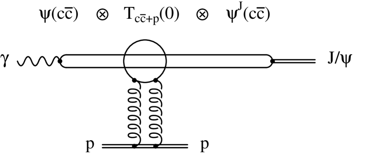
Figure 1: Schematic diagram for high energy diffractive $J/\psi$ photoproduction. The factorized form follows since, in the proton rest frame, the scattering of the $c\overline{c}$ system occurs over a much shorter timescale than the $\gamma\rightarrow c\overline{c}$ fluctuation or the $J/\psi$ formation times.

To lowest-order the $\gamma^{*}p\rightarrow J/\psi p$ amplitude can be factorized into the product of the $\gamma\rightarrow c\overline{c}$ transition, followed by the scattering of the $c\overline{c}$ system on the proton via (colourless) two-gluon exchange, and finally the formation of the $J/\psi$ from the outgoing $c\overline{c}$ pair. The sequence is sketched in Fig. 1. The crucial observation is that at high energy the scattering on the proton occurs over a much shorter timescale than the $\gamma\rightarrow c\overline{c}$ fluctuation or the $J/\psi$ formation times. Moreover the two-gluon exchange amplitude can be shown to be directly proportional to the gluon density $g(x,\overline{Q}^{2})$ with

$$x\;=\;(M_{\psi}^{2}+Q^{2})/W^{2},\;\;\;\;\;\overline{Q}^{2}\;=\;\textstyle{\frac{1}{4}}\>(M_{\psi}^{2}+Q^{2}).$$ (1)

In view of the importance of this connection, the corrections to the leading-order formula [2, 3] have been studied [4, 5]. It turns out that the major ambiguity is associated with the $J/\psi$ wave function. In particular there are sizeable normalization uncertainties which arise from allowing for the relativistic motion of the $c$ and $\overline{c}$ quarks within the $J/\psi$ meson. Even though the normalization is not precisely determined, it is advocated [4] that the “shape” (or $W$ dependence) of the cross section for $J/\psi$ diffractive production at high energies can serve as a valuable probe of the small $x$ behaviour of the gluon.

From a theoretical point of view the study of diffractive open charm production has some advantages as compared to $J/\psi$ production. It avoids the ambiguities associated with the $J/\psi$ wave function and yet retains the quadratic sensitivity to the gluon distribution. Moreover, in contrast to $J/\psi$, for open charm we can study the QCD behaviour as a function of $M$, the invariant mass of the $c\overline{c}$ system. In principle due to the heavy quark mass, perturbative QCD can predict both the cross sections $\sigma^{L,T}$ for diffractive $c\overline{c}$ production from longitudinally and transversely polarised photons. Indeed we find this to be the case. We compute both the $Q^{2}$ and $M^{2}$ dependence of $\sigma_{T}$ and $\sigma_{L}$ by integrating over the transverse momenta $(k_{T})$ of the produced $c$ and $\overline{c}$ quarks, and over the transverse momenta $(\ell_{T})$ of the exchanged gluons. Another feature is that the relevant scale at which the gluon is sampled in the diffractive production of open charm is

$$(m_{c}^{2}\>+\>k_{T}^{2})\;\left(1\>+\>\frac{Q^{2}}{M^{2}}\right),$$ (2)

which grows with $Q^{2}$. Besides (lowest-order) $c\overline{c}$ production we estimate higher-order QCD corrections arising from real and virtual gluon emissions. Recall that in the Drell-Yan process the ${\cal O}(\alpha_{S})$ contributions contain $\pi^{2}$ factors and that on resummation of these terms we obtain a significant enhancement of the cross section. In section 3 we will show that the ${\cal O}(\alpha_{S})$ correction to diffractive $c\overline{c}$ production also has a $\pi^{2}$ enhancement.

2. The basic formulae for diffractive open charm production

Here we study the diffractive production of a $c\overline{c}$ pair of invariant mass $M$ from a photon of virtuality $Q^{2}$ at high $\gamma p$ c.m. energy $\sqrt{s}$. The lowest order diagram for the process $\gamma^{*}p\rightarrow c\overline{c}p$ is shown in Fig. 2. The Bjorken $x$ variable is given by

$$x_{B}\;=\;Q^{2}/s.$$ (3)

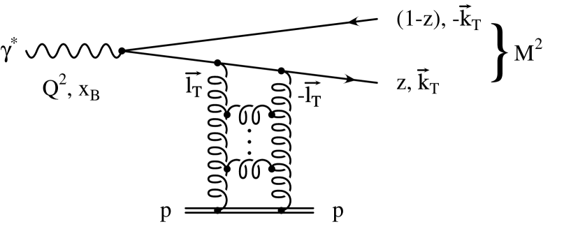
Figure 2: Diffractive open charm production in high energy $\gamma^{*}p$ collisions, where $z$ is the fraction of the energy of the photon that is carried by the charm quark.

As usual for a high energy diffractive process we introduce the variables

$$x_{{I\!\!P}}\;=\;\frac{Q^{2}\>+\>M^{2}}{s},$$ (4)

which is the longitudinal fraction of the proton energy carried by the “Pomeron” represented by the two-gluon exchange ladder in Fig. 2, and

$$\beta\;=\;\frac{Q^{2}}{Q^{2}\>+\>M^{2}}\;=\;\frac{x_{B}}{x_{{I\!\!P}}}.$$ (5)

The transverse momenta of the outgoing $c$ and $\overline{c}$ quarks are denoted by $\pm\mbox{\boldmath$k$}_{T}$, and those of the exchanged gluons by $\pm\mbox{\boldmath$\ell$}_{T}$; we are studying near-forward production.

It is convenient to use light-cone perturbation theory (see, for example, ref. [6]) and to express the particle four momenta in the form

$$k_{\mu}\;=\;(k_{+},k_{-},\mbox{\boldmath$k$}_{T})$$ (6)

where $k_{\pm}=k_{0}\pm k_{3}$. In this approach all the particles are on mass-shell, $k^{2}=k_{+}k_{-}-\mbox{\boldmath$k$}_{T}^{2}=m^{2}$, and $k_{+}$ and $\mbox{\boldmath$k$}_{T}$ are conserved at each vertex. We choose to work in a frame in which the target proton is essentially at rest and where the other particles are fast with four momenta

$$q_{\mu} = (q_{+},\;-Q^{2}/q_{+},\;{\bf 0}),$$

$$k_{\mu} = (k_{+},\;m_{T}^{2}/k_{+},\;\mbox{\boldmath$k$}_{T}),$$ (7)

$$\ell_{\mu} = (\ell_{+},\;\mbox{\boldmath$\ell$}_{T}^{2}/\ell_{+},\;\mbox{\boldmath$\ell$}_{T}),$$

with

$$m_{T}^{2}\equiv m^{2}+\mbox{\boldmath$k$}_{T}^{2},$$

where $m$ is the mass of the charm quark.

2.1. Factorization of the diffractive $\gamma^{*}\rightarrow c\overline{c}$ cross section

The differential cross section for the diffractive production of a $c\overline{c}$ pair of invariant mass $M$ is

$$\left.\frac{d^{2}\sigma}{dM^{2}dt}\right|_{t=0}\;=\;\sum_{\lambda,\lambda^{\prime}}\>\int\>\frac{d^{2}k_{T}dz}{16\pi^{3}}\;\delta\left(M^{2}\>-\>\frac{m_{T}^{2}}{z(1-z)}\right)\;\frac{1}{16\pi s^{2}}\>\left|{\cal M}_{\lambda\lambda^{\prime}}\right|^{2}$$ (8)

where ${\cal M}_{\lambda\lambda^{\prime}}$ is the amplitude for the production of a $c$ and $\overline{c}$ (with helicities $\lambda$ and $\lambda^{\prime}$) from the virtual photon. The $\delta$-function arises because the mass $M$ system is formed by $c$ and $\overline{c}$ quarks with $k_{+}$ components $zq_{+}$ and $(1-z)q_{+}$. We may rewrite (8) in the form

$$x_{{I\!\!P}}\>\left.\frac{d^{2}\sigma}{dx_{{I\!\!P}}dt}\right|_{0}\;=\;\sum_{\lambda,\lambda^{\prime}}\>\frac{M^{2}+Q^{2}}{M^{2}}\>\int\>\frac{d^{2}k_{T}dz}{16\pi^{3}}\>\frac{m_{T}^{2}}{M^{2}}\;\delta\left(z(1-z)\>-\>\frac{m_{T}^{2}}{M^{2}}\right)\>\frac{1}{16\pi s^{2}}\;\left|{\cal M}_{\lambda\lambda^{\prime}}\right|^{2}.$$ (9)

As mentioned in the introduction, the high-energy diffractive $c\overline{c}$ production amplitude ${\cal M}_{\lambda\lambda^{\prime}}$ can be factorized into the light-cone wave function $\psi_{\lambda\lambda^{\prime}}$ of the $c\overline{c}$ pair in the virtual photon and the (helicity-conserving) amplitude $T_{\lambda\lambda^{\prime}}$ for the scattering of the $c\overline{c}$ pair on the target proton. In analogy to ref. [3] we have

$${\cal M}_{\lambda\lambda^{\prime}}(k_{T},z)\;=\;\sqrt{N_{C}}\>\int\>d^{2}k_{T}^{\prime}\>\int_{0}^{1}\>dz^{\prime}\>\psi_{\lambda\lambda^{\prime}}(k_{T}^{\prime},z^{\prime})\>T_{\lambda\lambda^{\prime}}(k_{T}^{\prime},z^{\prime};k_{T},z),$$ (10)

where $\sqrt{N_{C}}$ occurs in the amplitude, since the cross section is the sum over the number of colours $N_{C}=3$ of the charm quark.

The factorization of ${\cal M}$ follows since the lifetime $\tau_{\gamma}$ of the $c\overline{c}$ fluctuation of the virtual photon is much longer than the time of interaction with the gluons $\tau_{i}$. It is informative to recall the argument of why this is so. According to the uncertainty principle the fluctuation time

$$\tau_{\gamma}\>\sim\>\frac{1}{\Delta E}\;=\;\left|\frac{1}{q_{-}-k_{1-}-k_{2-}}\right|\;=\;\frac{z(1-z)q_{+}}{\overline{Q}^{2}+k_{T}^{2}}$$ (11)

where $k_{1}$ and $k_{2}$ are the four momenta of the quarks of mass $m$, and

$$\overline{Q}^{2}\;\equiv\;z(1-z)Q^{2}\>+\>m^{2}.$$ (12)

An estimate of the interaction time can be obtained from the typical time for the emission of a gluon with momentum $\ell$, from the quark $k_{1}$, say. Then

$$\tau_{i}\>\sim\>\left|\frac{1}{k_{1-}-k_{1-}^{\prime}-\ell_{-}}\right|\;=\;\left|\frac{q_{+}}{m_{T}^{2}/z-m_{T}^{2}/z^{\prime}-\ell_{T}^{2}/\alpha}\right|$$ (13)

where $\alpha=\ell_{+}/q_{+}$ and $z^{\prime}=z-\alpha$. In the leading $\log 1/x$ approximation we have $\alpha\ll z$ and hence

$$\tau_{i}\;\approx\;\frac{\alpha q_{+}}{\ell_{T}^{2}}\;\ll\;\tau_{\gamma}.$$ (14)

At high $Q^{2}$ the argument becomes particularly transparent. Then from (11) we have

$$\tau_{\gamma}\>\sim\>\frac{q_{+}}{Q^{2}}\;=\;\frac{1}{m_{p}x_{B}},$$ (15)

whereas (14) gives

$$\tau_{i}\>\sim\>\frac{\ell_{+}}{\ell_{T}^{2}}\;=\;\frac{1}{m_{p}x_{\ell}}$$ (16)

where $x_{\ell}$ is the Bjorken variable for the gluon-proton interaction and $m_{p}$ is the mass of the proton. We are concerned with the kinematic region $x_{B}\ll x_{\ell}$ where the leading $\log(x_{\ell}/x_{B})$ approximation is appropriate, and so we have $\tau_{\gamma}\gg\tau_{i}$.

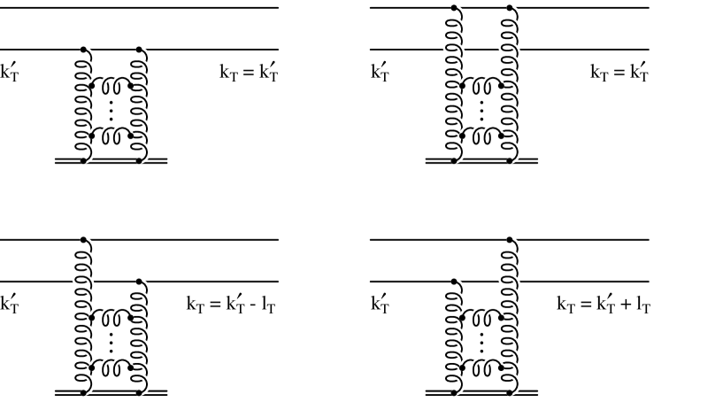
Figure 3: Graphs which contribute to the amplitude $T_{\lambda^{\prime}\lambda}(k_{T}^{\prime},z^{\prime};k_{T},z)$ for the scattering of the $c\overline{c}$ pair off the target proton. At high energy $z=z^{\prime}$ and the quark helicities ($\lambda$ and $\lambda^{\prime}$) are conserved.

During the short interaction time $\tau_{i}$ the exchanged gluons change only the quark (and/or antiquark) transverse momenta, and leave their energy fractions and helicities unchanged. Thus $T_{\lambda\lambda^{\prime}}$ can be simply computed as the sum of the light-cone perturbation theory graphs shown in Fig. 3. We have [3]

$$T_{\lambda\lambda^{\prime}}(k_{T}^{\prime},k_{T})\;=\;i\>\frac{4\pi s}{2N_{C}}\>\int\>\frac{d^{2}\ell_{T}}{\ell_{T}^{4}}\;\biggl{[}2\delta(\mbox{\boldmath$k$}_{T}^{\prime}-\mbox{\boldmath$k$}_{T})\>-\>\delta(\mbox{\boldmath$k$}_{T}^{\prime}-\mbox{\boldmath$k$}_{T}-\mbox{\boldmath$\ell$}_{T})\>-\>\delta(\mbox{\boldmath$k$}_{T}^{\prime}-\mbox{\boldmath$k$}_{T}+\mbox{\boldmath$\ell$}_{T})\biggr{]}\;\alpha_{S}(\ell_{T}^{2})\>f(x_{I\!\!P},\ell_{T}^{2}),$$ (17)

where in the leading $\ln(1/x)$ approximation, $z=z^{\prime}$ and $T_{\lambda\lambda^{\prime}}$ becomes independent of $z$ and $z^{\prime}$. The factor $1/\ell_{T}^{4}$ arises from the propagators of the two exchanged gluons. The factor $1/2N_{C}$ arises from the colour coupling of the gluon to the quark and the $4\pi$ from the usual coupling relation $g_{s}^{2}=4\pi\alpha_{S}$. The factor $s$ arises since our amplitude $T$ is defined so that the optical theorem reads “Im $T=s\sigma$”. The distribution $f(x_{I\!\!P},\ell_{T}^{2})$ is the probability of finding a $t$-channel gluon with transverse momentum $\ell_{T}$. That is $f$ is the gluon density unintegrated over $\ell_{T}^{2}$ or, to be precise, $\ln\ell_{T}^{2}$. It satisfies the BFKL equation, which effectively resums the leading $\alpha_{S}\ln(1/x)$ contributions. We have tacitly assumed that we are considering a forward “elastic” scattering amplitude with $t=0$. However, the minimum value of $|t|$ is

$$t_{min}\;=\;\left(\frac{Q^{2}+M^{2}}{W^{2}}\>m_{p}\right)^{2}\;\approx\;x_{I\!\!P}^{2}m_{p}^{2}.$$ (18)

The $t_{min}$ effects are expected to be small even up to $x_{I\!\!P}$ of about 0.1 [4]. To relate $f$ to the conventional gluon density, which satisfies GLAP evolution, we must integrate over $\ell_{T}^{2}$. We have

$$x_{I\!\!P}g(x_{I\!\!P},Q^{2})\;=\;\int^{Q^{2}}\>\frac{d\ell_{T}^{2}}{\ell_{T}^{2}}\>f(x_{I\!\!P},\ell_{T}^{2})$$ (19)

and the inverse relation

$$f(x_{I\!\!P},\ell_{T}^{2})\;=\;\ell_{T}^{2}\>\frac{\partial(x_{I\!\!P}g(x_{I\!\!P},\ell_{T}^{2}))}{\partial\ell_{T}^{2}}.$$ (20)

On substituting (17) into (10) we have

$${\cal M}_{\lambda\lambda^{\prime}}\;=\;i\>\frac{4\pi^{2}s}{2\sqrt{N_{C}}}\>\int\>\frac{d\ell_{T}^{2}}{\ell_{T}^{4}}\;\Delta\psi_{\lambda\lambda^{\prime}}\>\alpha_{S}(\ell_{T}^{2})\>f(x_{I\!\!P},\ell_{T}^{2}),$$ (21)

where $\Delta\psi$ is the combination

$$\Delta\psi(\mbox{\boldmath$k$}_{T},\mbox{\boldmath$\ell$}_{T},z)\;=\;2\psi(\mbox{\boldmath$k$}_{T},z)\>-\>\psi(\mbox{\boldmath$k$}_{T}-\mbox{\boldmath$\ell$}_{T},z)\>-\>\psi(\mbox{\boldmath$k$}_{T}+\mbox{\boldmath$\ell$}_{T},z).$$ (22)

To evaluate $\Delta\psi$ of (22) we need the photon wave function [3, 7, 8]. We use the convention of ref. [6] and express it in the form

$$\psi_{\lambda\lambda^{\prime}}(k_{T},z)\;=\;-ee_{c}\>\sqrt{z(1-z)}\;\frac{\overline{u}_{\lambda}(k_{T},z)\>\gamma\cdot\epsilon\>v_{\lambda^{\prime}}(-k_{T},1-z)}{\overline{Q}^{2}+k_{T}^{2}}$$ (23)

where $ee_{c}=\frac{2}{3}e$ is the charge of the charm quark, $\epsilon$ is the polarisation vector of the photon, and $\overline{Q}^{2}$ is given by (12).

2.2. The helicity amplitudes for diffractive $c\overline{c}$ production

In this subsection we explicitly evaluate the helicity amplitudes ${\cal M}_{\lambda\lambda^{\prime}}^{\lambda(\gamma)}$ which describe the diffractive production of a $c\overline{c}$ pair with helicities $\lambda,\lambda^{\prime}$ from a photon of helicity $\lambda(\gamma)$. First we obtain the amplitudes for production from a longitudinally polarised photon and then from a transversely polarised photon.

The four momentum of the photon has the form $q_{\mu}=(q_{+},\>-Q^{2}/q_{+},\>{\bf 0})$, see (S0.Ex1), and thus a longitudinally polarised photon is described by the polarisation vector

$$\epsilon_{L}\;=\;(q_{+}/Q,\>Q/q_{+},{\bf 0}).$$ (24)

In order to evaluate (23) with $\epsilon=\epsilon_{L}$ we first note that

$$q^{\mu}\overline{u}_{\lambda}\gamma_{\mu}v_{\lambda^{\prime}}\;=\;\frac{1}{2}\>(q_{+}\overline{u}_{\lambda}\gamma_{-}v_{\lambda^{\prime}}\;+\;q_{-}\overline{u}_{\lambda}\gamma_{+}v_{\lambda^{\prime}})\;=\;0$$

so that we have

$$\overline{u}\gamma_{-}v\;=\;\frac{Q^{2}}{q_{+}^{2}}\>\overline{u}\gamma_{+}v.$$ (25)

We may use this identity to evaluate the matrix element which occurs in (23)

$$\overline{u}_{\lambda}\>\gamma.\epsilon\>v_{\lambda^{\prime}} = \frac{1}{2}\>\left(\frac{q_{+}}{Q}\>\overline{u}_{\lambda}\gamma_{-}v_{\lambda^{\prime}}\>+\>\frac{Q}{q_{+}}\>\overline{u}_{\lambda}\gamma_{+}v_{\lambda^{\prime}}\right)\;=\;\frac{Q}{q_{+}}\>\overline{u}_{\lambda}\gamma_{+}v_{\lambda^{\prime}}$$ (26)

$$= 2\>Q\>\sqrt{z(1-z)}\>\delta_{\lambda,-\lambda^{\prime}}$$

see, for example, ref. [6]. Using (23) and (26) we can evaluate $\Delta\psi$ for longitudinally polarised photons. We obtain

$$\Delta\psi_{\lambda\lambda^{\prime}}^{L}\;=\;-2\delta_{\lambda,-\lambda^{\prime}}\>ee_{c}\>Q\>z(1-z)\;\left[\frac{2}{\overline{Q}^{2}+k_{T}^{2}}\>-\>\frac{1}{\overline{Q}^{2}+(\mbox{\boldmath$k$}_{T}-\mbox{\boldmath$\ell$}_{T})^{2}}\>-\>\frac{1}{\overline{Q}^{2}+(\mbox{\boldmath$k$}_{T}+\mbox{\boldmath$\ell$}_{T})^{2}}\right].$$ (27)

We substitute $\Delta\psi^{L}$ in (21) and carry out the angular integration. We find the amplitudes for the production of $c$ and $\overline{c}$ quarks with helicities $\lambda,\lambda^{\prime}$ from a longitudinally polarised photon to be

$${\cal M}_{\lambda\lambda^{\prime}}^{L}\;=\;-4\delta_{\lambda,-\lambda^{\prime}}\>ee_{c}\>Q\>z(1-z)\;\left(i\>\frac{2\pi^{2}s}{\sqrt{N_{C}}}\right)\>{\cal I}_{1}(k_{T}^{2})$$ (28)

where the integral over the transverse momenta of the exchanged gluons is

$${\cal I}_{1}(k_{T}^{2})\;=\;\int\>\frac{d\ell_{T}^{2}}{\ell_{T}^{4}}\>\alpha_{S}(\ell_{T}^{2})\>f(x_{I\!\!P},\ell_{T}^{2})\>\left(\frac{1}{\overline{Q}^{2}+k_{T}^{2}}\>-\>\frac{1}{Q_{k\ell}^{2}}\right).$$ (29)

Here we have introduced

$$Q_{k\ell}^{2}\;=\;\sqrt{(\overline{Q}^{2}+k_{T}^{2}+\ell_{T}^{2})^{2}\>-\>4k_{T}^{2}\ell_{T}^{2}}.$$ (30)

In order to calculate the helicity amplitudes for diffractive $c\overline{c}$ production from a transversely polarised incoming photon it is convenient to evaluate [7, 6] the matrix element $\overline{u}\mbox{\boldmath$\gamma$}_{T}\cdot\mbox{\boldmath$\epsilon$}_{T}v$ using as a basis the circular polarisation vectors of the photon

$$\epsilon_{\pm}\;=\;\frac{1}{\sqrt{2}}\>(0,0,1,\pm i).$$ (31)

Then we obtain

$$\overline{u}_{\lambda}(\mbox{\boldmath$\gamma$}_{T}.\mbox{\boldmath$\epsilon$}_{\pm})v_{\lambda^{\prime}}\;=\;\frac{1}{\sqrt{z(1-z)}}\>\biggl{(}\delta_{\lambda,-\lambda^{\prime}}\left\{(1-2z)\lambda\>\overline{+}1\right\}\>\mbox{\boldmath$\epsilon$}_{\pm}\cdot\mbox{\boldmath$k$}_{T}\>+\>\delta_{\lambda\lambda^{\prime}}\>m\lambda\biggr{)},$$ (32)

where here quark helicities of $\pm\frac{1}{2}$ are represented by $\lambda=\pm 1$. In this polarisation basis we have

$$\Delta\psi_{\lambda\lambda^{\prime}}^{\pm} = -ee_{c}\>\delta_{\lambda,-\lambda^{\prime}}\left\{(1-2z)\lambda\overline{+}1\right\}\;\left[\frac{2\mbox{\boldmath$\epsilon$}_{\pm}\cdot\mbox{\boldmath$k$}_{T}}{\overline{Q}^{2}+k_{T}^{2}}\>-\>\frac{\mbox{\boldmath$\epsilon$}_{\pm}\cdot(\mbox{\boldmath$k$}_{T}-\mbox{\boldmath$\ell$}_{T})}{\overline{Q}^{2}+(\mbox{\boldmath$k$}_{T}-\mbox{\boldmath$\ell$}_{T})^{2}}\>-\>\frac{\mbox{\boldmath$\epsilon$}_{\pm}\cdot(\mbox{\boldmath$k$}_{T}+\mbox{\boldmath$\ell$}_{T})}{\overline{Q}^{2}+(\mbox{\boldmath$k$}_{T}+\mbox{\boldmath$\ell$}_{T})^{2}}\right]$$ (33)

$$-ee_{c}\>\delta_{\lambda\lambda^{\prime}}\>m\lambda\;\left[\frac{2}{\overline{Q}^{2}+k_{T}^{2}}\>-\>\frac{1}{\overline{Q}^{2}+(\mbox{\boldmath$k$}_{T}-\mbox{\boldmath$\ell$}_{T})^{2}}\>-\>\frac{1}{\overline{Q}^{2}+(\mbox{\boldmath$k$}_{T}+\mbox{\boldmath$\ell$}_{T})^{2}}\right].$$

As before we substitute $\Delta\psi^{\pm}$ into (21) and carry out the angular integration. We obtain the helicity amplitudes

$${\cal M}_{\lambda\lambda^{\prime}}^{\pm}\;=\;-2ee_{c}\>\left(i\>\frac{2\pi^{2}s}{\sqrt{N_{C}}}\right)\>\biggl{(}\delta_{\lambda,-\lambda^{\prime}}\left\{(1-2z)\lambda\overline{+}1\right\}\>\mbox{\boldmath$\varepsilon$}_{\pm}.\mbox{\boldmath$k$}_{T}\>{\cal I}_{2}(k_{T}^{2})\>+\>\delta_{\lambda\lambda^{\prime}}m\lambda\>{\cal I}_{1}(k_{T}^{2})\biggr{)}$$ (34)

where the integral ${\cal I}_{1}$ is given by (29) and

$${\cal I}_{2}(k_{T}^{2})\;=\;\int\>\frac{d\ell_{T}^{2}}{\ell_{T}^{4}}\>\alpha_{S}(\ell_{T}^{2})\>f(x_{I\!\!P},\ell_{T}^{2})\;\left(\frac{1}{\overline{Q}^{2}+k_{T}^{2}}\>-\>\frac{1}{2k_{T}^{2}}\>+\>\frac{\overline{Q}^{2}-k_{T}^{2}+\ell_{T}^{2}}{2k_{T}^{2}Q_{k\ell}^{2}}\right)$$ (35)

with $\overline{Q}^{2}$ and $Q_{k\ell}^{2}$ defined as in (12) and (30) respectively.

Asymptotically, when $\overline{Q}^{2}+k_{T}^{2}\gg\ell_{T}^{2}$, the $\ell_{T}^{2}$ integration gives a logarithmic contribution of the form $\ln[(\overline{Q}^{2}+k_{T}^{2})/\mu^{2}]$, or rather like $1/\gamma$ if the anomalous dimension $\gamma$ of the gluon distribution is taken into account. At realistic energies non-logarithmic contributions are appreciable and the integrations ${\cal I}_{1,2}(k_{T}^{2})$ have to be performed explicitly. The important domain of integration is $\mu^{2}\lower 3.01385pt\hbox{$\;\stackrel{{\scriptstyle\textstyle<}}{{\sim}}\;$}\ell_{T}^{2}\lower 3.01385pt\hbox{$\;\stackrel{{\scriptstyle\textstyle<}}{{\sim}}\;$}\overline{Q}^{2}+k_{T}^{2}$.

2.3. The diffractive $\gamma_{T,L}\rightarrow c\overline{c}$ cross sections

To evaluate the cross sections for open charm production we need to sum $|{\cal M}|^{2}$ over the quark helicities $\lambda$ and $\lambda^{\prime}$. For production from longitudinally polarised photons we have from (28)

$$\sum_{\lambda,\lambda^{\prime}}\left|{\cal M}_{\lambda\lambda^{\prime}}^{L}\right|^{2}\;=\;\frac{4\pi^{4}s^{2}}{3}\>32\>e^{2}e_{c}^{2}\>z^{2}(1-z)^{2}\>Q^{2}\>|{\cal I}_{1}|^{2},$$ (36)

while for transversely polarised photons we must average over the two transverse polarisation states $\lambda(\gamma)=\pm$. From (34) we have

$$\frac{1}{2}\>\sum_{\lambda(\gamma)=\pm}\>\sum_{\lambda,\lambda^{\prime}}\>\left|{\cal M}_{\lambda,\lambda^{\prime}}^{\lambda(\gamma)}\right|^{2}\;=\;\frac{4\pi^{4}s^{2}}{3}\>8e^{2}e_{c}^{2}\>\biggl{(}k_{T}^{2}\{z^{2}+(1-z)^{2}\}\>|{\cal I}_{2}|^{2}\>+\>m^{2}\>|{\cal I}_{1}|^{2}\biggr{)}.$$ (37)

We are now ready to calculate the cross sections from (9). On carrying out the $z$ integration in (9) we find that the $\delta$ function gives a Jacobian factor $2(1-4m_{T}^{2}/M^{2})^{-\frac{1}{2}}$, and moreover implies that

$$z(1-z) = \frac{m_{T}^{2}}{M^{2}},$$

$$z^{2}\>+\>(1-z)^{2} = 1\>-\>\frac{2m_{T}^{2}}{M^{2}}\;=\;1\>-\>\frac{2\beta}{1-\beta}\>\frac{m_{T}^{2}}{Q^{2}}\;\equiv\;1\>-\>\frac{2\beta K^{2}}{Q^{2}},$$

where we have defined

$$K^{2}\;\equiv\;\frac{m^{2}+k_{T}^{2}}{1-\beta}.$$ (38)

The variable $K^{2}$ turns out to be the scale probed by the process, since after the $z$ integration

$$\overline{Q}^{2}\>+\>k_{T}^{2}\;=\;Q^{2}\>\frac{m_{T}^{2}}{M^{2}}\>+\>m_{T}^{2}\;=\;\frac{m_{T}^{2}}{1-\beta}\;\equiv\;K^{2}.$$ (39)

Collecting the factors together and inserting into (9) we find that the cross section for diffractive open charm production from longitudinally polarised photons is

$$x_{{I\!\!P}}\>\left.\frac{d^{2}\sigma^{L}}{dx_{{I\!\!P}}dt}\right|_{0}\;=\;\frac{4\pi^{2}e_{c}^{2}\alpha}{3}\;\frac{Q^{2}}{1-\beta}\>\int_{0}^{\frac{1}{4}M^{2}-m^{2}}\frac{dk_{T}^{2}}{\sqrt{1-4m_{T}^{2}/M^{2}}}\>\left(\frac{m_{T}^{2}}{M^{2}}\right)^{3}\>|{\cal I}_{1}|^{2},$$ (40)

and from transversely polarised photons is

$$x_{{I\!\!P}}\>\left.\frac{d^{2}\sigma^{T}}{dx_{{I\!\!P}}dt}\right|_{0}\;=\;\frac{\pi^{2}e_{c}^{2}\alpha}{3(1-\beta)}\>\int_{0}^{\frac{1}{4}M^{2}-m^{2}}\>\frac{dk_{T}^{2}}{\sqrt{1-4m_{T}^{2}/M^{2}}}\>\frac{m_{T}^{2}}{M^{2}}\>\left(k_{T}^{2}\>\left(1-\frac{2\beta K^{2}}{Q^{2}}\right)\>|{\cal I}_{2}|^{2}\>+\>m^{2}|{\cal I}_{1}|^{2}\right)$$ (41)

where recall that $m_{T}^{2}\equiv m^{2}+k_{T}^{2}$ and $\beta=Q^{2}/(Q^{2}+M^{2})$. The masses $m$ and $M$ are those of the $c$ quark and the $c\overline{c}$ system respectively, and $\alpha$ is the electromagnetic coupling.

2.4. Leading logarithmic approximation

In practice the ${\cal I}_{1,2}$ integrations over $\ell_{T}^{2}$ of (29) and (35) have to be performed explicitly, with the main contribution arising from the domain $\ell_{T}^{2}\lower 3.01385pt\hbox{$\;\stackrel{{\scriptstyle\textstyle<}}{{\sim}}\;$}\overline{Q}^{2}+k_{T}^{2}$. However, before we do this, it is informative to derive analytical expressions for the integrals assuming that the main contribution comes from the region $\ell_{T}^{2}\ll\overline{Q}^{2}+k_{T}^{2}$. That is we expand the terms in brackets in (29) and (35) in the form $c_{1}\ell_{T}^{2}+c_{2}\ell_{T}^{4}+\ldots$ and retain only the $c_{1}$ term. In this approximation ${\cal I}_{1,2}$ are given by

$${\cal I}_{1}^{LLA}(k_{T}^{2}) = \frac{\overline{Q}^{2}-k_{T}^{2}}{(\overline{Q}^{2}+k_{T}^{2})^{3}}\>\alpha_{S}(\overline{Q}^{2}+k_{T}^{2})\>x_{I\!\!P}g(x_{I\!\!P},\overline{Q}^{2}+k_{T}^{2}),$$ (42)

$${\cal I}_{2}^{LLA}(k_{T}^{2}) = \frac{2\overline{Q}^{2}}{(\overline{Q}^{2}+k_{T}^{2})^{3}}\>\alpha_{S}(\overline{Q}^{2}+k_{T}^{2})\>x_{I\!\!P}g(x_{I\!\!P},\overline{Q}^{2}+k_{T}^{2})$$ (43)

where we have used (19) to express the answer in terms of the conventional gluon distribution.

If we use these results to evaluate $|{\cal M}|^{2}$ and substitute them into (9) then we find, in this approximation, that the cross sections are given by

$$x_{{I\!\!P}}\>\left.\frac{d^{2}\sigma^{L}}{dx_{{I\!\!P}}dt}\right|_{0}\;=$$

$$\;\;\;\;\;\frac{4\pi^{2}e_{c}^{2}\alpha}{3Q^{4}}\;\beta^{3}\>\int_{0}^{\frac{1}{4}M^{2}-m^{2}}\frac{dk_{T}^{2}}{\sqrt{1-4m_{T}^{2}/M^{2}}}\>\frac{[m_{T}^{2}-2(1-\beta)k_{T}^{2}]^{2}}{(m_{T}^{2})^{3}}\biggl{(}\alpha_{S}(K^{2})\>x_{{I\!\!P}}g(x_{{I\!\!P}},K^{2})\biggr{)}^{2},$$

(44)

$$x_{{I\!\!P}}\>\left.\frac{d^{2}\sigma^{T}}{dx_{{I\!\!P}}dt}\right|_{0}\;=\;\frac{4\pi^{2}e_{c}^{2}\alpha}{3Q^{2}}\>\beta(1-\beta)^{2}\>\int_{0}^{\frac{1}{4}M^{2}-m^{2}}\>\frac{dk_{T}^{2}}{\sqrt{1-4m_{T}^{2}/M^{2}}}$$

$$\left\{\frac{k_{T}^{2}(m^{2}+\beta k_{T}^{2})^{2}\>(1-2\beta K^{2}/Q^{2})}{(m_{T}^{2})^{5}}\>+\>\frac{m^{2}}{4}\>\frac{[m_{T}^{2}-2(1-\beta)k_{T}^{2}]^{2}}{(m_{T}^{2})^{5}}\right\}\;\biggl{(}\alpha_{S}(K^{2})\>x_{{I\!\!P}}g(x_{{I\!\!P}},K^{2})\biggr{)}^{2},$$

where the scale $K^{2}$ is given by (38).

The scale $K^{2}$ for diffractive processes has been emphasized by Bartels et al. [9] and by Genovese et al. [10]. Ref. [9] concerns light quark-antiquark production and the “hardness” of the scale $K^{2}$, and the validity of perturbative QCD is ensured by considering quark jets at large $k_{T}^{2}$. Ref. [10] discusses open charm production, based on earlier work starting from ref. [11]. It contains similar cross section formulae to (40) and (41), together with the logarithmic approximations of the form of (S0.Ex13) and (S0.Ex18). In particular the hardness of the scale $K^{2}=(m^{2}+k_{T}^{2})/(1-\beta)$ is emphasized, although the numerical predictions are made using the leading logarithmic approximation only, with the scale $K^{2}$ set equal to $m^{2}$. Here, in section 4, we extend the numerical treatment to calculate explicitly the integrals ${\cal I}_{1,2}$ over the exchanged gluon transverse momenta $\ell_{T}$, and moreover we evaluate the higher order contributions (of section 3). We shall see that the predicted values of the cross sections for diffractive $c\overline{c}$ production are considerably enhanced by both of these effects.

2.5. Connection with diffractive $J/\psi$ production

It is instructive to see how these approximate cross section formulae given in (S0.Ex13) and (S0.Ex18) compare with the result which was derived for the exclusive production of heavy quark-antiquark mesons [2-4]. A convenient way to make the comparison is to consider the production of the mesonic states with $M^{2}=M_{V}^{2}\ll\tilde{Q}^{2}$ where

$$\tilde{Q}^{2}\;\equiv\;Q^{2}\>+\>M_{V}^{2}.$$ (46)

The kinematic region for such a reaction corresponds to

$$\beta\;=\;1\>-\>\frac{M_{V}^{2}}{\tilde{Q}^{2}}\;\rightarrow\;1$$ (47)

at large $\tilde{Q}^{2}/M_{V}^{2}$. In this kinematic region we can rewrite the cross section formulae (S0.Ex13) and (S0.Ex18) in the form

$$M^{2}\left.\frac{d^{2}\sigma^{L}}{dM^{2}dt}\right|_{0} = (1-\beta)\>x_{{I\!\!P}}\>\left.\frac{d^{2}\sigma^{L}}{dx_{{I\!\!P}}dt}\right|_{0}$$ (48)

$$= \frac{4\pi^{2}e_{c}^{2}\alpha}{3}\;\frac{M_{V}^{2}Q^{2}}{\tilde{Q}^{8}}\>\int_{0}^{\frac{1}{4}M^{2}-m^{2}}\frac{dk_{T}^{2}}{\sqrt{1-4m_{T}^{2}/M^{2}}}\;\frac{1}{m_{T}^{2}}\;\biggl{(}\alpha_{S}(K^{2})\>x_{{I\!\!P}}\>g(x_{{I\!\!P}},K^{2})\biggr{)}^{2}$$

$$\approx \frac{4\pi^{2}e_{c}^{2}\alpha}{3}\;\frac{M_{V}^{2}Q^{2}}{(Q^{2}+M_{V}^{2})^{4}}\;\biggl{(}\alpha_{S}(\overline{Q}^{2})\>x_{{I\!\!P}}\>g(x_{{I\!\!P}},\overline{Q}^{2})\biggr{)}^{2}\>{\cal I}_{L},$$

$$M^{2}\left.\frac{d^{2}\sigma^{T}}{dM^{2}dt}\right|_{0} = \frac{4\pi^{2}e_{c}^{2}\alpha}{3}\;\frac{M_{V}^{4}}{\tilde{Q}^{8}}\int_{0}^{\frac{1}{4}M^{2}-m^{2}}\frac{dk_{T}^{2}}{\sqrt{1-4m_{T}^{2}/M^{2}}}\;\frac{M_{V}^{2}(m^{2}+2k_{T}^{2})}{4(m_{T}^{2})^{3}}\;\biggl{(}\alpha_{S}(K^{2})\>x_{{I\!\!P}}g(x_{{I\!\!P}},K^{2})\biggr{)}^{2}$$ (49)

$$\approx \frac{4\pi^{2}e_{c}^{2}\alpha}{3}\;\frac{M_{V}^{4}}{(Q^{2}+M_{V}^{2})^{4}}\;\biggl{(}\alpha_{S}(\overline{Q}^{2})\>x_{{I\!\!P}}\>g(x_{{I\!\!P}},\overline{Q}^{2})\biggr{)}^{2}\>{\cal I}_{T}$$

where the scale $\overline{Q}^{2}$ is obtained by neglecting $k_{T}^{2}$ in $K^{2}$, that is $\overline{Q}^{2}\approx\frac{1}{4}(Q^{2}+M_{V}^{2})$, and where ${\cal I}_{L,T}$ denote the integrals over $k_{T}^{2}$. For the exclusive diffractive production of a meson of mass $M_{V}$ the integrals ${\cal I}_{L,T}$ should be replaced by the overlap integrals of the virtual photon wave function with light-cone wave function of the $c\overline{c}$ pair in the meson [2-4].

Formulae (48) and (49) have precisely the structure found for the exclusive diffractive production of a meson of mass $M_{V}$ (see, for example, the $J/\psi$ diffractive production cross section given in eq. (2) of ref. [4]), including the result

$$\sigma_{L}/\sigma_{T}\;\sim\;Q^{2}/M_{V}^{2}.$$ (50)

However, to obtain reliable estimates of $\sigma_{L,T}(J/\psi)$ we need to evaluate the overlap integrals which replace ${\cal I}_{L,T}$ in (48) and (49). We return now to the subject of this paper, namely the diffractive production of open charm.

3. Higher order contributions to diffractive $c\overline{c}$ production

So far we have considered only lowest-order diffractive $c\overline{c}$ production. In this section we evaluate higher-order QCD corrections to the cross sections.

3.1. Real gluon emission contributions

We wish to calculate the contributions in which the incoming photon produces a $c\overline{c}g$ three jet configuration. As before, the time during which the two gluon exchange interacts with the $c\overline{c}g$ system is much less than the lifetime of the $c\overline{c}g$ fluctuation of the photon. So we can write the amplitude in factorized form and consider just the coupling of the exchanged gluons to the $c\overline{c}g$ state.

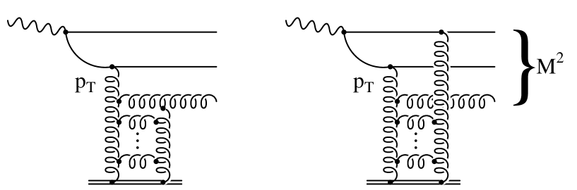
Figure 4: $c\overline{c}g$ contributions with strong ordering with the gluon having much smaller transverse momentum than the $c$ and $\overline{c}$.

We need to consider only diagrams with space-like evolution. Those with time-like evolution do not change the cross section apart from the corrections discussed in the next subsection. We divide the contributions according to the transverse momenta ordering of the $c,\overline{c}$ and $g$. First we have contributions when the transverse momentum of the final gluon is much less than that of the quarks. The two exchanged gluons can couple to any of the three outgoing partons. There are eighteen such diagrams, two of which are shown in Fig. 4. These diagrams initiate GLAP evolution of a diffractive state starting from a gluon of transverse momentum $p_{T}$. They give a $dM^{2}/M^{2}$ behaviour for $M^{2}\gg Q^{2},m^{2}$. In contrast in the kinematic region where the outgoing gluon has transverse momenta greater than one of the quarks we have a $dM^{2}/M^{4}$ behaviour. Fig. 5 shows such a contribution. It corresponds to GLAP evolution of a diffractive state starting from an initial quark (with transverse momentum $p_{T}$). Strictly speaking we should calculate the $c\overline{c}g$ contributions over all regions of phase space. At present the required formulae only exist for strong ordering of the transverse momenta. However, this should give a good estimate. In fact the situation is better than it first appears. For the low $M^{2}$ region lowest-order $c\overline{c}$ production is dominant. For higher $M^{2}$ we can use the so-called Pomeron-gluon splitting function, $P_{gP}$, which is given by [12]

$$P_{gP}(z)\;=\;\left(\frac{8N_{C}^{2}}{N_{C}^{2}-1}\right)\>\frac{1}{z}\>(1+2z)^{2}\>(1-z)^{3},$$ (51)

which is valid either for transverse-momentum ordering (with the outgoing gluon having the smallest transverse momentum) or in the BFKL limit of large $\ln(1/z)$. The latter corresponds to large $M^{2}$ where the $c\overline{c}g$ configuration becomes important.

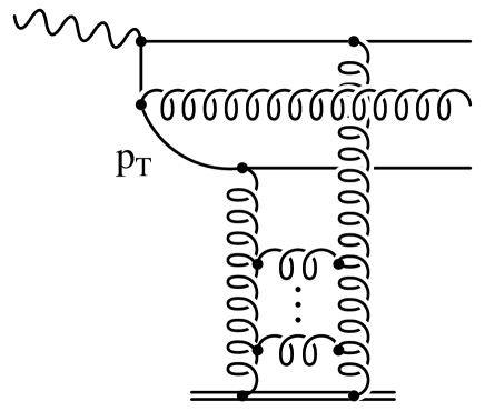
Figure 5: The $c\overline{c}g$ diagram driven by the quark distribution $(p_{T})$.

Using the formulae of ref. [12] with the coefficient functions of refs. [13, 14] we find

$$x_{{I\!\!P}}\>\left.\frac{d^{2}\sigma^{T,L}}{dx_{{I\!\!P}}dt}\right|_{0}\;=\;\frac{4\pi^{2}e_{c}^{2}\alpha}{Q^{2}}\>\frac{\alpha_{S}^{3}(\mu^{2})}{64\pi}\;2\beta\>\int_{z_{m}}^{1}\>\frac{dz}{z}\;C^{T,L}\left(\frac{\beta}{z},\>\frac{m^{2}}{Q^{2}}\right)\>P_{gP}(z)\>\int_{Q_{0}^{2}}^{\mu^{2}}\>\frac{dk_{T}^{2}}{k_{T}^{4}}\>\biggl{(}x_{{I\!\!P}}g(x_{{I\!\!P}},k_{T}^{2})\biggr{)}^{2}$$ (52)

where the lower limit $z_{m}$ is determined by the kinematical boundary

$$z_{m}\;=\;\beta\>\left(1\>+\>\frac{4m^{2}}{Q^{2}}\right)\;=\;\frac{Q^{2}+4m^{2}}{Q^{2}+M^{2}},$$ (53)

and the cut-off $Q_{0}^{2}$ is chosen to be 1 GeV². The leading-order coefficient functions are given by

$$C^{T}(x,r)\>+\>C^{L}(x,r) = \biggl{[}x^{2}\>+\>(1-x)^{2}\>+\>4x(1-3x)r\>-\>8x^{2}r^{2}\biggr{]}\;\ln\>\frac{1+v}{1-v}$$ (54)

$$+\;v\>\biggl{[}-1\>+\>8x(1-x)\>-\>4x(1-x)r\biggr{]},$$

$$C^{L}(x,r) = 4v\>x(1-x)\>-\>8x^{2}r\>\ln\>\frac{1+v}{1-v},$$ (55)

where $r=m^{2}/Q^{2}$ and $v$, the c.m. velocity of the $c$ quarks, is given by

$$v^{2}\;=\;1\>-\>\frac{4m^{2}x}{Q^{2}(1-x)}.$$ (56)

We take the mass factorization scale $\mu^{2}=4m^{2}$, since it was shown [15] that this is the most appropriate choice for the perturbative stability of (52).

From (54) and (55) we can gain insight into how gluon emission contributes to the evolution equation. For large $Q^{2}/m^{2}$ we can rewrite (54) and (55) in the form

$$C^{T}(x,r) = [x^{2}+(1-x)^{2}]\>\ln\>\frac{Q^{2}}{m^{2}}$$ (57)

$$+\;\left\{-1\>+\>4x(1-x)\>+\>\left[x^{2}\>+\>(1-x)^{2}\right]\;\ln\>\left(\frac{1-x}{x}\right)\right\},$$

$$C^{L}(x,r) = 4x(1-x).$$ (58)

Since $z_{m}\rightarrow\beta$ in the limit of large $Q^{2}/m^{2}$, we see that the $\log(Q^{2}/m^{2})$ term in (57) generates the usual GLAP evolution equation, with the appropriate splitting function, for the diffractive dissociation structure function (as given in (74) below).

In principle it is straightforward to also evolve from the quark starting distribution and to determine its contribution at large $Q^{2}$. However, it should be a small correction in the HERA regime.

3.2. Virtual contributions

So far we have discussed higher order contributions arising from real gluon emission. We should also study virtual loop corrections. For the Drell-Yan process such contributions change the cross section by a factor of 2 or more — the famous $K$ factor. We must therefore investigate whether or not a similar enhancement occurs in the diffractive production of open charm. Unfortunately at present there are no complete calculations of the ${\cal O}(\alpha_{S})$ corrections for the diffractive process. However, it is well known that a large (usually the dominant) part of the $K$ factor (say, in the Drell-Yan $q\overline{q}\rightarrow\gamma^{*}$ process [16]) comes from the analytical continuation of the Sudakov form factor [17], which leads to a contribution proportional to $(i\pi)^{2}$. This contribution comes from the product of two imaginary parts — that is the discontinuities shown by the dashed lines in Fig. 6a which each give a factor of $i\pi$. It is closely related to the double logarithmic contribution.

At first sight it appears that there will be no $\pi^{2}$ enhancements to the ${\cal O}(\alpha_{S})$ corrections to diffractive $c\overline{c}$ production, which from a simplified viewpoint looks like the process $\gamma^{*}\rightarrow c\overline{c}$. If this simple view were true then to ${\cal O}(\alpha_{S})$ the cross section would be $\sigma_{0}(1+\alpha_{S}/\pi)$, and there are manifestly no $\pi^{2}\alpha_{S}/\pi$ terms apart of course from the usual threshold corrections. However, as we shall see, when we allow for the two-gluon exchange interaction we find that there are new diagrams which lead to a $\pi^{2}$ enhancement.

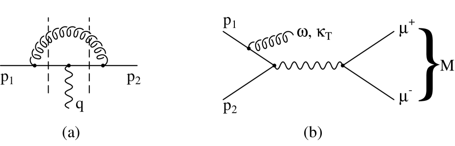
Figure 6: (a) Virtual and (b) real emission contributions to the Drell-Yan process $q(p_{1})\overline{q}(p_{2})\rightarrow\gamma^{*}(q)$.

Let us first recall the origin of the ${\cal O}(\pi^{2}\alpha_{S}/\pi)$ term in the simplest, Drell-Yan, case, which arise from the diagrams of Fig. 6. We first consider the emission of a single soft gluon, shown in Fig. 6b, with energy $\omega$ and transverse momentum $\kappa_{T}$. The probability to emit the gluon is

$$\overline{n}\;=\;4C_{F}\>\int^{\frac{1}{4}M^{2}}\>\frac{d\kappa_{T}^{2}}{\kappa_{T}^{2}}\>\int_{\kappa_{T}}^{\frac{1}{2}M}\>\frac{d\omega}{\omega}\>\frac{\alpha_{S}}{4\pi}\;=\;\frac{\alpha_{S}C_{F}}{4\pi}\>\ln^{2}\>\frac{M^{2}}{\mu^{2}},$$ (59)

where here $M$ is the invariant mass of the Drell-Yan $\mu^{+}\mu^{-}$ pair, and where for simplicity of presentation we ignore, for the moment, the running of $\alpha_{S}(\kappa_{T}^{2})$. Such soft gluons are emitted independently. Summing over all possible emissions, we obtain a Poisson distribution with average multiplicity $\overline{n}$. The normalization factor $\exp(-\overline{n})$ comes from the loop diagrams where the emitted gluon is absorbed by the other quark. The factor is [17]

$$\exp\>\left(-\frac{\alpha_{S}C_{F}}{4\pi}\;\ln\left(\frac{M^{2}}{p^{2}_{1}}\right)\;\ln\left(\frac{M^{2}}{p^{2}_{2}}\right)\right)$$ (60)

where each $\ln(M^{2}/p^{2}_{i})$ contains $i\pi$ from the negative value of the quark virtuality $p^{2}_{i}<0$. Now on taking the sum of the virtual and real gluon emission terms we can obtain the ${\cal O}(\alpha_{S})$ contribution to the cross section for Drell-Yan production. We have

$$\sigma\;=\;\sigma_{0}\>\left(\left|1\>-\>\frac{\alpha_{S}C_{F}}{4\pi}\>\ln^{2}\>\left(\frac{-M^{2}}{\mu^{2}}\right)\right|^{2}\>+\>2\>\frac{\alpha_{S}C_{F}}{4\pi}\>\ln^{2}\>\frac{M^{2}}{\mu^{2}}\right)$$ (61)

where $\sigma_{0}$ is the lowest order cross section and $\mu^{2}\sim|p^{2}_{i}|$. The factor of 2 in the last term arises because the real emission can occur from either the $q$ or the $\overline{q}$ quark. Thus, since $\ln(-M^{2})=\ln M^{2}+i\pi$, the “real” and “virtual” $\alpha_{S}\ln^{2}M^{2}$ cancel and we have

$$\sigma = \sigma_{0}\>\left(1+\frac{\alpha_{S}C_{F}}{2\pi}\>\pi^{2}\>+\>\ldots\right)$$ (62)

$$= \sigma_{0}\>\left(1+{\textstyle\frac{1}{2}}\>\alpha_{S}C_{F}\pi\>+\>\ldots\right)$$

$$\Rightarrow \sigma_{0}\>\exp\left({\textstyle\frac{1}{2}}\>\alpha_{S}C_{F}\pi\right),$$

where the last result corresponds to the resummation of the gluon emissions. If we, as we should, use running $\alpha_{S}(\kappa_{T}^{2})$ in the integral of (59), then we obtain a $\ln(M^{2})\ln(\ln M^{2})$ form. Proceeding as before, and noting $\ln\ln(-M^{2})=\ln\ln M^{2}+(i\pi/\ln M^{2})$, it is straightforward to show that the enhancement factor is such that the Drell-Yan cross section becomes

$$\sigma\;=\;\sigma_{0}\>\exp(\alpha_{S}C_{F}\pi),$$ (63)

with the argument of $\alpha_{S}$ equal to $M^{2}/4$. Note the absence of the factor $\frac{1}{2}$ which occurs in the fixed $\alpha_{S}$ result (62). The larger enhancement is expected since the running of $\alpha_{S}(\kappa_{T}^{2})$ in (59) weights the integrals towards smaller $\kappa_{T}$ values.

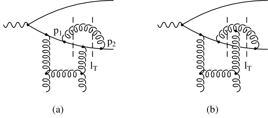
Figure 7: The (virtual) diagrams responsible for the $\pi^{2}$ enhancements to diffractive $c\overline{c}$ production. The exchanged gluon has virtuality $\ell^{2}<0$.

The same $\pi^{2}$ enhancement occurs in diffractive open charm production. It arises (in the Feynman gauge) from the product of the imaginary parts which correspond to the discontinuities indicated by the dashed lines in the diagrams shown in Fig. 7. Here the exchanged gluon has virtuality $\ell^{2}<0$, whereas the quarks have $p^{2}_{i}>0$. Note that $\ell^{2}$ is the counterpart of $M^{2}$ for Drell-Yan production. These are the only graphs which have negative values of the arguments ($\ell^{2}/p^{2}_{i}<0$) of both the logarithms of the counterpart of (60). Without the second $t$-channel gluon (indicated by $\ell_{T}$ in Fig. 7) the diagrams are analogous to ordinary deep inelastic scattering for which there are no large ${\cal O}(\alpha_{S}\pi)$ enhancements. Of course there may be other ${\cal O}(\alpha_{S})$ contributions but these are expected to be much smaller than the $\pi^{2}$ terms. Thus a good estimate of the cross section for diffractive open charm production is

$$\sigma^{c\overline{c}}=\sigma_{0}^{c\overline{c}}\exp(\alpha_{S}C_{F}\pi),$$ (64)

as in Drell-Yan production, but in this case the $\pi^{2}$ enhancement arises from quite different diagrams. For the diffractive process the argument of $\alpha_{S}$ is of the order of the largest mass squared of the quark-gluon state, that is ${\rm max}(p^{2}_{1},p^{2}_{2})$, which is of the order of $k^{2}_{T}+m^{2}$. The largest value is $M^{2}$, where $M$ is the invariant mass of the $c\overline{c}$ system. Here we take $\alpha_{S}(M^{2}/4)$.

The $\pi^{2}$ enhancement encapsulated in (64), which arises from the diagrams of Fig. 7, is not what we would naively expect. In the space-time picture of section 2.1 we showed that the interaction time $\tau_{i}$ of the $c\overline{c}$ pair with the proton is much less than the $\gamma^{*}\rightarrow c\overline{c}$ fluctuation time $\tau_{\gamma}$. We may therefore hope that the corrections of Fig. 7 are suppressed by a factor $\tau_{i}/\tau_{\gamma}\ll 1$. This is indeed true for the contributions coming from the real part of the diagram, but it is not correct for those arising from the imaginary part, that is the crucial $i\pi$ terms. The imaginary part (the discontinuity) of the amplitude corresponds to the possibility of producing a real (not virtual) intermediate state which may live infinitely long. To obtain the imaginary contribution $i\pi\delta(p^{2}-m_{qg}^{2})$ we must integrate over the entire time interval from $\tau=-\infty$ up to $\tau=+\infty$ for the Feynman diagram in the coordinate representation. When we evaluate the discontinuity using the unitarity relation, 2 Im$A=AA^{*}$, in the space-time picture the time in $A^{*}$ goes in the reverse direction to that in $A$. From the formal point of view the inverse direction of time arises from the opposite signs of $i\varepsilon$ in the Feynman propagators $(p^{2}-m_{qg}^{2}\pm i\varepsilon)^{-1}$ of the amplitudes $A$ and $A^{*}$. This point has been discussed in detail in the appendix of a paper by Gribov [18].

Thus the large $K$ factor of $1+{\cal O}(\pi^{2}\alpha_{S}/\pi)$ does not contradict the space-time picture and the factorization properties described in section 2.1. In other words this ${\cal O}(\pi\alpha_{S})$ contribution may be regarded as what is left after the cancellation of the real and virtual gluon emission contributions which occur during the time-like evolution (or parton showering in the final state), which is usually not taken into account, as the leading logarithmic contributions for inclusive cross sections are cancelled.

It is interesting to contrast the enhancement of diffractive open charm production with the situation for diffractive $J/\psi$ production. To calculate the probability for the exclusive $J/\psi$ process we have to convolute the $c\overline{c}$ amplitude ${\cal M}_{\lambda\lambda^{\prime}}$ of (10) with the wave function of the $J/\psi$ meson just after the interaction. Here there is not sufficient time and energy to form a real intermediate quark-gluon state (analogous to the states formed in Fig. 7). Thus we do not expect a large $K$ factor for diffractive $J/\psi$ production. The corrections coming from the loop diagrams may be treated as corrections to the $J/\psi$ wave function (including the possibility of $c\overline{c}g$ states in the $J/\psi$ meson).

We now return to diffractive open charm production, the subject of this paper. We have considered the virtual corrections to $c\overline{c}$ production. For completeness let us also consider the corrections for $c\overline{c}g$ production. In this case we are less able to estimate the enhancement factor. In an important region of phase space the $(c\overline{c})g$ system is produced in a colour octet-octet configuration, with the $t$-channel gluon $\ell$ interacting with the $s$-channel gluon jet, as in Fig. 4a. Similar arguments lead to an enhancement of the form of (63) but with the colour factor $C_{F}$ replaced by $C_{A}$

$$\sigma^{c\overline{c}g}=\sigma_{0}^{c\overline{c}g}\exp(\alpha_{S}C_{A}\pi).$$ (65)

On the other hand if the colour triplet-triplet configuration $c(\overline{c}g)$ is appropriate then the enhancement factor is that given in (63). However, the $c\overline{c}g$ contribution is only appreciable at the large values of $M^{2}$, see section 4, and so the large value (and the large uncertainty) of the enhancement factor does not have serious impact on our main open charm predictions for HERA. To illustrate the ambiguity we show results for two possible enhancements of the $c\overline{c}g$ contribution. First, as an upper limit, we use (65). Then in a crude attempt to allow for the $c(\overline{c}g)$ and $\overline{c}(cg)$ configurations we take

$$\sigma^{c\overline{c}g}\;=\;\sigma_{0}^{c\overline{c}g}\>\left[\frac{1}{3}\>\exp(\alpha_{S}C_{A}\pi)\>+\>\frac{2}{3}\>\exp(\alpha_{S}C_{F}\pi)\right],$$ (66)

which may be regarded as a lower limit.

The exponential enhancement factor for $c\overline{c}$ production in (64) is important. It is typically in the range 2.7–4.0. However (64) is only an estimate of the true $K$ factor. To remove the scale dependence we need to know the two loop diagrams. Even at one loop level only the simplest, although the dominant, contribution (proportional to $\pi^{2}$) is taken into account. Nevertheless experience of the Drell-Yan process leads us to expect that the true $K$ factor is well approximated by the simple expression in (64).

For diffractive $J/\psi$ production we do not have to consider the soft gluon emissions, since they are already included in the normalization of the $J/\psi$ wave function. The ambiguity in the estimates of the relativistic corrections to the wave function [4] is, in a sense, similar to the uncertainty due to the neglect of the higher loop etc. corrections to the simplified expression for the $K$ factor.

4. Numerical estimates of open charm production

We use the QCD formalism developed in the previous two sections to estimate the rate of the diffractive production of open charm from both longitudinally and transversely polarised photons. We discuss both photo- and electro-production.

4.1. A first glimpse of the structure of the $\gamma^{*}\rightarrow c\overline{c}$ diffractive cross sections

Before we present the detailed perturbative QCD predictions for the cross sections for diffractive open charm production it is informative to use the leading logarithmic approximation, (S0.Ex13) and (S0.Ex18), to crudely anticipate some of the general features of the results. An important advantage of the diffractive production of heavy, as opposed to light, quarks is the dominance of small-distance contributions. The $k_{T}$ integrations in (S0.Ex13) and (S0.Ex18) are infrared safe, protected by the mass $m$ of the charm quark. Moreover the scale $K^{2}$ at which the gluon distribution is sampled is [9, 10]

$$K^{2}\;=\;\frac{m^{2}+k_{T}^{2}}{1-\beta}$$ (67)

which may be considerably in excess of $m^{2}$ depending on the value of $\beta$ and the dominant region of $k_{T}^{2}$ sampled. Fig. 8 shows the integrands $I_{L,T}(k_{T}^{2})$ of the integrals in (S0.Ex13) and (S0.Ex18) for various values of $Q^{2}$ and $\beta$ defined such that

$$x_{{I\!\!P}}\>\frac{d\sigma_{L,T}}{dx_{{I\!\!P}}}\;\equiv\;\int_{0}^{\frac{1}{4}M^{2}-m^{2}}\>\frac{dk_{T}^{2}}{\sqrt{1-4m_{T}^{2}/M^{2}}}\;I_{L,T}(k_{T}^{2})$$ (68)

where the cross sections have been integrated over $t$ assuming the form $\exp(-b|t|)$ with slope $b=4$ GeV^-2 [1]. We comment on these plots below.

Figure 8: The $k_{T}^{2}$ integrands $I_{L,T}(k^{2})$, in units of GeV^-4 as defined in (68), occurring in the diffractive open charm cross section formulae, (40) and (41), for $x_{{I\!\!P}}=5\times 10^{-4}$ and various values of $Q^{2}$ and $\beta$. MRS(A^′) partons [19] are used.

For moderate values of $\beta$ ($0.3\lower 3.01385pt\hbox{$\;\stackrel{{\scriptstyle\textstyle<}}{{\sim}}\;$}\beta\lower 3.01385pt\hbox{$\;\stackrel{{\scriptstyle\textstyle<}}{{\sim}}\;$}0.8$) we can obtain from the diffractive cross section formulae in (S0.Ex13) and (S0.Ex18) a rough estimate of the ratio $\sigma_{L}/\sigma_{T}$. We find

$$\sigma_{L}:\sigma_{T} \approx \frac{2\langle m_{T}^{2}\rangle\beta^{3}}{Q^{4}}\;:\;\frac{\beta(1-\beta)^{2}}{Q^{2}}$$ (69)

$$= \frac{2\langle m_{T}^{2}\rangle Q^{2}}{(Q^{2}+M^{2})^{3}}\;:\;\frac{M^{4}}{(Q^{2}+M^{2})^{3}}$$

where $\langle m_{T}^{2}\rangle$ is the average value of $m_{T}^{2}\equiv m^{2}+k_{T}^{2}$ sampled by the integration in (S0.Ex13), and where the factor of 2 in $\sigma_{L}$ comes from an approximate comparison of the integrands of (S0.Ex13) and (S0.Ex18). Eq. (69) not only gives a reasonable estimate of $\sigma_{L}/\sigma_{T}$ (up to a factor of two) but also can be used as a rough guide of the $Q^{2}$ and $M^{2}$ dependence of the individual cross sections — apart, of course, from the $M^{2}$ threshold effect coming from the rapidly expanding kinematic region of integration $(0,\>\frac{1}{4}M^{2}-m^{2})$. From (69) we see that for $\sigma_{L}$ to dominate over $\sigma_{T}$ we have to go to large $Q^{2}$ and small $M^{2}$. For example for $Q^{2}=50$ GeV² and $M^{2}=12$ GeV² we anticipate from (69) that $\sigma_{L}/\sigma_{T}\approx 4Q^{2}m^{2}/M^{4}\approx 3$ whereas if $M^{2}$ is increased to 20 GeV² then $\sigma_{L}\approx\sigma_{T}$. Here we have used $\langle k_{T}^{2}\rangle\approx m^{2}$, see Fig. 8(c), and hence $\langle m_{T}^{2}\rangle\approx 2m^{2}$. These rough estimates of $\sigma_{L}/\sigma_{T}$ are in agreement with the results of the full numerical evaluation of the cross sections (which we will show in Fig. 10).

Figure 9: The average value of $\langle k_{T}^{2}\rangle$ for the integrals in (40) and (41) for $Q^{2}=12$ and $50$ GeV$\,{}^{2}$ and $x_{{I\!\!P}}=5\times 10^{-4}$. The MRS(A^′) gluon is used.

To see the typical values of $k_{T}^{2}$ sampled in the integrations (S0.Ex13) and (S0.Ex18) we calculate the average value of $\ln k_{T}^{2}$. We show the results in Fig. 9 in the form

$$\langle k_{T}^{2}\rangle\;\equiv\;\exp\>\left(\overline{\ln k_{T}^{2}}\right)$$

as a function of $\beta$ for our selected values of $Q^{2}$ and $x_{I\!\!P}$. Unless $\beta$ is small, we see, for both $\sigma_{T}$ and $\sigma_{L}$, that $\langle k_{T}^{2}\rangle$ is of the order of $m^{2}$; as may be expected, for example, from Figs. 8(b,c). Of course as we approach the kinematic bound at $\beta=Q^{2}/(Q^{2}+4m^{2})$, which corresponds to $M^{2}=4m^{2}$, the interval of integration shrinks to zero and hence $\langle k_{T}^{2}\rangle\rightarrow 0$. On the other hand, if we consider large $M^{2}$, so that we have a large interval for the $k_{T}^{2}$ integration in (S0.Ex13), then the integrand $I_{L}$ develops a different character. It is dominated by contributions near the upper end of the region of integration (see, for example, the dashed curve in Fig. 8(a)). It follows that the value of $\langle k_{T}^{2}\rangle$ is nearer the upper limit $\frac{1}{4}M^{2}$ (as shown by the behaviour of the dashed curve in Fig. 9 for small $\beta$). Hence $\sigma_{L}$ samples the gluon at high scales $K^{2}\approx\frac{1}{4}M^{2}$. Unfortunately in this domain the cross section $\sigma_{L}$ is very small.

4.2. Evaluation of the cross sections $\sigma^{L,T}$ for diffractive $c\overline{c}$ production

We calculate the cross sections for the diffractive production of open charm from the QCD formula of (40) and (41) for $c\overline{c}$ production, together with the higher order contributions arising from $c\overline{c}g$ processes of section 3.1 and the $K$ factor of section 3.2. The integrals

$${\cal I}_{i}(k_{T}^{2})\;=\;\int_{0}^{\infty}\>\frac{d\ell_{T}^{2}}{\ell_{T}^{2}}\>\alpha_{S}(\ell_{T}^{2})\>f(x_{I\!\!P},\ell_{T}^{2})\>K_{i}(\ell_{T}^{2},k_{T}^{2})$$ (70)

over the transverse momenta of the exchanged gluons are evaluated numerically, where $\ell_{T}^{2}K_{i}(\ell_{T}^{2},k_{T}^{2})$ are the expressions given in brackets in the formulae (29) and (35) for ${\cal I}_{1}$ and ${\cal I}_{2}$ respectively. The contributions from the infrared region $\ell_{T}^{2}<Q_{0}^{2}$ are evaluated in two alternative ways. We rewrite (70) as

$${\cal I}_{i}\;=\;\alpha_{S}(Q_{0}^{2})\>A_{i}(Q_{0}^{2})\>+\>\int_{Q_{0}^{2}}^{\infty}\>d\ell_{T}^{2}\>\alpha_{S}(\ell_{T}^{2})\>\frac{\partial\biggl{(}x_{I\!\!P}g(x_{I\!\!P},\ell_{T}^{2})\biggr{)}}{\partial\ell_{T}^{2}}\>K_{i}(\ell_{T}^{2},k_{T}^{2}),$$ (71)

where we have used (20) to express the unintegrated distribution in terms of the conventional gluon density. The first estimate of the infrared contribution is made using

$$A_{i}\;=\;x_{I\!\!P}\>g(x_{I\!\!P},Q_{0}^{2})\>K_{i}(0,k_{T}^{2}).$$

We compare this result with that obtained by performing the $0<\ell_{T}^{2}<Q_{0}^{2}$ integration assuming that $\alpha_{S}(\ell_{T}^{2})\>g(x_{I\!\!P},\ell_{T}^{2})=(\ell_{T}^{2}/Q_{0}^{2})\alpha_{S}(Q_{0}^{2})\>g(x_{I\!\!P},Q_{0}^{2})$. The two methods give essentially the same results. We also test the sensitivity of the predictions to variations in the choice of $Q_{0}^{2}$ in the range 0.65 to 1.5 GeV². Again we find that the results are stable.

So far we have calculated the imaginary part of the amplitude, see (17). At high energy $W$, that is small $x_{I\!\!P}$, our positive-signature exchange amplitude behaves as

$$T\>\propto\>i(x_{I\!\!P}^{-\lambda}\>+\>(-x_{I\!\!P})^{-\lambda})$$ (72)

arising from the small $x_{I\!\!P}$ behaviour of the gluon. Provided that $\lambda$ is small, $\lambda\lower 3.01385pt\hbox{$\;\stackrel{{\scriptstyle\textstyle<}}{{\sim}}\;$}0.3$, the amplitude is dominantly imaginary and the real part can be calculated as a perturbation

$$\frac{{\rm Re}T}{{\rm Im}T}\;\approx\;\frac{\pi}{2}\lambda\;\approx\;\frac{\pi}{2}\>\frac{\partial\ln(x_{I\!\!P}g(x_{I\!\!P},\ell_{T}^{2}))}{\partial\ln(1/x_{I\!\!P})}.$$ (73)

We calculate the correction from (73) and allow for a possible dependence of $\lambda$ on the scale $\ell_{T}^{2}$ of the gluon. The contribution of the real part is included in all the predictions shown below.

Figure 10: The cross sections $(x_{{I\!\!P}}d\sigma^{L,T}/dx_{{I\!\!P}})/4\pi^{2}\alpha$ (in GeV$\,{}^{-2}$) for the diffractive production of open charm from longitudinally and transversely polarised photons for $x_{I\!\!P}=5\times 10^{-4}$ and $5\times 10^{-3}$ and $Q^{2}=0,12$ and $50$ GeV$\,{}^{2}$. The continuous and dashed curves correspond to $\sigma_{T}$ and $\sigma_{L}$ respectively. Both the $c\overline{c}$ and $c\overline{c}g$ contributions are shown. The mass of the charm quark is taken to be $m=1.5$ GeV. The MRS(A^′) gluon is used. The predictions are made using (40), (41) and (52), and the “$K$ factor” enhancements of (64), (66) are not included.

The cross sections are shown in Fig. 10 in the form

$$\frac{x_{I\!\!P}}{Q^{2}}F_{i}^{D(3)}\;\equiv\;\frac{1}{4\pi^{2}\alpha}\>x_{I\!\!P}\>\frac{d\sigma^{i}}{dx_{{I\!\!P}}},$$ (74)

with $i=L,T$, after integration over $t$ assuming the form $\exp(-b|t|)$ with the observed value of the slope parameter $b=4$ GeV^-2. Eq. (74) relates the cross sections that are shown in Fig. 10 to the conventional definition of $F^{D(3)}$. The cross sections are plotted as a function of the square of the invariant mass of the $c\overline{c}$ system for six different values of $(x_{{I\!\!P}},Q^{2})$; namely $x_{{I\!\!P}}=5\times 10^{-4}$ and $5\times 10^{-3}$ and $Q^{2}=0,12$ and 50 GeV². The gluon of the MRS(A^′) set of partons [19] is used and the mass of the charm quark is taken to be $m=1.5$ GeV. Throughout this paper we take the running coupling $\alpha_{S}$ to be such that it gives $\alpha_{S}(M_{Z}^{2})=0.118$. The uncertainty $\Delta\alpha_{S}(M_{Z}^{2})=0.005$ translates into typically a $\pm 20\%$ error on the predicted cross sections.

Some of the predictions shown in Fig. 10 are beyond the kinematic reach of the HERA electron-proton collider. For example if we take the maximum $\gamma^{*}p$ energy for which open charm can be measured to be $W=200$ GeV then for $x_{{I\!\!P}}=5\times 10^{-3}$ we see from (4) that $Q^{2}+M^{2}<200$ GeV², whereas for $x_{{I\!\!P}}=5\times 10^{-4}$ we have $Q^{2}+M^{2}<20$ GeV².

Figure 11: The ratio $d\sigma^{L}/d\sigma^{T}$ obtained from Fig. 10.

From Fig. 10 we see that the cross section $\sigma^{T}$ is generally dominant, except for low values of $M^{2}$ at the higher values of $Q^{2}$. This property is clear from Fig. 11 which shows the ratio $d\sigma^{L}/d\sigma^{T}$ as a function of $M^{2}$. Indeed the results for the $c\overline{c}$ contributions shown in Fig. 10 quantify the structure that we anticipated in (69). We notice that the gluon emission contributions $c\overline{c}g$ (of section 3.1) are relatively small for $M^{2}\lower 3.01385pt\hbox{$\;\stackrel{{\scriptstyle\textstyle<}}{{\sim}}\;$}25$ GeV², especially for $Q^{2}\neq 0$.

Figure 12: The cross section $(x_{{I\!\!P}}d\sigma/dx_{{I\!\!P}}$ (in nb) for the diffractive production of open charm obtained from the QCD formulae (40), (41) and (52) using MRS(A^′,G) [19] (continuous, dashed) and GRV [21] (dot-dashed) partons (with $m=1.5$ GeV). The dotted curve corresponds to a charm quark mass $m=1.7$ GeV for the MRS(A^′) gluon. The “$K$ factor” enhancements of (64) and (66) are included.

Fig. 12 shows the sum of all the contributions to the cross section for the diffractive production of open charm for three recent sets of partons MRS(A^′,G) [19] and GRV [21]. The sensitivity to the square of the gluon density is evident. Moreover note that, as anticipated, the sensitivity is greater at the smaller value of $x_{I\!\!P}$. The most recent HERA data for the inclusive proton structure function $F_{2}$ favour MRS(A^′) to GRV but exclude MRS(G). The predictions of Figs. 8–12 correspond to the choice $m=1.5$ GeV for the mass of the charm quark. For comparison the dotted curve in Fig. 12 shows the prediction for $m=1.7$ GeV for the MRS(A^′) gluon.

4.3. The $x_{{I\!\!P}}$ dependence of the cross sections

For diffractive production it is conventional to plot the cross section (integrated over $t$) versus $x_{{I\!\!P}}$ on a $\log-\log$ plot in order to see if there is a universal $x_{{I\!\!P}}^{-n}$ dependence with $n$ independent of $\beta$ and $Q^{2}$. The motivation for studying such a power-like dependence on $x_{{I\!\!P}}$ comes from the Regge inspired approach to diffractive scattering in which $n$ is closely related to the $(t=0)$ intercept of the Pomeron.

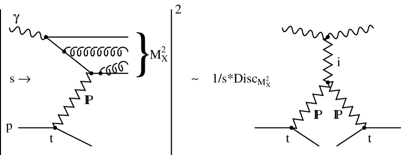
Figure 13: The diffractive cross section for $\gamma^{*}p\rightarrow Xp$ for large $s/M_{X}^{2}$ and large $M_{X}^{2}$ expressed in triple Regge form, where Disc${}_{M_{X}^{2}}$ means the discontinuity is to be taken across the $M_{X}^{2}$ cut of the elastic photon-Pomeron amplitude.

Suppose we were to assume that at high energies our diffractive process is dominated by Pomeron exchange. Then it follows (see Fig. 13) that the cross section for large $s/M_{X}^{2}$ may be written in the form

$$\frac{d\sigma}{dx_{{I\!\!P}}dt}\;\sim\;\sum_{i}\>G_{PPi}(t)\>\left(\frac{s}{M_{X}^{2}}\right)^{2\alpha_{P}(t)-1}\>(M_{X}^{2})^{\alpha_{i}(0)-1}$$ (75)

where the sum is over all Regge exchanges which contribute to photon-Pomeron elastic scattering including the Pomeron itself. This result applies for large $M_{X}^{2}$, but we can reasonably expect the same form with $M_{X}$ replaced by $M$, for large values of the $c\overline{c}$ invariant mass. Recalling that

$$\frac{s}{M^{2}}\;\sim\;\frac{1}{x_{{I\!\!P}}},\hskip 28.45274ptM^{2}\;=\;\frac{Q^{2}}{\beta}\>(1-\beta)$$ (76)

we see that we can rewrite the cross section in the form

$$\frac{d\sigma}{dx_{{I\!\!P}}dt}\;\sim\;F_{2}^{P}(\beta,Q^{2},t)\>\left(\frac{1}{x_{{I\!\!P}}}\right)^{2\alpha_{P}(t)-1}$$ (77)

where $F_{2}^{P}$ can be regarded as the structure function of the Pomeron. The main feature of this Pomeron exchange model is that the power $n=2\alpha_{P}(t)-1$ does not depend on $\beta$ and $Q^{2}$ and so can be treated as a flux factor [22].

It is therefore informative to display our predictions for the diffractive open charm cross sections

$$F_{L,T}^{D(3)}\>(x_{{I\!\!P}},\beta,Q^{2})\;\equiv\;\frac{Q^{2}}{4\pi^{2}\alpha}\>\int\>dt\>\frac{d\sigma^{L,T}}{dx_{{I\!\!P}}dt}$$ (78)

on a $\ln F^{D(3)}$ versus $\ln x_{{I\!\!P}}$ plot to check whether a linear $x_{{I\!\!P}}^{-n}$ form is obtained. The results are shown in Fig. 14 for the values of $\beta$ and $Q^{2}$ that were chosen for Fig. 8. From the figure we see that QCD predicts that the behaviour is only approximately linear. The values of $n$ obtained from the slope of the curves at selected values of $x_{I\!\!P}$ are shown in Table 1. We see that $n$ depends on $Q^{2},\beta$ and also $x_{I\!\!P}$. This is to be expected. For the diffractive production of heavy quarks we can trust the purely perturbative QCD calculation based on two-gluon exchange; we are not in the regime of (non-perturbative or “soft”) Pomeron exchange where $n=2\alpha_{P}(\overline{t})-1$.

Table 1: The exponents $n$ of the effective $x_{I\!\!P}^{-n}$ behaviour of $F^{D(3)}$ at different values of $x_{I\!\!P},Q^{2}$ and $\beta$. $Q^{2}$ is given in GeV².

	$Q^{2}=12$,	$\beta=0.1$	$Q^{2}=12$,	$\beta=0.4$	$Q^{2}=50$,	$\beta=0.7$
$x_{I\!\!P}$	$n_{T}$	$n_{L}$	$n_{T}$	$n_{L}$	$n_{T}$	$n_{L}$
$3\times 10^{-4}$	1.40	1.31	1.48	1.52	1.53	1.56
$10^{-3}$	1.38	1.31	1.48	1.53	1.52	1.56
$3\times 10^{-3}$	1.38	1.31	1.53	1.59	1.59	1.63
$10^{-2}$	1.43	1.39	1.54	1.59	1.59	1.63

Figure 14: Plots of $F^{D(3)}(x_{{I\!\!P}},\beta,Q^{2})$, defined in (78), versus $x_{{I\!\!P}}$ for the values of $\beta$ and $Q^{2}$ used in Fig. 8. As usual the continuous (dashed) curves correspond to $F_{T}(F_{L})$. The values of the exponent $n$ of $F^{D(3)}\sim x_{{I\!\!P}}^{-n}$ are listed in Table 1.

4.4. The diffractive structure function $F_{2}^{D(2)}$(charm)

It is also useful to introduce the diffractive structure function integrated over $x_{{I\!\!P}}$ (as well as $t$)

$$F_{2}^{D(2)}\>(\beta,Q^{2})\;\equiv\;\frac{Q^{2}}{4\pi^{2}\alpha}\>\int_{x_{1}}^{x_{2}}\>\frac{d\sigma}{dx_{{I\!\!P}}}\>dx_{{I\!\!P}}$$ (79)

which would be the charm component of the Pomeron structure function in the Pomeron exchange model approach. Even though we have seen that there is no basis for this model, it is still possible to write an evolution equation, similar to GLAP evolution, which gives the $\beta$ and $Q^{2}$ dependence of $F_{2}^{D(2)}$ [12, 23]. Note that the integral over $\beta$ of $F_{2}^{D(2)}$ gives the contribution of diffractive charm production to the total deep inelastic cross section and is intimately related to the shadowing corrections to the deep inelastic structure function.

Figure 15: The continuous and broken curves are the predictions for the contribution of diffractive open charm production to the structure function $F_{2}^{D(2)}(\beta,Q^{2})$ of (79) as a function of $\beta$ for $Q^{2}=12$ and $50$ GeV$\,{}^{2}$ respectively. The MRS(A^′) gluon is used. $x_{{I\!\!P}}$ is integrated over the interval ($0.0003$, $0.05$). The curves branch at low values of $\beta$ according to whether we use the enhancement factor (65) or (66) arising from the virtual corrections to $c\overline{c}g$ production.

In Fig. 15 we show the predictions for $F_{2}^{D(2)}$ as a function of $\beta$ for $Q^{2}=12$ and 50 GeV². We take the limits of the integration in (79) to be $x_{1}=0.0003$ and $x_{2}=0.05$ so as to be able to compare our predictions for $F_{2}^{D(2)}$(charm) with the experimental measurements [24] for the total diffractive structure function (which includes light quark production as well as charm). The experimental data at $Q^{2}=12$ GeV² give values of $F_{2}^{D(2)}$(total) in the range 0.15–0.2, approximately independent of $\beta$. At $Q^{2}=50$ GeV² the measured values are $F_{2}^{D(2)}$(total) $\simeq 0.3$ (0.2) at $\beta=0.2$ (0.65), but again compatible within the errors with no $\beta$ dependence. These are the values obtained by the H1 collaboration [24]. Similar results are found by the ZEUS collaboration [25]. We thus see from Fig. 15 that in this kinematic range the open charm contribution is predicted to be approximately 25–30% of the measured diffractive structure function. The results shown in Fig. 15 are obtained using MRS(A^′) partons and the mass of the charm quark $m=1.5$ GeV. If a mass $m=1.7$ GeV were to be used then the height of the peaks shown in Fig. 15 would be reduced by 20%. If on the other hand GRV or MRS(G) partons are used then the peak value of $F_{2}^{D(2)}$(charm) at $Q^{2}=50$ GeV² is found to be 0.17 or 0.24 respectively, as compared to 0.074 for MRS(A^′). When compared with the experimental values of $F_{2}^{D(2)}$(total), these high values of $F_{2}^{D(2)}$(charm) clearly disfavour the small $x$ gluon distributions of these sets of partons, even allowing for the uncertainty in the $K$ factor enhancement (64) or due to the choice of $m$.

Fig. 15 displays clearly the characteristic $\beta$ dependence of diffractive open charm production. First we see the kinematic bound for $c\overline{c}$ production. It corresponds to an upper limit on $\beta$,

$$\beta_{\rm max}\;=\;\frac{Q^{2}}{Q^{2}+M_{th}^{2}}$$ (80)

where the threshold mass is given by $M_{th}^{2}=4m^{2}$. The peak seen just below this value of $\beta$ arises from $c\overline{c}$ production just above threshold with a fall off as $M^{2}$ increases (i.e. $\beta$ decreases). The rise which occurs for smaller $\beta$ corresponds to $c\overline{c}g$ production. Recall that for the $c\overline{c}g$ component there is a large enhancement arising from virtual corrections to this process. The size of the enhancement is not well known. This uncertainty in the $c\overline{c}g$ contribution is represented in Fig. 15 by two curves which correspond to two different choices, (65) and (66), of the $c\overline{c}g$ enhancement $K$ factor. Indeed at the lowest value of $\beta$ shown (for each $Q^{2}$), after the $c\overline{c}$ contribution is subtracted, we find that the residual $c\overline{c}g$ contribution has approximately a factor of two uncertainty.

5. Conclusions

We have presented the QCD predictions for the cross sections $(\sigma_{L,T})$ for the diffractive production of open charm from longitudinally and transversely polarised photons of virtuality $Q^{2}$. At lowest order, the diffractive processes $\gamma^{*}p\rightarrow c\overline{c}p$ are driven by two-gluon exchange between the $c\overline{c}$ pair and the proton. The perturbative predictions are protected by the mass $m$ of the charm quark and are infrared safe. In fact the diffractive production of open charm depends on the square of the gluon density $x_{I\!\!P}g(x_{I\!\!P},K^{2})$, with $x_{I\!\!P}=(Q^{2}+M^{2})/s$ at a scale

$$K^{2}\;=\;\left(\langle k_{T}^{2}\rangle\>+\>m^{2}\right)\;\left(1\>+\>\frac{Q^{2}}{M^{2}}\right)$$ (81)

where typically $\langle k_{T}^{2}\rangle\sim m^{2}$. $M$ is the invariant mass of the $c\overline{c}$ system.

We have aimed to make our diffractive cross section predictions as realistic as possible for the experiments at HERA. We have studied the $Q^{2}$ and $M^{2}$ dependence of both $\sigma_{L}$ and $\sigma_{T}$. We found that $\sigma_{L}$ only exceeds $\sigma_{T}$ in the kinematic region of low $M^{2}$ and high $Q^{2}$. There are several new features incorporated in our analysis. First, we integrate explicitly over the transverse momenta $\pm\mbox{\boldmath$\ell$}_{T}$ of the exchanged gluons. This proves to be important, since we find that the inclusion of the $\ell_{T}^{2}$ effects increases the cross sections by about a factor of 2 as compared to using just the leading logarithmic approximation. Second, we have estimated the higher-order contributions to diffractive open charm production. These were divided into the computation of real emission $c\overline{c}g$ contributions, and the estimation of the enhancement due to virtual corrections to $c\overline{c}$ production. The real gluon emission contributions were found to be small for low $M^{2}$, $M^{2}\lower 3.01385pt\hbox{$\;\stackrel{{\scriptstyle\textstyle<}}{{\sim}}\;$}25$ GeV², and moreover decrease with increasing $Q^{2}$. The virtual corrections on the other hand, are surprisingly important. They arise from the diagrams of Fig. 7, and have some similarities to the $\pi^{2}$ enhancement of the ${\cal O}(\alpha_{S})$ corrections that is well-known in Drell-Yan production. However, their occurrence in diffractive $\gamma^{*}\rightarrow c\overline{c}$ production is a novel and theoretically interesting effect. To a good approximation they can be resummed and represented by a $K$ factor enhancement in the form of an exponential with argument ${\cal O}(\alpha_{S}\pi)$. Just as in Drell-Yan production, we estimate an enhancement of the lowest-order result by a factor of about 3. Due to the larger colour coupling of the gluon, the enhancement is expected to be greater for the $c\overline{c}g$ contribution. However, in this case the $K$ factor is not well-known. Thus in the large $M^{2}$ (and small $Q^{2}$) region, where the $c\overline{c}g$ contribution is not negligible, our cross section predictions have a larger uncertainty (as represented, for example, by the branching of the curves shown in Fig. 15 at the lower value of $\beta$).

We have used the above perturbative QCD formalism to calculate the cross sections $\sigma_{L,T}$ for diffractive open charm production. We have presented representative numerical results to illustrate the $Q^{2}$, $M^{2}$ and $x_{I\!\!P}$ dependence of the cross sections, which are relevant to the experiments at HERA. In particular we show the sensitivity to the choice of gluon distribution at small $x$.

We may compare diffractive open charm production with diffractive $J/\psi$ production at HERA. Both processes are special in that they depend quadratically on the gluon distribution at small $x$. The main uncertainty in the calculation of the cross section for diffractive $J/\psi$ production was found to be associated with the Fermi motion of the $c$ and $\overline{c}$ within the $J/\psi$ and the choice of the mass $m$ of the charm quark [4, 5]. The uncertainty is greater in the predicted size of the cross section than in the energy (or equivalently the $x$) dependence of the cross section. That is the shape, rather than the normalization, of the observed cross section is a better discriminator between the various gluon distributions. The shape of the diffractive $J/\psi$ photoproduction data collected at HERA favours the MRS(A^′) gluon relative to that of GRV, and rules out the MRS(G) gluon [4].

Diffractive open charm production has the advantage that it is independent of the uncertainties due to the $J/\psi$ wave function. On the other hand the higher order corrections to open charm have (novel) $\pi^{2}$ enhancements which lead to a large $K$ factor which, at present, can only be estimated. The $K$ factor uncertainty is not expected to be present in the $J/\psi$ prediction; it is automatically subsummed by using the observed leptonic width to fix the $J/\psi$ coupling. High energy data for the two processes will therefore act as complementary and independent probes of the gluon at small $x$. Their quadratic sensitivity to the gluon means that valuable information can already be obtained despite the above uncertainties.

When we compared our perturbative QCD predictions for diffractive open charm production with the inclusive data for diffractive production, at a given $\beta$ and $Q^{2}$, we estimate that about 25–30% of diffractive events arise from $c\overline{c}$ production (if the MRS(A^′) gluon is used). The $\beta$ (and $Q^{2}$) dependence of diffractive $c\overline{c}$ production has special features that are well-illustrated in the sample results shown in Fig. 15. Low mass $c\overline{c}$ production leads to a characteristic peak in the region $\beta\lower 3.01385pt\hbox{$\;\stackrel{{\scriptstyle\textstyle<}}{{\sim}}\;$}Q^{2}/(Q^{2}+4m^{2})$, while $c\overline{c}g$ production only becomes important at much lower $\beta$. To identify the dramatic threshold behaviour it will be necessary to reconstruct the mass of the $c\overline{c}$ system.

In summary we have used perturbative QCD to predict diffractive open charm production at HERA as a function of $Q^{2}$, $M^{2}$ and $x_{I\!\!P}$. The main unknowns are (i) the gluon distribution at small $x_{I\!\!P}$, (ii) the mass $m$ of the charm quark and (iii) the accuracy of the estimate of the large $K$ factor enhancement. The quadratic sensitivity to (i) means that information on the gluon can still be obtained despite the ambiguities arising from (ii) and (iii). If the gluon is determined at small $x$ by independent means, then the characteristic $Q^{2}$, $M^{2}$ and $x_{I\!\!P}$ dependence of diffractive $c\overline{c}$ production will offer a valuable probe of the validity of perturbative QCD at $x_{I\!\!P}\lower 3.01385pt\hbox{$\;\stackrel{{\scriptstyle\textstyle<}}{{\sim}}\;$}10^{-3}$ and at scales of the order of a few times $m^{2}$.

Acknowledgements

We thank R. G. Roberts, A. Kataev, V. A. Khoze, P. J. Sutton and T. K. Gehrmann for useful discussions. We thank the UK Particle Physics and Astronomy Research Council and the Royal Society for support, and Grey College of the University of Durham for their warm hospitality. This research was also supported in part (EML) by CNPq of Brazil and in part (MGR) by the Russian Fund of Fundamental Research 96 02 17994.

References

[1] H1 collaboration: S. Aid et al., DESY preprint
96-037;
ZEUS collaboration: M. Derrick et al., Phys. Lett. B350
(1995) 120.
[2] M. G. Ryskin, Z. Phys. C57 (1993) 89.
[3] S. Brodsky et al., Phys. Rev. D50 (1994)
3134.
[4] M. G. Ryskin, R. G. Roberts, A. D. Martin
and E. M. Levin, Durham preprint DTP/95/96.
[5] L. Frankfurt, W. Koepf and M. Strikman, Tel-Aviv
University preprint, TAUP-2290-95.
[6] S. Brodsky and P. Lepage, Phys. Rev. D22
(1980) 2157.
[7] A. H. Mueller, Nucl. Phys. B335 (1990) 115.
[8] N. N. Nikolaev and B. G. Zakharov, Z. Phys. C53 (1992) 331.
[9] J. Bartels, H. Lotter and M. Wüsthoff, DESY
preprint 96-026.
[10] M. Genovese, N. N. Nikolaev and B. G. Zakharov,
hep-ph/9603285.
[11] N. N. Nikolaev and B. G. Zakharov, Z. Phys. C49
(1991) 607;
Phys. Lett. B260 (1991) 414.
[12] E. M. Levin and M. Wüsthoff, Phys. Rev. D50 (1994) 4306.
[13] M. Glück and E. Reya, Phys. Lett. B83
(1979) 98.
[14] E. Witten, Nucl. Phys. B104 (1976) 445.
[15] M. Glück, E. Reya and M. Stratmann, Nucl. Phys. B422 (1994) 37.
[16] J. Kubar-Andre and F. E. Paige, Phys. Rev. D19
(1979) 221;
G. Altarelli, R. K. Ellis and G. Martinelli, Nucl. Phys. B143
(1978) 521;
ibid. B157 (1979) 461.
[17] V. V. Sudakov, JETP 3 (1956) 65.
[18] V. N. Gribov, Sov. Phys. JETP 57 (1970) 709.
[19] A. D. Martin, R. G. Roberts and W. J. Stirling, Phys. Lett. B354 (1995) 155.
[20] H1 collaboration: S. Aid et al., DESY preprint 96-037.
[21] M. Glück, E. Reya and A. Vogt, Z. Phys. C67 (1995) 433.
[22] G. Ingelman and P. Schlein, Phys. Lett. B152 (1985) 256.
[23] T. Gehrmann and W. J. Stirling, Z. Phys. C70 (1996) 89.
[24] H1 collaboration: T. Ahmed et al., Phys. Lett. B348 (1995) 681.
[25] ZEUS collaboration: M. Derrick et al., Z. Phys. C68 (1995) 569.