We review recent efforts to explore the information on masses of heavy matter particles, notably of the top quark and the Higgs boson, as encoded at the quantum level in the renormalization group equations. The Standard Model (SM) and the Minimal Supersymmetric Standard Model (MSSM) are considered in parallel throughout.
First, the question is addressed to which extent the infrared physics of the “top-down” renormalization group flow is independent of the ultraviolet physics. The central issues are i) infrared attractive fixed point values for the top and the Higgs mass, the most outstanding one being $\mbox{$m_{t}$}=O(190\mbox{$\,{{\rm GeV}}$})\sin\beta$ in the MSSM, ii) infrared attractive relations between parameters, the most prominent ones being an infrared fixed top-Higgs mass relation in the SM, leading to $m_{H}$=O(156$\,{{\rm GeV}}$) for the experimental top mass, and an infrared fixed relation between the top mass and the parameter $\tan\beta$ in the MSSM, and iii) a systematical analytical assessment of their respective strengths of attraction. The triviality and vacuum stability bounds on the Higgs and top masses in the SM as well as the upper bound on the mass of the lightest Higgs boson in the MSSM are reviewed. The mathematical backbone for all these features, the rich structure of infrared attractive fixed points, lines, surfaces,… in the corresponding multiparameter space, is made transparent. Interesting hierarchies emerge: i) infrared attraction in the MSSM is systematically stronger than in the SM, ii) generically, nontrivial higher dimensional fixed manifolds are more strongly infrared attractive than the lower dimensional ones.
Tau-bottom-(top) Yukawa coupling unification as an ultraviolett symmetry property of supersymmetric grand unified theories and its power to focus the “top-down” renormalization group flow into the IR top mass fixed point and, more generally, onto the infrared fixed line in the $m_{t}$-$\tan\beta$-plane is reviewed.
The program of reduction of parameters, a systematic search for renormalization group invariant relations between couplings, guided by the requirement of asymptotically free couplings in the complementary “bottom-up” renormalization group evolution, is summarized; its interrelations with the search for IR attractive fixed manifolds are pointed out.

Table of Content

1. Introduction
2. Theoretical framework
      2.1 Standard Model
      2.2 Minimal Supersymmetric Standard Model
      2.3 Grand Unification
      2.4 Renormalization Group Equations
      2.5 Relations between Pole Masses and $\overline{{\rm MS}}$ Couplings
      2.6 Effective Potential and Vacuum Stability
3. Preview of Infrared Fixed Manifolds and Bounds in the SM and MSSM
4. Infrared Fixed Points, Lines, Surfaces and Mass Bounds
4. in Absence of Electroweak Gauge Couplings
      4.1 The Pure Higgs Sector of the SM – Triviality and an Upper Bound on the Higgs Mass
      4.2 The Higgs-Top Sector of the SM - a First IR Fixed Line and a First Vacuum Stability       4.5 Bound
      4.3 The Top-$g_{3}$ Sector of the SM and MSSM – a Non-Trivial IR Fixed Point
      4.4 The Higgs-Top-$g_{3}$ Sector of the SM – a First Non-Trivial Approximation
      4.5 The Top-Bottom-$g_{3}$ Sector of the SM and MSSM – Top-Bottom Yukawa Unification as
      4.5 an IR fixed Property
      4.6 The Higgs-Top-Bottom-$g_{3}$ Sector of the SM – a First IR Fixed Surface
5. Infrared Fixed Points, Lines, Surfaces
5. in Presence of All Gauge Couplings
      5.1 The Top Sector of the SM and MSSM
      5.2 The Top-Bottom-Sector of the SM and MSSM
      5.3 The Higgs-Top-Bottom Sector of the SM
6. Infrared Attractive Top and Higgs Masses, Mass Relations and Mass Bounds
      6.1 Top Mass and $\tan\beta$ in the MSSM
      6.2 Top and Higgs Masses and Top-Higgs Mass Relation in the SM
      6.3 Lower Bound on the Higgs Mass in the SM
      6.4 Upper Bound on the Lightest Higgs Mass in the MSSM
7. Supersymmetric Grand Unification Including Yukawa Unification
8. Program of Reduction of Parameters
9. Conclusions

1 Introduction

The Standard Model (SM) is highly successful at describing the electromagnetic, weak and strong gauge interactions among the elementary particles up to presently accessible energies. It has, however, a conceptual weakness: the masses of the matter particles, i.e. of the quarks, leptons and the theoretically predicted Higgs boson, enter as free parameters. This deficiency largely persists in prominent extensions of the SM, i) its embedding into an underlying grand unified theory (GUT), unifying the three gauge interactions in a single one, ii) its extension by the fermion-boson supersymmetry which is considered to be instrumental for an additional implementation of gravity.

Starting point for this review are investigations of the quantum effects in the framework of this wide class of theories, which have been performed over the last decade or so, with peak activities during the last few years. The main interest focuses on the inherent potential of the quantum effects for i) relating ultraviolet (UV) physics issues to infrared (IR) physics and vice versa and in particular for ii) providing informations on (at least the heavy) particle masses. In their mildest form these informations imply upper and lower bounds for (heavy) particle masses. Ultimatively, however, there even appears to open up the fascinating possibility that one does not have to go beyond the SM and its extensions in search for the dynamical origin of (heavy) particle masses but that this dynamical origin is provided on the level of the quantum effects – in a sense to be specified below.

The top quark and the Higgs boson are the heaviest matter particles of the Standard Model. Only recently the top quark has been observed directly at the proton-antiproton collider at FERMILAB

$${\rm CDF\ collaboration\cite[cite]{[\@@bibref{}{cdf}{}{}]}:}\;\;\;\;\;\mbox{$m_{t}$} = 176\;\pm 8\;\;({\rm stat.})\pm 10\;({\rm syst.})\;\mbox{$\,{{\rm GeV}}$},$$ (1)

$${\rm D0\ collaboration\cite[cite]{[\@@bibref{}{d0}{}{}]}:}\;\;\;\;\;\mbox{$m_{t}$} = 199\begin{array}[]{l}+19\\ -21\\ \end{array}({\rm stat.})\pm 22\;({\rm syst.})\;\mbox{$\,{{\rm GeV}}$}.$$ (4)

This mass value is in good agreement with the present indirect evidence from the electron-positron collider LEP at CERN [3]

$${\rm LEP\ collaborations,\ combined:}\;\;\;\;\;\mbox{$m_{t}$}\;=\;178\begin{array}[]{l}+11+18\\ -11-19\\ \end{array}\mbox{$\,{{\rm GeV}}$};$$ (5)

the central value and the first errors quoted refer to a Higgs mass of 300 $\,{{\rm GeV}}$, the second errors correspond to a variation of the central value when varying the Higgs mass between 60 $\,{{\rm GeV}}$ and 1000 $\,{{\rm GeV}}$. The top quark is much heavier than all the other quarks and leptons, even substantially heavier than its partners in the heaviest fermion generation, the bottom quark with mass

$$\mbox{$m_{b}$}=4.25\pm 0.15\mbox{$\,{{\rm GeV}}$}\,$$ (6)

(the $\overline{\rm MS}$ mass at $\mu=\mbox{$m_{b}$}$) as determined [4] from QCD sum rules, and the tau lepton with mass [5]

$$\mbox{$m_{\tau}$}=1.7771\begin{array}[]{l}+0.0004\\ -0.0005\\ \end{array}\mbox{$\,{{\rm GeV}}$},$$ (7)

which will also play a role in this review.

For the Higgs mass there exits only an experimental lower bound from LEP [5]

$$\mbox{$m_{H}$}>58.4\mbox{$\,{{\rm GeV}}$}$$ (8)

at $95\%$ confidence level. From the upgrade LEP200 of LEP and the future collider LHC one expects soon an extended experimental reach for the Higgs boson. In expectation of these future Higgs searches the activities for a precise determination of theoretical bounds on the Higgs mass have increased in the recent literature [6]-[28], where Ref. [7] has played the role of a primer in the field. This applies in particular to a lower (vacuum stability) bound within the SM and to an upper bound for the lightest Higgs boson within the minimal supersymmetric extension of the SM, the MSSM. The upshot of these developments will be included in this review.

Altogether, one may expect the top and Higgs masses to be very roughly of the order of the weak interaction scale

$$v/\sqrt{2}\simeq 174\mbox{$\,{{\rm GeV}}$},$$ (9)

given in terms of the vacuum expectation value $v$ of the Higgs field. Clearly, it is a great challenge to understand the dynamical origin for why the top and Higgs masses should be of $O(v)$ and also for the mass disparity with respect to the other quarks and leptons. As mentioned already, important clues for an answer lie in the wealth of informations on the top quark and Higgs boson masses, which have emerged from analyses of the quantum effects over the last decade.

In all the above mentioned frameworks of the SM, possibly embedded in a grand unified theory and possibly endorsed with supersymmetry, the Higgs mass and the quark and lepton masses are related to couplings; these couplings are a measure for the strength of the Higgs self interaction and the Higgs-fermion-antifermion Yukawa interactions, respectively. A characteristic signature of the quantum effects is that these couplings are not constant but “run” as functions of a momentum scale $\mu$. The running is encoded in the renormalization group equations (RGE), a set of nonlinear coupled differential equations. They describe the response of all couplings of the theory, the Higgs and Yukawa couplings as well as the electromagnetic, weak and strong gauge couplings, to a differential change in the momentum scale $\mu$. They have been calculated in two-loop order in the framework of perturbation theory. The RGE allow to relate physics at different momentum scales $\mu$. Of interest in this review are scales generically between an infrared (IR) scale of the order of the presently accessible weak interaction scale (9) and some ultraviolet (UV) scale $\Lambda$. Let us emphasize that throughout this review the notions IR scale, IR region or IR behaviour refer to the scale $\mu\simeq v$ and not to the limit $\mu\rightarrow 0$. The UV scale may be as large as $\mbox{$\Lambda$}=\mbox{$M_{{\rm GUT}}$}\simeq O(10^{16}\mbox{$\,{{\rm GeV}}$})$ in the framework of (supersymmetric) grand unification, in which the theory is supposed to continue to hold up to the scale $M_{{\rm GUT}}$ where the three gauge couplings unify, or ultimatively as large as the Planck scale $\mbox{$\Lambda$}=M_{{\rm Planck}}\simeq 10^{19}\mbox{$\,{{\rm GeV}}$}$, where graviational interactions become important.

Let us anticipate and emphasize already here that whichever the framework, SM or its minimal supersymmetric extension (MSSM), and whichever the size of $\Lambda$, the interplay between IR and UV physics and the implications for particle masses turn out to be similar in principle, even though different on the quantitative level. This makes it a challenging task to consider all these cases simultaneously and treat them in parallel, as intended in this review.

In solving the RGE, which are a set of first order differential equations, in the first instance one faces the same inherent deficiency as on the classical level: the initial values of the couplings and thus the particle masses are still free parameters.

There are, however, strong physical motivations from different sources to be spelt out below, which in essence tend to single out special solutions of the RGE. From the mathematical point of view these special solutions are distinguished by being determined by suitable boundary conditions in contradistinction to initial value conditions.

The theoretical motivations in the literature pointing towards such special solutions of the RGE are the following.

• Consider the so-called “top-down” RG evolution, from the UV scale $\Lambda$ to the IR scale. Determine the corresponding RG flow, which comprises all solutions of the RGE for any UV initial values for the Higgs self coupling and the Yukawa couplings which are admitted within the framework of perturbation theory. An important issue [29], [6], [7], [30]-[65], [118], [119] has recently been to determine the extent to which the IR physics is independent of the UV physics, i.e. independent of the UV initial values. This happens if the IR behaviour is dominated by special solutions of the RGE

  • which correspond to fixed points, fixed lines, fixed surfaces,…, in general to fixed manifolds in the space of ratios of couplings,

  • which are IR attractive for the whole RG flow.

  Indeed a rich structure of such IR attractive fixed points, lines, surfaces,… exists, singling out IR attractive top and Higgs mass values and IR attractive relations between masses. The most conspicuous IR fixed point and line with the widest coverage in the literature [43]-[48], [49]-[65], [118], [119] leads within the MSSM to a top mass value of

  $$\mbox{$m_{t}$}\simeq{\rm O}(190-200\mbox{$\,{{\rm GeV}}$})\sin\beta$$ (10)

  and to a fixed line in the $\tan\beta$-$m_{t}$-plane, where $\tan\beta$ is a ratio of two vacuum expectation values characteristic for the Higgs sector of the MSSM. The top mass value (10) is well compatible with the experimental value (4). Within the SM the corresponding IR fixed point leads, though less conspicuously, to a mass value O(215$\,{{\rm GeV}}$), not too far from the experimental value, and the IR fixed point Higgs mass value also of O(210$\,{{\rm GeV}}$). Furtherreaching results are IR attractive relations between the top and Higgs mass or, more generally, between the top, Higgs and bottom masses within the SM and an IR attractive relation between the top mass and $\tan\beta$. Within the SM e.g. an IR attractive top-Higgs mass relation leads to

  $$\mbox{$m_{H}$}=O(156\mbox{$\,{{\rm GeV}}$})\ \ \ \ {\rm for\ the\ experimental\ value}\ \ \ \mbox{$m_{t}$}=176\mbox{$\,{{\rm GeV}}$}.$$ (11)

  These mass values are clearly interesting and make the research into IR fixed manifolds of the RG equations a very appealing subject.

  Let us also anticipate two interesting (phenomenological) hierarchies in the IR attraction of the RG flow which emerge from the presentation of the material in this review.: i) Typically the RG flow is roughly first attracted towards a fixed surface, say, then within this surface along a fixed line and finally along this line towards the fixed point. Now, it turns out that the higher dimensional manifolds imply always highly non-trivial relations between the involved couplings. This pattern of course enhances the importance of higher dimensional IR fixed manifolds. A further interesting hierarchy emerges in the comparison of the SM with the MSSM: the IR fixed manifolds in the MSSM seem to be systematically more strongly attractive than in the corresponding SM ones.

  IR fixed manifolds may be considered to be interesting in their own right, since they correspond to RG invariant values for couplings or to RG invariant relations between couplings and thus between particle masses. Their significance is certainly enhanced if the IR attraction is sufficiently strong as to attract the RG flow into their close vicinity. Of course the RG flow comes the closer to the IR fixed manifold the longer is the evolution path from the UV to the IR. This explains an interest into high UV scales in this context, even though the IR fixed manifolds themselves are independent of the UV scale.

  Next, let us place the well-studied upper (triviality) and lower (vacuum stability) bounds for the Higgs mass and the top mass in context with IR attractive fixed manifolds and the RGE “top-bottom” flow towards them. The existence of these bounds may be traced back to the most strongly IR attractive fixed manifold and the shape of these bounds in the multiparameter space strongly reflects the position of this IR attractive manifold. In fact, since the evolution path from the UV to the IR is finite, there are IR images of UV initial values which fail to reach the most strongly IR attractive manifold; it is their boundaries which constitute the bounds. Clearly the bounds will be the tighter the longer is the evolution path, i.e. the higher is the UV scale. The bounds are thus straight consequences of the perturbatively calculated quantum effects. In certain approximations they are supported by non-perturbative lattice calculations which will also be included in this review. The bounds to be discussed are the so-called triviality bound, a top-mass dependent upper Higgs mass bound, and the vacuum stability bound a top-mass dependent lower Higgs mass bound or, conversely, a Higgs-mass dependent upper top mass bound. As has already been mentioned earlier, the bounds on the Higgs mass in the SM, resp. on the lightest Higgs mass in the MSSM, are of high actuality in view of the search for the Higgs at LEP200 and LHC in the near future and the ongoing efforts to pin down the top mass at FERMILAB.

• A second issue [49]-[65] of high recent interest in the context of the “top-down” RG evolution runs under the headline Yukawa coupling unification;

  • One access is within supersymmetric grand unification. It starts from the very appealing and economical symmetry property of some grand unified models to provide a unification of the tau-bottom or even furtherreaching of the tau-bottom-top Yukawa couplings at the UV grand unification scale $\Lambda$=$M_{{\rm GUT}}$ accompanying the unification of the gauge couplings. In the first instance it does not single out a special solution of the RGE in the sense proclaimed above. It rather furnishes symmetry relations between UV initial values, thus reducing the number of free parameters in the “top-down” RG flow. As it turns out i) this constrained RG flow [49]-[65] focuses in the IR region much more closely onto the IR attractive fixed point and line than the unconstrained one; ii) it appears to be the very existence of the IR attractive fixed point and line which allows the implementation of tau-bottom Yukawa unification.

  • Another access is the observation that there exists an IR attractive fixed manifold which implements approximate top-bottom Yukawa coupling unification at all scales $\mu$, which again is only of interest in the supersymmetric theory, the MSSM.

• The complementary approach is the so-called “bottom-up” evolution of the RGE, from the IR scale up to some UV scale $\Lambda$ (and mathematically also to $\mu\rightarrow\infty$), the direction of evolution advocated by the interesting so-called program of reduction of parameters. The central issues are to establish renormalization group invariant relations (in principle to all orders in perturbation theory) between as many couplings as possible such that ii) they become simultaneously asymptotically free. The program as applied to the SM amounts to a systematic search for special solutions of the RGE which link the top Yukawa coupling and the Higgs self coupling in such a way to the strong gauge coupling that they decrease simultaneously towards zero, i.e. become simultaneously asymtotically free. It should be emphasized that this approach has been the first to concentrate on a systematic search for special solutions of the RGE, subject to the implementation of asymptotic freedom; and it certainly has influenced later developments in the systematic search for special solutions of the RGE, subject to being IR attractive.

There are interesting interrelations between the results from the different approaches:

• among the special solutions of the RGE which are singled out as IR attractive (at the one-loop level) in the “top-down” approach are solutions which implement asymptotic freedom within the “bottom-up” approach and vice versa;

• supersymmetric grand unified theories with additional features like the tau-bottom Yukawa unification or parameter reduction beyond the grand unification scale $M_{{\rm GUT}}$ drive the RG flow into the IR fixed manifolds;

• top-bottom Yukawa coupling unification may be viewed as an UV symmetry input, as motivated from grand unified theories, it also appears to be encoded in an IR attractive fixed manifold which implies approximate top-bottom Yukawa unification at all scales $\mu$.

Thus, different aspects pointing towards special solutions of the RGE may be viewed as different facets of some global regularities in the interplay between IR and UV physics. This is a strong incentive to review all these issues under the same headline as intended in this review.

Altogether, it is clearly a fascinating task to trace to which extent the quantum effects encoded in the RGE for couplings yield information about the Higgs, top and further quark and lepton masses and to which extent IR and UV physics issues are interlocked.

Let us next further specify the scope within which these questions are addressed.

First, a physical interpretation of the UV scale $\Lambda$ is required. In the framework of the SM it is the scale at which new physics beyond the SM is encountered. Generically it is envisaged that the SM is embedded in a more complete underlying theory at a higher momentum scale $\Lambda$; accordingly the SM can be viewed as an effective theory with $\Lambda$ acting as the UV cutoff. The UV scale will presumably be smaller than the Planck mass $\mbox{$\Lambda$}\mbox{\,\raisebox{1.29167pt}{$<$}$\!\!\!\!\!$\raisebox{-3.87495pt}{$\sim$}\,}M_{{\rm Planck}}\simeq 10^{19}\mbox{$\,{{\rm GeV}}$}$, the scale at which gravity becomes important. In case of the SM there are physical motivations to consider the large possible range $O(10^{3}\mbox{$\,{{\rm GeV}}$})\mbox{\,\raisebox{1.29167pt}{$<$}$\!\!\!\!\!$\raisebox{-3.87495pt}{$\sim$}\,}\mbox{$\Lambda$}\mbox{\,\raisebox{1.29167pt}{$<$}$\!\!\!\!\!$\raisebox{-3.87495pt}{$\sim$}\,}M_{{\rm Planck}}\simeq O(10^{19}\mbox{$\,{{\rm GeV}}$})$. An UV scale as small as $\mbox{$\Lambda$}=O(10^{3}\mbox{$\,{{\rm GeV}}$})$ is realized e.g. in a technicolor scenario, where the Higgs boson is a composite particle. Intermediate scales $\Lambda$ are possible, e.g. accounting for compositeness of leptons and quarks or for embedding the SM into a left-right symmetric gauge theory. A scale as large as $\mbox{$\Lambda$}=\mbox{$M_{{\rm GUT}}$}\simeq O(10^{15}\mbox{$\,{{\rm GeV}}$})$ is appropriate in a grand unification scenario. Though there are strong recent doubts whether this unification can work out on the quantitative level, we shall continue to include a large UV scale O($10^{15}\mbox{$\,{{\rm GeV}}$}$) into the discussion.

Here is where the Minimal Supersymmetric Extension of the Standard Model (MSSM), which implements in a minimal way the appealing boson-fermion supersymmetry into the SM, has its merits. First of all its improved renormalizability properties allow naturally two vastly different scales in the theory, the weak interaction scale (25) and a grand unification scale $M_{{\rm GUT}}$. Furthermore, the MSSM has recently experienced a strong revival, since unification of the gauge couplings at a unification scale $\mbox{$M_{{\rm GUT}}$}\simeq O(2\cdot 10^{16}\mbox{$\,{{\rm GeV}}$})$ appears to work out very well quantitatively in supersymmetric grand unification. The MSSM is reasonably considered only in the grand unification framework with a high UV scale $\mbox{$\Lambda$}=\mbox{$M_{{\rm GUT}}$}$.

The material in this review is organized as follows. Sect. 2 summarizes the theoretical basis for the perturbative RGE evolution within the SM as well as in the MSSM. Some minimal background for grand unification with emphasis on unification of Yukawa couplings is provided. A collection of all radiative corrections relating the running masses in the $\overline{\rm MS}$ scheme to the physical pole masses is also included. Sect. 3 serves as a preview and logical guideline for the material developped in detail in Sects. 4 and 5 : it contains a summary of all IR attractive fixed manifolds in form of a table, in which the coupling parameter space is enlarged entry by entry. In Sects. 4 and 5 much effort is spent in developping a comprehensive insight into the highly non-trivial IR attractive fixed points, fixed lines, fixed surfaces,… in a space of ratios of couplings which is enlarged from a one-parameter space (for the Higgs selfcoupling) step by step to a five parameter space. This allows to develop the material pedagogically, to include the large body of pioneering publications which have considered reduced parameter sets analytically and to finally culminate with the latest developments in the literature. This procedure also allows a comparison with non-perturbative results from lattice calculations relevant for the pure Higgs and the Higgs-fermion sector of the SM. Sect. 4 provides the detailed derivation in absence of the electroweak gauge couplings, Sect. 5 treats the non-trivial inclusion of the electroweak couplings. In both sections the SM and the MSSM are treated strictly in parallel; they include also a (largely) analytical assessment of the respective strengths of IR attraction of the IR fixed manifolds. Sect. 6 then summarizes the resulting IR attractive fixed point masses for the top and Higgs, the IR attractive top-Higgs, top-bottom and Higgs-top-bottom mass relations, the IR attractive relation between the top mass and $\tan\beta$ in the MSSM on the level of the present state of the art. The dynamical origin for the triviality (upper) bounds and vacuum stability (lower) bounds in the Higgs-top mass plane of the SM is developed step by step in Sects. 4.1-4.4; Sect. 4.1 also contains an estimate of an absolute upper bound on the SM Higgs mass from various sources (including lattice calculations). The most recent determinations of the SM bounds as well as an upper bound for the lightest Higgs boson mass in the MSSM are presented in Sects. 6.3 and 6.4. Sect. 7 is devoted to the interrelated issues of implementing tau-bottom(-top) Yukawa unification into supersymmetric unification and the IR attractive top fixed point mass which has received so much attention in the literature. Finally, Sect. 8 summarizes the program of reduction of parameters in its application to the SM and its interrelation with a search for IR attractive manifolds.

2 Theoretical Framework

In order to render the review selfcontained on the one hand and to avoid repetition of too much text book material on the other hand, we shall introduce in detail only those elements pertinent to the physics issues addressed in this review.

2.1 Standard Model

The SM of elementary particle theory comprises the Glashow-Weinberg-Salam model of electroweak interactions [66] and quantum chromodynamics, the theory of strong interactions [67]. These fundamental interactions among elementary particles derive from a local gauge principle with gauge group

$$SU(3)\times SU(2)\times U(1)$$ (12)

which is broken spontaneously to $SU(3)\times U(1)_{em}$ by means of the Higgs mechanism .

The field content of the theory is given in terms of the gauge fields, which mediate the gauge interactions, the fermionic quark and lepton matter fields and the Higgs field responsible for the spontaneous symmetry breakdown. For the purpose of this review we confine the discussion to the third, heaviest generation of quarks and leptons consisting of the left-handed $SU(2)$ top-bottom and tau-neutrino-tau doublets

$$q_{{\rm L}} = \big{(}\begin{array}[]{l}t_{{\rm L}}\\ b_{{\rm L}}\\ \end{array}\big{)},$$ (15)

$$l_{{\rm L}} = \big{(}\begin{array}[]{l}\nu_{\tau_{\rm L}}\\ \tau_{{\rm L}}\\ \end{array}\big{)}$$ (18)

and the corresponding right-handed $SU(2)$ singlets $t_{{\rm R}},\,b_{{\rm R}},\,\tau_{{\rm R}}$. The complex $SU(2)$ doublet Higgs field $\Phi(x)$ with $U(1)$ hypercharge $Y=1$ is

$$\Phi=\bigg{(}\begin{array}[]{l}\phi^{+}\\ \phi^{0}\\ \end{array}\bigg{)},$$ (19)

where the suffixes +,0 characterize the electric charge +1, 0 of the components.

The most general gauge invariant and renormalizable interaction Lagrangian is

$${\cal L}={\cal L}_{{\rm gauge}}+{\cal L}_{{\rm Yukawa}}-V(\Phi).$$ (20)

${\cal L}_{{\rm gauge}}$ contains the gauge interactions in terms of the respective $SU(3)\times SU(2)\times U(1)$ gauge couplings $g_{3},\,g_{2},\,g_{1}$, with $g_{1}$ normalized as motivated by grand unification, $g_{1}=\sqrt{5/3}g^{\prime}$. The potential

$$V(\Phi)=-m^{2}\Phi^{{\dagger}}\Phi+\lambda(\Phi^{{\dagger}}\Phi)^{2}$$ (21)

contains the Higgs field self interaction in terms of the a priori unknown Higgs self coupling $\lambda$. It is parametrized such that the Higgs field acquires a vacuum expectation value responsible for the spontaneous electroweak symmetry breakdown

$$<\Phi>=\frac{1}{\sqrt{2}}\bigg{(}\begin{array}[]{l}0\\ v\\ \end{array}\bigg{)}$$ (22)

with

$$v=\frac{m}{\sqrt{\lambda}}.$$ (23)

The numerical value of $v$ is given in terms of the Fermi constant

$$G_{F}=1.16639(2)\,10^{-5}\,\mbox{$\,{{\rm GeV}}$}^{-2}$$ (24)

to be

$$v=(\sqrt{2}G_{F})^{-1/2}=246.218(2)\,\mbox{$\,{{\rm GeV}}$}.$$ (25)

Of the four Higgs degrees of freedom three are Goldstone degrees of freedom, furnishing the longitudinal degrees of freedom for the massive weak gauge bosons, thus providing the W boson mass $m_{W}=vg_{2}/2$. The remaining one corresponds to the physical Higgs boson field

$$h=\sqrt{2}\big{(}Re\phi^{0}-v/\sqrt{2}).$$ (26)

${\cal L}_{{\rm Yukawa}}$ describes the interactions of the doublet Higgs field with the fermion matter fields

$${\cal L}_{{\rm Yukawa}}=-\mbox{$g_{t}$}\overline{q}_{{\rm L}}\Phi^{c}t_{R}-\mbox{$g_{b}$}\overline{q}_{{\rm L}}\Phi b_{R}-\mbox{$g_{\tau}$}\overline{l}_{{\rm L}}\Phi\tau_{R}+{\rm h.c.}$$ (27)

$\Phi^{c}=i\tau_{2}\Phi^{*}$ is the charge conjugate of $\Phi$, $\tau_{2}$ the second Pauli matrix, $\mbox{$g_{t}$},\,\mbox{$g_{b}$},\,\mbox{$g_{\tau}$}$ are the a priori unknown top, bottom and tau Yukawa couplings.

All masses in the SM are induced by the spontaneous symmetry breakdown and are proportional to $v$. The weak gauge boson masses allow to determine the size of $v$ which was already introduced in Eq. (25). The tree level top, bottom, tau and Higgs masses are given in terms of the vacuum expectation value $v$ and their respective couplings

$$\mbox{$m_{t}$}=\mbox{$g_{t}$}\frac{v}{\sqrt{2}},\;\;\;\mbox{$m_{b}$}=\mbox{$g_{b}$}\frac{v}{\sqrt{2}},\;\;\;\mbox{$m_{\tau}$}=\mbox{$g_{\tau}$}\frac{v}{\sqrt{2}}$$ (28)

and

$$\mbox{$m_{H}$}=\sqrt{2\lambda}v.$$ (29)

Since $g_{t}$, $g_{b}$, $g_{\tau}$ and $\lambda$ are free parameters, the tree level masses $m_{t}$, $m_{b}$, $m_{\tau}$ and $m_{H}$ are a priori undetermined.

2.2 Minimal Supersymmetric Standard Model

A strong reason to implement supersymmetry into the SM is the improvement in renormalizability properties, which allows to retain the Higgs boson as elementary particle up to a high UV scale $\Lambda$ without running into the (interrelated) problems of naturalness, fine tuning and hierarchy.

Within the SM higher order corrections to the Higgs mass are quadratically divergent, i.e. the “natural” size of the Higgs mass is the high UV cut-off $\Lambda$. Renormalization brings down this mass to $O(v)$ only by means of an unnatural finetuning of parameters order by order in perturbation theory. Thus, the theory does not supply any dynamical mechanism which allows naturally the coexistence of two vastly different scales, the weak interaction scale and a very high UV scale, as is e.g. necessary in grand unified theories. This is the hierarchy problem. A dynamical mechanism could be supplied by an appropriate additional symmetry. This is indeed the case for supersymmetry.

In a supersymmetric theory (see Ref. [68] for an excellent textbook) particles are classified in supermultiplets containing bosons and fermions. In a supersymmetric extension of the SM the quadratic divergence is naturally cancelled by the related loop diagrams involving the fermionic supersymmetric partners of the SM particles contributing to the divergent loops. Supersymmetry has, however, to be broken in order to account for the fact that so far no supersymmetric partners for the SM particles have been found experimentally. A soft supersymmetry breaking at a scale $M_{{\rm SUSY}}$ close to the weak interaction scale can be arranged; this way the naturalness and hierarchy problems remain resolved. The masses of the supersymmetric partners will be of the order of this scale $M_{{\rm SUSY}}$. We shall elaborate more on this scale at the end of this subsection.

In order to understand the implications of the Minimal Supersymmetric extension of the Standard Model (MSSM) for the renormalization group equations relevant for the SM particle masses only a few important ingredients have to be introduced. For excellent reviews see e.g. Refs. [69], [70].

Following the text book [70] the interactions of Higgs bosons and third generation fermions is obtained from the supersymmetric superpotential given by

$$W=\epsilon_{ij}(\mbox{$h_{t}$}\hat{Q}^{i}\hat{H}_{2}^{j}\hat{T}+\mbox{$h_{b}$}\hat{Q}^{j}\hat{H}_{1}^{i}\hat{B}+\mbox{$h_{\tau}$}\hat{L}^{j}\hat{H}_{1}^{i}\hat{\tau})+\mu\epsilon_{ij}\hat{H}_{1}^{i}\hat{H}_{2}^{j}$$ (30)

in terms of the unknown Yukawa couplings $h_{t}$, $h_{b}$, $h_{\tau}$ and the parameter $\mu$; $\epsilon_{ij}$ is the antisymmetric tensor in two dimensions.

Here $\hat{H}_{1}$ and $\hat{H}_{2}$ are the two Higgs $SU(2)$ doublet superfields, containing besides their scalar components $H_{1,2}$ the respective chiral supersymmetric partners. $\hat{Q}$, $\hat{L}$ are the $SU(2)$ weak doublet top-bottom and tau-neutrino-tau superfields, respectively, and $\hat{T},\,\hat{B},\,\hat{\tau}$ are the $SU(2)$ singlet top, bottom, tau superfields, respectively. They contain besides the SM quark and lepton fields their respective supersymmetric partners, the scalar squark and slepton fields. The $SU(2)$ indices are contracted in a gauge invariant way. The two Higgs doublet superfields are necessary in order to i) provide masses for the up type top quark as well as for the down type bottom quark (since the appearance of $\hat{H}_{1}^{*}$ and $\hat{H}_{2}^{*}$ is forbidden in Eq. (30) on account of their fermionic components) and ii) provide mutual cancellation of the anomalies introduced by the fermionic components of $\hat{H}_{1}$ and $\hat{H}_{2}$.

The scalar field potential at tree level for the Higgs sector, arising in this supersymmetric and gauge invariant theory, is given in terms of the scalar field components $H_{1,2}$ of the superfields $\hat{H}_{1,2}$, as follows

$$V(H_{1},H_{2})=\frac{1}{8}(\frac{3}{5}\mbox{$g_{1}^{2}$}+\mbox{$g_{2}^{2}$})\big{(}H_{1}^{i*}H_{1}^{i}-H_{2}^{i*}H_{2}^{i}\big{)}^{2}+\frac{1}{2}\mbox{$g_{2}^{2}$}|H_{1}^{i*}H_{2}^{i}|^{2}+\mu^{2}(H_{1}^{i*}H_{1}^{i}+H_{2}^{i*}H_{2}^{i})$$ (31)

with the Higgs field notation in analogy to Eq. (19)

$$H_{1}\,=\,\bigg{(}\begin{array}[]{l}H_{1}^{1}\\ H_{1}^{2}\\ \end{array}\bigg{)} = \bigg{(}\begin{array}[]{l}\phi_{1}^{0\,*}\\ -\phi_{1}^{-}\\ \end{array}\bigg{)}=\,\Phi_{1}^{c}$$ (36)

$$H_{2}\,=\,\bigg{(}\begin{array}[]{l}H_{2}^{1}\\ H_{2}^{2}\\ \end{array}\bigg{)} = \bigg{(}\begin{array}[]{l}\phi_{2}^{+}\\ \phi_{2}^{0}\\ \end{array}\bigg{)}=\Phi_{2}.$$ (41)

The dimension four terms involve the electroweak gauge couplings $g_{1}$ and $g_{2}$ exclusively, a characteristic feature of the supersymmetric theory. The necessity for quark masses requires both Higgs fields to have nonvanishing vacuum expectation values $v_{1},\,v_{2}$ which may be different

$$<H_{1}>=\frac{1}{\sqrt{2}}\bigg{(}\begin{array}[]{l}v_{1}\\ 0\\ \end{array}\bigg{)},\hskip 56.9055pt<H_{2}>=\frac{1}{\sqrt{2}}\bigg{(}\begin{array}[]{l}0\\ v_{2}\\ \end{array}\bigg{)}$$ (42)

with $v_{1}$, $v_{2}$ positive and

$$v_{1}^{2}+v_{2}^{2}=v^{2}$$ (43)

with $v$ given in Eq. (25). This leads to the sensible introduction of an angle $\beta$ as an additional key parameter in the MSSM defined by

$$\tan\beta=v_{2}/v_{1}$$ (44)

with $0\leq\beta\leq\pi/2$. In terms of $\beta$ the tree level fermion masses become naively (disregarding for the moment the effect of the soft SUSY breaking to be discussed below)

$$\mbox{$m_{t}$}=\frac{v}{\sqrt{2}}\mbox{$h_{t}$}\sin\beta,\;\;\;\mbox{$m_{b}$}=\frac{v}{\sqrt{2}}\mbox{$h_{b}$}\cos\beta,\;\;\;\mbox{$m_{\tau}$}=\frac{v}{\sqrt{2}}\mbox{$h_{\tau}$}\cos\beta.$$ (45)

Of the eight Higgs degrees of freedom, three are Goldstone degrees of freedom, serving to give mass to the weak gauge bosons as in the SM, the remaining five correspond to physical Higgs particles. The lightest one of them is the SUSY analogon of the physical SM Higgs boson, the heavier ones comprise two charged and a CP-even and a CP-odd neutral Higgs boson.

A soft supersymmetry breaking has to be introduced since the supersymmetric partners of the SM particles must have masses beyond their experimental limits. An appropriate soft supersymmetry breaking is achieved by introducing additional dimension two terms into the Higgs potential (higher dimensional terms would destroy the naturalness achieved by supersymmetry), soft mass terms for the gauginos, the fermionic superpartners of the gauge bosons, soft mass terms for the squarks and sleptons, the scalar superpartners of the quarks and leptons, and trilinear Higgs-squark-antisquark and Higgs slepton-antislepton couplings. None of these parameters spoil the cancellation of quadratic divergencies. The new free parameters are monitored by the two conditions, that the supersymmetric partners and the heavy Higgs bosons have masses large enough not to be in conflict with lower experimental bounds and small enough (smaller than 1-10 TeV), in order to keep the theory natural. The resulting spectrum will be spread over a whole range of masses, see e.g. Refs. [71],[51].

In this review we are concerned with the effect of supersymmetry on the RGE responsible for the top, bottom, tau masses and the (lightest) Higgs mass. Generically, at energies high with respect to all masses, the MSSM RGE (in the $\overline{{\rm MS}}$ renormalization scheme) are valid, at energies well below the masses of the superpartners and the heavy Higgs bosons the SM RGE hold. The intermediate region is characterized by a change in the RGE each time a superparticle or heavy Higgs boson mass threshold is passed. It has been argued [72]-[74] however, that effectively this transition region can be approximately lumped into one scale, the supersymmetry scale $M_{{\rm SUSY}}$, absorbing the effect of the soft supersymmetry breaking parameters. This idealization of the complex situation has been widely used in the literature and will be also adhered to in the following. In crude approximation, the size of $M_{{\rm SUSY}}$ is expected to be of $O(v)-O(1\,{\rm TeV})$, in practical applications it is treated as a free parameter, allowed to vary typically from $m_{t}$ to several TeV, at most 10 TeV. In Ref. [73] it has been pointed out that even values for $M_{{\rm SUSY}}$ below $m_{Z}$ may be appropriate.

The transition of MSSM running couplings to SM running couplings at $\mu=\mbox{$M_{{\rm SUSY}}$}$ is approximated as usual by the continuous (but not differentiable) matching conditions

$$g_{i}(\mbox{$M_{{\rm SUSY}}$}^{-}) = g_{i}(\mbox{$M_{{\rm SUSY}}$}^{+})\hskip 56.9055pt{\rm for}\;i=1,2,3,$$ (46)

$$\mbox{$g_{t}$}(\mbox{$M_{{\rm SUSY}}$}^{-}) = \mbox{$h_{t}$}(\mbox{$M_{{\rm SUSY}}$}^{+})\sin\beta,$$ (47)

$$\mbox{$g_{b}$}(\mbox{$M_{{\rm SUSY}}$}^{-}) = \mbox{$h_{b}$}(\mbox{$M_{{\rm SUSY}}$}^{+})\cos\beta,$$ (48)

$$\mbox{$g_{\tau}$}(\mbox{$M_{{\rm SUSY}}$}^{-}) = \mbox{$h_{\tau}$}(\mbox{$M_{{\rm SUSY}}$}^{+})\cos\beta.$$ (49)

In the frequently considered not unlikely case that the heavier Higgs bosons are sufficiently much heavier than the lightest one, integrating out the heavy Higgs field combinations at the scale $\mu=\mbox{$M_{{\rm SUSY}}$}$ leaves the combination

$$h_{0}=\sqrt{2}\big{(}(Re\phi_{1}^{0}-v_{1}/\sqrt{2})\cos\beta+(Re\phi_{2}^{0}-v_{2}/\sqrt{2})\sin\beta\big{)},$$ (50)

the light Higgs boson field $h_{0}$ to be identified with the SM Higgs field h below $M_{{\rm SUSY}}$. There is, however, a crucial difference to the SM Higgs. While the SM Higgs selfcoupling $\lambda$ is undetermined at the tree level the MSSM Higgs selfcoupling $\lambda$ is subject to the tree level condition at $\mu=\mbox{$M_{{\rm SUSY}}$}$

$$\mbox{$\lambda$}(\mbox{$M_{{\rm SUSY}}$}^{-})=\frac{1}{8}\big{(}\frac{3}{5}\mbox{$g_{1}^{2}$}(\mbox{$M_{{\rm SUSY}}$})+\mbox{$g_{2}^{2}$}(\mbox{$M_{{\rm SUSY}}$}))\cos^{2}2\beta,$$ (51)

which leads to a tree level Higgs mass $\mbox{$m_{H}$}^{2}\leq m_{Z}^{2}\cos^{2}\beta\leq m_{Z}^{2}$. The Higgs mass is lifted by radiative corrections as a function of the top mass and the size of the scale $M_{{\rm SUSY}}$, which will be summarized in Sect. 2.6. The relation (51) is the origin for the rather low upper mass bound for the lightest Higgs particle in the MSSM. Since the Higgs selfcoupling is fixed at $M_{{\rm SUSY}}$ in terms of the electroweak gauge couplings to be rather small, it has only the SM RG evolution from $\mu=\mbox{$M_{{\rm SUSY}}$}$ down to $\mu=\mbox{$m_{H}$}$ available to increase its value and correspondingly the value of the Higgs mass. In contradistinction to the SM, where the upper Higgs mass bound depends on the UV scale $\Lambda$, the upper Higgs mass bound in the MSSM depends on $M_{{\rm SUSY}}$. How this works out in detail in professional analyses will be reviewed in Sect. 6.4.

This idealized MSSM framework, appropriate to describe the RG evolution of the gauge couplings and the couplings relevant for the Higgs, top, bottom and tau masses, may be viewed – for practical applications – to involve the free parameters $h_{t}$, $h_{b}$, $h_{\tau}$, $\lambda$ (the latter one below $M_{{\rm SUSY}}$), the new SUSY key parameter $\tan\beta$ and the effective parameter $M_{{\rm SUSY}}$ (varying between bounds).

2.3 Grand Unification

Grand unification is a magnificent theoretical framework in itself. From the point of view of this review, it is an appealing scheme which allows to single out solutions of the RGE by providing symmetry relations between UV initial values for couplings or in short, which constrains the “top-down” RG flow considerably.

In a grand unified theory [75] the SM is embedded into an underlying gauge theory with a gauge group containing the SM gauge group $SU(3)\times SU(2)\times U(1)$. The minimal grand unifying gauge group is $SU(5)$; further groups of interest are e.g. $SO(10)$ and $E_{6}$. The different scenarios are defined mathematically by the grand unifying gauge group, the classification of the quark and lepton fields with respect to (irreducible) representations of the unifying group and the specific Higgs sector of the theory, responsible for the spontaneous breakdown of the grand unifying gauge symmetry to the SM gauge symmetry at the grand unification scale $M_{{\rm GUT}}$. The grand unification framework, endorsed [76] with global supersymmetry, is the natural starting point for supergravity and superstring theories. Excellent textbooks on grand unification and supersymmetric grand unification are e.g. Refs. [77].

For the purpose of this review, it suffices to discuss a kind of minimal framework popular in the literature. The grand unification gauge symmetry is assumed to establish at the $M_{{\rm GUT}}$ scale a symmetry relation between the three gauge couplings of the SM as provided in a minimal $SU(5)$ theory

$$\mbox{$g_{1}$}\,(\mu=\mbox{$M_{{\rm GUT}}$})=\mbox{$g_{2}$}\,(\mu=\mbox{$M_{{\rm GUT}}$})=\mbox{$g_{3}$}\,(\mu=\mbox{$M_{{\rm GUT}}$}).$$ (52)

At $\mu=\mbox{$M_{{\rm GUT}}$}$ the spontaneous breakdown of the grand unifying gauge group to the SM gauge group becomes effective; thus, for values of the scale $\mu\mbox{\,\raisebox{1.29167pt}{$<$}$\!\!\!\!\!$\raisebox{-3.87495pt}{$\sim$}\,}\mbox{$M_{{\rm GUT}}$}$ below $M_{{\rm GUT}}$ the running gauge couplings $\mbox{$g_{1}$}(\mu),\;\mbox{$g_{2}$}(\mu),\;\mbox{$g_{3}$}(\mu)$ are subject to the “top-down” (two-loop) RG evolution of the SM; in case of minimal supersymmetric grand unification it is subject to the RG evolution of the MSSM down to $\mu=\mbox{$M_{{\rm SUSY}}$}$, and below again to the RG evolution of the SM; the correponding RGE in their two-loop form will be given explicitely in the next Sect. 2.4.

This scheme is successful essentially if i) the initial value condition (52) combined with the high precision data for $\alpha$ and $\sin\theta_{W}$ at $\mu=m_{Z}$ leads to a (two-loop) value for $\mbox{$g_{3}$}(\mu=m_{Z})$ compatible with data and ii) if $M_{{\rm GUT}}$ turns out to be sufficiently large, in order not to run into conflict with the experimental limits on proton decay which is mediated by the exchange of heavy gauge bosons of the grand unifying gauge theory. The MSSM has the advantage over the SM of an additional parameter, the effective scale $M_{{\rm SUSY}}$, which, however, for consistency reasons is strongly constrained as has been detailed in Sect. 2.2. (Threshold corrections and non-renormalizable operator corrections at the high scale as well as at the low scale are usually neglected; see Refs. [72]-[74] for an estimate of these effects).

Applying these criteria, recent reevaluations of gauge coupling unification [78],[55],[73],[58],[74] have singled out supersymmetric grand unification as successful with a grand unification scale $\mbox{$M_{{\rm GUT}}$}\simeq$ 2-3$\,10^{16}\mbox{$\,{{\rm GeV}}$}$, and the strong gauge coupling [74] $\mbox{$g_{3}^{2}$}\,(\mu=m_{Z})/(4\pi)\simeq 0.129\pm 0.010$ being a bit on the high side, but within the errors compatible with the experimental value. The grand $SU(5)$ unification without supersymmetry is strongly disfavoured on the quantitative level.

This revival of interest into supersymmetric grand unification has also renewed the interest into what is called in the literature Yukawa coupling unification [49]-[65]. It is a well-known feature of the minimal $SU(5)$ grand unified theory that it implies the symmetry property of tau-bottom Yukawa coupling unification [49]-[53] at $\mu=\mbox{$M_{{\rm GUT}}$}$

$$\mbox{$h_{\tau}$}\,(\mu=\mbox{$M_{{\rm GUT}}$})=\mbox{$h_{b}$}\,(\mu=\mbox{$M_{{\rm GUT}}$}).$$ (53)

Yukawa couplings involve fermion (quark and lepton) as well as Higgs fields; correspondingly Yukawa coupling unification is a symmetry property not only dependent on the classification of the fermions but also of the Higgs fields with respect to the gauge group. Thus, tau-bottom Yukawa unification holds more generally in grand unified theories such as $SU(5)$, $SO(10)$ and $E_{6}$ theories for Yukawa couplings which involve Higgs fields in the fundamental 5,10 and 27 representations, repectively. Even more appealing and economic is the option of tau-bottom-top Yukawa unification at the scale $\mu=\mbox{$M_{{\rm GUT}}$}$,

$$\mbox{$h_{\tau}$}\,(\mu=\mbox{$M_{{\rm GUT}}$})=\mbox{$h_{b}$}\,(\mu=\mbox{$M_{{\rm GUT}}$})=\mbox{$h_{t}$}\,(\mu=\mbox{$M_{{\rm GUT}}$}),$$ (54)

a symmetry property provided e.g. in some $SO(10)$ models involving a single complex Higgs 10-plet.

Implementing the UV symmetry properties of tau-bottom or even tau-bottom-top Yukawa unification into minimal supersymmetric grand unification strongly constrains the IR parameters such as the top mass and the MSSM parameter $\tan\beta$. These fascinating investigations will be reviewed in Sect. 7.

2.4 Renormalization Group Equations

Quantization and renormalization of an interacting field theory introduces a scale $\mu$ with the dimension of a momentum (dimensional transmutation); it is a hidden parameter which has to be introduced in order to define the parameters of the theory. The important property of RG invariance ensures, however, that within any given order of perturbation theory measurable quantities are $\mu$ independent, i.e. that their explicit $\mu$ dependence is cancelled by implicit $\mu$ dependences, introduced through the $\mu$ dependences of the renormalized parameters of the theory, i.e. couplings and masses, and of renormalized wave functions.

This implies in particular that the couplings vary with the momentum transfer with which they are probed; vacuum polarization effects, for example, screen the electric charge, resulting in an effective electric coupling which grows with $\mu$. Quite generally, the response of the set of renormalized couplings of the SM to a differential scale change from $\mu$ to $\mu+{\rm d}\,\mu$ reflects according to the uncertainty principle the differentially increased resolution: it allows to “see” higher order radiative corrections resulting from all those virtual particle emissions and reabsorptions due to allowed interactions in the considered order of perturbation theory. This response is summarized in the RGE, a system of nonlinear coupled differential equations.

The renormalization group equations up to two loops in perturbation theory were calculated in the mass independent $\overline{{\rm MS}}$ renormalization scheme for the couplings $g_{1}^{2}$, $g_{2}^{2}$, $g_{3}^{2}$, $g_{t}^{2}$, $g_{b}^{2}$, $g_{\tau}^{2}$ and $\lambda$ of the SM in Refs. [79] and for the couplings $g_{1}^{2}$, $g_{2}^{2}$, $g_{3}^{2}$, $h_{t}^{2}$, $h_{b}^{2}$, $h_{\tau}^{2}$ of the MSSM in Refs. [80]; a compact summary may be found in Ref. [55]. The Yukawa couplings of the first and second generation quarks and leptons are so small that they lead to negligible contributions to all quantities relevant in this review. They are assumed to vanish identically in the following. This assumption also precludes generation mixing. Then the two-loop renormalization group equations, valid well above $\mu=\mbox{$m_{t}$},\ \mbox{$m_{H}$}$, take the following form in terms of the common independent variable

$$t=ln\frac{\mu}{\mbox{$\Lambda$}}.$$ (55)

In the SM:

$$\frac{{\rm d}\,\mbox{$g_{1}^{2}$}}{{\rm d}\,t} = \frac{g_{1}^{4}}{8\pi^{2}}\,\bigg{(}\;\;\;\,\frac{41}{10}\;\;+\frac{1}{16\pi^{2}}\Big{(}\frac{199}{50}\mbox{$g_{1}^{2}$}+\frac{27}{10}\mbox{$g_{2}^{2}$}+\frac{44}{5}\mbox{$g_{3}^{2}$}-\frac{17}{10}\mbox{$g_{t}^{2}$}-\frac{1}{2}\mbox{$g_{b}^{2}$}-\frac{3}{2}\mbox{$g_{\tau}^{2}$}\Big{)}\bigg{)}$$ (56)

$$\frac{{\rm d}\,\mbox{$g_{2}^{2}$}}{{\rm d}\,t} = \frac{g_{2}^{4}}{8\pi^{2}}\,\bigg{(}-\frac{19}{6}\;\;+\frac{1}{16\pi^{2}}\Big{(}\frac{9}{10}\mbox{$g_{1}^{2}$}+\frac{35}{6}\mbox{$g_{2}^{2}$}+12\mbox{$g_{3}^{2}$}-\frac{3}{2}\mbox{$g_{t}^{2}$}-\frac{3}{2}\mbox{$g_{b}^{2}$}-\frac{1}{2}\mbox{$g_{\tau}^{2}$}\Big{)}\bigg{)}$$ (57)

$$\frac{{\rm d}\,\mbox{$g_{3}^{2}$}}{{\rm d}\,t} = \frac{g_{3}^{4}}{8\pi^{2}}\,\bigg{(}-\,\,7\,\;\;+\;\frac{1}{16\pi^{2}}\Big{(}\frac{11}{10}\mbox{$g_{1}^{2}$}+\frac{9}{2}\mbox{$g_{2}^{2}$}-26\mbox{$g_{3}^{2}$}-2\mbox{$g_{t}^{2}$}-2\mbox{$g_{b}^{2}$}\Big{)}\bigg{)}$$ (58)

$$\frac{{\rm d}\,\mbox{$g_{t}^{2}$}}{{\rm d}\,t} = \frac{\mbox{$g_{t}^{2}$}}{8\pi^{2}}\,\bigg{(}-\frac{17}{20}\mbox{$g_{1}^{2}$}-\frac{9}{4}\mbox{$g_{2}^{2}$}-8\mbox{$g_{3}^{2}$}+\frac{9}{2}\mbox{$g_{t}^{2}$}+\frac{3}{2}\mbox{$g_{b}^{2}$}+\mbox{$g_{\tau}^{2}$}$$ (59)

$$+\frac{1}{16\pi^{2}}\Big{(}\frac{1187}{600}g_{1}^{4}-\frac{9}{20}\mbox{$g_{1}^{2}$}\mbox{$g_{2}^{2}$}-\frac{23}{4}g_{2}^{4}+\frac{19}{15}\mbox{$g_{1}^{2}$}\mbox{$g_{3}^{2}$}+9\mbox{$g_{2}^{2}$}\mbox{$g_{3}^{2}$}-108g_{3}^{4}+\frac{393}{80}\mbox{$g_{1}^{2}$}\mbox{$g_{t}^{2}$}$$

$$+\frac{7}{80}\mbox{$g_{1}^{2}$}\mbox{$g_{b}^{2}$}+\frac{15}{8}\mbox{$g_{1}^{2}$}\mbox{$g_{\tau}^{2}$}+\frac{225}{16}\mbox{$g_{2}^{2}$}\mbox{$g_{t}^{2}$}+\frac{99}{16}\mbox{$g_{2}^{2}$}\mbox{$g_{b}^{2}$}+\frac{15}{8}\mbox{$g_{2}^{2}$}\mbox{$g_{\tau}^{2}$}+36\mbox{$g_{3}^{2}$}\mbox{$g_{t}^{2}$}+4\mbox{$g_{3}^{2}$}\mbox{$g_{b}^{2}$}$$

$$-12g_{t}^{4}-\frac{11}{4}\mbox{$g_{t}^{2}$}\mbox{$g_{b}^{2}$}-\frac{1}{4}g_{b}^{4}-\frac{9}{4}\mbox{$g_{t}^{2}$}\mbox{$g_{\tau}^{2}$}+\frac{5}{4}\mbox{$g_{b}^{2}$}\mbox{$g_{\tau}^{2}$}-\frac{9}{4}g_{\tau}^{4}-12\mbox{$g_{t}^{2}$}\mbox{$\lambda$}-4\mbox{$g_{b}^{2}$}\mbox{$\lambda$}+6\mbox{$\lambda$}^{2}\Big{)}\bigg{)}$$

$$\frac{{\rm d}\,\mbox{$g_{b}^{2}$}}{{\rm d}\,t} = \frac{\mbox{$g_{b}^{2}$}}{8\pi^{2}}\,\bigg{(}-\frac{1}{4}\mbox{$g_{1}^{2}$}-\frac{9}{4}\mbox{$g_{2}^{2}$}-8\mbox{$g_{3}^{2}$}+\frac{3}{2}\mbox{$g_{t}^{2}$}+\frac{9}{2}\mbox{$g_{b}^{2}$}+\mbox{$g_{\tau}^{2}$}$$ (60)

$$+\frac{1}{16\pi^{2}}\Big{(}-\frac{127}{600}g_{1}^{4}-\frac{27}{20}\mbox{$g_{1}^{2}$}\mbox{$g_{2}^{2}$}-\frac{23}{4}g_{2}^{4}+\frac{31}{15}\mbox{$g_{1}^{2}$}\mbox{$g_{3}^{2}$}+9\mbox{$g_{2}^{2}$}\mbox{$g_{3}^{2}$}-108g_{3}^{4}+\frac{91}{80}\mbox{$g_{1}^{2}$}\mbox{$g_{t}^{2}$}$$

$$+\frac{237}{80}\mbox{$g_{1}^{2}$}\mbox{$g_{b}^{2}$}+\frac{15}{8}\mbox{$g_{1}^{2}$}\mbox{$g_{\tau}^{2}$}+\frac{99}{16}\mbox{$g_{2}^{2}$}\mbox{$g_{t}^{2}$}+\frac{225}{16}\mbox{$g_{2}^{2}$}\mbox{$g_{b}^{2}$}+\frac{15}{8}\mbox{$g_{2}^{2}$}\mbox{$g_{\tau}^{2}$}+4\mbox{$g_{3}^{2}$}\mbox{$g_{t}^{2}$}+36\mbox{$g_{3}^{2}$}\mbox{$g_{b}^{2}$}$$

$$-\frac{1}{4}g_{t}^{4}-\frac{11}{4}\mbox{$g_{t}^{2}$}\mbox{$g_{b}^{2}$}-12g_{b}^{4}+\frac{5}{4}\mbox{$g_{t}^{2}$}\mbox{$g_{\tau}^{2}$}-\frac{9}{4}\mbox{$g_{b}^{2}$}\mbox{$g_{\tau}^{2}$}-\frac{9}{4}g_{\tau}^{4}-4\mbox{$g_{t}^{2}$}\mbox{$\lambda$}-12\mbox{$g_{b}^{2}$}\mbox{$\lambda$}+6\mbox{$\lambda$}^{2}\Big{)}\bigg{)}$$

$$\frac{{\rm d}\,\mbox{$g_{\tau}^{2}$}}{{\rm d}\,t} = \frac{\mbox{$g_{\tau}^{2}$}}{8\pi^{2}}\,\bigg{(}-\frac{9}{4}\mbox{$g_{1}^{2}$}-\frac{9}{4}\mbox{$g_{2}^{2}$}+3\mbox{$g_{t}^{2}$}+3\mbox{$g_{b}^{2}$}+\frac{5}{2}\mbox{$g_{\tau}^{2}$}$$ (61)

$$+\frac{1}{16\pi^{2}}\Big{(}\frac{1371}{200}g_{1}^{4}+\frac{27}{20}\mbox{$g_{1}^{2}$}\mbox{$g_{2}^{2}$}-\frac{23}{4}g_{2}^{4}+\frac{17}{8}\mbox{$g_{1}^{2}$}\mbox{$g_{t}^{2}$}+\frac{5}{8}\mbox{$g_{1}^{2}$}\mbox{$g_{b}^{2}$}+\frac{537}{80}\mbox{$g_{1}^{2}$}\mbox{$g_{\tau}^{2}$}+\frac{45}{8}\mbox{$g_{2}^{2}$}\mbox{$g_{t}^{2}$}$$

$$+\frac{45}{8}\mbox{$g_{2}^{2}$}\mbox{$g_{b}^{2}$}+\frac{165}{16}\mbox{$g_{2}^{2}$}\mbox{$g_{\tau}^{2}$}+20\mbox{$g_{3}^{2}$}\mbox{$g_{t}^{2}$}+20\mbox{$g_{3}^{2}$}\mbox{$g_{b}^{2}$}$$

$$-\frac{27}{4}g_{t}^{4}+\frac{3}{2}\mbox{$g_{t}^{2}$}\mbox{$g_{b}^{2}$}-\frac{27}{4}g_{b}^{4}-\frac{27}{4}\mbox{$g_{t}^{2}$}\mbox{$g_{\tau}^{2}$}-\frac{27}{4}\mbox{$g_{b}^{2}$}\mbox{$g_{\tau}^{2}$}-3g_{\tau}^{4}-12\mbox{$g_{\tau}^{2}$}\mbox{$\lambda$}+6\mbox{$\lambda$}^{2}\Big{)}\bigg{)}$$

$$\frac{{\rm d}\,\mbox{$\lambda$}}{{\rm d}\,t} = \frac{1}{16\pi^{2}}\,\bigg{(}\frac{27}{200}g_{1}^{4}+\frac{9}{20}\mbox{$g_{1}^{2}$}\mbox{$g_{2}^{2}$}+\frac{9}{8}g_{2}^{4}-\frac{9}{5}\mbox{$g_{1}^{2}$}\mbox{$\lambda$}-9\mbox{$g_{2}^{2}$}\mbox{$\lambda$}-6\mbox{$g_{t}$}^{4}-6\mbox{$g_{b}$}^{4}-2\mbox{$g_{\tau}$}^{4}$$ (62)

$$\hskip 39.83368pt+12\mbox{$g_{t}^{2}$}\mbox{$\lambda$}+12\mbox{$g_{b}^{2}$}\mbox{$\lambda$}+4\mbox{$g_{\tau}^{2}$}\mbox{$\lambda$}+24\mbox{$\lambda$}^{2}$$

$$+\frac{1}{16\pi^{2}}\Big{(}-\frac{3411}{2000}g_{1}^{6}-\frac{1677}{400}g_{1}^{4}\mbox{$g_{2}^{2}$}-\frac{289}{80}\mbox{$g_{1}^{2}$}g_{2}^{4}+\frac{305}{16}g_{2}^{6}-\frac{171}{100}g_{1}^{4}\mbox{$g_{t}^{2}$}+\frac{9}{20}g_{1}^{4}\mbox{$g_{b}^{2}$}$$

$$-\frac{9}{4}g_{1}^{4}\mbox{$g_{\tau}^{2}$}+\frac{63}{10}\mbox{$g_{1}^{2}$}\mbox{$g_{2}^{2}$}\mbox{$g_{t}^{2}$}+\frac{27}{10}\mbox{$g_{1}^{2}$}\mbox{$g_{2}^{2}$}\mbox{$g_{b}^{2}$}+\frac{33}{10}\mbox{$g_{1}^{2}$}\mbox{$g_{2}^{2}$}\mbox{$g_{\tau}^{2}$}-\frac{9}{4}g_{2}^{4}\mbox{$g_{t}^{2}$}-\frac{9}{4}g_{2}^{4}\mbox{$g_{b}^{2}$}-\frac{3}{4}g_{2}^{4}\mbox{$g_{\tau}^{2}$}$$

$$+\frac{1887}{200}g_{1}^{4}\mbox{$\lambda$}+\frac{117}{20}\mbox{$g_{1}^{2}$}\mbox{$g_{2}^{2}$}\mbox{$\lambda$}-\frac{73}{8}g_{2}^{4}\mbox{$\lambda$}-\frac{8}{5}\mbox{$g_{1}^{2}$}\mbox{$g_{t}$}^{4}+\frac{4}{5}\mbox{$g_{1}^{2}$}\mbox{$g_{b}$}^{4}-\frac{12}{5}\mbox{$g_{1}^{2}$}\mbox{$g_{\tau}$}^{4}-32\mbox{$g_{3}^{2}$}\mbox{$g_{t}$}^{4}$$

$$-32\mbox{$g_{3}^{2}$}\mbox{$g_{b}$}^{4}+\frac{17}{2}\mbox{$g_{1}^{2}$}\mbox{$g_{t}^{2}$}\mbox{$\lambda$}+\frac{5}{2}\mbox{$g_{1}^{2}$}\mbox{$g_{b}^{2}$}\mbox{$\lambda$}+\frac{15}{2}\mbox{$g_{1}^{2}$}\mbox{$g_{\tau}^{2}$}\mbox{$\lambda$}+\frac{45}{2}\mbox{$g_{2}^{2}$}\mbox{$g_{t}^{2}$}\mbox{$\lambda$}+\frac{45}{2}\mbox{$g_{2}^{2}$}\mbox{$g_{b}^{2}$}\mbox{$\lambda$}+\frac{15}{2}\mbox{$g_{2}^{2}$}\mbox{$g_{\tau}^{2}$}\mbox{$\lambda$}$$

$$+80\mbox{$g_{3}^{2}$}\mbox{$g_{t}^{2}$}\mbox{$\lambda$}+80\mbox{$g_{3}^{2}$}\mbox{$g_{b}^{2}$}\mbox{$\lambda$}+\frac{108}{5}\mbox{$g_{1}^{2}$}\mbox{$\lambda$}^{2}+108\mbox{$g_{2}^{2}$}\mbox{$\lambda$}^{2}$$

$$+30\mbox{$g_{t}$}^{6}-6\mbox{$g_{t}$}^{4}\mbox{$g_{b}^{2}$}-6\mbox{$g_{t}^{2}$}\mbox{$g_{b}$}^{4}+30\mbox{$g_{b}$}^{6}+10\mbox{$g_{\tau}$}^{6}-3\mbox{$g_{t}$}^{4}\mbox{$\lambda$}+6\mbox{$g_{t}^{2}$}\mbox{$g_{b}^{2}$}\mbox{$\lambda$}-3\mbox{$g_{b}$}^{4}\mbox{$\lambda$}$$

$$-\mbox{$g_{\tau}$}^{4}\mbox{$\lambda$}-144\mbox{$g_{t}^{2}$}\mbox{$\lambda$}^{2}-144\mbox{$g_{b}^{2}$}\mbox{$\lambda$}^{2}-48\mbox{$g_{\tau}^{2}$}\mbox{$\lambda$}^{2}-312\mbox{$\lambda$}^{3}\Big{)}\bigg{)}$$

In the MSSM:

$$\frac{{\rm d}\,\mbox{$g_{1}^{2}$}}{{\rm d}\,t} = \frac{g_{1}^{4}}{8\pi^{2}}\,\bigg{(}\,\;\frac{33}{5}\;\;+\frac{1}{16\pi^{2}}\Big{(}\frac{199}{25}\mbox{$g_{1}^{2}$}+\frac{27}{5}\mbox{$g_{2}^{2}$}+\frac{88}{5}\mbox{$g_{3}^{2}$}-\frac{26}{5}\mbox{$h_{t}^{2}$}-\frac{14}{5}\mbox{$h_{b}^{2}$}-\frac{18}{5}\mbox{$h_{\tau}^{2}$}\Big{)}\bigg{)}$$ (63)

$$\frac{{\rm d}\,\mbox{$g_{2}^{2}$}}{{\rm d}\,t} = \frac{g_{2}^{4}}{8\pi^{2}}\,\bigg{(}\;\;\;1\,\;\;+\frac{1}{16\pi^{2}}\Big{(}\frac{9}{5}\mbox{$g_{1}^{2}$}+25\mbox{$g_{2}^{2}$}+24\mbox{$g_{3}^{2}$}-6\mbox{$h_{t}^{2}$}-6\mbox{$h_{b}^{2}$}-2\mbox{$h_{\tau}^{2}$}\Big{)}\bigg{)}$$ (64)

$$\frac{{\rm d}\,\mbox{$g_{3}^{2}$}}{{\rm d}\,t} = \frac{g_{3}^{4}}{8\pi^{2}}\,\bigg{(}-3\;+\;\frac{1}{16\pi^{2}}\Big{(}\frac{11}{5}\mbox{$g_{1}^{2}$}+9\mbox{$g_{2}^{2}$}+14\mbox{$g_{3}^{2}$}-4\mbox{$h_{t}^{2}$}-4\mbox{$h_{b}^{2}$}\Big{)}\bigg{)}$$ (65)

$$\frac{{\rm d}\,\mbox{$h_{t}^{2}$}}{{\rm d}\,t} = \frac{\mbox{$h_{t}^{2}$}}{8\pi^{2}}\,\bigg{(}-\frac{13}{15}\mbox{$g_{1}^{2}$}-3\mbox{$g_{2}^{2}$}-\frac{16}{3}\mbox{$g_{3}^{2}$}+6\mbox{$h_{t}^{2}$}+\mbox{$h_{b}^{2}$}$$ (66)

$$+\frac{1}{16\pi^{2}}\Big{(}\frac{2743}{450}g_{1}^{4}+\mbox{$g_{1}^{2}$}\mbox{$g_{2}^{2}$}+\frac{15}{2}g_{2}^{4}+\frac{136}{45}\mbox{$g_{1}^{2}$}\mbox{$g_{3}^{2}$}+8\mbox{$g_{2}^{2}$}\mbox{$g_{3}^{2}$}-\frac{16}{9}g_{3}^{4}+\frac{6}{5}\mbox{$g_{1}^{2}$}\mbox{$h_{t}^{2}$}$$

$$+\frac{2}{5}\mbox{$g_{1}^{2}$}\mbox{$h_{b}^{2}$}+6\mbox{$g_{2}^{2}$}\mbox{$h_{t}^{2}$}+16\mbox{$g_{3}^{2}$}\mbox{$h_{t}^{2}$}-22h_{t}^{4}-5\mbox{$h_{t}^{2}$}\mbox{$h_{b}^{2}$}-5h_{b}^{4}-\mbox{$h_{b}^{2}$}\mbox{$h_{\tau}^{2}$}\Big{)}\bigg{)}$$

$$\frac{{\rm d}\,\mbox{$h_{b}^{2}$}}{{\rm d}\,t} = \frac{\mbox{$h_{b}^{2}$}}{8\pi^{2}}\,\bigg{(}-\frac{7}{15}\mbox{$g_{1}^{2}$}-3\mbox{$g_{2}^{2}$}-\frac{16}{3}\mbox{$g_{3}^{2}$}+\mbox{$h_{t}^{2}$}+6\mbox{$h_{b}^{2}$}+\mbox{$h_{\tau}^{2}$}$$ (67)

$$+\frac{1}{16\pi^{2}}\Big{(}\frac{287}{90}g_{1}^{4}+\mbox{$g_{1}^{2}$}\mbox{$g_{2}^{2}$}+\frac{15}{2}g_{2}^{4}+\frac{8}{9}\mbox{$g_{1}^{2}$}\mbox{$g_{3}^{2}$}+8\mbox{$g_{2}^{2}$}\mbox{$g_{3}^{2}$}-\frac{16}{9}g_{3}^{4}+\frac{4}{5}\mbox{$g_{1}^{2}$}\mbox{$h_{t}^{2}$}+\frac{2}{5}\mbox{$g_{1}^{2}$}\mbox{$h_{b}^{2}$}$$

$$+\frac{6}{5}\mbox{$g_{1}^{2}$}\mbox{$h_{\tau}^{2}$}+6\mbox{$g_{2}^{2}$}\mbox{$h_{b}^{2}$}+16\mbox{$g_{3}^{2}$}\mbox{$h_{b}^{2}$}-5h_{t}^{4}-5\mbox{$h_{t}^{2}$}\mbox{$h_{b}^{2}$}-22h_{b}^{4}-3\mbox{$h_{b}^{2}$}\mbox{$h_{\tau}^{2}$}-3h_{\tau}^{4}\Big{)}\bigg{)}$$

$$\frac{{\rm d}\,\mbox{$h_{\tau}^{2}$}}{{\rm d}\,t} = \frac{\mbox{$h_{\tau}^{2}$}}{8\pi^{2}}\,\bigg{(}-\frac{9}{5}\mbox{$g_{1}^{2}$}-3\mbox{$g_{2}^{2}$}+3\mbox{$h_{b}^{2}$}+4\mbox{$h_{\tau}^{2}$}$$ (68)

$$+\frac{1}{16\pi^{2}}\Big{(}\frac{27}{2}g_{1}^{4}+\frac{9}{5}\mbox{$g_{1}^{2}$}\mbox{$g_{2}^{2}$}+\frac{15}{2}g_{2}^{4}-\frac{2}{5}\mbox{$g_{1}^{2}$}\mbox{$h_{b}^{2}$}+\frac{6}{5}\mbox{$g_{1}^{2}$}\mbox{$h_{\tau}^{2}$}+6\mbox{$g_{2}^{2}$}\mbox{$h_{\tau}^{2}$}+16\mbox{$g_{3}^{2}$}\mbox{$h_{b}^{2}$}-3\mbox{$h_{t}^{2}$}\mbox{$h_{b}^{2}$}$$

$$-9h_{b}^{4}-9\mbox{$h_{b}^{2}$}\mbox{$h_{\tau}^{2}$}-10h_{\tau}^{4}\Big{)}\bigg{)},$$

The running of the parameter $\tan\beta$ is negligible and ignored as usual.

In considering the perturbative “top-down” RG flow in future sections one has first to make sure that one does not leave the region of validity of pertubation theory. This requires that all involved couplings, in the generic forms $g^{2}/(4\pi)$, $h^{2}/(4\pi)$ or $\mbox{$\lambda$}/(4\pi)$, have to be sufficiently small as compared to 1. This is well guaranteed for all gauge couplings between a grand unification UV scale and the weak interaction IR scale $O(v)$: the RGE (56)-(68) are valid in the given form only above the top and Higgs mass thresholds anyway; but even if one were to use the appropriate variants below this threshold, one would eventually run into the region where $g_{3}$ increases towards its Landau pole and leaves the perturbative region; going well above the UV scale $\Lambda$, besides being physically unmotivated, leads into the region where the non-asymptotically free coupling $g_{1}$ increases toward its Landau pole and thus leaves the perturbative region. The UV initial values for all the other couplings $\mbox{$\lambda$}/(4\pi),\;g^{2}_{t,b,\tau}/(4\pi)$ resp. $h^{2}_{t,b,\tau}/(4\pi)$ have to be chosen sufficiently much smaller than 1, then their “top-down” RG flow down to an IR scale O($v$) automatically remains within the perturbative region.

2.5 Relations between Pole Masses and $\overline{{\rm MS}}$ Couplings

The SM tree level relations between the top (bottom, tau) and Higgs masses and their respective couplings, Eqs. (28) and (29), have to be adapted to the order in perturbation theory under discussion. The physical mass, which is gauge invariant, infrared finite and renormalization scheme independent, is the so-called pole mass [81]. It is defined as the real part of the complex pole position of the propagator in the considered order of perturbation theory and will henceforth be denoted by $m^{{\rm pole}}$. Since the RGE (59)-(62) furnish the running couplings in the modified minimal subtraction ($\overline{\rm MS}$) scheme, we need the relation between the $\overline{\rm MS}$ running couplings and the pole masses which are as follows

$$m_{f}(\mu) = \mbox{$m_{f}^{{\rm pole}}$}(1+\delta_{f}(\mu))\;\;\;{\rm with}$$ (69)

$$m_{f}(\mu) = \frac{v}{\sqrt{2}}g_{f}(\mu)=\frac{1}{\sqrt{2\sqrt{2}G_{F}}}g_{f}(\mu);\;\;{\rm for}\;f=t,b,\tau$$ (70)

and

$$\mbox{$m_{H}$}(\mu) = \mbox{$m_{H}^{{\rm pole}}$}(1+\delta_{H}(\mu))\;\;\;{\rm with}$$ (71)

$$\mbox{$m_{H}$}(\mu) = \sqrt{2\lambda(\mu)}v=\sqrt{\frac{\sqrt{2}}{G_{F}}\mbox{$\lambda$}(\mu)},$$ (72)

respectively, where $m(\mu)$ is the running mass in terms of the running coupling and - as a reminder -

$$v=(\sqrt{2}G_{F})^{-1/2},$$ (73)

given in terms of the Fermi constant

$$G_{F}=1.16639(2)\,10^{-5}\,\mbox{$\,{{\rm GeV}}$}^{-2}.$$ (74)

The radiative corrections $\delta_{f}(\mu)$ and $\delta_{H}(\mu)$ have to be taken into account to order $g_{1}^{2}$, $g_{2}^{2}$, $g_{3}^{2}$, $g_{t}^{2}$, $g_{b}^{2}$, $g_{\tau}^{2}$ and $\lambda$, if running couplings and correspondingly running masses resulting from the two-loop RGE (59)-(62) are used. It seems worthwhile to collect here all relevant formulae for $\delta_{f}(\mu)$ and $\delta_{H}(\mu)$ since their contributions are scattered over a number of publications and in particular since this is an occasion to correct various typographical errors in the literature.

The correction terms $\delta_{f}(\mu)$ and $\delta_{H}(\mu)$ may be taken from the partially very recent literature, [82]-[87], [15] and [88], [27], respectively. Following Ref. [87] $\delta_{f}(\mu)$ is decomposed into a weak, electromagnetic and QCD contribution which are separately finite and gauge independent

$$\delta_{f}(\mu)=\delta_{f}^{{\rm w}}(\mu)+\delta_{f}^{{\rm QED}}(\mu)+\delta_{f}^{{\rm QCD}}(\mu).$$ (75)

The QCD correction $\delta_{f}^{{\rm QCD}}(\mu)$, applicable only for quarks, is numerically the largest one. It has been calculated to $O(\mbox{$g_{3}^{2}$})$ in Refs. [82],[4] and to $O(g_{3}^{4})$ in Refs. [83], [84]. It seems worthwhile to collect the relevant formulae defining $\delta_{f}^{{\rm QCD}}(\mu)$ implicitely (disregarding for the moment the electroweak contributions)

$$\frac{\mbox{$m_{f}^{{\rm pole}}$}}{m_{f}(\mu=\mbox{$m_{f}^{{\rm pole}}$})} = 1+\frac{4}{3}\frac{\alpha_{3}(\mbox{$m_{f}^{{\rm pole}}$})}{\pi}$$ (76)

$$+\left[16.11-1.04\sum_{i=1}^{n_{f}-1}(1-\frac{m_{i}^{{\rm pole}}}{\mbox{$m_{f}^{{\rm pole}}$}})\right]\left(\frac{\alpha_{3}(\mbox{$m_{f}^{{\rm pole}}$})}{\pi}\right)^{2}+O\left(\alpha_{3}^{3}(\mbox{$m_{f}^{{\rm pole}}$})\right)$$

with $\alpha_{3}=\mbox{$g_{3}^{2}$}/(4\pi)$ in the $\overline{\rm MS}$ scheme. The second term is an accurate approximation for $n_{f}$-$1$ light quarks with pole masses $m_{i}^{{\rm pole}}<\mbox{$m_{f}^{{\rm pole}}$}$. From Refs. [83]

$$\frac{m_{t}(\mu=\mbox{$m_{t}^{{\rm pole}}$})}{m_{t}(\mu)} = \left(\frac{\alpha_{3}(\mbox{$m_{t}^{{\rm pole}}$})}{\alpha_{3}(\mu)}\right)^{{\scriptstyle\frac{12}{21}}}\frac{\left[1+1.398{\displaystyle\frac{\alpha_{3}(\mbox{$m_{t}^{{\rm pole}}$})}{\pi}}+1.794\left({\displaystyle\frac{\alpha_{3}(\mbox{$m_{t}^{{\rm pole}}$})}{\pi}}\right)^{2}\right]}{\left[1+1.398{\displaystyle\frac{\alpha_{3}(\mu)}{\pi}}+1.794\left({\displaystyle\frac{\alpha_{3}(\mu)}{\pi}}\right)^{2}\right]},$$ (77)

$$\frac{m_{b}(\mu=\mbox{$m_{b}^{{\rm pole}}$})}{m_{b}(\mu)} = \left(\frac{\alpha_{3}(\mbox{$m_{b}^{{\rm pole}}$})}{\alpha_{3}(\mu)}\right)^{{\scriptstyle\frac{12}{23}}}\frac{\left[1+1.176{\displaystyle\frac{\alpha_{3}(\mbox{$m_{b}^{{\rm pole}}$})}{\pi}}+1.50\left({\displaystyle\frac{\alpha_{3}(\mbox{$m_{b}^{{\rm pole}}$})}{\pi}}\right)^{2}\right]}{\left[1+1.176{\displaystyle\frac{\alpha_{3}(\mu)}{\pi}}+1.50\left({\displaystyle\frac{\alpha_{3}(\mu)}{\pi}}\right)^{2}\right]}.$$ (78)

From these formulae $\delta_{f}^{{\rm QCD}}(\mu)$ to $O(\alpha_{3})$ becomes

$$\delta_{f}^{{\rm QCD}}(\mu)=\frac{4}{3}\frac{\alpha_{3}(\mu)}{\pi}(-1+\frac{3}{4}\ln\frac{m_{f}^{2}}{\mu^{2}})+O(\left(\frac{\alpha_{3}(\mu)}{\pi}\right)^{2}).$$ (79)

$\delta_{f}^{{\rm QED}}$ is obtained from the leading order $\delta_{f}^{{\rm QCD}}$ by substituting $\frac{4}{3}\alpha_{3}$ by $Q_{f}^{2}\alpha$, where $Q_{f}$ is the electric charge of the fermion $f=t,\ b,\ \tau$.

$\delta_{f}^{{\rm w}}(\mu)$ was determined in Ref. [87] in the limit where $m_{H}$ and/or $m_{t}$ are large as compared to all the other particles of the SM. Setting the latter masses equal to zero and omitting the subleading terms the authors obtain

$$\delta_{t}^{{\rm w}}(\mu) = \frac{G_{F}\mbox{$m_{t}$}^{2}}{8\pi^{2}\sqrt{2}}\left[-\frac{9}{2}\ln\frac{\mbox{$m_{t}$}^{2}}{\mu^{2}}+\frac{11}{2}-r+2r(2r-3)\ln(4r)\right.$$ (80)

$$\hskip 48.36958pt\left.-8r^{2}\left(1-\frac{1}{r}\right)^{3/2}{\rm arcosh}\sqrt{r}\right],$$

$$\delta_{b}^{{\rm w}}(\mu) = \frac{G_{F}}{8\pi^{2}\sqrt{2}}\left[\mbox{$m_{t}$}^{2}\left(-\frac{3}{2}\ln\frac{\mbox{$m_{t}$}^{2}}{\mu^{2}}+\frac{1}{4}\right)+\frac{\mbox{$m_{H}$}^{2}}{4}\right],$$ (81)

$$\delta_{f\neq t,b}^{{\rm w}}(\mu) = \frac{G_{F}}{8\pi^{2}\sqrt{2}}\left[3\mbox{$m_{t}$}^{2}\left(-\ln\frac{\mbox{$m_{t}$}^{2}}{\mu^{2}}+\frac{1}{2}\right)+\frac{\mbox{$m_{H}$}^{2}}{4}\right]$$ (82)

with

$$r=\frac{\mbox{$m_{H}$}^{2}}{4\mbox{$m_{t}$}^{2}}.$$ (83)

Eq. (80) is valid for $r\geq 1$. For $r<1$ one has to replace $(1-1/r)^{3/2}{\rm arcosh}\sqrt{r}$ by $(1/r-1)^{3/2}{\rm arccos}\sqrt{r}$. Following Ref. [87] one can expand Eq. (80) for $\mbox{$m_{H}$}\gg 2\mbox{$m_{t}$}$ ($r\gg 1$) and $\mbox{$m_{H}$}\ll 2\mbox{$m_{t}$}$ ($r\ll 1$), which leads to

$$\delta_{t}^{{\rm w}}(\mu) = \frac{G_{F}}{8\pi^{2}\sqrt{2}}\left[\frac{\mbox{$m_{H}$}^{2}}{4}+\mbox{$m_{t}$}^{2}\left(-3\ln\frac{\mbox{$m_{t}$}^{2}}{\mu^{2}}+\frac{3}{2}-\frac{3}{2}\ln\frac{\mbox{$m_{H}$}^{2}}{\mu^{2}}+\frac{7}{4}\right.\right.$$ (84)

$$\hskip 48.36958pt\left.\left.+O\left(\frac{\mbox{$m_{t}$}^{2}}{\mbox{$m_{H}$}^{2}}\ln\frac{\mbox{$m_{H}$}^{2}}{\mbox{$m_{t}$}^{2}}\right)\right)\right],$$

$$\delta_{t}^{{\rm w}}(\mu) = \frac{G_{F}\mbox{$m_{t}$}^{2}}{8\pi^{2}\sqrt{2}}\left[-\frac{9}{2}\ln\frac{\mbox{$m_{t}$}^{2}}{\mu^{2}}+\frac{11}{2}-2\pi\frac{\mbox{$m_{H}$}}{\mbox{$m_{t}$}}+O\left(\frac{\mbox{$m_{H}$}^{2}}{\mbox{$m_{t}$}^{2}}\ln\frac{\mbox{$m_{t}$}^{2}}{\mbox{$m_{H}$}^{2}}\right)\right],$$ (85)

respectively. In Ref. [87] also the subleading corrections have been calculated. It is found that $\delta_{f}^{{\rm w}}(m_{f})+\delta_{f}^{{\rm QED}}$ including these subleading corrections are very well approximated by Eqs. (80)-(82) if the terms

$$d_{f}=a_{f}+b_{f}\ln\frac{\mbox{$m_{H}$}}{300\,\mbox{$\,{{\rm GeV}}$}}+c_{f}\ln\frac{\mbox{$m_{t}$}}{175\,\mbox{$\,{{\rm GeV}}$}}$$ (86)

are added on their right hand sides. The coefficients for $f=t,\,b,\,\tau$ are listed in Table 1.

$f$	$a_{f}$	$b_{f}$	$c_{f}$
$t$	$-6.90\times 10^{-3}$	$1.73\times 10^{-3}$	$-5.82\times 10^{-3}$
$b$	$1.52\times 10^{-2}$	$1.73\times 10^{-3}$	$0$
$\tau$	$1.59\times 10^{-2}$	$1.73\times 10^{-3}$	$0$

Table 1: Coefficients $a_{f}$, $b_{f}$ and $c_{f}$ for $f=t,\,b,\,\tau$, to be inserted into Eq. (86).

The correction $\delta_{H}(\mu)$ has been calculated in Ref. [88] and more recently in Ref. [27]. The results turn out to be identical apart from a numerically negligible redefinition of v. The results are summarized as follows [88]

with $\xi=m_{H}^{2}/m_{Z}^{2},\,s^{2}=\sin^{2}\theta_{W},\,c^{2}=\cos^{2}\theta_{W}$ and $\theta_{W}$ being the Weinberg angle:

$$\delta_{H}(\mu) = \frac{G_{F}}{\sqrt{2}}\frac{m_{Z}^{2}}{16\pi^{2}}\left\{\,\xi f_{1}(\xi,\mu)+f_{0}(\xi,\mu)+\xi^{-1}f_{-1}(\xi,\mu)\,\right\},$$ (87)

$${\rm with}\ \ f_{1}(\xi,\mu) = 6\ln\frac{\mu^{2}}{m_{H}^{2}}+\frac{3}{2}\ln\xi-\frac{1}{2}Z\!\left(\frac{1}{\xi}\right)-Z\!\left(\frac{c^{2}}{\xi}\right)-\ln c^{2}+\frac{9}{2}\left[\frac{25}{9}-\sqrt{\frac{1}{3}}\>\pi\right],$$ (88)

$$f_{0}(\xi,\mu) = -6\ln\frac{\mu^{2}}{m_{Z}^{2}}\left[1+2c^{2}-2\frac{m_{t}^{2}}{m_{Z}^{2}}\right]+\frac{3c^{2}\xi}{\xi-c^{2}}\ln\frac{\xi}{c^{2}}+2Z\!\left(\frac{1}{\xi}\right)$$ (89)

$$+\;4c^{2}Z\!\left(\frac{c^{2}}{\xi}\right)+\frac{3c^{2}\ln c^{2}}{s^{2}}+12c^{2}\ln c^{2}-\frac{15}{2}\left(1+2c^{2}\right)$$

$$-\;3\frac{m_{t}^{2}}{m_{Z}^{2}}\left[2Z\!\left(\frac{m_{t}^{2}}{m_{Z}^{2}\xi}\right)+4\ln\frac{m_{t}^{2}}{m_{Z}^{2}}-5\right],$$

$$f_{-1}(\xi,\mu) = 6\ln\frac{\mu^{2}}{m_{Z}^{2}}\left[1+2c^{4}-4\frac{m_{t}^{4}}{m_{Z}^{4}}\right]-6Z\!\left(\frac{1}{\xi}\right)-12c^{4}Z\!\left(\frac{c^{2}}{\xi}\right)-12c^{4}\ln c^{2}$$ (90)

$$+\;8\left(1+2c^{4}\right)+24\frac{m_{t}^{4}}{m_{Z}^{4}}\left[\ln\frac{m_{t}^{2}}{m_{Z}^{2}}-2+Z\!\left(\frac{m_{t}^{2}}{m_{Z}^{2}\xi}\right)\right],$$

$$Z(z) = \left\{\begin{array}[]{l@{\quad}l}2A\arctan(1/A)&(z>{\textstyle\frac{1}{4}})\\ A\ln\left[(1+A)/(1-A)\right]&(z<{\textstyle\frac{1}{4}})\;,\end{array}\right.$$

$$A=\sqrt{\left|1-4z\right|}\;.\hskip 28.45274pt\mbox{}$$ (92)

The following asymptotic expressions hold [88]:

$$\delta_{H}(\mu)\;=\;\frac{G_{F}}{\sqrt{2}}\frac{m_{Z}^{2}}{16\pi^{2}} \!\!\!\!\xi\!\!\!\! \left[\,6\ln\frac{\mu^{2}}{m_{H}^{2}}+\frac{9}{2}\left(\frac{25}{9}-\sqrt{\frac{1}{3}}\>\pi\right)\right],\qquad\qquad(\xi\gg 1)$$ (93)

$$\delta_{H}(\mu)\;=\;\frac{G_{F}}{\sqrt{2}}\frac{m_{Z}^{2}}{16\pi^{2}} \!\!\!\!{\displaystyle\frac{1}{\xi}}\!\!\!\! \left[\,6\ln\!\left(\frac{\mu^{2}}{m_{Z}^{2}}\right)\left(1+2c^{4}-4\frac{m_{t}^{4}}{m_{Z}^{4}}\right)-4\left(1+2c^{4}\right)\right.$$ (94)

$$\left.\;\;-\;12c^{4}\ln c^{2}+24\frac{m_{t}^{4}}{m_{Z}^{4}}\ln\frac{m_{t}^{2}}{m_{Z}^{2}}\;\right]\qquad\qquad\hskip 2.84526pt(\xi\ll 1).$$

All radiative corrections are collectively exposed in Fig. 1. More precisely, the squares represent representative starting values for pairs of masses in the $\mbox{$m_{H}$}^{\overline{\rm MS}}$-$\mbox{$m_{t}$}^{\overline{\rm MS}}$-plane. The arrows attached to the squares indicate where these pairs end up in the $m_{H}^{{\rm pole}}$-$m_{t}^{{\rm pole}}$-plane. We stop the presentation in the region of the absolute lower bound (to be discussed in Sect. 6.3). This diagram allows to discern at a glance where the radiative corrections become sizeable and in which directions they aim.

Figure 1: Radiative corrections, applied to the $\overline{\rm MS}$ Higgs-top mass pairs, denoted by open squares, leading to the corresponding physical pole mass pairs at the tips of the arrows.

2.6 Effective Potential and Vacuum Stability

For small values of the Higgs selfcoupling $\lambda$ radiative corrections to the Higgs potential become important. For a very nice and comprehensive review on the subject and relevant references we refer to Ref. [12], supplemented by Ref. [14]. These radiative corrections become relevant for two physics issues addressed in this review

• for the calculation of the vacuum stability bound [7],[11]-[17] within the SM, a lower bound on the Higgs mass, which increases for increasing top mass, resp. an upper bound for the top mass which increases for increasing Higgs mass;

• for the calculation of an upper bound [18]-[28] for the mass of the lightest Higgs boson in the MSSM as function of the SUSY breaking scale $M_{{\rm SUSY}}$.

The radiative corrections to the Higgs potential imply the calculation of the effect of virtual particle emission and reabsorption on the interaction energy. The “quantum corrections” to the scalar potential of the SM, $V(\phi)=-\frac{1}{2}m^{2}\phi^{2}+\frac{\mbox{$\lambda$}}{4}\phi^{4}$ emerge in form of a loop expansion (with $\phi$ to be identified with $\sqrt{2}{\rm Re}\,\phi^{0}$ in Eq. (19)). The contribution to a given number of loops results from summing all the one-particle irreducible graphs with any number of external legs with the classical scalar field on the external legs and with zero external momentum. The loop expansion typically contains terms

$$\alpha^{n+1}\left(\ln\left(\frac{\phi^{2}}{\mu_{0}^{2}}\right)\right)^{n}$$ (95)

where $\alpha$ is a generic SM coupling, $\phi$ the classical scalar field, $\mu_{0}$ the arbitrary momentum scale and $n$ the loop order.

In order for the loop expansion to be reliable, it is not sufficient for the coupling $\alpha$ to be small, but also the loop expansion parameter $\alpha\ln\left(\phi^{2}/\mu_{0}^{2}\right)$ has to be smaller than one. Of course the renormalization scale $\mu_{0}$ can be chosen to make $\ln\left(\phi^{2}/\mu_{0}^{2}\right)$ as small as possible, but $\mu_{0}$ can only take one value.

In order to keep the effect of the logarithmic terms small over large ranges of large $\phi$, as necessary for the investigation of the issue of vacuum instability, one has to take recourse to the RG improved effective potential. The relevant state of the art is to treat the one-loop effective potential with RG improvement on the two-loop level; in this case the leading and next-to-leading logarithms are summed to all-loop in the effective potential.

Including the one-loop correction in the ’t Hoft Landau gauge [14] (keeping the top Yukawa coupling $g_{t}$ as only non-zero fermion coupling), the one-loop effective potential of the SM reads

$$V(\phi) = -\frac{1}{2}m^{2}\phi^{2}+\frac{\mbox{$\lambda$}}{4}\phi^{4}+\frac{1}{16\pi^{2}}\left[\frac{1}{4}H^{2}\left(\ln\frac{H}{\mu_{0}^{2}}-\frac{3}{2}\right)+\frac{3}{4}G^{2}\left(\ln\frac{G}{\mu_{0}^{2}}-\frac{3}{2}\right)\right.$$ (96)

$$\left.+\frac{3}{2}W^{2}\left(\ln\frac{W}{\mu_{0}^{2}}-\frac{5}{6}\right)+\frac{3}{4}Z^{2}\left(\ln\frac{Z}{\mu_{0}^{2}}-\frac{5}{6}\right)-3T^{2}\left(\ln\frac{T}{\mu_{0}^{2}}-\frac{3}{2}\right)\right]$$

$${\rm with}\ \ H = -m^{2}+3\mbox{$\lambda$}\phi^{2},$$

$$T = \frac{1}{2}\mbox{$g_{t}^{2}$}\phi^{2},$$

$$G = -m^{2}+\mbox{$\lambda$}\phi^{2},$$

$$W = \frac{1}{4}\mbox{$g_{2}^{2}$}\phi^{2},$$

$$Z = \frac{1}{4}(\mbox{$g_{2}^{2}$}+\frac{3}{5}\mbox{$g_{1}^{2}$})\phi^{2}.$$ (97)

The renormalization group improvement consists in introducing a variable rescaling

$$\mu(t)=\mu_{0}e^{t}.$$ (98)

Since the effective potential is independent of the renormalization scale, the effect of the rescaling on the explicit scale dependence in the effective potential has to be absorbed into changes of the couplings and the field $\phi$. For the resulting couplings, $\mbox{$\lambda$}(\mu)$, $\mbox{$g_{t}$}(\mu)$,…, the differential change at the two-loop level is given in terms of the two-loop RGE (62), (59),… in terms of the variable t or $\mu$.

Next, the physical requirement of vacuum stability, i.e. of the stability of the (radiatively corrected) electroweak vacuum, has to be fulfilled. This stability is only in danger at large values of the field $\phi$. The key point is now the following. The rescaling allows to choose the scaling parameter t such that $\mu(t)\sim\phi$ at large $\phi$. It has been shown [14] that for this choice the only term which is of importance in the potential is the $\frac{1}{4}\mbox{$\lambda$}\phi^{4}$ term in the tree level potential, but now with the constant tree level coupling $\lambda$ replaced by the two-loop running coupling $\mbox{$\lambda$}(\mu)$. Correspondingly the question of the existence of a false, deep minimum which could destabilize the electroweak minimum at some scale is simply the question of whether the running coupling $\mbox{$\lambda$}(\mu)$ goes negative as t increases. Even for very small negative $\lambda$, the fact that this happens at $\phi/m_{Z}\gg 1$ means that the term $\frac{1}{4}\mbox{$\lambda$}(\mu)\phi^{4}$ drives the potential well below the electroweak minimum. The importance of the evolution of $\lambda$ to the stability of the vacuum was in fact already recognized in Ref. [7]. Since the RGE for $\mbox{$\lambda$}(\mu)$ contains a large contibution from the large top Yukawa coupling, the vacuum stability bound is strongly top mass dependent. Of course no extrapolation to values of the field larger than the physical cut-off $\Lambda$ should be made: the maximal scale $\mu$ at which a zero of the running coupling $\mbox{$\lambda$}(\mu)$ signals a destabilization of the vacuum is $\mu=\mbox{$\Lambda$}$. Thus, given the UV scale $\Lambda$, the corresponding vacuum stability bound in the $g_{t}$-$\lambda$-plane is to a good approximation given by the lower boundary of the IR end points $\mbox{$\lambda$}(\mu\approx m_{Z})$ of the RG flow in the $g_{t}$-$\lambda$-plane constrained to solutions $\mbox{$\lambda$}(\mu)$ which do not become negative in the interval between $\mu=\mbox{$\Lambda$}$ and $\mu\approx m_{Z}$.

In Refs. [27], [16] the choice of scale was refined to the effect that the scale dependence of the one-loop effective potential, RG improved at the two-loop level, becomes minimal. This leads the authors to replace the role of $\lambda$ played in the argument led above by that of the slightly shifted variable

$$\tilde{\mbox{$\lambda$}}=\mbox{$\lambda$}-\frac{1}{16\pi^{2}}\left[3\mbox{$g_{t}$}^{4}\left(\ln\frac{\mbox{$g_{t}$}^{2}}{2}-1\right)-\frac{3}{8}\mbox{$g_{2}$}^{4}\left(\ln\frac{\mbox{$g_{2}^{2}$}}{4}-\frac{1}{3}\right)-\frac{3}{16}(\mbox{$g_{2}^{2}$}+\frac{3}{5}\mbox{$g_{1}^{2}$})^{2}\left(\ln\frac{(\mbox{$g_{2}^{2}$}+\frac{3}{5}\mbox{$g_{1}^{2}$})}{4}-\frac{1}{3}\right)\right].$$ (99)

3 Preview of Infrared Fixed Manifolds and Bounds in the SM and MSSM

Since IR fixed manifolds in the multiparameter space imply interesting relations between parameters of the SM or of the MSSM with a likely bearing on physical reality, it is well worthwhile to scrutinize them quasi with a mathematical magnifying glass. This section is meant as a first guideline only; it contains a brief summary of the exact one-loop IR fixed manifolds as well as some one-loop bounds in the space of couplings. Neither a thorough understanding nor precise predictions for particle masses or mass relations or mass bounds may be inferred from it. In fact all derivations of these manifolds and the strength of their IR attraction, the latest state of the art including higher order radiative corrections, the resulting IR attractive masses, relations between masses and the resulting mass bounds are filled in in the following Sects. 4-6. These sections also will contain the large number of references to the literature, which are omitted here altogether. The purpose of this summary is twofold: it allows to take in at a glance the richness of the IR structures thus hopefully wetting the appetite for more information; and it allows most transparently to see each of the following chapters in perspective to the complete picture to emerge only towards the end.

Starting point is to trade the independent variable t for the variable $g_{3}^{2}$, and consider the ratios of couplings

$$\mbox{$\lambda$}/\mbox{$g_{3}^{2}$},\;\;\;g^{2}_{t,b,\tau}/\mbox{$g_{3}^{2}$},\,\;{\rm resp.}\,\;h^{2}_{t,b,\tau}/\mbox{$g_{3}^{2}$},\;\;\;{\rm and}\;\;\;g^{2}_{1,2}/\mbox{$g_{3}^{2}$}.$$ (100)

This leads to a set of RGE for the new dependent variables (100) and the new independent variable $g_{3}^{2}$. The most interesting IR fixed manifolds will appear in this set of RGE and will as a rule be exact only in one-loop approximation. Therefore this exploratory chapter is strictly based on the one-loop RGE results.

As has been mentioned in the introduction, bounds for masses are boundaries of IR points of the RG flow which fail to be fully attracted onto the IR fixed manifolds. They lie the closer to the IR manifolds the longer is the evolution path, i.e. the larger is the value of the UV cut-off $\Lambda$. Important bounds of this kind will be shown alongside the IR manifolds in this exploratory section. The most well known are the bounds on the Higgs selfcoupling $\lambda$ responsible for the triviality (upper) bound and the vacuum stability (lower) bounds on the Higgs mass, cutting out a wedge-like allowed region in the $\lambda$-$g_{t}$-plane.

It is most instructive to present the material here and in the following sections by gradually increasing the parameter space for two reasons. One is pedagogical: it allows to proceed in small steps from warm-up exercises with simple examples to the complex structure, observing how with each step the physical implications become less and less trivial. The second one is that a number of crucial results in the literature as e.g. the non-perturbative lattice results have been obtained within such reduced parameter spaces and may be included most systematically this way. At each step in the gradual increase of the subset of considered parameters their evolution according to the RGE (either of the SM or of the MSSM) is evaluated by setting all the excluded parameters identical to zero. An a posteriori justification for this procedure emerges in the following sections.

With the exception of the RG evolution of the Higgs selfcoupling, which is only treated in the SM, the MSSM results are displayed in parallel to the SM results. For simplicity the scale $M_{{\rm SUSY}}$ for the transition from REG of the MSSM to the RGE of the SM is chosen equal to $\mbox{$m_{t}$}=176\mbox{$\,{{\rm GeV}}$}$ in this exploratory section.

model	considered couplings	IR fixed point	IR fixed line	figure of IR fixed line (fat), bounds at $\mu=m_{t}$ (thin) for $\mbox{$\Lambda$}=10^{4},\;10^{6}\;10^{10},\;10^{15}\mbox{$\,{{\rm GeV}}$}$	enlargement
SM	$\lambda$	$\lambda=0$		$\lambda\leq 1.63,\;0.37,\;0.22\;$ resp. for $\;\Lambda=10^{4},\;10^{10},\;10^{15}\mbox{$\,{{\rm GeV}}$}$
SM	$\lambda,\,g_{t}$	$\displaystyle\lambda$ $\displaystyle=$ $\displaystyle 0,$ $\displaystyle g_{t}^{2}$ $\displaystyle=$ $\displaystyle 0$	$\;\lambda={\displaystyle\frac{\sqrt{65}-1}{16}}\;g_{t}^{2},$ fat line in figure
SM	$g_{t},\,g_{3}$	${\displaystyle\frac{g_{t}^{2}}{g_{3}^{2}}}={\displaystyle\frac{2}{9}}$
MSSM	$h_{t},\,g_{3}$	${\displaystyle\frac{h_{t}^{2}}{g_{3}^{2}}}={\displaystyle\frac{7}{18}}$
SM	$\lambda,\,g_{t},\,g_{3}$	$\displaystyle\frac{\lambda}{g_{3}^{2}}$ $\displaystyle=$ $\displaystyle\frac{\sqrt{689}-25}{72},$ $\displaystyle\frac{g_{t}^{2}}{g_{3}^{2}}$ $\displaystyle=$ $\displaystyle\frac{2}{9}$ symbol $\Diamond$ in figure	fat line in figure

model	considered couplings	IR fixed point	IR fixed lines	figure of IR fixed lines (fat), bounds at $\mu=m_{t}$ (thin) for $\mbox{$\Lambda$}=10^{4},\;10^{6},\;10^{10},\;10^{15}\mbox{$\,{{\rm GeV}}$}$	enlargement
SM	$g_{t},\,g_{b},\,g_{3}$	$\displaystyle\frac{g_{t}^{2}}{g_{3}^{2}}$ $\displaystyle=$ $\displaystyle\frac{1}{6},$ $\displaystyle\frac{g_{b}^{2}}{g_{3}^{2}}$ $\displaystyle=$ $\displaystyle\frac{1}{6}$ symbol $\Diamond$ in figure	fat line 1 in figure (strongly IR attractive) fat line 2 in figure (weakly IR attractive)
MSSM	$h_{t},\,h_{b},\,g_{3}$	$\displaystyle\frac{h_{t}^{2}}{g_{3}^{2}}$ $\displaystyle=$ $\displaystyle\frac{1}{3},$ $\displaystyle\frac{h_{b}^{2}}{g_{3}^{2}}$ $\displaystyle=$ $\displaystyle\frac{1}{3}$ symbol $\Diamond$ in figure	fat line 1 in figure (strongly IR attractive) fat line 2 in figure (weakly IR attractive)
				figure of IR fixed surface
SM	$\lambda,\,g_{t},\,g_{b},\,g_{3}$	$\displaystyle\frac{\mbox{$\lambda$}}{\mbox{$g_{3}^{2}$}}$ $\displaystyle=$ $\displaystyle\frac{\sqrt{89}-9}{24}$ $\displaystyle\frac{g_{t}^{2}}{g_{3}^{2}}$ $\displaystyle=$ $\displaystyle\frac{1}{6},$ $\displaystyle\frac{g_{b}^{2}}{g_{3}^{2}}$ $\displaystyle=$ $\displaystyle\frac{1}{6}$ symbol $\Diamond$ in figure	fat line 1 in figure (strongly IR attractive) fat line 2 in figure (weakly IR attractive)

model	considered couplings	IR fixed surface		IR fixed line for given initial values for $g_{1}$, $g_{2}$, $g_{3}$	IR fixed point for $\mu=176\mbox{$\,{{\rm GeV}}$}$
SM	$g_{t},\,g_{1},\,g_{2},\,g_{3}$		given initial values for $g_{1},\,g_{2},\,g_{3}$: fat broken line in the surface = fat line in plot $g_{t}^{2}$/$g_{3}^{2}$ versus 1/$g_{3}^{2}$		symbol $\Diamond$ in figure
MSSM	$h_{t},\,g_{1},\,g_{2},\,g_{3}$		given initial values for $g_{1},\,g_{2},\,g_{3}$: fat broken line in the surface = fat line in plot $h_{t}^{2}$/$g_{3}^{2}$ versus 1/$g_{3}^{2}$		symbol $\Diamond$ in figure
		IR fixed surface for given initial values of $g_{1}$, $g_{2}$, $g_{3}$	IR fixed line for $\mu=176\mbox{$\,{{\rm GeV}}$}$	IR fixed point for $\mu=176\mbox{$\,{{\rm GeV}}$}$
SM	$g_{t},\,\mbox{$g_{b}$},\,g_{1},\,g_{2},\,g_{3}$		fat line 1 in figure	symbol $\Diamond$ in figure

model	considered couplings	IR fixed surface for given initial values of $g_{1}$, $g_{2}$, $g_{3}$	IR fixed line for $\mu=176\mbox{$\,{{\rm GeV}}$}$	IR fixed point for $\mu=176\mbox{$\,{{\rm GeV}}$}$
MSSM	$\mbox{$h_{t}$},\,\mbox{$h_{b}$},\,g_{1},\,g_{2},\,g_{3}$		fat line 1 in figure	symbol $\Diamond$ in figure
		IR fixed surface for $\mu=176\mbox{$\,{{\rm GeV}}$}$
SM	$\mbox{$\lambda$},\,\mbox{$g_{t}$},\,\mbox{$g_{b}$},\,g_{1},\,g_{2},\,g_{3}$		fat line in figure	symbol $\Diamond$ in figure

Table 2: The IR fixed points, lines and surfaces, first in absence of the electroweak gauge couplings, then in presence of all gauge couplings. In both cases the number of couplings taken into account in the RGE increases entry by entry. With the exception of the Higgs selfcoupling $\lambda$, which is considered in the SM only, the SM and the MSSM are treated strictly in parallel. The table runs over four pages. Its detailed description is contained in the text of Sect. 3.

Table 2 summarizes in four pages the RGE used (SM or MSSM), the sets of nonzero couplings considered, the IR fixed points of the set of couplings or of their ratios (characterized by a diamond in the figures), the IR fixed lines (characterized by fat lines in the figures), the most attractive IR fixed surface and, finally, bounds for couplings in dependence on the UV cut-off scale $\Lambda$ (characterized by thin lines in the figures). As representative values $\mbox{$\Lambda$}=10^{4}\mbox{$\,{{\rm GeV}}$},\;10^{6}\mbox{$\,{{\rm GeV}}$},\;10^{10}\mbox{$\,{{\rm GeV}}$}$ and $10^{15}\mbox{$\,{{\rm GeV}}$}$ have been chosen for the SM and $\mbox{$\Lambda$}=\mbox{$M_{{\rm GUT}}$}\approx 2\cdot 10^{16}\mbox{$\,{{\rm GeV}}$}$ for the MSSM. Each horizontal entry line needs a few commentaries which are given next.

• Starting with a single parameter, the Higgs self coupling $\lambda$ of the SM, leads to the well studied four component $\Phi^{4}$ theory. The corresponding RGE for $\lambda$ exhibits the much discussed “trivial” IR fixed point $\mbox{$\lambda$}=0$, attracting the (perturbatively admissible) RG flow, and leads to the well-known $\Lambda$ dependent upper bounds which are well confirmed also in the framework of non-perturbative lattice calculations. The details are spelt out in Section 4.1.

• The enlarged system of RGE for two parameters, the Higgs self coupling $\lambda$ as well as the top Yukawa coupling $g_{t}$, has still a common “trivial” IR fixed point at $\mbox{$\lambda$}=\mbox{$g_{t}$}=0$, but shows already the remarkable feature of an IR attractive (linear) line, which is more strongly attractive than the IR fixed point; mathematically it is the special solution of the RGE which fulfills the boundary condition of a finite ratio $\mbox{$\lambda$}/\mbox{$g_{t}^{2}$}$ in the limit $\mbox{$\lambda$},\mbox{$g_{t}$}\to\infty$. The RG flow from arbitrary (perturbatively allowed) UV initial values is then first towards the fixed line and subsequently close to or along this line towards the fixed point. Representative upper and lower bounds are displayed. The details are worked out in Section 4.2.

• A next step includes the strong gauge coupling $g_{3}$. It is instructive to first discuss the set of two couplings, $g_{t}$ and $g_{3}$ in the SM, resp. $g_{3}$ and $h_{t}$ in the MSSM. It exhibits an IR attractive straight fixed line through the origin in the $g_{t}^{2}$-$g_{3}^{2}$ plane resp. the $h_{t}^{2}$-$g_{3}^{2}$plane. More economically, this line (and similar ones in future variables) will be viewed as IR fixed points in the ratio variables $g_{t}^{2}$/$g_{3}^{2}$ resp. $h_{t}^{2}$/$g_{3}^{2}$ detailed in the table. The details are furnished in Sect. 4.3.

• The set of three couplings $\lambda$, $g_{t}$ and $g_{3}$ is most economically reduced to the set of two ratios of couplings $\lambda$/$g_{3}^{2}$ and $g_{t}^{2}$/$g_{3}^{2}$. This leads in the $\lambda$/$g_{3}^{2}$-$g_{t}^{2}$/$g_{3}^{2}$ plane to a similar picture as in the $\lambda$-$g_{t}^{2}$ plane in absence of $g_{3}$. However, the IR fixed point is not trivial any more. Again there is an IR fixed line, which is now nonlinear. It is characterized by an analogous boundary condition (finiteness for the ratio $\mbox{$\lambda$}/\mbox{$g_{t}^{2}$}$ in the limit $\mbox{$\lambda$}/\mbox{$g_{3}^{2}$},\,\mbox{$g_{t}^{2}$}/\mbox{$g_{3}^{2}$}\to\infty$) and has the same slope in this limit; this fixed line is more strongly IR attractive than the fixed point. Again the representative upper and lower bounds are displayed. The detailed discussion are found in Section 4.4.

• The set of non-zero variables $g_{t}$, $g_{b}$ and $g_{3}$ within the SM may be reduced to a discussion in the two ratios of variables $g_{t}^{2}$/$g_{3}^{2}$ and $g_{b}^{2}$/$g_{3}^{2}$; similarly the ratios $h_{t}^{2}$/$g_{3}^{2}$ and $h_{b}^{2}$/$g_{3}^{2}$ become relevant in the MSSM. In both cases one finds qualitatively the same result: two IR fixed lines in the plane of the two ratios, the more attractive quarter-circle shaped one being marked by 1 the less attractive one by 2. The IR attractive fixed point is at the intersection of the two lines. The RG flow is first towards the more attractive line and then close to or along this line towards the fixed point. The less attractive line as well as the fixed point imply exact top-bottom Yukawa coupling unification (in this approximation with vanishing electroweak gauge couplings) which is of eminent interest in the MSSM. The corresponding upper and lower bounds are also shown. The details are given in Sect. 4.5.

• The set of four parameters $\lambda$, $g_{t}$, $g_{b}$ and $g_{3}$ in the SM is discussed in the three-dimensional space of ratios of couplings $\lambda$/$g_{3}^{2}$, $g_{t}^{2}$/$g_{3}^{2}$ and $g_{b}^{2}$/$g_{3}^{2}$. There is a strongly IR attractive surface, containing all the fixed lines and fixed points which appeared in the discussion of the subspaces $g_{t}^{2}$/$g_{3}^{2}$ versus $g_{b}^{2}$/$g_{3}^{2}$, $\lambda$/$g_{3}^{2}$ versus $g_{t}^{2}$/$g_{3}^{2}$ and the corresponding one $\lambda$/$g_{3}^{2}$ versus $g_{b}^{2}$/$g_{3}^{2}$, which is trivially obtained by exchanging $g_{t}^{2}$ for $g_{b}^{2}$. The RG flow is first towards the attractive surface, then close to or along the surface towards the more attractive fixed line 1 and finally close to this fixed line towards the top-bottom unifying IR fixed point. For details see Sect. 4.6.

So far, the electroweak gauge couplings $g_{1}$ and $g_{2}$ have been ignored. They will be taken into account by enlarging the parameter space of ratios of couplings $\lambda$/$g_{3}^{2}$, $g_{t}^{2}$/$g_{3}^{2}$ and $g_{b}^{2}$/$g_{3}^{2}$ by adding the ratios $g_{1}^{2}$/$g_{3}^{2}$ and $g_{2}^{2}$/$g_{3}^{2}$ and treating them first as free variables. The common IR fixed point in this parameter space is the so far determined fixed point in the variables $\lambda$/$g_{3}^{2}$, $g_{t}^{2}$/$g_{3}^{2}$ and $g_{b}^{2}$/$g_{3}^{2}$, supplemented by $\mbox{$g_{1}^{2}$}/\mbox{$g_{3}^{2}$}=\mbox{$g_{2}^{2}$}/\mbox{$g_{3}^{2}$}=0$. This is an a posteriori justification for ignoring $g_{1}$ and $g_{2}$  in a crude approximation. Since, however $\mbox{$g_{1}$}(\mu=\mbox{$m_{t}$})$ and $\mbox{$g_{2}$}(\mu=\mbox{$m_{t}$})$ are unequal to zero and thus the fixed point lies in a physically inaccessible region, the approximation is by far not good enough. In principle, one has to look into the IR attractive four-dimensional surfaces in the five-dimensional space of ratios of couplings, pick out the most strongly attractive one and then feed in the known values for $\mbox{$g_{1}$}(\mu=\mbox{$m_{t}$})$ and $\mbox{$g_{2}$}(\mu=\mbox{$m_{t}$})$ and discuss the resulting lower-dimensional manifold. These become the IR attractive fixed manifolds which attract the RG flow for increasing UV scale $\Lambda$ and fixed IR scale, chosen to be $\mu=\mbox{$m_{t}$}=176\mbox{$\,{{\rm GeV}}$}$. This procedure is followed in the table and the description below, again after increasing the number of considered parameters in steps.

• The proposed procedure becomes most transparent, if first only the four parameters $g_{1}$, $g_{2}$, $g_{3}$ and $g_{t}$ resp. $h_{t}$ are considered which allows to isolate and demonstrate by means of a figure the most attractive IR attractive surface in the three-dimensional space of the ratios $g_{1}^{2}$/$g_{3}^{2}$, $g_{2}^{2}$/$g_{3}^{2}$ and $g_{t}^{2}$/$g_{3}^{2}$ resp. $h_{t}^{2}$/$g_{3}^{2}$. Within the surface the values of $g_{1}$/$g_{3}$ and $g_{2}$/$g_{3}$ are unconstrained. If one feeds in the experimentally determined values for $g_{1}$/$g_{3}$ and $g_{2}$/$g_{3}$ at $\mu=m_{Z}$, the evolution of the two ratios from a high UV scale $\Lambda$ to this IR scale $m_{t}$=176$\,{{\rm GeV}}$(with $\mbox{$\Lambda$}=10^{15}\mbox{$\,{{\rm GeV}}$}$ in the SM and $\mbox{$\Lambda$}=\mbox{$M_{{\rm GUT}}$}\approx 2\cdot 10^{16}\mbox{$\,{{\rm GeV}}$}$ in the MSSM) traces a line of finite length within the surface which is denoted by a fat dashed-dotted line in the figure. The variable $g_{t}^{2}$/$g_{3}^{2}$, resp. $h_{t}^{2}$/$g_{3}^{2}$, along this IR fixed line is displayed in a two-dimensional figure as a fat line, plotted conveniently as function of the variable 1/$g_{3}^{2}$. Also shown is the continuation of this RGE solution (small crosses) beyond the UV and IR scales. As expected it ends in the expected IR fixed point for $\mbox{$g_{1}^{2}$}/\mbox{$g_{3}^{2}$}=\mbox{$g_{2}^{2}$}/\mbox{$g_{3}^{2}$}=0$. Note that at $\mu=\mbox{$m_{t}$}$ the value for $g_{t}^{2}$/$g_{3}^{2}$ resp. $h_{t}^{2}$/$g_{3}^{2}$ is much higher than the IR fixed point value for $\mbox{$g_{1}$}=\mbox{$g_{2}$}=0$, a measure of the significant influence of $g_{1}$ and $g_{2}$. The RG flow of $g_{t}^{2}$/$g_{3}^{2}$  resp. $h_{t}^{2}$/$g_{3}^{2}$ is then first very strongly attracted towards the IR fixed line (fat line) and then close to or along this line much more weakly towards the IR fixed point. For details see Sect. 5.1.

• The set of parameters $g_{1}$, $g_{2}$, $g_{3}$, $g_{t}$ and $g_{b}$ leads to a three-dimensional IR fixed surface in the four-dimensional space of ratios $g_{t}^{2}$/$g_{3}^{2}$, $g_{b}^{2}$/$g_{3}^{2}$, $g_{1}^{2}$/$g_{3}^{2}$ and $g_{2}^{2}$/$g_{3}^{2}$. Proceeding as above leads to an IR attractive two-dimensional surface for $g_{t}^{2}$/$g_{3}^{2}$ and $g_{b}^{2}$/$g_{3}^{2}$ versus 1/$g_{3}^{2}$. The relevant curve in the $g_{t}^{2}$/$g_{3}^{2}$-$g_{b}^{2}$/$g_{3}^{2}$ plane which replaces the fat IR attractive line of the case $\mbox{$g_{1}$}=\mbox{$g_{2}$}=0$, is read off for $\mu=\mbox{$m_{t}$}$. The corresponding figures for the MSSM are also shown. The details are spelt out in Sect. 5.2.

• Finally, including all parameters to be considered in this review, $\lambda$, $g_{t}$, $g_{b}$, $g_{1}$, $g_{2}$ and $g_{3}$ within the SM, lead to a four-dimensional IR attractive surface in the corresponding five-dimensional space of ratios $\lambda$/$g_{3}^{2}$, $g_{t}^{2}$/$g_{3}^{2}$, $g_{b}^{2}$/$g_{3}^{2}$, $g_{1}^{2}$/$g_{3}^{2}$ and $g_{2}^{2}$/$g_{3}^{2}$. Feeding in as above the physical couplings $g_{1}$ and $g_{2}$ and evaluating them at $\mu=\mbox{$m_{t}$}$ leads to the two-dimensional surface in the $\lambda$/$g_{3}^{2}$-$g_{t}^{2}$/$g_{3}^{2}$-$g_{b}^{2}$/$g_{3}^{2}$-space. For details see Sect. 5.3.

Boundary conditions singling out the various IR manifolds, as far as not mentioned above, will be discussed in Sects. 4 and 5.

4 Infrared Fixed Points, Lines, Surfaces and Mass
Bounds in Absence of Electroweak Gauge Couplings

This section fills in the information into Table 2 in absence of the electroweak gauge couplings, i.e. throughout this section

$$\mbox{$g_{1}$}=\mbox{$g_{2}$}=0$$ (101)

for all scales $\mu$; the couplings considered at the end of this section will be $\lambda$, $g_{t}$, $g_{b}$ (and marginally $g_{\tau}$) and $g_{3}^{2}$. This section

• may be considered as a first warm-up exercise with exact IR attractive fixed manifolds in the (one-loop) RGE and their physical implications, leading already to a reasonable approximation to physical reality.

• It provides an excellent semi-quantitative insight into the dynamical origin of the triviality and vacuum stability bounds in the Higgs-top mass plane, which become the tighter the larger is the UV cut-off scale $\Lambda$.

• Also it allows direct comparison with non-perturbative calculations on the lattice which have been performed in the pure Higgs and the Higgs-top sector of the SM in absence of all gauge couplings.

As advocated in Sect. 3 the procedure of gradual increase of parameter space is followed, leading to less and less trivial IR structures and furnishing increasingly improving approximations to the SM resp. the MSSM . The inclusion of the electroweak couplings is deferred to Sect. 5. The final analysis, including two-loop RGE and radiative corrections to the relations between couplings and masses, is presented in Sect. 6.

The concept of an IR attractive fixed point, line, surface,… will be introduced step by step in conjunction with the applications. For mathematical background reading we refer to Ref. [89]. For completeness let us also add that the notions IR (UV) attractive and repulsive used in this review are equivalent to the notions of IR (UV) stable and unstable, respectively. Furthermore, what physicists prefer to call fixed lines, surfaces,…, is called by mathematicians [89], in fact more appropriately, invariant lines, surfaces,… .

Let us remind the reader of the definition of a fixed point which will allow most conveniently a generalization to fixed lines, surfaces,… . The differential equation for the function $y(x)$

$$\frac{{\rm d}\,y}{{\rm d}\,x}=f(y)$$ (102)

has a fixed point solution $y=c$ for constant $c$, if it stays at $y(x)=c$ for all values of $x$ once its initial value $y_{0}=y(x_{0})$ is chosen equal to c. In this case of a single differential equation (with a single dependent variable $y$) the fixed points are identical with the zeroes of f(y).

A system of $n$ coupled differential equations for $n$ dependent functions $y_{i}(x)$

$$\frac{{\rm d\,}y_{i}}{{\rm d\,}x}=f_{i}(y_{1},y_{2},...,y_{n}),\ \ \ i=1,2,..,n,$$ (103)

of the independent variable $x$ has a fixed point

$$y_{i}=c_{i}\ \ \ {\rm for}\ \ \ c_{i}={\rm const.},\ \ \ i=1,2,..,n$$ (104)

if all $f_{i}$ vanish for $y_{i}=c_{i}$.

For future applications it is important to make the following point with the aid of a simple example. Consider the set of two coupled differential equations

$$\frac{{\rm d\,}y_{1}}{{\rm d\,}x} = ay_{1}^{2},$$ (105)

$$\displaystyle{\frac{{\rm d\,}y_{2}}{{\rm d\,}x}} = by_{2}(y_{2}-cy_{1}).$$ (106)

The right hand side of Eq. (106) has a zero at

$$y_{2}=cy_{1}.$$ (107)

This equality may hold at some value $x=x_{0}$, signalling according to the differential equation (106) a vanishing of the derivative of $y_{2}$ at $x=x_{0}$. The relation (107), however, is not a solution of the set (105,106) of differential equations for all values of x, i.e. it is not a fixed point of the ratio $y_{2}/y_{1}$, or in other words not a fixed line in the $y_{2}$-$y_{1}$-plane, (except at the point $y_{1}=0$): Eq. (105) implies that $y_{1}$ is a non-constant function of $x$; correspondingly $y_{2}$ in Eq. (107) is a non-constant function of $x$; this in turn leads to a nonvanishing left hand side ${\rm d\,}y_{2}/{\rm d\,}x$ which does not match the vanishing right hand side. A correct procedure is e.g. to rewrite the two equations (105,106) as

$$\frac{{\rm d\,}y_{1}}{{\rm d\,}x} = ay_{1}^{2},$$

$$\displaystyle{\frac{{\rm d\,}\frac{y_{2}}{y_{1}}}{{\rm d\,}x}} = by_{2}\left(\frac{y_{2}}{y_{1}}-(c+\frac{a}{b})\right).$$ (108)

Now,

$$\frac{y_{2}}{y_{1}}=c+\frac{a}{b}$$ (109)

is indeed a fixed point of the of Eq. (108) for the ratio $y_{2}/y_{1}$ , or equivalently,

$$y_{2}=(c+\frac{a}{b})y_{1}$$ (110)

a fixed line in the $y_{1}$-$y_{2}$-plane. Obviously, the fake solution (107) is only a good approximation to the correct solution (110), if $a/b\ll c$.

A fixed point is IR attractive or - equivalently IR stable - if it is approached (asymptotically) by the “top-down” RG flow, i.e. by any solution when evolved from the UV to the IR. IR fixed lines, surfaces,… will be introduced most easily within the applications to follow. Like the fixed points they will turn out to be special solutions, not determined by initial value conditions but by boundary conditions. These boundary conditions as a rule require a certain behaviour in a limit which is outside of the region of validity of perturbation theory. Nevertheless the effect of IR attraction on the RG flow persists within the physical perturbative region $\mbox{$m_{t}$}\mbox{\,\raisebox{1.29167pt}{$<$}$\!\!\!\!\!$\raisebox{-3.87495pt}{$\sim$}\,}\mu\mbox{\,\raisebox{1.29167pt}{$<$}$\!\!\!\!\!$\raisebox{-3.87495pt}{$\sim$}\,}\mbox{$\Lambda$}$.

In order to keep the discussion simple, let us fix the scales,

$${\rm the\ IR\ scale\ }\mu = \mbox{$m_{t}$}=176\mbox{$\,{{\rm GeV}}$},$$ (111)

$$M_{{\rm SUSY}} = \mbox{$m_{t}$}=176\mbox{$\,{{\rm GeV}}$}.$$ (112)

For the numerical calculations we use the experimental value [5]

$$\alpha_{3}(m_{Z})=0.117\pm 0.005\ \ {\rm leading\ to}\ \ \mbox{$g_{3}^{2}$}(\mbox{$m_{t}$}=176\mbox{$\,{{\rm GeV}}$})=1.34,$$ (113)

if the three-loop QCD evolution [90] from $\mu=m_{Z}$ to $\mu=\mbox{$m_{t}$}=176\mbox{$\,{{\rm GeV}}$}$ is used.

The discussion in this section will be exclusively within the framework of the one-loop RGE. In the absence of the electroweak gauge couplings the one-loop contribution to the RGE may be read off from the general expressions (56)-(68).

A partial decoupling of this coupled system of differential equations may be obtained by introducing the following set of ratios of variables, the Higgs self coupling as well as the squares of the Yukawa couplings divided by the square $g_{3}^{2}$ of the strong gauge coupling,

$$\rho_{H} = \frac{\mbox{$\lambda$}}{\mbox{$g_{3}^{2}$}}\ \ {\rm in\ the\ SM},$$

$$\rho_{t} = \frac{\mbox{$g_{t}^{2}$}}{\mbox{$g_{3}^{2}$}}\ \ {\rm in\ the\ SM}\ \ {\rm resp.}\ \ \mbox{$\rho_{t}$}=\frac{\mbox{$h_{t}^{2}$}}{\mbox{$g_{3}^{2}$}}\ \ {\rm in\ the\ MSSM},$$

$$\rho_{b} = \frac{\mbox{$g_{b}^{2}$}}{\mbox{$g_{3}^{2}$}}\ \ {\rm in\ the\ SM}\ \ {\rm resp.}\ \ \mbox{$\rho_{b}$}=\frac{\mbox{$h_{b}^{2}$}}{\mbox{$g_{3}^{2}$}}\ \ {\rm in\ the\ MSSM},$$

$$\rho_{\tau} = \frac{\mbox{$g_{\tau}^{2}$}}{\mbox{$g_{3}^{2}$}}\ \ {\rm in\ the\ SM}\ \ {\rm resp.}\ \mbox{$\rho_{\tau}$}=\frac{\mbox{$h_{\tau}^{2}$}}{\mbox{$g_{3}^{2}$}}\ \ {\rm in\ the\ MSSM},$$ (114)

and treating the ratio variables as functions of the independent variable $g_{3}^{2}$. The resulting set of differential equations is

$${\rm SM}$$

.

,

(115)

supplemented within the SM by

$${\displaystyle-7\mbox{$g_{3}^{2}$}\frac{{\rm d}\,\mbox{$\rho_{H}$}}{{\rm d}\,\mbox{$g_{3}^{2}$}}}={\displaystyle 12\mbox{$\rho_{H}$}^{2}+6\mbox{$\rho_{H}$}\mbox{$\rho_{t}$}+6\mbox{$\rho_{H}$}\mbox{$\rho_{b}$}+2\mbox{$\rho_{H}$}\mbox{$\rho_{\tau}$}+7\mbox{$\rho_{H}$}-3\mbox{$\rho_{t}$}^{2}-3\mbox{$\rho_{b}$}^{2}-\mbox{$\rho_{\tau}$}^{2}}.$$ (116)

It will be the basis of the Subsects. 4.3-4.6.

4.1 The Pure Higgs Sector of the SM
– Triviality and an Upper Bound on the Higgs Mass

The first, though trivial, IR fixed point is met in the scalar sector of the SM, i.e. the pure four-component $\phi^{4}$ theory in terms of a single coupling, the Higgs selfcoupling $\lambda$. All the other SM couplings are considered to be zero throughout this subsection. This model also allows already a semi-quantative insight into the origin of the so-called triviality bound [6]-[10] for the SM Higgs mass. Moreover, it allows comparison with a large body of lattice calculations for the four component $\phi^{4}$ theory which complement the perturbative results in the non-perturbative region.

The RGE in the pure Higgs sector is known even to three-loop order. In the $\overline{{\rm MS}}$ scheme it is [91]

$$\frac{{\rm d}\,\mbox{$\lambda$}}{{\rm d}\,t}=\frac{3}{2\pi^{2}}\mbox{$\lambda$}^{2}-\frac{39}{32\pi^{4}}\mbox{$\lambda$}^{3}+\frac{7176+4032\zeta(3)}{(16\pi^{2})^{3}}\mbox{$\lambda$}^{4}.$$ (117)

The coefficient of the three-loop term is scheme dependent.

The key observation is that the RGE exhibits an IR attractive fixed point at $\lambda$=0. Let us first list the relations which will shed light on different facets of perturbative “triviality” and its implications for the SM. For pedagogical purposes this is done in one-loop order. The general solution of the RGE (117) in one loop order is

$$\mbox{$\lambda$}(\mu)=\frac{1}{\frac{\displaystyle 1}{\mbox{$\lambda$}(\mbox{$\Lambda$})}+\frac{\displaystyle 3}{\displaystyle 2\pi^{2}}ln\frac{\mbox{$\Lambda$}}{\displaystyle\mu}}$$ (118)

in terms of the unknown UV initial value $\lambda$($\Lambda$). For $\mu$ increasing beyond $\Lambda$, $\mbox{$\lambda$}(\mu)$ increases towards its Landau pole. We are, however interested in the evolution towards the IR, i.e. in $\mu<\mbox{$\Lambda$}$. Since $\mbox{$\lambda$}(\mbox{$\Lambda$})>0$, $\mbox{$\lambda$}(\mu)$ is bounded from above by

$$\mbox{$\lambda$}(\mu)<\frac{2\pi^{2}}{3ln\frac{\mbox{$\Lambda$}}{{\displaystyle\mu}}}.$$ (119)

Inserting the appropriate lowest order mass relation $\mbox{$m_{H}$}=\sqrt{2\mbox{$\lambda$}(\mu=\mbox{$m_{H}$})}\,v\,$ into the upper bound (119) leads to the implicitely defined perturbative lowest order triviality bound for the Higgs mass

$$\mbox{$m_{H}$}<\frac{2\pi/\sqrt{3}}{\sqrt{\ln\frac{\mbox{$\Lambda$}}{\mbox{$m_{H}$}}}}\;v$$ (120)

with $v=(\sqrt{2}G_{F})^{-1/2}$. It is exhibited in Fig. 2 as dotted curve.

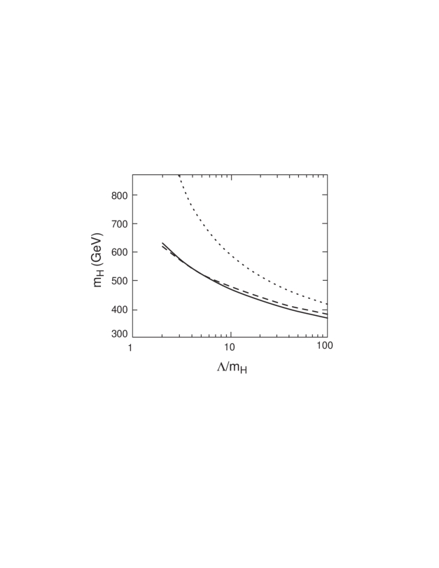
Figure 2: Upper bound on the Higgs boson mass as a function of $\Lambda$/$m_{H}$, where $\Lambda$ is the scale of new physics. The dotted curve is obtained by identifying $\Lambda$ with the Landau pole of $\lambda$ and is given by Eq. (120). The solid curve [93] is the renormalization group improved unitarity bound (124). The dashed curve is the result of a lattice calculation of Ref. [94]. The figure was taken from Ref. [93].

Eqs. (118)-(120) may be interpreted as follows.

• The perturbative “top down” RG flow from $\mu=\mbox{$\Lambda$}$ to the IR value at $\mu=\mbox{$m_{H}$}$, comprising all solutions of Eq.(2) starting from arbitrary perturbatively allowed initial values, $\mbox{$\lambda$}(\mbox{$\Lambda$})/(4\pi)<1$, is attracted towards the IR attractive fixed point $\lambda$=0.

• The IR value $\lambda$($\mu$) becomes the more independent of the initial value $\lambda$($\Lambda$) and the closer to the upper bound (119), the larger the UV initial value $\lambda$($\Lambda$) is chosen (within the framework of perturbation theory). The bound may be interpreted to approximately collect the IR images of all sufficiently large UV initial values.

• The IR coupling $\mbox{$\lambda$}(\mu)$ as well as its upper bound (119) and the triviality bound (120) for the Higgs mass decrease with increasing value of the UV cut-off $\Lambda$.

In the fictitious case of the pure $\phi^{4}$ theory, which as a mathematical toy model need not be subject to any physical UV cut-off $\Lambda$, the limit $\mbox{$\Lambda$}\rightarrow\infty$ can be performed and indeed the full perturbative RG flow is drawn into the IR fixed point value $\lambda$=0  for the renormalized coupling, leading to a trivial non-interacting theory (within the framework of perturbation theory, discussed so far).

In the SM we do, however, expect a physical UV cut-off $\Lambda$ to play the role of the scale above which new physics enters, as expanded on in the Introduction. So, as far as these simple-minded perturbative arguments go, we expect a $\Lambda$ dependent upper bound (120) for the SM Higgs mass which decreases for increasing UV cut-off $\Lambda$. As was first pointed out in Ref. [8], this allows to determine an approximate absolute (perturbative) upper bound for the Higgs mass: on the one hand the triviality bound for the Higgs mass increases with decreasing $\Lambda$; on the other hand the Higgs mass is a physical quantity, which the SM is supposed to describe; so, for consistency, one has to require $\mbox{$m_{H}$}<\mbox{$\Lambda$}$. This implies an absolute upper bound for the Higgs mass close to the region where $m_{H}$ and $\Lambda$ meet.

A more subtle issue is to determine an absolute (perturbative) upper bound for the Higgs mass $m_{H}$ sufficiently much smaller than $\Lambda$, such that the SM physics continues to hold even somewhat above $m_{H}$

• without being too close to violating unitarity [92],[93],

• without running out of the region of validity of perturbation theory and

• without being significantly influenced by the nearby cutoff effects, i.e. by the new physics becoming relevant at energies $O(\mbox{$\Lambda$})$.

These three issues are of course not unrelated. In the following we shall summarize efforts in the recent literature to determine such an absolute bound for $m_{H}$ on a quantitative level for each of these itemized issues within the framework of perturbation theory. All of them apply to the full SM and not only to its Higgs sector, which does, however, not make a significant difference to the issue of an upper Higgs mass bound. They end up with very similar results. As we shall see, these results are also supported in a mellowed form by non-perturbative lattice results in the pure Higgs sector. Altogether rather convincing conclusions can be drawn.

In order to implement the constraint of the unitarity bound, an interesting improvement on the perturbative triviality bound (120) was introduced in Ref. [93]. The UV cut-off $\Lambda$ is identified with the momentum scale where perturbative unitarity is violated, an ansatz which goes back to Ref. [92]. The tightest condition is obtained from the (upper) unitarity bound on $|a_{0}(I=0)|$, where $a_{0}$ is the zeroth partial wave amplidude of the isospin $I=0$ channel in $W_{L}W_{L}\rightarrow W_{L}W_{L}$ scattering. The well known unitarity bound $|Re\,a_{0}(I=0)|\leq 1$ has been tightened to

$$|Re\,a_{0}(I=0)|\leq 1/2$$ (121)

in Ref. [94]. In the limit of center of mass energy $\gg\mbox{$m_{H}$}$ the tree level expression for $a_{0}(I=0)$ is

$$a_{0}(I=0)=-5\mbox{$\lambda$}/(16\pi);$$ (122)

thus, one may conclude that the maximally allowed value for $\lambda$($\Lambda$) is

$$\mbox{$\lambda$}(\mbox{$\Lambda$})\leq\frac{8\pi}{5}.$$ (123)

Feeding this inequality into the one-loop relation (118) leads to the improved perturbative one-loop triviality bound

$$\mbox{$m_{H}$}\leq\frac{2\pi/\sqrt{3}}{\sqrt{\ln\frac{\mbox{$\Lambda$}}{\mbox{$m_{H}$}}+\frac{{\displaystyle 5\pi}}{{\displaystyle 12}}}}\;v$$ (124)

with $v=(\sqrt{2}G_{F})^{-1/2}$. This so-called renormalization group improved unitarity bound is clearly tighter than the bound (120); it is exhibited as solid curve in Fig. 2. One can read off that an absolute upper Higgs mass bound, required to be a factor two below the cut-off $\Lambda$, is reached for $\mbox{$m_{H}$}\simeq 600\mbox{$\,{{\rm GeV}}$}$; applicability up to $\mbox{$\Lambda$}=2\,{\rm TeV}$ requires a bound $\mbox{$m_{H}$}\mbox{\,\raisebox{1.29167pt}{$<$}$\!\!\!\!\!$\raisebox{-3.87495pt}{$\sim$}\,}530\mbox{$\,{{\rm GeV}}$}$.

A recent quantitative analysis of the breakdown of perturbation theory for a large Higgs mass was performed in Ref. [95]. The $\mu$ dependence within different renormalization schemes (the $\overline{{\rm MS}}$ scheme and the on mass shell scheme) is investigated in three physical observables which are known at two-loop level. The criterion for validity of perturbation theory is that the dependence on the renormalization scale $\mu$ as well as on the scheme should diminish order by order in $\lambda$. The conclusion [95] is that perturbation theory breaks down for $m_{H}$=O(700$\,{{\rm GeV}}$) and $m_{H}$ must be $\mbox{$m_{H}$}\mbox{\,\raisebox{1.29167pt}{$<$}$\!\!\!\!\!$\raisebox{-3.87495pt}{$\sim$}\,}{\rm O}(400\mbox{$\,{{\rm GeV}}$})$ for perturbatively calculated cross sections to be trustworthy up to center of mass energies of O(2 TeV).

The effects of a nearby cut-off $\Lambda$ in case of a large Higgs mass in terms of corrections of the order of $m_{H}$/$\Lambda$ have been studied in Ref. [96]. The starting point is the contribution of a virtual Higgs particle in the one-loop vacuum polarization diagrams of weak gauge bosons

$$\Pi_{ij}^{\mu\nu}=-ig^{\mu\nu}(A_{ij}+q^{2}F_{ij}(q^{2}))+q^{\mu}q^{\nu}\ {\rm terms},$$ (125)

where $i$ and $j$ stand for $W^{\pm},\ Z,\,\gamma$. At $q^{2}\leq m_{Z}^{2}$ only $A_{ij}$ and the $F_{ij}(0)$ are retained, moreover $A_{\gamma\gamma}=A_{\gamma Z}=0$ as required from the Ward identities, so that the loop corrections are contained in the six quantities $A_{WW},\ A_{ZZ},\ F_{WW},\ F_{ZZ},\ F_{\gamma Z},\,F_{\gamma\gamma}$. Through renormalization three independent combinations enter the definition of $\alpha,\ G_{F},\ m_{Z}$ and there remain three finite and scheme independent parameters, two of which show a logarithmic dependence on the Higgs mass

$$\epsilon_{1} = \frac{A_{ZZ}}{m_{Z}^{2}}-\frac{A_{WW}}{m_{W}^{2}}=\frac{3}{4}\frac{G_{F}\,\mbox{$m_{t}$}^{2}}{2\sqrt{2}\pi^{2}}+\frac{3}{4}\frac{G_{F}\,m_{W}^{2}}{2\sqrt{2}\pi^{2}}\tan^{2}\theta_{W}\ln(\frac{m_{W}^{2}}{\mbox{$m_{H}$}^{2}}),$$

$$\epsilon_{3} = \cot\theta_{W}F_{30}=\frac{1}{6}\frac{G_{F}\,m_{W}^{2}}{2\sqrt{2}\pi^{2}}\log(\frac{m_{W}^{2}}{\mbox{$m_{t}$}^{2}})-\frac{1}{12}\frac{G_{F}\,m_{W}^{2}}{2\sqrt{2}\pi^{2}}\ln(\frac{m_{W}^{2}}{\mbox{$m_{H}$}^{2}}),$$ (126)

where indices 3 and 0 stand for $W_{3}=\cos\theta_{W}\,Z+\sin\theta_{W}\,\gamma,\ W_{0}=\cos\theta_{W}\,\gamma-\sin\theta_{W}\,Z$ and $\theta_{W}$ is the Weinberg angle. These two quantities are chosen as probes for the sensitivity to a cut-off $\Lambda$.

The $m_{H}$ dependent cut-off scale $\Lambda$, at which new physics is expected, is extracted [96] from the inequality (120) by replacing $m_{H}$ in the logarithm on the right hand side by $v/\sqrt{2}$ and assuming $m_{H}$ on the left hand side to reach its maximal value

$$\mbox{$\Lambda$}=\frac{v}{\sqrt{2}}\,\exp\left(\frac{8\pi^{2}(v/\sqrt{2})^{2}}{3\mbox{$m_{H}$}^{2}}\right).$$ (127)

When a theory becomes sensitive to cut-off effects, it also becomes regularization scheme dependent. The idea [96] is now to simulate the effects of new physics at the $m_{H}$ dependent cut-off $\Lambda$ by calculating the quantities $\epsilon_{1}$ and $\epsilon_{3}$ in three different regularization schemes, i) by introducing a cut-off as an upper limit for the momentum integration, ii) by employing the exponential representation of euclidean propagators and ii) the Pauli-Villars regularization. In all cases the relevant dimensionful cut-off parameter is replaced by Eq. (127). Results for the $m_{H}$ dependence of $\epsilon_{1}$ and $\epsilon_{3}$ in the different schemes, together with the result (126), valid for $\mbox{$\Lambda$}\rightarrow\infty$, are shown in Fig. 3 [96]. In both cases the four curves split at a Higgs mass higher than O(500$\,{{\rm GeV}}$) due to regularization scheme dependent contributions of order $m_{H}$/$\Lambda$ and one cannot trust the predictions of the SM any more.

$\epsilon_{1}$	$\epsilon_{3}$

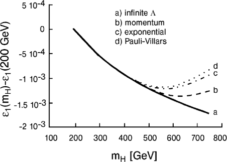
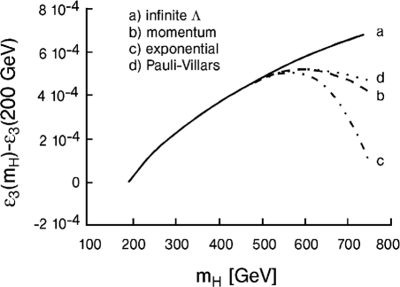
Figure 3: Higgs boson mass dependence of the two quantities $\epsilon_{1}$ and $\epsilon_{3}$. The four curves represent the value at infinite cut-off and with finite cut-off corrections in the three regularization schemes analyzed. The figure was taken from Ref. [96].

In summary, different sources within the framework of perturbation theory come to the conclusion that the SM calculations as functions of increasing Higgs mass are trustworthy up to the upper bound

$$\mbox{$m_{H}$}\simeq{\rm O}(500\mbox{$\,{{\rm GeV}}$}).$$ (128)

The harder part of the proof of triviality and its implications for a triviality bound for the SM Higgs mass is to continue it into the region of large couplings, $\mbox{$\lambda$}(\mbox{$\Lambda$})/(4\pi)\mbox{\,\raisebox{1.29167pt}{$>$}$\!\!\!\!\!$\raisebox{-3.87495pt}{$\sim$}}\,1$, where perturbation theory breaks down. In the early days close to rigorous proofs of triviality of the one-component $\phi^{4}$ theory [97] and of the large $N$ limit of the N-component theory [98] were given. Meanwhile, the dominant tool is lattice $\phi^{4}$ theory with the inverse lattice spacing playing the role of the cut-off $\Lambda$, i.e. of the scale of new physics. Starting with Refs. [99], [8], [100], the triviality of the scalar sector of the SM and therefore the need to retain a finite UV cutoff $\Lambda$ has meanwhile been established for some time by analytical and numerical lattice calculations [101], [94], [102]. The calculations are based on a representative class of lattice actions, all of which respect the property of reflection positivity, the property in this Euclidean formulation which corresponds to unitarity in Minkowski space. A lattice triviality bound [94] is shown in Fig. 2 [93]. It is in surprisingly good agreement with the renormalization group improved unitarity bound. A conservative conclusion [103] on an absolute triviality bound for the Higgs mass as obtained from a representative class of lattice actions is the following: the SM will describe physics to an accuracy of a few percent up to energies of the order 2 to 4 times the Higgs mass $m_{H}$ only if

$$\mbox{$m_{H}$}\leq 710\pm 60\,\mbox{$\,{{\rm GeV}}$}.$$ (129)

Altogether, the non-perturbative lattice calculations confirm the results obtained within the perturbative framework and even relax the absolute upper bound on $m_{H}$ somewhat.

The Higgs mass triviality bound is a weak function of the top Yukawa coupling, resp. the top mass. This dependence will be explicitely discussed in Sects. 4.2, 4.4 and 6.2.

4.2 The Higgs-Top Sector of the SM
– a first IR Fixed Line and a First Vacuum Stability Bound

In the next step towards the SM a reduction to two coupling parameters, the Higgs selfcoupling $\lambda$ and the top Yukawa coupling $g_{t}$ is considered,

$$\mbox{$\lambda$}\neq 0,\;\mbox{$g_{t}$}\neq 0\hskip 56.9055pt{\rm with\ all\ the\ other\ couplings}\,=0.$$ (130)

This reduced system is of interest since even though it is still “trivial” with respect to both couplings, $\lambda$ and $g_{t}$, it exhibits - as we shall see - a non-trivial IR fixed line in the plane of the two couplings which is more strongly IR attractive than the fixed point and it can still be solved analytically. This fixed line turns out to be the dynamical origin i) for the triviality bound, the upper bound of the Higgs mass, which in this two coupling framework becomes a weak function of the top mass as well as ii) for the lowest order vacuum stability bound, the lower bound on the Higgs mass again being a function of the top mass. Furthermore important features find again support by non-perturbative lattice calculations in this $\lambda$-$g_{t}$-framework.

The corresponding RG equations (59) and (62) reduce in one-loop order to

$$\frac{{\rm d}\,\mbox{$g_{t}^{2}$}}{{\rm d}\,t} = \frac{9}{16\pi^{2}}g_{t}^{4}$$ (131)

$$\frac{{\rm d}\,\mbox{$\lambda$}}{{\rm d}\,t} = \frac{6}{16\pi^{2}}(4\mbox{$\lambda$}^{2}+2\mbox{$\lambda$}\mbox{$g_{t}^{2}$}-\mbox{$g_{t}$}^{4}).$$ (132)

This is a coupled system of differential equations. A first observation is that it exhibits a common

$${\rm IR\ attractive\ trivial\ fixed\ point\ at}\hskip 28.45274pt\mbox{$\lambda$}=0,\,\mbox{$g_{t}$}=0.$$ (133)

If the variable

$$R=\frac{\mbox{$\lambda$}}{\mbox{$g_{t}^{2}$}}$$ (134)

is introduced, the system of RG equations (131), (132) may be rewritten in a decoupled form with nested solutions $\mbox{$g_{t}$}=\mbox{$g_{t}$}(\mu)$ and $R=R(\mbox{$g_{t}$}(\mu))$

$$\frac{{\rm d}\,\mbox{$g_{t}^{2}$}}{{\rm d}\,t} = \frac{9}{16\pi^{2}}g_{t}^{4}$$ (135)

$$\mbox{$g_{t}^{2}$}\frac{{\rm d}\,R}{{\rm d}\,\mbox{$g_{t}^{2}$}} = \frac{1}{3}(8R^{2}+R-2).$$ (136)

The right hand side of the differential equation (136) has two zeroes

$$R=\overline{R}=\frac{1}{16}(\sqrt{65}-1),\hskip 14.22636ptR=\overline{\overline{R}}=\frac{1}{16}(-\sqrt{65}-1).$$ (137)

The positive zero $\overline{R}$ is [40] an

$${\rm IR\ attractive\ fixed\ point\ in\ the\ variable}\,\;R{\rm\,\;at}\hskip 14.22636ptR=\overline{R}=\frac{1}{16}(\sqrt{65}-1)\simeq 0.441.$$ (138)

An analogous IR fixed point had already been pointed out in an earlier publication [32] in application to a fourth heavy fermion generation. Here we meet for the first time a fixed point in the ratio of couplings $R=\mbox{$\lambda$}/\mbox{$g_{t}^{2}$}$, which has also been termed (in a context to be discussed in the next subsection) a “quasi-fixed point” [30]. In the $\lambda$-$g_{t}$-plane it corresponds to a fixed line, which is linear and goes through the origin

$$\mbox{$\lambda$}=\frac{1}{16}(\sqrt{65}-1)\,\mbox{$g_{t}^{2}$}.$$ (139)

It has the property that the solution stays on the fixed line for all values of $\mu$, once its initial value is chosen on it. Its analytical form is independent of initial values $\Lambda$, $\mbox{$g_{t}$}_{0}$ and $\mbox{$\lambda$}_{0}$. It is the solution of the RGE which is defined by the boundary condition that the ratio $\lambda$/$g_{t}^{2}$ has a finite non-zero value in the limit $\mbox{$\lambda$},\,\mbox{$g_{t}^{2}$}\rightarrow\infty$; as announced earlier, this boundary condition refers to a limit which leads outside the region of validity of perturbation theory; nevertheless the IR attraction of this IR fixed line applies to the RG flow in the perturbative region.

Going beyond Ref. [40], one can determine analytically the way in which the “top-down” RG flow approaches the IR fixed line and finally the IR fixed point from the analytical solution to the system of differential equations (136)

$$\mbox{$g_{t}^{2}$}(t) = \frac{g_{t0}^{2}}{1+\frac{{\displaystyle 9}}{{\displaystyle 16\pi^{2}}}g_{t0}^{2}\ln\frac{\mbox{$\Lambda$}}{{\displaystyle\mu}}}$$ (140)

$$R(\mbox{$g_{t}^{2}$}) = \frac{\mbox{$\lambda$}(\mbox{$g_{t}^{2}$})}{\mbox{$g_{t}^{2}$}}=\frac{\overline{R}-{\displaystyle\frac{R_{0}-\overline{R}}{R_{0}-\overline{\overline{R}}}}\;\overline{\overline{R}}\;({\displaystyle{\frac{\mbox{$g_{t}^{2}$}}{g_{t0}^{2}}}})^{\sqrt{65}/3}}{1-{\displaystyle\frac{R_{0}-\overline{R}}{R_{0}-\overline{\overline{R}}}}\;({\displaystyle\frac{\mbox{$g_{t}^{2}$}}{g_{t0}^{2}}})^{\sqrt{65}/3}}.$$ (141)

for arbitrary (perturbatively allowed) initial values

$$g_{t0}=\mbox{$g_{t}$}(\mbox{$\Lambda$}),\;\;\;R_{0}=\frac{\lambda_{0}}{g_{t0}^{2}}=\frac{\mbox{$\lambda$}(\mbox{$\Lambda$})}{\mbox{$g_{t}^{2}$}(\mbox{$\Lambda$})}.$$ (142)

Evolving from the UV to the IR, $\mbox{$g_{t}$}(\mu)$ indeed approaches 0 and correspondingly the RG flow approaches the value $R=\overline{R}$, i.e. the IR fixed line. A measure for the strength of IR attraction towards the fixed line is the exponent in $(\mbox{$g_{t}^{2}$}/g_{t0}^{2})^{\sqrt{65}/3}$ which is large, $\sqrt{65}/3\simeq 2.69$. So, the RG flow is roughly as follows: first towards the IR fixed line and then close to it or along it towards the IR fixed point (133).

The IR attractive line $\mbox{$\lambda$}=((\sqrt{65}-1)/16)\,\mbox{$g_{t}^{2}$}$ is the dynamical origin for the triviality bound as well as for the vacuum stability bound. The first important observation is that no solution of the considered RGE can cross the IR fixed line. The line is the lower bound for all solutions starting the top-down evolution from an initial value above it and the upper bound for all solutions starting the evolution from an initial value below it. The solutions starting from initial values sufficiently closely above or below the line will end up on the line. The IR images of the solutions starting from the largest possible initial value of the Higgs self coupling $\lambda$ allowed by perturbation theory will constitute the upper, i.e. triviality bound for the IR values; according to Sect. 2.6 the IR images of the lowest possible initial values of $\lambda$, which are $\mbox{$\lambda$}_{0}$=0, constitute the lower, i.e. vacuum stability bound in these lowest order considerations. Given a finite evolution path from some initial scale $\mu=\mbox{$\Lambda$}$ to the IR scale, these bounds will be at some finite difference from the IR fixed line, their position strongly depending on $\Lambda$; they will be the closer to the line the larger the value of $\Lambda$. For $\mbox{$\Lambda$}\rightarrow\infty$, which is of mathematical interest only, the RG flow will first contract towards the IR fixed line and then towards the IR fixed point $\lambda$=0, $g_{t}^{2}$=0. These lowest order bounds may be translated into lowest order Higgs mass bounds in terms of the top mass in the Higgs-top mass plane, using the lowest order relations $\mbox{$m_{H}$}=\sqrt{2\mbox{$\lambda$}(\mu=\mbox{$m_{H}$})}v$ and $\mbox{$m_{t}$}=(v/\sqrt{2})\mbox{$g_{t}$}(\mu=\mbox{$m_{t}$})$. The analytical formula for the $g_{t}^{2}$ dependence of the triviality bound may be obtained from the $\mbox{$\lambda$}_{0}\rightarrow\infty$, i.e. $R_{0}\rightarrow\infty$ limit of the general solution (141)

$$R(\mbox{$g_{t}^{2}$})_{\rm triv}=\frac{\mbox{$\lambda$}(\mbox{$g_{t}^{2}$})}{\mbox{$g_{t}^{2}$}}_{\rm triv}=\frac{\overline{R}-\overline{\overline{R}}({\displaystyle{\frac{\mbox{$g_{t}^{2}$}}{g_{t0}^{2}}}})^{\sqrt{65}/3}}{1-({\displaystyle\frac{\mbox{$g_{t}^{2}$}}{g_{t0}^{2}}})^{\sqrt{65}/3}},$$ (143)

the one for the lowest order vacuum stability bound from the solution (141) with initial value $\mbox{$\lambda$}_{0}=0$, i.e. $R_{0}=0$,

$$R(\mbox{$g_{t}^{2}$})_{\rm vac.stab.}=\frac{\mbox{$\lambda$}(\mbox{$g_{t}^{2}$})}{\mbox{$g_{t}^{2}$}}_{\rm vac.stab.}=\frac{\overline{R}\left(1-({\displaystyle{\frac{\mbox{$g_{t}^{2}$}}{g_{t0}^{2}}}})^{\sqrt{65}/3}\right)}{1-\frac{\overline{R}}{\overline{\overline{R}}}({\displaystyle\frac{\mbox{$g_{t}^{2}$}}{g_{t0}^{2}}})^{\sqrt{65}/3}}.$$ (144)

The corresponding figure in Table 2 shows the $\lambda$-$g_{t}^{2}$-plane with the trivial IR attractive fixed point (133) indicated as diamond, the IR attractive fixed line (139) drawn as fat line and the triviality upper and the vacuum stability lower bounds for four values of $\Lambda$, $\mbox{$\Lambda$}=10^{4},\;10^{6},\;10^{10},$ $10^{15}\mbox{$\,{{\rm GeV}}$}$, drawn as thin lines, which cut out wedgeformed allowed regions which decrease for increasing $\Lambda$. A thorough discussion including figures, more quantitative information about the degree of IR attraction as well as proper reference to the literature will be given in Subsect. 4.4, where the inclusion of the strong gauge coupling leads to a more realistic situation.

a)	b)

Figure 4: a) lattice results [105] for the upper and lower bounds on $g_{R}$ (corresponding to 6$\lambda$) as a function of $G^{2}_{R\psi}$ (corresponding to $g_{t}^{2}/2$) together with the one-loop estimates for scale ratios $\mbox{$\Lambda$}/\mbox{$m_{H}$}=3$ (solid curve) and $\mbox{$\Lambda$}/\mbox{$m_{H}$}=4$ (dotted curve). The open symbols denote the lower bound, the full symbols the upper bound; the triangles represent the $6^{3}\cdot 12$ lattice results, the squares the $8^{3}\cdot 16$ lattice results. b) The mass ratio $\mu_{R\psi}/m_{R\sigma}$ (corresponding to $\mbox{$m_{H}$}/m_{t}$) as a function of $G_{R\psi}$ (corresponding to $g_{t}/\sqrt{2}$) in comparison with one-loop perturbative estimates for $m_{R\sigma}=0.75$ (dotted curve), $m_{R\sigma}=1$ (full curve) and $m_{R\sigma}=1.25$ (dashed curve). The figures were taken from Ref. [105].

Again it is of interest to go beyond perturbation theory and look for confirmation to non-perturbative lattice calculations in the Higgs-fermion sector. In Refs. [104],[105] non- perturbative results for the triviality bound as well as the vacuum stability bound have been obtained. The investigations are based on a lattice action which is the sum of an $O(4)$ ($\simeq SU(2)_{L}\times SU(2)_{R}$) scalar part and a fermionic part with chiral $SU(2)_{L}\times SU(2)_{R}$ symmetry involving a heavy fermion doublet without mass splitting, supplemented by a corresponding mirror fermion doublet in order to overcome the notorious fermion doubler problem accompanying regularization on the lattice. Mass mixing between the doublets is arranged such as to exactly decouple [106] the mirror fermions from the physical spectrum. The calculations are performed in the physically relevant broken symmetry phase. The triviality bound results from bare Higgs selfcoupling $\mbox{$\lambda$}=\infty$, the vacuum stability bound from $\mbox{$\lambda$}=10^{-6}$.

The results are shown in Fig. 4a) [105], where the renormalized Higgs selfcoupling $g_{R}$ corresponds to the IR coupling 6$\lambda$ in our nomenclature and the renormalized Yukawa coupling $G_{R\psi}$ is to be identified with the IR top Yukawa coupling $\mbox{$g_{t}$}/\sqrt{2}$. For comparison the perturbative one-loop results for $\Lambda$=3$m_{H}$ and $\Lambda$=4$m_{H}$ are shown. As in the pure Higgs case, the lattice calculations confirm the one-loop perturbative bounds; the lattice bounds are “absolute bounds” in the same sense as the $\Phi^{4}$ lattice bound (129) for the Higgs mass: they allow the physics of the Higgs fermion sector to continue to be valid up to scales $\Lambda$ of the order of three to four times the Higgs mass.

An interesting result is the right-most point in Fig. 4a) [105] with large error bars at largest values of the two couplings. It implies a lattice “absolute” upper bound (129) for the fermion mass

$$m_{f}\mbox{\,\raisebox{1.29167pt}{$<$}$\!\!\!\!\!$\raisebox{-3.87495pt}{$\sim$}\,}O(600\pm 80\mbox{$\,{{\rm GeV}}$}),$$ (145)

which however leaves only a safety margin for the model up to a cut-off $\mbox{$\Lambda$}\simeq 1.9\,\rm m_{f}$. The upper limit is provided by the requirement of reflection positivity, the Euclidean analogue of unitarity in Minkowski space. The rightmost point in Fig. 4a) [105] is of further interest, since it allows to trace the IR fixed line in the $\lambda$-$g_{t}^{2}$ plane, resp. the IR fixed point in the ratio R=$\lambda$/$g_{t}^{2}$, Eq. (138), in the lattice data. In Fig. 4b) [105] the lattice bounds tend towards a ratio for the fermion mass divided by the Higgs mass $\mu_{R\psi}/m_{R\sigma}=0.76$ which corresponds to the IR fixed point position $R=\mbox{$\lambda$}/\mbox{$g_{t}^{2}$}=(\sqrt{65}-1)/16\simeq 0.441$, determined in Eq. (138) .Thus all features of one-loop perturbation theory in the Higgs-top sector are supported by non-perturbative lattice calculations.

4.3 The Top-$g_{3}$ Sector of the SM and MSSM
– a Non-Trivial IR Fixed Point

As a first step towards including the strong gauge coupling $g_{3}$ the subset of the two couplings

$$\mbox{$g_{t}$},\ \mbox{$g_{3}$}\neq 0,\ {\rm in\ the\ SM}\ {\rm resp.}\ \mbox{$h_{t}$},\ \mbox{$g_{3}$}\neq 0,\ {\rm in\ the\ MSSM}\ \hskip 22.76219pt{\rm with\ all\ the\ other\ couplings}=0$$ (146)

is treated. A first non-trivial IR fixed point appears in the variable $\rho_{t}$=$g_{t}^{2}$/$g_{3}^{2}$ in the SM and in the corresponding variable $\rho_{t}$=$h_{t}^{2}$/$g_{3}^{2}$ in the MSSM. Let us point out already here that this IR fixed point will turn out to be at the heart of the quantum effects, as encoded in the RGE, which will finally lead to an IR attractive top mass value

$$m_{t}^{{\rm pole}} \approx 215\mbox{$\,{{\rm GeV}}$}\ {\rm in\ the\ SM}$$ (147)

$$m_{t}^{{\rm pole}} \approx O(190-200)\mbox{$\,{{\rm GeV}}$}\sin\beta\ {\rm in\ the\ MSSM}$$ (148)

after inclusion of further couplings, in particular of the electroweak gauge couplings, of the two-loop contributions in the RGE and of the radiative corrections leading to the pole mass.

In case of the SM the fixed point was first pointed out in this form to be discussed next by Pendleton and Ross [30]; their paper may justly be considered to be the primer for all following investigations into IR fixed points, lines, surfaces in the space of ratios of variables. Earlier references to an IR fixed point were made in Refs. [29]. Subsequent important results concerning the IR fixed point were obtained in Ref. [31], also to be discussed below, and in Refs. [32]-[37], concentrating mainly on the issues of new heavy fermion generations or of two Higgs doublets. The Pendleton-Ross IR fixed point was rediscovered and expanded on in Refs. [38] and [39] as a renormalization group invariant solution in the framework of reduction of parameters, to be reviewed in Sect. 8. Later developments were made in Refs. [40]-[42], [48].

The corresponding IR fixed point in the MSSM was discussed in Refs. [43]-[48]. An explosive development [49]-[65] focused on the interrelated issues of tau-bottom(-top) Yukawa coupling unification in supersymmetric grand unification and of an IR fixed top mass value, Eq. (148), to be reviewed in Sect. 7.

The introduction of the ratio of coupling squares

$$\mbox{$\rho_{t}$}=\frac{\mbox{$g_{t}^{2}$}}{\mbox{$g_{3}^{2}$}}{\rm\ in\ the\ SM}\;\;\;\;{\rm and}\;\;\;\;\mbox{$\rho_{t}$}=\frac{\mbox{$h_{t}^{2}$}}{\mbox{$g_{3}^{2}$}}{\rm\ in\ the\ MSSM},\;\;\;\;\;\;{\rm respectively,}$$ (149)

in Refs. [30]-[42] and [43]-[48] leads to the respective RG equations in $\rho_{t}$

$${\rm SM}$$

(150)

in terms of the variable $g_{3}^{2}$. Following Refs. [31]-[39],[42] for the SM and Ref. [47] for the MSSM, the general solutions of the RGE (150) for $\rho_{t}$ and that for $g_{3}$, are

$${\rm SM}$$

,

(151)

where

$$g_{30}^{2} = \mbox{$g_{3}^{2}$}(\mbox{$\Lambda$}),$$ (152)

$$\rho_{t0} = \mbox{$\rho_{t}$}(\mbox{$g_{3}^{2}$}(\mbox{$\Lambda$})).$$ (153)

From Eqs. (150) and (151) the following important analytical results i) about an exact IR fixed point, first discovered by Ref.[30] within the SM and ii) an effective IR fixed point, first discovered by Ref. [31] within the SM, may be read off. Further references were given already in the introduction of this subsection.

• The differential equation for $\rho_{t}$($g_{3}^{2}$) has an exact fixed point at

  $${\rm SM}$$

  (154)

  This fixed point corresponds to the special solution of the RGE defined by the boundary condition that $\rho_{t}$ approaches a finite value ($\not=0$) in the limit $\mbox{$g_{3}^{2}$}\rightarrow 0$. This special solution remains in the fixed point, once it has started in this fixed point value, irrespective of the evolution of $g_{3}^{2}$  i.e. in particular of the choice of initial values $\Lambda$, $g_{30}^{2}$  and of $g_{t0}^{2}$. In the $g_{t}^{2}$-$g_{3}^{2}$ plane, resp. in the $h_{t}^{2}$-$g_{3}^{2}$ plane, this fixed point in $\rho_{t}$ translates into a fixed line (physicists’ terminology) or invariant line (mathematicians’ terminology [89]), $\mbox{$g_{t}^{2}$}=2/9\mbox{$g_{3}^{2}$}$ and $\mbox{$h_{t}^{2}$}=7/18\mbox{$g_{3}^{2}$}$, respectively. This implies that once the initial value is chosen on this line, the solution evolves along this line; again the location of this line is independent of the initial values $\Lambda$, $g_{30}^{2}$ and $g_{t0}^{2}$. Since, however, as anticipated in the introduction of this Sect. 4, all further IR fixed points, lines and surfaces will appear in spaces of ratios of variables it is more economical to stick to the ratio $\rho_{t}$ as new variable in the following.

• The IR fixed point (154) in $\rho_{t}$ is IR attractive, i.e. it attracts all solutions starting from arbitrary (perturbatively allowed) initial values $g_{30}^{2}$, $\mbox{$\rho_{t0}$}>0$ at $\mu=\mbox{$\Lambda$}$ for arbitrary $\Lambda$, in short the (perturbative) “top-down” RG flow, towards it. However, as has been pointed out in Ref. [31], in case of the SM this attraction is exceedingly weak, like $(\mbox{$g_{3}^{2}$}/\mbox{$g_{30}^{2}$})^{-1/7}$, where the logarithmic evolution of $g_{3}^{2}$ is damped by the prohibitively small exponent, -1/7. This is, however, not the case [47] in the MSSM, where the corresponding exponent is -7/9, i.e. reasonably large. In any case, however, the full RG flow reaches the fixed point (154) only in the limit $\mbox{$g_{3}$}\rightarrow\infty$ which is outside of the range of validity of perturbation theory and of mathematical interest only.

• Of high interest is the upper bound [6], [7], [31], [32], [10], [40] for the variable $\rho_{t}$. As has been worked out analytically in Ref. [31], an almost $\rho_{t0}$ independent upper bound for $\rho_{t}$ is approached for sufficiently large UV initial values $\rho_{t0}$. Neglectingin Eqs. (151) 1/$\rho_{t0}$ with respect to 2/9 and 7/18, respectively, allows to read off the $\rho_{t0}$ independent upper bound, which could also be termed a triviality bound for the variable $\rho_{t}$

  $${\rm SM}$$

  .

  (155)

  Evaluated at the IR scale, this upper bound is roughly the IR image of all sufficiently large UV initial values $\rho_{t0}$ for $\rho_{t}$. In the limits $\mbox{$\Lambda$}\rightarrow\infty$ or $\mbox{$g_{3}$}\rightarrow\infty$, which of course both are physically not accessible, the upper bound tends towards the Pendleton-Ross fixed point. Thus, as in the case of the triviality bound for the Higgs selfcoupling $\lambda$, it is the finite length of the RG evolution path from the UV to the IR which is responsible for the finite gap between the upper bound (155) and the IR fixed point (154). The upper bound decreases for increasing value of the UV cut-off $\Lambda$.

  Ref. [31] went even further and very intuitively reinterpreted the upper bound (155) in case of the SM as an effective intermediate IR fixed point for solutions with large UV initial values $\rho_{t0}$ or $g_{t0}$ as follows. On the one hand, considering $\frac{1}{7}\ln(\mbox{$g_{3}^{2}$}/\mbox{$g_{30}^{2}$})$ as small expansion parameter, the bound (155) may be rewritten approximately as

  $$\mbox{$\rho_{t}$}(\mbox{$g_{3}^{2}$})_{\rm upper\ bound} \approx \frac{2}{9}\frac{7}{\ln\frac{\mbox{$g_{3}^{2}$}}{\mbox{$g_{30}^{2}$}}}\left(1+O(\frac{1}{7}\ln\frac{\mbox{$g_{3}^{2}$}}{\mbox{$g_{30}^{2}$}})\right),\ \ {\rm i.e.}$$

  $$\mbox{$g_{t}^{2}$}(\mbox{$g_{3}^{2}$})_{\rm upper\ bound} \approx \frac{14}{9}\frac{\mbox{$g_{3}^{2}$}}{\ln\frac{\mbox{$g_{3}^{2}$}}{\mbox{$g_{30}^{2}$}}}.$$ (156)

  On the other hand, in going back to the RGE for $g_{t}^{2}$,

  $$\frac{{\rm d}\,\mbox{$g_{t}^{2}$}}{{\rm d}\,t}=\frac{\mbox{$g_{t}^{2}$}}{8\pi^{2}}\,\left(\frac{9}{2}\mbox{$g_{t}^{2}$}-8\mbox{$g_{3}^{2}$}\right),$$ (157)

  Hill points out [31] that for large initial values $\mbox{$g_{t0}^{2}$}\gg\mbox{$g_{30}^{2}$}$ in the vicinity of the UV scale the running of $g_{t}^{2}$ is driven by the term $\frac{9}{2}\mbox{$g_{t}^{2}$}$ in the bracket, which justifies to replace $8\mbox{$g_{3}^{2}$}$ in the bracket by some constant average value $8\overline{\mbox{$g_{3}^{2}$}}$. In running with $\mu$ towards the $\rho_{t0}$ independent upper bound in the IR region, a transient slowing down in the running of $g_{t}^{2}$ is expected in the vicinity of the value of $\mu$ where the bracket and consequently ${\rm d}\,\mbox{$g_{t}^{2}$}/{\rm d}\,t$ become zero for

  $$\frac{9}{2}\mbox{$g_{t}^{2}$}\approx 8\overline{\mbox{$g_{3}^{2}$}}.$$ (158)

  Since this slowing down is expected to happen in the vicinity of the upper bound (155), one may identify [31]

  $$\overline{\mbox{$g_{3}^{2}$}}\approx\frac{7}{8}\frac{\mbox{$g_{3}^{2}$}(\mu)}{\ln\frac{\mbox{$g_{3}^{2}$}(\mu)}{\mbox{$g_{30}^{2}$}}}.$$ (159)

  In the supersymmetric case, the analogon of the transient slowing down condition (158) is

  $$6\mbox{$h_{t}^{2}$}\approx\frac{16}{3}\overline{\mbox{$g_{3}^{2}$}},$$ (160)

  which was pointed out in Ref. [45]. As was also stressed in Ref. [31], the effective intermediate IR fixed point is not a genuine fixed point, since its position depends on the UV cut-off $\Lambda$ as well as on the initial value $g_{30}^{2}$ and it is not attractive for smaller initial values $\rho_{t0}$.

  As the Hill intermediate effective fixed point appears as an approximate interpretation of the upper bound (155), the notions of an upper bound and of an effective fixed point have been frequently treated as synonymous in the literature. In the following we also shall repeatedly prefer the notion of “Hill effective fixed point” over the notion “upper bound”, since it reflects more directly the very strong IR attraction of the bound for solutions with large $\rho_{t0}$ as well as its independence of the (large) initial value $\rho_{t0}$.

• A very important point to realize is that this strong attraction towards the upper bound, resp. the Hill effective fixed point, implies a strong effect of effacing the memory of the details of the UV physics in the IR physics: any theory at some high UV scale $\Lambda$, which supplies for some dynamical reason sufficiently large UV initial values for the top Yukawa coupling, will end up in the upper bound, resp. in the Hill effective fixed point in the IR region; the only memory retained is the scale $\Lambda$ at which new physics is present. A very good example is (as has also been worked out by the authors) the appealing scheme running under the name of top condensation [107], e.g. reviewed in Ref. [108]. At some high scale $\Lambda$ a new physics sector provides the force for the condensation of top-antitop pairs thus providing a dynamical mechanism for the spontaneous electroweak symmetry breaking and a composite Higgs boson. The RG evolution of the naturally large UV initial values for the top Yukawa couplings largely effaces the details of the UV theory and ends up in the IR region in the $\Lambda$ dependent top Yukawa values of the IR upper bound, i.e. the Hill effective fixed point.

The final aim is of course to translate the fixed point position in the variable $\rho_{t}$ into the corresponding values for the top mass, which is in lowest order

$$m_{t} = \sqrt{2/9}\mbox{$g_{3}$}(\mu=\mbox{$m_{t}$})v/\sqrt{2}\approx 95\mbox{$\,{{\rm GeV}}$}\ \ {\rm in\ the\ SM},$$ (161)

$$m_{t} = \sqrt{7/18}\mbox{$g_{3}$}(\mu=\mbox{$m_{t}$})v/\sqrt{2}\sin\beta\approx 126\mbox{$\,{{\rm GeV}}$}\sin\beta\ \ {\rm in\ the\ MSSM}$$ (162)

In the approximation considered so far, already a comparatively large top mass results. Also the upper bounds on the top mass corresponding to the Hill effective fixed point may be estimated that way

$$\mbox{$m_{t}$}_{{\rm max}} \approx 570,\,460,\,300,\,230\mbox{$\,{{\rm GeV}}$}\ {\rm resp.\ for}\ \mbox{$\Lambda$}=10^{4},\,10^{6},\,10^{10},\,10^{15}\mbox{$\,{{\rm GeV}}$}\ {\rm in\ the\ SM},$$ (163)

$$\mbox{$m_{t}$}_{{\rm max}} \approx 175\sin\beta\mbox{$\,{{\rm GeV}}$}\ {\rm for}\ \mbox{$\Lambda$}=\mbox{$M_{{\rm GUT}}$}\approx 2\cdot 10^{16}\mbox{$\,{{\rm GeV}}$}\ {\rm in\ the\ MSSM}$$ (164)

Given the approximation, this may be considered as a very convincing step towards physical reality. It shows that at the level of the quantum effects, as encoded in the RGE equations, resides the intrinsic possibility of a heavy top quark, i.e. a top quark much heavier than the other quarks and leptons. In order to get quantitatively reliable results, one has i) to switch back on the electroweak couplings $g_{1}$, $g_{2}$ as well as the Higgs, bottom and tau couplings, ii) use the full two-loop RGE and iii) take into account the radiative corrections allowing to determine the pole mass $m_{t}^{{\rm pole}}$. These “corrections” (in particular the introduction of the electroweak couplings) will turn out to significantly increase the top mass to the values anticipated already in Eq. (148). The corrections will be introduced step by step in the following sections.

4.4 The Higgs-Top-$g_{3}$ Sector of the SM
– a First Non-Trivial Approximation

Now the necessary information has been accumulated to discuss the first approximation to the SM which is non-trivial from the mathematical point of view and qualitatively already informative from the physical point of view. A dynamical source for a heavy Higgs boson arises which is intimately related to the one for the a heavy top quark discussed in the last section.

The three couplings

$$\mbox{$\lambda$},\ \mbox{$g_{t}$},\ \mbox{$g_{3}$}\ \not=0$$ (165)

are considered to be the only non-vanishing ones in the RGE of the SM in this subsection.

As above it is more economical to consider the ratios of couplings

$$\mbox{$\rho_{t}$}=\frac{\mbox{$g_{t}^{2}$}}{\mbox{$g_{3}^{2}$}}\ \ {\rm and}\ \ \mbox{$\rho_{H}$}=\frac{\mbox{$\lambda$}}{\mbox{$g_{3}^{2}$}}$$ (166)

or even

$$\mbox{$\rho_{t}$}=\frac{\mbox{$g_{t}^{2}$}}{\mbox{$g_{3}^{2}$}}\ \ {\rm and}\ \ R=\frac{\mbox{$\rho_{H}$}}{\mbox{$\rho_{t}$}}=\frac{\mbox{$\lambda$}}{\mbox{$g_{t}^{2}$}}.$$ (167)

By rewriting as in the last subsection $g_{3}^{2}$ as function of t, $\rho_{t}$ as function of $g_{3}^{2}$ and finally $\rho_{H}$ or alternatively R as a function of $\rho_{t}$, one ends up with the following system of decoupled differential equations [42]

$${\displaystyle\frac{{\rm d}\,\mbox{$g_{3}^{2}$}}{{\rm d}\,t}} = {\displaystyle-7\frac{g_{3}^{4}}{8\pi^{2}}}$$ (168)

$${\displaystyle-14\mbox{$g_{3}^{2}$}\frac{{\rm d}\,\mbox{$\rho_{t}$}}{{\rm d}\,\mbox{$g_{3}^{2}$}}} = {\displaystyle\mbox{$\rho_{t}$}\left(9\mbox{$\rho_{t}$}-2\right)}$$ (169)

$${\displaystyle\mbox{$\rho_{t}$}\left(9\mbox{$\rho_{t}$}-2\right)\frac{{\rm d}\,\mbox{$\rho_{H}$}}{{\rm d}\,\mbox{$\rho_{t}$}}} = {\displaystyle 24\mbox{$\rho_{H}$}^{2}+(12\mbox{$\rho_{t}$}+14)\mbox{$\rho_{H}$}-6\mbox{$\rho_{t}$}^{2}}$$ (170)

or alternatively [42]

$${\displaystyle\frac{{\rm d}\,\mbox{$g_{3}^{2}$}}{{\rm d}\,t}} = {\displaystyle-7\frac{g_{3}^{4}}{8\pi^{2}}}$$ (171)

$${\displaystyle-14\mbox{$g_{3}^{2}$}\frac{{\rm d}\,\mbox{$\rho_{t}$}}{{\rm d}\,\mbox{$g_{3}^{2}$}}} = {\displaystyle\mbox{$\rho_{t}$}\left(9\mbox{$\rho_{t}$}-2\right)}$$ (172)

$${\displaystyle(9\mbox{$\rho_{t}$}-2)\frac{{\rm d}\,R}{{\rm d}\,\mbox{$\rho_{t}$}}} = {\displaystyle 24R^{2}+(3+\frac{16}{\mbox{$\rho_{t}$}})R-6}.$$ (173)

The system of differential equations for $\rho_{t}$ and $\rho_{H}$  resp. R, has a common IR fixed point first pointed out in Ref. [30] and further analyzed in Refs. [31], [35]-[39], [41], [42].

$$\mbox{$\rho_{t}$}=\frac{2}{9},\hskip 56.9055pt\mbox{$\rho_{H}$}={\displaystyle\frac{\sqrt{689}-25}{72}},\ \ {\rm resp.}\ \ R={\displaystyle\frac{\sqrt{689}-25}{16}}.$$ (174)

Thus, in presence of the gauge coupling $g_{3}$ the nontrivial top fixed point, discussed in the previous subsection, is supplemented by a nontrivial Higgs fixed point. This common fixed point replaces the trivial IR fixed point at $\mbox{$\lambda$}=\mbox{$g_{t}^{2}$}=0$ in absence of $g_{3}$. It is also interesting as a crude approximation to physical reality, since it corresponds within this lowest order perturbation theory to

$$m_{t} = \sqrt{2/9}\mbox{$g_{3}$}(\mu=\mbox{$m_{t}$})v/\sqrt{2}\approx 95\mbox{$\,{{\rm GeV}}$}$$ (175)

$$m_{H} = \sqrt{(\sqrt{689}-25)/72}\mbox{$g_{3}$}(\mu=\mbox{$m_{t}$})\sqrt{2}v\approx 53\mbox{$\,{{\rm GeV}}$}.$$ (176)

Again, the common IR fixed point can be viewed in the presently discussed approximation as a possible dynamical origin for large top quark and Higgs masses! It will eventually lead to mass values

$$m_{t}^{{\rm pole}} \simeq 214\mbox{$\,{{\rm GeV}}$}\ {\rm in\ the\ SM}$$ (177)

$$m_{H}^{{\rm pole}} \simeq 210\mbox{$\,{{\rm GeV}}$},$$ (178)

when all the appropriate corrections are applied in the next sections.

As in the $\lambda$-$g_{t}^{2}$ plane in absence of $g_{3}$, there is again an IR attractive fixed line $\overline{r}_{H}(\mbox{$\rho_{t}$})$ in the $\rho_{t}$-$\rho_{H}$-plane or alternatively $\overline{R}(\mbox{$\rho_{t}$})$ in the $\rho_{t}$-R-plane [42], with prior indications already contained in Refs. [35]-[39],[41]. This fixed line is nonlinear in contradistinction to the one in absence of $g_{3}$. It is the solution of the RGE singled out by the boundary condition of approaching a finite ratio $R=\mbox{$\rho_{H}$}/\mbox{$\rho_{t}$}=\mbox{$\lambda$}/\mbox{$g_{t}^{2}$}$ in the limit $\mbox{$\rho_{t}$},\,\mbox{$\rho_{H}$}\rightarrow\infty$ or $\mbox{$g_{t}^{2}$},\,\mbox{$\lambda$}\rightarrow\infty$. In fact the limit is

$$\overline{\rho}_{H}(\mbox{$\rho_{t}$})\rightarrow\frac{\sqrt{65}-1}{16}\,\mbox{$\rho_{t}$},\ \ \ {\rm resp.}\ \ \ \overline{R}(\mbox{$\rho_{t}$})\rightarrow\frac{\sqrt{65}-1}{16}\ \ {\rm for}\ \ \mbox{$\rho_{t}$}\rightarrow\infty.$$ (179)

Since in this limit the couplings $\lambda$ and $g_{t}^{2}$ are much larger than $g_{3}^{2}$, we are back to the discussion led in Refs. [32], [40] and reported on in Subsect. 4.2. Indeed, this limit is consistently identical with the slope (139) of the IR attractive line in the $\lambda$-$g_{t}^{2}$-plane in absence of the strong gauge coupling $g_{3}$. Now the fixed line is the solution of the RGE interpolating also the trivial fixed point at R=0 at $\rho_{t}$=0, which is now IR repulsive (i.e. UV attractive), the IR attractive fixed point (174) at $\rho_{t}$=2/9 and shows the asymptotic behaviour (179) for $\mbox{$\rho_{t}$}\rightarrow\infty$.

The fixed line $\overline{R}(\mbox{$\rho_{t}$})$ can be represented [42] by infinite power series expansions in powers of $\rho_{t}$ around $\rho_{t}$=0, in powers of $\mbox{$\rho_{t}$}-\frac{2}{9}$ around $\mbox{$\rho_{t}$}=\frac{2}{9}$ and in powers of 1/$\rho_{t}$ in the limit $\mbox{$\rho_{t}$}\rightarrow\infty$

$$\mbox{$\rho_{t}$}=0:\hskip 22.76219pt\overline{R}(\mbox{$\rho_{t}$}) = \frac{1}{3}\,\mbox{$\rho_{t}$}+\frac{1}{10}\,\mbox{$\rho_{t}$}^{2}-\frac{7}{132}\,\mbox{$\rho_{t}$}^{3}-\frac{79}{660}\,\mbox{$\rho_{t}$}^{4}+...,$$ (180)

$$\mbox{$\rho_{t}$}=\frac{2}{9}:\hskip 19.91692pt\overline{R}(\mbox{$\rho_{t}$}) = \frac{\sqrt{689}-25}{16}+27\frac{307-11\sqrt{689}}{1360}\,(\mbox{$\rho_{t}$}-\frac{2}{9})+...,$$ (181)

$$\mbox{$\rho_{t}$}\rightarrow\infty;\hskip 17.07164pt\overline{R}(\mbox{$\rho_{t}$}) = \frac{\sqrt{65}-1}{16}-\frac{17-\sqrt{65}}{42}\,\frac{1}{\mbox{$\rho_{t}$}}+\frac{485+11\sqrt{65}}{12789}\,\frac{1}{\mbox{$\rho_{t}$}^{2}}+....$$ (182)

A precursor of the expansion of the fixed line solution around $\rho_{t}$=0 is found [38],[39] in a one-loop solution of the program of reduction of parameters to be discussed in Sect. 8; a precursor of the expansion around $\mbox{$\rho_{t}$}\rightarrow\infty$ had been put forward in a four generation model [35].

Figure 5: The IR attractive fixed line (fat line) and the IR attractive fixed point (symbol $\Diamond$) in the $\rho_{H}$-$\rho_{t}$-plane; solutions (thin lines) representative for the “top-down” RG flow are shown, which demonstrate the strong IR attraction of the fixed line. This figure is an update of a figure in Ref. [42].

Before entering further analytical investigations let us present the main numerical results in several illuminating figures. Fig. 5 contains the IR fixed line in the $\rho_{t}$-$\rho_{H}$-plane (fat line); it is an update of the corresponding figure in the R-$\rho_{t}$-plane in Ref. [42]. As expected it interpolates the IR repulsive fixed point at $\rho_{t}$=0, the IR attractive fixed point at $\rho_{t}$=2/9 (diamond) and approaches a straight line with slope $(\sqrt{65}-1)/16$ for $\mbox{$\rho_{t}$}\rightarrow\infty$. The RG flow from the UV towards the IR is indicated by a set of solutions of the (one-loop) RGE starting at representative UV initial values at $\rho_{t}$ values above and below the IR fixed point (thin lines). Clearly the solutions are much more strongly attracted by the IR fixed line than by the IR fixed point. They first move towards the fixed line and then proceed close to or along the line towards the fixed point.

An important observation is that no solution starting from above the line can end up below and vice versa. This is a general feature: any fixed line divides a plane into two disjoint sectors. If one were to follow the solutions towards large values of $\rho_{t}$, all solutions above the fixed line tend towards infinity and all solutions below tend towards negative values. The fixed line solution, being singled out by the boundary condition that $\rho_{H}$/$\rho_{t}$ be finite in this limit, is quasi the “watershed” between the two classes of solutions. This is characteristic for a fixed line.

UV	IR

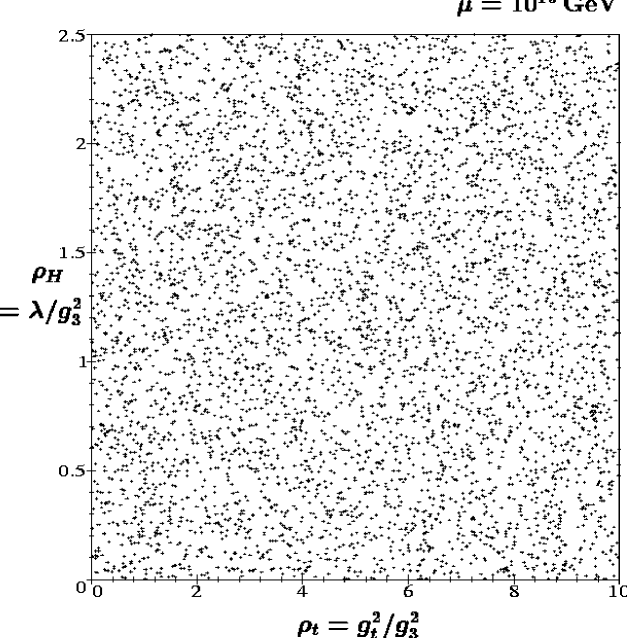
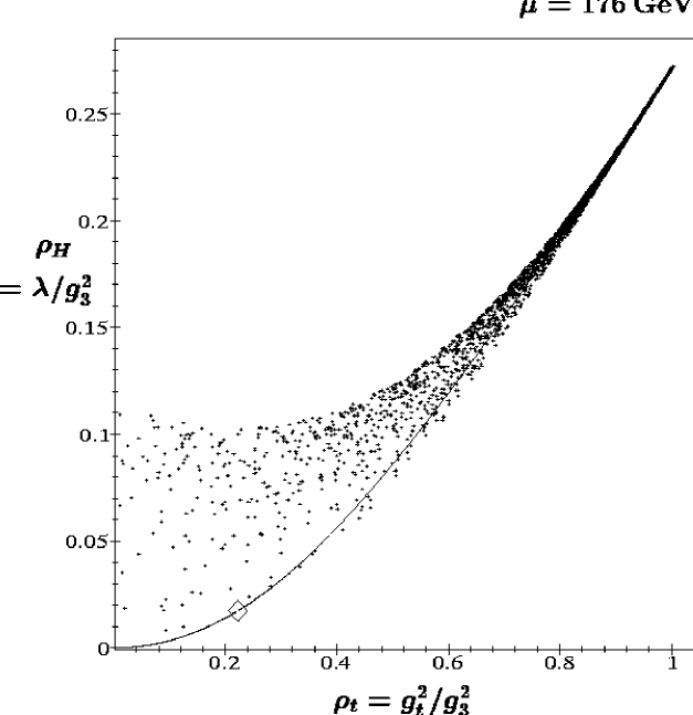
Figure 6: Randomly chosen UV initial values in the $\rho_{H}$-$\rho_{t}$-plane at the UV scale $\mu=\mbox{$\Lambda$}=10^{15}\mbox{$\,{{\rm GeV}}$}$ are subject [109] to the RG evolution down to the IR scale $\mu=176\mbox{$\,{{\rm GeV}}$}$; notice that the UV plane (figure on the left hand side) has scaled down by a factor of 10 to the IR plane (figure on the right hand side). The strong IR attraction of the IR fixed line (fat line with symbol $\Diamond$ for the IR fixed point) is demonstrated. The tip of the line is the absolute upper bound on $\rho_{t}$ and $\rho_{H}$.

A further important question is: if one starts with UV initial values at $\mu=\mbox{$\Lambda$}=10^{15}\mbox{$\,{{\rm GeV}}$}$, say, randomly distributed within the perturbatively accessible large square $0\leq\mbox{$\rho_{t}$}\leq 10$, $0\leq\mbox{$\rho_{H}$}\leq 2.5$, as presented on the left hand side in Fig. 6, how closely do the corresponding IR values at $\mu=\mbox{$m_{t}$}=176\mbox{$\,{{\rm GeV}}$}$ cluster around the IR fixed line? The result is presented on the right hand side in Fig. 6 [109]: notice first that the total range for IR values has shrunk to within a square of one tenth of the length of the UV square, i.e. within a square $0\leq\mbox{$\rho_{t}$}\leq 1$, $0\leq\mbox{$\rho_{H}$}\leq 0.25$. Within this square the points with larger values of $\rho_{t}$ indeed cluster on or very closely to the fixed line (fat line); for lower values of $\rho_{t}$ the points above the line fail to be drawn fully onto the line; their upper boundary is the pendant of the “triviality” bound for $\mbox{$\Lambda$}=10^{15}\mbox{$\,{{\rm GeV}}$}$. (Even though the allusion to a trivial IR fixed point does not apply any more and the notion of an upper bound would be more appropriate we follow the usage in the literature and maintain the expression triviality bound). In comparison with the triviality bound for the Higgs mass, discussed in the framework of the $\phi^{4}$ theory in Subssect. 4.1, the inclusion of the top Yukawa coupling into the discussion has turned the upper Higgs mass bound into a top mass dependent bound [7], [10]. The lower bound, the one-loop vacuum stability bound (see Subsect. 2.6) [7], [11]-[17], is the IR image of all points starting from the UV initial values $R_{0}=0$, i.e. $\lambda_{0}=0$; they all end up very closely to the fixed line (from below!). Thus for this large value $\mbox{$\Lambda$}=10^{15}\mbox{$\,{{\rm GeV}}$}$ for the UV scale the lowest order vacuum stability bound is very close to the IR fixed line; the IR fixed line is clearly an upper bound for the (lowest order) vacuum stability bound. It becomes again clear from Fig. 6 that it is IR attraction of the fixed line rather than of the fixed point (diamond) which determines the “top-down” RG flow.

The outermost tip of the clustering IR points is the IR image of all the UV points with UV initial values $\mbox{$\rho_{t0}$}\geq 1$, i.e. of $90\%$ of the randomly chosen initial values [6], [7], [31], [32], [10], [37], [40], [42]. This is the absolute upper bound as well in $\rho_{t}$ (which had been interpreted as Hill effective fixed point) as well as in $\rho_{H}$, both calculated for $\mbox{$\Lambda$}=10^{15}\mbox{$\,{{\rm GeV}}$}$; this figure clearly demonstrates the attraction power of the upper bound and also that it lies on the IR fixed line [32], [37], [40], [42].

Figure 7: The IR fixed line (fat line) and fixed point (symbol $\Diamond$) in relation to the $\Lambda$ dependent triviality bounds and vacuum stability bounds (thin lines) for UV scale $\mbox{$\Lambda$}=10^{4},\;10^{6},\;10^{10},\;10^{15}\mbox{$\,{{\rm GeV}}$}$, bounding wedge-formed allowed regions. The IR attraction of the bounds towards the IR fixed line is demonstrated. The tip of the wedge, the absolute upper bound on $\rho_{t}$ and $\rho_{H}$ slides down the IR fixed line towards the IR fixed point for increasing values of $\Lambda$.

So far we have discussed a large UV scale, $\mbox{$\Lambda$}=10^{15}\mbox{$\,{{\rm GeV}}$}$. Fig. 7 shows the IR fixed line (fat line) [42] and fixed point (symbol $\Diamond$) [30] in relation to the $\Lambda$ dependent triviality bounds and vacuum stability bounds (thin lines) [6], [7], [10]-[17], [42] for the UV scale $\mbox{$\Lambda$}=10^{4},\;10^{6},\;10^{10},\;10^{15}\mbox{$\,{{\rm GeV}}$}$ within these restricted one-loop considerations. Clearly the $\Lambda$ dependent tip of the wedge slides down the IR line [37], [42] and the triviality and vacuum stability bounds are drawn closer to the IR fixed line for increasing values of $\Lambda$. In the physically inaccessible limit $\mbox{$\Lambda$}\rightarrow\infty$ the upper bound, i.e. the tip of the wedge, is drawn into the Pendleton-Ross fixed point (symbol $\Diamond$).

Obviously, from Figs. 6 and 7, we may conclude that the IR attraction of the fixed line is the dynamical origin for the triviality bound as well as for the vacuum stability bound. They are the boundaries of the points which fail to reach the IR fixed line after evolution with the finite evolution path from the UV scale $\Lambda$ down to the IR scale 176$\,{{\rm GeV}}$.

The discussion for couplings or rather for ratios of couplings may be translated (within the lowest order treated in this section) into results for the top and Higgs masses. The IR fixed line corresponds to an IR attractive RG invariant top-Higgs mass relation. The triviality and vacuum stability bounds, formulated here for the ratios $\mbox{$\rho_{H}$}=\mbox{$\lambda$}/\mbox{$g_{3}^{2}$}$ or $R=\mbox{$\lambda$}/\mbox{$g_{t}^{2}$}$ of couplings, may be translated into corresponding bounds for the Higgs mass as functions of the top mass by means of the lowest order relations $\mbox{$m_{t}$}=\mbox{$g_{t}$}(\mbox{$m_{t}$})v/\sqrt{2}$ and $\mbox{$m_{H}$}=\sqrt{2\mbox{$\lambda$}(\mbox{$m_{H}$})}v$.

The final results for the IR fixed line in the $m_{H}$-$m_{t}$-plane and the corresponding triviality and vacuum stability bounds including all known higher order corrections will be presented in Sect. 6.

Analytical insight into all these features may be obtained [42] from the general solution of the one-loop Riccati differential equation (173) in terms of the IR fixed line solution $\overline{R}$

$$R(\mbox{$\rho_{t}$})=\overline{R}(\mbox{$\rho_{t}$})+\frac{(R_{0}-\overline{R}_{0})\,{\rm exp}[-F(\mbox{$\rho_{t}$},\mbox{$\rho_{t0}$})]}{1+\frac{8}{3}\,(R_{0}-\overline{R}_{0}){\displaystyle\int_{\mbox{$\rho_{t}$}}^{\mbox{$\rho_{t0}$}}}{\rm d}\mbox{$\rho_{t}$}^{\prime}\,{\displaystyle\frac{{\rm exp}[-F(\mbox{$\rho_{t}$}^{\prime},\mbox{$\rho_{t0}$})]}{\mbox{$\rho_{t}$}^{\prime}-\frac{2}{9}}}}$$ (183)

with $R_{0}=R(\mbox{$\rho_{t0}$}),\ \overline{R}_{0}=\overline{R}(\mbox{$\rho_{t0}$})$ and

$$F(\mbox{$\rho_{t}$},\mbox{$\rho_{t0}$})=\frac{1}{3}\int_{\mbox{$\rho_{t}$}}^{\mbox{$\rho_{t0}$}}{\displaystyle\frac{{\rm d}\mbox{$\rho_{t}$}^{\prime}}{\mbox{$\rho_{t}$}^{\prime}-\frac{2}{9}}}(16\overline{R}(\mbox{$\rho_{t}$}^{\prime})+1+{\displaystyle\frac{16}{3}}{\displaystyle\frac{1}{\mbox{$\rho_{t}$}^{\prime}}}).$$ (184)

The difference of any general solution and the fixed line solution, $R(\mbox{$\rho_{t}$})-\overline{R}(\mbox{$\rho_{t}$})$, is given by the second term on the right hand side of Eq. (183), which in turn is controlled by the exponential ${\rm exp}[-F(\mbox{$\rho_{t}$},\mbox{$\rho_{t0}$})]$ in the numerator and the denominator. If the initial value $R_{0}$ happens on the fixed line, i.e. $R_{0}=\overline{R}_{0}$, then clearly $R(\mbox{$\rho_{t}$})=\overline{R}(\mbox{$\rho_{t}$})$, i.e. the solution remains on the fixed line for all values of $\rho_{t}$. For values of $\rho_{t}$ above and below the IR fixed point $\mbox{$\rho_{t}$}=\frac{2}{9}$ $F(\mbox{$\rho_{t}$},\mbox{$\rho_{t0}$})$ is positive and increases with increasing evolution path; this reflects the IR attractiveness of the fixed line. For the discussion of the rate of attraction one has to distinguish two cases:

• $R_{0}-\overline{R}_{0}$ sufficiently small, such that the denominator of Eq. (183) remains close to one; the rate of approach to the fixed line $\overline{R}(\mbox{$\rho_{t}$})$ is given by ${\rm exp}[F(\mbox{$\rho_{t}$},\mbox{$\rho_{t0}$})]$ in the numerator with a behaviour

  • for $\rho_{t}$, $\rho_{t0}$ close to 2/9:

    $${\rm exp}[-F(\mbox{$\rho_{t}$},\mbox{$\rho_{t0}$})]\approx\left(\frac{\mbox{$\rho_{t}$}-\frac{2}{9}}{\mbox{$\rho_{t0}$}-\frac{2}{9}}\;\frac{\mbox{$\rho_{t0}$}}{\mbox{$\rho_{t}$}}\right)^{\sqrt{689}/3} = \left({\displaystyle\frac{\mbox{$g_{3}^{2}$}}{\mbox{$g_{30}^{2}$}}}\right)^{-\frac{1}{7}\sqrt{689}/3}$$ (185)

    $$= \left(1-{\displaystyle\frac{7}{8\pi^{2}}}\mbox{$g_{30}^{2}$}\ln({\displaystyle\frac{\mbox{$\Lambda$}}{\mu}})\right)^{\sqrt{689}/21},$$

    with the high power $\sqrt{689}/3\approx 8.75$ beating the forbiddingly low power 1/7 which monitores the exceedingly slow approach of $\rho_{t}$ towards the IR fixed point 2/9. The resulting fairly large power with respect to $\frac{\mbox{$g_{30}^{2}$}}{\mbox{$g_{3}^{2}$}}$, $\sqrt{689}/21\approx 1.25$, is the appropriate measure for the strength of IR attraction of the fixed line $R(\mbox{$\rho_{t}$})$.

  • for $\mbox{$\rho_{t}$},\ \mbox{$\rho_{t0}$}\geq{\rm O}(1)$:

    $${\rm exp}[-F(\mbox{$\rho_{t}$},\mbox{$\rho_{t0}$})]\approx{\displaystyle(\frac{\mbox{$\rho_{t}$}-\frac{2}{9}}{\mbox{$\rho_{t0}$}-\frac{2}{9}})}^{\sqrt{65}/3}\approx{\displaystyle(\frac{\mbox{$g_{30}^{2}$}}{\mbox{$g_{3}^{2}$}})}^{\frac{1}{7}\sqrt{65}/3}{\displaystyle\frac{1}{\mbox{$\rho_{t0}$}^{\sqrt{65}/3}}}\rightarrow 0\ \ {\rm for}\ \ \mbox{$\rho_{t0}$}\rightarrow\infty$$ (186)

    with a strong rate of IR attraction for sufficiently large $\rho_{t0}$. This is the rate controlling the approach to the upper bound, i.e. the Hill effective fixed point(155) on the fixed line $\overline{R}(\mbox{$\rho_{t}$})$.

• for large $R_{0}-\overline{R}_{0}$, the IR attraction towards the fixed line $\overline{R}(\mbox{$\rho_{t}$})$ is strongly enhanced, due to the substantial increase of the denominator in solution (183). Even for $R_{0}\rightarrow\infty$ the general solution $R(\mbox{$\rho_{t}$})$ is attracted towards the fixed line to within a finite difference

  $$R(\mbox{$\rho_{t}$})\rightarrow\overline{R}(\mbox{$\rho_{t}$})+{\displaystyle\frac{\frac{3}{8}{\rm exp}[-F(\mbox{$\rho_{t}$},\mbox{$\rho_{t0}$})]}{\int_{\mbox{$\rho_{t}$}}^{\mbox{$\rho_{t0}$}}{\displaystyle\frac{{\rm d}\mbox{$\rho_{t}$}^{\prime}}{\mbox{$\rho_{t}$}^{\prime}-\frac{2}{9}}}{\rm exp}[-F(\mbox{$\rho_{t}$}^{\prime},\mbox{$\rho_{t0}$})]}}\ \ {\rm for}\ \ R_{0}\rightarrow\infty,$$ (187)

  which shrinks for increasing length of evolution path (i.e. for increasing value of $\Lambda$). This is the analytical form for the $\Lambda$ dependent triviality bound.

• Likewise, for $R_{0}=0$, the analytical form of the lowest order vacuum stability bound is obtained from Eq. (183)

  $$R(\mbox{$\rho_{t}$})=\overline{R}(\mbox{$\rho_{t}$})+\frac{-\overline{R}_{0}\,{\rm exp}[-F(\mbox{$\rho_{t}$},\mbox{$\rho_{t0}$})]}{1-\frac{8}{3}\,\overline{R}_{0}{\displaystyle\int_{\mbox{$\rho_{t}$}}^{\mbox{$\rho_{t0}$}}}{\rm d}\mbox{$\rho_{t}$}^{\prime}\,{\displaystyle\frac{{\rm exp}[-F(\mbox{$\rho_{t}$}^{\prime},\mbox{$\rho_{t0}$})]}{\mbox{$\rho_{t}$}^{\prime}-\frac{2}{9}}}}\ \ {\rm for}\ \ R_{0}=0.$$ (188)

A final point concerns the hierarchy of IR attraction. The fixed point (174) is in fact the intersection point of two IR attractive lines in the $\rho_{H}$-$\rho_{t}$-plane: the trivial one, $\rho_{t}$=2/9, attracting exceedingly weakly like $(\mbox{$g_{3}^{2}$}/\mbox{$g_{30}^{2}$})^{1/7}$, and the nontrivial one, $\overline{\mbox{$\rho_{H}$}}(\mbox{$\rho_{t}$})$, discussed in this section. This follows a general rule [89]: A fixed point in a plane of two varables is the intersection point of two fixed lines in the plane. The strength of attraction of the two lines is regulated by the coefficients in the coupled differential equations for the two variables. The general case is that one of the fixed lines is more attractive for the RG flow than the other one; the degenerate case in which both are roughly equally attractive, such that the fixed point attracts the RG flow “radially”, is, however, also possible. Coming back to the $\rho_{H}$-$\rho_{t}$-plane: the point to make is that it is gratifying that the physically non-trivial fixed line $\overline{\mbox{$\rho_{H}$}}(\mbox{$\rho_{t}$})$ is more strongly attractive than the more trivial $\rho_{t}$=2/9 fixed line.

4.5 The Top-Bottom-$g_{3}$ Sector of the SM and MSSM
– Top-Bottom Yukawa Coupling Unification as an IR fixed Property

The experimental top mass is much larger than the experimental bottom mass. It is therefore interesting to see, which are the IR attractive fixed manifolds in the top-bottom sector.

Early analyses Refs. [31]-[36] revealed already much of the basic structures, though most of the conclusions were applied to fictitious heavy higher fermion generations. Implicitely the analyses [49]-[65] of the consequences of tau-bottom Yukawa coupling unification in supersymmetric unification for the IR physics single out a narrow band of allowed values in the $\tan\beta$-$m_{t}$-plane which turns out to lie in the vicinity of the IR fixed line in the top-bottom system, to be discussed next. Why this is so and how the results look like will be discussed in Sect. 7. More recent analyses [47],[48] meet the issue by confining the discussion to the IR structure of the RGE in the SM and the MSSM.

Let us begin by a very brief discussion of a setting where the top and bottom Yukawa couplings, $g_{t}$ and $g_{b}$ in the SM and $h_{t}$ and $h_{b}$ in the MSSM, are the only non-zero couplings considered (switching off for the moment also the strong gauge coupling). It is easy to see from the resulting one-loop RG equations that there is a trivial common fixed point, $\mbox{$g_{t}$},\ \mbox{$g_{b}$}=0$, resp. $\mbox{$h_{t}$},\ \mbox{$h_{b}$}=0$, accompanied by an IR fixed line, the solution of the RGE distinguished by the boundary condition that the ratio $g_{t}$/$g_{b}$, resp. $h_{t}$/$h_{b}$ be finite for $\mbox{$g_{t}$},\ \mbox{$g_{b}$}\rightarrow\infty$. It is the line $g_{t}$=$g_{b}$ in the $g_{t}$-$g_{b}$-plane, resp. the line $h_{t}$=$h_{b}$ in the $h_{t}$=$h_{b}$-plane. This fixed line corresponds in this one-loop approximation to exact top-bottom Yukawa coupling unification at all scales $\mu$. This is as it turns out an IR attractive property and a very intriguing result in the light of the recently renewed interest in top-bottom Yukawa unification at the UV scale in the MSSM as motivated from some GUT models.

Such an IR unification is of no interest in the SM, since it would imply in this approximation $m_{t}$=$m_{b}$ which is at strong variance with the experimental situation. The subsequent discussion will show some kind of an “escape route” out of this dilemma.

The top-bottom Yukawa unification is, however, a fascinating and viable option in the MSSM. The additional free parameter $\tan\beta$ allows according to the lowest order Eqs. (45) to have equal Yukawa couplings and any disparity in the masses since in this order

$$\frac{\mbox{$m_{t}$}}{\mbox{$m_{b}$}}=\frac{\mbox{$h_{t}$}}{\mbox{$h_{b}$}}\mbox{$\tan\beta$}$$ (189)

with $\tan\beta$ being largely a free parameter.

After these introductory remarks, let us discuss the much more non-trivial case of three non-zero couplings

$$\mbox{$g_{t}$},\ \mbox{$g_{b}$},\ ,\mbox{$g_{3}$}\neq 0,\ \ {\rm resp.}\ \ \mbox{$h_{t}$},\ \mbox{$h_{b}$},\ \mbox{$g_{3}$}\neq 0,$$ (190)

while all the other couplings are put to zero in the RGE. The discussion follows closely the analysis [47], which was performed in the MSSM.

Again it is economical to consider the following ratios of couplings

$${\rm SM}$$

(191)

which lead to the following partially decoupled form of the RGE

$${\rm SM}$$

.

(192)

The obvious symmetry of the set of equations with respect to the exchange of $g_{t}$ and $g_{b}$, resp. of $h_{t}$ and $h_{b}$, will be reflected in all following results.

Clearly, the system of the two coupled differential equations (192) has a number of fixed points; the only IR attractive one is the following [47];

$${\rm SM}$$

(193)

the other fixed points are

$${\rm SM}$$

(194)

There are two IR fixed lines in the $\rho_{t}$-$\rho_{b}$-plane. The one [47] which will turn out to be the less strongly IR attractive one, does not come as a surprise;

$$\mbox{$\rho_{t}$}=\mbox{$\rho_{b}$}\ \ \ {\rm in\ the\ SM\ and\ the\ MSSM}.$$ (195)

It signifies again top-bottom Yukawa coupling unification for all scales $\mu$ with all the implications already discussed above.

The other one is the solution distinguished by the boundary condition that it be finite$\neq 0$ in the limit $\mbox{$\rho_{b}$}\rightarrow 0$ as well as in the limit $\mbox{$\rho_{t}$}\rightarrow 0$. It is the solution [47] which interpolates the three fixed points

$${\rm SM}$$

   

   

   

(196)

This solution has roughly the shape of a quarter circle. Its end points are the Pendleton-Ross fixed point (154) at $\rho_{b}$=0 and the corresponding mirror symmetric point under the exchange of $\rho_{t}$ with $\rho_{b}$ at $\rho_{t}$=0. The line can be considered as the generalization of the Pendleton-Ross fixed point into the $\rho_{t}$-$\rho_{b}$-plane. In case of the SM this IR fixed line has even an implicit analytical solution

$${\rm For}\ \mbox{$\rho_{b}$}\leq\mbox{$\rho_{t}$}\hskip 28.45274pt\mbox{$\rho_{t}$} = \frac{(\mbox{$\rho_{b}$}-\mbox{$\rho_{t}$})^{2}}{24\mbox{$\rho_{t}$}^{1/2}\mbox{$\rho_{b}$}^{3/2}}\ln\frac{\sqrt{\mbox{$\rho_{t}$}}-\sqrt{\mbox{$\rho_{b}$}}}{\sqrt{\mbox{$\rho_{t}$}}+\sqrt{\mbox{$\rho_{b}$}}}+\frac{1}{12}\frac{\mbox{$\rho_{b}$}+\mbox{$\rho_{t}$}}{\mbox{$\rho_{b}$}},$$ (197)

$${\rm For}\ \mbox{$\rho_{b}$}\geq\mbox{$\rho_{t}$}\hskip 28.45274pt\mbox{$\rho_{t}$} = \frac{(\mbox{$\rho_{b}$}-\mbox{$\rho_{t}$})^{2}}{24\mbox{$\rho_{t}$}^{1/2}\mbox{$\rho_{b}$}^{3/2}}\ln\frac{\sqrt{\mbox{$\rho_{b}$}}-\sqrt{\mbox{$\rho_{t}$}}}{\sqrt{\mbox{$\rho_{b}$}}+\sqrt{\mbox{$\rho_{t}$}}}+\frac{1}{12}\frac{\mbox{$\rho_{b}$}+\mbox{$\rho_{t}$}}{\mbox{$\rho_{b}$}}.$$ (198)

The two IR attractive fixed lines intersect each other in their only common point, the IR attractive fixed point (193).

Next we need some analytical insight into the respective strengths of attraction of the two IR fixed lines as well as of the IR fixed point (193). In absence of an analytical solution one proceeds by linearizing the system (192) of differential equations for $\rho_{t}$ and $\rho_{b}$ in the neighbourhood of the common IR fixed point (193) and by solving it analytically for UV initial values

$$\mbox{$\rho_{t0}$}=\mbox{$\rho_{t}$}(\mu=\mbox{$\Lambda$}),\ \mbox{$\rho_{b0}$}=\mbox{$\rho_{b}$}(\mu=\mbox{$\Lambda$}).$$ (199)

The solutions are [47]

$${\rm SM}$$

(200)

In this approximation the second IR attractive line has the form $\mbox{$\rho_{t}$}+\mbox{$\rho_{b}$}=\frac{1}{3},{\rm resp.}\frac{2}{3}$. One can immediately read off from the approximate analytical solution (200)

• As well in the SM as in the MSSM, the quarter-circle IR attractive line is more attractive, the relevant negative power of $g_{3}^{2}$/$g_{30}^{2}$ being 1/7 to be compared to 1/14 in the SM and 7/9 as compared to 5/9 in the MSSM. Thus the “top-down” RG flow from all UV initial values above and below the fixed line proceeds roughly first towards the quarter-circle fixed line and then close to or along this line towards the IR attractive fixed point (193). Only if the solution happens to start on the $\rho_{t}$=$\rho_{b}$  fixed line it remains on it for the whole evolution path, i.e. for all values $\mu$ between $\Lambda$ and $m_{t}$, leading to top-bottom Yukawa unification at all scales.

• In the SM both exponents, 1/7 as well as 1/14, are exceedingly small, in particular the exponent 1/14 is so ridiculously small (given the evolution from $\Lambda$ to $m_{t}$) that it does not seem to be a serious dilemma that the physical Yukawa couplings are so far from equality. This is the basis of the “escape route” mentioned earlier in this section. This is a practical argument which is, however, not satisfactory from the mathematical point of view.

• The corresponding negative exponents in the MSSM are much larger than in the SM; the quarter circle fixed line attracts with a strength 7/9, the $\rho_{t}$=$\rho_{b}$  fixed line with a strength 5/9.

a)	b)

Figure 8: The more attractive IR fixed line (fat line 1), the less attractive IR fixed line (fat line 2) and the IR attractive fixed point at their intersection (symbol $\Diamond$) in the $\rho_{b}$-$\rho_{t}$-plane of the MSSM. In addition a) The upper bound for $\Lambda$=$M_{{\rm GUT}}$(thin line), playing the role of a Hill type effective fixed line, is shown. b) The “top-down” RG flow, indicated by representative solutions (thin lines), is shown to be first drawn towards the more strongly attractive fixed line line 1 and then close to it or along it towards the IR attractive fixed point. Line 2 implements top-bottom Yukawa unification at all scales $\mu$.

There is again an upper boundary in the $\rho_{t}$-$\rho_{b}$-plane which collects the IR images of solutions with sufficiently large UV initial value $\rho_{t0}$ or $\rho_{b0}$. Since it is essentially independent of sufficiently large UV initial values $\rho_{t0}$ or $\rho_{b0}$ and very strongly attractive, we shall also call it a Hill type effective IR fixed line. The Hill effective fixed point, discussed in Subsect. 4.3, is one point on this line, the point for $\rho_{b0}$=0. Due to the symmetry under exchange of the variables $\rho_{t}$ and $\rho_{b}$, there is a mirror symmetric Hill effective fixed point for $\rho_{t0}$=0. This upper boundary is an IR effective fixed line in the sense that it strongly attracts all solutions of the RGE with sufficiently large initial values $\rho_{t0}$ or $\rho_{b0}$ and that it is independent of those initial values. It is not a genuine IR fixed line since i) it depends on the UV scale $\Lambda$, in fact it shrinks with increasing $\Lambda$ towards the genuine quartercircle shaped fixed line, and ii) it does not attract RGE solutions with smaller initial values $\rho_{t0}$ or $\rho_{b0}$. The Hill type effective fixed line is again dependent on the length of the evolution path, i.e. on $\Lambda$ (in the limit $\mbox{$\Lambda$}\rightarrow\infty$, which is of mathematical interest only, the upper boundary, i.e. the Hill type effective line tends towards the more attractive IR fixed line).

Let us add two illustrative figures for the MSSM. In Figs. 8a) and 8b) we show the two IR fixed lines, the one denoted by 1 is the more attractive one, the one marked by 2 is the less attractive one, which incorporates top-bottom Yukawa unification at all scales $\mu$; their intersection is the IR attractive fixed point, marked by a symbol $\Diamond$. For comparison in Fig. 8a) the upper boundary, playing the role of a Hill type effective fixed line, as calculated for an UV scale $\mbox{$\Lambda$}=\mbox{$M_{{\rm GUT}}$}\approx 2\cdot 10^{16}\mbox{$\,{{\rm GeV}}$}$ is shown. In Fig. 8b) the RG flow, first towards the IR fixed line 1 and then towards the IR fixed point is demonstrated with a selection of general solutions (thin lines). Again the more attractive fixed line appears as the “watershed” between solutions which tend towards infinity for increasing scale $\mu$ and solutions which tend towards zero in the same limit. Fig. 9 in Subsect. 4.6 demonstrates the RG flow in case of the SM. Finally, Fig. 14 in Sect. 6 will show the contraction of UV initial values at $\Lambda$=$M_{{\rm GUT}}$, subject to the MSSM “top-down” two-loop RG evolution, into the close vicinity of the IR fixed lines for the more realistic case where all gauge couplings are included and two-loop RGE equations are used.

An inclusion of the $\tau$ Yukawa coupling into the RGE of the MSSM has been taken into account in Ref. [47]. The fixed point (193) is then supplemented by the trivial fixed point value $\rho_{\tau}$=0, which turns out to be rather strongly attractive, thus justfying a posteriori its omission in the present discussion.

4.6 The Higgs-Top-Bottom-$g_{3}$ Sector of the SM
– a First IR Fixed Surface

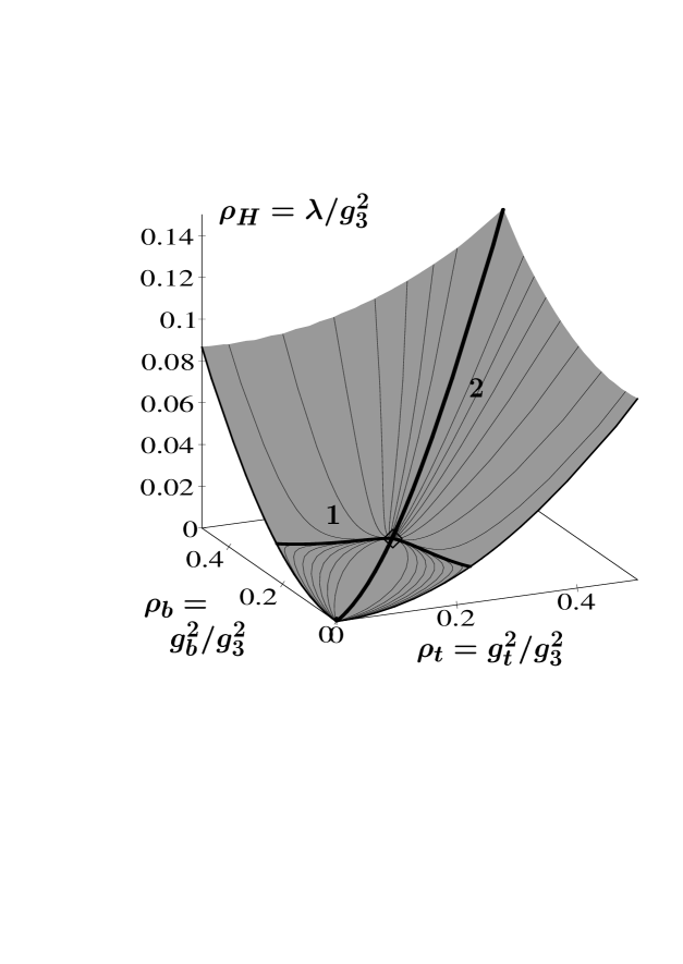
Figure 9: The IR attractive surface in the $\rho_{H}$-$\rho_{b}$-$\rho_{b}$-space containing the more attractive IR fixed line (fat line 1), the less attractive one (fat line 2) and the IR fixed point (symbol $\Diamond$) at their intersection. The “top-down” RG flow is first drawn towards the surface (not shown), then within the surface towards the IR fixed line 1, then along or close to this line towards the IR fixed point, demonstrated by representative solutions (thin lines). The figure was taken from Ref. [48].

Finally, the discussion of

$$\mbox{$\lambda$},\ \mbox{$g_{t}$},\ \mbox{$g_{b}$},\ \mbox{$g_{3}$}\ \neq\ 0$$ (201)

leads us to a reasonable approximation of the SM and to the first IR attractive fixed surface [48]. The one-loop RGE for the three ratio variables $\rho_{H}$=$\lambda$/$g_{3}^{2}$, $\rho_{t}$=$g_{t}^{2}$/$g_{3}^{2}$ and $\rho_{b}$=$g_{b}^{2}$/$g_{3}^{2}$ are given by the Eqs. (192), supplemented by

$${\displaystyle-7\mbox{$g_{3}^{2}$}\frac{{\rm d}\,\mbox{$\rho_{H}$}}{{\rm d}\,\mbox{$g_{3}^{2}$}}}=12\mbox{$\rho_{H}$}^{2}+6\mbox{$\rho_{H}$}\mbox{$\rho_{t}$}+6\mbox{$\rho_{H}$}\mbox{$\rho_{b}$}+7\mbox{$\rho_{H}$}-3\mbox{$\rho_{t}$}^{2}-3\mbox{$\rho_{b}$}^{2}.$$ (202)

The common fixed point [48] of the set of three differential equations is

$$\mbox{$\rho_{t}$}=\mbox{$\rho_{b}$}=\frac{1}{6},\ \ \mbox{$\rho_{H}$}=\frac{\sqrt{89}-9}{24}.$$ (203)

In the space of the three ratio variables $\rho_{H}$, $\rho_{t}$ and $\rho_{b}$ there exists a non-trivial, very strongly IR attractive surface [48], shown in Fig. 9. It is bounded for $\rho_{b}$=0 by the IR attractive fixed line $\overline{\mbox{$\rho_{H}$}}$($\rho_{t}$) in the $\rho_{H}$-$\rho_{t}$-plane as discussed in Subsect. 4.4, and – due to the mirror symmetry of the RGE under the exchange of $\rho_{t}$ and $\rho_{b}$ – for $\rho_{t}$=0 by the corresponding equally IR attractive line $\overline{\mbox{$\rho_{H}$}}$($\rho_{b}$) in the $\rho_{H}$-$\rho_{b}$-plane. For large values of $\rho_{t}$=$\rho_{b}$=$\rho$ it has the expansion

$$\mbox{$\rho_{H}$}(\rho)=\frac{1}{2}\rho-\frac{1}{6}+\frac{1}{36}\frac{1}{\rho}+...\ .$$ (204)

The IR attractive fixed surface fulfils the boundary condition of finite ratios $\rho_{H}$/$\rho_{t}$ and $\rho_{H}$/$\rho_{b}$ for $\rho_{t}$ or $\rho_{b}$ increasing towards infinity. It is the “watershed” between solutions above the surface, for which the ratios $\rho_{H}$/$\rho_{t}$ or $\rho_{H}$/$\rho_{b}$ tend towards infinity, and solutions below the surface which tend towards negative values. Again the IR fixed surface separates the $\rho_{H}$-$\rho_{t}$-$\rho_{b}$-space in two distinct regions: no solution of the RGE can penetrate from above to below the surface or vice versa.

Solutions starting their evolution on the fixed surface, evolve within the surface, independent of the UV initial values $\mbox{$\rho_{H}$}_{0}$, $\rho_{t0}$, $g_{30}^{2}$ and $\Lambda$. The full “top-down” RG flow (not shown in Fig. 9) is first strongly attracted towards the IR fixed surface, from above and from below, and then proceeds on it or close to it as displayed in Fig. 9. Within the surface we rediscover the generalizations of the two IR attractive fixed lines, the more attractive quarter circle line (fat line 1) and the less attractive line $\rho_{t}$=$\rho_{b}$ (fat line 2), which were discussed in Subsect. 4.5. So the RG flow within the fixed surface (indicated by the thin lines for representative solutions in Fig. 9) is towards the more attractive fixed line, from above and from below, and then along or close to it towards the common fixed point (203) denoted by the symbol $\Diamond$.

A last comment concerns again the hierarchy of IR attraction. There are in fact three IR attractive surfaces in the $\rho_{H}$-$\rho_{t}$-$\rho_{b}$-space. The by far most strongly IR attractive non-trivial surface, discussed above, and the two more trivial ones, rising vertically over the quarter circle line and the $\rho_{t}$=$\rho_{b}$ line, respectively, in the $\rho_{t}$-$\rho_{b}$-plane. In fact the fixed lines 1 and 2 in Fig. 9 are each an intersection between the non-trivial and the corresponding more trivial ones. The criterion for which of the three IR attractive surfaces is the most attractive one lies buried in the specific coefficients of the RGE. Again it is gratifying to find the physically most non-trivial surface to be the most strongly IR attractive one.

5 Infrared Fixed Points, Lines, Surfaces in the Presence of All Gauge Couplings

In this section the analyses are extended to include the electroweak gauge couplings $g_{1}$ and $g_{2}$. Before entering the analytical discussion, let us summarize in words the most important development of the last years [43]-[65], [118], [119] concerning the RG flow of the top Yukawa coupling in the MSSM.

• The top down RGE flow of the top Yukawa coupling $\mbox{$h_{t}$}(\mu)$ from large UV initial values $\mbox{$h_{t}$}_{0}\gg 1$ at the UV scale $\Lambda$=$M_{{\rm GUT}}$ is focused essentially into one point at the IR scale $\mu=\mbox{$m_{t}$}=176\mbox{$\,{{\rm GeV}}$}$, $\mbox{$h_{t}$}(176\mbox{$\,{{\rm GeV}}$})\approx 1.1$. This is not all too surprising, since one expects the phenomenon of an upper bound, acting as a Hill effective fixed point [31], as discussed in Subsect. 4.3, also to be present if the electroweak couplings are switched on; it was precisely the power of the Hill effective fixed point to collect the IR images of large UV initial values.

• More surprising is the fact that also smallish UV initial values for the ratio $\mbox{$\rho_{t0}$}=\mbox{$h_{t}$}_{0}^{2}/\mbox{$g_{30}^{2}$}$ are RG evolved upwards towards a larger IR value. A corresponding figure will be supplied later in this section. Thus, e.g. an initial value as small as, say, $\mbox{$h_{t}$}_{0}\approx 0.4$ is evolved towards $\mbox{$h_{t}$}(176\mbox{$\,{{\rm GeV}}$})\approx 0.8$.

• Thus, it is perfectly safe to conclude [43]-[47], [49]-[65], [118], [119] that in the top Yukawa coupling there is a very strongly

  $${\rm IR\ attractive\ fixed\ point\ at}\ \ \ \mbox{$h_{t}$}=O(1)$$ (205)

  which directly leads, with all radiative corrections applied, to the

  $${\rm IR\ attractive\ top\ mass}\ \ \ \mbox{$m_{t}$}=O(190-200)\mbox{$\,{{\rm GeV}}$}\sin\beta.$$ (206)

  The near-at-hand qualitative interpretation, implied to a certain extent also in references quoted above, is that switching on the electroweak gauge couplings effects the genuine Pendleton-Ross type fixed point (154) and the effective Hill fixed point (155) both to move up and to move more closely together, combining their focusing power for the “top-down” RG flow. As we shall see from the following analytical discussion, this is roughly what happens.

• The effect is qualitatively also present in the SM, but the focusing effect for the RG flow is much less pronounced.

The analysis [48] described in the following traces the dynamical origin of these phenomena quasi with a mathematical magnifying glass back to IR attractive fixed manifolds in the spaces of ratios of couplings. In case of the MSSM the analytical insight is much improved, but the practical consequences beyond those known already are somewhat limited. However, in the case of the SM the improved insight allows the exact determination of an IR attractive top mass, Higgs mass and top-Higgs mass relation in presence of the electroweak gauge couplings.

The presentation still sticks to the one-loop RGE, since in that framework all discussed IR fixed manifolds are exact. The appropriate two-loop results as well as their translation into results for the Higgs and fermion masses, mass relations and mass bounds including radiative corrections are reviewed in Sect. 6.

In the following it is again consistently economical to consider the ratios of couplings $\rho_{H}$, $\rho_{t}$, $\rho_{b}$ and $\rho_{\tau}$ introduced in Eqs. (114), supplemented by the ratios

$$\mbox{$\rho_{1}$}=\frac{\mbox{$g_{1}^{2}$}}{\mbox{$g_{3}^{2}$}},\ \ \ {\rm and}\ \ \ \mbox{$\rho_{2}$}=\frac{\mbox{$g_{2}^{2}$}}{\mbox{$g_{3}^{2}$}}.$$ (207)

The one-loop RGE, rewritten for these variables, are

$${\rm SM}$$

,

(208)

where $g_{3}$ is treated as before as a function of $t$, and

$${\rm SM}$$

,

(209)

supplemented within the SM

$${\displaystyle-7\mbox{$g_{3}^{2}$}\frac{{\rm d}\,\mbox{$\rho_{H}$}}{{\rm d}\,\mbox{$g_{3}^{2}$}}} = {\displaystyle 12\mbox{$\rho_{H}$}^{2}+6\mbox{$\rho_{H}$}\mbox{$\rho_{t}$}+6\mbox{$\rho_{H}$}\mbox{$\rho_{b}$}+2\mbox{$\rho_{H}$}\mbox{$\rho_{\tau}$}-\frac{9}{10}\mbox{$\rho_{H}$}\mbox{$\rho_{1}$}-\frac{9}{2}\mbox{$\rho_{H}$}\mbox{$\rho_{2}$}+7\mbox{$\rho_{H}$}}$$ (210)

$${\displaystyle-3\mbox{$\rho_{t}$}^{2}-3\mbox{$\rho_{b}$}^{2}-\mbox{$\rho_{\tau}$}^{2}+\frac{27}{400}\mbox{$\rho_{1}$}^{2}+\frac{9}{40}\mbox{$\rho_{1}$}\mbox{$\rho_{2}$}+\frac{9}{16}\mbox{$\rho_{2}$}^{2}}.$$

In Eqs. (209) and (210) the ratios are treated as functions of the independent variable $g_{3}^{2}$.

The general one-loop solutions for $\rho_{1}$ and $\rho_{2}$ are

$${\rm SM}$$

.

(211)

Let us, for the purpose of mathematical insight, treat for a moment the limit $\mbox{$g_{3}^{2}$}\rightarrow\infty$, which is of course unphysical, since it leads outside the framework of applicability of the perturbative RGE (209) and (210). In this limit, the variables $\rho_{1}$ and $\rho_{2}$ tend towards zero. Thus, the coupled system of differential equations (209), supplemented by Eq. (210) in case of the SM, has a single common IR attractive fixed point (in the unphysical region of the RGE)

$${\rm SM}$$

(212)

which is identical to the one in absence of the electroweak gauge couplings, supplemented by $\rho_{1}$, $\rho_{2}$=0. This feature allows in retrospect the consistent discussion of the RGE in absence of the electroweak gauge couplings (and in absence of the $\tau$ Yukawa coupling) performed in the last section. This circumstance, combined with the knowledge that the electroweak gauge couplings are numerically small in the IR region, might lead one to expect that the systematic inclusion of the electroweak couplings amounts only to a small correction. This is not quite true. Already when including the electroweak couplings by their constant, i.e. non-running, averages [30] or by a more elaborate averaging procedure [42],[47], the position of the IR attractive fixed points is shifted considerably, leading to substantially higher IR attractive top and Higgs mass values. The many analyses [31]-[37],[41],[43]-[65], [118], [119] quoted in the introduction of this section, corroborate this statement in more or less exact frameworks.

There is an intricate reason [48] behind the strong effect of the electroweak gauge couplings: there exist very strongly attractive IR fixed manifolds defined by boundary conditions for large values of $\rho_{1}$ and $\rho_{2}$, which persist to be strongly attractive even in the IR region where $\rho_{1}$ and $\rho_{2}$ are small as compared to one. This is most transparently studied in the case of the top sector in presence of all gauge couplings in the next subsection.

The procedure leading to success starts by treating $\rho_{1}$ and $\rho_{2}$ as free variables in parallel to $\rho_{H}$, $\rho_{t}$, $\rho_{b}$ (and $\rho_{\tau}$). This increases the space of ratio parameters by two dimensions. Such a procedure was put forward for the first time in Refs. [39] in the framework of reduction of parameters to be discussed in Sect. 8. Within this enlarged space the IR attractive fixed subspaces are determined and the full RG flow from the UV to the IR towards these IR manifolds is considered (disregarding for the moment experimentally known initial values for $\rho_{1}$ and $\rho_{2}$). On the one-loop level the resulting IR fixed manifolds are exact. Of course all the IR fixed manifolds terminate in the (unphysical) IR fixed point (212).

The next step will consist in feeding in the experimentally measured initial conditions [5] $\alpha(m_{Z})=1/127.9$ and $sin^{2}\hat{\theta}_{W}(m_{Z})=0.2319\pm 0.0005$ ($\overline{\rm MS}$); ignoring the errors and evolving up to $\mu=\mbox{$m_{t}$}=176\mbox{$\,{{\rm GeV}}$}$, we find

$$\mbox{$g_{1}^{2}$}(\mbox{$m_{t}$}=176\mbox{$\,{{\rm GeV}}$}) = 0.215,\ \mbox{$g_{2}^{2}$}(\mbox{$m_{t}$}=176\mbox{$\,{{\rm GeV}}$})=0.418,\ \ {\rm leading\ to}$$

$$\mbox{$\rho_{1}$}(\mbox{$m_{t}$}=176\mbox{$\,{{\rm GeV}}$}) = 0.160,\ \mbox{$\rho_{2}$}(\mbox{$m_{t}$}=176\mbox{$\,{{\rm GeV}}$})=0.312,$$ (213)

if the initial value (113), $\mbox{$g_{3}^{2}$}(\mbox{$m_{t}$}=176\mbox{$\,{{\rm GeV}}$})=1.34$, is taken into account. This relates $\mbox{$\rho_{1}$}(\mu)$ to $\mbox{$\rho_{2}$}(\mu)$ which will be called henceforth “experimental relation between $\rho_{1}$ and $\rho_{2}$”. Both functions are then known functions of the scale $\mu$, or, more conveniently for our purposes, they become known functions of 1/$g_{3}^{2}$, which in turn is a known function of the scale $\mu$. Finally, for calculating IR attractive top and Higgs mass values, one is interested in evaluating $\rho_{1}$ and $\rho_{2}$ at the IR scale, chosen as $\mu=\mbox{$m_{t}$}=176\mbox{$\,{{\rm GeV}}$}$ in the following, feeding in the values in Eq. (213).

So, finally the $n$-dimensional IR fixed manifold for free variables $\rho_{1}$ and $\rho_{2}$ shrinks to an $n$-2 dimensional manifold if the IR values for $\rho_{1}$ and $\rho_{2}$ are introduced. It is very important to realize that these submanifolds become IR fixed points, lines, surfaces,… in the following sense: the “top-down” RG flow tends more and more closely towards them from above and from below, if the UV scale $\Lambda$ increases, while the IR scale (in our choice) $\mu=\mbox{$m_{t}$}=176\mbox{$\,{{\rm GeV}}$}$) remains constant. In the limit $\mbox{$\Lambda$}\rightarrow\infty$ while keeping the IR scale fixed, which is of mathematical interest only, the full RG flow is drawn onto them.

Let us also point out that the IR scale, chosen as 176$\,{{\rm GeV}}$in the following, is not really a free parameter. In determining the top mass $m_{t}^{{\rm pole}}$ or the Higgs mass $m_{H}^{{\rm pole}}$ from an IR fixed point or fixed line, the appropriate IR scale $\mu$ is determined implicitely from the conditions

$$\frac{v}{\sqrt{2}}\mbox{$g_{t}$}(\mu=\mbox{$m_{t}^{{\rm pole}}$}) = \mbox{$m_{t}^{{\rm pole}}$}(1+\delta_{t}(\mu=\mbox{$m_{t}^{{\rm pole}}$})),$$ (214)

$$v\sqrt{2}\sqrt{\mbox{$\lambda$}(\mu=\mbox{$m_{H}^{{\rm pole}}$})} = \mbox{$m_{H}^{{\rm pole}}$}(1+\delta_{H}(\mu=\mbox{$m_{H}^{{\rm pole}}$}))\ \ {\rm in\ the\ SM},$$ (215)

$$\frac{v}{\sqrt{2}}\mbox{$h_{t}$}(\mu=\mbox{$m_{t}^{{\rm pole}}$})\sin\beta = \mbox{$m_{t}^{{\rm pole}}$}(1+\delta_{t}(\mu=\mbox{$m_{t}^{{\rm pole}}$}))\ \ {\rm in\ the\ MSSM}.$$ (216)

Since, however, the dependence on $\mu$ in $g_{t}$, $\lambda$and $h_{t}$ is only logarithmic, the correction to the result will turn out to be negligible.

Again, for simplicity, $M_{{\rm SUSY}}$=$m_{t}$=176$\,{{\rm GeV}}$ is chosen throughout this section.

5.1 The Top Sector of the SM and MSSM

The minimal and most instructive subsystem of ratios of couplings in the presence of all gauge couplings is $\rho_{t}$, $\rho_{1}$ and $\rho_{2}$. It provides also the basis for the IR fixed point in the top mass of the MSSM, $\mbox{$m_{t}$}=O(190-200)\mbox{$\,{{\rm GeV}}$}\sin\beta$ [44]-[65].

To start with, there are several IR fixed surfaces to be found in the $\rho_{t}$-$\rho_{1}$-$\rho_{2}$ space. The first surface to be put forward in the literature [39] turns out to be not the most strongly IR attractive one. It was found in the framework of parameter reduction, where IR attraction is not a criterion; it will be discussed in Sect. 8.

By far the most strongly IR attractive surface [48] is characterized by its boundary conditions for large values of $\rho_{1}$ and $\rho_{2}$. These limits again lie outside of the region of validity of perturbation theory; however, as we had also experienced in other cases, the surface defined by these boundary conditions determines the properties in the perturbative region.

The origin of this surface is most easily exposed, if first two limiting cases $\rho_{2}$=0, $\mbox{$\rho_{2}$}\neq 0$ and $\rho_{2}$=0, $\mbox{$\rho_{1}$}\neq 0$ are discussed.

For $\rho_{2}$=0, $\mbox{$\rho_{1}$}\neq 0$ a strongly IR attractive line in the $\rho_{t}$-$\rho_{1}$-plane appears with the following properties [48]

$${\rm SM}$$

     

     

(217)

Clearly, this fixed line is strongly IR attractive, since $\rho_{1}$ decreases in its evolution towards the IR; the attraction towards the fixed line is controlled by the large exponent 99/82, resp. 112/99 of $\rho_{1}$. Incidentally the fixed line corresponds to an IR fixed point in the variable

$$\mbox{$\rho_{t}$}/\mbox{$\rho_{1}$}=\mbox{$g_{t}^{2}$}/\mbox{$g_{1}^{2}$},\ {\rm resp.}\ \mbox{$h_{t}^{2}$}/\mbox{$g_{1}^{2}$}.$$ (218)

Similarly instructive is the limit [48], where $\rho_{t}$ is considered as a function of $\rho_{2}$ only with $\rho_{1}$=0, which is even qualitatively different for the SM and the MSSM.

$${\rm SM}$$

     

     

     for large values of  is

     

(219)

Clearly, the fixed point resp. the fixed line is strongly IR attractive: $\rho_{2}$ decreases in its evolution towards the IR and the exponents, 227/266 resp. 4, controlling the attraction, are large.

The resulting two-dimensional IR attractive surface in the $\rho_{t}$-$\rho_{1}$-$\rho_{2}$ plane is bounded by the above mentioned IR fixed lines and fixed point.

The numerical determination of the IR fixed surface in the $\rho_{t}$-$\rho_{1}$-$\rho_{2}$-space is displayed in Fig. 10 for the SM and for the MSSM. The surface merges into the IR fixed point $\rho_{t}$=2/9, $\rho_{1}$=$\rho_{2}$=0 for the SM and into $\rho_{t}$=7/18,$\rho_{1}$=$\rho_{2}$=0 , as all “top-down” RG solutions do. The important point, however, is that the IR fixed surface is much more strongly IR attractive than the IR fixed point. Thus the “top-down” RG flow with free UV initial values for $\rho_{t}$, $\rho_{1}$ and $\rho_{2}$ is first attracted towards the surface and then close to it or along it towards the fixed point.

SM	MSSM

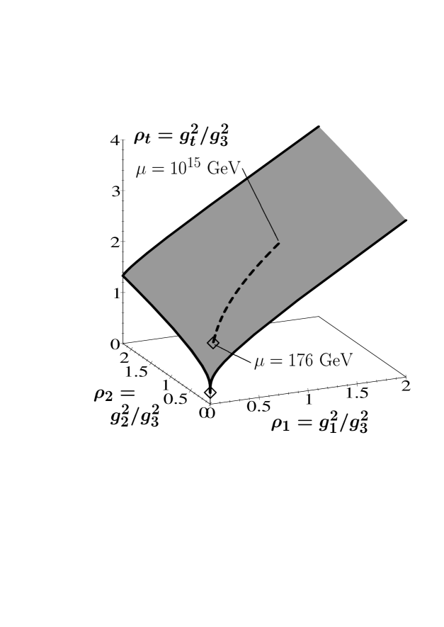
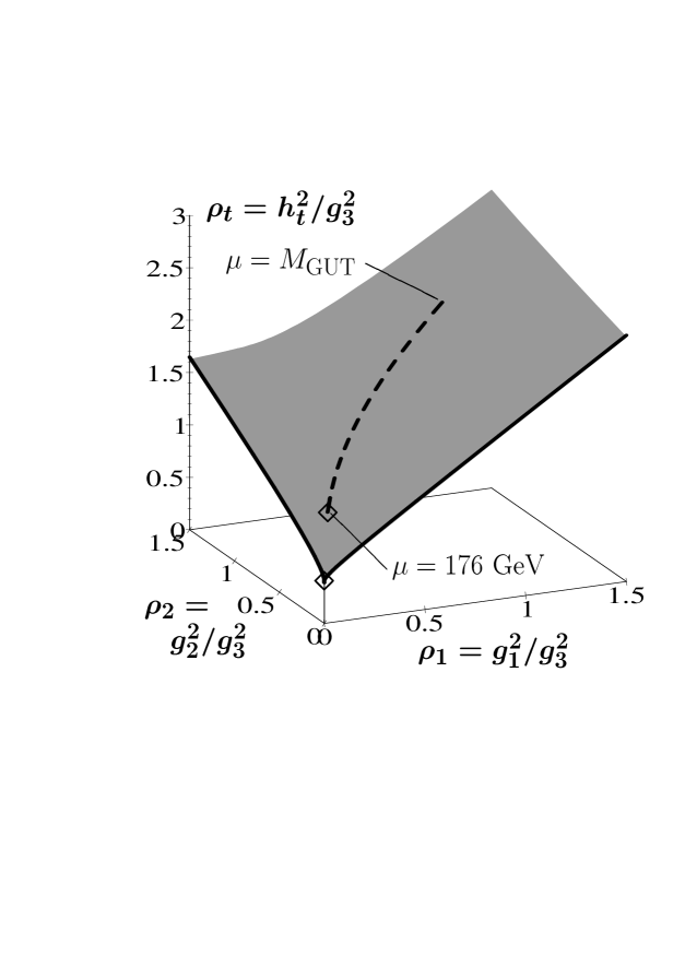
Figure 10: The strongly attractive IR fixed surfaces in the $\rho_{t}$-$\rho_{1}$-$\rho_{2}$-space with $\rho_{1}$ and $\rho_{2}$ considered to be free variables. With the input of the experimental initial values for $\rho_{1}$ and $\rho_{2}$, the evolution of $\rho_{1}$ and $\rho_{2}$ from a high UV scale to the IR scale $\mu=176\mbox{$\,{{\rm GeV}}$}$ traces an IR fixed line (fat broken line) on the surface. At its IR tip is the IR fixed point (symbol $\Diamond$) towards which the RG flow is drawn. The figure was taken from Ref. [48].

SM	MSSM

Figure 11: $\rho_{t}$ as a function of $\mu$ or, more conveniently, as a function of 1/$g_{3}^{2}$. The IR attractive fixed line (fat line) in presence of all gauge couplings, identical with the fat broken in Fig. 10, is shown to attract the RG flow, represented by selected solutions (thin lines). The figure was taken from Ref. [48].

The surface can be represented analytically in various regions by double power series expan- sions . For the SM they are [48]

$${\rm for}\ \mbox{$\rho_{1}$}\rightarrow\infty,\ {\rm around}\ \mbox{$\rho_{2}$}=0\ {\rm in\ powers\ of}\ 1/\mbox{$\rho_{1}$}\ {\rm and}\ \mbox{$\rho_{2}$}$$

$$\rho_{t} = {\displaystyle\frac{11}{10}\mbox{$\rho_{1}$}+\frac{176}{181}-\frac{2150720}{8616143}\frac{1}{\mbox{$\rho_{1}$}}+\frac{99}{362}\mbox{$\rho_{2}$}+\frac{7656563200}{35869003309}\frac{1}{\mbox{$\rho_{1}$}^{2}}+\frac{1298880}{8616143}\frac{1}{\mbox{$\rho_{1}$}}\mbox{$\rho_{2}$}}$$

$$-\frac{384780}{8616143}\frac{1}{\mbox{$\rho_{1}$}}\mbox{$\rho_{2}$}^{2}+...$$

$${\rm for}\ \mbox{$\rho_{1}$}\rightarrow\infty,\ {\rm around}\ \mbox{$\rho_{2}$}=42/19\ {\rm in\ powers\ of}1/\mbox{$\rho_{1}$}\ {\rm and}\ \frac{42}{19}-\mbox{$\rho_{2}$}$$

$$\rho_{t} = \frac{11}{10}\mbox{$\rho_{1}$}+\frac{5423}{3439}-\frac{418655600}{3110427623}\frac{1}{\mbox{$\rho_{1}$}}-\frac{99}{362}(\frac{42}{19}-\mbox{$\rho_{2}$})+\frac{1270201090400}{10696760595497}\frac{1}{\mbox{$\rho_{1}$}^{2}}$$ (221)

$$+\frac{7642800}{163706717}\frac{1}{\mbox{$\rho_{1}$}}(\frac{42}{19}-\mbox{$\rho_{2}$})-\frac{384780}{8616143}\frac{1}{\mbox{$\rho_{1}$}}(\frac{42}{19}-\mbox{$\rho_{2}$})^{2}+...$$

SM	MSSM

Figure 12: The IR attractive fixed line (fat line 1) in presence of all gauge couplings as in Fig. 11 with the IR attractive fixed point (symbol $\Diamond$). In comparison a much less IR attractive line (thin line 2) is shown, which is favoured within the program of reduction of parameters to be discussed in Sect. 8. The figure was taken from Ref. [48].

Feeding in the initial values for $\rho_{1}$, $\rho_{2}$ and $g_{3}^{2}$, the resulting experimental relation between $\rho_{1}$ and $\rho_{2}$ singles out a line in the IR attractive surface in the $\rho_{1}$-$\rho_{2}$-$\rho_{t}$ space, which has been depicted by a fat line in Fig. 10; the line has finite length, running from an UV scale $\Lambda$ down to the IR scale $m_{t}$=176$\,{{\rm GeV}}$. Plotting the $\rho_{t}$ values of the surface along this line as a function of 1/$g_{3}^{2}$ results in the fat line in Fig. 11. Shown are also general solutions representing the RG flow (thin lines).

Here we find first of all the quantitative support for the qualitative discussion led at the beginning of Sect. 5: the “top-down” RG flow from above and from below is focused into a very narrow band of IR values in case of the MSSM. There are many similar figures for the RG flow in the literature [44]-[46], [50]-[65], mostly for the Yukawa coupling $h_{t}$. In case of the SM the focusing effect, though qualitatively similar, is seen to be much less pronounced.

Next let us discuss the effect of the line cut out of the IR attractive fixed surface, (fat broken line in Fig. 10, fat line in Fig. 11) displayed again as the isolated line 1 Fig. 12. It clearly acts like an IR attractive line on this RG flow for all solutions starting from above and from below the line. (This becomes even more evident when persuing the solutions towards large values of $\mu$, where all the solutions above the line are drawn towards it from infinity, while those below the line are drawn towards it from zero). The IR attraction is stronger in the MSSM, as expected from the analytical discussion, and somewhat less strong in the SM.

At the IR scale, $\mu=\mbox{$m_{t}$}=176\mbox{$\,{{\rm GeV}}$}$, the following conclusions can be drawn.

• The IR point (symbol $\Diamond$) on the fixed line 1 in Fig. 12 plays the role of an IR attractive fixed point in presence of the electroweak gauge couplings as well in the SM as in the MSSM. It is a fixed point in the sense that for increasing UV scale $\Lambda$(which is of mathematical interest only), while keeping the IR scale $\mu=\mbox{$m_{t}$}=176\mbox{$\,{{\rm GeV}}$}$ fixed, the RG flow contracts towards this point from below and from above. This fixed point replaces in the presence of the electroweak couplings the Pendleton-Ross fixed point (154).

• The IR image of all solutions starting from a high initial value of $\rho_{t}$ or in other words the effective Hill fixed point in presence of the electroweak gauge couplings, represents the upper bound of all IR points.

• This Hill fixed point is distinctly above the IR fixed point, however, in case of the MSSM very close to it since the IR fixed point is very strongly IR attractive. This was anticipated already in the introduction to Sect. 5. For the SM the distinction has a sizeable effect to be discussed below.

• In the perturbatively inaccessible region below $\mu=\mbox{$m_{t}$}$ the IR fixed line tends towards the genuine IR fixed point at $\rho_{1}$=$\rho_{2}$=0 and $\rho_{t}$=2/9 for the SM resp. $\rho_{t}$= 17/18 for the MSSM, as expected. This part of the line is indicated by small crosses in Fig. 12. The fact that the fixed line rises so strongly between $\rho_{1}$=$\rho_{2}$=0 and the still rather small $\rho_{1}$ and $\rho_{2}$ values (213) at the IR scale is responsible for the strong increase of the IR fixed $\rho_{t}$ value and correspondingly for the IR fixed top mass when switching on the electroweak gauge couplings.

It is worthwhile to translate the positions of the fixed point (symbol $\Diamond$) and of the Hill upper bound in the variable $\rho_{t}$ into top mass values already at this level. One finds from $\mbox{$m_{t}$}(\mu=\mbox{$m_{t}$})=\sqrt{\mbox{$\rho_{t}$}(\mu=\mbox{$m_{t}$})}\mbox{$g_{3}$}(\mu=\mbox{$m_{t}$})(v/\sqrt{2})\sin\beta$ the values of approximately $180\mbox{$\,{{\rm GeV}}$}\sin\beta$ and $190\mbox{$\,{{\rm GeV}}$}\sin\beta$, respectively. These values will be lifted by radiative corrections to $\mbox{$m_{t}^{{\rm pole}}$}\approx 190\mbox{$\,{{\rm GeV}}$}\sin\beta$ and $\mbox{$m_{t}^{{\rm pole}}$}\approx 200\mbox{$\,{{\rm GeV}}$}\sin\beta$, respectively. This shows that the range of values $(190-200)\mbox{$\,{{\rm GeV}}$}\sin\beta$ quoted in the literatur covers the range between the fixed point and the upper bound. It is, however gratifying to see that the IR fixed value lies at the lower end of that range admitting a top mass compatible with the experimental mass within errors even at larger values of $\sin\beta$. (This fact had been pointed out already in an approximate treatment of the inclusion of the electroweak gauge couplings in Ref. [47]).

The enhanced mathematical insight is very advantageous for the SM. There the IR attraction is much weaker than in the supersymmetric case. Therefore the IR fixed point and the Hill effective fixed point are distincly different. It is most appropriate to use the IR fixed point to assign an IR attractive value for top mass in the SM, which will be done in Sect. 6.

5.2 The Top-Bottom Sector of the SM and MSSM

Next the analysis is extended to the top-bottom sector where we expect an IR attractive fixed line at the IR scale. Let us repeat that early results were obtained in Refs. [31]-[36], followed by the analyses[49]-[65] in the framework of supersymmetric grand unification with tau-bottom Yukawa unification to be reviewed in Sect. 7. This framework allowed to trace an allowed region in the $\tan\beta$-$m_{t}$plane which turns out to lie in the vicinity of the IR fixed line. In this section we restrict the discussion again exclusively to the search for the IR manifolds in the RGE of the SM and MSSM; an approximate treatment was given in Ref. [47] for the MSSM, the exact treatment for the SM as well as the MSSM is found in Ref. [48].

The extension of this search to the $\rho_{t}$-$\rho_{b}$ sector leads [48] to a strongly IR attractive three-dimensional subspace in the four dimensional $\rho_{t}$-$\rho_{b}$-$\rho_{1}$-$\rho_{2}$ space (the analogue of Fig. 10 in the $\rho_{t}$-$\rho_{1}$$\rho_{2}$ case). The analytical treatment includes e.g. the boundaries for $\mbox{$\rho_{1}$}\rightarrow\infty$, $\rho_{2}$=0

SM    MSSM

$$\mbox{$\rho_{t}$}=\frac{11}{10}\mbox{$\rho_{1}$}$$ for =0     for =0

for =0 for =0

SM	MSSM

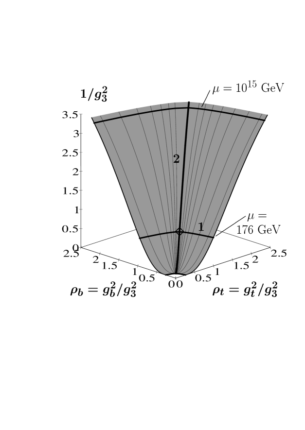
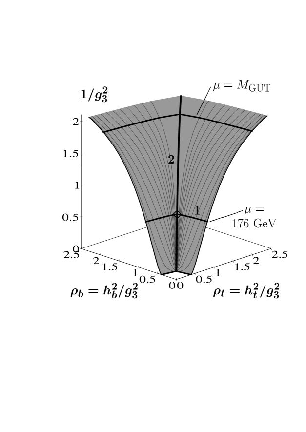
Figure 13: IR attractive fixed surface in the presence of all gauge couplings in the space $\rho_{t}$,$\rho_{b}$ as functions of $\mu$ or 1/$g_{3}^{2}$. Shown are the more attractive IR fixed line (fat line 1), the less attractive fixed line (fat line 2), the latter implementing approximate top-bottom Yukawa unification at all scales $\mu$, the IR fixed point (symbol $\Diamond$) at their intersection. The RG flow within the surface is represented by selected solutions (thin lines). The figure was taken from Ref. [48].

UV	IR

Figure 14: The lattice points are chosen as UV initial values in the $\rho_{t}$-$\rho_{b}$-plane at $\mbox{$\Lambda$}=\mbox{$M_{{\rm GUT}}$}\approx 2\cdot 10^{16}\mbox{$\,{{\rm GeV}}$}$ and subject to the RG evolution of the MSSM in presence of all gauge couplings to the IR scale $\mu=176\mbox{$\,{{\rm GeV}}$}$; notice that the UV plane (figure on the left hand side) has scaled down by a factor of 25 to the IR plane (figure on the right hand side). The very strong IR attraction of the IR fixed line (fat line) and the IR fixed point (symbol $\Diamond$) on it becomes apparent. The upper bound of all lines constitute the Hill effective fixed line. The figure was taken from Ref. [48].

The three-dimensional fixed subspace cannot be represented graphically any more. Injecting the experimental relation between $\rho_{1}$ and $\rho_{2}$ as a function of 1/$g_{3}^{2}$, leads to the projection into a two-dimensional IR attractive fixed surface in the $\rho_{t}$-$\rho_{b}$-1/$g_{3}^{2}$ space, shown in Fig. 13 which attracts the RG flow from above and below. Also displayed are the RG flow within the surface (thin lines), which is followed by solutions which start on the surface or have been attracted onto it. Running down the IR surface to scale $\mu=\mbox{$m_{t}$}$ singles out an IR attractive fixed line in the $\mbox{$\rho_{t}$}(\mu=\mbox{$m_{t}$})$-$\mbox{$\rho_{b}$}(\mu=\mbox{$m_{t}$})$ plane (the fat line 1 in Fig. 13. This line substitutes in the presence of the electroweak gauge couplings the role of the quarter circle fixed line, determined for $\rho_{1}$=$\rho_{2}$=0 in Subsect 4.5. It has a similar shape, but lies at substantially higher values. Again the line and the IR fixed point on it (Diamond) is distingished by the fact that for increasing UV scale $\Lambda$, while keeping the IR scale $\mu=\mbox{$m_{t}$}=176\mbox{$\,{{\rm GeV}}$}$ fixed, the RG flow concentrates more and more closely towards the line and shrinks along the line more and more closely towards the IR fixed point (except for UV initial values $\rho_{t}$=0 or $\rho_{b}$=0). The IR fixed point in $\rho_{t}$  determined for $\rho_{b}$=0 in the last subsection, lies on this IR fixed line at $\rho_{b}$=0. (Evolution into the perturbatively unaccessible region below $\mu=\mbox{$m_{t}$}$, draws all solutions running in the IR attractive surface towards $\rho_{1}$=$\rho_{2}$=0 and the genuine IR fixed lines and finally the genuine IR fixed point in the $\rho_{t}$-$\rho_{b}$ plane discussed in Sect. 4.5).

The resulting IR fixed line (fat line 1 in Fig. 13) is plotted in Fig. 14 as fat line, the IR fixed point is denoted by the symbol $\Diamond$. To be more realistic, the figure contains already the result from a two-loop RGE evolution. Fig. 14 also illustrates the dramatic IR attraction of this fixed line and of the fixed point on it. On the left hand side a dense lattice in the large plane $0\mbox{\,\raisebox{1.29167pt}{$<$}$\!\!\!\!\!$\raisebox{-3.87495pt}{$\sim$}\,}\mbox{$\rho_{t}$},\mbox{$\rho_{b}$}\leq 25$ is shown. The lattice points are taken as UV initial values at the scale $\mbox{$M_{{\rm GUT}}$}\approx 2\cdot 10^{16}\mbox{$\,{{\rm GeV}}$}$. The right hand side shows the IR image of the lattice at the scale $\mu=\mbox{$m_{t}$}=176\mbox{$\,{{\rm GeV}}$}$. Notice first of all that the lattice has shrunk by a factor of 25 in each dimension to within a square $0\mbox{\,\raisebox{1.29167pt}{$<$}$\!\!\!\!\!$\raisebox{-3.87495pt}{$\sim$}\,}\mbox{$\rho_{t}$},\mbox{$\rho_{b}$}\leq 1$. Secondly one sees, how the large initial values $\rho_{t}$ or $\rho_{b}$ have shrunk towards the boundary, the Hill effective fixed line, which is close to the IR fixed line but distinct from it. The IR fixed line is independent of the UV scale $\Lambda$=$M_{{\rm GUT}}$. The Hill effective line, however, reflects the choice $\mbox{$\Lambda$}=\mbox{$M_{{\rm GUT}}$}\approx 2\cdot 10^{16}\mbox{$\,{{\rm GeV}}$}$; in the mathematical limit $\mbox{$\Lambda$}\rightarrow\infty$, while keeping the IR scale fixed, the upper boundary tends towards the IR fixed line. The whole RG flow first is attracted by the IR fixed line from above and below and then proceeds along or close to the IR fixed line towards the IR fixed point (with the exception of the UV initial values $h_{t}$=0 and $h_{b}$=0). The IR fixed line and the upper boundary have moved much closer together in the presence of the electroweak gauge couplings.

Let us also come back to the important issue of the top-bottom Yukawa unification at all scales. The fat line 2 in Fig. 13 signalizes that top-bottom Yukawa unification at all scales $\mu$ survives the inclusion of the electroweak gauge couplings as an approximate property. It is weakly IR attractive. Also the IR fixed point ($\Diamond$) in Figs. 13 and 14 implies approximate top-bottom Yukawa unification at the IR scale $\mu=\mbox{$m_{t}$}=176\mbox{$\,{{\rm GeV}}$}$.

The translation of the results in the $\rho_{t}$-$\rho_{b}$-plane into the $\tan\beta$-$m_{t}^{{\rm pole}}$-plane of the MSSM will be performed in Sect. 6.

5.3 The Higgs-Top-Bottom Sector of the SM

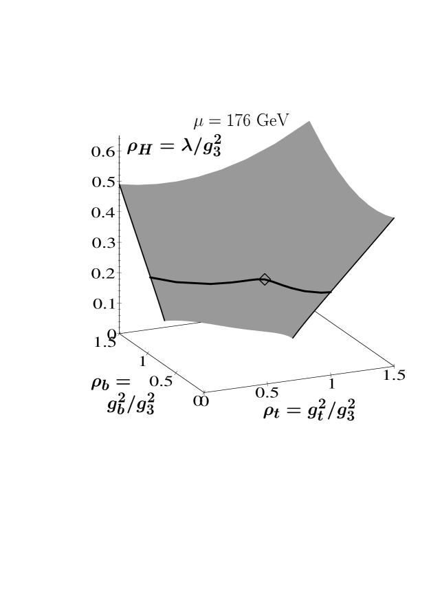
Figure 15: The strongly IR attractive surface in the $\rho_{H}$-$\rho_{t}$-$\rho_{b}$-space at the IR scale $\mu=176\mbox{$\,{{\rm GeV}}$}$ in the presence of all gauge couplings, the IR attractive line (fat line) and the IR attractive fixed point (symbol $\Diamond$). The IR attraction of the RG flow is first towards the fixed surface, then along or close to the surface towards the fixed line and finally along or close to the line towards the fixed point. The figure was taken from Ref. [48].

The two-dimensional IR attractive surface, discussed in the absence of the electroweak gauge couplings, presumably turns into a four-dimensional IR attractive subspace in the five dimensional $\rho_{H}$-$\rho_{t}$-$\rho_{b}$-$\rho_{1}$-$\rho_{2}$ space. Injecting the experimental relation between $\rho_{1}$ and $\rho_{2}$ and evolving down to $\mu=\mbox{$m_{t}$}$ leads to the two-dimensional IR attractive fixed surface in the $\mbox{$\rho_{H}$}(\mu=\mbox{$m_{t}$})$-$\mbox{$\rho_{t}$}(\mu=\mbox{$m_{t}$})$-$\mbox{$\rho_{b}$}(\mu=\mbox{$m_{t}$})$-space shown in Fig. 15, replacing in the presence of the electroweak gauge couplings the surface Fig. 9. The surface in Fig. 15 [48] is again distinguished by the fact that in the (unphysical) limit $\mbox{$\Lambda$}\rightarrow\infty$, while keeping the IR scale fixed, the RG flow is drawn first towards it, then within the surface towards the IR fixed line (fat line) and finally along or close to the line towards the fixed point ($\Diamond$). (Again the IR fixed surface, Fig. 9, is approached in the perturbatively unaccessible region for $\mu$ below $m_{t}$).

6 Infrared Attractive Top and Higgs Masses, Mass Relations and Mass Bounds

The previous sections served to develop the subject step by step pedagogically, still keeping to the one-loop level, since it allows to determine the IR fixed manifolds exactly. Next we are going to review the results on IR attractive top and Higgs mass values and IR attractive mass relations and on Higgs and top mass bounds on the professional level. The present state of the art in most publications is the following.

• Two-loop RGE for the couplings involved are used. At the two-loop level the IR fixed manifolds are mathematically not exact any more, but numerically well-determined within the perturbatively allowed region $\mbox{$m_{t}$}\mbox{\,\raisebox{1.29167pt}{$<$}$\!\!\!\!\!$\raisebox{-3.87495pt}{$\sim$}\,}\mu\mbox{\,\raisebox{1.29167pt}{$<$}$\!\!\!\!\!$\raisebox{-3.87495pt}{$\sim$}\,}\mbox{$\Lambda$}$; they turn out to shifted by at most 10$\%$ with respect to the one-loop ones.

• In order to determine masses from couplings, the two-loop running couplings are first related to the running masses in the $\overline{\rm MS}$ scheme according to the relations (70) for the fermions and (72) for the Higgs boson. Then in most publications the radiative corrections, relating the running masses to the physical pole masses (or at least the most important ones, the radiative QCD corrections to the quark masses), as detailed in Sect. 2.5 are applied. For convenience let us collect the relevant formulae again, including the matching conditions (49) for Yukawa couplings in the MSSM for the transition from the RGE of the SM to the RGE of the MSSM at the scale $M_{{\rm SUSY}}$,

  $$m_{f}(\mu) = \mbox{$m_{f}^{{\rm pole}}$}(1+\delta_{f}(\mu))\;\;\;{\rm with}$$

  $$m_{f}(\mu) = \frac{v}{\sqrt{2}}g_{f}(\mu)=\frac{1}{\sqrt{2\sqrt{2}G_{F}}}g_{f}(\mu);\;\;{\rm for}\;f=t,b,\tau$$

  $$\mbox{$g_{t}$}(\mbox{$M_{{\rm SUSY}}$}^{-}) = \mbox{$h_{t}$}(\mbox{$M_{{\rm SUSY}}$}^{+})\sin\beta,\ \ {\rm in\ case\ of\ the\ MSSM}$$

  $$\mbox{$g_{b}$}(\mbox{$M_{{\rm SUSY}}$}^{-}) = \mbox{$h_{b}$}(\mbox{$M_{{\rm SUSY}}$}^{+})\cos\beta,\ \ {\rm in\ case\ of\ the\ MSSM}$$

  $$\mbox{$g_{\tau}$}(\mbox{$M_{{\rm SUSY}}$}^{-}) = \mbox{$h_{\tau}$}(\mbox{$M_{{\rm SUSY}}$}^{+})\cos\beta\ \ {\rm in\ case\ of\ the\ MSSM}$$

  $$\mbox{$m_{H}$}(\mu) = \mbox{$m_{H}^{{\rm pole}}$}(1+\delta_{H}(\mu))\;\;\;{\rm with}$$

  $$\mbox{$m_{H}$}(\mu) = \sqrt{2\lambda(\mu)}v=\sqrt{\frac{\sqrt{2}}{G_{F}}\mbox{$\lambda$}(\mu)}.$$ (222)

  The choice of the IR scale varies from $\mu=m_{Z}$ to $\mu=\mbox{$m_{t}$}$ in the literature, which can give rise to slight deviations e.g. in the precise determination of mass bounds. Typically the supersymmetry breaking scale $M_{{\rm SUSY}}$ is varied between $m_{t}$ and 1 TeV; for the determination of an upper bound of the light Higgs mass in the MSSM values up to 10 TeV are considered.

• The known bottom and tau masses, Eqs. (6,7), have to be evolved from $\mu=\mbox{$m_{b}$}$, resp. from $\mu=\mbox{$m_{\tau}$}$ up to the IR scale. For this purpose, one makes use of the relations between the running masses and the $\mu$ independent pole masses, collected in Sect. 2.5. (See. e.g. Ref. [55] for a detailed presentation including also a figure of the rather sizeable dependence of $\mbox{$m_{b}$}(\mu=\mbox{$m_{t}$})$ on the initial value for $\alpha_{s}(m_{Z})$, where $\alpha_{s}=\mbox{$g_{3}^{2}$}/(4\pi)$). Notice that the bottom mass quoted in Eq. (6) is the running mass $\mbox{$m_{b}$}(\mu=\mbox{$m_{b}$})$ in the $\overline{\rm MS}$ scheme.

6.1 Top Mass and $\tan\beta$ in the MSSM

Let us start with the more conspicous and well known results in the MSSM, the much-quoted strongly IR attractive fixed point [43]-[65], [118], [119]

$$\mbox{$m_{t}^{{\rm pole}}$}=O(190-200)\mbox{$\,{{\rm GeV}}$}\sin\beta$$ (223)

and a tendency for IR values of $\tan\beta$ to settle around $\mbox{$\tan\beta$}=O(60)$ and the analytical dissection of these results.

In the top-bottom-tau sector at the IR scale to be set for the purpose of the argument at $\mu=\mbox{$m_{t}$}=176\mbox{$\,{{\rm GeV}}$}$, there are four unknown parameters to be considered, the top, bottom and tau Yukawa couplings at $\mu=\mbox{$m_{t}$}=176\mbox{$\,{{\rm GeV}}$}$ and $\tan\beta$. The input of the experimental tau and bottom masses, leads to two unknown parameters at $\mu=\mbox{$m_{t}$}=176\mbox{$\,{{\rm GeV}}$}$, which have been chosen in the literature most sensibly to be $m_{t}^{{\rm pole}}$ and $\tan\beta$. The IR fixed line in the $\rho_{t}$-$\rho_{b}$-plane at $\mu=\mbox{$m_{t}$}$, Fig. 14, can then be translated into an IR fixed line in the $\tan\beta$-$m_{t}^{{\rm pole}}$-plane, Fig. 16 [48], by remembering the definitions $\rho_{t}$=$h_{t}^{2}$/$g_{3}^{2}$ and $\rho_{b}$=$h_{b}^{2}$/$g_{3}^{2}$ and inserting $\mbox{$g_{3}^{2}$}(\mu=\mbox{$m_{t}$})=1.34$ , Eq. (113). Two-loop RGE are used and all radiative corrections are applied (for $h_{\tau}$=0). An approximate treatment had also been given in Ref. [47]. The resulting IR fixed line implies a strongly IR attractive relation between the top mass and the MSSM parameter $\tan\beta$.

Let us emphasize again that the IR fixed line (fat line) is independent of the scale $\Lambda$, while the Hill type effective fixed line (thin line) represents the upper IR bound for $\mbox{$\Lambda$}=\mbox{$M_{{\rm GUT}}$}\approx 2\cdot 10^{16}\mbox{$\,{{\rm GeV}}$}$: in the mathematical limit $\mbox{$\Lambda$}\rightarrow\infty$, while keeping the IR scale fixed, the upper bound along with all other solutions tends towards the fixed line. The IR fixed point, implementing approximate top-bottom Yukawa unification, is denoted by a symbol $\Diamond$ in Fig. 16. The whole RG flow is attracted from above and below very strongly first towards the IR fixed line and then along or close to it towards the IR fixed point (with the exception of the solutions starting from initial values $h_{t}$=0 or $h_{b}$=0).

The results to be read off Fig. 16 are the following [48]

• In the large $\tan\beta$ interval

  $$1\mbox{\,\raisebox{1.29167pt}{$<$}$\!\!\!\!\!$\raisebox{-3.87495pt}{$\sim$}\,}\mbox{$\tan\beta$}\mbox{\,\raisebox{1.29167pt}{$<$}$\!\!\!\!\!$\raisebox{-3.87495pt}{$\sim$}\,}62$$ (224)

  the IR fixed line corresponds to top mass values

  $$150\mbox{$\,{{\rm GeV}}$}\mbox{\,\raisebox{1.29167pt}{$<$}$\!\!\!\!\!$\raisebox{-3.87495pt}{$\sim$}\,}\mbox{$m_{t}^{{\rm pole}}$}\mbox{\,\raisebox{1.29167pt}{$<$}$\!\!\!\!\!$\raisebox{-3.87495pt}{$\sim$}\,}190\mbox{$\,{{\rm GeV}}$}$$ (225)

  well compatible with the experimental top mass (4) within the experimental bounds. A good approximation for the IR fixed line for not too large values of $\tan\beta$ is

  $$\mbox{$m_{t}^{{\rm pole}}$}\approx 192\mbox{$\,{{\rm GeV}}$}\sin\beta.$$ (226)

• The IR fixed point (for $h_{\tau}$=0) lies at

  $$\mbox{$m_{t}^{{\rm pole}}$}\approx 182\mbox{$\,{{\rm GeV}}$},\ \ \ \ \mbox{$\tan\beta$}\approx 60,$$ (227)

  implementing approximate top-bottom unification. This top mass value agrees amazingly well with the experimental value.

• The upper bound, i.e. the Hill type effective fixed line, is very nearby and may be approximately parametrized by

  $$\mbox{$m_{t}^{{\rm pole}}$}\approx 202\mbox{$\,{{\rm GeV}}$}\sin\beta.$$ (228)

Figure 16: The very strongly IR attractive fixed line (fat line) in the $\tan\beta$-$m_{t}^{{\rm pole}}$-plane of the MSSM and the IR attractive fixed point (symbol $\Diamond$) are shown; the fixed point implements approximate top-bottom Yukawa unification. The upper boundary with the interpretation of a Hill type effective fixed line, i.e. the IR image of all large initial values for $h_{t}$ or $h_{b}$ at $\Lambda$=$M_{{\rm GUT}}$, is shown as thin line. The figure was taken from Ref. [48].

Obviously the result (223) quoted in the literature [43]-[65], [118], [119] covers the band of $m_{t}^{{\rm pole}}$ values between the IR fixed line and the upper bound; so, Fig. 16 contains quasi a dissection of this band into a genuine IR fixed line, attracting all solutions, and an upper bound. It is gratifying to notice that the genuine IR fixed line lies at the lower end of $m_{t}^{{\rm pole}}$ values and thus allows a more favourable comparison with the experimental top mass value.

Let us anticipate already that the shape of the band between the IR fixed line and the upper bound in the $m_{t}^{{\rm pole}}$-$\tan\beta$-plane roughly coincides with the band of allowed IR values resulting from the requirement of tau-bottom Yukawa unification [50]-[65] in the framework of supersymmetric grand unification. To this issue we devote Sect. 7, where we review why tau-bottom Yukawa unification focuses the IR physics onto or close to the IR fixed line in the $m_{t}^{{\rm pole}}$-$\tan\beta$-plane.

Here we come back to the knowledge that in determining the top mass $m_{t}^{{\rm pole}}$ from an IR fixed line or point, the IR endpoint of the RG evolution, so far chosen to be 176$\,{{\rm GeV}}$  is in fact not a free parameter: rather the IR scale has to be identical to the top mass $m_{t}^{{\rm pole}}$ which in turn is determined implicitely from the condition (216). Since, however, the dependence on $\mu$ in $h_{t}$ is only logarithmic, the correction to the result is negligible.

This analysis had been performed with $M_{{\rm SUSY}}$=$m_{t}$=176$\,{{\rm GeV}}$and $\alpha_{s}(m_{Z})=0.117$. Of course the result varies if these two parameters are varied. Such a variation will be reviewed in Sect. 7 as well.

Altogether the IR attractive top mass value emerging within the framework of the MSSM is very close to the experimental value and it is gratifying that its IR attraction is so strong. Still, one has to await an experimental confirmation of the supersymmetric scenario and a measurement of $\tan\beta$ before drawing any further conclusions.

6.2 Top and Higgs Masses and Top-Higgs Mass relation in the SM

In the SM the input of the known bottom mass leads to a determination of the Yukawa couplings $g_{b}$ at the IR scale which we shall set, in order to be definite, at $\mu=\mbox{$m_{t}$}=176\mbox{$\,{{\rm GeV}}$}$. With the known input of $\mbox{$g_{3}^{2}$}(\mu=\mbox{$m_{t}$})$, this can be turned into a knowledge of the ratio variable $\rho_{b}$=$g_{b}^{2}$/$g_{3}^{2}$ at $\mu=\mbox{$m_{t}$}$. Now we turn to the two-loop analogue of the IR fixed surface at $\mu=\mbox{$m_{t}$}$ in the Higgs-top-bottom sector, Fig. 9, i.e. in the $\rho_{H}$=$\lambda$/$g_{3}^{2}$-$\rho_{t}$=$g_{t}^{2}$/$g_{3}^{2}$-$\rho_{b}$=$g_{b}^{2}$/$g_{3}^{2}$-space. The insertion of $\rho_{b}$ at $\mu=\mbox{$m_{t}$}$ cuts out of the surface an IR fixed line in the $\rho_{H}$-$\rho_{t}$-plane with a fixed point in it, the fixed line being much more strongly IR attractive than the fixed point. Translating $\rho_{H}$ and $\rho_{t}$ at $\mu=\mbox{$m_{t}$}$ into $\lambda$ and $g_{t}$ at $\mu=\mbox{$m_{t}$}$ and these after inclusion of all radiative corrections into $m_{H}^{{\rm pole}}$and $m_{t}^{{\rm pole}}$, one ends up with the following result in the $m_{H}^{{\rm pole}}$-$m_{t}^{{\rm pole}}$-plane.

• A strongly IR attractive fixed line in the $m_{H}^{{\rm pole}}$-$m_{t}^{{\rm pole}}$-plane, implying a strongly IR attractive top-Higgs mass relation

• and on the fixed line a weakly IR attractive fixed point in the $m_{H}^{{\rm pole}}$-$m_{t}^{{\rm pole}}$-plane, corresponding to IR fixed point top and Higgs mass values. This fixed point plays the role of the Pendleton-Ross fixed point (174) in the presence of the electroweak gauge couplings.

Figure 17: The strongly IR attractive fixed line (fat line) in the $m_{H}^{{\rm pole}}$-$m_{t}^{{\rm pole}}$-plane of the SM and the weakly IR attractive fixed point (symbol $\Diamond$), as well as the triviality and vacuum stability bounds (thin lines) for $\mbox{$\Lambda$}=10^{7},\;10^{11},\;10^{15},\;10^{19}\mbox{$\,{{\rm GeV}}$}$ are shown. The figure was taken from Ref. [48].

The strongly IR attractive top-Higgs mass relation [48] is shown in Fig. 17 (fat line) above $m_{t}^{{\rm pole}}$=150$\,{{\rm GeV}}$. (Below a top mass of 150$\,{{\rm GeV}}$the theoretical determination of the fixed line starts to become unreliable). It may be considered as the non-trivial update of the corresponding figure in Ref. [42]; see also Refs. [32], [40], [37]. The weakly attractive IR fixed point, characterized by a the symbol $\Diamond$ in Fig. 17 is at [48]

$${\rm IR\ attractive\ top\ fixed\ point\ mass}\hskip 28.45274pt\mbox{$m_{t}^{{\rm pole}}$} \approx 214\mbox{$\,{{\rm GeV}}$},$$

$${\rm IR\ attractive\ Higgs\ fixed\ point\ mass}\hskip 28.45274pt\mbox{$m_{H}^{{\rm pole}}$} \approx 210\mbox{$\,{{\rm GeV}}$}.$$ (229)

The IR attractive top mass value is clearly outside the combined one standard deviation errors of the experimental top mass; still it is impressive that the SM, which is not endorsed with an additional free parameter like $\tan\beta$ in the MSSM, has an IR attractive top mass value so relatively close to the experimental value. It has to be stressed, however that this IR fixed point is very weakly attractive, in contradistinction to the top mass fixed point in the MSSM.

The IR fixed line is much more strongly IR attractive than the IR fixed point. So it seems justified to attach more significance to it. Evaluating the line at the experimental top mass value, $m_{t}^{{\rm pole}}$=176$\,{{\rm GeV}}$, say, leads to the corresponding Higgs mass value [48]

$$\mbox{$m_{H}^{{\rm pole}}$}\approx 156\mbox{$\,{{\rm GeV}}$},\ \ {\rm IR\ attractive\ top-Higgs\ mass\ relation,\ evaluated\ at\ \mbox{$m_{t}^{{\rm pole}}$}=176\mbox{$\,{{\rm GeV}}$}}.$$ (230)

This is a very interesting Higgs mass value, but again, experimental confirmation is needed, before any further conclusions can be drawn.

As we had pointed out already in previous sections, the RG flow is first drawn towards the IR fixed line and then close to it or along it towards the IR fixed point. The attraction is stronger above the fixed point than below. This is again reflected in the combined triviality and vacuum stability bounds (thin lines in Fig. 17) for four representative values of $\mbox{$\Lambda$}=10^{7},\ 10^{11},\,10^{15},\ 10^{19}\mbox{$\,{{\rm GeV}}$}$. The allowed region is within the “wedges”. (For the theoretical discussion and the quotation of the relevant literature we refer to Subsects. 2.6, 4.1-4.3). The tip of the wedge is the upper bound, which slides down the IR fixed line for increasing value of the UV scale $\Lambda$ (towards the IR fixed point in the mathematical limit $\mbox{$\Lambda$}\rightarrow\infty$, while keeping the IR scale fixed). (For a thorough discussion of the lower bounds see Subsect. 6.3).

Notice again that the IR scale, set throughout this analysis to $\mu=176\mbox{$\,{{\rm GeV}}$}$, is not a free parameter. Rather the IR scale has to be identical to $m_{t}^{{\rm pole}}$, resp. $m_{H}^{{\rm pole}}$, which in turn is determined implicitely from the condition (214), resp. (215). Since, however, the dependence on $\mu$ in the couplings is only logarithmic, the corrections to the results are very small.

6.3 Lower Bound on the Higgs Mass in the SM

In order to be prepared for future searches for the SM Higgs boson at the LEP200 upgrade of LEP and at the LHC collider, it is important to have a precise analysis of the lower bound, i.e. the vacuum stability bound [7], [11]-[17], on the SM Higgs mass as a function of the top mass and the UV scale $\Lambda$. There are two recent professional analyses in Refs. [15] and [16] (see also Refs. [27] for providing the basis and Ref. [17] for a refinement) which provide such a lower bound and which agree to within a few GeV well within their quoted errors of 3-5$\,{{\rm GeV}}$.

a)	b)
a)	b)

Figure 18: a) Vacuum stability bounds for the SM Higgs mass $m_{H}^{{\rm pole}}$ as a function of the top mass $m_{t}^{{\rm pole}}$ for different values of the UV scale $\Lambda$. b) Limits on the Higgs mass $m_{H}^{{\rm pole}}$ as a function of the UV scale $\Lambda$ for various values of the top mass $m_{t}^{{\rm pole}}$. The figures were taken from Ref. [15].

Figure 19: Vacuum stability bounds for the SM Higgs mass $m_{H}^{{\rm pole}}$ as a function of the top mass $m_{t}^{{\rm pole}}$ for different values of the UV scale $\Lambda$. The figure was taken from Ref. [16].

In both analyses the vacuum stability bound is determined for various UV scales $\Lambda$; both assume the minimal UV scale $\Lambda$  at which new physics could possibly appear without having significant influence at the electroweak scale, to be $\mbox{$\Lambda$}=10^{3}\mbox{$\,{{\rm GeV}}$}$. In this sense the vacuum stability bound for $\mbox{$\Lambda$}=10^{3}\mbox{$\,{{\rm GeV}}$}$ provides the “absolute” lower bound on the Higgs mass. In Ref. [15] the bound was determined from the requirement that the two-loop running Higgs selfcoupling $\mbox{$\lambda$}(\mu)$ reach zero at $\mu=\mbox{$\Lambda$}$, as justified in Sect. 2.6. Ref. [16] used their refined method, leading to a nearly scale independent one-loop effective potential which is RG improved to the next-to-leading order, mentioned at the end of Sect. 2.6. Both include the radiative corrections in relating the running $\overline{\rm MS}$ couplings to the physical Higgs and top pole masses (see the two footnotes in Sect. 2.5 in this context). In Ref. [15] $\alpha_{s}(m_{Z})=0.118$ is used, in Ref. [16] $\alpha_{s}(m_{Z})=0.124$. In Ref. [15] an analytical approximation for the lower Higgs mass bound is given for the two extremal values for $\Lambda$  which allows to vary $m_{t}^{{\rm pole}}$and $\alpha_{s}(m_{Z})$

$$m_{H}^{{\rm pole}} > 135+2.1(\mbox{$m_{t}^{{\rm pole}}$}-174)-4.5\left(\frac{\alpha_{s}(m_{Z})-0.118}{0.006}\right)\ \ {\rm for}\mbox{$\Lambda$}=10^{19}\mbox{$\,{{\rm GeV}}$},$$ (231)

$$m_{H}^{{\rm pole}} > 72+0.9(\mbox{$m_{t}^{{\rm pole}}$}-174)-1.0\left(\frac{\alpha_{s}(m_{Z})-0.118}{0.006}\right)\ \ {\rm for}\mbox{$\Lambda$}=10^{3}\mbox{$\,{{\rm GeV}}$},$$ (232)

in Ref. [16] for comparison

$$\mbox{$m_{H}^{{\rm pole}}$}>127.9+1.92(\mbox{$m_{t}^{{\rm pole}}$}-174)-4.25\left(\frac{\alpha_{s}(m_{Z})-0.124}{0.006}\right)\ \ {\rm for}\ \mbox{$\Lambda$}=10^{19}\mbox{$\,{{\rm GeV}}$}.$$ (233)

The results of the two analyses are exhibited in Figs. 18 and 19, respectively.

One important conclusion is that for a top mass larger than 150$\,{{\rm GeV}}$ the discovery of a SM Higgs boson at LEP200 would imply that the SM breaks down at a scale $\Lambda$ much smaller than a grand unifying scale of $O(10^{15})\mbox{$\,{{\rm GeV}}$}$. Actually, as can be inferred with the additional information about the triviality (upper) bound for the Higgs mass in Fig. 17, for $m_{t}^{{\rm pole}}$=176$\,{{\rm GeV}}$and $\mbox{$\Lambda$}\mbox{\,\raisebox{1.29167pt}{$>$}$\!\!\!\!\!$\raisebox{-3.87495pt}{$\sim$}}\,10^{15}\mbox{$\,{{\rm GeV}}$}$, only a mass range

$$130\mbox{$\,{{\rm GeV}}$}\mbox{\,\raisebox{1.29167pt}{$<$}$\!\!\!\!\!$\raisebox{-3.87495pt}{$\sim$}\,}\mbox{$m_{H}^{{\rm pole}}$}\mbox{\,\raisebox{1.29167pt}{$<$}$\!\!\!\!\!$\raisebox{-3.87495pt}{$\sim$}\,}190\mbox{$\,{{\rm GeV}}$}$$ (234)

is allowed.

6.4 Upper Bound on the Lightest Higgs Mass in the MSSM

The conclusions for the lightest Higgs boson in the MSSM are completely different. This is due to the fact that in the MSSM the tree level mass of the lightest Higgs boson is given in terms of the electroweak gauge couplings, Eq. (51), which reaches maximally the value of the Z boson mass for $\cos^{2}\beta=1$. The remaining task is to calculate the higher order radiative corrections.

a)	b)
c)	d)

Figure 20: The upper bound on the mass $m_{H}^{{\rm pole}}$ of the lightest Higgs mass boson in the MSSM as a function of the top mass $m_{t}^{{\rm pole}}$ for $\cos^{2}\beta=1$ (solid line) and $\cos^{2}2\beta=0$ (dashed line) and values of the supersymmetry scale $M_{{\rm SUSY}}$ and the mixing parameter $X_{t}$: a) $\mbox{$M_{{\rm SUSY}}$}=1\,{\rm TeV}$, $X_{t}=0$, b) $\mbox{$M_{{\rm SUSY}}$}=10\,{\rm TeV}$, $X_{t}=0$, c) $\mbox{$M_{{\rm SUSY}}$}=1\,{\rm TeV}$, $X_{t}^{2}=6\mbox{$M_{{\rm SUSY}}$}^{2}$, d) $\mbox{$M_{{\rm SUSY}}$}=10\,{\rm TeV}$, $X_{t}=6\mbox{$M_{{\rm SUSY}}$}^{2}$. The figure was taken from Ref. [27].

Let us start with a qualitative discussion. The radiative corrections are mainly due to the running of the Higgs selfcoupling according to the (two-loop) RGE of the SM from the scale $\mu=\mbox{$M_{{\rm SUSY}}$}$, where its initial value, Eq. (51), is fixed, to the scale $\mu=\mbox{$m_{H}$}$, in dependence on the size of the top mass. Since the initial value at $\mu=\mbox{$M_{{\rm SUSY}}$}$ is well below the IR attractive Higgs-top mass relation, displayed in Fig. 17, one expects the evolution to increase the Higgs selfcoupling and correspondingly the Higgs mass. The increase will be the stronger, the longer is the evolution path, i.e. the larger is the value for $M_{{\rm SUSY}}$. The upper bound for the Higgs mass, as a function of the top mass, will have to settle below or at best on the IR attractive top-Higgs mass relation.

There is a vast literature on the determination of the higher order radiative corrections [18]-[28] which cannot all be reviewed here. We shall concentrate on the results of a recent, very careful analysis [27]. In Ref. [27] the supersymmetry breaking scale is assumed to be well above the lightest Higgs mass; $\mbox{$M_{{\rm SUSY}}$}=1\,{\rm TEV}$ and $\mbox{$M_{{\rm SUSY}}$}=10\,{\rm TEV}$ are the values for which results are presented. The authors [27] include the one-loop threshold contribution due to a possible stop mixing at $M_{{\rm SUSY}}$in the following form,

$$\Delta\mbox{$\lambda$}=\frac{3\mbox{$h_{t}$}^{4}}{16\pi^{2}}\frac{X_{t}^{2}}{\mbox{$M_{{\rm SUSY}}$}^{2}}\left(1-\frac{X_{t}^{2}}{12\mbox{$M_{{\rm SUSY}}$}^{2}}\right),$$ (235)

This term has to be added to the initial value for the tree level Higgs selfcoupling at $\mu=\mbox{$M_{{\rm SUSY}}$}$ on the right hand side of Eq. (51). $X_{t}$ is a measure of the stop mixing. The authors consider two extreme values for $X_{t}$, $X_{t}^{2}=6\mbox{$M_{{\rm SUSY}}$}^{2}$ for maximal threshold effects and $X_{t}=0$, for absence of mixing.

They use the framework [27] of an almost scale independent one-loop effective potential, RG improved at the two-loop level, which has been quoted already in Sects. 2.6 and 6.3, and include the full radiative corrections relating the $\overline{\rm MS}$ masses to the physical pole masses $m_{H}^{{\rm pole}}$ and $m_{t}^{{\rm pole}}$. Since the tree level Higgs mass lies well below the IR attractive fixed line in the $m_{H}^{{\rm pole}}$-$m_{t}^{{\rm pole}}$-plane, Fig. 17, the RG evolution from $\mu=\mbox{$M_{{\rm SUSY}}$}$ down to $\mu=\mbox{$m_{H}$}$ gives positive corrections. Fig. 20 shows the result of the analysis. The bound depends on the parameters $M_{{\rm SUSY}}$, $X_{t}$ and $\cos^{2}2\beta$ and of course on $m_{t}^{{\rm pole}}$.

An analytic approximation for the most conservative bound is [27]

$$\mbox{$m_{H}^{{\rm pole}}$}<126.1+0.75(\mbox{$m_{t}^{{\rm pole}}$}-174)-0.85\left(\frac{\alpha_{s}(m_{Z})-0.124}{0.006}\right)$$ (236)

which can be compared with the lower bounds on the SM Higgs mass discussed in Sect. 6.3. For a top mass of order of 176$\,{{\rm GeV}}$ the upper bound on the Higgs mass is of the order of 130$\,{{\rm GeV}}$.

7 Supersymmetric Grand Unification Including Yukawa Unification

As has been developed in Sect. 2.3, an interesting tool to constrain the “top-bottom” RG flow by symmetry relations between initial values at the UV scale is provided in the framework of minimal supersymmetric grand unification implying in addition tau-bottom or even tau-bottom-top Yukawa unification. Recent analyses have been performed in the gauge sector [78],[55],[73],[58],[74] and including Yukawa coupling unification, more recently combined with the issue of an IR attractive top mass, [49]-[65]. Most of them go beyond the framework considered in this review and cover in addition issues like i) inclusion of all fermion masses and mixing angles into the analysis and investigation of the quantitative implications of ansätze (textures) for the fermion mass matrix at the grand unification scale $M_{{\rm GUT}}$ with tau-bottom Yukawa unification implemented, ii) exploration of the Higgs sector, iii) implementation of a realistic supersymmetric particle spectrum, iv) radiative electroweak symmetry breaking, v) search for IR fixed points in the supersymmetry breaking mass terms or vi) investigation of the fixed point structure of the underlying gauge theory. We are going to lead the discussion for the heaviest fermion generation only within the framework outlined in Sect. 2.

These analyses have two global aspects.

• They represent a crucial test of supersymmetric grand unification including tau-bottom (-top) Yukawa unification at the quantitative level.

• More interestingly in the context of this review, they demonstrate that tau-bottom unification requires the IR values for the top mass to be close to its IR fixed point or, more generally, the IR values in the $\tan\beta$-$m_{t}^{{\rm pole}}$-plane to be close to the IR fixed line discussed in Subsect. 6.1.

The program involves several steps. A first step is the exploration [78], [55],[73],[58],[74] of gauge coupling constant unification (52). The preferred way to perform this analysis is to assume gauge coupling constant unification (52) at a scale $M_{{\rm GUT}}$ which at this stage is not specified; so there are two unknown parameters, the unified gauge coupling at $\mu=\mbox{$M_{{\rm GUT}}$}$ and the unification scale $M_{{\rm GUT}}$ itself; in addititon there is a mild dependence on the supersymmetry breaking scale $M_{{\rm SUSY}}$ which regulates the transition from the RGEs of the MSSM to those of the SM. These parameters are adjusted such that the two-loop RG evolution of the MSSM gauge couplings, including among others the two-loop contribution of the large top Yukawa coupling, leads to the experimental values for $\alpha(m_{Z})$ and $\sin^{2}\theta_{W}$; this procedure results in a value for $M_{{\rm GUT}}$ and for $\alpha_{s}(m_{Z})$, both depending mildly on $M_{{\rm SUSY}}$. As has been stressed in Ref. [73],[58],[74] it is important to estimate the theoretical error for $\alpha_{s}(m_{Z})$, allowing for a variation of $M_{{\rm SUSY}}$ within reasonable bounds and for threshold corrections and nonrenormalizable operator corrections at the low and high scales. A most recent analysis [74] along these lines determines $M_{{\rm GUT}}$ to be $\mbox{$M_{{\rm GUT}}$}\simeq 3\cdot 10^{16}\mbox{$\,{{\rm GeV}}$}$ and $\alpha_{s}(m_{Z})$ with the appropriate theoretical errors to be

$$\alpha_{s}(m_{Z})\simeq 0.129\pm 0.010,$$ (237)

which is larger than the experimental value, however, still within the experimental and theoretical errors.

The analysis so far fixes the gauge sector and $M_{{\rm GUT}}$, having used the experimental value of the top quark mass already for the two-loop contribution of the top Yukawa couplings to the RGE of the gauge couplings.

Next, the two-loop RGEs for the heavy fermion generation, the tau, bottom and top quark are considered. There are to start with four completely free parameters, the initial values for the top, bottom and tau Yukawa couplings at the unification scale $M_{{\rm GUT}}$, say, and the parameter $\tan\beta$, characterizing the ratio of the two different Higgs vacuum expectation values in the supersymmetric theory; a further rather constrained parameter is the value of $M_{{\rm SUSY}}$.

Now, the tau-bottom Yukawa unification (53)

$$\mbox{$h_{\tau}$}(\mu=\mbox{$M_{{\rm GUT}}$})=\mbox{$h_{b}$}(\mu=\mbox{$M_{{\rm GUT}}$}),$$ (238)

is introduced as well as the known tau and bottom masses within their errors, Eqs. (6,7).

What happens then is rather subtle (see e.g. Ref. [55] for a comprehensive presentation) and requires some preparatory remarks. In Subsect. 2.5 and the introduction to Sect. 6 we have seen, how to translate the given input of the top and bottom masses into the MSSM bottom and $\tau$ Yukawa couplings at some higher scale $\mu$. For definiteness, let us fix $M_{{\rm SUSY}}$=$m_{t}$=176$\,{{\rm GeV}}$. Then the MSSM bottom and $\tau$ Yukawa couplings at this scale are given as follows

$$\mbox{$m_{b}$}(\mu=\mbox{$m_{t}$}) = \frac{v}{\sqrt{2}}\,\mbox{$h_{b}$}(\mu=\mbox{$m_{t}$})\cos\beta,$$ (239)

$$\mbox{$m_{\tau}$}(\mu=\mbox{$m_{t}$}) = \frac{v}{\sqrt{2}}\,\mbox{$h_{\tau}$}(\mu=\mbox{$m_{t}$})\cos\beta.$$ (240)

in terms of the unknown parameter $\cos\beta$. Now, one realizes that the input of tau-bottom Yukawa unification on the one hand and of the tau and bottom masses on the other hand leads to fixing the ratio

$$R_{b/\tau}(\mu)=\frac{\mbox{$h_{b}$}(\mu)}{\mbox{$h_{\tau}$}(\mu)}$$ (241)

at two scales

$$R_{b/\tau}(\mu=\mbox{$M_{{\rm GUT}}$}) = 1\hskip 85.35826pt{\rm and}$$

$$R_{b/\tau}(\mu=\mbox{$m_{t}$}) = \frac{\mbox{$m_{b}$}(\mu=\mbox{$m_{t}$})}{\mbox{$m_{\tau}$}(\mu=\mbox{$m_{t}$})}.$$ (242)

The input of two initial values for the same quantity $R_{b/\tau}(\mu)$ at two different scales $\mu$ can only be accommodated, by tuning the contribution of the top Yukawa coupling $\mbox{$h_{t}$}(\mu)$, which enters the RGE of $h_{b}$ on the one-loop level and is absent from the one-loop RGE of $h_{\tau}$. This can be made most transparent analytically [56],[55] by looking at the one-loop RGE for $R_{b/\tau}$

$$\frac{{\rm d}\,R_{b/\tau}}{{\rm d}\,t}=\frac{R_{b/\tau}}{16\pi^{2}}\left(\frac{4}{3}\mbox{$g_{1}^{2}$}-\frac{16}{3}\mbox{$g_{3}^{2}$}+\mbox{$h_{t}^{2}$}+3\mbox{$h_{b}^{2}$}-3\mbox{$h_{\tau}^{2}$}\right),$$ (243)

the solution of which has to accommodate the two initial values (242). For small $\tan\beta$ the bottom and tau Yukawa couplings do not play a significant role in this RGE. As the running gauge couplings are fixed at $\mu=\mbox{$m_{t}$}$ and $\mu=\mbox{$M_{{\rm GUT}}$}$ and thus not available for the fine tuning of the initial values (242), clearly the contribution [52],[53],[54],[55]

$$\exp\left(\frac{1}{16\pi^{2}}\int\limits_{\mbox{$m_{t}$}}^{\mbox{$M_{{\rm GUT}}$}}{\rm d}\ln\mu\;\mbox{$h_{t}^{2}$}(\mu)\right)$$ (244)

is crucial in the fine tuning of the ratios $R_{b/\tau}(\mbox{$M_{{\rm GUT}}$})$ and $R_{b/\tau}(\mbox{$m_{t}$})$ to their values prescribed by tau-bottom unification and the bottom and tau masses, respectively. Now, the running of the top Yukawa coupling $\mbox{$h_{t}$}(\mu)$ is in principle not free to choose, it has to satisfy its own RGE in the system of coupled first order differential equations and furthermore the product $(v/\sqrt{2})\mbox{$h_{t}$}(\mu=\mbox{$m_{t}$})\sin\beta$ involving its initial value $\mbox{$h_{t}$}(\mu=\mbox{$m_{t}$})$, adorned with the appropriate radiative corrections, is required to match the experimental top mass.

Now comes the key observation which provides a way out: the RGE for $\mbox{$h_{t}$}(\mu)$ exhibits the strongly attractive IR fixed point, discussed at length in Sects. 3-6 and this fixed point is, as we know, well compatible with the experimental value for $m_{t}$. Setting the IR value $\mbox{$h_{t}$}(\mu=\mbox{$m_{t}$})$ onto or close to the fixed point value, admits practically any sufficiently large UV starting value $\mbox{$h_{t}$}(\mbox{$M_{{\rm GUT}}$})$. This circumstance allows to adjust the UV value $\mbox{$h_{t}$}(\mu=\mbox{$M_{{\rm GUT}}$})$ such as to accommodate the ratios $R_{b/\tau}(\mbox{$M_{{\rm GUT}}$})$ and $R_{b/\tau}(\mbox{$m_{t}$})$ as prescribed by tau-bottom unification and the bottom and tau masses, respectively, without altering the IR value $\mbox{$h_{t}$}(\mu=\mbox{$m_{t}$})$ and without fixing the free parameter $\tan\beta$.

As it turns out, the accommodation of the two conditions (242) implies rather large values for the UV initial value $h_{t}$($M_{{\rm GUT}}$). There is a tight corner in the analysis: the necessary value for $h_{t}$($M_{{\rm GUT}}$) depends sensitively on the value of $\mbox{$m_{b}$}(\mbox{$m_{t}$})$ which in turn depends on $\alpha_{s}(m_{Z})$ (via the evolution of $m_{b}$ from $\mu=\mbox{$m_{b}$}$ to $\mu=\mbox{$m_{t}$}$): the required value for $\mbox{$h_{t}$}(\mbox{$M_{{\rm GUT}}$})$ increases with $\alpha_{s}(m_{Z})$ and for $\alpha_{s}(m_{Z})$ increasing beyond the value 0.12 the top Yukawa coupling $\mbox{$h_{t}$}(\mbox{$M_{{\rm GUT}}$})$ becomes so large that it leaves the safe region of perturbation theory. This casts doubt on the perturbative unification.

For larger values of $\tan\beta$ the bottom Yukawa coupling becomes relevant besides the top Yukawa coupling on the right hand side of the differential equation (243). Fortunately, there is a whole IR fixed line available in the $\rho_{t}$-$\rho_{b}$ plane, viz. in the $h_{t}$-$h_{b}$ plane, which may take over for larger values of $\tan\beta$ the role of the IR fixed point in the argument led for small values of $\tan\beta$ above. This is exactly what happens. From the discussion in Sects. 5.2 and 6.1 one would expect that for any value $\mbox{$\tan\beta$}\mbox{\,\raisebox{1.29167pt}{$<$}$\!\!\!\!\!$\raisebox{-3.87495pt}{$\sim$}\,}50-60$ there should be an IR starting point on or close to the half-circle type IR fixed line in the $h_{t}$-$h_{b}$ plane, resp. in its translation into the $\tan\beta$-$m_{t}^{{\rm pole}}$-plane, which similarly allows to accommodate the two initial values (242) for the ratio $R_{b/\tau}$. As announced in Sects. 4.5, 5.2 and 6.1, the exploitation [49]-[65] of the consequences of tau-bottom Yukawa unification for the IR physics isolates narrow allowed bands of IR values in the $\tan\beta$-$m_{t}^{{\rm pole}}$-plane, which turn out to be close to the IR attractive fixed line as translated into the $\tan\beta$-$m_{t}^{{\rm pole}}$-plane. So in this very implicit way the IR attractive fixed line in the $\tan\beta$-$m_{t}^{{\rm pole}}$-plane had been isolated without explicitely having been recognized as such.

Let us present typical results from Refs. [55],[63],[58]. They are represented in form of allowed regions in the $\tan\beta$-$m_{t}^{{\rm pole}}$-plane at a suitable IR scale. The analyses are based on the two-loop RGE of the MSSM, the grand unification scale is determined by the unification of the electroweak gauge couplings and $\alpha(m_{Z})$ is treated as a free parameter. In Refs. [55], [63] the IR scale was chosen to be $m_{t}$=150$\,{{\rm GeV}}$and the analysis was performed for two values of the supersymmetry breaking scale, $M_{{\rm SUSY}}$=$m_{t}$=150$\,{{\rm GeV}}$and $\mbox{$M_{{\rm SUSY}}$}=1\,{\rm TeV}$, and two values of $\alpha(m_{Z})$, $\alpha(m_{Z})=0.11$ and $\alpha(m_{Z})=0.12$. The input bottom mass was chosen according to Eq. (6) as $4.25\pm 0.15\mbox{$\,{{\rm GeV}}$}$. For this narrow band of bottom mass values the requirement of tau-bottom unification admits a narrow allowed bands in the $\tan\beta$-$m_{t}$-plane shown as a narrow dark region in Fig. 21 for a) $M_{{\rm SUSY}}$=$m_{t}$, $\alpha_{s}(m_{Z})=0.11$, b) $M_{{\rm SUSY}}$=$m_{t}$, $\alpha_{s}(m_{Z})=0.12$, c) $\mbox{$M_{{\rm SUSY}}$}=1\,{\rm TeV}$, $\alpha_{s}(m_{Z})=0.11$, d) $\mbox{$M_{{\rm SUSY}}$}=1\,{\rm TeV}$, $\alpha_{s}(m_{Z})=0.12$. Obviously, the allowed region is shifted towards larger top masses for increasing scale $M_{{\rm SUSY}}$and for inreasing $\alpha(m_{Z})$. The top mass in these figures is not $m_{t}^{{\rm pole}}$but rather $\mbox{$m_{t}$}(\mu=\mbox{$m_{t}$})$, so about $5\%$ have to be added in order translate to it into $m_{t}^{{\rm pole}}$. The corresponding updated figure [63] in the $\tan\beta$-$m_{t}^{{\rm pole}}$-plane for $M_{{\rm SUSY}}$=$m_{t}$=150$\,{{\rm GeV}}$and $\alpha(m_{Z})=0.12$ is shown in Fig. 22. In Ref. [58] the ansatz

$$\mbox{$m_{b}$}(5\mbox{$\,{{\rm GeV}}$})=\rho^{-1}\mbox{$m_{b}$}^{0}(5\mbox{$\,{{\rm GeV}}$})\leq 4.45\mbox{$\,{{\rm GeV}}$},$$ (245)

was made, where $\mbox{$m_{b}$}^{0}$ is the prediction for $m_{b}$ without the theoretical corrections incorporated in the parameter $\rho^{-1}$. This correction parameter is to incorporate all uncertainties in the running from $m_{Z}$ up to $M_{{\rm GUT}}$; a theoretical estimate leads to $\rho^{-1}=0.85$ as reasonable value. The resulting allowed region for $\alpha(m_{Z})=0.12$ is shown in Fig. 23.

A comparison e.g. of Fig. 22 with Fig. 16 shows that indeed tau-bottom Yukawa unification requires the IR result of the “top-down” RG flow to lie on or close to the IR fixed line. A closer look reveals that it is rather the upper bound, the Hill effective fixed line, which is determined from the analyses implementing tau-bottom unification.

A final issue is the tau-bottom-top Yukawa unification (54) within supersymmetric grand unification. In this context it is a symmetry constraint $\mbox{$h_{t}$}(\mu=\mbox{$M_{{\rm GUT}}$})=\mbox{$h_{b}$}(\mu=\mbox{$M_{{\rm GUT}}$})$ for the UV initial values of $h_{t}$ and $h_{b}$, required to hold in addition to the tau-bottom Yukawa unification. In Sects. 4.5 and 5.2 an IR attractive fixed line was isolated which implements approximate top-bottom Yukawa unification at all scales $\mu$; correspondingly we expect the top-bottom Yukawa unification input at $\mu=\mbox{$M_{{\rm GUT}}$}$ to persist down to the IR scale. Indeed, the analysis [63], Fig. 22, shows that the IR image of combined tau-bottom-top Yukawa unification at the UV scale is at large values of $\tan\beta$, i.e. in the vicinity of the IR fixed point in Fig. 16.

Altogether the following features emerge from the analyses described and figures shown

• Grand unification of gauge couplings requires the strong gauge coupling $\alpha_{s}(m_{Z})$ to be rather large, but still within the experimental and theoretical errors. Taking the central value $\alpha_{s}(m_{Z})=0.129$ emerging from the most recent analysis of this kind at face value, tau-bottom Yukawa unification requires UV top Yukawa couplings which are too large to lead to perturbatively reliable results.

• In a setting, where only unification of the electroweak gauge couplings is required and $\alpha_{s}(m_{Z})$ is allowed to vary between the values 0.11 and 0.12, tau-bottom Yukawa unification may be implemented. As a consequence the allowed IR parameters become tightly constrained as a function of the bottom mass value and a weak function of the supersymmetry breaking scale $M_{{\rm SUSY}}$ and the value of $\alpha_{s}(m_{Z})$. Taking Fig. 22 as a guideline and the experimental top mass (4), $m_{t}$=176$\,{{\rm GeV}}$with errors, at face value, two narrow windows for solutions for $\tan\beta$ remain, one at small values $1\mbox{\,\raisebox{1.29167pt}{$<$}$\!\!\!\!\!$\raisebox{-3.87495pt}{$\sim$}\,}\mbox{$\tan\beta$}\mbox{\,\raisebox{1.29167pt}{$<$}$\!\!\!\!\!$\raisebox{-3.87495pt}{$\sim$}\,}4$ and one at large values $42\mbox{\,\raisebox{1.29167pt}{$<$}$\!\!\!\!\!$\raisebox{-3.87495pt}{$\sim$}\,}\mbox{$\tan\beta$}\mbox{\,\raisebox{1.29167pt}{$<$}$\!\!\!\!\!$\raisebox{-3.87495pt}{$\sim$}\,}66$.

• Additional top-bottom Yukawa unification at the grand unification scale totally fixes the heavy quark generation sector, settling $\tan\beta$ at $\mbox{$\tan\beta$}=O(60)$, i.e. close to the value of the IR fixed point (227).

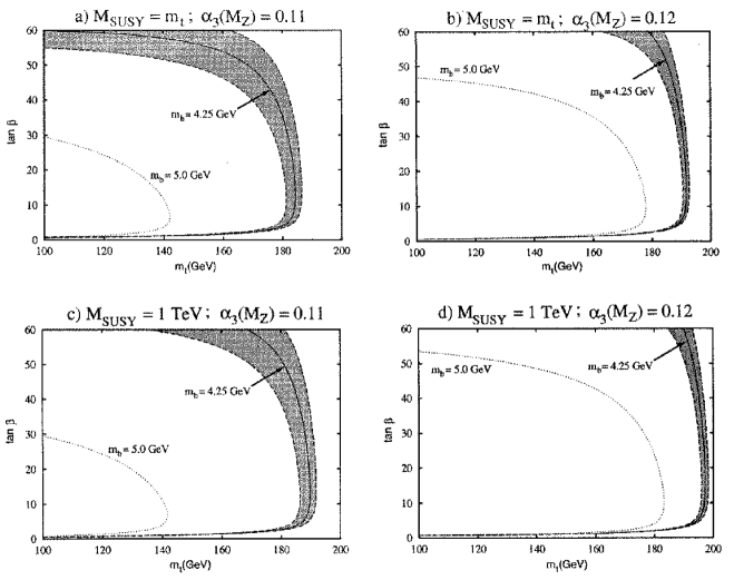
Figure 21: Contours of constant $m_{b}$ in the $\tan\beta$-$m_{t}$-plane obtained from the RG evolution of the MSSM subject to the tau-bottom Yukawa unification constraint at $M_{{\rm GUT}}$ for the parameters a) $M_{{\rm SUSY}}$=$m_{t}$, $\alpha_{s}(m_{Z})=0.11$, b) $M_{{\rm SUSY}}$=$m_{t}$, $\alpha_{s}(m_{Z})=0.12$, c) $\mbox{$M_{{\rm SUSY}}$}=1\,{\rm TeV}$, $\alpha_{s}(m_{Z})=0.11$, d) $\mbox{$M_{{\rm SUSY}}$}=1\,{\rm TeV}$, $\alpha_{s}(m_{Z})=0.12$. The top mass shown is the $\overline{\rm MS}$ mass $m_{t}$; the curves experience a shift of $5\%$ towards higher values if plotted against $m_{t}^{{\rm pole}}$. With this shift the contours appear to lie in the close vicinity of the IR fixed line shown in Fig. 16. The figure was taken from Ref. [55].

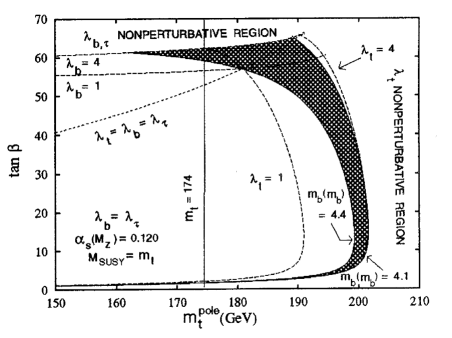
Figure 22: An update of Fig. 21 for $M_{{\rm SUSY}}$=$m_{t}$ and $\alpha_{s}(m_{Z})=0.12$ with $m_{t}$ replaced by $m_{t}^{{\rm pole}}$. Also shown is the line which results from tau-bottom-top Yukawa unification at $M_{{\rm GUT}}$. The contours appear to lie in the close vicinity of the IR fixed line, the IR result of tau-bottom-top Yukawa unification in the close vicinity of the fixed point shown in Fig. 16. The figure was taken from Ref. [63].

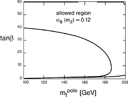
Figure 23: The region in the $\tan\beta$-$m_{t}^{{\rm pole}}$-plane which is consistent with tau-bottom Yukawa unification and with the constraint (245) on the bottom mass for $\alpha_{s}(m_{Z})=0.12$. This figure is adapted from Ref. [58].

Several interesting lessons can be learnt from the whole discussion.

• The very existence of the IR fixed point in $h_{t}$ and, more generally, of the IR fixed line in the $h_{t}$-$h_{b}$ plane, which are inherently to a large extent independent of the UV initial values at $\mu=\mbox{$M_{{\rm GUT}}$}$ of $h_{t}$, resp. of $h_{t}$ and $h_{b}$, provide the basis for being able to accommodate tau-bottom unification and the physical tau and bottom masses simultaneously. Formulated more pointedly, their function is twofold: they implement highly acceptable top mass values and their independence of the UV initial value allows to accommodate the experimental bottom and top masses as well as tau-bottom Yukawa unification. Seen from the gauge and Yukawa unification point of view, the presence of the IR fixed point and line is a very fortunate circumstance.

• As we have seen, the supersymmetric grand unification scenario with tau-bottom Yukawa unification enforces rather large initial values for $h_{t}$($M_{{\rm GUT}}$) or for $h_{b}$($M_{{\rm GUT}}$). These are exactly the initial values for solutions of the RGE which are drawn safely onto the IR fixed point for small $h_{b}$($M_{{\rm GUT}}$), resp. the IR fixed line in the $\tan\beta$-$m_{t}^{{\rm pole}}$-plane. It is for small initial values that the RGE solutions fail to end up in the IR fixed point or line, even given the long evolution path from $M_{{\rm GUT}}$ to $m_{t}$. Thus, seen from the IR physics point of view, the tau-bottom Yukawa unification preselects by a symmetry principle at $M_{{\rm GUT}}$ a portion of the “top-down” RG flow which focuses at the IR scale in the IR fixed manifolds. This is again a very gratifying circumstance.

• The IR physics in the top-bottom sector of a supersymmetric grand unification scenario is to a rather high degree independent of the details of the theory around and above the unification scale $M_{{\rm GUT}}$. What matters for the IR physics is the specific form of the RGE, which had been chosen to be those of the MSSM, and the long evolution path for the RGE flow from a very high UV scale $\Lambda$=$M_{{\rm GUT}}$.

In summary, there is an amazing conspiracy between the ultraviolet physics issues and IR physics issues at work.

As mentioned already there is a large body of interesting papers [50]-[65]in the framework of supersymmetric grand unification, usually adorned with tau-bottom Yukawa unification

• which explore larger grand unifying groups or

• which include all quarks and leptons and their mixing parameters into the numerical analysis or

• all physical Higgs bosons in the two-Higgs sector of the MSSM or

• a realistic spectrum of supersymmetric partners of the ordinary particles or

• radiative electroweak symmetry breaking or

• search for IR fixed points in the supersymmetry breaking mass terms or

• investigation of the IR fixed point structure of the underlying grand unifying gauge theory

Their discussion goes beyond the scope of this review. The qualitative conclusions about the IR fixed point for $m_{t}$, resp. the dependence of the top mass on $\tan\beta$, persist. There are of course changes on the quantitative level.

A very interesting question is: which is the extent of the loss of memory of UV physics at the IR scale. This can be “measured” by varying the physics at the UV scale and evaluating the effect of this variation in the top-bottom sector of the MSSM at the IR scale as e.g. proposed and analysed in Ref. [65]. Similar investigations [118],[119] were performed in the framework of reduction of parameters to be discussed in the next section. The top mass IR fixed point turns out to be remarkably stable towards such variations.

8 Program of Reduction of Parameters

The program of reduction of parameters was formulated quite generally [110]-[112] for renormalizable field theories with more than one coupling. It goes beyond the framework of this review to summarize the full content of the program [110]-[119] including all the recent developments [118],[119]; after some introduction we shall mainly confine the discussion to its application to the SM and occasionally to the MSSM. This restriction will, unfortunately, not allow to do full justice to the scope and beauty of the approach. What will emerge, however, is that the program, starting with the very first publications [110]-[112] already as a systematic search for special solutions of the RGE, has had an effect as role model for the search for IR attractive fixed manifolds, reported on in previous sections, with which it is interrelated to a certain extent.

Starting point of the reduction program is a renormalizable field theory with a set of $n+1$ couplings $\mbox{$\lambda$}_{i}(\mu)$ for $i=1,...,n$ and $g(\mu)$; generically $g$ is an asymptotically free (gauge) coupling. The running of these couplings as functions of the scale parameter $\mu$ is controlled by the perturbative renormalization group equations, $n+1$ coupled non-linear differential equations for these couplings.

The complete reduction program amounts to [110]-[112], [119] a systematic search for special solutions of these RGE

• which establish renormalization group invariant relations between all couplings in the form $\mbox{$\lambda$}_{i}=\mbox{$\lambda$}_{i}(g)$; this requirement is shown to imply the relations between the $\beta$ functions $\beta_{\mbox{$\lambda$}_{i}}={\rm d\,}\mbox{$\lambda$}_{i}/{\rm d\,}\ln(\mu)$ and $\beta_{g}={\rm d\,}g/{\rm d\,}\ln(\mu)$

  $$\beta_{g}\frac{{\rm d\,}\mbox{$\lambda$}_{i}}{{\rm d\,}g}=\beta_{\mbox{$\lambda$}_{i}}\ \ \ {\rm for}\ \ \ i=1,...,n$$ (246)

• and which are not determined by initial value conditions but

• rather by the theoretically appealing boundary condition that with the coupling $g$ also the couplings $\mbox{$\lambda$}_{i}$ vanish, i.e. become asymptotically free in the UV limit $\mu\rightarrow\infty$

  $$\mbox{$\lambda$}_{i}\rightarrow 0\hskip 28.45274pt{\rm for}\hskip 28.45274ptg\rightarrow 0.$$ (247)

In the most restricted form, the dependent couplings $\mbox{$\lambda$}_{i}(g)$ emerge as expansions in powers of $g$, typically in the form

$$\mbox{$\lambda$}_{i}^{2}(g)=\rho_{1i}\,g^{2}+\rho_{2i}\,g^{4}+\rho_{3i}\,g^{6}+...$$ (248)

with constants $\rho_{1i},\ \rho_{2i},...$; less restricted forms allow the expansions also to contain fractional powers or logarithms of $g$. The reduction is called non-trivial, if all the first order coefficients $\rho_{1i}$ in the expansion (248) are positive, trivial if they are zero or, more generally, if $\mbox{$\lambda$}_{i}^{2}/g^{2}\rightarrow 0$ for $g\rightarrow 0$; of course there are also mixed modes of partly nontrivial and partly trivial expansions possible; for a comprehensive recent discussion see Ref. [119].

In any case, complete reduction amounts to reducing the number $n+1$ of independent couplings to a single one, $g$. Provided a reduction is complete, it allows in principle a reduction to all orders in perturbation theory and in practice to the order to which the RGE have been calculated.

It is instructive to relate the result of this program to a general search for IR fixed points, lines, surfaces of the RGE as advocated in earlier sections. A complete non-trivial reduction of the type (248) with positive constants $\rho_{1i}$ amounts at the one-loop level to determining [111] an IR attractive i.e. IR stable fixed point $\mbox{$\lambda$}_{i}^{2}/g^{2}=\rho_{1i}$ for $i=1,...,n$ of the one-loop RGE in the space of the ratios of couplings $\mbox{$\lambda$}_{i}/g$. In the framework of reduction of parameters, this point has the interpretation as an UV repulsive i.e. UV unstable fixed point solution, it exists as such in principle to all orders of perturbation theory, more precisely the existence of a renormalization group trajectory that asymptotically approaches the point in the UV limit is ensured. Despite this vicinity to the search for IR fixed manifolds at the one-loop level, the important difference to this search lies in the selection criterion: instead of selecting special solutions which are IR attractive for the whole RG flow, special solutions are singled out which link all couplings in such a way that they decrease to zero simultaneously in the UV limit $\mu\rightarrow\infty$.

In the application of the program of reduction of parameters to the SM [38],[39] the “driving” coupling $g$ is identified with the strong gauge coupling $g_{3}$; the condition (247) then implies the physical condition that as many couplings of the SM as possible are linked in a renormalization group invariant manner to $g_{3}$ such as to share its property of asymptotic freedom in the UV limit $\mu\rightarrow\infty$. A complete reduction fails in the sector of gauge couplings $g_{1}$, $g_{2}$ and $g_{3}$. The $U(1)$ gauge coupling $g_{1}$ being not asymptotically free also prohibits the performance of the formal limit $\mu\rightarrow\infty$, but rather limits the final analysis to within a finite interval below a physical UV scale $\Lambda$, introduced already in the introduction.

A partial reduction can be performed nevertheless. The analysis [38],[39] of the partial reduction program in the matter sector of the SM then proceeds in a two-step process: in a first step the electroweak gauge couplings are switched off, $g_{1}$=$g_{2}$=0; in a second step the electroweak interactions are systematically and consistently included as corrections in form of a double power series expansion in the ratios $\rho_{1}$=$g_{1}^{2}$/$g_{3}^{2}$and $\rho_{2}$=$g_{2}^{2}$/$g_{3}^{2}$. As results at the bottom line of the analyses [38],[39] are two solutions, a non-trivial one and a trivial one.

Let us start with the non-trivial solution. In the absence of electroweak couplings a consistent and physically meaningful non-trivial solution is found in the top-Higgs-$g_{3}$ sector; at one loop it is identical [111] with the IR attractive fixed point by Pendleton and Ross [30], Eq. (174), in the variables $\rho_{t}$=$g_{t}^{2}$/$g_{3}^{2}$ and $\rho_{H}$=$\lambda$/$g_{3}^{2}$

$$\mbox{$g_{t}^{2}$}=\frac{2}{9}\,\mbox{$g_{3}^{2}$},\hskip 28.45274pt\mbox{$\lambda$}=\frac{\sqrt{689}-25}{72}\,\mbox{$g_{3}^{2}$},$$ (249)

at the two-loop level it is given [113],[114] by the expansion in powers of $g_{3}^{2}$

$$g_{t}^{2} = \frac{2}{9}\,\mbox{$g_{3}^{2}$}+\frac{31359+41\sqrt{689}}{15552}\,\frac{\mbox{$g_{3}$}^{4}}{16\pi^{2}}+...,$$

$$\lambda = \frac{\sqrt{689}-25}{72}\,\mbox{$g_{3}^{2}$}+\frac{147015115-535843\sqrt{689}}{3856896}\,\frac{\mbox{$g_{3}$}^{4}}{16\pi^{2}}+....$$ (250)

At the one-loop level the electroweak couplings are included [39] as perturbations for small values of the ratios $\rho_{1}$=$g_{1}^{2}$/$g_{3}^{2}$ and $\rho_{2}$=$g_{2}^{2}$/$g_{3}^{2}$ in form of a double power series expansion in powers of $\rho_{1}$ and $\rho_{2}$ into the ansatz for a special solution of the RGE for sufficiently small values for $\rho_{1}$ and $\rho_{2}$, subject to the boundary condition that for $\mbox{$\rho_{1}$},\mbox{$\rho_{2}$}\rightarrow 0$ the unperturbed solution (249) is recovered; the result is

$$\mbox{$\rho_{t}$}=\mbox{$g_{t}^{2}$}/\mbox{$g_{3}^{2}$} = \frac{2}{9}-\frac{17}{540}\,\mbox{$\rho_{1}$}-\frac{1}{12}\,\mbox{$\rho_{2}$}+\frac{799}{64800}\,\mbox{$\rho_{1}$}^{2}+\frac{119}{9360}\,\mbox{$\rho_{1}$}\mbox{$\rho_{2}$}-\frac{1}{288}\,\mbox{$\rho_{2}$}^{2}+...$$ (251)

$$\mbox{$\rho_{H}$}=\mbox{$\lambda$}/\mbox{$g_{3}^{2}$} = \frac{\sqrt{689}-25}{72}-\frac{83\sqrt{689}-1295}{66960}\,\mbox{$\rho_{1}$}-\frac{7\sqrt{689}-163}{1488}\,\mbox{$\rho_{2}$}+....$$ (252)

This expansion has a finite radius of convergence in $\rho_{1}$ and $\rho_{2}$ around $\rho_{1}$=$\rho_{2}$=0, but the solution may be extended beyond it numerically.

It is interesting to translate the one-loop result (251) into the language of IR attractive manifolds: it constitutes an IR attractive fixed surface in the three-dimensional $\rho_{t}$-$\rho_{1}$-$\rho_{2}$- space which attracts the “top-down” RG flow very weakly. This can be seen by solving [117] the linearized version of the RGE (209) and around the common IR attractive fixed point $\rho_{t}$=2/9 and $\rho_{1}$=$\rho_{2}$=0, for $\rho_{b}$=$\rho_{\tau}$=0; it has the IR fixed solution (251) with only the linear terms in $\rho_{1}$ and $\rho_{2}$ present. The general solution to this linearized problem can also be obtained [117]; it shows that the IR attractive fixed surface (251) attracts the “top-down” RG flow in the vicinity of the IR fixed point $\rho_{t}$=2/9, $\rho_{1}$=$\rho_{2}$=0 with the small power $(\mbox{$g_{3}^{2}$})^{-1/7}$, i.e. exceedingly weakly. This surface had not been discussed in Sect. 5.1, since it loses the competition with the much stronger IR attractive fixed surface, given in form of analytic expansions in Eqs. (5.1), (221) and numerically in Fig. 10. This may be seen most transparently by following Ref. [39] and Sect. 5.1, i.e. by introducing the experimental initial values for $\mbox{$g_{1}$}(m_{Z})$ and $\mbox{$g_{2}$}(m_{Z})$. This allows to express $\rho_{1}$ and $\rho_{2}$ as functions of 1/$g_{3}^{2}$, and plot the resulting projection of the two surfaces into the $\rho_{t}$-1/$g_{3}^{2}$ plane. The resulting two IR attractive fixed lines are displayed in Fig. 12. The “top-down” RG flow may be read off from Fig. 11; clearly the fat line 1, representing the more attractive fixed line discussed in Sect. 5.1, is much more strongly attractive than the thin line 2, representing the projection of the solution (251) emerging from the one-loop reduction program.

The conclusions arrived at in the last paragraph are important for the search for IR attractive manifolds where the rate of IR attraction counts, while it carries little weight for the parameter reduction approach which is dictated by the boundary condition of asymptotic freedom in the UV limit. In any case the discussion has exhibited yet another interrelation between IR motivated and UV motivated physics issues.

The inclusion of $\rho_{1}$ and $\rho_{2}$ into the solutions (251) and (252) in form of a double power series in powers of $\rho_{1}$ and $\rho_{2}$ cannot be extended, even not in principle, to the UV limit $\mu\rightarrow\infty$, since $\rho_{1}$ will eventually become large and run out of the region of validity of perturbation theory. Thus, in a way, the parameter reduction scheme faces in application to the SM a similar problem as the search for IR attractive fixed manifolds: the increase of $\rho_{1}$ for increasing $\mu$ prevents the former from reaching the mathematical UV limit $\mu\rightarrow\infty$, while the increase of $g_{3}^{2}$ for decreasing $\mu$ prevents the latter from reaching the mathematical IR limit $\mu\rightarrow 0$ [115]. Both approaches have to make do with a finite interval between the IR scale $\mu\simeq\mbox{$m_{t}$}$ and an UV scale $\mbox{$\Lambda$}\mbox{\,\raisebox{1.29167pt}{$<$}$\!\!\!\!\!$\raisebox{-3.87495pt}{$\sim$}\,}10^{19}\mbox{$\,{{\rm GeV}}$}$.

The top and Higgs mass values determined from the one-loop results [39] by evaluating $\rho_{t}$ and $\rho_{H}$ at $\mu=m_{Z}$ are of the order of $\mbox{$m_{t}$}\simeq 91.3\mbox{$\,{{\rm GeV}}$}$ and $\mbox{$m_{H}$}\simeq 64.4\mbox{$\,{{\rm GeV}}$}$. More precise values emerge from the two-loop approach to be presented next. Even though the resulting top mass value is excluded meanwhile by experiment, the discussion provides a welcome deeper insight into the parameter reduction method on a higher loop level.

At the two-loop level [113],[114] besides an expansion in powers of $\rho_{1}$ and $\rho_{2}$ also an expansion in powers of the small parameter $\rho_{b}$=$g_{b}^{2}$/$g_{3}^{2}$ is included. Eqs. (251) and (252) are then replaced by

$$\rho_{t} = \frac{2}{9}-\frac{17}{540}\,\mbox{$\rho_{1}$}-\frac{1}{12}\,\mbox{$\rho_{2}$}-\frac{1}{5}\,\mbox{$\rho_{b}$}+\frac{799}{64800}\,\mbox{$\rho_{1}$}^{2}+\frac{119}{9360}\,\mbox{$\rho_{1}$}\mbox{$\rho_{2}$}-\frac{1}{288}\,\mbox{$\rho_{2}$}^{2}+\frac{9}{400}\,\mbox{$\rho_{1}$}\mbox{$\rho_{b}$}-\frac{54}{175}\,\mbox{$\rho_{b}$}^{2}$$

$$-\frac{5593}{972000}\,\mbox{$\rho_{1}$}^{3}-\frac{323}{62400}\,\mbox{$\rho_{1}$}^{2}\mbox{$\rho_{2}$}+\frac{17}{56160}\,\mbox{$\rho_{1}$}\mbox{$\rho_{2}$}^{2}-\frac{1}{1728}\,\mbox{$\rho_{2}$}^{3}-0.009\,\mbox{$\rho_{1}$}^{2}\mbox{$\rho_{b}$}-0.001\,\mbox{$\rho_{1}$}\mbox{$\rho_{2}$}\mbox{$\rho_{b}$}$$

$$+0.0029\,\mbox{$\rho_{1}$}^{4}+0.0025\,\mbox{$\rho_{1}$}^{3}\mbox{$\rho_{2}$}-0.00008\,\mbox{$\rho_{1}$}^{2}\mbox{$\rho_{2}$}^{2}+0.00005\,\mbox{$\rho_{1}$}\mbox{$\rho_{2}$}^{3}-0.00014\,\mbox{$\rho_{2}$}^{4}+...$$

$$+\frac{\mbox{$g_{3}^{2}$}}{4\pi^{2}}(\frac{31359+41\sqrt{689}}{62208}-0.2231\,\mbox{$\rho_{1}$}-0.8262\,\mbox{$\rho_{2}$}+0.1690\,\mbox{$\rho_{1}$}^{2}+0.1824\,\mbox{$\rho_{1}$}\mbox{$\rho_{2}$}$$

$$-0.0664\,\mbox{$\rho_{2}$}^{2}+...)+...$$

$$\rho_{H} = \frac{\sqrt{689}-25}{72}-\frac{83\sqrt{689}-1295}{66960}\,\mbox{$\rho_{1}$}-\frac{7\sqrt{689}-163}{1488}\,\mbox{$\rho_{2}$}-0.037161\,\mbox{$\rho_{b}$}$$ (253)

$$+.022843\,\mbox{$\rho_{1}$}^{2}+0.0531783\,\mbox{$\rho_{1}$}\mbox{$\rho_{2}$}+0.1092913\,\mbox{$\rho_{2}$}^{2}+0.0362\,\mbox{$\rho_{1}$}\mbox{$\rho_{b}$}+0.024\,\mbox{$\rho_{2}$}\mbox{$\rho_{b}$}$$

$$+0.2725\,\mbox{$\rho_{b}$}^{2}-0.01722\,\mbox{$\rho_{1}$}^{3}-0.032795\,\mbox{$\rho_{1}$}^{2}\mbox{$\rho_{2}$}-0.02158\,\mbox{$\rho_{1}$}\mbox{$\rho_{2}$}^{2}+0.00885\,\mbox{$\rho_{2}$}^{3}$$

$$-0.0160\,\mbox{$\rho_{1}$}^{2}\mbox{$\rho_{b}$}+0.0215\,\mbox{$\rho_{1}$}\mbox{$\rho_{2}$}\mbox{$\rho_{b}$}+0.09348\,\mbox{$\rho_{2}$}^{2}\mbox{$\rho_{b}$}$$

$$+0.0124\,\mbox{$\rho_{1}$}^{4}+0.0226\,\mbox{$\rho_{1}$}^{3}\mbox{$\rho_{2}$}+0.0152\,\mbox{$\rho_{1}$}^{2}\mbox{$\rho_{2}$}^{2}+0.00588\,\mbox{$\rho_{1}$}\mbox{$\rho_{2}$}^{3}+0.00923\,\mbox{$\rho_{2}$}^{4}+...$$

$$\frac{\mbox{$g_{3}^{2}$}}{4\pi^{2}}(\frac{14701515-535843\sqrt{689}}{15427584}-0.03088\,\mbox{$\rho_{1}$}-0.1205\,\mbox{$\rho_{2}$}$$

$$+0.0835\,\mbox{$\rho_{1}$}^{2}-0.0115\,\mbox{$\rho_{1}$}\mbox{$\rho_{2}$}-0.00083\,\mbox{$\rho_{2}$}^{2}+...)+...$$

where the decimal numbers are numerical approximations.

Including a physical value for the bottom mass (5$\,{{\rm GeV}}$), radiative corrections relating the pole masses for the top quark and the Higgs boson to their $\overline{{\rm MS}}$ masses at $\mu=m_{Z}$ the two-loop results lead to the following pole masses [113]

$$\mbox{$m_{t}^{{\rm pole}}$}=99.2\pm 5.7\mbox{$\,{{\rm GeV}}$}\hskip 28.45274pt{\rm and}\hskip 28.45274pt\mbox{$m_{H}^{{\rm pole}}$}=64.6\pm 0.9\mbox{$\,{{\rm GeV}}$}.$$ (254)

The predicted top mass is too low to be compatible with the experimental value.

It is interesting to ask whether the analogous parameter reduction analysis leads to a success in the framework of the MSSM. The answer is no [117]. The one-loop result in absence of the electroweak gauge couplings is identical with the IR attractive fixed point solution (212) a la Pendleton and Ross, the one-loop expansion of $\rho_{t}$ in powers of $\rho_{1}$ and $\rho_{2}$ leads to an IR attractive fixed surface in the $\rho_{t}$-$\rho_{1}$-$\rho_{2}$-space [117] which is again less strongly IR attractive as the one (Fig 10) discussed in Sect. 5.1. Introducing the experimental initial conditions for $\rho_{1}$ and $\rho_{2}$, leads to the solution drawn by the thin line 2 in Fig. 12, which is clearly less strongly attractive than the one drawn by a fat line 1 representing the solution discussed in Sect. 5.1.

The “trivial” solution of the parameter reduction program applied to the SM leads to even smaller top and Higgs masses. There are, however, again very interesting cross relations to the search for IR attractive manifolds at the one-loop level. The one-loop trivial solution [39] in absence of electroweak couplings

$$\mbox{$\rho_{H}$}=\frac{1}{3}\,\mbox{$\rho_{t}$}^{2}+\frac{1}{10}\,\mbox{$\rho_{t}$}^{3}+...$$ (255)

establishes a relation between the ratios of couplings $\rho_{H}$ and $\rho_{t}$. It turns out to be identical with the expansion (180) of the IR attractive fixed line in the $\rho_{t}$-$\rho_{H}$-plane around $\rho_{t}$=$\rho_{H}$=0 (remembering that $R=\mbox{$\rho_{H}$}/\mbox{$\rho_{t}$}$). This solution extends up to the IR fixed point at $\rho_{t}$=2/9, i.e. is historically a precursor of the low $\rho_{t}$ end of the fixed line shown in Fig. 5. The corresponding one-loop expansion including the electroweak corrections [39] is

$$\rho_{H} = \frac{1}{3}\,\mbox{$\rho_{t}$}^{2}+\frac{1}{10}\,\mbox{$\rho_{t}$}^{3}$$ (256)

$$+\frac{27}{2800}\,\mbox{$\rho_{1}$}^{2}(1+\mbox{$\rho_{t}$})+\frac{9}{280}\,\mbox{$\rho_{1}$}\mbox{$\rho_{2}$}(1+\mbox{$\rho_{t}$})+\frac{9}{112}\,\mbox{$\rho_{2}$}^{2}(1+\mbox{$\rho_{t}$})$$

$$-\frac{351}{56000}\,\mbox{$\rho_{1}$}^{3}-\frac{1143}{78400}\,\mbox{$\rho_{1}$}^{2}\mbox{$\rho_{2}$}-\frac{129}{15680}\,\mbox{$\rho_{1}$}\mbox{$\rho_{2}$}^{2}+\frac{33}{3136}\,\mbox{$\rho_{2}$}^{3}-\frac{2}{15}\,\mbox{$\rho_{1}$}\mbox{$\rho_{t}$}^{2}+....$$

Again this is the expansion of the corresponding three-dimensional IR attractive fixed manifold in the $\rho_{t}$-$\rho_{H}$-$\rho_{1}$-$\rho_{2}$-space, discussed in Sect. 4.6 (for $g_{b}$=0), around $\rho_{t}$=$\rho_{H}$=$\rho_{1}$=$\rho_{2}$=0.

In a number of recent interesting publications [118],[119] the program of reduction of parameters is applied to supersymmetric grand unified theories for scales $\mu\geq\mbox{$M_{{\rm GUT}}$}$ above the grand unification scale $M_{{\rm GUT}}$. The advantage is that theories can be singled out which allow a complete reduction. The details of the applications go clearly beyond this review, however, some of the conclusions are very pertinent.

The resulting RG invariant relations between the gauge coupling(s) and the Yukawa couplings for $\mu\geq\mbox{$M_{{\rm GUT}}$}$ are summarized under the headline “gauge-Yukawa unification”. There are typically several physically appealing solutions to each discussed theory, each one providing RG invariant relations between all dimensionless coupling parameters. Generically the UV initial value for the top Yukawa coupling is sufficiently large; in many cases the bottom Yukawa coupling is of the order of the top coupling. The authors [118],[119] then explore the corresponding strongly constrained “top-down” RG flows from $M_{{\rm GUT}}$ to the IR scale $m_{t}$ according to the RGE of the MSSM with $M_{{\rm SUSY}}$ varying within reasonable bounds. Here their various solutions for various theories are caught to a certain extent in the trap of the strongly IR attractive fixed manifolds and and in particular of the IR fixed point for the top mass discussed in Sects. 5 and 6. Thus, in zeroth approximation one expects the IR results to be rather independent of the UV input. The authors work out to which extent the results vary for the different theories and for the different solutions within a given theory. Their top masses lie around 190$\,{{\rm GeV}}$, as expected, with a variation of at most 10$\,{{\rm GeV}}$ from one model or solution to another one; the values for $\tan\beta$ are around 63, signalling top-bottom unification, see Sects. 5.2 and 6.

These gauge-Yukawa reduction scenarios have two features in common with supersymmetric grand unification with tau-bottom Yukawa unification discussed in Sect. 7.

• The top-bottom sector of the IR region is a rather insensitive testing ground for the details of the theory around and above $\mu=\mbox{$M_{{\rm GUT}}$}$.

• The dynamics at the UV scale $M_{{\rm GUT}}$ singles out largish values for the UV initial values for the top and generically also for the bottom Yukawa coupling. This in turn selects that portion of the “top-down” RG flow which is contracted fully onto the IR fixed point in $h_{t}$, resp. on the IR fixed line in the $h_{t}$-$h_{b}$ plane. This enhances strongly the significance of these IR fixed manifolds.

9 Conclusions

The efforts to trace a possible dynamical origin for the top and Higgs masses at the level of the quantum effects, as encoded in the RGE, have been reviewed. The SM and the MSSM have been considered in parallel.

The most important answers to this question lie in IR attractive fixed lines and fixed points which are approached by the “top-down” RG flow from an UV scale $\Lambda$ to the IR scale O$(v)$

• in the $\tan\beta$-$m_{t}^{{\rm pole}}$-plane of the MSSM:

  • for small bottom Yukawa couplings the much quoted very strongly IR attractive fixed point for the top mass

    $$\mbox{$m_{t}^{{\rm pole}}$}=O(190-200)\mbox{$\,{{\rm GeV}}$}\sin\beta$$ (257)

    which is resolved into

    $${\rm a\ genuine\ IR\ fixed\ point\ at}\hskip 14.22636pt\mbox{$m_{t}^{{\rm pole}}$} \approx 190\mbox{$\,{{\rm GeV}}$}\sin\beta,$$ (258)

    $${\rm and\ an\ upper\ bound,\ the\ IR\ image\ of\ large}\hskip 19.91692pt\ \ \ \ \$$

    $${\rm UV\ initial\ values\ for\ the\ top\ Yukawa\ coupling}\hskip 14.22636pt\mbox{$m_{t}^{{\rm pole}}$} \approx 200\mbox{$\,{{\rm GeV}}$}\sin\beta.$$ (259)

  • for unconstrained bottom Yukawa couplings a very strongly IR attractive fixed line in the $\tan\beta$-$m_{t}^{{\rm pole}}$-plane, Fig. 16, with an IR attractive fixed point at

    $$\mbox{$m_{t}^{{\rm pole}}$}\approx 182\mbox{$\,{{\rm GeV}}$},\hskip 28.45274pt\mbox{$\tan\beta$}\approx 60,$$ (260)

    implying approximate bottom-top Yukawa unification.

• in the $m_{H}^{{\rm pole}}$-$m_{t}^{{\rm pole}}$-plane of the SM:

  • a weakly IR attractive fixed point at

    $$\mbox{$m_{t}^{{\rm pole}}$}\approx 214\mbox{$\,{{\rm GeV}}$},\hskip 17.07182pt\mbox{$m_{H}^{{\rm pole}}$}\approx 210\mbox{$\,{{\rm GeV}}$},$$ (261)

  • lying on a strongly attractive IR fixed line in the $m_{H}^{{\rm pole}}$-$m_{t}^{{\rm pole}}$-plane, Fig. 17,

    $${\rm which\ implies}\ \ \ \mbox{$m_{H}^{{\rm pole}}$}\approx 156\mbox{$\,{{\rm GeV}}$}\ \ \ {\rm for}\ \ \ \mbox{$m_{t}^{{\rm pole}}$}=176\mbox{$\,{{\rm GeV}}$}.$$ (262)

As it turns out, the IR attractive top and Higgs mass values are roughly of the order of the electroweak scale, $v/\sqrt{2}$, much larger than the masses of all other matter particles. In particular in the MSSM the resulting top mass $\mbox{$m_{t}^{{\rm pole}}$}=O(190-200)\mbox{$\,{{\rm GeV}}$}\sin\beta$ is well compatible with the experimental value, but also the corresponding SM value $\mbox{$m_{t}$}\approx 215\mbox{$\,{{\rm GeV}}$}$ is not very far from it. This is altogether a very striking result. Of course, as we knew from the outset, in order to judge the significance of these results for physical reality, one needs further experimental information. The MSSM needs an experimental support for the supersymmetry content and an experimental value for $\tan\beta$, the SM as well as the MSSM await the experimental detection of the Higgs boson.

An intricate interrelation between UV physics and IR physics in the MSSM, which has received much attention in the literature, may be summarized as follows.

• The UV symmetry constraint of tau-bottom Yukawa coupling unification in supersymmetric grand unification focuses the RG flow towards the IR scale much more strongly into the IR fixed point top mass value, more precisely onto the IR fixed line in the $\tan\beta$-$m_{t}^{{\rm pole}}$-plane, than the unconstrained RG flow.

• It appears to be the very presence of the IR fixed point in the top mass, resp. of the IR fixed line in the $\tan\beta$-$m_{t}^{{\rm pole}}$-plane, which allows to implement tau-bottom Yukawa unification at the UV scale as well as the physical values of the tau and bottom masses.

• Bottom-top Yukawa unification, a symmetry property at the unification scale in (supersymmetric) grand unification, is also an IR attractive property.

Much effort has been spent in this review to work out the underlying IR fixed manifolds (fixed points, lines, surfaces,…) in the space of ratios of parameters. When all gauge couplings are included, the relevant space is the space of variables $g_{t}^{2}$/$g_{3}^{2}$, $g_{b}^{2}$/$g_{3}^{2}$, $g_{1}^{2}$/$g_{3}^{2}$, $g_{2}^{2}$/$g_{3}^{2}$, treated absolutely in parallel for the SM and the MSSM; in case of the SM the space is further increased by the variable $\lambda$/$g_{3}^{2}$. These higher dimensional manifolds appear to be essential for an insight into the IR fixed points and lines in presence of all gauge couplings. The results are summarized in a compact form in table 2 in Sect. 3. A second important issue was to assess the respective rates of approach towards the various IR attractive manifolds as far as possible analytically. From this collective investigation the following hierarchies emerge.

• The SM and the MSSM have a very similar IR fixed manifold structure. However, the IR attraction for the “top-down” RG flow is systematically stronger in the MSSM than in the SM.

• Generically nontrivial higher dimensional IR attractive manifolds are more strongly IR attractive than the lower dimensional ones.

This last statement needs qualification: In the high dimensional multiparameter space an IR attractive fixed point generically lies at the intersection of two IR attractive lines. Unless accidentally the strength of attraction is equal for both lines, it is always one of the two lines which attracts more strongly. The lines in turn are intersections of two IR attractive surfaces, one of which will be more attractive, etc. The point is that most of these lines and surfaces are trivial ones, e.g. in the sense that they correspond to one variable held constant. It turns out that typically the most non-trivial lines, surfaces, etc. turn out to be the most attractive ones, leading to non-trivial IR attractive relations between the considered parameters.

The triviality and vacuum stability bounds on the SM Higgs mass provide a measure for the distance of the boundaries of the “top-down” RG flow from the IR fixed point and fixed line in the $m_{H}^{{\rm pole}}$-$m_{t}^{{\rm pole}}$-plane as a function of the UV scale $\Lambda$. These bounds are also of relevance for future Higgs searches. Therefore, the most recent precise determinations of the vacuum stability bound in the SM as well as of the upper bound on the mass of the lightest Higgs boson in the MSSM have been included in this review.

Let us close with an outlook from two complementary points of view.

One could entertain the “conservative” expectation that IR physics should be largely independent of UV physics. This may be achieved in a renormalizable theory by arranging the parameters to match the IR attractive (i.e. IR stable) fixed points or fixed lines etc. of the RGEs. In this case the UV scale $\Lambda$, at which new physics arises, the details of the new physics as well as the rate of approach towards the IR fixed manifolds, become largely irrelevant. The only input which counts then is the specific form of the RGEs in the vicinity of the IR scale. Seen under this angle, the IR fixed point structures in Eqs. (257)-(262) are a promising starting point. An investigation into IR fixed manifolds in the remaining quark and lepton sector (even if they were to turn out to be only weakly IR attractive) would be a necessary step towards further support of this point of view.

Very interesting issues have recently been raised in the literature [65], [118], [119], which rely very much on an interrelation between new physics at a high UV scale and the known IR physics.

• From our present knowledge it may appear that whichever new physics in supersymmetric grand unification one formulates: as long as the UV initial values of the top Yukawa couplings are fixed by the UV dynamics to be larger than O(1), the RGE evolution will lead into the “trap” of the IR fixed point for the top mass; if the bottom Yukawa coupling is large in addition, one ends up with $\tan\beta$=O(60). The issue is then [65], [118], [119] to investigate, how “stable” this memory loss of UV physics in the top-bottom sector is with respect to “variations” in the new physics sector. First answers [65], [118], [119] indicate that it is remarkably stable.

• A much furtherreaching issue [65] is the question to which extent the quark and lepton masses and mixing angles as well as the soft supersymmetry breaking mass terms are determined in terms of the IR fixed point structure of the theory lying beyond the SM. First answers [65] indicate that the knowledge of the symmetries and multiplet content of the theory beyond the SM is largely sufficient to determine the IR structure and to lead to very promising results in the low energy sector of the theory.

Acknowledgements: One of us (B.S.) is grateful to J.R. Espinosa, G. Isidori, F. Jegerlehner, B. Kniehl, I. Montvay, F. Schrempp, F. Wagner, P. Weisz, W. Zimmermann for valuable communications and/or enlightning discussions. We also thank F. Schrempp for granting the inclusion of some unpublished results, obtained partly by himself, partly in collaboration with one of us (B.S). One of us (B.S.) is grateful to the DESY theory group for the continuous hospitality.

References

- [1] CDF Collaboration, F. Abe et al., Phys. Rev. Lett. 74 (1995) 2626.
- [2] D0 Collaboration, S. Abachi et al., Phys. Rev. Lett. 74 (1995) 2632.
- [3] D. Schaile, in Proc. of the 1994 Int. Conf. on High Energy Physics, ed. P.J.Bussey and I.G. Knowles, London 1994, p. 27.
- [4] J. Gasser and H. Leutwyler, Phys. Rep. 87 (1982) 77.
- [5] Particle Data Group, L. Montanet et al., Phys. Rev. D50 (1994) 1173.
- [6] L.Maiani, G. Parisi and R. Petronzio, Nucl. Phys. B136 (1978) 115.
- [7] N. Cabbibo, L.Maiani, G. Parisi and R. Petronzio, Nucl. Phys. B158 (1979) 295.
- [8] R. Dashen and H. Neuberger, Phys. Rev. Lett. 50 (1983) 1897.
- [9] M.A.B. Beg, C. Panagiotakopoulos and A. Sirlin, Phys. Rev. Lett. 52 (1984) 883.
-
[10]
M. Lindner, Z. f. Physik C31 (1986) 295;
B. Grzadkowski and M. Lindner, Phys. Lett. B178 (1986) 81;
B. Grzadkowski, M. Lindner and S. Theisen, Phys. Lett. B199 (1987) 64. - [11] M. Lindner, M. Sher and H. Zaglauer, Phys. Lett B228 (1989) 139.
- [12] M. Sher, Phys. Rep. 179 (1989), 273.
- [13] M. Sher , Phys. Lett. B317 (1993) 193)159; Addendum ibid. 331 (1994) 448.
- [14] C. Ford, D.R.T. Jones, P.W. Stephenson and M.B. Einhorn, Nucl. Phys. B395 (1993) 17.
- [15] G. Altarelli and G. Isidori, Phys. Lett B337 (1994) 141.
- [16] J.A. Casas, J.R. Espinosa and M. Quiros, Phys. Lett. B324 (1995) 171.
- [17] J.R. Espinosa and M. Quiros, Phys. Lett. B353 (1995) 257.
- [18] Z. Kunszt and W.J. Stirling, Phys. Lett. B262 (1991) 54.
-
[19]
Y. Okada, M. Yamaguchi and T. Yanagida,
Prog. Theor. Phys. 85 (1991) 1;
J. Ellis, G. Rodolfi and F. Zwirner, Phys. Lett. B257 (1991) 83; ibid. B262 (1991) 477;
R. Barbieri and M Frigeni, Phys. Lett. B258 (1991) 395;
D. Pierce, A. Papadopoulos and S. Johnson, Phys. Rev. Lett. 68 (1992) 3678. -
[20]
H.E. Haber and R. Hempfling, Phys. Rev. Lett. 66
(1991) 1815;
A. Yamada, Phys. Lett. B263 (1991) 233;
A. Brignole, Phys. Lett. B281 (1992) 284;
P.H. Chankowski, S. Pokorski and J. Rosiek, Phys. Lett. B274 (1992) 191. -
[21]
Y. Okada, M. Yamaguchi and T. Yanagida, Phys. Lett. B262 (1991) 54;
R. Barbieri, M. Frigeni and F. Caravaglios, Phys. Lett. B258 (1991) 167;
H. Haber and R. Hempfling, Phys. Rev. D48 (1993) 4280. - [22] J.R. Espinosa and M. Quiros, Phys. Lett. B266 (1991) 389.
- [23] B. Kastening, Phys. Lett. B283 (1992) 287.
- [24] M. Bando, T. Kugo, N. Maekawa and H. Nakano, Phys. Lett. B301 (1993) 83.
- [25] , J. Kodaira, Y. Yasui and K. Sasaki, Phys. Rev. D50 (1994) 7035.
- [26] R. Hempfling and A.H. Hoang, Phys. Lett. B331 (1994) 99.
- [27] J.A. Casas, J.R. Espinosa, M. Quiros and A. Riotto, Nucl. Phys. B436 (1994) 3; Erratum ibid. B439 (1995) 466.
- [28] M. Carena, J.R. Espinosa, M. Quiros and C.E.M. Wagner, Phys. Lett. B355 (1995) 209.
- [29] C.D. Frogatt and H.B. Nielsen, Nucl. Phys. B147 (1979) 277.
- [30] B. Pendleton and G.G. Ross, Phys. Lett. B98 (1981) 291.
- [31] C.T. Hill, Phys. Rev. D24 (1981) 691.
- [32] C. Wetterich, Phys. Lett. 104B (1981) 269.
-
[33]
E. Paschos, Z. Phys. C26 (1984) 235;
J.W. Halley, E. Paschos and H. Usler, Phys. Lett. B155 (1985) 107. - [34] J. Bagger, S. Dimopoulos and E. Masso, Nucl. Phys. B253 (1985) 397.
- [35] S. Dimopoulos and S. Theodorakis, Phys. Lett. 154B (1985) 153.
-
[36]
J. Bagger, S. Dimopoulos and E. Masso, Phys. Lett. B156 (1985) 357;
J. Bagger, S. Dimopoulos and E. Masso, Phys. Rev. Lett. 55 (1985) 1450. - [37] C.T. Hill, C.N. Leung and S. Rao, Nucl. Phys. B262 (1985) 517.
-
[38]
J. Kubo, K. Sibold and W. Zimmermann, Nucl. Phys.
B259 (1985) 331;
K. Sibold and W. Zimmermann, Phys. Lett. B191 (1987) 427.
J. Kubo, K. Sibold and W. Zimmermann, Phys. Lett B220 (1989) 191. - [39] J. Kubo, K. Sibold and W. Zimmermann, Phys. Lett. B220 (1989) 185.
- [40] C. Wetterich, Proc. Trieste HEP Workshop (1987) p.403, and preprint DESY-87-154 (1987).
- [41] C.D. Frogatt, R.G. Moorhouse, Phys. Lett. B249 (1990) 273.
- [42] B. Schrempp and F. Schrempp, Phys. Lett. B299 (1993) 321.
- [43] L. Alvarez Gaume, J. Polchinski and M.B. Wise, Nucl. Phys. B221 (1983) 495.
- [44] J. Bagger, S. Dimopoulos and E. Masso, Phys. Rev. Lett. 55 (1985) 920.
- [45] M. Carena, T.E. Clark, C.E.M. Wagner, W.A. Bardeen and K. Sasaki, Nucl. Phys. B369 (1992) 33.
- [46] C.D. Frogatt, I.G. Knowles and R.G. Moorhouse, Phys. Lett. B298 (1993) 356.
- [47] B. Schrempp, Phys. Lett. 344 (1995) 193.
- [48] B. Schrempp and M. Wimmer, to be published.
- [49] M.S. Chanowitz, J. Ellis and M.K. Gaillard, Nucl. Phys. B128 (1977) 506.
-
[50]
L.E. Ibanez and C. Lopez, Phys.
Lett B126 (1983) 54; Nucl. Phys. B233 (1984) 511;
B. Ananthanarayan, G. Lazarides and Q. Shafi, Phys. Rev. D44 (1991) 1613;
M. Bando, T. Kugo, N. Maekawa and H. Nakano, Mod. Phys. Lett. A7 (1992) 3379;
A. Giveon, L.J. Hall and U. Sarid, Phys. Lett. B271 (1991) 138H. Arason, D.J. Castelano, B. Keszthelyi, S. Mikaelian, E.J. Piard, P. Ramond and B.D. Wright, Phys. Rev. Lett. 67 (1991) 2933 and Phys. Rev. D46 (1992) 3945;
H. Arason, D.J. Castelano, E.J. Piard and P. Ramond, Phys. Rev. D47 (1993) 232;
S. Kelley, J.L. Lopez and D.V. Nanopoulos, Phys. Lett. B274 (1992) 387 and Phys. Lett. B278 (1992) 140;
J. Ellis, S. Kelley and D.V. Nanopoulos, Nucl. Phys. B373 (1992) 55;
G.F. Giudice, Mod. Phys. Lett. A7 (1992) 2429. - [51] G.G. Ross and R.G. Roberts, Nucl. Phys. B377 (1992),571.
- [52] S. Dimopoulos, L. Hall and S. Raby, Phys. Rev. Lett. 68 (1992) 1984.
- [53] S. Dimopoulos, L. Hall and S. Raby , Phys. Rev. D45 (1992) 4192.
- [54] V. Barger, M.S. Berger, T. Han and M. Zralek, Phys. Rev. Lett. 68 (1992) 3394.
- [55] V. Barger, M.S. Berger and P. Ohmann, Phys. Rev. D47 (1993) 1093.
- [56] G. Anderson, S. Dimopoulos, L.J. Hall and S. Raby, Phys. Rev. D47 (1993) 3072.
-
[57]
M. Carena, S. Pokorski and C.E.M. Wagner, Nucl. Phys. B406 (1993) 59;
M. Olechowski and S. Pokorski, Nucl. Phys. B404 (1990) 590;
W. Bardeen, M. Carena, S. Pokorski and C.E.M. Wagner, Phys. Lett. B320 (1994) 110;
M. Carena, L. Clavelli, D. Matalliotakis, H.P. Nilles and C.E.M. Wagner, Phys. Lett. B317 (1993) 346. - [58] P. Langacker and N. Polonsky, Phys. Rev. D49 (1994) 1454.
-
[59]
V. Barger, M.S. Berger, P.
Ohmann and R.J.N. Phillips, Phys. Lett. B314 (1993) 351;
V. Barger, M.S. Berger and P. Ohmann, Phys. Lett. B314 (1993) 351. - [60] B.C. Allanach and S.F. King, Phys. Lett. B328 (1994) 360.
- [61] P. Langacker and N. Polonsky, Phys. Rev. D50 (1994) 2199.
- [62] V. Barger, M.S. Berger and P. Ohmann, Phys. Rev D49 (1994) 4908.
- [63] V. Barger, M.S. Berger and P. Ohmann, Proc. High Energy Physics Conf., Glasgow (1994) Vol.2, 563.
-
[64]
M. Carena, M. Olechowski, S. Pokorski
and C.E.M. Wagner, Nucl. Phys. B419 (1994) 213 and Nucl. Phys.
BB426 (1994) 269;
M. Carena and C.E.M. Wagner, Nucl. Phys. B452 (1995) 45. -
[65]
M. Lanzagorta and G.G. Ross, Phys.
Lett. B349 (1995) 319;
M. Lanzagorta and G.G. Ross, Phys. Lett. B364 (1995)163;
G.G. Ross, Phys. Lett. B364 (1995)216. -
[66]
S.L. Glashow, Nucl. Phys. B22 (1961) 579;
S. Weinberg, Phys. Rev. Lett. 19 (1967) 1264;
A. Salam, in Elementary Particle Theory, N. Svartholm, eds. Amquist and Wiksells, Stockholm (1969) p.376. -
[67]
H. Fritzsch, M. Gell-Mann, H.
Leutwyler, Phys Lett. 47 (1973) 365;
H.D. Politzer, Phys. Rev. Lett. 30 (1973) 1346;
D. Gross, F. Wilczek, Phys. Rev. Lett. 30 (1973) 1343;
S. Weinberg, Phys. Rev. Lett. 31 (1973) 494. - [68] J. Bagger and J. Wess, Introduction to Supersymmetry, Princeton Univ. Press, Princeton NJ (1983).
- [69] H.P. Nilles, Phys. Rep. 110 (1984) 1.
- [70] J.F. Gunion, H.E. Haber, G. Kane and S. Dawson, The Higgs Hunter’s Guide, Addison-Wesley Publishing Company 1990.
- [71] S. Bertolini, F. Borzumati, A. Masiero and G. Ridolfi, Nucl. Phys. B353 (1991) 591.
-
[72]
P. Langacker an M. Luo, Phys. Rev. D44
(1991) 817;
R. Barbieri and L.J. Hall, Phys. Rev. Lett. 68 (1992) 752;
K. Hagiwara and Y. Yamada, Phys. Rev. Lett. 70 (1993) 709;
P. Langacker and N. Polonsky, Phys. Rev. D47 (1993) 4028;
M. Carena, M. Olechowski, S. Pokorski and C.E.M. Wagner, Nucl. Phys. B406 (1993) 59. - [73] P. Langacker and N. Polonsky, Phys. Rev. D47 (1993) 4028.
- [74] P. Langacker and N. Polonsky, Phys. Rev. D52 (1995) 3081.
-
[75]
H. Georgi and S. Glashow, Phys. Rev. Lett. 32 (1974)
438;
H. Georgi, H. Quinn and S. Weinberg, Phys. Rev. Lett. 33 (1974) 451. -
[76]
S. Dimopoulos, S. Raby and F. Wilczek, Phys.
Rev. D24 (1981) 1681;
S. Dimopoulos, and H. Georgi, Nucl. Phys. B193 (1981) 150;
N. Sakai, Zeitschr. f. Phys. C11 (1981) 153;
E. Witten, Nucl. Phys. B188 (1981) 513;
W.J. Marciano and G. Senjanovic, Phys. Rev. D24 (1982) 3092;
L.E. Ibanez and G.G. Ross, Phys. Lett. B105 (1982) 439;
M.B. Einhorn and D.R.T. Jones, Nucl. Phys. B196 (1982) 439. -
[77]
G.G. Ross, Grand Unified Theories, Benjamin/Cummings, New York, 1984;
R.N. Mohapatra, Unification and Supersymmetry, Sringer, New York, 1992. -
[78]
U. Amaldi, W. de Boer and H. Fürstenau, Phys. Lett. B260 (1991) 447;
J. Ellis, S. Kelley and D.V. Nanopoulos, Phys. Lett. B249 (1990) 441;
P. Langacker and M. Luo, Phys. Rev. D44 (1991) 817;
F. Anselmo, L. Cifarelli, A. Peterman and A. Zichichi, Nuovo Cimento A104 (1991) 1817. -
[79]
M.E. Machacek and Vaughn, Nucl. Phys B222 (1983)
83; ibid. B236 (1984) 221; ibid. B249 (1985) 70;
M. Fischler and J. Oliensis, Phys. Lett. B119 (1982) 385; Phys. Rev. D28 (1983) 2027;
I. Jack, J. Phys. A16 (1983) 1083;
I. Jack and H. Osborn, ibid. A16 (1983) 1101;
I. Jack, Phys. Lett. B147 (1984) 405;
I. Jack and H. Osborn, Nucl. Phys. B249 (1985) 472;
C. Ford, I. Jack and D.R.T. Jones, Rep. No. NSF-ITP-92-21 (1992);
C. Ford, D.R.T. Jones, P.W. Stephenson and M.B. Einhorn, Nucl. Phys. B395 (1993) 17. -
[80]
K. Inoue, A. Kakuto and S. Takeshita, Prog. Theor.
Phys. 67 (1982) 1889; ibid. 68 (1982) 927;
D.R.T. Jones and L.Mezincescu, Phys. Lett. B136 (1984) 242;
P. West, Phys. Lett. B137 (1984) 371;
A. Parkes and P. West, Phys. Lett. B138 (1984) 99;
D.R.T. Jones and L. Mezinescu, Phys. Lett B138 (1984) 293;
M.E.Machacek and M.T. Vaughn, Nucl. Phys. B236 (1984) 221;
J.P. Derendinger and C.A. Savoy, Nucl. Phys. B237 (1984) 307;
B. Gato, J. Leon, J. Perez-Mercader and M. Quiros, Nucl. Phys. B253 285;
N.K. Falk, Zeitschr. f. Phys. C10 (1986) 247. J.E. Björkman and D.R.T. Jones, Nucl. Phys. B259 (1985) 533;
A.J. Parkes, Phys. Lett. B156 (1985) 73;
D.R.T. Jones and A.J. Parkes, Phys. Lett. B160 (1985)267;
S.P. Martin and M.T. Vaughn, Phys. Rev. D50 (1994) 2282. -
[81]
S. Willenbrock and G. Valencia, Phys. Lett. B259
(1991) 373;
R.G. Stuart, Phys. Lett B262 (1991) 113; ibid. B272 (1991) 353; Phys. Rev. Lett. 70 (1993) 3193;
A. Sirlin, Phys. Rev. Lett. 67 (1991) 2127; Phys. Lett. B267 (1991) 240. - [82] R. Tarrach, Nucl. Phys. B183 (1981) 384.
-
[83]
O.V. Tarasov, A.A. Vladimirov and A.Y Zarkov, Phys.Lett.
93B (1980) 429;
S.G. Gorishny, A.L. Kataev and S.A. Larin, Yad. Fiz. 40 (1984) 517 [Sov. J. Nucl. Phys. 40 (1984) 329];
S.G. Gorishny, A.L. Kataev, S.A. Larin and L.R. Surguladze, Mod. Phys. Lett. A5 (1990) 2703. - [84] N. Gray, D.J. Broadhurst, W. Grafe and K. Schilcher, Zeitschr. Phys. C48 (1990) 673.
- [85] R. Barbieri, M.Beccaria, P. Ciafaloni, G. Curci and A. Vicere, Nucl. Phys. B409 (1993) 105.
- [86] A.I. Bochkarev and R.S. Willey, Phys. Rev. D51 (1995) 2049.
- [87] R. Hempfling and B.A. Kniehl, Phys. Rev D51 (1995) 1386.
- [88] A. Sirlin and R. Zucchini, Nucl. Phys. B266 (1986) 389.
- [89] see e.g. J. Guckenheimer and P. Holmes, Non-linear Oscillations, Dynamical Systems and Bifurcations of Vector Fields, Applg. Math. Sciences, Vol 42, Springer Verlag (1983).
- [90] W. Marciano, Phys. Rev. D29 (1984) 580.
-
[91]
A.A. Vladimirov, D.I. Kazakov and O.V. Tarasov,
Sov. Phys. JETP 50 (1979) 521;
I. Jack and H. Osborn, J. Phys. A16 (1983) 1101. - [92] B.W. Lee, C. Quigg and H. Thacker, Phys. Rev. D16 (1977) 1519.
- [93] W. Marciano, G. Valencia and S. Willenbrock, Phys. Rev. D40 (1989) 1725.
- [94] M. Lüscher and P. Weisz, Phys. Lett. B212 (1988) 472.
- [95] U. Nierste and K. Riesselmann, Technical Univ. Munich preprint TUM-T31-90/95 (1995), hep-ph/9511407.
- [96] S. Cortese, E. Pallante and R. Petronzio, Phys. Lett. B301 (1993) 203.
-
[97]
J. Fröhlich, Nucl. Phys. B100 (1982) 281;
M. Aizenmann, Phys. Rev. Lett. 4̱7 (1981)1;
J. Glimm and A. Jaffe, Ann. Inst. Henri Poincaré 22 (1975) 97. - [98] W.A. Bardeen and M. Moshe, Phys. Rev. D28 (1983) 1372.
- [99] B. Freedman, P. Smolensky and D Weingarten, Phys. Lett. B113 (1982) 481.
- [100] D. Callaway and R. Petronzio, Nucl. Phys. b240 (1984) 577.
-
[101]
M. Lüscher and P. Weisz, Nucl. Phys. 290
(1987) 25;
M. Lüscher and P. Weisz, Nucl. Phys. 295 (1988) 65;
M. Lüscher and P. Weisz, Nucl. Phys. 300 (1988) 353;
M. Lüscher and P. Weisz, Nucl. Phys. B318 (1989) 705. -
[102]
J. Kuti, L. Lin and Y. Shen, Phys. Rev. Lett. 61
(1988) 678;
A. Hasenfratz, K. Jansen, J. Jersak, C.B. Lang, T. Neuhaus and H. Yoneyama, Nucl. Phys. B317 (1989) 81;
G. Bhanot and K. Bitar, Phys. Rev. Lett. 61 (1988) 798;
G. Bhanot, K. Bitar, U.M. Heller and H. Neuberger, Nucl. Phys. B353 (1991) 551 (erratum Nucl. Phys. B375 (1992) 503;
U.M Heller, H. Neuberger and P. Vranas, Nucl. Phys. B399 (1993) 271; Phys. Lett. B238 (1992) 335;
M. Göckeler, H.A. Kastrup, T. Neuhaus and F. Zimmermann, Nucl. Phys. B404 (1993) 517;
U.M. Heller, M. Klomfass, H. Neuberger and P. Vranas, Nucl. Phys. B405 (1993) 555. - [103] for a recent review see e.g. U.M. Heller, Nucl. Phys. B (Proc. Suppl.) (1994) 101.
-
[104]
L. Lin, I. Montvay, G. Münster and H. Wittig, Nucl.
Phys. B355 (1985) 165;
C. Frick, L. Lin, I. Montvay, G. Münster, M. Plagge, T. Trappenberg and H. Wittig, Nucl. Phys. B397 (1993) 431; Nucl. Phys. B (Proc. Suppl.) 30 (1993) 647;
l. Lin and H. Wittig, Z. Phys. C 54 (1992) 331. - [105] L. Lin, I. Montvay, G. Münster, M. Plagge and H. Wittig, Phys. Lett. B317 (1993) 143.
-
[106]
A. Borrelli, L. Maiani, G.C. Rossi, R. Sisto and M.
Testa, Phys. Lett. B221 (1989) 360;
M.F. Goltermann and D.N. Petcher, Phys. Lett. B225 (1989) 159. - [107] W.A. Bardeen, C.T. Hill and M. Lindner, Phys. Rev. D41 (1990) 1647.
- [108] M. Lindner, Int. Jounal of Mod. Phys. A8 (1993) 2176 and references therein.
- [109] B. Schrempp and F. Schrempp (unpublished).
-
[110]
W. Zimmermann, Comm. Math. Phys. 97 (1985) 211;
R. Oehme and W. Zimmermann, Comm. Math. Phys. 97 (1985) 569. - [111] R. Oehme, Progr. Theor. Phys. Suppl. 86 (1985) 215.
- [112] R. Oehme, K. Sibold and W. Zimmermann, Phys. Lett. B153 (1985) 142.
- [113] J. Kubo, Phys. Lett. B262 (1991) 472
- [114] W. Zimmermann, Phys. Lett. B311 (1993) 249.
- [115] W. Zimmermann, Phys. Lett. B308 (1993) 117.
- [116] W. Zimmermann, Lett. Math. Phys. 30 (1994) 61.
- [117] B. Schrempp unpublished.
-
[118]
D. Kapetanakis, M.
Mondragon and G. Zoupanos, Zeitschr. f. Phys. C60 (1993) 181;
M. Mondragon and G. Zoupanos, Nucl. Phys. B (Proc. Suppl.) 37C (1995) 98;
J. Kubo,M. Mondragon, N.D. Tracas and G. Zoupanos, Phys. Lett. B342 (1995) 155. - [119] J. Kubo, M. Mondragon and G. Zoupanos, Nucl. Phys. B424 (1994) 291.