Heavy Quarkonia: Wilson Area Law, Stochastic Vacuum Model and Dual QCD

Abstract

The $Q\bar{Q}$ semirelativistic interaction in QCD can be simply expressed in terms of the Wilson loop and its functional derivatives. In this approach we present the $Q\bar{Q}$ potential up to order $1/m^{2}$ using the expressions for the Wilson loop given by the Wilson Minimal Area Law (MAL), the Stochastic Vacuum Model (SVM) and Dual QCD (DQCD). We confirm the original results given in the different frameworks and obtain new contributions. In particular we calculate up to order $1/m^{2}$ the complete velocity dependent potential in the SVM. This allows us to show that the MAL model is entirely contained in the SVM. We compare and discuss also the SVM and the DQCD potentials. It turns out that in these two very different models the spin-orbit potentials show up the same leading non-perturbative contributions and $1/r$ corrections in the long-range limit.

I INTRODUCTION

Since the pioneering paper of Wilson [1] a real breakthrough opened in the treatment of quark states and in this framework a lot of work was devoted to the study of the heavy $Q\bar{Q}$. The challenge was understanding low energy QCD dynamics and hence confinement. The main characteristics of the heavy meson and baryon spectrum are simple and cleanly connected to expectation value of the $Q\bar{Q}$ and $3Q$ potentials. The size of the $b$ and $c$ systems extends over distances where confinement already plays a relevant role (only toponium can be described purely in terms of one gluon exchange plus higher order perturbative corrections [2] but, as well-known, we cannot access its spectrum); moreover, due to the mean value of the quark velocities, the leading relativistic corrections can be appreciated and usefully tested on the data. Furthermore, a good understanding of the heavy quark semirelativistic interaction is the first step towards relativistic generalization.

At the static level, the linear confining $Q\bar{Q}$ interaction, corresponding to a constant energy density (the string tension $\sigma$) localized in a flux tube between the quarks, emerges in lattice formulation of QCD and is contained in all the existing confining models, e.g., Wilson area law, flux tube model and all kind of dielectric and dual models. This corresponds also to the static limit of the Buchmüller’s picture [3] of a rotating quark-antiquark state connected by a purely chromoelectric tube with a pure transverse velocity and with chromomagnetic field vanishing in the comoving system of the tube. In this picture it follows simply that the non-perturbative spin-interaction is given only by the Thomas precession term.

The spin-dependent relativistic corrections were calculated first by Eichten, Feinberg [4] and Gromes [5] as a correction to the static limit (Wilson–Brown–Weisberger area law result). The potential is expressed in terms of average of electric and magnetic fields that can also be calculated on the lattice. The Eichten–Feinberg–Gromes results, at least in the long range behaviour, have been reproduced on the lattice [6, 7] (for a detailed discussion see Sec. 6). Recently the spin-dependent potential was also studied in the context of the Heavy Quark Effective Theory [8].

In the literature relativistic generalizations of these results were attempted in a Bethe–Salpeter context by constructing a Bethe–Salpeter kernel which give back static and spin-dependent potentials. Using a simple convolution kernel (i.e. depending only on the momentum transfer $Q$), this amounts to considering a Lorentz scalar proportional to $1/Q^{4}$. The velocity dependent relativistic corrections were also obtained but they are strongly dependent on the type of “instantaneous” approximation chosen to define the potential and on the gauge. These non-perturbative velocity dependent corrections destroy the agreement with the data [9, 10, 11] and give origin to the puzzle of how reconciling the spin-structure (i.e. the Lorentz nature of the kernel) with the velocity corrections in one Bethe–Salpeter kernel. In this paper we will not deal with this problem starting directly from the $1/m^{2}$ expansion of the potential without any relativistic assumption. However a first step in its resolution seems to be the correct inclusion of the low energy dynamics also in the spin-independent $1/m^{2}$ corrections. Moreover from the knowledge of these and the spin dependent corrections we will obtain some important insights on the nature of the kernel.

Recently a method to obtain the complete $1/m^{2}$ quark–antiquark (and 3 quarks) potential, based on the path integral representation of the Pauli–type quark propagator, was given in [12] (see also [13, 14] and [15]). This formulation is gauge invariant. The potential is obtained as a function of a generalized Wilson loop (i.e. any kind of trajectory for the quark and the antiquark can appear) and its functional derivatives. These are all measurable on the lattice. In short it was obtained a constituent quark semirelativistic interaction with coefficients determined by the non linear gluodynamics. This is the ideal framework in which to formulate hypothesis on the Wilson loop behaviour (and so on the confinement mechanism) to be checked on the lattice and on the experimental data.

First, to evaluate the non-perturbative behaviour of the Wilson loop, a modified minimal area law (MAL) was used (see Sec. 3). This reproduces the Eichten–Feinberg–Gromes results [4, 5] and gives a velocity dependent potential proportional to the flux tube angular momentum squared, so that, by including velocity dependent corrections, a “string model” emerges (see [11, 16]). Also the velocity dependent potentials seem to agree with recent available lattice data [17].

However, the MAL represents an extreme approximation that gives the correct result for very large interquark distances and does not give insight into open problems such as the relation between the non-perturbative structure of spin and velocity corrections. For these reasons we have taken into account two models of confinement, the stochastic vacuum model (SVM) and Dual QCD (DQCD) which both give an expression for the whole behaviour of the Wilson loop and contain the area law in the long distances limit. It is interesting to realize that both models reproduce essentially the perturbative plus MAL results respectively in the limit of short and long distances but produce also subleading corrections. These allows us to understand better the physical picture. For example in the case of the non-perturbative spin-orbit interaction it turns out that the magnetic term cancels in the area law limit (zero magnetic field in the comoving framework) but presents $1/r$ suppressed corrections in the other two models.

A careful comparison between the SVM and DQCD corrections and an investigation of the approximations in which they coincide seem to be of great importance to the aim of understanding the low energy gluodynamics contained in the Wilson loop.

The plan of the paper is the following one. In Sec. 2 we briefly sum up the definition of the semirelativistic potential and the notations. In Sec. 3 we collect the results obtained in the MAL model. In Sec. 4 we briefly present the SVM and use it to evaluate the potential in the context of Sec. 2. In particular we obtain also the SVM velocity dependent potential which is new. We show that it satisfies important identities and we give the short and long-range limits. In Sec. 5 we introduce the DQCD potential and discuss the long-range limit. In Sec. 6 we discuss our results in connection with the up to now available lattice data and draw some conclusions.

II THE QUARK-ANTIQUARK POTENTIAL

In [12] a Foldy–Wouthuysen transformation on the quark-antiquark Green’s function was done and the result was written as a Feynman path integral over particle and anti-particle coordinates and momenta of a Lagrangian depending only upon the spin, coordinates, and momenta of the quark and antiquark. Separating off the kinetic terms from this Lagrangian it was possible to identify the heavy quark potential $V_{{\rm Q}\bar{\rm Q}}$ (closed loops of light quark pairs and annihilation contributions were not included):

$$\int_{t_{\rm i}}^{t_{\rm f}}dtV_{{\rm Q}\bar{{\rm Q}}} = i\log\langle W(\Gamma)\rangle-\sum_{j=1}^{2}\frac{g}{m_{j}}\int_{{\Gamma}_{j}}dx^{\mu}\left(S_{j}^{l}\,\langle\!\langle\hat{F}_{l\mu}(x)\rangle\!\rangle-\frac{1}{2m_{j}}S_{j}^{l}\varepsilon^{lkr}p_{j}^{k}\,\langle\!\langle F_{\mu r}(x)\rangle\!\rangle\right.$$ (1)

$$\quad\quad-\left.\frac{1}{8m_{j}}\,\langle\!\langle D^{\nu}F_{\nu\mu}(x)\rangle\!\rangle\right)-\frac{1}{2}\sum_{j,j^{\prime}=1}^{2}\frac{ig^{2}}{m_{j}m_{j^{\prime}}}{\rm T_{s}}\int_{{\Gamma}_{j}}dx^{\mu}\,\int_{{\Gamma}_{j^{\prime}}}dx^{\prime\sigma}\,S_{j}^{l}\,S_{j^{\prime}}^{k}$$ (2)

$$\quad\quad\times\left(\,\langle\!\langle\hat{F}_{l\mu}(x)\hat{F}_{k\sigma}(x^{\prime})\rangle\!\rangle-\,\langle\!\langle\hat{F}_{l\mu}(x)\rangle\!\rangle\,\langle\!\langle\hat{F}_{k\sigma}(x^{\prime})\rangle\!\rangle\right)\>,$$ (3)

where

$$F_{\mu\nu} = \partial_{\mu}A_{\nu}-\partial_{\nu}A_{\mu}+ig\,[A_{\mu},A_{\nu}]\,,\quad\quad\quad\hat{F}^{\mu\nu}\equiv{1\over 2}\varepsilon^{\mu\nu\rho\sigma}F_{\rho\sigma}\,,$$ (4)

$$D^{\nu}F_{\nu\mu} = \partial^{\nu}F_{\nu\mu}+ig[A^{\nu},F_{\nu\mu}]\>,$$ (5)

$$W(\Gamma) \equiv {\rm P\>}\exp\left[ig\oint_{\Gamma}dx^{\mu}A_{\mu}(x)\right]\>,$$ (6)

and

$$\langle f(A)\rangle \equiv {1\over 3}{\rm Tr\>}{\rm P\>}{\int{\cal D}A\,e^{iS_{\rm YM}(A)}f(A)\over\int{\cal D}A\,e^{iS_{\rm YM}(A)}}\>,$$ (7)

$$\langle\!\langle f(A)\rangle\!\rangle \equiv {\int{\cal D}A\,e^{iS_{\rm YM}(A)}{\rm Tr\>}{\rm P\>}\{f(A)\exp\left[ig\oint_{\Gamma}dx^{\mu}A_{\mu}(x)\right]\}\over\int{\cal D}A\,e^{iS_{\rm YM}(A)}{\rm Tr\>}{\rm P\>}{\exp\left[ig\oint_{\Gamma}dx^{\mu}A_{\mu}(x)\right]}}\>.$$ (8)

The closed loop $\Gamma$ is defined by the quark (anti-quark) trajectories ${\bf z}_{1}(t)$ (${\bf z}_{2}(t)$) running from ${\bf y}_{1}$ to ${\bf x}_{1}$ (${\bf x}_{2}$ to ${\bf y}_{2}$) as $t$ varies from the initial time $t_{\rm i}$ to the final time $t_{\rm f}$. The quark (anti-quark) trajectories ${\bf z}_{1}(t)$ (${\bf z}_{2}(t)$) define the world lines $\Gamma_{1}$ ($\Gamma_{2}$) running from $t_{\rm i}$ to $t_{\rm f}$ ($t_{\rm f}$ to $t_{\rm i}$). The world lines $\Gamma_{1}$ and $\Gamma_{2}$, along with two straight-lines at fixed time connecting ${\bf y}_{1}$ to ${\bf y}_{2}$ and ${\bf x}_{1}$ to ${\bf x}_{2}$, then make up the contour $\Gamma$ (see Fig. 1). As usual $A_{\mu}(x)\equiv A_{\mu}^{a}(x)\lambda_{a}/2$, ${\rm Tr}$ means the trace over color indices, ${\rm P}$ prescribes the ordering of the color matrices according to the direction fixed on the loop and $S_{\rm YM}(A)$ is the Yang–Mills action including a gauge fixing term.

As the $1/m^{2}$ terms in $V_{{\rm Q}\bar{\rm Q}}$ are of two types, velocity dependent $V_{\rm VD}$ and spin dependent $V_{\rm SD}$, we can identify in the full potential three type of contributions:

$$V_{{\rm Q}\bar{\rm Q}}=V_{0}+V_{\rm VD}+V_{\rm SD}\>,$$ (9)

with $V_{0}$ the static potential.

The spin independent part of the potential, $V_{0}+V_{\rm VD}$, is obtained in (3) from the zero order and the quadratic terms in the expansion of $\log\langle W(\Gamma)\rangle$ for small velocities ${\dot{\bf z}}_{1}(t)={\bf p}_{1}/m_{1}$ and ${\dot{\bf z}}_{2}(t)={\bf p}_{2}/m_{2}$. In the notation of [13, 19] the terms arising from this expansion can be rearranged as:

$$i\log\langle W(\Gamma)\rangle = \int_{t_{i}}^{t_{f}}dt~{}V_{0}(r(t))+V_{\rm VD}({\bf r}(t))\,,$$ (10)

$$V_{\rm VD}({\bf r}(t)) = {1\over m_{1}m_{2}}\left\{{\bf p}_{1}\cdot{\bf p}_{2}V_{\rm b}(r)+\left({1\over 3}{\bf p}_{1}\cdot{\bf p}_{2}-{{\bf p}_{1}\cdot{\bf r}\>~{}{\bf p}_{2}\cdot{\bf r}\over r^{2}}\right)V_{\rm c}(r)\right\}_{\rm Weyl}$$ (11)

$$+ \sum_{j=1}^{2}{1\over m_{j}^{2}}\left\{p^{2}_{j}V_{\rm d}(r)+\left({1\over 3}p^{2}_{j}-{{\bf p}_{j}\cdot{\bf r}\>~{}{\bf p}_{j}\cdot{\bf r}\over r^{2}}\right)V_{\rm e}(r)\right\}_{\rm Weyl}\,,$$ (12)

where ${\bf r}(t)\equiv{\bf z}_{1}(t)-{\bf z}_{2}(t)$ and the symbol $\{\>~{}\}_{\rm Weyl}$ stands for the Weyl ordering prescription among momentum and position variables [12].

The spin dependent potential $V_{\rm SD}$ contains for each quark terms analogous to those obtained by making a Foldy–Wouthuysen transformation on the Dirac equation in an external field (where $\langle\!\langle F_{\mu\nu}\rangle\!\rangle$ plays the role of the external field), along with an additional term $V_{\rm SS}$ having the structure of a spin-spin interaction. We can then write

$$V_{\rm SD}=V_{\rm LS}^{\rm MAG}+V_{\rm Thomas}+V_{\rm Darwin}+V_{\rm SS}\>,$$ (13)

using a notation which indicates the physical significance of the individual terms (MAG denotes Magnetic). The correspondence between (13) and (3) is given by

$$\int_{t_{\rm i}}^{t_{\rm f}}dtV_{\rm LS}^{\rm MAG} = -\sum_{j=1}^{2}\frac{g}{m_{j}}\int_{{\Gamma}_{j}}dx^{\mu}S_{j}^{l}\,\langle\!\langle\hat{F}_{l\mu}(x)\rangle\!\rangle\>,$$ (14)

$$\int_{t_{\rm i}}^{t_{\rm f}}dtV_{\rm Thomas} = \sum_{j=1}^{2}\frac{g}{2m^{2}_{j}}\int_{{\Gamma}_{j}}dx^{\mu}S_{j}^{l}\varepsilon^{lkr}p_{j}^{k}\,\langle\!\langle F_{\mu r}(x)\rangle\!\rangle\>,$$ (15)

$$\int_{t_{\rm i}}^{t_{\rm f}}dtV_{\rm Darwin} = \sum_{j=1}^{2}\frac{g}{8m^{2}_{j}}\int_{{\Gamma}_{j}}dx^{\mu}\langle\!\langle D^{\nu}F_{\nu\mu}(x)\rangle\!\rangle\>,$$ (16)

$$\int_{t_{\rm i}}^{t_{\rm f}}dtV_{\rm SS} = -\frac{1}{2}\sum_{j,j^{\prime}}\frac{ig^{2}}{m_{j}m_{j^{\prime}}}{\rm T_{s}}\int_{{\Gamma}_{j}}dx^{\mu}\,\int_{{\Gamma}_{j^{\prime}}}dx^{\prime\sigma}\,S_{j}^{l}\,S_{j^{\prime}}^{k}\left(\,\langle\!\langle\hat{F}_{l\mu}(x)\hat{F}_{k\sigma}(x^{\prime})\rangle\!\rangle\right.$$ (17)

$$\quad\quad\quad\quad\quad\quad\left.-\langle\!\langle\hat{F}_{l\mu}(x)\rangle\!\rangle\,\langle\!\langle\hat{F}_{k\sigma}(x^{\prime})\rangle\!\rangle\right)\>.$$ (18)

In the well-known Eichten and Feinberg notation [4] and taking also into account the Darwin potential and similar contributions arising from the spin-spin interaction [13, 19], the terms in $V_{\rm SD}$ can be rearranged as

$$V_{\rm SD} = {1\over 8}\left({1\over m_{1}^{2}}+{1\over m_{2}^{2}}\right)\Delta\left[V_{0}(r)+V_{\rm a}(r)\right]$$ (19)

$$+ \left({1\over 2m_{1}^{2}}{\bf L}_{1}\cdot{\bf S}_{1}-{1\over 2m_{2}^{2}}{\bf L}_{2}\cdot{\bf S}_{2}\right){1\over r}{d\over dr}\left[V_{0}(r)+2V_{1}(r)\right]$$ (20)

$$+ {1\over m_{1}m_{2}}\left({\bf L}_{1}\cdot{\bf S}_{2}-{\bf L}_{2}\cdot{\bf S}_{1}\right){1\over r}{d\over dr}V_{2}(r)+{1\over m_{1}m_{2}}\left({{\bf S}_{1}\cdot{\bf r}\>{\bf S}_{2}\cdot{\bf r}\over r^{2}}-{1\over 3}{\bf S}_{1}\cdot{\bf S}_{2}\right)V_{3}(r)$$ (21)

$$+ {1\over 3m_{1}m_{2}}{\bf S}_{1}\cdot{\bf S}_{2}\,V_{4}(r)\>,$$ (22)

with ${\bf L}_{j}={\bf r}\times{\bf p}_{j}$. It is not possible to identify directly each Eichten and Feinberg potential with the terms contained in eq. (3) without making some assumptions on the Wilson loop. This will be the aim of the next sections. But some observations are just now possible. The contributions to $\Delta(V_{0}+V_{\rm a})$ come from $V_{\rm Darwin}$ and from $V_{\rm SS}$ with $j=j^{\prime}$. In the case $j\neq j^{\prime}$, $V_{\rm SS}$ contributes to the tensor term $V_{3}$ and to the spin-spin term $V_{4}$. Finally, $V_{1}$ receives contributions from both the magnetic ($V_{\rm LS}^{\rm MAG}$) and the Thomas precession term ($V_{\rm Thomas}$) while the contributions to $V_{2}$ come only from the magnetic term.

Due to the Lorentz invariance properties of the Wilson loop some exact relations for the potentials $V_{i}$ and $V_{\rm a}$, …, $V_{\rm e}$ can be obtained. The first was given by Gromes [5] for the spin-related potentials

$${d\over dr}\left[V_{0}(r)+V_{1}(r)-V_{2}(r)\right]=0\>,$$ (23)

and the other one by Barchielli, Brambilla and Prosperi [14] for the velocity-related potentials

$$V_{\rm d}(r)+{1\over 2}V_{\rm b}(r)+{1\over 4}V_{0}(r)-{r\over 12}{dV_{0}(r)\over dr}=0\>,$$ (24)

$$V_{\rm e}(r)+{1\over 2}V_{\rm c}(r)+{r\over 4}{dV_{0}(r)\over dr}=0\>.$$ (25)

Since these relations are due to the Lorentz invariance they must be satisfied by any good choice of the Wilson loop approximated behaviour.

Summarizing, the static and velocity dependent part of the potential are given in terms of the expansion of the Wilson loop average $\langle W(\Gamma)\rangle$, while the spin dependent potentials are given as a sum of terms depending upon the quark and antiquark spins, masses and momenta with coefficients which are expectation values of operators computed in presence of a moving quark-antiquark pair. These expectation values can be obtained as functional derivatives of $\log\langle W(\Gamma)\rangle$ with respect to the path, i.e. with respect to the quark trajectories ${\bf z}_{1}(t)$ or ${\bf z}_{2}(t)$. In fact let us consider the change in $\langle W(\Gamma)\rangle$ induced by letting $z_{j}^{\mu}(t)\rightarrow z_{j}^{\mu}(t)+\delta z_{j}^{\mu}(t)$ where $\delta z_{j}^{\mu}(t_{\rm i})=\delta z_{j}^{\mu}(t_{\rm f})=0$:

$$g\langle\!\langle F_{\mu\nu}(z_{j})\rangle\!\rangle=(-1)^{j+1}{\delta i\log\langle W(\Gamma)\rangle\over\delta S^{\mu\nu}(z_{j})}\>,$$ (26)

$$\delta S^{\mu\nu}(z_{j})=(dz_{j}^{\mu}\delta z_{j}^{\nu}-dz_{j}^{\nu}\delta z_{j}^{\mu})\>.$$

Varying again the path

$$g^{2}\left(\langle\!\langle F_{\mu\nu}(z_{1})F_{\lambda\rho}(z_{2})\rangle\!\rangle-\langle\!\langle F_{\mu\nu}(z_{1})\rangle\!\rangle\langle\!\langle F_{\lambda\rho}(z_{2})\rangle\!\rangle\right)=-ig{\delta\over\delta S^{\lambda\rho}(z_{2})}\langle\!\langle F_{\mu\nu}(z_{1})\rangle\!\rangle.$$ (27)

All contributions to the spin dependent part of the potential can be expressed as first and second variational derivatives of $\log\langle W(\Gamma)\rangle$. Therefore the whole quark-antiquark potential depends only on the assumed behaviour of $\langle W(\Gamma)\rangle$. In the next sections we will discuss some of these assumptions and give for each of them the explicit analytical expression of the potential.

III MINIMAL AREA LAW MODEL (MAL)

In Ref. [12, 14] $\langle W(\Gamma)\rangle$ was approximated by the sum of a perturbative part given at the leading order by the gluon propagator $D_{\mu\nu}$ and a non-perturbative part given by the value of the minimal area of the deformed Wilson loop of fixed contour $\Gamma$ plus a perimeter contribution $\cal P$:

$$i\log\langle W(\Gamma)\rangle = i\log\langle W(\Gamma)\rangle^{\rm SR}+i\log\langle W(\Gamma)\rangle^{\rm LR}$$ (28)

$$= -\frac{4}{3}g^{2}\oint_{\Gamma}dx^{\mu}_{1}\oint_{\Gamma}dx^{\nu}_{2}~{}iD_{\mu\nu}(x_{1}-x_{2})+\sigma S_{\rm min}+{C\over 2}{\cal P}\>.$$ (29)

Denoting by $u^{\mu}=u^{\mu}(s,t)$ the equation of any surface with contour $\Gamma$ ($s\in[0,1],\,t\in[t_{\rm i},t_{\rm f}],\,u^{0}(s,t)=t,\,{\bf u}(1,t)={\bf z}_{1}(t),\,{\bf u}(0,t)={\bf z}_{2}(t)\,$) and defining ${\bf u}_{\rm T}\equiv{\bf u}-({\bf u}\cdot{\bf n})~{}{\bf n}$ with ${\bf n}=(\partial{\bf u}/\partial s)|\partial{\bf u}/\partial s|^{-1}$, we can write:

$$S_{\rm min} = \min\int_{t_{\rm i}}^{t_{\rm f}}dt\,\int_{0}^{1}ds\,\left[-\left(\frac{\partial u^{\mu}}{\partial t}\frac{\partial u_{\mu}}{\partial t}\right)\left(\frac{\partial u^{\mu}}{\partial s}\frac{\partial u_{\mu}}{\partial s}\right)+\left(\frac{\partial u^{\mu}}{\partial t}\frac{\partial u_{\mu}}{\partial s}\right)^{2}\right]^{\frac{1}{2}}$$ (30)

$$= \min\int_{t_{\rm i}}^{t_{\rm f}}dt\,\int_{0}^{1}ds\,\left|\frac{\partial{\bf u}}{\partial s}\right|\left\{1-\left[\left(\frac{\partial{\bf u}}{\partial t}\right)_{\rm T}\right]^{2}\right\}^{\frac{1}{2}}\>,$$ (31)

which coincides with the Nambu–Goto action. Up to the order $1/m^{2}$ the minimal surface can be identified exactly (see App. B ref.[12]) with the surface spanned by the straight-line joining $(t,{\bf z}_{1}(t))$ to $(t,{\bf z}_{2}(t))$ with $t_{\rm i}\leq t\leq t_{\rm f}$. The generic point of this surface is

$$u^{0}_{\min}=t\quad\quad\quad{\bf u}_{\min}=s~{}{\bf z}_{1}(t)+(1-s)~{}{\bf z}_{2}(t)\>,$$ (32)

with $0\leq s\leq 1$ and ${\bf z}_{1}(t)$ and ${\bf z}_{2}(t)$ being the positions of the quark and the antiquark at the time $t$. Then, the exact expression for the minimal area at the order $1/m^{2}$ in the MAL turns out to be

$$S_{\min} = \int_{t_{\rm i}}^{t_{\rm f}}dt\,r\int_{0}^{1}ds\,[1-(s~{}\dot{{\bf z}}_{1\rm T}+(1-s)~{}\dot{{\bf z}}_{2\rm T})^{2}]^{\frac{1}{2}}=$$ (33)

$$= \int_{t_{\rm i}}^{t_{\rm f}}dt\,r\,\left[1-\frac{1}{6}\left(\dot{{\bf z}}_{1\rm T}^{2}+\dot{{\bf z}}_{2\rm T}^{2}+\dot{{\bf z}}_{1\rm T}\cdot\dot{{\bf z}}_{2\rm T}\right)+\ldots\,\,\right]\>.$$ (34)

The perimeter term is given simply by

$${\cal P}=|{\bf x}_{1}-{\bf x}_{2}|+|{\bf y}_{1}-{\bf y}_{2}|+\sum_{j=1}^{2}\int_{t_{\rm i}}^{t_{\rm f}}dt\sqrt{\dot{z}_{j}^{\mu}\dot{z}_{j\mu}}\>,$$ (35)

and it is clear that we can neglect the time-independent perimeter contribution to the potential in the limit of big time interval $t_{\rm f}-t_{\rm i}$. By expanding also eq. (35) at the $1/m^{2}$ order we have

$$i\log\langle W(\Gamma)\rangle^{\rm LR}=\int_{t_{\rm i}}^{t_{\rm f}}dt\,\sigma r\,\left[1-\frac{1}{6}\left(\dot{{\bf z}}_{1\rm T}^{2}+\dot{{\bf z}}_{2\rm T}^{2}+\dot{{\bf z}}_{1\rm T}\cdot\dot{{\bf z}}_{2\rm T}\right)\right]+{C\over 2}\sum_{j=1}^{2}\int_{t_{\rm i}}^{t_{\rm f}}dt\left(1-{1\over 2}\dot{z}_{j}^{h}\dot{z}_{j}^{h}\right)\>.$$ (36)

For what concerns the perturbative part in the limit for large $t_{\rm f}-t_{\rm i}$ the only non-vanishing contribution to the Wilson loop is given by

$$i\log\langle W(\Gamma)\rangle^{\rm SR}=-\frac{4}{3}g^{2}\int_{t_{\rm i}}^{t_{\rm f}}dt_{1}\int_{t_{\rm i}}^{t_{\rm f}}dt_{2}~{}{\dot{z}}_{1}^{\mu}(t_{1})~{}{\dot{z}}_{2}^{\nu}(t_{2})~{}iD_{\mu\nu}(z_{1}-z_{2})\>.$$ (37)

In the infinite time limit this expression is still gauge invariant. Expanding $z_{2}(t_{2})$ around $t_{1}$ it is possible to evaluate explicitly from eq. (37) the short-range potential up to a given order in the inverse of the mass. Self-energy terms are neglected.

So, in this framework the following (MAL) static and velocity dependent potential were obtained:

$$V_{0}=-{4\over 3}{\alpha_{\rm s}\over r}+\sigma r+C\>,$$ (38)

and the explicit expressions for the potentials are:

$$V_{\rm b}(r) = {8\over 9}{\alpha_{\rm s}\over r}-{1\over 9}\sigma r\>,\quad\quad\,~{}V_{\rm c}(r)=-{2\over 3}{\alpha_{\rm s}\over r}-{1\over 6}\sigma r\>,$$ (39)

$$V_{\rm d}(r) = -{1\over 9}\sigma r-{1\over 4}C\>,\quad\quad V_{\rm e}(r)=-{1\over 6}\sigma r\>.$$ (40)

These potentials fulfil the exact relations (24) and (25)

Moreover by evaluating the functional derivatives for the Wilson loop, as given by eqs. (26)-(27), we obtain also the spin-dependent potentials

$$\Delta V_{\rm a}(r)=0\>,\quad{d\over dr}V_{1}(r)=-\sigma\>,\quad{d\over dr}V_{2}(r)={4\over 3}{\alpha_{\rm s}\over r^{2}}\>,\quad V_{3}(r)=4{\alpha_{\rm s}\over r^{3}}\>,\quad V_{4}(r)={32\over 3}\pi\alpha_{\rm s}\delta^{3}({\bf r})\>.$$ (41)

These potentials reproduce the Eichten–Feinberg–Gromes results [4] and fulfil the Gromes relation (23). Notice that, as a consequence of the vanishing in this model of the long-range behaviour of the spin-spin potential $V_{\rm SS}$ and the spin-orbit magnetic potential $V_{\rm LS}^{\rm MAG}$, there is no long-range contribution to $V_{2}$, $V_{3}$ and $V_{4}$. Instead $V_{1}$ has only a non-perturbative long-range contribution, which comes from the Thomas precession potential (15).

The MAL model strictly corresponds to the Buchmüller picture [3] where the magnetic field in the comoving system is taken to be equal to zero. Let us first notice that the perimeter contributions at the $1/m^{2}$ order can be simply absorbed in a redefinition of the quark masses $m_{j}\to m_{j}+C/2$ (for details see [14]). Then let us consider the moving quark and antiquark connected by a chromoelectric flux tube and let us describe the flux tube as a string with pure transverse velocity ${\bf v}_{\rm t}$. At the classical relativistic level the system is described by the flux tube Lagrangian [20, 21]

$${\cal L}=-\sum_{j=1}^{2}m_{j}\sqrt{1-{\bf v}_{j}^{2}}-\sigma\int_{0}^{r}dr^{\prime}\sqrt{1-{\bf v}_{\rm t}^{\prime 2}}\>,$$ (42)

with ${\bf v}_{\rm t}^{\prime}={\bf v}_{1{\rm t}}~{}{r^{\prime}/r}+{\bf v}_{2{\rm t}}(1-{r^{\prime}/r})$. The semirelativistic limit of this Lagrangian gives back the non-perturbative part of the $V_{0}$ and $V_{\rm VD}$ potential in the MAL model (notice that the minimal area law in the straight-line approximation is the configuration given by a straight flux tube) . The remarkable characteristics of the obtained $V_{\rm VD}$ potential is the fact that it is proportional to the square of the angular momentum and so takes into account the energy and angular momentum of the string:

$$V_{\rm VD}^{\rm LR}=-{1\over 12m_{1}m_{2}}{\sigma\over r}({\bf L}_{1}\cdot{\bf L}_{2}+{\bf L}_{2}\cdot{\bf L}_{1})-\sum_{j=1}^{2}{1\over 6m_{j}^{2}}{\sigma\over r}{\bf L}_{j}^{2}\>.$$ (43)

Finally, the non-perturbative spin-dependent part of the potential in this intuitive flux tube picture simply comes from the Buchmüller ansatz that the chromomagnetic field is zero in the comoving framework of the flux tube.

We notice that even if $V_{1}$ seems to arise from an effective Bethe–Salpeter kernel which is a scalar and depends only on the momentum transfer, a simple convolution kernel cannot reproduce the correct velocity dependent potential (43) or equivalently (40) [22]. Nevertheless the behaviour (43) seems to be important to reproduce the spectrum [9, 10, 11, 16, 23, 24].

IV STOCHASTIC VACUUM MODEL (SVM)

The SVM (see [15, 25] and for a review [26]) in the context of heavy quark bound state gives a justification of the MAL model avoiding the artificial splitting of the Wilson loop in a perturbative and a non-perturbative part. It reproduces the flux tube distribution measured on the lattice [27]. Moreover it allows to go beyond the MAL model in a systematic way (e.g. with the so-called perturbation theory in non-perturbative background [28]). The whole non-perturbative physics is factorized in some correlation function which can be calculated on the lattice.

The starting point is to express the Wilson loop average $\langle W(\Gamma)\rangle$ via the non-Abelian Stokes theorem [29, 30] in terms of an integral over a surface $S$ enclosed by the contour $\Gamma$, and then to perform a cluster expansion [31]. In order to allow lattice calculations all these quantities are given in the Euclidean metric. Some care must be payed in converting it in the Minkowskian metric before putting in eq. (3).

$$\langle W(\Gamma)\rangle = \left\langle{\rm P}\>\exp\left(ig\int_{S}dS_{\mu\nu}(u)F_{\mu\nu}(u,x_{0})\right)\right\rangle$$ (44)

$$= \exp\sum_{j=1}^{\infty}{(ig)^{j}\over j!}\int_{S}dS_{\mu_{1}\nu_{1}}(u_{1})\dots$$ (45)

$$\quad\quad\quad\int_{S}dS_{\mu_{j}\nu_{j}}(u_{j})\langle F_{\mu_{1}\nu_{1}}(u_{1},x_{0})\dots F_{\mu_{j}\nu_{j}}(u_{j},x_{0})\rangle_{\rm cum}\>.$$ (46)

The cumulants $\langle~{}\>\rangle_{\rm cum}$ are defined in terms of average values over the gauge fields $\langle~{}\>\rangle$:

$$\langle F(1)\rangle_{\rm cum}=\langle F(1)\rangle\>,\quad\quad\langle F(1)F(2)\rangle_{\rm cum}=\langle F(1)F(2)\rangle-\langle F(1)\rangle\langle F(2)\rangle\>,~{}~{}\dots$$ (47)

and ${\rm P\>}F_{\mu,\nu}(u,x_{0})\equiv{\rm P\>}\exp\left[ig\int_{x_{0}}^{u}dx^{\mu}A_{\mu}(x)\right]F_{\mu\nu}(u)\exp\left[ig\int^{x_{0}}_{u}dx^{\mu}A_{\mu}(x)\right]$ where $x_{0}$ is an arbitrary reference point on the surface $S$ appearing in the non-Abelian Stokes theorem (44). In general each cumulant depends on $S$ and on $x_{0}$, but, as the left-hand side of eq. (44) does not, it is expected that in the full resummation of all the cumulants (right-hand side of eq. (46)) this dependence will disappear [30]. To minimize the required cancellations $S$ is chosen to be the minimal area surface.

Equation (46) is exact. The first cumulant vanishes trivially. The second cumulant gives the first non-zero contribution to the cluster expansion (46). In the SVM one assumes that in the context of heavy quark bound states higher cumulants can be neglected and the second cumulant dominates the cluster expansion, or, in other words, that the vacuum fluctuations are of a Gaussian type:

$$\log\langle W(\Gamma)\rangle=-{g^{2}\over 2}\int_{S}dS_{\mu\nu}(u)\int_{S}dS_{\lambda\rho}(v)\langle F_{\mu\nu}(u,x_{0})F_{\lambda\rho}(v,x_{0})\rangle_{\rm cum}\>.$$ (48)

Neglecting the dependence on $x_{0}$ and on the arbitrary curves connecting $x_{0}$ with $u$ and $v$ which seems to be relegated to higher correlators, the Lorentz structure of the bilocal cumulant implies that it can be expressed as [15]:

$$\langle F_{\mu\nu}(u,x_{0})F_{\lambda\rho}(v,x_{0})\rangle_{\rm cum} = \langle F_{\mu\nu}(u,x_{0})F_{\lambda\rho}(v,x_{0})\rangle\>$$ (49)

$$= {\beta\over g^{2}}\Bigg{\{}(\delta_{\mu\lambda}\delta_{\nu\rho}-\delta_{\mu\rho}\delta_{\nu\lambda})D\left((u-v)^{2}\right)$$ (50)

$$+ {1\over 2}\left[{\partial\over\partial u_{\mu}}\left((u-v)_{\lambda}\delta_{\nu\rho}-(u-v)_{\rho}\delta_{\nu\lambda}\right)\right.$$ (51)

$$\quad\quad\quad\left.+{\partial\over\partial u_{\nu}}\left((u-v)_{\rho}\delta_{\mu\lambda}-(u-v)_{\lambda}\delta_{\mu\rho}\right)\right]D_{1}\left((u-v)^{2}\right)\Bigg{\}}$$ (52)

$$\beta \equiv {g^{2}\over 36}{\langle{\rm Tr\>}F_{\mu\nu}(0)F_{\mu\nu}(0)\rangle\over D(0)+D_{1}(0)}\>.$$ (53)

Eq. (48) and (52) define the SVM for heavy quarks. The correlator functions $D$ and $D_{1}$ are unknown. The perturbative part of $D_{1}$, which is expected to be dominant in the short-range behaviour, can be obtained by means of the standard perturbation theory:

$$D_{1}^{\rm pert}(x^{2})={16\alpha_{\rm s}\over 3\pi}{1\over x^{4}}+~{}{\rm higher~{}~{}orders}\>.$$ (54)

Instead the only information which we know about the non-perturbative contributions to $D$ and $D_{1}$ come from lattice simulations. A good parametrization of the long-range behaviour of the bilocal correlators seems to be [32, 33]:

$$\beta~{}D^{\rm LR}(x^{2}) = d~{}e^{-\delta|x|}\>,\quad\>\delta=(1\pm 0.1)~{}{\rm GeV}\>,\quad d=0.073~{}{\rm GeV}^{4}\>,$$ (55)

$$\beta~{}D_{1}^{\rm LR}(x^{2}) = d_{1}~{}e^{-\delta_{1}|x|}\>,\quad\delta_{1}=(1\pm 0.1)~{}{\rm GeV}\>,\quad d_{1}=0.0254~{}{\rm GeV}^{4}\>,$$ (56)

Up to order $1/m^{2}$ the minimal area surface can be identified, as in the previous section, with the straight-line surface (32). In particular, since $dS_{\mu\nu}(u)$ $\equiv$ $dt~{}ds~{}$ $\partial u_{\mu}(t,s)/\partial t~{}~{}$ $\partial u_{\nu}(t,s)/\partial s$, we have:

$$dS_{4j}(u) = dt~{}ds~{}r_{j}(t)\>;$$ (57)

$$dS_{ij}(u) = dt~{}ds~{}\left(s~{}{\dot{z}}_{i1}(t)+(1-s)~{}{\dot{z}}_{i2}(t)\right)~{}r_{j}(t)\>.$$ (58)

From (48) and (52) and taking in account (32) we have calculated explicitly $\log\langle W(\Gamma)\rangle$. Considering time interval much larger than the typical correlation length of $D$ and $D_{1}$, up to order $1/m^{2}$ we have (for details see the appendix):

$$V_{0}(r) = \beta\int_{-\infty}^{+\infty}d\tau\left\{\int_{0}^{r}d\lambda(r-\lambda)~{}D(\tau^{2}+\lambda^{2})+\int_{0}^{r}d\lambda{\lambda\over 2}D_{1}(\tau^{2}+\lambda^{2})\right\}\>,$$ (59)

$$V_{\rm b}(r) = {\beta\over 6}\int_{-\infty}^{+\infty}d\tau\left\{\int_{0}^{r}d\lambda\left(-{2\over 3}r-{\lambda^{2}\over r}+{8\over 3}{\lambda^{3}\over r^{2}}-3{\tau^{2}\over r}\right)~{}D(\tau^{2}+\lambda^{2})\right.$$ (60)

$$\quad\quad\left.+\int_{0}^{r}d\lambda\left(-{3\over 2}{\lambda^{2}\over r}+{3\over 2}{\tau^{2}\over r}\right)D_{1}(\tau^{2}+\lambda^{2})+{r^{2}\over 2}D_{1}(\tau^{2}+r^{2})\right\}\>,$$ (61)

$$V_{\rm c}(r) = {\beta\over 2}\int_{-\infty}^{+\infty}d\tau\left\{\int_{0}^{r}d\lambda\left(-{r\over 3}-2{\lambda^{2}\over r}+{4\over 3}{\lambda^{3}\over r^{2}}\right)~{}D(\tau^{2}+\lambda^{2})\right.$$ (62)

$$\quad\quad\left.-{r^{2}\over 2}D_{1}(\tau^{2}+r^{2})\right\}\>,$$ (63)

$$V_{\rm d}(r) = {\beta\over 6}\int_{-\infty}^{+\infty}d\tau\left\{\int_{0}^{r}d\lambda\left(-{2\over 3}r+{3\over 2}\lambda+{1\over 2}{\lambda^{2}\over r}-{4\over 3}{\lambda^{3}\over r^{2}}+{3\over 2}{\tau^{2}\over r}\right)~{}D(\tau^{2}+\lambda^{2})\right.$$ (64)

$$\quad\quad\left.+\int_{0}^{r}d\lambda\left(-{3\over 4}\lambda+{3\over 4}{\lambda^{2}\over r}-{3\over 4}{\tau^{2}\over r}\right)D_{1}(\tau^{2}+\lambda^{2})\right\}\>,$$ (65)

$$V_{\rm e}(r) = {\beta\over 2}\int_{-\infty}^{+\infty}d\tau\int_{0}^{r}d\lambda\left(-{r\over 3}+{\lambda^{2}\over r}-{2\over 3}{\lambda^{3}\over r^{2}}\right)~{}D(\tau^{2}+\lambda^{2})\>.$$ (66)

Result (59) was found in [15], whereas (61)-(66) are new. We note that these expressions for the potentials $V_{0}$ and $V_{\rm b}$, …, $V_{\rm e}$ satisfy identically the Barchielli–Brambilla–Prosperi relations (24) and (25). Of particular interest seems to be the potential $V_{\rm e}$ that has only non-perturbative contributions in the bilocal approximation.

To evaluate the spin dependent part of the potential, the only terms which we need are those with one and two field strength insertions (taking in account that $\langle\!\langle D^{\nu}F_{\nu\mu}(x)\rangle\!\rangle=\partial_{\nu}\langle\!\langle F_{\nu\mu}(x)\rangle\!\rangle$). By means of eq. (26) and (27) and (48):

$$g\langle\!\langle F_{0l}(z_{j})\rangle\!\rangle = \beta r_{l}\int_{-\infty}^{+\infty}d\tau\left\{\int_{0}^{r}d\lambda{1\over r}D(\tau^{2}+\lambda^{2})+{1\over 2}D_{1}(\tau^{2}+r^{2})\right\}\>,$$ (67)

$$g\langle\!\langle F_{il}(z_{1})\rangle\!\rangle = \beta\left({\dot{z}}_{l1}r_{i}-{\dot{z}}_{i1}r_{l}\right)\int_{-\infty}^{+\infty}d\tau\int_{0}^{r}d\lambda{1\over r}\left(1-{\lambda\over r}\right)D(\tau^{2}+\lambda^{2})$$ (68)

$$+ \beta\left({\dot{z}}_{l2}r_{i}-{\dot{z}}_{i2}r_{l}\right)\int_{-\infty}^{+\infty}d\tau\left\{\int_{0}^{r}d\lambda{\lambda\over r^{2}}D(\tau^{2}+\lambda^{2})+{1\over 2}D_{1}(\tau^{2}+r^{2})\right\}\>,$$ (69)

$$g\langle\!\langle F_{il}(z_{2})\rangle\!\rangle = \beta\left({\dot{z}}_{l2}r_{i}-{\dot{z}}_{i2}r_{l}\right)\int_{-\infty}^{+\infty}d\tau\int_{0}^{r}d\lambda{1\over r}\left(1-{\lambda\over r}\right)D(\tau^{2}+\lambda^{2})$$ (70)

$$+ \beta\left({\dot{z}}_{l1}r_{i}-{\dot{z}}_{i1}r_{l}\right)\int_{-\infty}^{+\infty}d\tau\left\{\int_{0}^{r}d\lambda{\lambda\over r^{2}}D(\tau^{2}+\lambda^{2})+{1\over 2}D_{1}(\tau^{2}+r^{2})\right\}\>,$$ (71)

$$g^{2}\left(\langle\!\langle F_{\mu\nu}(z_{1})F_{\lambda\rho}(z_{2})\rangle\!\rangle-\langle\!\langle F_{\mu\nu}(z_{1})\rangle\!\rangle\langle\!\langle F_{\lambda\rho}(z_{2})\rangle\!\rangle\right)=\quad\quad\quad\quad\quad\quad\quad\quad\quad$$ (72)

$$\quad\quad\quad\quad\quad\beta(\delta_{\mu\lambda}\delta_{\nu\rho}-\delta_{\mu\rho}\delta_{\nu\lambda})\left(D(\tau^{2}+r^{2})+D_{1}(\tau^{2}+r^{2})\right)$$ (73)

$$\quad\quad\quad\quad+\beta\left(r_{\mu}r_{\lambda}\delta_{\nu\rho}-r_{\mu}r_{\rho}\delta_{\nu\lambda}+r_{\nu}r_{\rho}\delta_{\mu\lambda}-r_{\nu}r_{\lambda}\delta_{\mu\rho}\right){\partial\over\partial\tau^{2}}D_{1}(\tau^{2}+r^{2})\>,\quad\quad r_{4}\equiv\tau=t_{1}-t_{2}\>.$$ (74)

In this way we obtain the following expressions for the spin-dependent potentials in the SVM (confirming the results obtained in [15] with a different derivation):

$$\Delta V_{\rm a}(r) = {\hbox{self-energy terms}}\>,$$ (75)

$${d\over dr}V_{1}(r) = -\beta\int_{-\infty}^{+\infty}d\tau\int_{0}^{r}d\lambda\left(1-{\lambda\over r}\right)~{}D(\tau^{2}+\lambda^{2})\>,$$ (76)

$${d\over dr}V_{2}(r) = \beta\int_{-\infty}^{+\infty}d\tau\left\{\int_{0}^{r}d\lambda{\lambda\over r}~{}D(\tau^{2}+\lambda^{2})+{1\over 2}rD_{1}(\tau^{2}+r^{2})\right\}\>,$$ (77)

$$V_{3}(r) = -\beta\int_{-\infty}^{+\infty}d\tau~{}r^{2}{\partial\over\partial\tau^{2}}D_{1}(\tau^{2}+r^{2})\>,$$ (78)

$$V_{4}(r) = \beta\int_{-\infty}^{+\infty}d\tau~{}\left\{3D(\tau^{2}+r^{2})+3D_{1}(\tau^{2}+r^{2})+2r^{2}{\partial\over\partial\tau^{2}}D_{1}(\tau^{2}+r^{2})\right\}\>.$$ (79)

Potentials (59), (76) and (77) satisfy identically the Gromes relation (23). An application of the spin potentials to the $b\bar{b}$ and $c\bar{c}$ spectrum, with a discussion on the different type of parametrization of the correlation functions, can be found in [33, 34].

In the short-range behaviour ($r\to 0$), assuming that all the relevant contributions come from the perturbative part of $D_{1}$ (54) eqs.(59)-(66) and (76)-(75) exactly reproduce (after subtracting the self-energy contributions) the $\alpha_{\rm s}$-depending part of eqs. (38), (40) and (41) of the MAL model. We observe that no gauge choice is necessary in this approach, which is manifestly gauge-invariant. Moreover we note that the short-range behaviour of the $D_{1}$ correlator is not ad hoc but emerges straightforwardly from the comparison with the $\alpha_{\rm s}$ expansion of the Wilson loop.

In the long-range behaviour ($r\to\infty$):

$$V_{0}(r)=\sigma_{2}r+{1\over 2}C_{2}^{(1)}-C_{2}\>,\quad{d\over dr}V_{1}(r)=-\sigma_{2}+{C_{2}\over r}\>,\quad{d\over dr}V_{2}(r)={C_{2}\over r}\>,$$ (80)

$V_{3}$ and $V_{4}$ fall off exponentially and

$$\Delta V_{\rm a}(r) = {\hbox{self-energy terms}}\>,$$ (81)

$$V_{\rm b}(r) = -{1\over 9}\sigma_{2}r-{2\over 3}{D_{2}\over r}+{8\over 3}{E_{2}\over r^{2}}\>,\quad\quad\quad\quad\quad\quad\quad\>~{}V_{\rm c}(r)=-{1\over 6}\sigma_{2}r-{D_{2}\over r}+{2\over 3}{E_{2}\over r^{2}}\>,$$ (82)

$$V_{\rm d}(r) = -{1\over 9}\sigma_{2}r+{1\over 4}C_{2}-{1\over 8}C_{2}^{(1)}+{1\over 3}{D_{2}\over r}-{2\over 9}{E_{2}\over r^{2}}\>,\quad V_{\rm e}(r)=-{1\over 6}\sigma_{2}r+{1\over 2}{D_{2}\over r}-{1\over 3}{E_{2}\over r^{2}}\>,$$ (83)

with

$$\sigma_{2} \equiv \beta\int_{-\infty}^{+\infty}d\tau\int_{0}^{\infty}d\lambda~{}D(\tau^{2}+\lambda^{2})\>,$$ (84)

$$C_{2} \equiv \beta\int_{-\infty}^{+\infty}d\tau\int_{0}^{\infty}d\lambda~{}\lambda~{}D(\tau^{2}+\lambda^{2})\>,\quad\quad~{}C_{2}^{(1)}\equiv\beta\int_{-\infty}^{+\infty}d\tau\int_{0}^{\infty}d\lambda~{}\lambda~{}D_{1}(\tau^{2}+\lambda^{2})\>,$$ (85)

$$D_{2} \equiv \beta\int_{-\infty}^{+\infty}d\tau\int_{0}^{\infty}d\lambda~{}\lambda^{2}~{}D(\tau^{2}+\lambda^{2})\>,$$ (86)

$$E_{2} \equiv \beta\int_{-\infty}^{+\infty}d\tau\int_{0}^{\infty}d\lambda~{}\lambda^{3}~{}D(\tau^{2}+\lambda^{2})\>.$$ (87)

By means of parametrization (55)-(56) we have

$$\sigma_{2} = {\pi d\over\delta^{2}}\simeq 0.2~{}{\rm GeV^{2}}\>,\quad C_{2}={4d\over\delta^{3}}\simeq 0.3~{}{\rm GeV}\>,$$ (88)

$$C_{2}^{(1)} = {4d_{1}\over\delta_{1}^{2}}\simeq 0.1~{}{\rm GeV}\>,\quad D_{2}={3\pi d\over\delta^{4}}\simeq 0.7\>,\quad\>E_{2}={32d\over\delta^{5}}\simeq 2.3~{}{\rm GeV}^{-1}\>,$$ (89)

and

$$V_{3}(r) = 1.2(6)~{}d_{1}\sqrt{\delta_{1}}~{}r^{3\over 2}e^{-\delta_{1}r}\>,$$ (90)

$$V_{4}(r) = 1.2(6)~{}{6d\over\sqrt{\delta}}~{}r^{1\over 2}e^{-\delta r}+1.2(6)~{}{6d_{1}\over\sqrt{\delta_{1}}}~{}r^{1\over 2}e^{-\delta_{1}r}-2.5(2)~{}d_{1}\sqrt{\delta_{1}}~{}r^{3\over 2}e^{-\delta_{1}r}\>.$$ (91)

Identifying $\sigma_{2}$ with $\sigma$ and $C_{2}^{(1)}/2-C_{2}$ with $C$ then at the leading order in $r\to\infty$ the spin-dependent and velocity-dependent SVM potentials reproduce the long-range behaviour of the potentials (38), (40) and (41) in the MAL model. Notice that the constant terms in the static and velocity dependent potentials turn out in the same combination as necessary to be reabsorbed in a redefinition of the quark masses. Some differences emerge at the next orders. In the SVM the magnetic contribution to the spin-orbit potential (which we called $V_{\rm LS}^{\rm MAG}$ in Sec. 2) is not exactly zero in the long-range behaviour but gives some $1/r$ corrections. For this reason the potential $dV_{2}/dr$ does not vanish and the potential $dV_{1}/dr$ presents a $1/r$ correction to the Thomas precession term. Notice, also, that in the SVM the tensor potential $V_{3}$ and the spin-spin potential $V_{4}$ are exponentially decreasing with the distance $r$ but not identically zero as in the MAL model. In the next section we will see how the Dual QCD model is able to reproduce this behaviour. Finally a very rich structure of entirely non-perturbative $1/r$ and $1/r^{2}$ corrections emerges in the velocity dependent part of the potential. A lattice study of this kind of contributions is in progress [17] and in the light of eqs. (82) should give an interesting check on the validity of the stochastic vacuum approach in the velocity dependent sector of the potential and possibly some new indications on the behaviour of the correlator function $D$. A last comment on the fact that $\Delta V_{\rm a}$ is not $r$ dependent. This is a direct consequence of the bilocal approximation which we have adopted. In principle nothing prevents us from the existence of $r$ dependent contributions coming from higher order cumulants. We think it will be an important task to estimate such kind of contributions and compare it with lattice results (for a more detailed discussion see [35]).

V DUAL QCD (DQCD)

The duality assumption that the long distance physics of a Yang–Mills theory depending upon strong coupled gauge potentials $A_{\mu}$ is the same as the long distance physics of the dual theory describing the interactions of weakly coupled dual potentials ${\cal C}_{\mu}\equiv\sum_{a=1}^{8}C_{\mu}^{a}\lambda_{a}/2$ and monopole fields ${\cal B}_{i}\equiv\sum_{a=1}^{8}B_{i}^{a}\lambda_{a}/2$, forms the basis of DQCD [18]. The model is constructed as a concrete realization of the Mandelstam–t’Hooft [36] dual superconductor mechanism of confinement. Indeed, the explicit form of the Lagrangian expressed in terms of the dual potentials is not known in a non-Abelian Yang–Mills theory. Since the main interest is solving such a theory in the long-distance regime, the Lagrangian ${\cal L}_{\rm eff}$ is explicitly constructed as the minimal dual gauge invariant extension of a quadratic Lagrangian with the further requisite to give a mass to the dual gluons (and to the monopole fields) via a spontaneous symmetry breaking of the dual gauge group.

We denote by $\langle W_{\rm eff}(\Gamma)\rangle$ the average over the fields of the Wilson loop of the dual theory [19]:

$$\langle W_{\rm eff}(\Gamma)\rangle={\int{\cal D}C_{\mu}{\cal D}B{\cal D}B_{3}e^{i\int dx[{\cal L}_{\rm eff}(G_{\mu\nu}^{\rm S})+{\cal L}_{\rm GF}]}\over\int{\cal D}C_{\mu}{\cal D}B{\cal D}B_{3}e^{i\int dx[{\cal L}_{\rm eff}(G_{\mu\nu}^{\rm S}=0)+{\cal L}_{\rm GF}]}}\>,$$ (92)

where ${\cal L}_{\rm GF}$ is a gauge fixing term and the effective dual Lagrangian in presence of quarks is given by

$${\cal L}_{\rm eff}(G_{\mu\nu}^{\rm S})=2~{}{\rm Tr}\left\{-{1\over 4}{\cal G}^{\mu\nu}{\cal G}_{\mu\nu}+{1\over 2}({\cal D}_{\mu}{\cal B}_{i})^{2}\right\}-U({\cal B}_{i})\>.$$ (93)

$U({\cal B}_{i})$ is the Higgs potential with a minimum at a non-zero value ${\cal B}_{01}=B_{0}\lambda_{7}$, ${\cal B}_{02}=-B_{0}\lambda_{5}$ and ${\cal B}_{03}=B_{0}\lambda_{2}$. It was also taken $B_{1}=B_{2}=B$. In (92) we have taken the dual potential proportional to the hypercharge matrix ${\cal C}_{\mu}=C_{\mu}Y$ . Moreover

$${\cal D}_{\mu}{\cal B}_{i} = \partial_{\mu}{\cal B}_{i}+ie[{\cal C}_{\mu},{\cal B}_{i}]\>,\quad\quad e\equiv{2\pi\over g}\>,$$ (94)

$${\cal G}_{\mu\nu} = \left(\partial_{\mu}C_{\nu}-\partial_{\nu}C_{\mu}+G_{\mu\nu}^{\rm S}\right)Y\>,$$ (95)

$$G_{\mu\nu}^{\rm S}(x) \equiv g\varepsilon_{\mu\nu\alpha\beta}\int ds\int d\tau{\partial y^{\alpha}\over\partial s}{\partial y^{\beta}\over\partial\tau}\delta(x-y(s,\tau))\>,$$ (96)

and $y(s,\tau)$ is a world sheet with boundary $\Gamma$ swept out by the Dirac string. Notice that dual potentials couple to electric color charge like ordinary potentials couple to monopoles [18, 37].

The functional integral $\langle W_{\rm eff}(\Gamma)\rangle$ determines in DQCD the same physical quantity as $\langle W(\Gamma)\rangle$ in QCD. The coupling in ${\cal L}_{\rm eff}(G_{\mu\nu}^{\rm S})$ of the dual potentials to the Dirac string plays the role in the expression (92) of the Wilson loop $W(\Gamma)$ of QCD (6) in $\langle W(\Gamma)\rangle$. The assumption that the dual theory describes the long distance $Q\bar{Q}$ interaction in QCD then takes the form:

$$\langle W(\Gamma)\rangle=\langle W_{\rm eff}(\Gamma)\rangle\>,\quad{\rm for~{}large~{}loops~{}\Gamma}.$$ (97)

Large loop means that the size $R$ of the loop is large compared to the inverse mass ($M^{-1}\simeq$ (600 MeV)^-1) of the Higgs particle (monopole field). Furthermore, since the dual theory is weakly coupled at large distances, we can evaluate $\langle W_{\rm eff}(\Gamma)\rangle$ via a semiclassical expansion to which the classical configuration of dual potentials and monopoles gives the leading contribution. This then allows us to picture heavy quarks (or constituent quarks) as sources of a long distance classical field of dual gluons determining the heavy quark potential. We mention here that DQCD reproduces the lattice flux tube distribution [38].

Eq. (97) defines the DQCD model for heavy quark bound states. Replacing $\langle W(\Gamma)\rangle$ by $\langle W_{\rm eff}(\Gamma)\rangle$ in eq. (2.1) we obtain expressions for $V_{0}$ and $V_{\rm VD}$ and by considering the variation in $\langle W_{\rm eff}(\Gamma)\rangle$ produced by the change $G_{\mu\nu}^{\rm S}(x)\rightarrow G_{\mu\nu}^{\rm S}(x)+\delta G_{\mu\nu}^{\rm S}(x)$ we obtain also the field averages in terms of dual quantities:

$$g\langle\!\langle F_{\mu\nu}(z_{j})\rangle\!\rangle=(-1)^{j+1}{\delta i\log\langle W_{\rm eff}(\Gamma)\rangle\over\delta S^{\mu\nu}(z_{j})}={4\over 3}g\langle\!\langle\hat{G}_{\mu\nu}(z_{j})\rangle\!\rangle_{\rm eff}=(-1)^{j+1}{g\over 2}\,\varepsilon_{\mu\nu\lambda\sigma}{\delta i\log\langle W_{\rm eff}(\Gamma)\rangle\over\delta G_{\lambda\sigma}^{\rm S}(z_{j})}.$$ (98)

This gives a correspondence between local quantities in the Yang–Mills theory and in the dual theory. A similar expression can be obtained for the double field strength insertion in (3).

The weak coupling of the dual theory permits the explicit evaluation of $\langle W_{\rm eff}(\Gamma)\rangle$ by means of the classical approximation. Hence we have

$$i\log\langle W_{\rm eff}(\Gamma)\rangle=-\int dx~{}{\cal L}_{\rm eff}(G_{\mu\nu}^{\rm S})\>,$$ (99)

with ${\cal L}_{\rm eff}(G_{\mu\nu}^{S})$ evaluated at the solution of the classical equations of motion:

$$\partial^{\alpha}(\partial_{\alpha}C_{\beta}-\partial_{\beta}C_{\alpha})=-\partial^{\alpha}G_{\alpha\beta}^{\rm S}+j_{\beta}^{\rm MON}\>,$$ (100)

$$(\partial_{\mu}+ieC_{\mu})^{2}B=-{1\over 4}{\delta U\over\delta B}\>,$$ (101)

$$\partial^{2}B_{3}=-{1\over 4}{\delta U\over\delta B_{3}}\>,$$ (102)

where $j_{\mu}^{\rm MON}=-6~{}e^{2}C_{\mu}B^{2}$ is the monopole current. The Dirac string is chosen to be a straight line connecting $Q$ and $\bar{Q}$ since this is the configuration having the minimum field energy. As a consequence of the classical approximation all quantities in brackets are replaced by their classical values $\langle\!\langle G_{\mu\nu}(x)\rangle\!\rangle_{\rm eff}=G_{\mu\nu}(x)$ which are obtained by solving numerically the non-linear equations (100)-(102). An interpolation of the numerical results for the potentials can be found in [18] (in particular in the first of these references it is possible to find also an application of the DQCD potentials to the heavy quarkonia spectrum). In the following we will give and discuss only the large distances limit of these potentials.

In the long-range behaviour ($r\to\infty$) the interpolation of Ref. [18] gives

$$V_{0}(r) = \sigma r-0.646\sqrt{\sigma\alpha_{\rm s}}\>,$$ (103)

$${d\over dr}V_{1}(r) = -\sigma+{0.681\over r}\sqrt{\sigma\alpha_{\rm s}}\>,$$ (104)

$${d\over dr}V_{2}(r) = {0.681\over r}\sqrt{\sigma\alpha_{\rm s}}\>,$$ (105)

and

$$V_{\rm b}(r) = -0.097~{}\sigma r-0.226\sqrt{\sigma\alpha_{\rm s}}\>,$$ (106)

$$V_{\rm c}(r) = -0.146~{}\sigma r-0.516\sqrt{\sigma\alpha_{\rm s}}\>,$$ (107)

$$V_{\rm d}(r) = -0.118~{}\sigma r+0.275\sqrt{\sigma\alpha_{\rm s}}\>,$$ (108)

$$V_{\rm e}(r) = -0.177~{}\sigma r+0.258\sqrt{\sigma\alpha_{\rm s}}\>.$$ (109)

For the spin-spin interaction and for large distances it is possible to give the exact analytical expression of the potentials:

$$V_{3}(r) = {4\over 3}\alpha_{\rm s}~{}\left(M^{2}+{3\over r}M+{3\over r^{2}}\right)~{}{e^{-Mr}\over r}\>,$$ (110)

$$V_{4}(r) = {4\over 3}\alpha_{\rm s}~{}M^{2}{e^{-Mr}\over r}\>.$$ (111)

While $V_{\rm a}$ is, at the moment, lacking either in an analytical or a numerical evaluation, and is formally given by [19]:

$$\Delta V_{\rm a}(r)=-\Delta V_{0}^{\rm NP}(r)-{4\over 3}g^{2}\sum_{j=1}^{3}{d^{2}\over dx_{j}dx^{\prime}_{j}}G^{\rm NP}({\bf x},{\bf x}^{\prime})\Bigg{|}_{{\bf x}={\bf x}^{\prime}={\bf z}_{i}},$$ (112)

where the first term is the color electric contribution to $V_{\rm a}$ ($V_{0}^{\rm NP}(r)$ is the non-perturbative part of the static potential, so that $V_{\rm a}$ is determined by the non-perturbative gluodynamics) and the second is the color magnetic contribution. $G^{\rm NP}$ satisfies the equation

$$(-\Delta+6~{}e^{2}B^{2})G^{\rm NP}=-{6~{}e^{2}B^{2}({\bf x})\over 4\pi|{\bf x}-{\bf x}^{\prime}|}\>.$$ (113)

The potentials depend on the two free parameters $\alpha_{\rm s}=\pi/e^{2}$ and $\sigma$. In [18] the values

$$\sigma=0.18~{}{\rm GeV}^{2}\>,\quad\quad\quad\quad\quad\alpha_{\rm s}=0.39\>,$$ (114)

were used. The dual gluon mass $M$ is related to this two parameters and is approximately given by:

$$M^{2}\simeq{\pi\over 4}{\sigma\over\alpha_{\rm s}}\simeq(600\>{\rm MeV})^{2}\>.$$ (115)

Finally we observe that all these potentials satisfy identically the Gromes relation (23) and the equivalent relations for the velocity dependent potentials (24) and (25).

From the comparison of eqs. (103)-(104) with (80) if follows immediately that in the long-range behaviour the static and the spin-orbit potentials coincide completely in DQCD and in the SVM. Very important seems to be the agreement, which we note here for the first time, between the $1/r$ corrections in the two models. These corrections come from the physics beyond the minimal area law assumption and in fact there are not present in the MAL model (see (41)). The coefficient of the $1/r$ contribution in $dV_{1}/dr$ and $dV_{2}/dr$ is the same in DQCD and SVM and in both cases compatible with the constant term in the static potential $V_{0}$. The little difference between the constant in $dV_{1}/dr$, $dV_{2}/dr$ and $V_{0}$ can be understood in the SVM language as due to the presence of the small positive constant $C_{2}^{(1)}/2$. The spin-spin interaction falls off exponentially in both the models. In DQCD the behaviour is like a Yukawa interaction, while eqs. (78)-(79) seem not to reproduce this behaviour at least with parametrization (55)-(56). This is, at the moment, an important disagreement because one of the basic feature of DQCD is that the magnetic interaction (like in the spin-spin case) is carried by a massive particle. Differences arise for large distances also in the velocity dependent sector and with respect to the MAL model. The factors in front of the $\sigma r$ leading contributions to $V_{\rm b}$, …, $V_{\rm e}$ are slightly different from those of eqs. (40). The potentials $V_{\rm b}$, $V_{\rm c}$ and $V_{\rm e}$ present some additional constant terms which do not arise from the area law. Finally there are not $1/r$ corrections as in the SVM. Some of these discrepancies can be interpreted as due to a finite thickness of the flux tube in DQCD opposite to the infinitely thin flux tube in the MAL model [19]. Therefore in the two models the flux tube will have a different moment of inertia and give slightly different contributions to the velocity dependent potential. It is possible that these discrepancies will disappear if including higher order cumulants contributions in the SVM predictions. Other differences between the predictions of the two methods could have origin from the very delicate interpolating procedure of the numerical solutions of the DQCD non-linear equations. The very soon available lattice results on the velocity dependent potentials [17] will possibly clarify the situation.

VI DISCUSSION AND CONCLUSIONS

Using the same gauge invariant and physically transparent approach to calculate the complete semirelativistic quark-antiquark interaction for three different models (MAL, SVM and DQCD) we have shown the following points.

• We have obtained the velocity dependent corrections in the SVM model which are new and present an interesting non-perturbative structure.

• We have demonstrated that the minimal area law model is exactly reproduced in both the spin dependent and the velocity dependent sector of the potential by the long-range behaviour of the stochastic vacuum model. From now we can consider the MAL model simply as the $r\to\infty$ limit of the SVM for heavy quarks. Moreover this limit realizes also the intuitive Buchmüller’s picture of zero magnetic field in the flux tube comoving system.

• In the spin dependent sector of the potential, both the SVM and DQCD not only reproduce the long-range behaviour given by the area law, but also give $1/r$ corrections to $dV_{1}/dr$ and $dV_{2}/dr$. These corrections are equal in both models and very near to the absolute value of the constant term in the static potential (the SVM also supplies for the explication of this fact). This perfect agreement is absolutely not trivial and seems to be very meaningful, since it arises from two very different models in a region of distances in which the physics cannot be described by the area law alone. This is also remarkable to understand the kind of effective kernel that would describe the non-perturbative bound-states of constituent quarks. For example, it seems now clear that the vanishing of the magnetic part, given by the field average of eq. (14), in the non-perturbative region takes place only at the leading level in the long-range limit. Therefore, working in a Bethe–Salpeter context, there is no need to assume an effective pure convolution kernel which is a Lorentz scalar (a recent proposed Bethe–Salpeter kernel can be found in [39]).

• Velocity dependent contributions to the quark-antiquark potential are important. In fact the string behaviour of the non-perturbative interaction shows up when we consider the velocity dependent part of the potential [16, 19] and this is also what the data require [23]. The derivation of the velocity dependent part using equation (3) and the SVM is completely gauge invariant and seems not to suffer from the problems connected with the strong reduction dependence of the potentials obtained from Bethe–Salpeter kernels. In this way we reproduce the area law results and give a lot of new $1/r$ and $1/r^{2}$ corrections, suppressed in the long-range behaviour. The velocity dependent structure which arises from the DQCD model differs slightly in the coefficients with respect to the area law behaviour. The main reason seems to be that the flux tube in DQCD has a finite thickness. It is possible that higher order cumulants can reabsorb this difference.

• The spin dependent potentials have first been evaluated on the lattice. The data in [6] confirm the long-range behaviour given in (41) and contained also in (80) and (103)-(105). Recent data [7] show up the same long-range behaviour and do not yet allow to distinguish between parametrizations which differ at the next-to-leading order in the distance $r$. However they contain more information about the short-range region of the interaction (typically below the correlation length of 0.2 fm). Generally the data reproduce the perturbative results (which at the first order in $\alpha_{\rm s}$ can be read from (41) putting $\sigma$ equal 0). The only exception is given by the short distance behaviour of $dV_{1}/dr$ which seems to be negative and proportional to $1/r^{2}$. This contradicts the order $\alpha^{2}_{\rm s}$ calculation of the $Q\bar{Q}$ potential (which contains the first non vanishing perturbative contribution to $dV_{1}/dr$) given for example by Pantaleone and Tye [40]. The reason of this discrepancy could be explained by higher order perturbative contributions or by some at the moment unknown short range non-perturbative contribution (in the language of the SVM this contribution could arise from the correlation function $D$; an investigation in this sense of the recent short-range data on $D$ given in the last reference quoted in [32] is going on). The problem is still open. Only recently some data on the velocity dependent potentials appeared [17, 32]. Probably more accurate data will be available in the next months. These results seem to confirm the long-range behaviour contained in (40) ($\sigma$ dependent terms). More interesting is the case of the potential $\Delta V_{\rm a}$ which appears to be different from zero for $r\to\infty$ and show up a $1/r$ short-range behaviour. This behaviour has been recently explained in terms of SVM and DQCD [35].

In conclusion SVM and DQCD reproduce the flux tube distribution measured on the lattice and the general features coming from the area law. Both give analytical expressions for the Wilson loop (eqs. (48) and (92)) which describe the evolving behaviour of $\langle W(\Gamma)\rangle$ from the short to the long distances (we note that this can be useful in many different applications, see e.g. [41]) and both give some predictions which go beyond the asymptotic behaviour. But not all predictions are equal in the two models in the intermediate distances region, in particular in the velocity dependent sector of the potential, but also in the spin-spin interaction. Therefore, new lattice data sensitive to such kind of corrections seem to be urgent. Finally, work is in progress in evaluating the correlation function $D$ and $D_{1}$ in the DQCD context and in producing an extensive phenomenological analysis of the contribution of the new obtained potentials to the heavy and heavy-light quark spectrum.

In this appendix we derive the static potential in the SVM (eq. (59)). The same technique was used to obtain the other potentials. Since the velocity dependent potentials involve long and tedious calculations, a program of symbolic manipulations was used in that case [42].

From eqs. (48), (52) and in the straight-line parametrization of the surface, it follows that:

$$\log\langle W(\Gamma)\rangle = -{\beta\over 2}\int_{S}dS_{4i}(u)\int_{S}dS_{4j}(v)\Bigg{[}\delta_{ij}\left(D\left(\tau^{2}+({\bf u}-{\bf v})^{2}\right)+D_{1}\left(\tau^{2}+({\bf u}-{\bf v})^{2}\right)\right)$$ (116)

$$\quad\quad\quad+(\tau^{2}\delta_{ij}+(u-v)_{i}(u-v)_{j}){d\over d\tau^{2}}D_{1}\left(\tau^{2}+({\bf u}-{\bf v})^{2}\right)\Bigg{]}+O({\dot{z}}^{2}_{1},{\dot{z}}^{2}_{2})\>,$$ (117)

with $dS_{4i}(u)=dt_{1}ds_{1}r_{i}(t_{1})$, $dS_{4j}(v)=dt_{2}ds_{2}r_{j}(t_{2})$ and $\tau\equiv t_{1}-t_{2}$. Expanding the functions of $t_{2}$ around $t_{1}$:

$$r_{j}(t_{2}) = r_{j}(t_{1})-{\dot{r}}_{j}(t_{1})\tau+\dots\>,$$ (118)

$$(u-v)_{j} = z_{2j}(t_{1})-z_{2j}(t_{2})+s_{1}r_{j}(t_{1})-s_{2}r_{j}(t_{2})=(s_{1}-s_{2})r_{j}(t_{1})+\dots\>,$$ (119)

and taking for simplicity $r_{j}(t_{1})\equiv r_{j}$ and $\lambda\equiv s_{2}-s_{1}$, we obtain

$$\log\langle W(\Gamma)\rangle = -{\beta\over 2}\int_{t_{\rm i}}^{t_{\rm f}}dt_{1}\int_{t_{\rm i}}^{t_{\rm f}}dt_{2}\int_{0}^{1}ds_{1}\int_{0}^{1}ds_{2}~{}r_{i}r_{j}\Bigg{[}\delta_{ij}\left(D(\tau^{2}+\lambda^{2}r^{2})+D_{1}(\tau^{2}+\lambda^{2}r^{2})\right)$$ (120)

$$\quad\quad\quad\quad\quad+(\tau^{2}\delta_{ij}+\lambda^{2}r_{i}r_{j}){d\over d\tau^{2}}D_{1}(\tau^{2}+\lambda^{2}r^{2})\Bigg{]}+O({\dot{z}}^{2}_{1},{\dot{z}}^{2}_{2})\>.$$ (121)

Since:

$$\int_{0}^{1}ds_{1}\int_{0}^{1}ds_{2}~{}f\left((s_{2}-s_{1})^{2}\right)=\int_{0}^{1}ds_{1}\int_{-s_{1}}^{1-s_{1}}d\lambda~{}f(\lambda^{2})=2\int_{0}^{1}d\lambda~{}(1-\lambda)~{}f(\lambda^{2})\>,$$

we can write

$$\log\langle W(\Gamma)\rangle = -\beta\int_{t_{\rm i}}^{t_{\rm f}}dt_{1}\int_{t_{\rm i}}^{t_{\rm f}}dt_{2}\int_{0}^{1}d\lambda~{}(1-\lambda)~{}r^{2}\Bigg{[}D(\tau^{2}+\lambda^{2}r^{2})+D_{1}(\tau^{2}+\lambda^{2}r^{2})$$ (122)

$$\quad\quad\quad\quad\quad+(\tau^{2}+\lambda^{2}r^{2}){d\over d\tau^{2}}D_{1}(\tau^{2}+\lambda^{2}r^{2})\Bigg{]}+O({\dot{z}}^{2}_{1},{\dot{z}}^{2}_{2})\>.$$ (123)

Replacing $r\lambda\to\lambda$ and taking in account that the time variables in (123) are in an Euclidian space while the equation for the potential (3) is in Minkowski, the static potential is given by

$$V_{0}(r) = \beta\int_{-\infty}^{+\infty}d\tau\int_{0}^{r}d\lambda~{}(r-\lambda)~{}D(\tau^{2}+\lambda^{2})$$ (124)

$$+ \beta\int_{-\infty}^{+\infty}d\tau\int_{0}^{r}d\lambda~{}(r-\lambda)~{}\left[D_{1}(\tau^{2}+\lambda^{2})+(\tau^{2}+\lambda^{2}){d\over d\tau^{2}}D_{1}(\tau^{2}+\lambda^{2})\right]\>,$$ (125)

where, also, the large time limit was performed. Finally, the identities

$$\int_{-\infty}^{+\infty}d\tau~{}\tau^{2}{d\over d\tau^{2}}D_{1}(\tau^{2}+\lambda^{2})={1\over 2}\int_{-\infty}^{+\infty}d\tau~{}\tau{d\over d\tau}D_{1}(\tau^{2}+\lambda^{2})=-{1\over 2}\int_{-\infty}^{+\infty}d\tau~{}D_{1}(\tau^{2}+\lambda^{2})\>,$$

and

$$\int_{0}^{r}d\lambda~{}(r-\lambda)~{}\lambda^{2}{d\over d\tau^{2}}D_{1}(\tau^{2}+\lambda^{2}) = {1\over 2}\int_{0}^{r}d\lambda~{}(r-\lambda)~{}\lambda{d\over d\lambda}D_{1}(\tau^{2}+\lambda^{2})$$ (126)

$$\quad\quad=-{1\over 2}\int_{0}^{r}d\lambda~{}(r-2~{}\lambda)~{}D_{1}(\tau^{2}+\lambda^{2})\>,$$ (127)

give back the static potential in the form of eq. (59). Taking in account the $O({\dot{z}}^{2}_{1},{\dot{z}}^{2}_{2})$ contributions in (117) and in the following equations, we obtain the velocity dependent potentials (61)-(66).

b

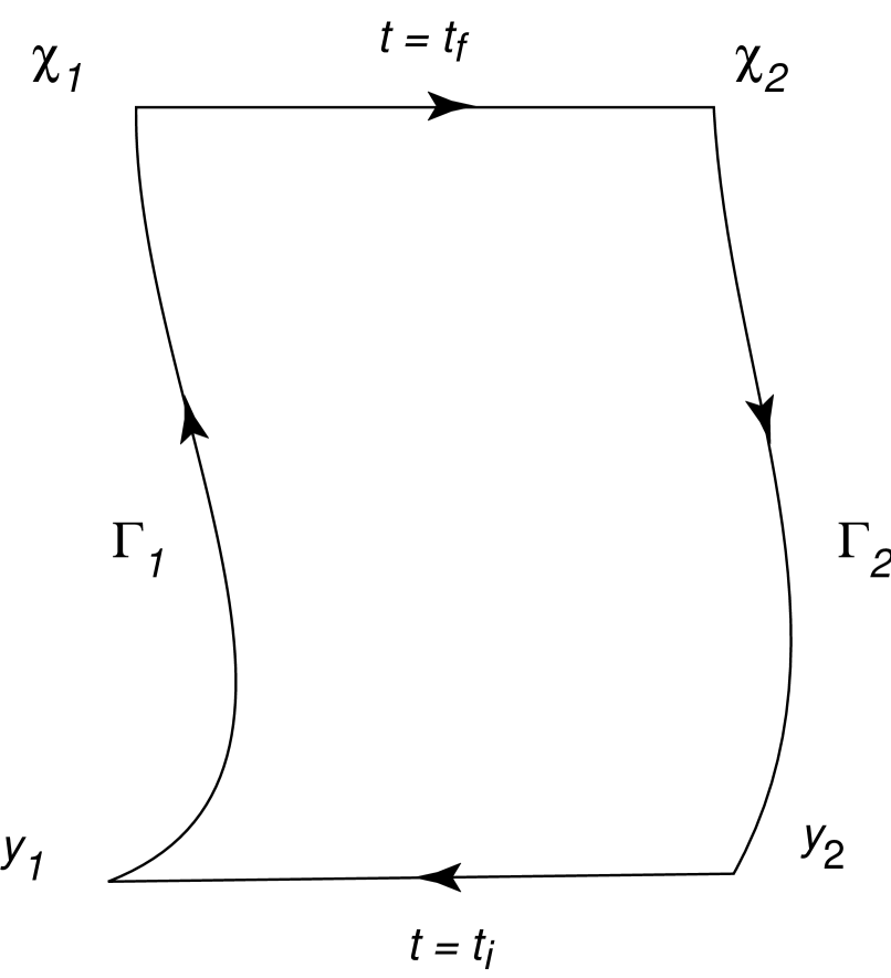
FIG. 1.: Quark-antiquark Wilson loop

REFERENCES

[1] K. G. Wilson, Phys. Rev. D 10, 2445 (1974);
[2] W. Kummer and W. Mödritsch, Z. Phys. C 66, 225
(1995); W. Kummer, W. Mödritsch and A. Vairo,
CERN-TH/96-27, hep-ph/9602276 (1996) (Zeit. Phys. C in press);
[3] W. Buchmüller, Phys. Lett. B 112, 479 (1982);
[4] E. Eichten and F. Feinberg, Phys. Rev. D 23, 2724
(1981); D. Gromes, in Proceedings of the International School of
Physics “Ettore Majorana”, International Science Series
Vol. 37 67 (Plenum, New York, 1989);
M. A. Peskin, in Proceedings of the 11th SLAC Inst.,
SLAC Rep. n.207, 151 ed. by P. Mc. Donough (1993);
[5] D. Gromes, Z. Phys. C 26, 401 (1984);
[6] M. Campostrini, K. Moriarty and C. Rebbi, Phys. Rev. Lett.
57, 44 (1986); K.D. Born, E. Laermann, R. Sommer, T.F. Walsh and
P.M. Zerwas, Phys. Lett. B 329 325 (1994); 332 (1994);
[7] G. S. Bali, K. Schilling and A. Wachter, Nucl. Phys.
B Proc. Suppl. 42, 213 (1995); in Proceedings of “Confinement ’95”
eds. H. Toki et al., p. 82, (World Scientific, Singapore, 1995);
[8] Yu-Qi Chen, Yu-Ping Kuang and R. J. Oakes,
Phys. Rev. D52 264 (1995);
[9] S. N. Gupta, S. F. Randford and W. W. Repko,
Phys. Rev. D 34, 201 (1986);
[10] A. Gara, B. Durand and L. Durand, Phys. Rev.
D 42, 1651 (1990); D 40, 843 (1989);
[11] J. F. Lagae, Phys. Rev. D 45, 305 (1992);
317 (1992); N. Brambilla and G. M. Prosperi, Phys. Rev.
D 48, 2360 (1993); D 46, 1096 (1992);
[12] N. Brambilla, P. Consoli and G. M. Prosperi, Phys. Rev.
D 50, 5878 (1994); N. Brambilla and G. M. Prosperi, in
Proceedings of “Quark Confinement and the Hadron Spectrum”, eds.
N. Brambilla and G. M. Prosperi, p. 113, (World Scientific,
Singapore, 1995);
[13] A. Barchielli, E. Montaldi and G. M. Prosperi,
Nucl. Phys. B 296, 625 (1988);
[14] A. Barchielli, N. Brambilla and G. M. Prosperi,
Nuovo Cimento 103 A, 59 (1990);
[15] Yu. A. Simonov, Nucl. Phys. B 307, 512 (1988);
B 324, 67 (1989);
[16] A. Yu. Dubin, A. B. Kaidalov and Yu. A. Simonov,
Phys. Lett. B 323, 41 (1994);
[17] G. Bali, private communications, see also the
contribution of G. Bali in Proceedings of “Quark Confinement
and the Hadron spectrum II”, eds. N. Brambilla
and G. M. Prosperi (World Scientific, Singapore);
[18] M. Baker, J. Ball and F. Zachariasen, Phys. Rev.
D 51, 1968 (1995); M. Baker, J. S. Ball and F.
Zachariasen, Phys. Rep. 209, 73 (1991); M. Baker, J. S. Ball
and F. Zachariasen, Phys. Lett. B 283, 360 (1992);
[19] M. Baker, J. Ball, N. Brambilla, G. M. Prosperi and
F. Zachariasen, Phys. Rev. D 54, 2829 (1996);
[20] D. La Course and M. G. Olsson, Phys. Rev. D 39, 2751
(1989) and references therein; M. G. Olsson in Proceedings
of “Quark Confinement and the Hadron spectrum”, eds. N. Brambilla
and G. M. Prosperi, p.76 (World Scientific, Singapore, 1995);
M. G. Olsson, and S. Veseli, Phys. Rev D 53, 4006 (1996);
[21] N. Brambilla and G. M. Prosperi, Phys. Rev.
D 47, 2107 (1993); N. Brambilla, G. M. Prosperi and
A. Vairo, Phys. Lett. B 362, 113 (1995);
[22] W. Lucha, F. F. Schöberl and D. Gromes,
Phys. Rep. 200, 127 (1990);
[23] N. Brambilla and G. M. Prosperi, Phys. Lett.
B 236, 69 (1990);
[24] M. G. Olsson, S. Veseli and K. Williams,
Phys. Rev. D 52, 5141 (1995); D 53, 504 (1996);
[25] H. G. Dosch, Phys. Lett. B 190, 177 (1987);
H. G. Dosch and Yu. A. Simonov, Phys. Lett. B 205, 339 (1988);
M. Schiestl and H. G. Dosch, Phys. Lett. B 209, 85 (1988);
[26] Yu. A. Simonov, Yad. Fiz. 54, 192 (1991);
H. G. Dosch, Prog. Part. Nucl. Phys. 33, 121 (1994);
[27] M. Rueter, H. G. Dosch, Z. Phys. C 66, 245 (1995);
[28] Yu. A. Simonov Phys. At. Nucl. 58, 107 (1995);
in Proceedings of “Perturbative and Nonperturbative Aspects
of Quantum Field Theory”, (Schladming, 1996);
[29] I. Ya. Aref’eva, Teor. Mat. Fiz. 43,
111 (1980); N. Bralic, Phys. Rev. D 22, 3090 (1980);
P. M. Fishbane, S. Gasiorowicz and P. Kaus, Phys. Rev.
D 24, 2324 (1981);
[30] Yu. A. Simonov Yad. Fiz. 50, 213 (1989);
[31] N. G. Van Kampen, Phys. Rep. 24 C, 171 (1976);
[32] M. Campostrini, A. Di Giacomo and G. Mussardo,
Z. Phys. C 25, 173 (1984); A. Di Giacomo and H. Panagopoulos
Phys. Lett. B 285, 133 (1992); A. Di Giacomo, E. Meggiolaro
and H. Panagopoulos, (March 1996) hep-lat/9603017;
[33] A. M. Badalian and Yu. A. Simonov,
Spin-dependent potentials and field correlators in QCD
in preparation (1996);
[34] A. M. Badalian and V. P. Yurov, Yad. Fiz. 51, 1368
(1990); Phys. Rev. D 42, 3138 (1990);
[35] M. Baker, J. S. Ball, N. Brambilla and A. Vairo, Nonperturbative evaluation of a field correlator appearing in the
heavy quarkonium system, IFUM 537/FT, hep-ph/9609233 (1996)
(Phys. Lett. B in press);
[36] S. Mandelstam, Phys. Rep. 23 C, 145 (1976);
G. t’Hooft, in ”Proc. Eur. Phys. Soc. 1975”, 1225, ed. by A. Zichichi
(Ed. Comp. Bologna 1976);
[37]P. A. M. Dirac, Phil. Mag. 39, 537 (1920);
[38] M. Baker in Proceedings of the “Workshop
on Quantum Infrared Physics”, Eds. H.M. Fried, B. Muller,
(World Scientific, Singapore, 1995); M. Baker, J. S. Ball and F. Zachariasen,
Int. Jour. Mod. Phys. A 11, 343 (1996);
A. M. Green, C. Michael and P. S. Spencer, HU-TFT-96-36 in Proceedings
of “Quark Confinement and the Hadron spectrum II”, eds. N. Brambilla
and G. M. Prosperi (World Scientific, Singapore);
[39] N. Brambilla, E. Montaldi and G. M. Prosperi,
Phys. Rev. D 54, 3506 (1996);
[40] J. Pantaleone and S. H. Tye, Phys. Rev. D 37,
3337 (1988);
[41]H. G. Dosch, E. Ferreira, A. Krämer, Phys. Rev.
D 50, 1992 (1994);
[42]J. A. M. Vermaseren, Symbolic manipulation with FORM,
(Computer Algebra Nederland, Amsterdam, 1991).