Baryon Magnetic Moments and Proton Spin :
A Model with Collective Quark Rotation

Abstract

We analyse the baryon magnetic moments in a model that relates them to the parton spins $\Delta u$, $\Delta d$, $\Delta s$, and includes a contribution from orbital angular momentum. The specific assumption is the existence of a 3-quark correlation (such as a flux string) that rotates with angular momentum $\langle L_{z}\rangle$ around the proton spin axis. A fit to the baryon magnetic moments, constrained by the measured values of the axial vector coupling constants $a^{(3)}=F+D$, $a^{(8)}=3F-D$, yields $\langle S_{z}\rangle=0.08\pm 0.13$, $\langle L_{z}\rangle=0.39\pm 0.09$, where the error is a theoretical estimate. A second fit, under slightly different assumptions, gives $\langle L_{z}\rangle=0.37\pm 0.09$, with no constraint on $\langle S_{z}\rangle$. The model provides a consistent description of axial vector couplings, magnetic moments and the quark polarization $\langle S_{z}\rangle$ measured in deep inelastic scattering. The fits suggest that a significant part of the angular momentum of the proton may reside in a collective rotation of the constituent quarks.

I Introduction

The question of the angular momentum composition of the proton, first raised in the context of the quark parton model in 1974 [1], has developed into a burning issue, following experiments on polarized deep inelastic scattering, and progress in the theoretical understanding of QCD. Within the quark parton model, the contribution of polarized quarks and antiquarks to the spin of a polarized proton ($J_{z}=1/2$) is [1]

$$\langle S_{z}\rangle = \frac{1}{2}(\Delta u+\Delta d+\Delta s)\equiv\frac{1}{2}\Delta\Sigma$$ (1)

$$\mbox{with}\quad\Delta\Sigma = (3F-D)+\delta_{\mathrm{EJ}}$$ (2)

Here $\Delta q$ is the net polarization of quarks of flavour $q$, $\Delta q=\int dx[\{q_{+}(x)-q_{-}(x)\}+\{\bar{q}_{+}(x)-\bar{q}_{-}(x)\}]$, $F$ and $D$ are the axial vector coupling constants of $\beta$-decay ( $F=0.462\pm 0.01$, $D=0.794\pm 0.01$; Ref. [2] ), and $\delta_{\mathrm{EJ}}$ is the “defect” in the Ellis-Jaffe sum rule [3]

$$\delta_{\mathrm{EJ}}=\int g_{1}^{p}(x)dx-\left(\frac{1}{2}F-\frac{1}{18}D\right)$$ (3)

In QCD, the expression for $\Delta\Sigma$ is modified by perturbative gluon corrections [4] and by a contribution from the gluon anomaly in the singlet axial vector current [5], and reads

$$\Delta\Sigma=(3F-D)+\delta_{\mathrm{EJ}}(Q^{2})+\delta_{\mathrm{anomaly}}$$ (4)

where, to lowest order in $\alpha_{s}/\pi$,

$$\delta_{\mathrm{EJ}}(Q^{2})=\left(1-\frac{\alpha_{s}(Q^{2})}{\pi}\right)^{-1}\int g_{1}^{p}(x,Q^{2})dx-\left(\frac{1}{2}F-\frac{1}{18}D\right)$$ (5)

$$\delta_{\mathrm{anomaly}}=n_{f}\frac{\alpha_{s}}{2\pi}\Delta G$$ (6)

Here $\Delta G$ is the net gluon polarization, $\Delta G=\int dx[G_{+}(x)-G_{-}(x)]$, and $n_{f}=3$ is the number of light quark flavours. A number of authors [6] have analysed the data [7] on the structure functions $g_{1}^{p,n}$, and have reached the conclusion that, barring a large correction from the anomalous term $\delta_{\mathrm{anomaly}}$, $\Delta\Sigma$ lies in the interval

$$\Delta\Sigma\simeq(0.1\ldots 0.3)$$ (7)

Thus the polarization of the quarks and antiquarks accounts for only $10-30\%$ of the spin of the proton, a typical solution for the spin decomposition being $\Delta u=0.83\pm 0.03$, $\Delta d=-0.43\pm 0.03$, $\Delta s=-0.10\pm 0.03$ [8].

II The baryon magnetic moments

In Ref. [1], a tentative attempt was made to relate the nucleon magnetic moments to the spin structure of the proton, encoded in the parameters $\Delta u$, $\Delta d$, $\Delta s$. This idea has recently been generalized to the full baryon octet in two papers [9, 10] that have investigated the following ansatz for the magnetic moments :

$$\mu(p) = \mu_{u}\delta u+\mu_{d}\delta d+\mu_{s}\delta s$$ (8)

$$\mu(n) = \mu_{u}\delta d+\mu_{d}\delta u+\mu_{s}\delta s$$ (9)

$$\mu(\Sigma^{+}) = \mu_{u}\delta u+\mu_{d}\delta s+\mu_{s}\delta d$$ (10)

$$\mu(\Sigma^{-}) = \mu_{u}\delta s+\mu_{d}\delta u+\mu_{s}\delta d$$ (11)

$$\mu(\Xi^{-}) = \mu_{u}\delta s+\mu_{d}\delta d+\mu_{s}\delta u$$ (12)

$$\mu(\Xi^{0}) = \mu_{u}\delta d+\mu_{d}\delta s+\mu_{s}\delta u$$ (13)

$$\mu(\Lambda^{0}) = \frac{1}{6}(\delta u+4\delta d+\delta s)(\mu_{u}+\mu_{d})+\frac{1}{6}(4\delta u-2\delta d+4\delta s)\mu_{s}$$ (14)

The baryon magnetic moments are linear combinations of $\delta u$, $\delta d$, $\delta s$, defined by $\delta q=\int dx[\{q_{+}(x)-q_{-}(x)\}-\{\bar{q}_{+}(x)-\bar{q}_{-}(x)\}]$, which differs from $\Delta q$ in the sign of the antiquark contribution. We consider two hypotheses for the relation between $\delta q$ and $\Delta q$:

• Antiquarks in a polarized baryon reside entirely in a cloud of spin-zero mesons. In this case, antiquarks have no net polarisation, i.e. $\bar{q}_{+}-\bar{q}_{-}=0$, so that $\delta q=\Delta q$. Models of this type have been discussed, for instance, by Cheng and Li [11].

• Antiquarks in a polarized baryon are generated entirely by the pertubative splitting of gluons $g\to q\bar{q}$. In such a case, it is reasonable to expect $\bar{u}_{+}-\bar{u}_{-}\approx\bar{d}_{+}-\bar{d}_{-}\approx\bar{s}_{+}-\bar{s}_{-}\approx s_{+}-s_{-}$. The corresponding relation between $\delta q$ and $\Delta q$ is $\delta u=\Delta u-\Delta s$, $\delta d=\Delta d-\Delta s$, $\delta s=0$ (see, e.g. Ref. [10]).

Below, we give the results of fits to the baryon magnetic moments based on each of the above two hypotheses.

Fit A. Assumption A implies that Eqs.(7) may be rewritten with $\delta q$ replaced by $\Delta q$. Such an approximation was considered by Karl [9], who concluded that the data could be fitted with values of $\Delta u$, $\Delta d$, $\Delta s$ similar to those deduced from polarized deep inelastic scattering, and that the fit was superior to that given by the conventional quark model characterised by $\Delta u=4/3$, $\Delta d=-1/3$, $\Delta s=0$. Our own results for model A are shown in Table 1. As in Ref. [9], each magnetic moment was assigned a theoretical uncertainty of $\pm 0.1\mu_{N}$. This (arbitrary) choice ensures that the various magnetic moments have approximately equal weight and that the fits have a $\chi^{2}$ of about one unit per degree of freedom. The conventional quark model result is given under the appellation “Model 0”. Note that this model necessarily implies a nucleon axial vector coupling $G_{A}\equiv a^{(3)}=F+D=\Delta u-\Delta d=5/3$, in conflict with the measured value 1.26. Notice also that the fit deviates markedly from the expectation $\mu_{u}=-2\mu_{d}$. By contrast, the column labelled “Model AI” gives the result of a fit to Eqs.(7) in which $\Delta u$ and $\Delta d$ are constrained to give the correct value of $G_{A}$, i.e. $G_{A}=1.26$. Additionally, we take $\mu_{u}=-2\mu_{d}$ and $\mu_{s}=3/5\mu_{d}$ (the latter assumption agrees with the fitted value in Ref. [9], and also with the usual constituent quark model estimate $m_{d}/m_{s}=0.6$). It is convenient to rewrite $\Delta u$, $\Delta d$, $\Delta s$ as

$$\Delta u = \frac{2}{3}S_{z}+\frac{1}{2}G_{A}+\frac{1}{6}a^{(8)}$$ (15)

$$\Delta d = \frac{2}{3}S_{z}-\frac{1}{2}G_{A}+\frac{1}{6}a^{(8)}$$ (16)

$$\Delta s = \frac{2}{3}S_{z}-\frac{1}{3}a^{(8)}$$ (17)

so that the magnetic moments in Eq. (7) can be treated as functions of three parameters $\mu_{u}$, $S_{z}=\frac{1}{2}(\Delta u+\Delta d+\Delta s)$ and $a^{(8)}=\Delta u+\Delta d-2\Delta s$. The results of the fit are

$$\mu_{u} = 2.39\pm 0.06$$ (18)

$$S_{z} = 0.14\pm 0.12\qquad\qquad\qquad\mbox{(Model AI)}$$ (19)

$$a^{(8)} = 0.85\pm 0.06$$ (20)

For the central value of $\mu_{u}$, the allowed domain of the parameters $S_{z}$ and $a^{(8)}$ is shown in Fig.1 (ellipse labelled $L_{z}=0$). While the value of $S_{z}$ is in good agreement with the determinations from high energy scattering, there is a clear discrepancy between the value of $a^{(8)}$ obtained from the fit and its experimental value $a^{(8)}=3F-D\approx 0.60$.

Fit B. We now repeat the analysis of the magnetic moments using the ansatz B. Written in terms of $\Delta q$, Eqs.(7) now involve only the combinations $a^{(3)}=\Delta u-\Delta d=G_{A}$ and $a^{(8)}=\Delta u+\Delta d-2\Delta s$, and are independent of the combination $a^{(0)}=\Delta u+\Delta d+\Delta s=2S_{z}$. Accordingly, the fit,

using $G_{A}=1.26$ as input, determines only the two parameters

$$\mu_{u} = 2.40\pm 0.06$$

$$a^{(8)} = 0.82\pm 0.05$$

(Model BI) (21)

no constraint being obtained on $S_{z}$. The allowed domain of these two parameters is shown in Fig.2 by the ellipse labelled $L_{z}=0$. The value of $a^{(8)}$ in Eq.(10) is very similar to the value in Fit A, Eq.(9). In both cases, however, the value of $a^{(8)}$ deviates significantly from the value measured in hyperon decay.

III The rotating proton

In an attempt to resolve the above discrepancy, we have constructed a model containing orbital angular momentum. The total angular momentum of a polarized proton can be resolved as $J_{z}=S_{z}+L_{z}+\Delta G=\frac{1}{2}$. We consider here the effects of an orbital angular momentum $\langle L_{z}\rangle$ associated with the motion of three constituent quarks in the baryon. As pointed out in [1], such orbital motion will produce a correction to the magnetic moments, dependent on the way in which the angular momentum $\langle L_{z}\rangle$ is shared between the constituents. Our central hypothesis is that the quarks in a baryon are held together by a flux string in a “Mercedes-star” configuration. In the plane transverse to the proton spin axis, the quarks will tend to be situated at the corners of an equilateral triangle (Fig.3). Let us imagine that this correlated 3-quark structure rotates collectively around the z-axis, with total orbital angular momentum $\langle L_{z}\rangle$. For a baryon containing constituents $q_{1}$, $q_{2}$, $q_{3}$ with masses $m_{1}$, $m_{2}$, $m_{3}$, the orbital angular momentum carried by the quark $q_{i}$ is $[m_{i}/(m_{1}+m_{2}+m_{3})]\langle L_{z}\rangle$ (we assume rotation about the geometrical centre of the triangle, thereby maintaining SU(3) symmetry in the baryon spatial wave function). With this simple ansatz, we obtain the following corrections to the seven baryon magnetic moments listed in Eq.(7) :

$$\mu(p) = \ldots+\left[2\mu_{u}\left(\frac{1}{3}\right)+\mu_{d}\left(\frac{1}{3}\right)\right]\langle L_{z}\rangle$$ (22)

$$\mu(n) = \ldots+\left[\mu_{u}\left(\frac{1}{3}\right)+2\mu_{d}\left(\frac{1}{3}\right)\right]\langle L_{z}\rangle$$ (23)

$$\mu(\Sigma^{+}) = \ldots+\left[2\mu_{u}\left(\frac{\lambda}{1+2\lambda}\right)+\mu_{s}\left(\frac{1}{1+2\lambda}\right)\right]\langle L_{z}\rangle$$ (24)

$$\mu(\Sigma^{-}) = \ldots+\left[2\mu_{d}\left(\frac{\lambda}{1+2\lambda}\right)+\mu_{s}\left(\frac{1}{1+2\lambda}\right)\right]\langle L_{z}\rangle$$ (25)

$$\mu(\Xi^{-}) = \ldots+\left[\mu_{d}\left(\frac{\lambda}{2+\lambda}\right)+2\mu_{s}\left(\frac{1}{2+\lambda}\right)\right]\langle L_{z}\rangle$$ (26)

$$\mu(\Xi^{0}) = \ldots+\left[\mu_{u}\left(\frac{\lambda}{2+\lambda}\right)+2\mu_{s}\left(\frac{1}{2+\lambda}\right)\right]\langle L_{z}\rangle$$ (27)

$$\mu(\Lambda^{0}) = \ldots+\left[\mu_{u}\left(\frac{\lambda}{1+2\lambda}\right)+\mu_{d}\left(\frac{\lambda}{1+2\lambda}\right)+\mu_{s}\left(\frac{1}{1+2\lambda}\right)\right]\langle L_{z}\rangle$$ (28)

where $\lambda=m_{d}/m_{s}$ is taken to be $0.6$, and the dots “$\ldots$” represent the spin contribution given in Eq.(7).

We have fitted the seven magnetic moments under the same assumptions employed in models A and B (namely, $a^{(3)}=\Delta u-\Delta d=1.26$, $\mu_{u}=-2\mu_{d}$, $\mu_{s}=\frac{3}{5}\mu_{d}$), using $\langle L_{z}\rangle$ as an additional parameter. In a first variation of model A, the parameter $\langle L_{z}\rangle$ was fixed such that $\langle L_{z}\rangle+\langle S_{z}\rangle=\frac{1}{2}$. This represents the extreme hypothesis that the “missing” angular momentum of the proton is precisely accounted for by the orbital angular momentum of the correlated structure depicted in Fig.3. This model then contains the same free parameters as Model AI, namely $\mu_{u}$, $S_{z}$ and $a^{(8)}$. A fit to the magnetic moments (see Table 1) yields

$$\mu_{u} = 2.17\pm 0.09$$ (29)

$$S_{z} = 0.11\pm 0.14\qquad\qquad\qquad\mbox{(Model AII)}$$ (30)

$$a^{(8)} = 0.60\pm 0.10$$ (31)

The quality of the fit is essentially the same as in Model AI, but there is a dramatic improvement in the value of $a^{(8)}$, the result of the fit coinciding with the measured value. This improvement is evident from Fig.1, which shows that with the inclusion of $L_{z}$ there is a convergence of the data on magnetic moments, axial vector couplings and polarized deep inelastic scattering. Within the framework of ansatz A, we can also consider $\langle S_{z}\rangle$ and $\langle L_{z}\rangle$ as independent free parameters, using the experimental value of $a^{(8)}$ as input. A three-parameter fit to the magnetic moments then yields

$$\mu_{u} = 2.17\pm 0.08$$ (32)

$$\langle S_{z}\rangle = 0.08\pm 0.13\qquad\qquad\qquad\mbox{(Model AIII)}$$ (33)

$$\langle L_{z}\rangle = 0.39\pm 0.09$$ (34)

If the effects of orbital angular momentum given by Eqs.(10) are incorporated into model B, we obtain the results indicated in columns BII and BIII in Table 2. A three-parameter fit in terms of $\mu_{u}$, $L_{z}$ and $a^{(8)}$ yields

$$\mu_{u} = 2.10\pm 0.19$$ (35)

$$\langle L_{z}\rangle = 0.54\pm 0.37\qquad\qquad\qquad\mbox{(Model BII)}$$ (36)

$$\langle L_{z}\rangle = 0.49\pm 0.23$$ (37)

On the other hand, if $a^{(8)}=0.6$ is used as input,

we find

$$\mu_{u} = 2.19\pm 0.08$$

$$L_{z} = 0.37\pm 0.09$$

(Model BIII) (38)

The improved convergence of magnetic moment and axial vector coupling data in the presence of orbital angular momentum is evident from Fig.2. Also noteworthy is the similarity in the fitted value of $\langle L_{z}\rangle$ in models A and B, Eqs. (13) and (15). It is certainly intriguing that the value of $\langle L_{z}\rangle$ derived from fits to the static properties of baryons (magnetic moments and axial vector couplings) has the correct sign and approximately the correct magnitude to explain the “spin deficit” of the nucleon revealed by high energy scattering.

IV Conclusion

It would appear from the above that the quark parton model defined by the parton spins $\Delta u$, $\Delta d$, $\Delta s$, can provide a consistent description of axial vector couplings, baryon magnetic moments and the spin structure functions, provided we supplement the spin angular momentum with a collective orbital angular momentum as symbolised in Fig.3. The role of the rotating flux string in achieving this agreement draws renewed attention to flux-string models of the baryon (see e.g. [12] and references therein). Such models have been invoked in the past to explain states in the baryon spectrum (such as the Roper resonance N(1440)) that have not been easy to accomodate in the traditional three-quark picture [13]. The idea that the nucleon may contain $L\neq 0$ components in its wave function (“configuration mixing”) has also been entertained before [14]. The possibility of rotation as a source of hadron spin has been emphasised by Yang [15]. The specific structure introduced in the present paper may be expected, naively, to produce rotational levels with energy $E_{\mathrm{rot}}=J(J+1)/(2I)$, where $I$ is the moment of inertia of the 3-quark correlation. Assuming this structure to consist of three constituent quarks in close contact, each with radius 0.2$-$0.3 fm [16], the excitation energy is 0.5$-$1.0 GeV. It remains to be seen whether the spectrum of baryonic levels will show evidence for states associated with string-like configurations, beyond those that are expected from the shell model with three independently moving quarks. Direct experimental tests for rotating constituents in the nucleon have been proposed in [17], and some tentative evidence from hadronic reactions has been reported [18].

V Acknowlegdement

We wish to record our thanks to Dr. O. Biebel for his help in the error analysis.

Figure Captions

• Fit to baryon magnetic moments in Model A, compared with value of $a^{(8)}$ from hyperon decay, and $S_{z}$ from polarized deep inelastic scattering (bands correspond to $a^{(8)}=0.60\pm 0.05$, $S_{z}=0.10\pm 0.05$). The ellipses labelled $L_{z}=0$ and $L_{z}\neq 0$ correspond to the solutions AI and AII in Table 1.

• Fit to baryon magnetic moments in Model B, compared with value of $a^{(8)}$ from hyperon decay (band corresponds to $a^{(8)}=0.60\pm 0.05$). The ellipses labelled $L_{z}=0$ and $L_{z}\neq 0$ correspond to the solutions BI and BIII in Table 2.

• Flux string connecting three constituent quarks, rotating collectively around proton spin axis

Table Captions

• Fit to baryon magnetic moments in model A. Magnetic moments are in nucleon magnetons and the $\pm 0.1$ is a fictive theoretical error.

• Fit to baryon magnetic moments in model B. Magnetic moments are in nucleon magnetons and the $\pm 0.1$ is a fictive theoretical error.

TABLE 1.
	magn.	Model 0	Model AI	Model AII	Model AIII
	moments	$S_{z}=\frac{1}{2}$, $L_{z}=0$	$S_{z}$ free, $L_{z}=0$	$S_{z}+L_{z}=\frac{1}{2}$	$S_{z}$, $L_{z}$ free
$\mu(p)$	$\begin{array}[]{cc}2.79\pm 0.1\\ \pm 0.00000006\end{array}$	2.67	2.68	2.74	2.74
$\mu(n)$	$\begin{array}[]{cc}-1.91\pm 0.1\\ \pm 0.0000005\end{array}$	$-$1.92	$-$1.84	$-$1.78	$-$1.79
$\mu(\Sigma^{+})$	$\begin{array}[]{cc}2.46\pm 0.1\\ \pm 0.01\end{array}$	2.54	2.58	2.52	2.52
$\mu(\Sigma^{-})$	$\begin{array}[]{cc}-1.16\pm 0.1\\ \pm 0.025\end{array}$	$-$1.14	$-$1.21	$-$1.20	$-$1.20
$\mu(\Xi^{-})$	$\begin{array}[]{cc}-0.65\pm 0.1\\ \pm 0.0025\end{array}$	$-$0.48	$-$0.60	$-$0.60	$-$0.60
$\mu(\Xi^{0})$	$\begin{array}[]{cc}-1.25\pm 0.1\\ \pm 0.014\end{array}$	$-$1.40	$-$1.34	$-$1.38	$-$1.39
$\mu(\Lambda)$	$\begin{array}[]{cc}-0.61\pm 0.1\\ \pm 0.004\end{array}$	$-$0.61	$-$0.60	$-$0.60	$-$0.61
Input		$\begin{array}[]{ccc}\Delta u=\frac{4}{3}\\ \Delta d=-\frac{1}{3}\\ \Delta s=0\end{array}$	$\begin{array}[]{ccc}\mu_{u}=-2\mu_{d}&\\ \mu_{s}=\frac{3}{5}\mu_{d}&\\ G_{A}=1.26\end{array}$	$\begin{array}[]{ccc}\mu_{u}=-2\mu_{d}&\\ \mu_{s}=\frac{3}{5}\mu_{d}&\\ G_{A}=1.26\end{array}$	$\begin{array}[]{cccc}\mu_{u}=-2\mu_{d}\\ \mu_{s}=\frac{3}{5}\mu_{d}&\\ G_{A}=1.26\\ a^{(8)}=0.60\end{array}$
$\chi^{2}/DOF$		$1.82$	$1.12$	$1.105$	$1.095$
$\begin{array}[]{cc}\mbox{fitted}\\ \mbox{param.}\end{array}$		$\begin{array}[]{ccc}\mu_{u}=1.75\pm 0.06\\ \mu_{d}=-1.01\pm 0.06\\ \mu_{s}=-0.61\pm 0.05\end{array}$	$\begin{array}[]{cccc}\mu_{u}=2.17\pm 0.09\\ S_{z}=0.14\pm 0.12\\ a^{(8)}=0.85\pm 0.06\\ \mbox{exp: }0.60\pm 0.02\end{array}$	$\begin{array}[]{cccc}\mu_{u}=2.17\pm 0.09\\ S_{z}=0.11\pm 0.14\\ a^{(8)}=0.60\pm 0.10\\ \mbox{exp: }0.60\pm 0.02\end{array}$	$\begin{array}[]{ccc}\mu_{u}=2.17\pm 0.08\\ S_{z}=0.08\pm 0.13\\ L_{z}=0.39\pm 0.09\end{array}$

TABLE 2.
	magn.	Model 0	Model BI	Model BII	Model BIII
	moments	$S_{z}=\frac{1}{2}$	$S_{z}$ undetermined	$S_{z}$ undetermined	$S_{z}$ undetermined
		$L_{z}=0$	$L_{z}=0$	$L_{z}$ free	$L_{z}$ free
$\mu(p)$	$\begin{array}[]{cc}2.79\pm 0.1\\ \pm 0.00000006\end{array}$	2.67	2.76	2.81	2.80
$\mu(n)$	$\begin{array}[]{cc}-1.91\pm 0.1\\ \pm 0.0000005\end{array}$	$-$1.92	$-$1.78	$-$1.73	$-$1.74
$\mu(\Sigma^{+})$	$\begin{array}[]{cc}2.46\pm 0.1\\ \pm 0.01\end{array}$	2.54	2.65	2.54	2.59
$\mu(\Sigma^{-})$	$\begin{array}[]{cc}-1.16\pm 0.1\\ \pm 0.025\end{array}$	$-$1.14	$-$1.09	$-$1.14	$-$1.13
$\mu(\Xi^{-})$	$\begin{array}[]{cc}-0.65\pm 0.1\\ \pm 0.0025\end{array}$	$-$0.48	$-$0.49	$-$0.54	$-$0.53
$\mu(\Xi^{0})$	$\begin{array}[]{cc}-1.25\pm 0.1\\ \pm 0.014\end{array}$	$-$1.40	$-$1.28	$-$1.36	$-$1.33
$\mu(\Lambda)$	$\begin{array}[]{cc}-0.61\pm 0.1\\ \pm 0.004\end{array}$	$-$0.61	$-$0.52	$-$0.57	$-$0.55
Input		$\begin{array}[]{ccc}\Delta u=\frac{4}{3}\\ \Delta d=-\frac{1}{3}\\ \Delta s=0\end{array}$	$\begin{array}[]{ccc}\mu_{u}=-2\mu_{d}&\\ \mu_{s}=\frac{3}{5}\mu_{d}&\\ G_{A}=1.26\end{array}$	$\begin{array}[]{ccc}\mu_{u}=-2\mu_{d}&\\ \mu_{s}=\frac{3}{5}\mu_{d}&\\ G_{A}=1.26\end{array}$	$\begin{array}[]{cccc}\mu_{u}=-2\mu_{d}\\ \mu_{s}=\frac{3}{5}\mu_{d}&\\ G_{A}=1.26\\ a^{(8)}=0.60\end{array}$
$\chi^{2}/DOF$		$1.82$	$1.99$	$1.72$	$1.43$
$\begin{array}[]{cc}\mbox{fitted}\\ \mbox{param.}\end{array}$		$\begin{array}[]{ccc}\mu_{u}=1.75\pm 0.06\\ \mu_{d}=-1.01\pm 0.06\\ \mu_{s}=-0.61\pm 0.05\end{array}$	$\begin{array}[]{ccc}\mu_{u}=2.40\pm 0.06\\ a^{(8)}=0.82\pm 0.05\\ \mbox{exp: }0.60\pm 0.02\end{array}$	$\begin{array}[]{cccc}\mu_{u}=2.10\pm 0.19\\ L_{z}=0.54\pm 0.37\\ a^{(8)}=0.49\pm 0.23\\ \mbox{exp: }0.60\pm 0.02\end{array}$	$\begin{array}[]{cc}\mu_{u}=2.19\pm 0.08\\ L_{z}=0.37\pm 0.09\end{array}$

FIG. 1.:

FIG. 2.:

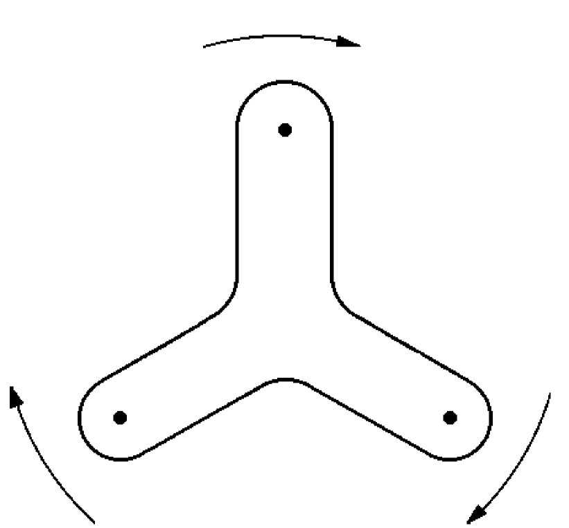
FIG. 3.:

REFERENCES

• [1] L. M. Sehgal, Phys. Rev. D10, 1663 (1974); Erratum ibid. 2016
• [2] X. Song, P. K. Kabir and J. S. McCarthy, hep-ph/9602422
P. G. Ratcliffe, Phys. Lett. B365, 383, (1996)
F. E. Close and R. G. Roberts, Phys. Lett. B316, 165, (1993)
• [3] J. Ellis and R. L. Jaffe. Phys. Rev. D9, 1444, (1974); D10, 1669, (1974)
• [4] J. Kodaira et al., Phys. Rev. D20, 627 (1979)
S. A. Larin, F.V. Tkachev and J. A. M. Vermaseren, Phys. Rev. Lett. 66, 862 (1991)
S. A. Larin and J. A. M. Vermaseren, Phys. Lett. B259, 345 (1991)
S. A. Larin, Phys. Lett. B334, 192 (1994)
• [5] A. V. Efremov and O. V. Teryaev, Dubna report JIN-E2-88-287 (1988)
G. Altarelli and G. Ross, Phys. Lett. B212, 391 (1988)
R. D. Carlitz, J. D. Collins and A. H. Mueller, Phys. Lett. B214, 229 (1988)
• [6] J. Ellis and M. Karliner, hep-ph/9601280
B. L. Ioffe, hep-ph/9511401
G. Altarelli, P. Nason and G. Ridolfi, Phys. Lett. B320, 152 (1994); Erratum, ibid., B325, 538 (1994)
R. Voss, Proc. Workshop on Deep Inelastic Scattering and QCD, Paris (April 1995), Eds. J. F. Laporte and Y. Sirois
M. Anselmino, A. Efremov and E. Leader, Phys. Rep. 261, 1 (1995)
R. L. Jaffe, Physics Today, p.24, Sept. 1995
• [7] SMC collaboration, D. Adams et al., Phys. Lett. B329, 399 (1994); Erratum, ibid., B339, 332 (1994)
SMC collaboration, B. Adeva et al., Phys. Lett. B302, 533 (1993)
E143 collaboration, K. Abe et al., Phys. Rev. Lett. 74, 346 (1995)
E142 collaboration, P. L. Anthony et al., Phys. Rev. Lett. 71, 959 (1995)
EMC collaboration, J. Ashman et al., Phys. Lett. B328, 1 (1989)
• [8] J. Ellis and M. Karliner, Phys. Lett. B342, 397 (1995)
• [9] G. Karl, Phys. Rev. D45, 247 (1992)
• [10] J. Bartelski and R. Rodenberg, Phys. Rev. D41, 2800 (1990)
• [11] T. P. Cheng and Ling-Fong Li, Phys. Lett. B336, 365 (1996). For other approaches to magnetic moments, see
L. Pondrom, Phys. Rev. D53, 5322 (1996)
J. Linde and H. Snellman, Z. Phys. C64, 73 (1994)
G. Dillon and G. Morpurgo, Phys. Rev. D53, 3754 (1996)
L. Brekke and J. L. Rosner, Comments Nucl. Part. Phys. 18, 103 (1988)
• [12] Y. S. Kalashnikova and A. V. Nefediev, Manchester preprint M/C-TH96/1
N. Isgur and J. Paton, Phys. Rev. D31, 2910 (1985)
• [13] R. E. Cutkosky and R. E. Hendrick, Phys. Rev. D16, 786 (1977); ibid. 793
• [14] e.g. S. L. Glashow, Physica 96A, 27 (1979)
• [15] T. T. Chou and C. N. Yang, Nucl. Phys. B107, 1 (1976)
• [16] J. D. Bjorken, SLAC-PUB-95-6949
• [17] Meng Ta-Chung et al., Phys. Rev. D40, 769 (1989)
• [18] C. Boros and Liang Zuo-Tang, Phys. Rev. D53, 2279 (1996)