June 1996
DESY 96-100
hep-ph/9606242
The Coefficient $\eta_{3}$ of the $\mathrm{|\Delta S|\!=\!2}$-Hamiltonian in the Next-To-Leading Order

Abstract

I present the calculation of the QCD short distance coefficient $\eta_{3}$ of the $\mathrm{|\Delta S|\!=\!2}$-hamiltonian in the next-to-leading order (NLO) of renormalization group improved perturbation theory. It involves the two-loop mixing of bilocal structures composed of two $\mathrm{|\Delta S|\!=\!1}$ operators into $\mathrm{|\Delta S|\!=\!2}$ operators. The next-to-leading order corrections enhance $\eta_{3}$ by 27% to

$$\eta_{3}=0.47\raisebox{-2.15277pt}{\shortstack[l]{$\scriptstyle+0.03$\\ $\scriptstyle-0.04$}}$$

thereby affecting the phenomenology of the CP-parameter $\epsilon_{K}$ sizeably. $\eta_{3}$ depends on the physical input parameters $m_{t}$, $m_{c}$ and $\Lambda_{\overline{\mathrm{MS}}}$ only weakly. The quoted error stems from factorization scale dependences, which have reduced compared to the old leading log result. We further discuss some field theoretical aspects of the calculation such as the renormalization group equation for Green’s functions with two operator insertions and the renormalization scheme dependence caused by the presence of evanescent operators. This article is based on work done in collaboration with U. Nierste.

1 Introduction

The effective low-energy hamiltonian inducing the $\mathrm{|\Delta S|\!=\!2}$-transition reads:

$$H^{\mathrm{|\Delta S|\!=\!2}} = \lambda_{c}^{2}H^{c}+\lambda_{t}^{2}H^{t}+2\lambda_{c}\lambda_{t}H^{ct}$$ (1)

$$= \frac{\,G_{F}^{2}}{16\pi^{2}}M_{W}^{2}\biggl{[}\lambda_{c}^{2}\eta_{1}^{\star}S\!\left(x_{c}^{\star}\right)+\lambda_{t}^{2}\eta_{2}^{\star}S\!\left(x_{t}^{\star}\right)$$

$$\hskip 10.00002pt+2\lambda_{c}\lambda_{t}\eta_{3}^{\star}S\!\left(x_{c}^{\star},x_{t}^{\star}\right)\biggr{]}b\!\left(\mu\right)\tilde{Q}_{\mathrm{S2}}\!\left(\mu\right)$$

$$+\mathrm{h.c.}$$

Here $\,G_{F}$ denotes Fermi’s constant, $M_{W}$ is the W boson mass, $\lambda_{j}=V_{jd}V_{js}^{*},j=c,t$ comprises the CKM-factors, and $\tilde{Q}_{\mathrm{S2}}$ is the local dimension-six $\mathrm{|\Delta S|\!=\!2}$ four-quark operator

$$\tilde{Q}_{\mathrm{S2}}=\left[\overline{s}\gamma_{\mu}\left(1-\gamma_{5}\right)d\right]\cdot\left[\overline{s}\gamma_{\mu}\left(1-\gamma_{5}\right)d\right]$$ (2)

The $x_{q}^{\star}={m_{q}^{\star}}^{2}/M_{W}^{2}$, $q=c,t$ encode the running quark masses $m_{q}^{\star}=m_{q}(m_{q})$ in the $\overline{\textrm{MS}}$ scheme. In writing (1) the GIM mechanism $\lambda_{u}+\lambda_{c}+\lambda_{t}=0$ has been used to eliminate $\lambda_{u}$. Further we have set $m_{u}=0$. The Inami-Lim functions $S(x)$, $S(x,y)$ describe the $\mathrm{|\Delta S|\!=\!2}$-transition amplitude in the absence of QCD. They read:

$$S(x_{t}) = x_{t}\left[\frac{1}{4}+\frac{9}{4}\frac{1}{1-x_{t}}-\frac{3}{2}\frac{1}{(1-x_{t})^{2}}\right]$$ (3a)

$$-\frac{3}{2}\left[\frac{x_{t}}{1-x_{t}}\right]^{3}\ln x_{t},$$

$$S(x_{c}) = x_{c}+O(x_{c}^{2}),$$ (3b)

$$S(x_{c},x_{t}) = -x_{c}\ln x_{c}+x_{c}F(x_{t})$$ (3c)

$$+O(x_{c}^{2}\ln x_{c}),$$

with

$$F(x_{t}) = \frac{x_{t}^{2}-8x_{t}+4}{4(1-x_{t})^{2}}\ln x_{t}+\frac{3}{4}\frac{x_{t}}{x_{t}-1}.$$ (4)

In (3b) and (3c) we have only kept terms which are larger than those of order $(m_{s}m_{c})/M_{W}^{2}$ neglected by setting the external momenta to zero.

In (1) the short-distance QCD corrections are comprised in the coefficients $\eta_{1}^{\star}$, $\eta_{2}^{\star}$ and $\eta_{3}^{\star}$ with their explicit dependence on the renormalization scale $\mu$ factored out in the function $b(\mu)$. In absence of QCD corrections $\eta_{i}^{\star}b(\mu)=1$.

Table 1 summarizes the logarithms summed by the forthcoming renormalization group (RG) evolution from $M_{W}$ down to $m_{c}$ in the different orders.

 

Table 1: Logarithms summed by the RG evolution from $M_{W}$ down to $m_{c}$ for the three terms in (1), $n=0,1,2,\ldots$ The last line shows the order in which the dependence on $m_{t}$ enters.

Order		$H^{c}$			$H^{t}$		$H^{ct}$
LO		$(\alpha_{s}\ln\!x_{c})^{n}$			$(\alpha_{s}\ln\!x_{c})^{n}$		$(\alpha_{s}\ln\!x_{c})^{n}$	$\ln\!x_{c}$
NLO	$\alpha_{s}$	$(\alpha_{s}\ln\!x_{c})^{n}$		$\alpha_{s}$	$(\alpha_{s}\ln\!x_{c})^{n}$		$(\alpha_{s}\ln\!x_{c})^{n}$
$m_{t}$		none			in LO		in NLO

 

The first complete determination of the coefficients $\eta_{i}$, $i=1,2,3$ in the leading order (LO) is due to Gilman and Wise [1]. However, the LO expressions have several conceptual drawbacks:

1. The fundamental QCD scale parameter $\Lambda_{\overline{\mathrm{MS}}}$ is not well-defined in the LO.

2. The quark mass dependence of the $\eta_{i}$’s is not correctly reproduced by the LO expressions. Especially the $m_{t}^{\star}$-dependent terms in $\eta_{3}^{\star}\cdot S(x_{c}^{\star},x_{t}^{\star})$ already belong to the NLO.

3. Similarly the question of the definition of the quark masses (i.e. the renormalization scheme and scale) to be used in (1) is a next-to-leading order issue.

4. The LO results for $\eta_{1}$ and $\eta_{3}$ show a large dependence on the factorization scales, at which one integrates out heavy particles. In the NLO these uncertainties are reduced considerably.

5. One must go to the NLO to judge whether perturbation theory works, i.e. whether the radiative corrections are small. After all the corrections can be sizeable.

To overcome the limitations listed above one has to go to the next-to-leading order (NLO). This programme has been started with the calculation of $\eta_{2}^{\star}$ by Buras, Jamin and Weisz [2]. Then Nierste and I have derived the NLO expressions for $\eta_{1}^{\star}$ [3] and $\eta_{3}^{\star}$ [4]. This article will essentially deal with the term $H^{ct}$ of (1) and is based on [4].

2 The NLO calculation of $\eta_{3}$ above the charm threshold

Here we will shortly describe how the large logarithm $\ln x_{c}$ present in (3c) is summed to all orders in perturbation theory. This is done in two steps: First one sets up an effective lagrangian ${\mathcal{L}}_{\mathrm{eff}}^{\mathrm{|\Delta S|\!=\!2}}$ in which the W boson and the top quark are removed as dynamic degrees of freedom. In ${\mathcal{L}}_{\mathrm{eff}}^{\mathrm{|\Delta S|\!=\!2}}$ the $\mathrm{|\Delta S|\!=\!1}$ and $\mathrm{|\Delta S|\!=\!2}$ transitions are described by local four-quark operators, which are multiplied by Wilson coefficients. The general structure of ${\mathcal{L}}_{\mathrm{eff}}^{\mathrm{|\Delta S|\!=\!2}}$ reads:

$${\mathcal{L}}_{\mathrm{eff}}^{\mathrm{|\Delta S|\!=\!2}} = -\frac{\,G_{F}}{\sqrt{2}}V_{\mathrm{CKM}}\sum_{k}C_{k}Q_{k}$$ (5)

$$-\frac{\,G_{F}^{2}}{2}V_{\mathrm{CKM}}\sum_{l}\widetilde{C}_{l}\widetilde{Q}_{l}.$$

Here the $V_{\mathrm{CKM}}$ denote products of CKM elements. The $Q_{k}$, $\widetilde{Q}_{l}$ represent local $\mathrm{|\Delta S|\!=\!1}$ and $\mathrm{|\Delta S|\!=\!2}$ operators and the $C_{k}$, $\widetilde{C}_{l}$ are the corresponding Wilson coefficient functions. The $\mathrm{|\Delta S|\!=\!1}$ part of (5) contributes to $\mathrm{|\Delta S|\!=\!2}$ transitions via diagrams of the type displayed in Fig. 1.

 

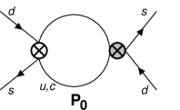
Figure 1: The diagrams $\mathsf{D_{0}}$ and $\mathsf{P_{0}}$ in the effective five- and four-quark theory. The light crosses denote insertions of local $\mathrm{|\Delta S|\!=\!1}$ current-current operators, the grey ones insertion of local $\mathrm{|\Delta S|\!=\!1}$ four-quark penguin operators.

 

The Wilson coefficients are fixed at a factorization scale $\mu_{tW}=O(M_{W},m_{t})$ by the requirement that the $\mathrm{|\Delta S|\!=\!1}$ and $\mathrm{|\Delta S|\!=\!2}$ Green’s functions derived from (5) are equal to the same quantities calculated with the full SM lagrangian. The effect of this procedure is that the $\ln x_{c}$ present in (3c) is split as $\ln(\mu_{tW}/M_{W})+\ln(m_{c}/\mu_{tW})$. Here the former term resides in the Wilson coefficients while the latter is contained in the matrix elements of the local operators. The choice $\mu_{tW}=O(M_{W},m_{t})$ ensures that the Wilson coefficients do not contain large logarithms and therefore can be reliably calculated in ordinary perturbation theory.

The second step is the RG evolution of the Wilson coefficients from the scale $\mu_{tW}$ down to $\mu_{c}=O(m_{c})$ which sums $\ln(\mu_{c}/\mu_{tW})$.

2.1 The Operator Basis

Let us now construct ${\mathcal{L}}_{\mathrm{eff}}^{\mathrm{|\Delta S|\!=\!2}}$ in (5) as far it is needed for the calculation of $\eta_{3}$. Since the presence of $\mathrm{|\Delta S|\!=\!2}$ terms in (5) does not affect the $\mathrm{|\Delta S|\!=\!1}$ part of ${\mathcal{L}}_{\mathrm{eff}}^{\mathrm{|\Delta S|\!=\!2}}$, we can simply take the latter from [5, 6, 7]. They consist of the following set of operators:

$$Q_{1}^{kl} = \left(\bar{s}\gamma_{\mu}Lk\right)\cdot\left(\bar{l}\gamma^{\mu}Ld\right)\cdot\widetilde{\leavevmode\hbox{\small 1\kern-3.8pt\normalsize 1}},$$ (6a)

$$Q_{2}^{kl} = \left(\bar{s}\gamma_{\mu}Lk\right)\cdot\left(\bar{l}\gamma^{\mu}Ld\right)\cdot\leavevmode\hbox{\small 1\kern-3.8pt\normalsize 1},$$ (6b)

$$Q_{3} = \left(\overline{s}\gamma_{\mu}Ld\right)\cdot\sum_{q=d,u,s,\ldots}\left(\overline{q}\gamma^{\mu}Lq\right)\cdot\leavevmode\hbox{\small 1\kern-3.8pt\normalsize 1},$$ (6c)

$$Q_{4} = \left(\overline{s}\gamma_{\mu}Ld\right)\cdot\sum_{q=d,u,s,\ldots}\left(\overline{q}\gamma^{\mu}Lq\right)\cdot\widetilde{\leavevmode\hbox{\small 1\kern-3.8pt\normalsize 1}},$$ (6d)

$$Q_{5} = \left(\overline{s}\gamma_{\mu}Ld\right)\cdot\sum_{q=d,u,s,\ldots}\left(\overline{q}\gamma^{\mu}Rq\right)\cdot\leavevmode\hbox{\small 1\kern-3.8pt\normalsize 1},$$ (6e)

$$Q_{6} = \left(\overline{s}\gamma_{\mu}Ld\right)\cdot\sum_{q=d,u,s,\ldots}\left(\overline{q}\gamma^{\mu}Rq\right)\cdot\widetilde{\leavevmode\hbox{\small 1\kern-3.8pt\normalsize 1}}.$$ (6f)

Here the $Q_{i}^{kl}$, $i\!=\!1,2$, $k,l\!=\!u,c$ represent the $\mathrm{|\Delta S|\!=\!1}$ current-current operators, the $Q_{i}$, $i\!=\!3,\ldots,6$ the QCD-penguin operators. The sum in (6c)–(6f) runs over all active flavours. Further $L,R=(1\mp\gamma_{5})$ and 11, $\widetilde{\leavevmode\hbox{\small 1\kern-3.8pt\normalsize 1}}$ denote color singlet and anti-singlet, i.e. $Q_{1}^{kl}=\left(\overline{s}_{i}\gamma_{\mu}Lk_{j}\right)\cdot\left(\overline{l}_{j}{\gamma^{\mu}}Ld_{i}\right)$ with $i,j$ being color indices.

Further we need the $\mathrm{|\Delta S|\!=\!2}$ operators present in (5). Consider first the diagram $\mathsf{D_{0}}$ of Fig. 1 with two internal charm quarks and zero external momenta. The only physical dimension-eight $\mathrm{|\Delta S|\!=\!2}$ operator required to absorb its divergence reads

$$\widetilde{Q}_{7} = \frac{m_{c}^{2}}{g^{2}\mu^{2\varepsilon}}\tilde{Q}_{\mathrm{S2}}=\frac{m_{c}^{2}}{g^{2}\mu^{2\varepsilon}}\cdot\overline{s}\gamma_{\mu}Ld\cdot\overline{s}\gamma^{\mu}Ld,$$ (7)

which follows from power counting and the absence of any non-zero mass parameter apart from $m_{c}$. The inverse powers of $g$ are introduced for later convenience as in [1]. One may arbitrarily shift such factors from the Wilson coefficient into the definition of the operator. The factor $\mu^{-2\varepsilon}$ stems from $g_{\mathrm{bare}}=Z_{g}g\mu^{\varepsilon}$ and the fact that

$$\widetilde{Q}_{7}^{\mathrm{bare}} = \frac{m_{c,\,\mathrm{bare}}^{2}}{g_{\mathrm{bare}}^{2}}\left[\overline{s}\gamma_{\mu}Ld\cdot\overline{s}\gamma^{\mu}Ld\right]^{\mathrm{bare}}.$$ (8)

must be independent of $\mu$. Any other dimension-eight $\mathrm{|\Delta S|\!=\!2}$ operator contains one or two powers of $m_{c}$ less than $\widetilde{Q}_{7}$ and derivatives and/or gluon fields instead. Their on-shell matrix elements are suppressed by powers of $m_{s}/m_{c}$ with respect to those of $\widetilde{Q}_{7}$, so that they do not contribute to the coefficient of the leading dimension-six operator below the charm threshold (cf. (1)). Likewise they cannot mix with $\widetilde{Q}_{7}$ under renormalization.

Therefore our operator basis consists of $Q_{1,2}^{kl}$, $Q_{3,\ldots,6}$ and $\widetilde{Q}_{7}$and ${\mathcal{L}}_{\mathrm{eff}}^{\mathrm{|\Delta S|\!=\!2}}$ is found as:

$${\mathcal{L}}_{\mathrm{eff}}^{\mathrm{|\Delta S|\!=\!2}} \!\!\!\!=\!\!\!\! -\frac{\,G_{F}}{\sqrt{2}}\sum_{i=1}^{6}C_{i}\biggl{[}\sum_{j=1}^{2}Z^{-1}_{ij}\sum_{k,l=u,c}V_{ks}^{\ast}V_{ld}Q_{j}^{kl,\mathrm{bare}}$$ (12)

$$\hskip 60.00009pt-\lambda_{t}\sum_{j=3}^{6}Z^{-1}_{ij}Q_{j}^{\mathrm{bare}}\biggr{]}$$

$$-\frac{\,G_{F}^{2}}{2}\lambda_{c}\lambda_{t}\biggl{[}\sum_{k=1}^{2}\sum_{l=1}^{6}C_{k}C_{l}\widetilde{Z}_{kl,7}^{-1}$$

$$\hskip 60.00009pt+\widetilde{C}_{7}\widetilde{Z}_{77}^{-1}\biggr{]}\widetilde{Q}_{7}^{\mathrm{bare}}$$

$$+\parbox[t]{140.00021pt}{counterterms proportional to unphysical operators.}$$

2.2 The Effective Lagrangian ${\mathcal{L}}_{\mathrm{eff}}^{\mathrm{|\Delta S|\!=\!2}}$ at the Scale $\mu_{tW}$

Besides the operators we need to know their corresponding Wilson coefficient functions at the initial scale $\mu_{tW}$. The ones for the $\mathrm{|\Delta S|\!=\!1}$ case, $C_{i}$, $i\!=\!1,\ldots,6$ can be taken from [5, 6, 7]. It is important to note that only $C_{2}$ starts at $O(\alpha_{s}^{0})$, the others at $O(\alpha_{s}^{1})$. This means that the NLO matching can be done solely with the diagram $\mathsf{D_{0}}$ of Fig. 1 with two insertions of $Q_{2}$. One easily finds

$$\widetilde{C}_{7}(\mu_{tW})=\left\{\begin{array}[]{@{}ll}0&\mbox{in LO}\\ \displaystyle\frac{\alpha_{s}(\mu_{tW})}{4\pi}\bigl{(}-8\ln\frac{\mu_{tW}}{M_{W}}&\\ \hskip 5.0pt+4F\left(x_{t}\left(\mu_{tW}\right)\bigr{)}+2\right)&\mbox{in NLO}\end{array}\right.,$$ (13)

where $F(x_{t})$ is the top dependent part of $S(x_{c},x_{t})$ defined in (4). The factor $\alpha_{s}$ originates from the special definition of $\widetilde{Q}_{7}$ in (7). Note how the large logarithm $\ln x_{c}$ in (3c) is split between the Wilson coefficient $\widetilde{C}_{7}$ and the matrix element. The NLO result in (13) is specific to the NDR scheme with (11).

2.3 Evolving down ${\mathcal{L}}_{\mathrm{eff}}^{\mathrm{|\Delta S|\!=\!2}}$ from $\mu_{tW}$ to $\mu_{c}$

Next we have to evolve down the Wilson coefficients present in ${\mathcal{L}}_{\mathrm{eff}}^{\mathrm{|\Delta S|\!=\!2}}$ (12) from $\mu_{tW}$ to $\mu_{c}$. For the $\mathrm{|\Delta S|\!=\!1}$ functions $C_{i}$, $i\!=\!1,\ldots,6$ this is achieved by standard methods [6]. To calculate the running of the $\mathrm{|\Delta S|\!=\!2}$ coefficient $\widetilde{C}_{7}$ we need to derive and solve the corresponding RG equation. From $\mu\frac{d}{d\mu}{\mathcal{L}}_{\mathrm{eff}}^{\mathrm{|\Delta S|\!=\!2}}=0$ in (12) one finds

$$\mu\frac{d}{d\mu}\widetilde{C}_{7}\left(\mu\right) = \widetilde{C}_{7}\left(\mu\right)\widetilde{\gamma}_{77}$$ (14)

$$+\sum_{k=1}^{2}\sum_{k^{\prime}=1}^{6}C_{k}\left(\mu\right)C_{k^{\prime}}\left(\mu\right)\widetilde{\gamma}_{kk^{\prime},7}$$

with the anomalous dimension tensor

$$\widetilde{\gamma}_{kn,7} = \frac{\alpha_{s}}{4\pi}\widetilde{\gamma}_{kn,7}^{\left(0\right)}+\left(\frac{\alpha_{s}}{4\pi}\right)^{2}\widetilde{\gamma}_{kn,7}^{\left(1\right)}+\ldots$$ (15)

$$= -\sum_{k^{\prime}=1}^{2}\sum_{n^{\prime}=1}^{6}\left[\gamma_{kk^{\prime}}\delta_{nn^{\prime}}+\delta_{kk^{\prime}}\gamma_{nn^{\prime}}\right]\widetilde{Z}_{k^{\prime}n^{\prime},7}^{-1}\widetilde{Z}_{77}$$

$$-\left[\mu\frac{d}{d\mu}\widetilde{Z}_{kn,7}^{-1}\right]\widetilde{Z}_{77}.$$

It is possible to solve the inhomogeneous equation (14) directly but this turns out to be inconvenient for practical purposes. Instead we may combine the evolution equations of the $\mathrm{|\Delta S|\!=\!1}$ and $\mathrm{|\Delta S|\!=\!2}$ Wilson coefficients into a single matrix equation. This is made possible because the GIM mechanism ensures that at least one of the two $\mathrm{|\Delta S|\!=\!1}$ operator insertions in diagrams like the ones displayed in Fig. 1 is of the current-current type. The current-current part of the $\mathrm{|\Delta S|\!=\!1}$ mixing matrix, i.e. the entries related to $Q_{1}$, $Q_{2}$, can be diagonalized exactly using the basis

$$Q_{\pm}^{kl}=\frac{1}{2}\left(Q_{2}^{kl}\pm Q_{1}^{kl}\right).$$ (16)

Then (14) together with the RG equation of the $\mathrm{|\Delta S|\!=\!1}$ Wilson coefficients splits into two independent inhomogeneous RG equations

$$\mu\frac{d}{d\mu}\widetilde{C}_{7}^{\pm}\left(\mu\right)=\widetilde{\gamma}_{77}\widetilde{C}_{7}^{\pm}\left(\mu\right)+\widetilde{\gamma}_{\pm k,7}C_{\pm}\left(\mu\right)C_{k}\left(\mu\right).$$ (17)

Here the decomposition of $\widetilde{C}_{7}(\mu_{tW})$ into $\widetilde{C}_{7}^{\pm}(\mu_{tW})$ is completely arbitrary provided one satisfies

$$\widetilde{C}_{7}\left(\mu_{tW}\right)=\widetilde{C}_{7}^{+}\left(\mu_{tW}\right)+\widetilde{C}_{7}^{-}\left(\mu_{tW}\right).$$ (18)

This decomposition is then automatically preserved at any renormalization scale.

Each of the two equations in (17) may be written as a 7$\times$7 matrix equation, which may be solved by standard methods. We can even do better and collapse the two resulting 7$\times$7 matrix equations into one 8$\times$8 matrix equation:

$$\mu\frac{d}{d\mu}\vec{D}=\widehat{\gamma}^{T}\cdot\vec{D}$$ (19)

with

$$\widehat{\gamma}^{T} = \left(\begin{array}[]{ccc}\gamma^{T}&0&0\\ \widetilde{\gamma}_{+,7}^{T}&\widetilde{\gamma}_{77}-\gamma_{+}&0\\ \widetilde{\gamma}_{-,7}^{T}&0&\widetilde{\gamma}_{77}-\gamma_{-}\end{array}\right)$$ (20d)

$$\widetilde{\gamma}_{\pm,7}^{T} = \left(\widetilde{\gamma}_{\pm 1\!,7},\widetilde{\gamma}_{\pm 2\!,7},\widetilde{\gamma}_{\pm 3\!,7},\widetilde{\gamma}_{\pm 4\!,7},\widetilde{\gamma}_{\pm 5\!,7},\widetilde{\gamma}_{\pm 6\!,7}\right)$$ (20e)

$$\vec{D}\left(\mu\right) = \left(\begin{array}[]{c}\vec{C}\left(\mu\right)\\ \widetilde{C}_{7}^{+}\left(\mu\right)/C_{+}\left(\mu\right)\\ \widetilde{C}_{7}^{-}\left(\mu\right)/C_{-}\left(\mu\right)\end{array}\right).$$ (20i)

We now need to know the elements of the anomalous dimension tensor $\widetilde{\gamma}_{\pm i,7}$, $i=1,\ldots,6$. They are obtained from the renormalization constants using the definition in (15) and expanding the quantities in there in powers of $\alpha_{s}$ and $1/\varepsilon$. Here it is important to include the finite renormalization terms needed for the correct treatment of the evanescent operators (9). To calculate the LO term $\widetilde{\gamma}_{\pm i,7}^{(0)}$ one needs to know the $1/\varepsilon$ parts of the one-loop diagrams displayed in Fig. 1, the NLO part $\widetilde{\gamma}_{\pm i,7}^{(1)}$ requires the evaluation of a set of two-loop graphs. We find:

$$\widetilde{\gamma}_{+,7}^{(0)}=\left(\begin{array}[]{r}-16\\ -8\\ -32\\ -16\\ 32\\ 16\end{array}\right), \widetilde{\gamma}_{-,7}^{(0)}=\left(\begin{array}[]{r}8\\ 0\\ 16\\ 0\\ -16\\ 0\end{array}\right),$$ (21m)

$$\widetilde{\gamma}_{+,7}^{(1)}=\left(\begin{array}[]{r}-212\\ -28\\ -456\\ -88\\ \frac{1064}{3}\\ \frac{832}{3}\end{array}\right), \widetilde{\gamma}_{-,7}^{(1)}=\left(\begin{array}[]{r}276\\ -92\\ 520\\ -216\\ -\frac{1288}{3}\\ 0\end{array}\right).$$ (21z)

As usual the NLO anomalous dimension tensor depends on the renormalization scheme. The result (21z) corresponds to the NDR scheme with the definition of the evanescent operators corresponding to (11).

3 The NLO calculation of $\eta_{3}$ below the charm threshold

3.1 The Effective Lagrangian ${\mathcal{L}}_{\mathrm{eff}}^{\mathrm{|\Delta S|\!=\!2}}$ at the Scale $\mu_{c}=O(m_{c})$

After integrating out the charm quark all dependence on $m_{c}$ belongs to the Wilson coefficients. This implies that the term involving $\widetilde{Q}_{7}$ in (12) has to disappear from the effective lagrangian, because $\widetilde{Q}_{7}$ contains $m_{c}$ in its definition (7). Further the $\mathrm{|\Delta S|\!=\!1}$ operators are neglected in the new effective lagrangian, because the matrix elements of double insertions of these operators are at most proportional to $m_{s}^{2}$ rather than $m_{c}^{2}$. We have already neglected such terms in all preceding steps.

Therefore the new effective lagrangian to describe the physics below $\mu_{c}$ reads:

$${\mathcal{L}}_{\mathrm{eff}}^{\mathrm{|\Delta S|=2}} = -\frac{\,G_{F}^{2}}{16\pi^{2}}\biggl{[}\lambda_{c}^{2}\widetilde{C}_{\mathrm{S2}}^{(c)}\left(\mu\right)+\lambda_{t}^{2}\widetilde{C}_{\mathrm{S2}}^{(t)}\left(\mu\right)$$ (23)

$$+\lambda_{c}\lambda_{t}\widetilde{C}_{\mathrm{S2}}^{(ct)}\left(\mu\right)\biggr{]}\widetilde{Z}_{\mathrm{S2}}^{-1}\left(\mu\right)\tilde{Q}_{\mathrm{S2}}^{\mathrm{bare}}.$$

This lagrangian already resembles $-H^{\mathrm{|\Delta S|\!=\!2}}$ introduced in (1). For the matching we have to set the Green’s function derived from (12) and the one derived from (23) equal at the scale $\mu=\mu_{c}$.

Let us start with the matching of $\widetilde{C}_{7}$ in the LO: since the definition of $\widetilde{Q}_{7}$ (7) contains the factor $\alpha_{s}$ with respect to $\tilde{Q}_{\mathrm{S2}}$ we develop an explicit inverse power of $\alpha_{s}$ for the Wilson coefficient:

$$\widetilde{C}_{\mathrm{S2}}^{(ct)}\left(\mu_{c}\right) = \frac{m_{c}^{2}\left(\mu_{c}\right)}{2}\frac{4\pi}{\alpha_{s}\left(\mu_{c}\right)}\widetilde{C}_{7}\left(\mu_{c}\right)\mbox{in LO}.$$ (24)

Diagrams containing double insertions are of order $\alpha_{s}^{0}$ and therefore start contributing to $\widetilde{C}_{\mathrm{S2}}^{(ct)}$ in the NLO. The NLO version of $\widetilde{C}_{\mathrm{S2}}^{(ct)}$ can be written

$$\widetilde{C}_{\mathrm{S2}}^{(ct)}\left(\mu_{c}\right) = m_{c}^{2}\left(\mu_{c}\right)\biggl{[}\frac{1}{2}\frac{4\pi}{\alpha_{s}\left(\mu_{c}\right)}\widetilde{C}_{7}\left(\mu_{c}\right)$$ (25)

$$+\sum_{i=+,-}\sum_{j=1}^{6}r_{ij,S2}\left(\mu_{c}\right)C_{i}\left(\mu_{c}\right)C_{j}\left(\mu_{c}\right)\biggr{]}.$$

The coefficients $r_{ij,S2}\left(\mu_{c}\right)$ in (25) are given by the finite parts of the diagrams in Fig. 1. We find:

$$r_{ij,S2}\left(\mu_{c}\right) = \left\{\begin{array}[]{l@{\hspace{0.3em}\mbox{for }j=\hspace{-0.2em}}l}\displaystyle\left[-4\ln\frac{m_{c}(\mu_{c})}{\mu_{c}}-1\right]\tau_{ij}\hfil\hskip 3.00003pt&1,2,\\[12.05553pt] \displaystyle\left[-8\ln\frac{m_{c}(\mu_{c})}{\mu_{c}}-4\right]\tau_{ij}\hfil\hskip 3.00003pt&3,4,\\[12.05553pt] \displaystyle\left[8\ln\frac{m_{c}(\mu_{c})}{\mu_{c}}+4\right]\tau_{ij}\hfil\hskip 3.00003pt&5,6,\end{array}\right.$$ (29)

where the $\tau_{ij}$’s denote the colour factors

$$\begin{array}[]{l}\displaystyle\tau_{\pm 1}=\tau_{\pm 3}=\tau_{\pm 5}=\frac{1\pm N}{2},\\ \displaystyle\tau_{+2}=\tau_{+4}=\tau_{+6}=1,\\ \displaystyle\tau_{-2}=\tau_{-4}=\tau_{-6}=0.\end{array}$$ (33)

Note that $r_{ij,S2}$ for $j=1,2$ depends on the definition of the evanescent operator $E_{1}[\widetilde{Q}_{7}]$. As usual (29) only holds in the NDR scheme.

3.2 Evolving ${\mathcal{L}}_{\mathrm{eff}}^{\mathrm{|\Delta S|\!=\!2}}$ below $\mu_{c}$

The RG running in the effective three quark theory is particularly simple because there is only one operator left: $\tilde{Q}_{\mathrm{S2}}$. The running of the corresponding Wilson coefficient function $\widetilde{C}_{\mathrm{S2}}^{(ct)}$ can be taken from [5, 2].

$\eta_{3}$ can then be determined from the identification

$${\mathcal{L}}_{\mathrm{eff}}^{\mathrm{|\Delta S|\!=\!2}}=-H^{\mathrm{|\Delta S|\!=\!2}}$$ (34)

with ${\mathcal{L}}_{\mathrm{eff}}^{\mathrm{|\Delta S|\!=\!2}}$ from (23) and $H^{\mathrm{|\Delta S|\!=\!2}}$ from (1). The result of this can be found in [4, section 5].

4 Numerical Results

Let us now discuss the numerical implications of the calculation presented in the preceding sections. We will present the dependence of $\eta_{3}^{\star}$ on its various physical parameters and on the renormalization scales at which particles are integrated out.

$\eta_{3}^{\star}$ depends on the scales $\mu_{tW}$, $\mu_{b}$ and $\mu_{c}$. Further it is a function of the masses $m_{t}$, $m_{c}$ and of the QCD scale parameter $\Lambda_{\mathrm{QCD}}$. To establish a starting point let us pick a basic set of input parameters

$$\begin{array}[]{*{2}{l}}\begin{array}[]{@{}l}m_{c}(m_{c})=\mu_{c}\\ \hskip 10.00002pt=1.3\,\mathrm{GeV},\end{array}&\begin{array}[]{@{}l}\Lambda_{\overline{\mathrm{MS}}}=0.31\,\mathrm{GeV},\\ \Lambda_{\mathrm{QCD}}^{\mathrm{LO}}=0.15\,\mathrm{GeV},\end{array}\\ \mu_{b}=4.8\,\mathrm{GeV},&M_{W}=80\,\mathrm{GeV},\\ \mu_{tW}=130\,\mathrm{GeV},&m_{t}(m_{t})=167\,\mathrm{GeV}.\end{array}$$ (42)

In the following $\Lambda_{\mathrm{QCD}}$ is always understood to be defined with respect to four active flavours, the corresponding quantities in effective three- and five flavour-theories are obtained by imposing continuity on the coupling $\alpha_{s}$ at $\mu_{c}$ and $\mu_{b}$.

The value for $\eta_{3}^{\star}$ corresponding to the set (42) reads:

$${\eta_{3}^{\star}}^{\mathrm{LO}}=0.365,\hskip 20.00003pt{\eta_{3}^{\star}}^{\mathrm{NLO}}=0.467.$$ (43)

Hence the NLO calculation has enhanced $\eta_{3}^{\star}$ by 27%. From the difference of 0.102 between the two values in (43) 0.022 originates from the change from the LO to the NLO running $\alpha_{s}$. The smallness of this contribution is caused by the adjustment of $\Lambda_{\mathrm{QCD}}^{\mathrm{LO}}$ to fit the NLO running coupling. The explicit $O(\alpha_{s})$ corrections from the NLO mixing and matching contribute 0.080.

Let us further quantify the influence of the penguin operators $Q_{3,\ldots,6}$: If one neglects them completely, one obtains ${\eta_{3}^{\star}}^{\mathrm{NLO,np}}=0.472$ with the set in (42), i.e. their contribution is of the order of 1%.

4.1 Scale Dependence of $\eta_{3}^{\star}$

Ideally $\eta_{3}^{\star}$ should not depend on the factorization scales $\mu_{tW}$, $\mu_{b}$, $\mu_{tW}$. Yet due to the truncation of the perturbation series such a dependence shows up. It may serve as an estimate of the theoretical error of the calculation.

It turns out that the dependence of $\eta_{3}^{\star}$ on $\mu_{b}$ is extremely mild. This is due to the fact that no diagrams containing internal bottom quarks contribute to the $\mathrm{|\Delta S|\!=\!2}$ process in order $\alpha_{s}$. The only places where $\mu_{b}$ enters are a) the running of $\alpha_{s}$, b) the NLO matching matrices and anomalous dimensions of the $\mathrm{|\Delta S|\!=\!1}$ penguin operators. Numerically one finds that $\eta_{3}^{\star}$ is shifted by 0.1–0.2% if one choses the extreme values of $\mu_{b}\equiv\mu_{c}=O(m_{c})$ or $\mu_{b}\equiv\mu_{tW}=O(m_{W},m_{t})$.

Now let us turn to the more important cases, $\mu_{tW}$ and $\mu_{c}$. First consider the variation of $\eta_{3}^{\star}$ with respect to $\mu_{tW}$, which is displayed in Fig. 2.

 

Figure 2: The variation of $\eta_{3}^{\star}$ in LO and NLO with respect to the scale $\mu_{tW}$, at which the initial condition is defined. The other input parameters are given in (42).

 

Since at $\mu_{tW}$ the top quark and the W-boson are integrated out simultaneously, it is natural to choose the interval $M_{W}\leq\mu_{tW}\leq m_{t}$ for the analysis. In the LO result for $\eta_{3}^{\star}$ we find a sizeable scale dependence of 12%. It is almost totally removed in the NLO, where we obtain a variation of less than 3% in this interval. This shows that it is very accurate to integrate out the two heavy particles simultaneously. The strong improvement in the NLO is due to the smallness of $\ln x_{t}$.

The situation is not so nice in the case of the variation of $\mu_{c}$, which is displayed in Fig. 3.

 

Figure 3: The variation of $\eta_{3}^{\star}$ in LO and NLO with respect to the scale $\mu_{c}$. The range for the latter is taken unphysically large to visualize the breakdown of perturbation theory. The other input parameters are given in (42).

 

We have intentionally extended the range for $\mu_{c}$ to the unphysical low value of $0.7\,\mathrm{GeV}$ to visualize the breakdown of perturbation theory. Varying $\mu_{c}$ within the interval $1.1\,\mathrm{GeV}\leq\mu_{c}\leq 1.6\,\mathrm{GeV}$ yields

$$0.33\leq{\eta_{3}^{\star}}^{\mathrm{LO}}\leq 0.40,\hskip 10.00002pt0.43\leq{\eta_{3}^{\star}}^{\mathrm{NLO}}\leq 0.50.$$ (44)

This corresponds to a reduction of the scale dependence from 20% to 14%. One reason for the poor improvement is the fact that the NLO running of the mass is stronger than the LO one.

4.2 Dependence of $\eta_{3}^{\star}$ on Physical Quantities

Let us now investigate the dependence of $\eta_{3}^{\star}$ on the physical parameters. From the smallness of the coefficient $\widetilde{C}_{7}$ at the initial scale one expects $\eta_{3}^{\star}$ to be almost independent of $m_{t}^{\star}=m_{t}(m_{t})$. This statement is confirmed numerically, allowing to treat $\eta_{3}^{\star}$ as $m_{t}$-independent in phenomenological analyses.

The LO result for $\eta_{3}^{\star}$ depends on $m_{c}^{\star}=m_{c}(m_{c})$ sizeably. Yet this dependence is washed out nearly completely if one looks at the NLO $\eta_{3}^{\star}$, see Fig. 4.

 

Figure 4: The dependence of $\eta_{3}^{\star}$ on $m_{c}(m_{c})$ in LO and NLO. The other input parameters are given in (42).

 

We close this section by a look at the dependence of $\eta_{3}^{\star}$ on $\Lambda_{\mathrm{QCD}}$, which is plotted in Fig. 5. It also turns out to be very moderate.

 

Figure 5: The dependence of $\eta_{3}^{\star}$ on $\Lambda_{\mathrm{QCD}}$ in LO and NLO. Actual values for $\alpha_{s}(M_{Z})$ correspond to $\Lambda_{\mathrm{QCD}}^{\mathrm{LO}}\approx 0.15\,\mathrm{GeV}$ and $\Lambda_{\overline{\mathrm{MS}}}\approx 0.31\,\mathrm{GeV}$. The other input parameters are listed in (42).

 

5 Conclusions

We have calculated the QCD short distance coefficient $\eta_{3}^{\star}$ of the low energy $\mathrm{|\Delta S|\!=\!2}$ hamiltonian in the next-to-leading order (NLO) of renormalization group improved perturbation theory. It reads

$$\eta_{3}^{\star}=0.47\raisebox{-2.15277pt}{\shortstack[l]{$\scriptstyle+0.03$\\ $\scriptstyle-0.04$}}\,,\quad\eta_{3}^{\star\,\mathrm{LO}}\approx 0.37\,.$$ (45)

The coefficient is scheme independent except that it depends on the definition of the quark masses in $H^{\mathrm{|\Delta S|\!=\!2}}$. The result in (45) corresponds to $\overline{\rm MS}$-masses $m_{c}(m_{c})$ and $m_{t}(m_{t})$ as indicated by the superscript “$\star$”.

The result has passed several checks:

1. The NLO anomalous dimension tensor $\widetilde{\gamma}_{\pm j,7}$ (21z) has been found independent of the infrared structure of the two-loop diagrams.

2. We have kept the gluon gauge parameter $\xi$ arbitrary. It has vanished from $\widetilde{\gamma}_{\pm j,7}$ after adding the contributions of the diagrams with their correct combinatorial weight.

3. $\ln(m_{c}/\mu)/\varepsilon$-terms have disappeared from the sum of two-loop diagrams and counterterm diagrams.

4. The dependences of the final result for $\eta_{3}^{\star}$ on the matching scales $\mu_{tW}$, $\mu_{b}$ and $\mu_{c}$ cancel to order $\alpha_{s}$. Numerically the dependence has decreased.

5. If one expands the final result in powers of $\alpha_{s}$, one recovers the terms proportional to $\alpha_{s}^{0}\ln^{1}x_{c}$, $\alpha_{s}^{0}\ln^{0}x_{c}$, $\alpha_{s}^{1}\ln^{2}x_{c}$, $\alpha_{s}^{1}\ln^{1}x_{c}$ of the result without RG improvement.

6. The initial condition for $\widetilde{C}_{7}$ in (13) as well as the anomalous dimension tensor $\widetilde{\gamma}_{\pm j,7}$ in (21z) depend on the definition of the evanescent operators (9). We have checked that this dependence is in accordance with the theorems of [9], so that the final result is independent of the choice of the evanescent operators.

References

- [1] F. J. Gilman and M. B. Wise, Phys. Rev. D27 (1983) 1128.
- [2] A. J. Buras, M. Jamin and P. H. Weisz, Nucl. Phys. B347 (1990) 491.
- [3] S. Herrlich and U. Nierste, Nucl. Phys. B419 (1994) 292.
- [4] S. Herrlich and U. Nierste, The Complete -Hamiltonian in the Next-To-Leading Order, preprint hep-ph/9604330, DESY 96-048, TUM-T31-86/96.
- [5] A. J. Buras and P. H. Weisz, Nucl. Phys. B333(1990)66.
- [6] A. J. Buras, M. Jamin, M. E. Lautenbacher and P. H. Weisz, Nucl. Phys. B370 (1992) 69, addendum Nucl. Phys. B375 (1992) 501.
-
[7]
A. J. Buras, M. Jamin, M. E. Lautenbacher and
P. H. Weisz,
Nucl. Phys. B400 (1993) 37-74. - [8] M. J. Dugan and B. Grinstein, Phys. Lett. B256 (1991) 239.
- [9] S. Herrlich and U. Nierste, Nucl. Phys. B455 (1995) 39-58.