TTP96–13
MPI/PhT/96-27
hep-ph/9606230
May 1996

Three-Loop Polarization Function and
${\cal O}(\alpha_{s}^{2})$ Corrections to the Production
of Heavy Quarks

K.G. Chetyrkin^a, J.H. Kühn^b, M. Steinhauser^b

• Max-Planck-Institut für Physik, Werner-Heisenberg-Institut,
  D-80805 Munich, Germany
  and
  Institute for Nuclear Research, Russian Academy of Sciences,
  Moscow 117312, Russia

• Institut für Theoretische Teilchenphysik, Universität Karlsruhe,
  D-76128 Karlsruhe, Germany.
  

The three-loop vacuum polarization function $\Pi(q^{2})$ induced by a massive quark is calculated. A comprehensive description of the method is presented. From the imaginary part the ${\cal O}(\alpha_{s}^{2})$ result for the production of heavy quarks $R(s)=\sigma(e^{+}e^{-}\to\mbox{hadrons})/\sigma(e^{+}e^{-}\to\mu^{+}\mu^{-})$ can be extracted. Explicit formulae separated into the different colour factors are given.

1 Introduction

The measurement of the total cross section for electron positron annihilation into hadrons allows for a unique test of pertubative QCD. The decay rate $\Gamma(Z\to\mbox{hadrons})$ provides one of the most precise determinations of the strong coupling constant $\alpha_{s}$. In the high energy limit the quark masses can often be neglected. In this approximation QCD corrections to $R\equiv\sigma(e^{+}e^{-}\to\mbox{hadrons})/\sigma(e^{+}e^{-}\to\mu^{+}\mu^{-})$ have been calculated up to order $\alpha_{s}^{3}$ [1, 2, 3]. For precision measurements the dominant mass corrections must be included through an expansion in $m^{2}/s$. Terms up to order $\alpha_{s}^{3}m^{2}/s$ [4] and $\alpha_{s}^{2}m^{4}/s^{2}$ [5] are available at present, providing an acceptable approximation from the high energy region down to intermediate energy values. For a number of measurements, however, the information on the complete mass dependence is desirable. This includes charm and bottom meson production above the resonance region, say above $4.5$ GeV and $12$ GeV, respectively, and of course top quark production at a future electron positron collider.

To order $\alpha_{s}$ this calculation was performed by Källén and Sabry in the context of QED a long time ago [6]. With measurements of ever increasing precision, predictions in order $\alpha_{s}^{2}$ are needed for a reliable comparison between theory and experiment. Furthermore, when one tries to apply the ${\cal O}(\alpha)$ result to QCD, with its running coupling constant, the choice of scale becomes important. In fact, the distinction between the two intrinsically different scales, the relative momentum versus the center of mass energy, is crucial for a stable numerical prediction. This information can be obtained from a full calculation to order $\alpha_{s}^{2}$ only. Such a calculation then allows to predict the cross section in the complete energy region where perturbative QCD can be applied — from close to threshold up to high energies.

The two-loop result had been calculated in analytical form [6] in terms of polylogarithms. The strategy employed in [6] was based on a direct evaluation of the imaginary part of the vacuum polarization (and thus of the cross section) in a first step followed by the calculation of the real part via dispersion relations. In fact, this strategy was also applied in the two-loop calculation of the polarization function $\Pi$ for the unequal mass case which enters e.g. the $\rho$ parameter [7, 8, 9].

The same holds true for a special class of three-loop contributions [10] to $\Pi$ which are present in QED and QCD as well — those induced by massless fermion loop insertions into the internal gluon propagator. The imaginary part was calculated in terms of polylogarithms with a method fairly similar to the one employed in order $\alpha$, with infrared cutoffs introduced to calculate separately real and virtual contributions. However, the calculation techniques of [10] were tailored to the “double bubble” topology and cannot be generalized to those which arise for purely photonic or gluonic corrections.

A complete different approach has been employed for example in the original calculations of the ${\cal O}(\alpha_{s}^{2})$ corrections to $R$ for massless quarks: The full analytical function $\Pi(q^{2})$ is calculated first, and the imaginary part is obtained as a trivial by-product. The pitfalls from infrared divergencies due to the separation into real and virtual radiation are thus circumvented. However, the Feynman integrals to be solved are generally not available in closed analytical form once the quark masses are different from zero. We will demonstrate in this paper that this drawback can be circumvented by numerical methods which allow to calculate real and imaginary part simultaneously. Those methods exploit again heavily the analyticity of $\Pi(q^{2})$. Important ingredients are the leading terms of the expansion in the high energy region $(-q^{2})/m^{2}\gg 1$, the Taylor series around $q^{2}=0$ which has been evaluated up to terms of order $(q^{2})^{7}$ and information about the structure of $\Pi$ in the threshold region. The method can be tested in the case of the “double bubble” diagrams against the known analytical result with highly satisfactory results. Increasing the number of terms in the large and small $q^{2}$ region, the $\Pi(q^{2})$ can be reconstructed with arbitrary precision. However, the results presented below should be sufficiently precise for comparison with experimental results in the forseable future.

The contributions $\sim C_{F}^{2},\sim C_{A}C_{F}$ and $\sim C_{F}Tn_{l}$ have to be treated separately since they differ significantly in their singularity structure. For each of the three functions an interpolation is constructed which incorporates all data and is based on conformal mapping and Padé approximation suggested in [12, 13, 14, 15]. Since the result for $C_{F}Tn_{l}$ is available in closed form the approximation method can be tested and shown to give excellent result for this case. Reliable predictions for $R$ to order $\alpha_{s}^{2}$ and arbitrary $m^{2}/s$ are thus available.

In this paper only results without renormalization group improvement and resummation of the Coulomb singularities from higher orders are presented. Resummation of leading higher order terms, phenomenological applications and a more detailed discussion of our methods will be presented elsewhere.

This work decribes the used method in detail and extends the analysis from [11], where mainly results were presented. It is organized as follows: The notation and a brief layout of our methods are presented in Section 2. The large $q^{2}$ behaviour of $\Pi$ is listed in Section 3, the ansatz for the threshold singularities in Section 4. Most of the calculational efforts were spent on the evaluation of the seven lowest Taylor coefficients of $\Pi(q^{2})$ presented in Section 5. As a simple application of the result for the first Taylor coefficient the contribution of a massive quark to the relation between the QED coupling constant in the $\overline{\mbox{MS}}$ and the on-shell scheme is presented in Section 6. An approximation which makes use of the analyticity structure of $\Pi$ and the results of Section 3 – 5 is constructed in Section 7. The numerical results are presented in Section 8, together with compact representations in terms of simple functions. Section 9 contains a brief summary and conclusions.

2 Notation and Layout of the Calculation

In the present approach, originally suggested in [15], one calculates real and imaginary parts of the vacuum polarization $\Pi(q^{2})$ and exploits heavily its analyticity properties. The physical observable $R(s)$ is related to $\Pi(q^{2})$ by

$$R(s) = 12\pi\,\mbox{Im}\Pi(q^{2}+i\epsilon).$$ (1)

It is convenient to define

$$\Pi(q^{2})=\Pi^{(0)}(q^{2})+\frac{\alpha_{s}(\mu^{2})}{\pi}C_{F}\Pi^{(1)}(q^{2})+\left(\frac{\alpha_{s}(\mu^{2})}{\pi}\right)^{2}\Pi^{(2)}(q^{2})+\cdots$$ (2)

with the $\overline{\mbox{MS}}$ coupling related to $\Lambda_{\tiny\overline{\mbox{MS}}}$ through

$${\alpha_{s}(\mu^{2})\over\pi} = {1\over\beta_{0}\ln(\mu^{2}/\Lambda_{\tiny\overline{\mbox{MS}}}^{2})}\left[1-{\beta_{1}\over\beta_{0}^{2}}\,{\ln\ln(\mu^{2}/\Lambda_{\tiny\overline{\mbox{MS}}}^{2})\over\ln(\mu^{2}/\Lambda_{\tiny\overline{\mbox{MS}}}^{2})}\right],$$ (3)

$$\beta_{0} = \frac{11}{12}C_{A}-\frac{1}{3}TN_{f},$$ (4)

$$\beta_{1} = \frac{34}{48}C_{A}^{2}-\frac{1}{4}C_{F}TN_{f}-\frac{5}{12}C_{A}TN_{f},$$ (6)

$$C_{F}=\frac{4}{3},\,\,C_{A}=3,\,\,T=\frac{1}{2}.$$

The two-loop coefficient $\beta_{1}$ was calculated in [16].

The number of fermions is denoted by $N_{f}$ and has to be distinguished from the number of light ($\equiv$ massless) fermions $n_{l}=N_{f}-1$. The pole mass of the heavy fermion $m$ is related to the $\overline{\mbox{MS}}$ mass $\bar{m}(\mu^{2})$ by

$$\frac{\bar{m}(\mu^{2})}{m} = 1+\frac{\alpha_{s}(\mu^{2})}{\pi}C_{F}\left(-1-\frac{3}{4}\ln\frac{\mu^{2}}{m^{2}}\right)+\left(\frac{\alpha_{s}(\mu^{2})}{\pi}\right)^{2}\Bigg{[}C_{F}T\left(\frac{3}{4}-\frac{3}{2}\zeta(2)\right)$$ (7)

$$+C_{F}^{2}\left(\frac{7}{128}-\frac{15}{8}\zeta(2)-\frac{3}{4}\zeta(3)+\frac{21}{32}\ln\frac{\mu^{2}}{m^{2}}+\frac{9}{32}\ln^{2}\frac{\mu^{2}}{m^{2}}+3\zeta(2)\ln 2\right)$$

$$+C_{A}C_{F}\left(-\frac{1111}{384}+\frac{1}{2}\zeta(2)+\frac{3}{8}\zeta(3)-\frac{185}{96}\ln\frac{\mu^{2}}{m^{2}}-\frac{11}{32}\ln^{2}\frac{\mu^{2}}{m^{2}}-\frac{3}{2}\zeta(2)\ln 2\right)$$

$$+C_{F}TN_{f}\left(\frac{71}{96}+\frac{1}{2}\zeta(2)+\frac{13}{24}\ln\frac{\mu^{2}}{m^{2}}+\frac{1}{8}\ln^{2}\frac{\mu^{2}}{m^{2}}\right)\Bigg{]},$$

with $L=\ln\mu^{2}/m^{2}$. To describe the singularity structure of $\Pi$ in the region close to threshold the perturbative QCD potential [17]

$$V_{QCD}(\vec{q}\,^{2}) = -4\pi C_{F}\frac{\alpha_{V}(\vec{q}\,^{2})}{\vec{q}\,^{2}},$$ (8)

$$\alpha_{V}(\vec{q}\,^{2}) = \alpha_{s}(\mu^{2})\Bigg{[}1+\frac{\alpha_{s}(\mu^{2})}{4\pi}\left(\left(\frac{11}{3}C_{A}-\frac{4}{3}Tn_{l}\right)\left(-\ln\frac{\vec{q}\,^{2}}{\mu^{2}}+\frac{5}{3}\right)-\frac{8}{3}C_{A}\right)\Bigg{]}$$ (9)

will become important, where the $C_{A}C_{F}$ and $C_{F}Tn_{l}$ contributions have been displayed separately. To transform the results from QCD to QED the proper group theoretical coefficients $C_{F}=1,C_{A}=0$ and $T=1$ have to be used.

In this paper we are only concerned with contributions to $\Pi(q^{2})$ and $R(s)$ which originate from diagrams where the electromagnetic current couples to the massive quark. Diagrams where the electromagnetic current couples to a massless quark and the massive quark is produced through a virtual gluon have been calculated in [18] and will not be discussed here. In order $\alpha_{s}$ and $\alpha_{s}^{2}$ all these amplitudes are proportional to $Q_{f}^{2}$, the square of the charge of the massive quark. The contribution from the diagrams, depicted in Figure 1, are of order $\alpha_{s}$, proportional to $C_{F}$ and have been calculated analytically [6, 9, 13, 20]:

$$\Pi^{(0)} = \frac{3}{16\pi^{2}}\Bigg{(}\frac{20}{9}+\frac{4}{3z}-\frac{4(1-z)(1+2z)}{3z}G(z)\Bigg{)},$$

$$\Pi^{(1)} = \frac{3}{16\pi^{2}}\Bigg{(}\frac{5}{6}+\frac{13}{6z}-\frac{(1-z)(3+2z)}{z}G(z)+\frac{(1-z)(1-16z)}{6z}G^{2}(z)$$ (10)

$$-\frac{(1+2z)}{6z}\left(1+2z(1-z)\frac{d}{dz}\right)\frac{I(z)}{z}\Bigg{)},$$

with

$$I(z) = 6\left(\zeta(3)+4\mbox{Li}_{3}(u)+2\mbox{Li}_{3}(u)\right)-8\left(2\mbox{Li}_{2}(-u)+\mbox{Li}_{2}(u)\right)\ln u$$

$$-2\left(2\ln(1+u)+\ln(1-u)\right)\ln^{2}y,$$

$$G(z)=\frac{2u\ln u}{u^{2}-1},\,\,\,\,u=\frac{\sqrt{1-1/z}-1}{\sqrt{1-1/z}+1},\,\,\,\,z=\frac{q^{2}}{4m^{2}}.$$

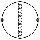
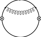
Figure 1: One- and two-loop diagrams contributing to $\Pi^{(0)}$ and $\Pi^{(1)}$, respectively.

For the $\alpha_{s}^{2}$ calculation the diagrams can be decomposed according to the colour structure. The contributions from diagrams with $n_{l}$ light or one massive internal fermion loop will be denoted by $C_{F}Tn_{l}\Pi_{l}$ and $C_{F}T\Pi_{F}$ with the group theoretical coefficients factored out (Figure 2). Purely gluonic corrections (Figure 3) are proportional to $C_{F}^{2}$ or $C_{F}C_{A}$. The former are the only contributions in an Abelian theory, the latter are characteristic for the non-Abelian aspects of QCD. It will be important in the subsequent discussion to treat these two classes separately, since they exhibit strikingly different behaviour close to threshold. The following decomposition of $\Pi(q^{2})$ is therefore adopted throughout the paper

$$\Pi = \Pi^{(0)}+\frac{\alpha_{s}(\mu^{2})}{\pi}C_{F}\Pi^{(1)}$$ (11)

$$+\left(\frac{\alpha_{s}(\mu^{2})}{\pi}\right)^{2}\left[C_{F}^{2}\Pi_{A}^{(2)}+C_{A}C_{F}\Pi_{\it NA}^{(2)}+C_{F}Tn_{l}\Pi_{l}^{(2)}+C_{F}T\Pi_{F}^{(2)}\right].$$

All steps described below will be performed separately for the first three $\Pi^{(2)}$. In fact, new information will only be obtained for $\Pi_{A}^{(2)}$ and $\Pi_{\it NA}^{(2)}$. The imaginary part of $\mbox{Im}\Pi_{l}^{(2)}$ is known analytically already [10]. $\mbox{Im}\Pi_{F}^{(2)}$ can easily be calculated numerically for the following reasons: The amplitude with a massive internal fermion exhibits a two particle cut with threshold at $2m$ which can be calculated analytically [10] and a four particle cut with threshold at $4m$ which is given in terms of a two dimensional integral [10] which can be solved easily numerically. This contribution is therefore known already and will not be treated in this paper.

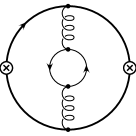
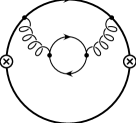
Figure 2: Three-loop diagrams contributing to $\Pi^{(2)}_{l}$ (inner quark massless) and $\Pi_{F}^{(2)}$ (both quarks have the same mass $m$).

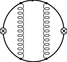
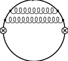
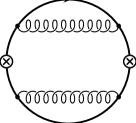
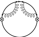
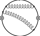
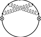
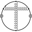
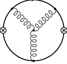
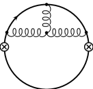
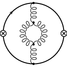
Figure 3: Purely gluonic contribution to ${\cal O}(\alpha_{s}^{2})$. Diagrams with ghost loops are not depicted.

For convenience of the reader we give in the remaining part of this introduction a short description of the individual steps of the calculation.

A crucial input for our procedure is the behaviour of $\Pi(q^{2})$ for $q^{2}\to-\infty$. In Section 3 we list the terms of order $(m^{2}/q^{2})^{0}$ and $(m^{2}/q^{2})^{1}$ for $\Pi^{(2)}$ in the $\overline{\mbox{MS}}$ and on-shell scheme. A very important test for the correctness of the result is provided by the $m^{4}/s^{2}$ terms which are only known for $R(s)$, i.e. the imaginary part of $\Pi$.

In Section 4 we discuss the behaviour of $\Pi(q^{2})$ at threshold. For the QED-like corrections the leading $1/v$ singularities are resummed via Sommerfeld’s formula: $R^{v}=3vx_{s}/2(1-e^{-x_{s}})$ with $x_{s}=C_{F}\pi\alpha_{s}/v$. An expansion up to ${\cal O}(\alpha_{s}^{2})$ delivers the leading singularity for $\Pi_{A}^{(2)}(q^{2}\to 4m^{2})$ and in combination with the “hard” one-loop vertex correction also the subleading logarithmic contribution. With the interpretation of $\alpha_{s}$ in $R^{v}$ as $\alpha_{V}(4\vec{p}\,^{2})$, with $\vec{p}$ being is the momentum of one quark, Eq. (9) reproduces on one side the known threshold term for $R_{l}^{(2)}$ and leads on the other side to an expression for the leading logarithm of $R_{\it NA}^{(2)}$.

Important information is contained in the Taylor series of $\Pi(q^{2})$ around zero. The first seven nontrivial terms are computed. The calculation is based on the evaluation of three-loop tadpole integrals which is performed with the program package MATAD written in FORM [19]. In Section 5 we describe the method in more detail and present our results.

Section 6 is devoted to a discussion of the scheme dependence of the polarization function as well as to a related question of the connection between the QED coupling constant $\alpha$ in the on-shell and the $\overline{\mbox{MS}}$ scheme. We explicitly derive the connection up to and including the terms of order $\alpha^{2}\alpha_{s}^{2}$ using the results of the previous section.

Section 7 contains a description of the procedure which combines the results from the different kinematical regions. In a first step a function with a nonsingular behaviour at high energies is constructed from the known information about $\Pi(q^{2})$. Also the logarithms at threshold are subtracted. The remaining $1/v$ singularity for $\Pi_{A}^{(2)}$ will be removed by multiplication with $v$. The conformal mapping $z=4\omega/(1+\omega)^{2}$ of the complex $q^{2}$-plane into the interior of the unit circle provides a good starting point for the Padé approximation method. The different Padé approximants are denoted by $[n/m]$ and are rational functions with a polynomial of degree $n$ in the numerator and $m$ in the denominator.

The results are discussed and explicit formulae and handy approximations for $R_{A}$ and $R_{\it NA}$ are given in Section 8. Section 9 finally contains our conclusions.

3 Large $q^{2}$ Behaviour

The expansion of $\Pi(q^{2})$ for large $q^{2}$ provides an important constraint on $\Pi$ in the entire complex plane. For the imaginary part it has been argued [5] that the inclusion of the constant, plus quadratic plus quartic terms in $m$ provides an adequate approximation down to fairly close to threshold. The large $q^{2}$ expansion of $\Pi(q^{2})$ reads as follows (The terms proportional to $C_{F}T$ are listed for completeness.):

$$\Pi^{(0)} = \frac{3}{16\pi^{2}}\Bigg{[}\frac{20}{9}-\frac{4}{3}\ln\frac{-q^{2}}{m^{2}}+8\frac{m^{2}}{q^{2}}+\left(\frac{4m^{2}}{q^{2}}\right)^{2}\left(\frac{1}{4}+\frac{1}{2}\ln\frac{-q^{2}}{m^{2}}\right)+\ldots\Bigg{]},$$ (12)

$$\Pi^{(1)} = \frac{3}{16\pi^{2}}\Bigg{[}\frac{5}{6}-4\zeta(3)-\ln\frac{-q^{2}}{m^{2}}-12\frac{m^{2}}{q^{2}}\ln\frac{-q^{2}}{m^{2}}$$ (13)

$$+\left(\frac{4m^{2}}{q^{2}}\right)^{2}\left(\frac{1}{24}+\zeta(3)-\frac{5}{8}\ln\frac{-q^{2}}{m^{2}}-\frac{3}{4}\ln^{2}\frac{-q^{2}}{m^{2}}\right)+\ldots\Bigg{]},$$

$$\Pi_{A}^{(2)} = \frac{3}{16\pi^{2}}\Bigg{[}-\frac{121}{48}-5\zeta(2)+8\zeta(2)\ln 2-\frac{99}{16}\zeta(3)+10\zeta(5)+\frac{1}{8}\ln\frac{-q^{2}}{m^{2}}$$ (14)

$$+\frac{4m^{2}}{q^{2}}\left(\frac{139}{12}-\frac{15}{2}\zeta(2)+12\zeta(2)\ln 2-\frac{41}{12}\zeta(3)-\frac{35}{6}\zeta(5)\right.$$

$$\left.-\frac{3}{8}\ln\frac{-q^{2}}{m^{2}}+\frac{9}{4}\ln^{2}\frac{-q^{2}}{m^{2}}\right)\Bigg{]}+\ldots,$$

$$\Pi_{\it NA}^{(2)} = \frac{3}{16\pi^{2}}\Bigg{[}\frac{4873}{432}+\frac{4}{3}\zeta(2)-4\zeta(2)\ln 2-\frac{4013}{288}\zeta(3)-\frac{5}{3}\zeta(5)-\frac{157}{36}\ln\frac{-q^{2}}{m^{2}}$$ (15)

$$+\frac{11}{12}\ln\frac{-q^{2}}{\mu^{2}}\ln\frac{-q^{2}}{m^{2}}-\frac{11}{24}\ln^{2}\frac{-q^{2}}{m^{2}}-\frac{55}{72}\ln\frac{-q^{2}}{\mu^{2}}+\frac{11}{3}\zeta(3)\ln\frac{-q^{2}}{\mu^{2}}$$

$$+\frac{4m^{2}}{q^{2}}\left(\frac{7}{2}+2\zeta(2)-6\zeta(2)\ln 2+\frac{17}{6}\zeta(3)-\frac{85}{12}\zeta(5)\right.$$

$$\left.-\frac{185}{24}\ln\frac{-q^{2}}{m^{2}}+\frac{11}{4}\ln\frac{-q^{2}}{\mu^{2}}\ln\frac{-q^{2}}{m^{2}}-\frac{11}{8}\ln^{2}\frac{-q^{2}}{m^{2}}\right)\Bigg{]}+\ldots,$$

$$\Pi_{l}^{(2)} = \frac{3}{16\pi^{2}}\Bigg{[}-\frac{116}{27}+\frac{4}{3}\zeta(2)+\frac{38}{9}\zeta(3)+\frac{14}{9}\ln\frac{-q^{2}}{m^{2}}-\frac{1}{3}\ln\frac{-q^{2}}{\mu^{2}}\ln\frac{-q^{2}}{m^{2}}$$ (16)

$$+\frac{1}{6}\ln^{2}\frac{-q^{2}}{m^{2}}+\frac{5}{18}\ln\frac{-q^{2}}{\mu^{2}}-\frac{4}{3}\zeta(3)\ln\frac{-q^{2}}{\mu^{2}}$$

$$+\frac{4m^{2}}{q^{2}}\left(-1+2\zeta(2)+\frac{13}{6}\ln\frac{-q^{2}}{m^{2}}-\ln\frac{-q^{2}}{\mu^{2}}\ln\frac{-q^{2}}{m^{2}}+\frac{1}{2}\ln^{2}\frac{-q^{2}}{m^{2}}\right)\Bigg{]}+\ldots,$$

$$\Pi_{F}^{(2)} = \frac{3}{16\pi^{2}}\Bigg{[}-\frac{307}{216}-\frac{8}{3}\zeta(2)+\frac{545}{144}\zeta(3)+\frac{14}{9}\ln\frac{-q^{2}}{m^{2}}-\frac{1}{3}\ln\frac{-q^{2}}{\mu^{2}}\ln\frac{-q^{2}}{m^{2}}$$ (17)

$$+\frac{1}{6}\ln^{2}\frac{-q^{2}}{m^{2}}+\frac{5}{18}\ln\frac{-q^{2}}{\mu^{2}}-\frac{4}{3}\zeta(3)\ln\frac{-q^{2}}{\mu^{2}}+\frac{4m^{2}}{q^{2}}\left(-\frac{10}{3}-4\zeta(2)\right.$$

$$\left.+4\zeta(3)+\frac{13}{6}\ln\frac{-q^{2}}{m^{2}}-\ln\frac{-q^{2}}{\mu^{2}}\ln\frac{-q^{2}}{m^{2}}+\frac{1}{2}\ln^{2}\frac{-q^{2}}{m^{2}}\right)\Bigg{]}+\ldots.$$

(The logarithmic contributions of the $(m^{2}/q^{2})^{0}$ terms were originally obtained in [1], while the constants in $\Pi^{(2)}$ were first published in [2, 3], albeit not in an explicit form. The quadratic mass terms were first found in [21] and later confirmed in [22].) Eqs. (14-16) imply the following contributions to $R$:

$$R^{(0)} = 3\left[1-6\frac{m^{4}}{s^{2}}+\ldots\right],$$ (18)

$$R^{(1)} = 3\left[\frac{3}{4}+9\frac{m^{2}}{s}+\frac{m^{4}}{s^{2}}\left(\frac{15}{2}-18\ln\frac{m^{2}}{s}\right)+\ldots\right],$$ (19)

$$R_{A}^{(2)} = 3\left[-\frac{3}{32}+\frac{m^{2}}{s}\left(\frac{9}{8}+\frac{27}{2}\ln\frac{m^{2}}{s}\right)+\ldots\right],$$ (20)

$$R_{\it NA}^{(2)} = 3\left[\frac{123}{32}-\frac{11}{4}\zeta(3)+\frac{11}{16}\ln\frac{\mu^{2}}{s}+\frac{m^{2}}{s}\left(\frac{185}{8}+\frac{33}{4}\ln\frac{\mu^{2}}{s}\right)+\ldots\right],$$ (21)

$$R_{l}^{(2)} = 3\left[-\frac{11}{8}+\zeta(3)-\frac{1}{4}\ln\frac{\mu^{2}}{s}+\frac{m^{2}}{s}\left(-\frac{13}{2}-3\ln\frac{\mu^{2}}{s}\right)+\ldots\right].$$ (22)

Note that $R^{(2)}_{F}\equiv R^{(2)}_{l}$ if one considers only $m^{0}$ and $m^{2}$ mass corrections. The equality can be understood within the renormalization group approach of [4].

The quartic contributions to $R$ have been obtained in [5]. They will be important for comparisons with the present results and read as follows:

$$R_{A}^{(2)\scriptsize,m^{4}} = 3\frac{m^{4}}{s^{2}}\Bigg{[}-\frac{345}{16}+99\zeta(2)-72\ln 2\zeta(2)+36\zeta(3)$$ (23)

$$+\frac{81}{4}\ln\frac{m^{2}}{s}-27\ln^{2}\frac{m^{2}}{s}\Bigg{]},$$

$$R_{\it NA}^{(2)\scriptsize,m^{4}} = 3\frac{m^{4}}{s^{2}}\Bigg{[}\frac{77}{3}+\frac{9}{2}\zeta(2)+36\ln 2\zeta(2)+11\zeta(3)$$ (24)

$$-\frac{381}{8}\ln\frac{m^{2}}{s}+\frac{33}{4}\ln^{2}\frac{m^{2}}{s}+\frac{55}{8}\ln\frac{\mu^{2}}{s}-\frac{33}{2}\ln\frac{m^{2}}{s}\ln\frac{\mu^{2}}{s}\Bigg{]},$$

$$R_{l}^{(2)\scriptsize,m^{4}} = 3\frac{m^{4}}{s^{2}}\Bigg{[}-\frac{35}{6}-18\zeta(2)-4\zeta(3)$$ (25)

$$+\frac{27}{2}\ln\frac{m^{2}}{s}-3\ln^{2}\frac{m^{2}}{s}-\frac{5}{2}\ln\frac{\mu^{2}}{s}+6\ln\frac{m^{2}}{s}\ln\frac{\mu^{2}}{s}\Bigg{]},$$

$$R_{F}^{(2)\scriptsize,m^{4}} = 3\frac{m^{4}}{s^{2}}\Bigg{[}\frac{2}{3}+18\zeta(2)-10\zeta(3)$$ (26)

$$+12\ln\frac{m^{2}}{s}-3\ln^{2}\frac{m^{2}}{s}-\frac{5}{2}\ln\frac{\mu^{2}}{s}+6\ln\frac{m^{2}}{s}\ln\frac{\mu^{2}}{s}\Bigg{]}.$$

The results have been expressed in terms of the on-shell mass in order to combine them easily with the threshold and low $q^{2}$ behaviour. As can be seen from Eqs. (14), (20) and (23) the Abelian parts of $\Pi^{(2)}$ and $R^{(2)}$ are in this case independent of $\mu$ whereas the $\mu$ dependence of non-Abelian and fermionic contributions is connected to the running of the coupling constant $\alpha_{s}(\mu^{2})$. For completeness the Eqs. (12-17) are reexpressed in terms of the $\overline{\mbox{MS}}$ mass $\bar{m}$:

$$\bar{\Pi}^{(0)} = \frac{3}{16\pi^{2}}\Bigg{[}\frac{20}{9}-\frac{4}{3}\ln\frac{-q^{2}}{\mu^{2}}+8\frac{\bar{m}^{2}}{q^{2}}+\left(\frac{4\bar{m}^{2}}{q^{2}}\right)^{2}\left(\frac{1}{4}+\frac{1}{2}\ln\frac{-q^{2}}{\bar{m}^{2}}\right)+\ldots\Bigg{]},$$ (27)

$$\bar{\Pi}^{(1)} = \frac{3}{16\pi^{2}}\Bigg{[}\frac{55}{12}-4\zeta(3)-\ln\frac{-q^{2}}{\mu^{2}}+\frac{4\bar{m}^{2}}{q^{2}}\left(4-3\ln\frac{-q^{2}}{\mu^{2}}\right)$$ (28)

$$+\left(\frac{4\bar{m}^{2}}{q^{2}}\right)^{2}\left(\frac{1}{24}+\zeta(3)+\frac{11}{8}\ln\frac{-q^{2}}{\bar{m}^{2}}+\frac{3}{4}\ln^{2}\frac{-q^{2}}{\bar{m}^{2}}-\frac{3}{2}\ln\frac{-q^{2}}{\bar{m}^{2}}\ln\frac{-q^{2}}{\mu^{2}}\right)\Bigg{]},$$

$$\bar{\Pi}_{A}^{(2)} = \frac{3}{16\pi^{2}}\Bigg{[}-\frac{143}{72}-\frac{37}{6}\zeta(3)+10\zeta(5)+\frac{1}{8}\ln\frac{-q^{2}}{\mu^{2}}$$ (29)

$$+\frac{4\bar{m}^{2}}{q^{2}}\left(\frac{1667}{96}-\frac{5}{12}\zeta(3)-\frac{35}{6}\zeta(5)-\frac{51}{8}\ln\frac{-q^{2}}{\mu^{2}}+\frac{9}{4}\ln^{2}\frac{-q^{2}}{\mu^{2}}\right)\Bigg{]}+\ldots,$$

$$\bar{\Pi}_{\it NA}^{(2)} = \frac{3}{16\pi^{2}}\Bigg{[}+\frac{44215}{2592}-\frac{227}{18}\zeta(3)-\frac{5}{3}\zeta(5)-\frac{41}{8}\ln\frac{-q^{2}}{\mu^{2}}+\frac{11}{24}\ln^{2}\frac{-q^{2}}{\mu^{2}}+\frac{11}{3}\zeta(3)\ln\frac{-q^{2}}{\mu^{2}}$$ (30)

$$+\frac{4\bar{m}^{2}}{q^{2}}\left(+\frac{1447}{96}+\frac{4}{3}\zeta(3)-\frac{85}{12}\zeta(5)-\frac{185}{24}\ln\frac{-q^{2}}{\mu^{2}}+\frac{11}{8}\ln^{2}\frac{-q^{2}}{\mu^{2}}\right)\Bigg{]}+\ldots,$$

$$\bar{\Pi}_{l}^{(2)} = \frac{3}{16\pi^{2}}\Bigg{[}-\frac{3701}{648}+\frac{38}{9}\zeta(3)+\frac{11}{6}\ln\frac{-q^{2}}{\mu^{2}}-\frac{1}{6}\ln^{2}\frac{-q^{2}}{\mu^{2}}-\frac{4}{3}\zeta(3)\ln\frac{-q^{2}}{\mu^{2}}$$ (31)

$$+\frac{4\bar{m}^{2}}{q^{2}}\left(-\frac{95}{24}+\frac{13}{6}\ln\frac{-q^{2}}{\mu^{2}}-\frac{1}{2}\ln^{2}\frac{-q^{2}}{\mu^{2}}\right)\Bigg{]}+\ldots,$$

$$\bar{\Pi}_{F}^{(2)} = \frac{3}{16\pi^{2}}\Bigg{[}-\frac{3701}{648}+\frac{38}{9}\zeta(3)+\frac{11}{6}\ln\frac{-q^{2}}{\mu^{2}}-\frac{1}{6}\ln^{2}\frac{-q^{2}}{\mu^{2}}-\frac{4}{3}\zeta(3)\ln\frac{-q^{2}}{\mu^{2}}$$ (32)

$$+\frac{4\bar{m}^{2}}{q^{2}}\left(-\frac{223}{24}+4\zeta(3)+\frac{13}{6}\ln\frac{-q^{2}}{\mu^{2}}-\frac{1}{2}\ln^{2}\frac{-q^{2}}{\mu^{2}}\right)\Bigg{]}+\ldots.$$

4 Threshold Behaviour

The constraints on the threshold behaviour of $\Pi(q^{2})$ originate from our knowledge about the non-relativistic Greens function in the presence of a Coulomb potential and its interplay with “hard” vertex corrections. For a theory with non-vanishing $\beta$ function (QED with light fermions or QCD) the proper definition of the coupling constant and its running must be taken into account.

For completeness let us recall the ${\cal O}(\alpha_{s})$ result. To this order $R(s)$ is known analytically and reads (expressed in the variable $v=\sqrt{1-4m^{2}/s}$):

$$R^{(0)} = 3v\frac{3-v^{2}}{2},$$ (33)

$$R^{(1)} = 3\frac{3-v^{2}}{2}\Bigg{[}(1+v^{2})\left(\mbox{Li}_{2}\left(\left(\frac{1-v}{1+v}\right)^{2}\right)+2\mbox{Li}_{2}\left(\frac{1-v}{1+v}\right)+\ln\frac{1+v}{1-v}\ln\frac{(1+v)^{3}}{8v^{2}}\right)$$ (34)

$$\hphantom{3\frac{3-v^{2}}{2}}+3v\ln\frac{1-v^{2}}{4v}-v\ln v+\frac{33+22v^{2}-7v^{4}}{8(3-v^{2})}\ln\frac{1+v}{1-v}+\frac{15v-9v^{3}}{4(3-v^{2})}\Bigg{]},$$

$$R(s) = R^{(0)}+C_{F}\frac{\alpha_{s}(s)}{\pi}R^{(1)}+{\cal O}(\alpha_{s}^{2})$$ (35)

$$= 3\frac{3}{2}v\left(1+\frac{\alpha_{s}}{\pi}C_{F}\left(\frac{\pi^{2}(1+v^{2})}{2v}-4\right)+{\cal O}(v,\alpha_{s}^{2})\right).$$ (36)

In the last line an expansion for small velocities $v$ is performed. The $\pi^{2}/2v$ term results from longitudinal gluon exchange, the potential, whereas the “$-4$” originates from a transversal, hard gluon.

For the present problem this has to be extended to ${\cal O}(\alpha_{s}^{2})$. Let us in a first step discuss the $C_{F}^{2}$ terms which are relevant for QCD and QED. For convenience everything will be formulated for QED with the trivial translation $\alpha\to C_{F}\alpha_{s}$ implied for QCD. The leading terms in an expansion of $x=\pi\alpha/v$ are given by

$$R^{v} = \frac{3}{2}\frac{vx}{1-e^{-x}}=\frac{3}{2}v\left(1+\frac{x}{2}+\frac{B_{1}x^{2}}{2!}-\frac{B_{2}x^{4}}{4!}+\frac{B_{3}x^{6}}{6!}\pm\ldots+(-1)^{(n+1)}\frac{B_{n}x^{2n}}{(2n)!}\pm\ldots\right)$$ (37)

$$= \frac{3}{2}v\left(1+\frac{\alpha}{\pi}\frac{\pi^{2}}{2v}+\left(\frac{\alpha}{\pi}\right)^{2}\frac{\pi^{4}}{12v^{2}}+\cdots\right)$$

where $B_{n}$ are the Bernoulli numbers: $B_{1}=1/6,\,B_{2}=1/30,\,B_{3}=1/42,\,\ldots$. These terms are induced by rescattering through the Coulomb potential. Formally they are obtained from the imaginary part of the Greens function. In addition there is a correction factor $(1-4\alpha/\pi)$ from transversal photon (gluon) exchange. In QCD this term is quite familiar from the corrections to quarkonium annihilation through a virtual photon [23]. These considerations allow to reconstruct the $1/v$ and the constant term in order $\alpha^{2}$ [15, 24]

$$R_{A}^{(2)} = 3\left(\frac{\pi^{4}}{8v}-3\pi^{2}+\ldots\right).$$ (38)

Now it is possible to define the leading term of $\Pi^{(2)}_{A}$ in such a way that its imaginary part reproduces Eq. (38):

$$\Pi^{(2)}_{A} = \frac{3}{16\pi^{2}}\left(\frac{\pi^{5}}{6\sqrt{1-z}}+4\pi^{2}\ln(1-z)+\ldots\right)$$ (39)

In Ref. [15] this information has been included by considering the combination $\Pi_{A}^{(2)}+4\Pi^{(1)}$ which is free from a logarithmic singularity at $q^{2}=4m^{2}$ and we shall adopt the same strategy.

In the discussion of the terms proportional to $C_{F}Tn_{l}$ and $C_{A}C_{F}$ additional aspects must be taken into consideration if one wants to predict the term of ${\cal O}(\alpha_{s}^{2}v^{0})$ multiplied by powers of logarithms. This is related to the fact that for a prediction of ${\cal O}(\alpha_{s}^{2})$ the definition of the coupling constant, the renormalization scheme and the choice of scale affect the functional dependence of the result. The problem arises already in a discussion of QED with additional $n_{l}$ light fermions. Including purely photonic corrections up to order $\alpha$ and contributions with $n_{l}$ light fermion loops of order $\alpha^{2}$ one obtains in QED close to threshold [10]

$$\!R_{QED}^{thr}\!\! \!=\! \!\!\frac{v(3-v^{2})}{2}\left[1+\frac{\bar{\alpha}(\mu^{2})}{\pi}\frac{\pi^{2}(1+v^{2})}{2v}+n_{l}\left(\frac{\bar{\alpha}(\mu^{2})}{\pi}\right)^{2}\frac{\pi^{2}(1+v^{2})}{6v}\left(\ln\frac{v^{2}s}{\mu^{2}}-\frac{5}{3}\right)\right].$$ (40)

where the $\overline{\mbox{MS}}$ definition of the coupling constant has been adopted and the mass of the light fermions is set to zero. This result is easily interpreted in the context of the QED potential which can be written in the form ($\vec{q}$ denotes the relative momentum, with $\vec{q}=2\vec{p}$ in the case at hand):

$$V_{QED} = -4\pi\frac{\alpha_{V}^{QED}(\vec{q}\,^{2})}{\vec{q}\,^{2}},$$ (41)

$$\alpha_{V}^{QED}(\vec{q}\,^{2}) = \bar{\alpha}(\mu^{2})\left(1+n_{l}\frac{\bar{\alpha}(\mu^{2})}{\pi}\frac{1}{3}\left(\ln\frac{\vec{q}\,^{2}}{\mu^{2}}-\frac{5}{3}\right)\right),$$ (42)

such that

$$R^{thr}_{QED}=\frac{v(3-v^{2})}{2}\left[1+\frac{\alpha_{V}(4\vec{p}\,^{2})}{\pi}\frac{\pi^{2}(1+v^{2})}{2v}\right].$$ (43)

Returning to the $\overline{\mbox{MS}}$ convention and QCD one now reconstructs the leading terms of the real part of $\Pi(q^{2})$ close to threshold

$$\Pi_{l}^{(2),thr} = \frac{3}{16\pi^{2}}\frac{\pi^{2}}{6}\left[1+\frac{2}{3}\left(1-\frac{1}{z}\right)-\frac{1}{3}\left(1-\frac{1}{z}\right)^{2}\right]$$ (44)

$$\hphantom{\frac{\pi^{2}}{6}}\left[-\ln^{2}\frac{1}{1-z}+2\ln\frac{1}{1-z}\left(\ln\frac{4m^{2}}{\mu^{2}}-\frac{5}{3}\right)\right]+c_{l}$$

with an unknown constant term $c_{l}$. This approach can immediately be transferred to QCD, replacing in Eq. (41) $\alpha_{V}^{QED}(\vec{q}\,^{2})$ by $C_{F}\alpha_{V}^{QCD}(4\vec{p}\,^{2})$ and using Eq. (9). Thus for the $C_{A}C_{F}$ contribution we postulate the following threshold terms:

$$R_{\it NA}^{(2),thr} = 3\frac{\pi^{2}}{3}(3-v^{2})(1+v^{2})\left(-\frac{11}{16}\ln\frac{v^{2}s}{\mu^{2}}+\frac{31}{48}\right),$$ (45)

$$\Pi_{\it NA}^{(2),thr} = \frac{3}{16\pi^{2}}\frac{\pi^{2}}{6}\left[1+\frac{2}{3}\left(1-\frac{1}{z}\right)-\frac{1}{3}\left(1-\frac{1}{z}\right)^{2}\right]$$ (46)

$$\hphantom{\frac{\pi^{2}}{6}}\left[\frac{11}{4}\ln^{2}\frac{1}{1-z}+8\ln\frac{1}{1-z}\left(-\frac{11}{16}\ln\frac{4m^{2}}{\mu^{2}}+\frac{31}{48}\right)\right]+c_{\it NA}.$$

Because $R_{l}^{(2)}$ and $R_{\it NA}^{(2)}$ develop only a logarithmic singularity for $v\to 0$ it is not possible to determine the leading real part completely, i.e. $c_{l}$ and $c_{\it NA}$ in (44) and (46) remain unknown.

5 Small $q^{2}$ Behaviour

The first seven coefficients of the Taylor series around $q^{2}=0$ are calculated with the help of the program MATAD which has been used previously for the three-loop corrections to the $\rho$ parameter [25], to $\Delta r$ [26] and the top loop induced reaction $e^{+}e^{-}\to Hl^{+}l^{-}$ [27]. The package is written in FORM [19]. For a given diagram it performs the derivatives with respect to the external momentum $q^{2}$ to the desired order, raising internal propagators to powers up to about 20. It then performs the traces and uses recurrence relations based on the integration by parts method [28, 29] to reduce the resulting three-loop tadpole diagrams (in dimensional regularisation). We find

$$\Pi^{(0)} = \frac{3}{16\pi^{2}}\left(\frac{16}{15}z+\frac{16}{35}z^{2}+\frac{256}{945}z^{3}+\frac{128}{693}z^{4}+\frac{2048}{15015}z^{5}+\frac{2048}{19305}z^{6}+\frac{65536}{765765}z^{7}+\ldots\right),$$

$$\Pi^{(1)} = \frac{3}{16\pi^{2}}\left(\frac{328}{81}z+\frac{1796}{675}z^{2}+\frac{999664}{496125}z^{3}+\frac{207944}{127575}z^{4}+\frac{1729540864}{1260653625}z^{5}\right.$$

$$+ \left.\frac{21660988864}{18261468225}z^{6}+\frac{401009026048}{383490832725}z^{7}+\ldots\right),$$

$$\Pi^{(2)} = \frac{3}{16\pi^{2}}\sum_{n>0}C_{n}^{(2)}z^{n},$$ (47)

$$C_{1}^{(2)} = C_{F}^{2}\left(-\frac{8687}{864}+4\zeta(2)-\frac{32}{5}\zeta(2)\ln 2+\frac{22781}{1728}\zeta(3)\right)+C_{A}C_{F}\left(\frac{127}{192}+\frac{902}{243}\ln\frac{\mu^{2}}{m^{2}}\right.$$

$$- \left.\frac{16}{15}\zeta(2)+\frac{16}{5}\zeta(2)\ln 2+\frac{1451}{384}\zeta(3)\right)+C_{F}Tn_{l}\left(-\frac{142}{243}-\frac{328}{243}\ln\frac{\mu^{2}}{m^{2}}-\frac{16}{15}\zeta(2)\right)$$

$$+ C_{F}T\left(-\frac{11407}{2916}-\frac{328}{243}\ln\frac{\mu^{2}}{m^{2}}+\frac{32}{15}\zeta(2)+\frac{203}{216}\zeta(3)\right),$$

$$C_{2}^{(2)} = C_{F}^{2}\left(-\frac{223404289}{1866240}+\frac{24}{7}\zeta(2)-\frac{192}{35}\zeta(2)\ln 2+\frac{4857587}{46080}\zeta(3)\right)$$

$$+ C_{A}C_{F}\left(-\frac{1030213543}{93312000}+\frac{4939}{2025}\ln\frac{\mu^{2}}{m^{2}}-\frac{32}{35}\zeta(2)+\frac{96}{35}\zeta(2)\ln 2+\frac{723515}{55296}\zeta(3)\right)$$

$$+ C_{F}Tn_{l}\left(-\frac{40703}{60750}-\frac{1796}{2025}\ln\frac{\mu^{2}}{m^{2}}-\frac{32}{35}\zeta(2)\right)$$

$$+ C_{F}T\left(-\frac{1520789}{414720}-\frac{1796}{2025}\ln\frac{\mu^{2}}{m^{2}}+\frac{64}{35}\zeta(2)+\frac{14203}{18432}\zeta(3)\right),$$

$$C_{3}^{(2)} = C_{F}^{2}\left(-\frac{885937890461}{1161216000}+\frac{64}{21}\zeta(2)-\frac{512}{105}\zeta(2)\ln 2+\frac{33067024499}{51609600}\zeta(3)\right)$$

$$+ C_{A}C_{F}\left(-\frac{95905830011197}{1706987520000}+\frac{2749076}{1488375}\ln\frac{\mu^{2}}{m^{2}}-\frac{256}{315}\zeta(2)+\frac{256}{105}\zeta(2)\ln 2\right.$$

$$+ \left.\frac{5164056461}{103219200}\zeta(3)\right)+C_{F}Tn_{l}\left(-\frac{9703588}{17364375}-\frac{999664}{1488375}\ln\frac{\mu^{2}}{m^{2}}-\frac{256}{315}\zeta(2)\right)$$

$$+ C_{F}T\left(-\frac{83936527}{23328000}-\frac{999664}{1488375}\ln\frac{\mu^{2}}{m^{2}}+\frac{512}{315}\zeta(2)+\frac{12355}{13824}\zeta(3)\right),$$

$$C_{4}^{(2)} = C_{F}^{2}\left(-\frac{269240669884818833}{61451550720000}+\frac{640}{231}\zeta(2)-\frac{1024}{231}\zeta(2)\ln 2+\frac{1507351507033}{412876800}\zeta(3)\right)$$

$$+ C_{A}C_{F}\left(-\frac{36675392331131681}{158018273280000}+\frac{571846}{382725}\ln\frac{\mu^{2}}{m^{2}}-\frac{512}{693}\zeta(2)+\frac{512}{231}\zeta(2)\ln 2\right.$$

$$+ \left.\frac{1455887207647}{7431782400}\zeta(3)\right)+C_{F}Tn_{l}\left(-\frac{54924808}{120558375}-\frac{207944}{382725}\ln\frac{\mu^{2}}{m^{2}}-\frac{512}{693}\zeta(2)\right)$$

$$+ C_{F}T\left(-\frac{129586264289}{35831808000}-\frac{207944}{382725}\ln\frac{\mu^{2}}{m^{2}}+\frac{1024}{693}\zeta(2)+\frac{2522821}{2359296}\zeta(3)\right),$$

$$C_{5}^{(2)} = C_{F}^{2}\left(-\frac{360248170450504167133}{15209258803200000}+\frac{2560}{1001}\zeta(2)-\frac{4096}{1001}\zeta(2)\ln 2\right.$$

$$+ \left.\frac{939939943788973}{47687270400}\zeta(3)\right)+C_{A}C_{F}\left(-\frac{21883348499544169357}{23658847027200000}\right.$$

$$+ \left.\frac{432385216}{343814625}\ln\frac{\mu^{2}}{m^{2}}-\frac{2048}{3003}\zeta(2)+\frac{2048}{1001}\zeta(2)\ln 2+\frac{14724562345079}{19074908160}\zeta(3)\right)$$

$$+ C_{F}Tn_{l}\left(-\frac{4881989801536}{13104494431875}-\frac{1729540864}{3781960875}\ln\frac{\mu^{2}}{m^{2}}-\frac{2048}{3003}\zeta(2)\right)$$

$$+ C_{F}T\left(-\frac{512847330943}{139087872000}-\frac{1729540864}{3781960875}\ln\frac{\mu^{2}}{m^{2}}+\frac{4096}{3003}\zeta(2)+\frac{1239683}{983040}\zeta(3)\right),$$

$$C_{6}^{(2)} = C_{F}^{2}\left(-\frac{64959156551995419148501103}{529285210649395200000}+\frac{1024}{429}\zeta(2)-\frac{8192}{2145}\zeta(2)\ln 2\right.$$

$$+ \left.\frac{330704075360938001}{3238841548800}\zeta(3)\right)+C_{A}C_{F}\left(-\frac{4826864658245605658856745531}{1317342772469012889600000}\right.$$

$$+ \left.+\frac{5415247216}{4980400425}\ln\frac{\mu^{2}}{m^{2}}-\frac{4096}{6435}\zeta(2)+\frac{4096}{2145}\zeta(2)\ln 2+\frac{580922571682067161}{190443883069440}\zeta(3)\right)$$

$$+ C_{F}Tn_{l}\left(-\frac{151249070952032}{493552701717075}-\frac{21660988864}{54784404675}\ln\frac{\mu^{2}}{m^{2}}-\frac{4096}{6435}\zeta(2)\right)$$

$$+ C_{F}T\left(-\frac{3411069430668887863}{899847347503104000}-\frac{21660988864}{54784404675}\ln\frac{\mu^{2}}{m^{2}}+\frac{8192}{6435}\zeta(2)\right.$$

$$+ \left.\frac{1760922667}{1207959552}\zeta(3)\right),$$

$$C_{7}^{(2)} = C_{F}^{2}\left(-\frac{571365897351090627148045413923471}{927409311818185074278400000}+\frac{16384}{7293}\zeta(2)-\frac{131072}{36465}\zeta(2)\ln 2\right.$$

$$+ \left.\frac{13386367971827490465799}{26118018249523200}\zeta(3)\right)$$

$$+ C_{A}C_{F}\left(-\frac{7342721436809271685822267340249}{505859624628100949606400000}+\frac{100252256512}{104588408925}\ln\frac{\mu^{2}}{m^{2}}\right.$$

$$- \left.\frac{65536}{109395}\zeta(2)+\frac{65536}{36465}\zeta(2)\ln 2+\frac{14019414333929589373}{1160800811089920}\zeta(3)\right)$$

$$+ C_{F}Tn_{l}\left(-\frac{13125091764358528}{51823033680292875}-\frac{401009026048}{1150472498175}\ln\frac{\mu^{2}}{m^{2}}-\frac{65536}{109395}\zeta(2)\right)$$

$$+ C_{F}T\left(-\frac{7927736038867601807}{2024656531881984000}-\frac{401009026048}{1150472498175}\ln\frac{\mu^{2}}{m^{2}}+\frac{131072}{109395}\zeta(2)\right.$$

$$+ \left.\frac{4497899939}{2717908992}\zeta(3)\right).$$

The coefficients $C_{1}^{(2)}-C_{4}^{(2)}$ were already presented in [11], $C_{5}^{(2)},C_{6}^{(2)}$ and $C_{7}^{(2)}$ are new. The $C_{F}^{2}$ term of $C_{1}^{(2)}-C_{3}^{(2)}$ and $C_{5}^{(2)}$ are in agreement with [15] and [30], respectively.

The $\mu$ dependence of the terms proportional to $C_{A}C_{F}$ and $C_{F}Tn_{l}$ is again due to the running of $\alpha_{s}(\mu^{2})$. If the $\overline{\mbox{MS}}$ definition of the mass is used, the Abelian part also develops a $\mu$ dependence — a consequence of the anomalous mass dimension — and in general $\ln^{2}\mu^{2}$ terms appear. The corresponding expressions can easily be derived using Eq. (7) and will not be listed. Instead we want to apply the BLM procedure [31] to our results.

n	$C_{n}^{(0)}$	$C_{n}^{(1)}$	$C_{A,n}^{(2)}$	$C_{{\it NA},n}^{(2)}$	$C_{l,n}^{(2)}$	$C_{n}^{(2)}$	$C_{n}^{BLM}$	$\mu_{BLM}/m$	$\bar{C}_{n}^{(1)}$	$\bar{C}_{n}^{(2)}$
1	1.07	4.05	5.08	7.10	-2.34	30.1	13.7	0.420	1.92	3.82
2	0.46	2.66	6.39	6.31	-2.17	29.5	14.3	0.294	0.83	3.69
3	0.27	2.01	6.69	5.40	-1.90	27.3	14.0	0.244	0.39	2.50
4	0.18	1.63	6.68	4.70	-1.67	25.2	13.5	0.215	0.15	1.65
5	0.14	1.37	6.57	4.16	-1.49	23.4	13.0	0.195	0.01	1.12
6	0.11	1.19	6.43	3.75	-1.35	21.9	12.5	0.181	-0.09	0.85
7	0.09	1.05	6.27	3.41	-1.24	20.7	12.0	0.169	-0.15	0.76

Table 1: The BLM scale $\mu_{BLM}$ is expressed in terms of the original scale $m$. For the numerical values of $C_{n}^{(2)}$ and $\bar{C}_{n}^{(2)}$ $n_{l}=5$ and $\mu^{2}=m^{2}$, respectively, $\mu^{2}=\bar{m}^{2}$ is used. The double bubble diagrams with two massive fermion loops are also included. $C_{n}^{BLM}$ is the coefficient remaining after the $\beta_{0}$ term is absorbed.

It suggests to choose the scale of the ${\cal O}(\alpha_{s})$ term in such a way that the contribution of the ${\cal O}(\alpha_{s}^{2})$ part proportional to $\beta_{0}$ is absorbed. This prescription is based on the observation that the remaining coefficients of the $\alpha_{s}^{2}$ terms are often relatively small. It is possible to treat each term of ${\cal O}(z^{n})$ separately. In Table 1 we list the BLM scale $\mu_{BLM}$ for each Taylor coefficient together with the numerical value of the original ($C_{n}^{(2)}$) and the ${\cal O}(\alpha_{s}^{2})$ term which remains after the BLM scale is adjusted ($C_{n}^{BLM}$). It is interesting to note that $\mu_{BLM}$ is decreasing with increasing $n$. This is plausible because the higher Taylor coefficients are increasingly dominated by the threshold region and the characteristic scale at threshold is the relative three-momentum of the quarks. Note that $C_{n}^{BLM}$ remains nearly constant whereas $C_{n}^{(2)}$ decreases for increasing $n$ (but remember the rapidly decreasing coefficients $C_{n}^{(0)}$).

In comparison to $C_{n}^{(2)}$ in Table 1 also the corresponding one- and two-loop coefficients ($C_{n}^{(0)},C_{n}^{(1)}$) and the two- and three-loop coefficients ($\bar{C}_{n}^{(1)},\bar{C}_{n}^{(2)}$) in the $\overline{\mbox{MS}}$ scheme are listed. Whereas $C_{n}^{(1)}$ is roughly of ${\cal O}(1)$ $\bar{C}_{n}^{(1)}$ varies from approximately $1.9$ down to $0.01$. Also the sign changes. Therefore the BLM procedure is rather unstable and not applicable. On the other hand, the $\overline{\mbox{MS}}$ coefficients $\bar{C}_{n}^{(2)}$ are already reasonably small, so there is no urgent need for an optimization procedure.

Using Eq. (9) it is possible to transform $\alpha_{s}(\mu^{2})$ into $\alpha_{V}(\mu^{2})$, which is based on a physical definition. We observed that the quantities $C_{n}^{V}$ are already smaller than the corresponding on-shell ones (but still much larger than in the $\overline{\mbox{MS}}$ scheme). After application of the BLM prescription, however, the coefficients are larger than the corresponding $C_{n}^{BLM}$. No significant reduction of the coefficients is achieved.

6 The QED Coupling Constant in the $\overline{\mbox{MS}}$ Scheme

The vacuum polarization is connected with the physical cross section through the dispersion relation:

$$\Pi(q^{2}) = \frac{q^{2}}{12\pi^{2}}\int_{4m^{2}}^{\infty}\,ds\,\,\frac{R(s)}{s(s-q^{2})}+\frac{3}{16\pi^{2}}\,C_{0}.$$ (48)

As is well known $\Pi(q^{2})$ by itself is not a physical quantity. This is reflected by the presence of an arbitrary subtraction constant $C_{0}$ in Eq. (48). In QED usually the condition

$$\Pi(0) = 0$$ (49)

is adopted which obviously leads to $C_{0}=0$. Then the photon propagator

$$D(q) = \frac{1}{q^{2}}\frac{1}{1+e^{2}\Pi(q^{2})}$$ (50)

gets canonically normalized in the vicinity of the photon pole $q^{2}\approx 0$ and the electromagnetic charge $e$ coincides with the one defined in the Thompson limit. On the other hand, using the $\overline{\mbox{MS}}$ scheme to renormalize the vacuum polarization function, the photon propagator looks like

$$\bar{D}(q) = \frac{1}{q^{2}}\frac{1}{1+\bar{e}^{2}\bar{\Pi}(q^{2})},$$ (51)

which leads to

$$\alpha = \frac{\bar{\alpha}}{1+\bar{e}^{2}\bar{\Pi}(q^{2}=0)}\,=\,\frac{\bar{\alpha}}{1+\frac{3\bar{\alpha}}{4\pi}\bar{C}_{0}}.$$ (52)

This relation is not well defined if one takes into account massless quark contributions to $\Pi$ (even within perturbation theory), but it correctly describes the part of the relation between on-shell and $\overline{\mbox{MS}}$ electromagnetic coupling constant coming from a massive quark coupled to the electromagnetic current. For a sufficiently heavy quark this relation could even be used for a reliable theoretical estimation of the quark contribution to the charge renormalization. The Taylor series for the vacuum polarization discussed in the previous section was evaluated in a first step in the $\overline{\mbox{MS}}$ scheme, with a constant term given by

$$\frac{16\pi^{2}}{3}\bar{\Pi}(0)\,\,=\,\,\bar{C}_{0}\,\,=\,\,$$ (53)

$$\frac{4}{3}\ln\frac{\mu^{2}}{m^{2}}+\frac{\alpha_{s}(\mu^{2})}{\pi}C_{F}\left(\frac{15}{4}+\ln\frac{\mu^{2}}{m^{2}}\right)+\left(\frac{\alpha_{s}(\mu^{2})}{\pi}\right)^{2}\Bigg{[}$$

$$C_{F}^{2}\left(\frac{77}{144}-\frac{1}{8}\ln\frac{\mu^{2}}{m^{2}}+5\zeta(2)-8\zeta(2)\ln 2+\frac{1}{48}\zeta(3)\right)$$

$$+C_{A}C_{F}\left(\frac{14977}{2592}+\frac{157}{36}\ln\frac{\mu^{2}}{m^{2}}+\frac{11}{24}\ln^{2}\frac{\mu^{2}}{m^{2}}-\frac{4}{3}\zeta(2)+4\zeta(2)\ln 2+\frac{127}{96}\zeta(3)\right)$$

$$+C_{F}TN_{f}\left(-\frac{917}{648}-\frac{14}{9}\ln\frac{\mu^{2}}{m^{2}}-\frac{1}{6}\ln^{2}\frac{\mu^{2}}{m^{2}}-\frac{4}{3}\zeta(2)\right)$$

$$+C_{F}T\left(-\frac{23}{8}+4\zeta(2)+\frac{7}{16}\zeta(3)\right)\Bigg{]}.$$

This leads to the following relation between $\alpha$ and $\bar{\alpha}(\mu^{2})$:

$$\alpha = \bar{\alpha}(\mu^{2})\left[1-\frac{3\bar{\alpha}(\mu^{2})}{4\pi}\bar{C}_{0}\right],$$ (54)

$$\bar{\alpha}(\mu^{2}) = \alpha\left[1+\frac{3\alpha}{4\pi}\bar{C}_{0}\right].$$ (55)

For the QED case (i.e. $C_{F}=1,C_{A}=0,T=1/2$ and $N_{f}=1$) the result of [29] is reproduced.

7 Optimized Approximation

It is evidently a promising strategy to construct, in a first step, a function $\tilde{\Pi}(q^{2})$ whose discontinuity across the cut approximates the one of the full vacuum polarization up to subleading terms — in other words, which exhibits a similar spectral function. The approximation will have different structure for $\Pi_{A}$ on one side and $\Pi_{\it NA}$ and $\Pi_{l}$ on the other side as a consequence of their different threshold singularities.

For the following discussion the on-shell scheme for the mass $m$ is used and the ’t Hooft mass $\mu^{2}$ is set to $m^{2}$. For the $C_{F}^{2}$ term we proceed as in [15] and define $\tilde{\Pi}_{A}$ as follows:

$$\tilde{\Pi}_{A}^{(2)}(q^{2}) = \Pi_{A}^{(2)}(q^{2})+4\Pi^{(1)}(q^{2})$$ (56)

$$+\frac{3}{16\pi^{2}}\Bigg{[}(1-z)G(z)\left(9G(z)+\frac{229+62z}{8z}\right)-\frac{229}{8z}-\frac{173}{24}\Bigg{]}.$$

As already mentioned above the combination $\Pi_{A}^{(2)}(q^{2})+4\Pi^{(1)}(q^{2})$ is free of logarithmic singularities at threshold whereas the $1/v$ term remains and is treated below. The high energy logarithms have to be removed in such a way that the threshold behaviour and the polynomial structure for $q^{2}\to 0$ is not destroyed. Therefore we use the function $G(z)$ which is essentially the result in the one-loop case. The terms quadratic in $G(z)$ remove the $1/z\ln^{2}(-z)$ terms whereas the linear ones develop only single logarithms for $q^{2}\to-\infty$. The factor $(1-z)$ ensures that the threshold is not touched. The last two terms reestablish the condition that the new polarization function also vanishes for $q^{2}=0$.

In a next step we map the complex $q^{2}$-plane into the interior of the unit circle with the help of the variable transformation [32]

$$\omega=\frac{1-\sqrt{1-q^{2}/4m^{2}}}{1+\sqrt{1-q^{2}/4m^{2}}},\,\,\,\, \frac{q^{2}}{4m^{2}}=\frac{4\omega}{(1+\omega)^{2}}.$$ (57)

The special points $q^{2}=0,4m^{2},-\infty$ correspond to $\omega=0,1,-1$, respectively. In Figure 4 this conformal mapping is visualized. The upper (lower) part of the cut form $z=1$ to $\infty$ is mapped onto the upper (lower) perimeter of the circle. The Taylor series which in the variable $z$ only converges for $|q^{2}|<4m^{2}$ is now convergent in the interior of the unit circle in the complex $\omega$ plane.

Figure 4: Transformation between the $z$ and $\omega$ plane

To improve the approximation in a way which allows to approach the boundary of the domain of analycity it has been suggested to use Padé approximations. Following [15] we define

$$P_{A}(\omega) = \frac{1-\omega}{(1+\omega)^{2}}\left[\tilde{\Pi}_{A}^{(2)}(q^{2})-\tilde{\Pi}_{A}^{(2)}(-\infty)\right].$$ (58)

The knowledge of $\tilde{\Pi}_{A}^{(2)}(q^{2})$ in the three different kinematical regions translates into information for $P(\omega)$ for $\omega=-1,0$ and $1$. Due to the fact that $P^{\prime}(-1)=0$ (this is because of the definition of $\omega$) the constant term in the high energy limit, $\tilde{\Pi}_{A}^{(2)}(-\infty)$, is subtracted. The factor $1/(1+\omega)^{2}$ then guarantees that in the limit $\omega\to-1$ the power suppressed term of $\tilde{\Pi}_{A}^{(2)}(q^{2})$ is projected out whereas the factor $(1-\omega)$ together with the $1/v$-singularity of $\tilde{\Pi}(q^{2})$ results in a finite value for $P(1)$. For the construction of the Padé approximants the following information about $P_{A}(\omega)$ is available: $\{P_{A}(-1),P_{A}(0),P_{A}^{\prime}(0),\ldots,P_{A}^{(7)}(0),P_{A}(1)\}$. These ten data points are enough to construct Padé approximants like $[4/5]$ or $[5/4]$.

The above procedure has to be modified for $\Pi_{\it NA}^{(2)}$ and $\Pi_{l}^{(2)}$ because of the different threshold behaviour. Here the logarithmic singularities of $\Pi_{{\it NA}/l}$ are subtracted before the Padé approximation is performed. Therefore $\tilde{\Pi}_{\it NA}^{(2)}$ and $\tilde{\Pi}_{l}^{(2)}$ looks like

$$\tilde{\Pi}_{\it NA}^{(2)}(q^{2}) = \Pi_{\it NA}^{(2)}(q^{2})$$ (59)

$$-\left[\Pi_{\it NA}^{(2),thr}(q^{2})-c_{\it NA}+\frac{3}{16\pi^{2}}\frac{\pi^{2}}{6}\left(\frac{16}{9}-\frac{11}{12}\ln 4+\frac{1}{z}\left(\frac{31}{18}-\frac{11}{6}\ln 4\right)\right)\right]$$

$$+\frac{3}{16\pi^{2}}\Bigg{[}z(1-z)G(z)\left(\left(\frac{11}{2z}+\frac{11}{6}-\frac{44}{3}\zeta(2)\right)G(z)\right.$$

$$\left.+\frac{1413+738z-\zeta(2)(1024+992z)-\zeta(3)(264+528z)}{72z^{2}}\right)$$

$$-\frac{157}{8z}-\frac{221}{24}+\zeta(2)\left(\frac{128}{9z}+\frac{244}{27}\right)+\zeta(3)\left(\frac{11}{3z}+\frac{55}{9}\right)\Bigg{]},$$

$$\tilde{\Pi}_{l}^{(2)}(q^{2}) = \Pi_{l}^{(2)}(q^{2})$$ (60)

$$-\left[\Pi_{l}^{(2),thr}(q^{2})-c_{\it l}+\frac{3}{16\pi^{2}}\frac{\pi^{2}}{6}\left(-\frac{8}{9}+\frac{1}{3}\ln 4+\frac{1}{z}\left(-\frac{10}{9}+\frac{2}{3}\ln 4\right)\right)\right]$$

$$+\frac{3}{16\pi^{2}}\Bigg{[}z(1-z)G(z)\left(\left(-\frac{2}{z}-\frac{2}{3}+\frac{16}{3}\zeta(2)\right)G(z)\right.$$

$$\left.+\frac{-105-66z+\zeta(2)(128+160z)+\zeta(3)(24+48z)}{18z^{2}}\right)$$

$$+\frac{35}{6z}+\frac{67}{18}+\zeta(2)\left(-\frac{64}{9z}-\frac{176}{27}\right)+\zeta(3)\left(-\frac{4}{3z}-\frac{20}{9}\right)\Bigg{]}.$$

Again the function $G(z)$ is used to get rid of the high energy logarithms. The additional factor $z$ in front of the $(1-z)(G(z))^{2}$ part has to be introduced because of the $\ln^{2}(-z)$ behaviour of $\Pi_{\it NA}^{(2)}$ and $\Pi_{l}^{(2)}$ for $z\to-\infty$. The terms next to $\Pi_{{\it NA}/l}^{(2),thr}$ are needed in order to ensure that $\tilde{\Pi}_{{\it NA}/l}^{(2)}(0)=0$. The mapping function is defined as

$$P_{{\it NA}/l}(\omega) = \frac{1}{(1+\omega)^{2}}\left[\tilde{\Pi}_{{\it NA}/l}^{(2)}(q^{2})-\tilde{\Pi}_{{\it NA}/l}^{(2)}(-\infty)\right]$$ (61)

and besides $P_{{\it NA}/l}(-1)$ and $P_{{\it NA}/l}(0)$ the first seven derivatives for $\omega=0$ are available. Because of the unknown constants $c_{l}$ and $c_{\it NA}$ defined in (44,46) $P(1)$ is not available. This allows the construction of Padé approximants like $[4/4]$ or $[5/3]$.

For the non-Abelian part, $R_{\it NA}^{(2)}$, there is an other possibility to construct an approximation. This second method is based on the observation that for a special choice of the gauge parameter $\xi$ the complete threshold behaviour and the logarithmic divergency for $s\to\infty$ is covered by the gluonic double bubble diagrams given by the last two diagrams of Fig. 3 (together with the corresponding ghost graphs). Recently, exact results for these contributions with arbitrary $\xi$ were presented [33] which are repeated in Appendix B. It is therefore a strong temptation to consider $\Pi_{\it NA}^{(2)}-\Pi_{g}^{(2)}|_{\xi=4}$ from the very beginning. The imaginary part of this difference is already numerically small, vanishes at threshold and has no logarithmic singularity for $s\to\infty$. In analogy to Eq. (59) and (61) we define

$$\tilde{\Pi}_{\it NA}^{g,(2)}(q^{2}) = \Pi_{\it NA}^{(2)}(q^{2})-\Pi_{g}^{(2)}(q^{2})\Big{|}_{\xi=4}+\frac{3}{16\pi^{2}}\Bigg{[}(1-z)G(z)\frac{33+6z}{4z}-\frac{33}{4z}+\frac{5}{4}\Bigg{]},$$ (62)

$$P_{\it NA}^{g}(\omega) = \frac{1}{(1+\omega)^{2}}\left[\tilde{\Pi}_{\it NA}^{g,(2)}(q^{2})-\tilde{\Pi}_{\it NA}^{g,(2)}(-\infty)\right]$$ (63)

and proceed in the same way as above. The coefficients of $\Pi_{g}^{(2)}(q^{2})|_{\xi=4}$ for $q^{2}\to 0$ and the high energy expansion can be calculated from $\Pi_{l}^{(2)}(q^{2})$ using the formula [33] (see also Appendix B)

$$\Pi_{g}^{(2)}(q^{2})\Big{|}_{\xi=4} = -\frac{11}{4}\Pi_{l}^{(2)}(q^{2})-\frac{2}{3}\Pi^{(1)}(q^{2})$$ (64)

in the different kinematical regions.

We have checked that both methods lead to equivalent results. The second method is, however, more appealing and the results presented below are based on the second choice.

8 Results

After the Padé approximation is performed the Eqs. (56,61,63) are inverted and the threshold and high energy terms are reintroduced. Thus real and imaginary parts of $\Pi^{(2)}$ are at hand. Let us subsequently discuss the absorptive part $R^{(2)}$. We choose $\mu^{2}=m^{2}$ throughout the whole discussion.

Figure 5 shows the complete result for $R_{A}$, $R_{\it NA}$ and $R_{l}$ plotted against the velocity $v$ (solid line). This presentation expands the threshold region. The dashed lines represent the high energy and threshold approximations. The curves are dominated by the threshold singularities. In Figure 6 the same results are shown with abscissa $x=2m/\sqrt{s}$. This presentation expands the high energy region. In addition to the quadratic approximations which are incorporated into $R^{(2)}$ also the quartic approximations (Eqs. (23-25)) are plotted. They are evidently very well reproduced by our method. The exact result for $R_{l}$ from [10] is indistinguishable from the curves in Figure 5 and 6. Also different Padé approximants $[5/4],[4/5],[4/4],\ldots$ deliver practically identical results with a variation comparable to the thickness of the lines. Small variations are visible close to threshold after subtraction of the singular and constant term. Figure 7 shows the results of up to ten different Padé approximants. The spread indicates the error of the method. The agreement in the high energy region is even better. In this Figure only those curves are plotted which have no poles inside the unit circle in the $\omega$ plane. Perfect agreement for $R_{l}^{(2)}$ is observed which is even slightly increased if higher order Padé approximants (solid curves) are taken into account. It is hard to detect the exact result which is represented by the dotted line. $R_{\it NA}^{(2)}$ seems to converge to the solid line ($[4/4],[5/3]$ and $[3/5]$) when more moments from small $q^{2}$ are included. The dashed lines are from the $[3/3],[4/2],[2/4]$ and $[3/4]$, the dotted ones from Padé approximants including only $C_{{\it NA},3}^{(2)}$ and $C_{{\it NA},4}^{(2)}$ ($[3/1],[2/2]$ and $[3/2]$). The dash-dotted curve is the [4/3] Padé approximant and has a pole very close to $\omega=1(1.07\ldots)$. For the Abelian part a classification of the different results can be seen: the dashed lines are $[4/2]$ and $[2/4]$, the solid ones $[3/2],[2/3],[5/3],[3/5]$ and $[5/4]$ Padé approximants.

In the following handy approximation formulae for $R_{A}^{(2)}(s)$ and $R_{\it NA}^{(2)}(s)$ are presented. Details can be found in Appendix A. The results read:

$$R_{A}^{(2)} = \frac{(1-v^{2})^{4}}{v}\frac{3\pi^{4}}{8}-4R^{(1)}+v\frac{2619}{64}-v^{3}\frac{2061}{64}+\frac{81}{8}\left(1-v^{2}\right)\ln\frac{1-v}{1+v}$$ (65)

$$-198\left(\frac{m^{2}}{s}\right)^{3/2}\left(v^{4}-2v^{2}\right)^{6}$$

$$+100p^{3/2}(1-p)\left[2.21P_{0}(p)-1.57P_{1}(p)+0.27P_{2}(p)\right],$$

$$R_{\it NA}^{(2)} = R_{g}^{(2)}\Big{|}_{\xi=4}+v\frac{351}{32}-v^{3}\frac{297}{32}$$ (66)

$$-18\left(\frac{m^{2}}{s}\right)^{3/2}\left(v^{4}-2v^{2}\right)^{4}$$

$$+50p^{3/2}(1-p)\left[1.73P_{0}(p)-1.24P_{1}(p)+0.64P_{2}(p)\right],$$

with $p=(1-v)/(1+v)$. The first line of Eq. (65) and (66) consists of the exactly known high energy and threshold contribution, whereas the second and third line represents the numerically small remainder which is plotted in Figures 8 and 9, respectively, together with the result from the Padé approximation.

9 Conclusions and Summary

Real and imaginary parts of the three-loop polarization of heavy quarks have been calculated. These results can be considered as natural extension of results by Källén and Sabry obtained more than four decades ago. At an intermediate step predictions for the moments (up to $n=7$) are obtained which are basic ingredients for our numerical method, and may in addition also be of interest for the evaluation of QCD sum rules involving heavy quarks. The results for the imaginary part allow to predict the cross section in order $\alpha_{s}^{2}$. The Padé approximation leads to fairly stable predictions with a relative uncertainty for the $\alpha_{s}^{2}$ coefficients of at most 5%. The prediction in its present form can be considered as reliable down to fairly small values of $v$, say to values of $x=4/3\pi\alpha_{s}/v$ around $2$. For even smaller values of $v$ the leading terms of the expansion in $x$ have to be resummed. This aspect will be treated in a future publication.

Acknowledgments

We would like to thank A.H. Hoang and T. Teubner for many interesting discussions. Their programs with the analytical results for $R_{\mbox{\scriptsize\it l}}^{(2)}$ were crucial for our tests of the approximation methods. We are grateful to D. Broadhurst for helpful discussions. Comments by S. Brodsky and M. Voloshin on the threshold behaviour are gratefully acknowledged.

Appendix

Appendix A Approximation Formulae

In this appendix handy approximations for $R_{A}^{(2)}(s)$ and $R_{\it NA}^{(2)}(s)$ are derived. We write $R^{(2)}(s)$ for the different colour factors in the form:

$$R_{A}^{(2)}(s) = R_{A}^{(2),ana}+R_{A}^{(2),rem},$$ (A.1)

$$R_{\it NA}^{(2)}(s) = R_{\it NA}^{g,(2),ana}+R_{\it NA}^{g,(2),rem}.$$ (A.2)

$R^{(2),ana}(s)$ contains the analytically known threshold and high energy behaviour and is chosen in such a way that $R^{(2),rem}(s)$ vanishes both at threshold and at the high energies. In the following the explicit form of $R^{(2),ana}$ is presented and the numerical approximation of $R^{(2),rem}$ is discussed.

Let us first consider the $C_{F}^{2}$ part. Taking the imaginary part of Eq. (56) and solving formally for $R_{A}^{(2)}(s)$ we arrive at

$$R_{A}^{(2)}+4R^{(1)} = \tilde{R}_{A}^{(2)}-\hat{R}_{A}^{(2)}$$ (A.3)

$\hat{R}_{A}^{(2)}$ corresponds to the imaginary part of the last term in Eq. (56) and contains the constant and $m^{2}/s$ terms of the l.h.s. in the limit $s\to\infty$; $\tilde{R}_{A}^{(2)}$ starts at ${\cal O}(m^{4}/s^{2})$. Per construction $\tilde{R}_{A}^{(2)}$ has a $1/v$ singularity at threshold which should be subtracted in such way that the high energy behaviour is not disturbed. This is achieved with an additional factor $(1-v^{2})^{4}$ and leads to

$$R_{A}^{(2)} = R_{A}^{(2),rem}+(1-v^{2})^{4}R_{A}^{(2),thr}-4R^{(1)}-\hat{R}_{A}^{(2)}.$$ (A.4)

$$= R_{A}^{(2),rem}+\frac{(1-v^{2})^{4}}{v}\frac{3\pi^{4}}{8}-4R^{(1)}$$

$$+v\frac{2619}{64}-v^{3}\frac{2061}{64}+\frac{81}{8}\left(1-v^{2}\right)\ln\frac{1-v}{1+v}$$

In Figure 8 $R_{A}^{(2),rem}(s)$ is plotted against $p=(1-v)/(1+v)$ for different Padé approximations. The task is now to find an analytically simple formula which describes the behaviour of this remainder as close as possible. A closer look into the result of the Padé approximation shows that an expansion of $R_{A}^{(2),rem}(s)$ for high energies ($p\to 0$) has the form: $R_{A}^{(2),rem}(s)=p^{3/2}(d_{0}+d_{1}p+d_{2}p^{2}+\ldots)$. The appearance of the half-integer exponents is a relic of the method in particular of the variable $\omega$ introduced in Eq. (57). The $p^{3/2}$ term imitates the quartic mass correction which also contain $\ln^{2}m^{2}$ pieces in an excellent way as can be seen from Figure 6. Thus we performed a fit in the variable $p$ using Legendre polynomials $P_{n}(p)$ multiplied by a factor $p^{3/2}(1-p)$ which ensures the zeros at the boundary. In Figure 8 one can see that for $p\to 0$ a fit with a low order polynomial would fail to deliver an acceptable result, so in a first step a suitable (numerical small) term of ${\cal O}(p^{3/2})$ is added to get a curve which can easily be parametrised including terms up to $n=2$. The result reads:

$$R_{A}^{(2),rem}(s) = -198\left(\frac{m^{2}}{s}\right)^{3/2}\left(v^{4}-2v^{2}\right)^{6}$$ (A.5)

$$+100p^{3/2}(1-p)\left[2.21P_{0}(p)-1.57P_{1}(p)+0.27P_{2}(p)\right],$$

and is also shown in Figure 8.

For the non-Abelian part, $R_{\it NA}^{(2)}$, we exploit that the gluonic double bubble is known exactly (see Eqs. (62) and (63)). Proceeding as above leads to the result:

$$R_{\it NA}^{(2)} = R_{\it NA}^{g,(2),rem}+R_{g}^{(2)}\Big{|}_{\xi=4}+v\frac{351}{32}-v^{3}\frac{297}{32},$$ (A.6)

with

$$R_{\it NA}^{g,(2),rem} = -18\left(\frac{m^{2}}{s}\right)^{3/2}\left(v^{4}-2v^{2}\right)^{4}$$ (A.7)

$$+50p^{3/2}(1-p)\left[1.73P_{0}(p)-1.24P_{1}(p)+0.64P_{2}(p)\right].$$

Appendix B Exact Result for Double Bubble Contribution

In this appendix we list for convenience of the reader the exact result of the imaginary part of the fermionic and gluonic double bubble diagram. Following [33] $R_{l}^{(2)}$, respectively, $R_{g}^{(2)}$ may be written as ($x=l,g$)

$$R_{x}^{(2)}(s) = -\frac{1}{3}\left(R_{\infty}^{x}\ln\frac{\mu^{2}}{s}-R^{x}_{0}\right)R^{(1)}+3R_{\infty}^{x}\delta^{(2)},$$ (B.1)

with $R_{0,\infty}^{x}$ being the moments in the $\overline{\mbox{MS}}$ scheme with the results:

$$R_{\infty}^{l} = 1,$$

$$R_{0}^{l} = -\frac{5}{3}+\ln 4,$$

$$R_{\infty}^{g} = -\frac{5}{4}-\frac{3}{8}\xi,$$

$$R_{0}^{g} = \frac{31}{12}-\frac{3}{4}\xi+\frac{3}{16}\xi^{2}+\left(-\frac{5}{4}-\frac{3}{8}\xi\right)\ln 4.$$ (B.2)

$R^{(1)}$ is defined in (34), whereas $\delta^{(2)}$ was originally calculated in [10] and reads:

$$\delta^{(2)}\,=\,-\,\frac{\left(3-{{v}^{2}}\right)\,\left(1+{{v}^{2}}\right)}{6}\,\times\,$$ (B.3)

$$\mbox{}\,\qquad\,\bigg{\{}\,\mbox{Li}_{3}(p)-2\,\mbox{Li}_{3}(1-p)-3\,\mbox{Li}_{3}({p^{2}})-4\,\mbox{Li}_{3}\Big{(}{p\over{1+p}}\Big{)}-5\,\mbox{Li}_{3}(1-{p^{2}})+\frac{11}{2}\,\zeta(3)\,\,$$

$$\mbox{}\,\qquad+\mbox{Li}_{2}(p)\,\ln\Big{(}\frac{4\,\left(1-{{v}^{2}}\right)}{{{v}^{4}}}\Big{)}+2\,\mbox{Li}_{2}({p^{2}})\,\ln\Big{(}\frac{1-{{v}^{2}}}{2\,{{v}^{2}}}\Big{)}+2\,\zeta(2)\,\bigg{[}\,\ln p-\ln\Big{(}\frac{1-{{v}^{2}}}{4\,v}\Big{)}\,\bigg{]}\,\,$$

$$\mbox{}\,\qquad-\frac{1}{6}\,\ln\Big{(}\frac{1+v}{2}\Big{)}\,\bigg{[}\,36\,\ln 2\,\ln p-44\,\ln^{2}p+49\,\ln p\,\ln\Big{(}\frac{1-{{v}^{2}}}{4}\Big{)}+\ln^{2}\Big{(}\frac{1-{{v}^{2}}}{4}\Big{)}\,\bigg{]}\,\,$$

$$\mbox{}\,\qquad-\frac{1}{2}\,\ln p\,\ln v\,\bigg{[}\,36\,\ln 2+21\,\ln p+16\,\ln v-22\,\ln(1-{{v}^{2}})\,\bigg{]}\,\bigg{\}}\,\,$$

$$\mbox{}+\frac{1}{24}\,\bigg{\{}\,(15-6\,{{v}^{2}}-{{v}^{4}})\,\Big{(}\mbox{Li}_{2}(p)+\mbox{Li}_{2}({p^{2}})\Big{)}+3\,(7-22\,{{v}^{2}}+7\,{{v}^{4}})\,\mbox{Li}_{2}(p)\,\,$$

$$\mbox{}\,\qquad-(1-v)\,(51-45\,v-27\,{{v}^{2}}+5\,{{v}^{3}})\,\zeta(2)\,\,$$

$$\mbox{}\,\qquad+\frac{\left(1+v\right)\,\left(-9+33\,v-9\,{{v}^{2}}-15\,{{v}^{3}}+4\,{{v}^{4}}\right)}{v}\,\ln^{2}p\,\,$$

$$\mbox{}\,\qquad+\bigg{[}\,(33+22\,{{v}^{2}}-7\,{{v}^{4}})\,\ln 2-10\,(3-{{v}^{2}})\,(1+{{v}^{2}})\,\ln v\,\,$$

$$\mbox{}\,\qquad\,\qquad\,\qquad-(15-22\,{{v}^{2}}+3\,{{v}^{4}})\,\ln\Big{(}\frac{1-{{v}^{2}}}{4\,{{v}^{2}}}\Big{)}\,\bigg{]}\,\ln p\,\,$$

$$\mbox{}\,\qquad+2\,v\,(3-{{v}^{2}})\,\ln\Big{(}\frac{4\,\left(1-{{v}^{2}}\right)}{{{v}^{4}}}\Big{)}\,\bigg{[}\,\ln v-3\,\ln\Big{(}\frac{1-{{v}^{2}}}{4\,v}\Big{)}\,\bigg{]}\,\,$$

$$\mbox{}\,\qquad+\frac{237-96\,v+62\,{{v}^{2}}+32\,{{v}^{3}}-59\,{{v}^{4}}}{4}\,\ln p-16\,v\,(3-{{v}^{2}})\,\ln\Big{(}\frac{1+v}{4}\Big{)}\,\,$$

$$\mbox{}\,\qquad-2\,v\,(39-17\,{{v}^{2}})\,\ln\Big{(}\frac{1-{{v}^{2}}}{2\,{{v}^{2}}}\Big{)}-\frac{v\,\left(75-29\,{{v}^{2}}\right)}{2}\,\bigg{\}}\,.$$

Figure 5: Complete results plotted against $v=\sqrt{1-4m^{2}/s}$. The high energy approximation includes the $m^{4}/s^{2}$ term.

Figure 6: High energy region ($x=2m/\sqrt{s}$). The complete results (full line) are compared to the high energy approximations including the $m^{2}/s$ (dash-dotted) and the $m^{4}/s^{2}$ (dashed) terms.

Figure 7: Threshold behaviour of the remainder $\delta R^{(2)}$ for three different Padé approximants. (The singular and constant parts around threshold are subtracted.)

Figure 8: The remainder $R_{A}^{(2),rem}$ plotted for different Padé approximants (dashed lines) together with the result of the fit (Eq. (A.5), solid line).

Figure 9: The remainder $R_{\it NA}^{g,(2),rem}$ plotted for different Padé approximants (dashed lines) together with the result of the fit (Eq. (A.7), solid line).

References

-
[1]
K.G. Chetyrkin, A.L. Kataev and F.V. Tkachov,
Phys. Rev. Lett. 85 (1979) 227;
M. Dine and J. Sapirstein, Phys. Rev. Lett. 43 (1979) 668;
W. Celmaster and R.J. Gonsalves, Phys. Rev. Lett. 44 (1980) 560. - [2] S.G. Gorishny, A.L. Kataev and S.A. Larin, Phys. Lett. B 259 (1991) 144.
- [3] L.R. Surguladze and M.A. Samuel, Phys. Rev. Lett. 66 (1991) 560; erratum ibid, 2416.
- [4] K.G. Chetyrkin and J.H. Kühn, Phys. Lett. B 248 (1990) 359.
- [5] K.G. Chetyrkin and J.H. Kühn, Nucl. Phys. B 432 (1994) 337.
-
[6]
G. Källén and A. Sabry, K. Dan. Vidensk. Selsk. Mat.-Fys. Medd.
29 (1955) No. 17,
see also: J. Schwinger, Particles, Sources and Fields, Vol.II, (Addison-Wesley, New York, 1973). -
[7]
A. Djouadi and C. Verzegnassi,
Phys. Lett. B 195 (1987) 265;
A. Djouadi, Nouvo Cim. 100A (1988) 357. - [8] B.A. Kniehl, J.H. Kühn and R.G. Stuart, Phys. Lett. B 214 (1988) 621.
- [9] B.A. Kniehl, Nucl. Phys. B 347 (1990) 65.
- [10] A.H. Hoang, J.H. Kühn and T. Teubner, Nucl. Phys. B 452 (1995) 173.
- [11] K.G. Chetyrkin, J.H. Kühn and M. Steinhauser, Phys. Lett. B 371 (1996) 93.
- [12] J. Fleischer and O.V. Tarasov, Z. Phys. C 64 (1994) 413.
- [13] D.J. Broadhurst, J. Fleischer and O.V. Tarasov, Z. Phys. C 60 (1993) 287.
- [14] D.J. Broadhurst et. al., Phys. Lett. B 329 (1994) 103.
- [15] P.A. Baikov and D.J. Broadhurst, Report Nos. OUT-4102-54, INP-95-13/377 and hep-ph/9504398, to appear in New Computing Techniques in Physics Research IV, (World Scientific, in press).
-
[16]
W.E. Caswell, Phys. Rev. Lett. 33 (1974) 244;
D.R.T. Jones, Nucl. Phys. B 75 (1974) 531;
E.S. Egorian and O.V. Tarasov, Theor. Mat. Fiz. 41 (1979) 26. -
[17]
W. Fischler, Nucl. Phys. B 129 (1977) 157;
A. Billoire, Phys. Lett. B 92 (1980) 343. - [18] A.H. Hoang, M. Jeżabek, J.H. Kühn and T. Teubner, Phys. Lett. B 338 (1994) 330.
- [19] J.A.M. Vermaseren, Symbolic Manipulation with FORM, (Computer Algebra Netherlands, Amsterdam, 1991).
- [20] R. Barbieri and E. Remiddi, Nouvo Cim. 13A (1973) 99.
- [21] S.G. Gorishny, A.L. Kataev and S.A. Larin, Nouvo Cim. 92A (1986) 119.
-
[22]
K.G. Chetyrkin and A. Kwiatkowski, Z. Phys. C 59 (1993) 525;
L.R. Surguladze, Preprint OITS-554 (1994) and hep-ph/9410409. - [23] R. Barbieri, R. Gatto, R. Kögerler and Z. Kunszt, Phys. Lett. B 57 (1975) 455.
- [24] B. H. Smith and M.B. Voloshin, Phys. Lett. B 324 (1994) 117; erratum ibid, B 333 (1994) 564.
- [25] K.G. Chetyrkin, J.H. Kühn and M. Steinhauser, Phys. Lett. B 351 (1995) 331.
- [26] K.G. Chetyrkin, J.H. Kühn and M. Steinhauser, Phys. Rev. Lett. 75 (1995) 3394.
-
[27]
B.A. Kniehl and M. Steinhauser, Phys. Lett. B 365 (1995) 297;
B.A. Kniehl and M. Steinhauser, Nucl. Phys. B 454 (1995) 485. -
[28]
F.V. Tkachov, Phys. Lett. B 100 (1981) 65;
K.G. Chetyrkin and F.V. Tkachov, Nucl. Phys. B 192 (1981) 159. - [29] D.J. Broadhurst, Z. Phys. C 54 (1992) 54.
- [30] P. Baikov, Report Nos. INP-96-10/417 and hep-ph/9603267.
-
[31]
S. J. Brodsky, G. P. Lepage and P. B. Mackenzie,
Phys. Rev. D 28 (1983) 228;
S. J. Brodsky and H. J. Lu, Phys. Rev. D 51 (1995) 3652. -
[32]
J. Fleischer and O.V. Tarasov, Report Nos. BI-TP-94-61 and hep-ph/9502257;
contribution to Computer Algebra in Science and Engineering,
Bielefeld, Germany, 28-31 Aug 1994;
S.Ciulli and J.Fischer, Nucl. Phys. B 24 (1961) 465;
W.R. Frazer, Phys. Rev. 123 (1961) 2180;
J.S.Levinger and R.F.Peierls, Phys. Rev. 134 (1964) 1341;
D.Atkinson, Phys. Rev. 128 (1962) 1908. - [33] K.G. Chetyrkin, A.H. Hoang, J.H. Kühn, M. Steinhauser and T. Teubner, Report Nos. DPT/96/12, MPI/PhT/96-10, TTP96-04 and hep-ph/9603313.