$R_{b}$ AND HEAVY QUARK MIXING

Abstract

In this talk I summarize a part of the work done in a recent collaboration with C. Burgess, J. Cline, D. London and E. Nardi [1]. We analyze the observed discrepancy between $R_{b}(\equiv\Gamma_{\rm b}/\Gamma_{\rm had})$ as measured at LEP and its standard model value for signals of new physics. The focus is thereby put on new physics that manifests itself through heavy quark mixing. Heavy quark mixing affects the measured value of $R_{b}$ in two ways: at tree level (bottom mixing) and at one-loop level (top mixing). One finds that whereas the latter cannot account for the deviation, bottom mixing can in principle do the job.

During the past years measurements of $e^{+}e^{-}$ scattering on the $Z^{o}$ resonance at LEP [2] and SLC [3] have confirmed the standard model (SM) of electroweak interactions to astounding levels of precision, culminating in a prediction of the top mass in agreement with actual observations at CDF and D0 [4]. Despite this success the SM is now excluded at the $97.5\%$ C.L. if one takes the data at face value. The culprit is the, by now well known, observed surplus of bottom quarks produced in $Z^{o}$ decays. The relevant observable, $R_{b}$, deviates from its SM value by $3.4\sigma$. In fact one has [2]

$$R_{b}\equiv{\Gamma(Z^{o}\rightarrow b\bar{b})\over\Gamma(Z^{o}\rightarrow{\rm hadrons})}=0.2211\pm 0.0016\quad{\rm(EXP)}\qquad 0.2156\quad{\rm(SM).}$$ (1)

The aim of this talk is to summarize some of the implications $R_{b}$ has for new physics. We thereby focus on bottom- and top-mixing as potential explanations of $R_{b}$. Other scenarios such as SUSY and generic scalar-fermion loop corrections to the $Z^{o}b\bar{b}$ vertex are discussed elsewhere in these proceedings [5], by J. Cline. The two talks add up to summarize the essential contents of a paper done in collaboration with C.P. Burgess, J. Cline, D. London and E. Nardi [1].

The basic philosophy pursued here is to be as unbiased as possible, as far as the actual field content of the added new physics is concerned, in order to identify the mechanisms that can bring about the needed variation in $R_{b}$.

The next section will briefly review the experimental situation while sections 3 and 4 will discuss bottom- and top-quark mixing respectively.

1 The Experimental Situation

In order to see what actually needs explaining we parametrize the indirect effects of new physics in terms of an effective lagrangian [6]. In the case of $Z^{o}$-pole measurements it turns out that it actually suffices to consider only terms up to dimension four. These describe modifications to the neutral current couplings of the fermions ($\delta g_{L,R}^{f}$) as well as to the gauge boson vacuum polarizations (through the Peskin-Takeuchi parameters $S$ and $T$ [7]). We normalize these parameters such that

$${\cal L}_{\rm eff}^{\rm nc}={e\over s_{w}c_{w}}\,Z_{\mu}\overline{f}\gamma^{\mu}\left[\left(g_{L}^{f}+\delta g_{L}^{f}\right)\gamma_{L}+\left(g_{R}^{f}+\delta g_{R}^{f}\right)\gamma_{R}\right]f.$$ (2)

so that the SM couplings $g_{L,R}^{f}$ can be written in terms of the third component of the weak isospin $I^{3,f}_{L,R}$ and the electric charge $Q^{f}$ as $g_{L,R}^{f}=I^{3,f}_{L,R}-Q^{f}s_{w}^{2}$. Here $s_{w}$ and $c_{w}$ denote the sine and cosine of the weak mixing angle respectively. Notice also that $I^{3}_{R}=0$ for SM fermions.

Fitting these new physics parameters to the experimental results one learns that it is necessary and sufficient to modify only the $Z^{o}b\bar{b}$ couplings $\delta g_{L,R}^{b}$ [8]. In other words it suffices to explain $R_{b}$. Deviations from the SM observed in other observables, such as $R_{c}$, $A_{\rm FB}^{o}(\tau)$ and $A_{\rm LR}^{o}$, all can be viewed as statistical fluctuations. This is in part because they only deviate at the $\sim 2\sigma$ level - something that could well arise statistically given the numbers of observables  - and in part because they are hard to account for by new physics that manifests itself through the effective lagrangian of Eq. 2 [8].

The results of a fit that treats $\delta g_{L,R}^{b}$ as free parameters are shown in Figure 1 as well as in Table 1. The $\chi^{2}/{\rm d.o.f.}$ and confidence levels of the two individual fits shown in the table are respectively $14.7/12$ ($26\%$ C.L.), for $\delta g_{L}^{b}$, and $13.0/12$ ($37\%$ C.L.), for $\delta g_{R}^{b}$. This is to be compared with the standard model for which $\chi^{2}/{\rm d.o.f.}$ is $24.7/13$ ($2.5\%$ C.L.).

Figure 1: A global fit of both $\delta g_{L}^{b}$ and $\delta g_{R}^{b}$ to the Moriond 1996 $Z^{o}$-pole data [2]. The four solid lines respectively denote the 1-, 2-, 3- and the 4-$\sigma$ error ellipsoids. Clearly there is no significant preference for a correction to the left- vs. a correction to the right-handed $Z^{o}b\bar{b}$ coupling. This fit yields a low value for the strong coupling constant, $\alpha_{s}=0.102\pm 0.007$, in agreement with low-energy determinations.

Table 1: Individual fits of separately $\delta g_{L}^{b}$ and $\delta g_{R}^{b}$ to Moriond 1996 data [2], compared to the SM tree level values for the $Z^{o}b\bar{b}$ couplings and to the SM dominant $m_{t}$-dependent one-loop vertex correction. The latter has been evaluated at $s_{w}^{2}=0.23$ and $m_{t}=180$ GeV.

Coupling	$g$(SM tree)	$\delta g$(SM top loop)	$\delta g$(Individual Fit)
$\delta g_{L}^{b}$	$-0.4230$	$0.0065$	$-0.0063\pm 0.0020$
$\delta g_{R}^{b}$	$0.0770$	$0$	$0.034\pm 0.010$

Notice that these fits not only ’explain’ $R_{b}$ but at the same time also point to a low value for the strong coupling constant $\alpha_{s}$ which is in better agreement with low-energy determinations than the value obtained from a SM fit [9, 8].

Figure 1 and Table 1 contain more information that helps us pinpoint what kinds of new physics we actually need in order to explain $R_{b}$ (and with it the data). These are:

• There is no statistically significant preference for a new physics correction to the left-handed vs. a correction to the right-handed $Z^{o}b\bar{b}$ coupling.

• $\delta g_{L}^{b}$ looks to be the size of a largish loop, albeit with a sign opposite to the SM one-loop top quark correction.

• $\delta g_{R}^{b}$ on the other hand looks more like a tree level effect since it appears to be too big to be accounted for by a loop correction.

Finally a word on the gauge boson vacuum polarizations ($S$ and $T$). Since they represent universal corrections to all $Z^{o}$-fermion couplings they cancel to a large degree in $R_{b}$ and are therefore not directly relevant for $R_{b}$. Still, any model of new physics emploied to explain $R_{b}$ must respect the bounds put on $S$ and $T$ by the other LEP/SLC observables [8].

2 Bottom Mixing

Without much loss of generality it suffices to consider the case where the SM $b$-quark mixes with only one new $b^{\prime}$-quark [1]. To fix the notation let us denote the flavour eigenstates with $B$ and $B^{\prime}$ and the mass eigenstates with $b$ and $b^{\prime}$. The $B$-$B^{\prime}$ sector then sports a $2\times 2$ mass matrix which in general isn’t symmetric:

$$\left(\bar{B}\quad\bar{B^{\prime}}\right)_{L}\left(\begin{array}[]{cc}M_{11}&M_{12}\\ M_{21}&M_{22}\end{array}\right)\left(\begin{array}[]{c}B\\ B^{\prime}\end{array}\right)_{R}$$ (3)

To diagonalize this matrix one has to rotate the left- and right-handed fields separately. Let us denote the two corresponding mixing angles by their sine (and cosine) $s_{L,R}$ ($c_{L,R}$). Assuming the $b^{\prime}$ to be too heavy to be directly produced, the mixing then modifies the tree level $Z^{o}b\bar{b}$ couplings to become

$$g_{L,R}^{b}=g^{B}_{L,R}c_{L,R}^{2}+g^{B^{\prime}}_{L,R}s_{L,R}^{2}$$ (4)

In terms of the third component of the weak isospin ${I^{\prime}_{3}}_{L,R}$ of the $B^{\prime}$-quark, and neglecting $m_{b}$, the $b$-width is proportional to

$$\Gamma_{b}\propto(g_{L}^{b})^{2}+(g_{R}^{b})^{2}=\left(-{c_{L}^{2}\over 2}+{s_{w}^{2}\over 3}+s_{L}^{2}{I^{\prime}_{3}}_{L}\right)^{2}+\left({s_{w}^{2}\over 3}+s_{R}^{2}{I^{\prime}_{3}}_{R}\right)^{2}$$ (5)

To increase $R_{b}$ in magnitude one therefore either needs to decrease $g_{L}^{b}$ and/or to increase $g_{R}^{b}$. This requirement then leads to the following conditions on the third components of the $B^{\prime}$ weak isospins:

$$\begin{array}[]{ccc}{\rm Small\ mixing}&&{\rm Large\ mixing}\\ {I^{\prime}_{3}}_{L}<-{1\over 2}\quad{\rm or}\quad{I^{\prime}_{3}}_{R}>0&&{I^{\prime}_{3}}_{L}>0\quad{\rm or}\quad{I^{\prime}_{3}}_{R}<0\end{array}$$ (6)

Large mixing here means that $s_{L}^{2}({I^{\prime}_{3}}_{L}+{1\over 2})>1-2s_{w}^{2}/3\sim 0.85$ or $s_{R}^{2}|{I^{\prime}_{3}}_{R}|>2s_{w}^{2}/3\sim 0.15$ in order to actually increase $R_{b}$.

Notice that the presence of left-handed mixing modifies the CKM matrix element ${\cal V}_{tb}$ to become $c_{L}{\cal V}_{tb}$. Surprisingly a large left-handed mixing is at present not experimentally excluded [10] since CDF and D0 do not directly measure $\Gamma(t\rightarrow bW)$ (and hence ${\cal V}_{tb}$), rather they constrain the branching ratio $\Gamma(t\rightarrow bW)/\Gamma(t\rightarrow qW)$.

Table 2: All possible models of $b$-mixing that can explain $R_{b}$ (i.e. fulfill Eq. 6) subject to the assumptions that there are no Higgs representations beyond doublets and singlets and that the $B$ mixes with a single $B^{\prime}$ only. In the two left-most columns the weak isospin assignements of the $B^{\prime}$ are given. The last column shows which mixings (left- ’L’ and/or right-handed ’R’) affect $R_{b}$ (Subleading mixings, quadratically suppressed, are indicated by brackets) as well as the required size of the mixing angles.

$(I^{\prime},{I^{\prime}_{3}})_{L}$	$(I^{\prime},{I^{\prime}_{3}})_{R}$	Model	Required Mixing
$(1,-1)$	$(1,-1)$	Vector Triplet [11]	L,(R)	$s_{L}^{2}=0.0111\pm 0.0032$
$(1,-1)$	$({1\over 2},-{1\over 2})$		L,(R)	dito
$({3\over 2},-{3\over 2})$	$(1,-1)$		L,(R)	$s_{L}^{2}=0.0056\pm 0.0016$
$({1\over 2},{1\over 2})$	$({1\over 2},{1\over 2})$	Vector Doublet [12]	(L),R	$s_{R}^{2}=0.052{+0.013\atop-0.014}$
$(0,0)$	$({1\over 2},{1\over 2})$		(L),R	dito
$({1\over 2},{1\over 2})$	$(1,1)$		(L),R	$s_{R}^{2}=0.026{+0.006\atop-0.007}$
$({1\over 2},{1\over 2})$	$(0,0)$		L	$s_{L}^{2}=0.8515\pm 0.0016$
$({1\over 2},{1\over 2})$	$(1,0)$		L	dito
$({3\over 2},{1\over 2})$	$(1,0)$		L	dito
$(0,0)$	$({1\over 2},-{1\over 2})$	Mirror Family	L,R	$s_{R}^{2}{\mathrel{\raise 1.29167pt\hbox{$>$\kern-7.5pt\lower 4.30554pt\hbox{$\sim$}}}}0.361$
$({1\over 2},-{1\over 2})$	$({1\over 2},-{1\over 2})$	Vector Doublet [13]	R	$s_{R}^{2}=0.361{+0.013\atop-0.014}$
$({1\over 2},-{1\over 2})$	$(1,-1)$		R	$s_{R}^{2}=0.180\pm 0.007$

In order to find all possible solutions to Eq. 6 one simply starts out by enumerating all weak representations $B^{\prime}$ can have [1] while requireing

• at least one non-zero off-diagonal element in Eq. 3, i.e. mixing,

• a heavy $b^{\prime}$, i.e. $M_{22}\neq 0$,

• no Higgs representations beyond doublets and singlets.

Notice that the third requirement does not severely impair the generality of the analysis. Not all of the $B^{\prime}$ representations so obtained fulfill Eq. 6 (i.e. are able to explain $R_{b}$). In Table 2 we list only those which do. Some of the options listed there have been discussed in detail in the literature [11, 12, 13]. Notice that not all of the $B^{\prime}$ representations listed in Table 2 are anomaly free per se. In these cases it is however straightforward to add other fermions, which don’t affect $R_{b}$, in order to cancel the anomaly.

Two things we notice from looking over Table 2. First some popular and simple extensions of the SM are not present. This is because these either decrease $R_{b}$ (as does the Vector Singlet model with $I^{\prime}_{L}=I^{\prime}_{R}=0$) or don’t affect this observable at all (as is the case for a fourth family). Second, some of the third weak isospin components of the models listed seem to have the wrong value for increasing $R_{b}$. In most of these cases the corresponding mixing angle is however suppressed, because gauge invariance requires one of the off-diagonal mass matrix elements of Eq. 3 to be zero.

3 Top Mixing

Top quark mixing, being a one-loop effect, can never produce a right-handed $Z^{o}b\bar{b}$ vertex correction large enough to explain $R_{b}$. As we see from Table 1 however, the required value for $\delta g_{L}^{b}$ is about equal in magnitude and opposite in sign to the SM top quark correction. Alas, there seems to be some hope that mixing effects could somehow reverse the sign while the large top-quark Yukawa couplings provide the needed magnitude of the correction. As it turns out and as we will explain a bit more in detail below this is, however, not the case.

In a way very analogous to the one described in the previous section one can list all possible models of $t$-mixing [1]. This is done under essentially identical assumptions, i.e. no higher dimensional Higgs representations and the mass matrix has to exhibit both mixing and a mass for the $T^{\prime}$. A new aspect arises from the presence of a $B^{\prime}$ in many of these models since tree level $b$-mixing could potentially dominate any loop induced corrections due to $t$-mixing. According to the nature of the involved $B^{\prime}$, models for $t$-mixing fall into four categories:

• those in which the $B^{\prime}$ is SM like, i.e. has the same quantum numbers as the SM $B$, and hence does not affect $R_{b}$,

• those in which the $B^{\prime}$ is exotic, i.e. not SM like, but in which gauge invariance imposes a constraint on the $B$-$B^{\prime}$ mass matrix that forbids $b$-mixing,

• and those in which the $B^{\prime}$ is exotic and mixes, in which case we impose the additional constraint that $b$-mixing vanishes in order to isolate the loop-effect.

• Finally there are those models that do not contain a $B^{\prime}$.

For a detailed discussion and complete list of models so obtained refer to the paper on which this talk is based [1].

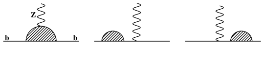
Figure 2: General Feynman diagrams relevant for $t$-mixing corrections to $R_{b}$. The direct vertex correction and the b-quark self-energies sum up to yield a UV finite result.

Before even starting to compute the correction to the left-handed $Z^{o}b\bar{b}$ vertex we can infer some of its properties from gauge invariance. If the external gauge boson was a photon (and not a $Z^{o}$) then the electron self energies and the vertex correction shown in Figure 2 would exactly cancel at zero momentum transfer ($q^{2}=0$) as a consequence of the electromagnetic Ward Identity. With broken gauge symmetry and the external gauge boson being a $Z^{o}$ those terms of the correction that remain unchanged still cancel. Specifically these are the divergencies (i.e. the total correction to $\delta g_{L}^{b}$ is UV finite) and the terms proportional to the coupling of the photon (i.e. the electric charge $Q$ and hence $s_{w}^{2}$). Away from zero momentum transfer the latter no longer holds, the corresponding correction however turns out to be small. In the SM case one obtains (in the limit of a large top mass, $r\gg 1$): [14]

$${\delta g_{L}^{b}}^{\rm SM}\approx{\alpha\over 16\pi s_{w}^{2}}\left[r+\left(3-{s\over 6}(1-2s_{w}^{2})\right)\ln r\right]$$ (7)

where $r=m_{t}^{2}/M_{W}^{2}$, $s=q^{2}/M_{W}^{2}=M_{Z}^{2}/M_{W}^{2}$ and $\alpha$ is the fine structure constant. As stated above the term proportional to $s$ is numerically small.

Turning now to the case of $t$-mixing what has been said above still holds. Specifically, we can neglect terms proportional to $s$, as they turn out to be irrelevant for the precision needed in the present analysis. Also, although the final result is more complicated, the total correction is still UV finite and independent of electric quark charges.

To diagonalize the $T$-$T^{\prime}$ mass matrix we rotate, as before, the left- and right-handed chiralities separately. These rotations modify the neutral current couplings of the top quarks:

$$g_{L,R}^{ij}=\sum_{a=T,T^{\prime}}g_{L,R}^{a}{\cal U}_{L,R}^{ai}{\cal U}_{L,R}^{aj}$$ (8)

where ${\cal U}$ denotes a two-by-two rotation matrix and $i,j=t,t^{\prime}$. Clearly $t$-mixing introduces flavor changing neutral currents that are of relevance in vertex correction diagrams. The mixing also affects the charged current couplings. In the presence of $b$-mixing one then has ${\cal V}_{tb}=c_{L}c_{L}^{B}+s_{L}s_{L}^{B}$ and ${\cal V}_{t^{\prime}b}=s_{L}c_{L}^{b}+c_{L}s_{L}^{B}$. Here the superscript ^B indicates the b-quark mixing angles. Defining $r^{\prime}\equiv m_{t^{\prime}}^{2}/M_{W}^{2}$ the total correction, $\delta g_{L}^{b}$, can be viewed as a dimensionless, lorentz-invariant form factor which depends on $r$,$r^{\prime}$, the weak isospin assignements of the $T^{\prime}$ field and the mixing angles. Defining the ’net’ correction due to $t$-mixing as the difference between the total and the SM top-quark correction, $\delta g_{L}^{b}={\delta g_{L}^{b}}^{\rm total}-{\delta g_{L}^{b}}^{\rm SM}$, one then obtains [1]

$$\delta g_{L}^{b} = {\alpha\over 16\pi s_{w}^{2}}\left\{{\cal V}_{t^{\prime}b}^{2}\left[r^{\prime}-r+3\ln\left({r^{\prime}\over r}\right)\right]\right.$$

$$\qquad+(1-2{I^{\prime}_{3}}_{L}){\cal V}_{tb}{\cal V}_{t^{\prime}b}s_{L}c_{L}\left[-r-r^{\prime}+{2rr^{\prime}\over r^{\prime}-r}\ln\left({r^{\prime}\over r}\right)\right]$$

$$\qquad+2{I^{\prime}_{3}}_{R}{\cal V}_{tb}^{2}s_{R}^{2}\left[-r+{1\over 2}\left(1+{r\over r^{\prime}}\right){rr^{\prime}\over r^{\prime}-r}\ln\left({r^{\prime}\over r}\right)\right.$$

$$\qquad\qquad\qquad\qquad\left.\left.-{3r\over r^{\prime}-r}\ln\left({r^{\prime}\over r}\right)+{3\over 2}\left(1+{r\over r^{\prime}}\right)\right]\right\}$$

which is valid in the limit of heavy quark masses ($r,r^{\prime}\gg 1$). Upon analyzing this result more in detail one finds that even for $m_{t^{\prime}}>m_{t}$ it is possible to choose ${I^{\prime}_{3}}_{L,R}$ and mixing angles such that the correction is negative [1]. So $t$-mixing can indeed increase $R_{b}$. To see how large an increase we can, in principle, get, we choose the most optimal values for the parameters that control Eq. 3: ${\cal V}_{t^{\prime}b}\approx 1$ and $m_{t^{\prime}}\approx 135$ GeV. In this case the first term of Eq. 3 dominates and one obtains, for $m_{t}=180$ GeV, $\delta g_{L}^{b}\approx-0.0021$ which, according to Table 1, is about a third of what is needed.

4 Conclusions

In summary I have argued that in order to explain the current experimental situation it is necessary and sufficient to modify the theoretical prediction of $R_{b}$. Other deviations from the SM can well be viewed as statistical fluctuations. The needed correction to the $Z^{o}b\bar{b}$ coupling is small, the size of a large one-loop effect, if it were left-handed, or large, corresponding to a tree-level effect, if it were right-handed. In the framework of heavy quark mixing we found that $b$-mixing can indeed explain $R_{b}$ - provided one is ’exotic’ enough. Top quark mixing on the other hand can modify the radiative corrections to the $Z^{o}b\bar{b}$ vertex only to the extend of reducing the discrepancy to the data by one third at best.

References

References

- [1] P. Bamert, C.P. Burgess, J. Cline, D. London and E. Nardi, McGill University preprint McGill/96-04, hep-ph/9602438, (1996).
- [2] LEP electroweak working group and the LEP collaborations, CERN preprint CERN-PPE/95-172, (1995); M.D. Hildreth, ”The Current Status of the and ’Puzzle’ ”, talk given at the XXXIst Rencontres de Moriond, (March 1996).
- [3] SLD Collaboration, as presented at CERN by C. Baltay, (June 1995).
-
[4]
CDF Collaboration, F. Abe et.al.,
Phys. Rev. Lett. 74, 2626 (1995);
DO Collaboration, S. Abachi et.al., Phys. Rev. Lett. 74, 2632 (1995). - [5] J. Cline, these proceedings, hep-ph/9606232, (1996).
- [6] C.P. Burgess, S. Godfrey, H. König, D. London and I. Maksymyk, Phys. Rev. D 49, 6115 (1994).
- [7] M.E. Peskin and T. Takeuchi, Phys. Rev. Lett. 65, 964 (1990); Phys. Rev. D 46, 381 (1992); W.J. Marciano and J.L. Rosner, Phys. Rev. Lett. 65, 2963 (1990); D.C. Kennedy and P. Langacker, Phys. Rev. Lett. 65, 2967 (1990); B. Holdom and J. Terning, Phys. Lett. B 247, 88 (1990).
- [8] P. Bamert, McGill University preprint McGill/95-64, hep-ph/9512445, (1995); P. Bamert, C.P. Burgess and I. Maksymyk, Phys. Lett. B 356, 282 (1995).
- [9] B. Holdom, Phys. Lett. B 339, 114 (1994); J. Erler and P. Langacker, Phys. Rev. D 52, 441 (1995); G. Altarelli, R. Barbieri and F. Caravaglios, Phys. Lett. B 349, 145 (1995); M. Shifman, Mod. Phys. Lett. A10, 605 (1995).
- [10] T.J. LeCompte (CDF Collaboration), Fermilab preprint FERMILAB-CONF-96/021-E (1996).
- [11] E. Ma, Phys. Rev. D 53, 2276 (1996).
- [12] C.-H.V. Chang, D. Chang and W.-Y. Keung, National Tsing-Hua University preprint NHCU-HEP-96-1, hep-ph/9601326, (1996).
-
[13]
T. Yoshikawa, Hiroshima University preprint HUPD-9528,
hep-ph/9512251, (1995). - [14] J. Bernabéu, A. Pich and A. Santamaria, Phys. Lett. B 200, 569 (1988); See also: A.A. Akhundov et.al., Nucl. Phys. B 276, 1 (1986); W. Beenakker and W. Hollik, Z. Phys. C 40, 141 (1988); B.W. Lynn and R.G. Stuart, Phys. Lett. B 252, 676 (1990); J. Bernabéu, A. Pich and A. Santamaria, Nucl. Phys. B 363, 326 (1991)