Abstract

In this paper we compute one-loop corrections to masses and couplings in the minimal supersymmetric standard model. We present explicit formulae for the complete corrections and a set of compact approximations which hold over the unified parameter space associated with radiative electroweak symmetry breaking. We illustrate the importance of the corrections and the accuracy of our approximations by scanning over the parameter space. We calculate the supersymmetric one-loop corrections to the $W$-boson mass, the effective weak mixing angle, and the quark and lepton masses, and discuss implications for gauge and Yukawa coupling unification. We also compute the one-loop corrections to the entire superpartner and Higgs-boson mass spectrum. We find significant corrections over much of the parameter space, and illustrate that our approximations are good to ${\cal O}(1\%)$ for many of the superparticle masses.

Work supported by Department of Energy contract DE–AC03–76SF00515 and by the U.S. National Science Foundation, grant NSF-PHY-9404057.

1 Introduction

Most precision measurements of electroweak parameters agree quite well with the predictions of the standard model [1]. These experiments rule out many possibilities for physics beyond the standard model, but they have not touched supersymmetry, which evades precision constraints because it decouples from standard-model physics if the scale of supersymmetry breaking is more than a few hundred GeV. Definitive tests of supersymmetry will probably have to wait for direct searches at future colliders.

Once supersymmetry is discovered, a host of new questions arise. For example, one would like to test the low energy supersymmetric relations between the particle masses and couplings by making precision measurements of the supersymmetric parameters. One would like to measure the supersymmetric masses as accurately as possible to shed light on the origin of supersymmetry breaking. Furthermore, one would also like to know whether weak-scale supersymmetry sheds any light on physics at even higher energies. Indeed, the successful unification of gauge couplings encourages hope that other supersymmetric parameters might unify as well. It is important to measure these parameters precisely at low energies so that they can be extrapolated with confidence to higher energies.

It is in this spirit that we present our calculation of one-loop corrections to the minimal supersymmetric standard model (MSSM). We define the MSSM to be the minimally supersymmetrized standard model, with no right handed neutrinos, and all possible soft-breaking terms. We believe that this minimal model provides an appropriate framework for analyzing the phenomenology of supersymmetry and supersymmetric unification.

We approach our calculation in the standard fashion associated with precision electroweak measurements. We take as inputs the electromagnetic coupling at zero momentum, $\alpha_{\rm em}=1/137.036$, the Fermi constant, $G_{\mu}=1.16639\times 10^{-5}$ GeV^-2, the $Z$-boson pole mass, $M_{Z}=91.188$ GeV, the strong coupling in the $\overline{\rm MS}~{}$ scheme at the scale $M_{Z}$, $\alpha_{s}(M_{Z})=0.118$, as well as the quark and lepton masses, $m_{t}=175$ GeV, $m_{b}=4.9$ GeV, and $m_{\tau}=1.777$ GeV [2].

From these inputs, for any tree-level supersymmetric spectrum, we compute the one-loop $W$-boson pole mass, $M_{W}$, as well as the one-loop values of the effective weak mixing angle, $\sin^{2}\theta^{\rm lept}_{\rm eff}$, and the $\overline{\rm DR}~{}$ [3] weak mixing angle, $\hat{s}^{2}$. We also compute the one-loop corrections to the quark and lepton Yukawa couplings, as well as the masses of all the supersymmetric and Higgs particles.

We work in the $\overline{\rm DR}~{}$ scheme, and take the tree-level masses to be given in terms of the running $\overline{\rm DR}~{}$ parameters. For each (bosonic) particle, we determine the one-loop pole mass,

$$M^{2}\ =\ \hat{M}^{2}(Q)\ -\ {\cal R}e\,\Pi(M^{2})\ ,$$ (1)

where $\hat{M}(Q)$ is the tree-level $\overline{\rm DR}~{}$ mass, evaluated at the $\overline{\rm DR}~{}$ scale $Q$, and $\Pi(p^{2})$ is the one-loop self-energy. (As usual, $\Pi(p^{2})$ depends on $Q$ and on the masses and couplings of the particles in the loop. There is a similar expression for the fermion pole mass.)

In all our computations we include the full self-energies, which contain both logarithmic and finite contributions. The logarithmic corrections can be absorbed by changes in the scale $Q$. Therefore we checked our logarithmic results against the one-loop supersymmetric renormalization group equations. Since we write our results using Passarino-Veltman functions [4], some of our finite terms are automatically correct. As a further check, we verified that our corrections decouple from electroweak observables.

We present our complete calculations in a series of Appendices. These appendices include the full one-loop corrections to the gauge and Yukawa couplings, as well as the complete one-loop corrections to the entire MSSM mass spectrum. While some of these results are not new (the gauge-boson [5, 6], Higgs-boson [6] and gluino [7, 8, 9, 10] self-energies and the gauge-coupling corrections [5, 11] already appear in the literature), we include the full set of corrections in order to provide a complete, self-contained and more useful reference.

In Appendix A we write the tree-level masses in terms of the parameters of the MSSM, and in Appendix B we define the Passarino-Veltman functions that we use to present our one-loop results. In Appendix C we compute the one-loop radiative corrections to the gauge couplings of the MSSM, and in Appendix D we write the one-loop corrections to the masses. Where appropriate, we evaluate the corrections to the mass matrices to account for full one-loop superparticle mixing. This allows for an accurate determination of the masses and mixing through the entire parameter space. Finally, in Appendix E we discuss the radiative corrections to the Higgs boson masses.

The results in the Appendices hold for the MSSM with the most general pattern of (flavor diagonal) soft supersymmetry breaking. The parameter space is huge because of the large number of operators that softly break supersymmetry. Therefore in the body of the paper we illustrate our results in a reduced parameter space, obtained by assuming that the soft breaking parameters unify at some high scale.

The unification assumption is useful because it reduces the size of the parameter space. Moreover, it implies certain mass relations that can be tested once supersymmetry is discovered. In addition, for any set of parameters, it allows us to determine the unification scale thresholds that are necessary to achieve unification. As we will see, the present set of precision measurements is sufficient to begin to constrain the physics at the unification scale.

We implement the unification assumption by solving the two-loop supersymmetric renormalization group equations subject to two-sided boundary conditions. At the weak scale, we assume a supersymmetric spectrum, and for a given value of the ratio of vacuum expectation values, $\tan\beta$, we use our one-loop corrections to extract the $\overline{\rm DR}~{}$ couplings $g_{1},\ g_{2},\ g_{3},\ \lambda_{t},\ \lambda_{b}$, and $\lambda_{\tau}$ at the scale $M_{Z}$. We then use the two-loop $\overline{\rm DR}~{}$ renormalization group equations [12] to run these six parameters to the scale $M_{\rm GUT}$, which we define to be the scale where $g_{1}$ and $g_{2}$ meet.

We require that the soft breaking parameters unify at the scale $M_{\rm GUT}$. Therefore at $M_{\rm GUT}$ we fix a universal scalar mass, $M_{0}$, a universal gaugino mass, $M_{1/2}$, and a universal trilinear scalar coupling, $A_{0}$. We then run all the soft parameters back down to the scale $M^{2}_{\tilde{q}}=M^{2}_{0}+4M^{2}_{1/2}$, where we calculate the supersymmetric spectrum using the full one-loop threshold corrections that we present in this paper. In section 4 we show that this scale is essentially the scale of the squark masses, and that the other scalar masses and the Higgsino mass are correlated with it as well.

We require radiative electroweak symmetry breaking [13], so the CP-odd Higgs mass, $m_{A}$, and the supersymmetric Higgs mass parameter, $|\mu|$, are determined in a full one-loop calculation at the scale $M_{\tilde{q}}$. The sign of $\mu$ is left undetermined. We then iterate the entire procedure to determine a self-consistent solution. Typically, convergence to an accuracy of better than $10^{-4}$ is achieved after four iterations.

Once we have a consistent solution, we use the results of the Appendices to illustrate the one-loop corrections in the reduced parameter space associated with unification. We display results for a randomly chosen sample of 4000 points. Our sample is chosen with a logarithmic measure in the range $1<\tan\beta<60$, $50<M_{1/2}<500$ GeV, $10<M_{0}<1000$ GeV, and with a linear measure in the range $-3M_{\tilde{q}}<A_{0}<3M_{\tilde{q}}.$ (The upper limits on $M_{0}$ and $M_{1/2}$ are chosen so that the squark masses are less than about 1 TeV. While larger squark masses are certainly possible, they reintroduce the fine tunings that supersymmetry is designed to avoid.)

Each of these points corresponds to a (local) minimum of the one-loop scalar potential with the correct electroweak symmetry breaking, and each passes a series of phenomenological constraints: We require the first- and second-generation squark masses to be larger than 220 GeV [14], the gluino mass to be greater than 170 GeV [14], the light Higgs mass to be greater than 60 GeV [2], the slepton masses to be greater than 45 GeV [2], and the chargino masses to be greater than 65 GeV [15]. We also require all the Yukawa couplings to remain perturbative ($\lambda<3.5$) up to the unification scale, and since we assume that $R$-parity is unbroken, we enforce the cosmological requirement that the lightest supersymmetric particle be neutral.

We derive approximations to the radiative corrections that hold with reasonable accuracy over the unified parameter space. Where appropriate, we use scatter plots to illustrate the effectiveness of our approximations. The approximations consist of two parts. First we identify the most important contributions to the one-loop corrections. In most cases these are the loops that involve the strong and/or third generation Yukawa couplings. Then we derive approximations to the loop expressions that hold over the unified parameter space.

In the next section, we discuss the radiative corrections to the effective weak mixing angle, $\sin^{2}\theta^{\rm lept}_{\rm eff}$, and the $W$-boson pole mass, $M_{W}$. We illustrate the magnitudes of the different supersymmetric contributions to these observables. We also discuss the renormalization of the $\overline{\rm DR}~{}$ weak mixing angle, $\hat{s}^{2}$, and comment on the way that it affects the gauge thresholds at the unification scale. In section 3 we examine radiative corrections to the third generation quark and lepton masses. We illustrate the different contributions and present approximations which hold to a few percent. We also examine Yukawa unification and demonstrate the size of the unification-scale Yukawa thresholds. In section 4 we present our results for the radiative corrections to the supersymmetric and Higgs boson particle masses. We find large corrections to the masses of the light superparticles. We compare our results with those of the leading logarithmic approximation and find significant improvements over much of the unified parameter space. These corrections are important for unraveling the underlying supersymmetric structure from the supersymmetric mass spectrum.

2 The weak mixing angle and the $W$-boson mass

Figure 1: Supersymmetric corrections to the effective weak mixing angle, $\sin^{2}\theta^{\rm lept}_{\rm eff}$. Figure (a) shows the corrections from top and bottom squark loops versus the heavy top squark mass $m_{\tilde{t}_{1}}$; (b) shows the neutralino/chargino contribution versus the light chargino mass; (c) shows the slepton correction from all three generations against $m_{\tilde{e}_{L}}$; and (d) shows the complete supersymmetric correction plotted against $m_{{\tilde{\chi}}_{1}^{+}}$.

The calculation of supersymmetric contributions to electroweak observables began in 1984 [5]. Since then, the precise confrontation of electroweak data with theoretical predictions of the MSSM has been an active area of study [16, 11]. Global fits to precision data in the MSSM have been performed by several groups [17]. In this section we display our results for two electroweak observables over the parameter space associated with radiative electroweak symmetry breaking and universal unification-scale boundary conditions. We extract the contributions from the various superpartners, and illustrate the manner in which the different contributions decouple from the low energy observables.

2.1 Effective weak mixing angle

We start by considering the effective weak mixing angle, $s^{2}_{\ell}\equiv\sin^{2}\theta^{\rm lept}_{\rm eff}$. The full one-loop calculation is presented for completeness in Appendix C. The complete result is rather involved; for now we simply say that the calculation follows the outline presented above: We take $\alpha_{\rm em}$, $G_{\mu}$, $M_{Z}$, $\alpha_{s}(M_{Z})$, and the fermion masses as inputs, and compute $s^{2}_{\ell}$ as a function of the supersymmetric masses.

Because we compute the experimental observable $s^{2}_{\ell}$ in terms of other low-energy observables, its one-loop supersymmetric corrections decouple as the supersymmetric masses become larger than $M_{Z}$. From Fig. 1 we see that $s^{2}_{\ell}$ is especially sensitive to light sleptons, and that the sum of the supersymmetric corrections is always negative. We did not plot the Higgs boson and first two generation squark contributions. They are negligible, less than $1\times 10^{-4}$ and $4\times 10^{-5}$ in magnitude, respectively. The corrections to $\mu$-decay and the corrections to the $Z$-$\ell^{+}$-$\ell^{-}$ vertex comprise the nonuniversal corrections to $s_{\ell}^{2}$. The former contributes between $-3$ and $1.5\times 10^{-4}$, the latter between $\pm 1.5\times 10^{-4}$, and their sum is in the range $-4$ to $1\times 10^{-4}$.

With $m_{t}=175$ GeV, we find the standard model value of $s^{2}_{\ell}$ varies between 0.2311 to 0.2315 for Higgs masses in the range $60<m_{h}<130$ GeV. This is subject to an error of $2.5\times 10^{-4}$ from the experimental uncertainty in the electromagnetic coupling evaluated at $M_{Z}$, and to corrections of this same order from higher loop effects [18]. Furthermore, increasing $m_{t}$ by $10$ GeV decreases $s^{2}_{\ell}$ by $3.3\times 10^{-4}.$

These predictions for $s^{2}_{\ell}$ should be compared with the LEP and SLD average [1] of 0.23165 $\pm$ 0.00024. Clearly, the standard model calculation agrees quite well with experiment. The additional contribution from supersymmetry can lower the value of $s_{\ell}^{2}$ slightly below 0.2300, or about 6$\sigma$ below the experimental central value. However, we note that higher-order standard-model corrections, changes in $\alpha_{\rm em}$ and $m_{t}$, and other precision observables should all be systematically taken into account to delineate which regions of parameter space are ruled out by these measurements. We do not attempt such a study here.

The corrections to $s^{2}_{\ell}$ diminish rapidly as the superpartner masses become heavy. For example, if we require $m_{\tilde{\chi}^{+}},\ m_{\tilde{\ell}^{+}},\ m_{h}\ >90$ GeV, we find that $s^{2}_{\ell}$ is shifted by at most $-8\times 10^{-4}$ relative to the standard model value.

Figure 2: Finite corrections to $M_{W}$, in MeV. Figures (a-d) are as in Fig. 1.

2.2 $W$-boson mass

We now turn to our second precision electroweak observable, and compute the one-loop correction to the $W$-boson pole mass, $M_{W}$. In Fig. 2 we illustrate some of the finite corrections. The full finite correction increases the prediction for $M_{W}$ by up to 250 MeV. As with $s_{\ell}^{2}$, the contributions from Higgs bosons and the first two generations of squarks are small, less than 12 and 8 MeV, respectively. The nonuniversal correction is also small, between $-6$ and 15 MeV. For large supersymmetric masses, the prediction reduces to that of the standard model because of decoupling.

For $m_{t}=175$ GeV we find the standard-model value of $M_{W}$ in the range 80.39 to 80.43 GeV, with an error of $\pm$13 MeV from the experimental uncertainty of the electromagnetic coupling. This is subject to additional corrections of the same order from higher-loop effects [18]. If we increase $m_{t}$ by 10 GeV, we find a 65 MeV increase in $M_{W}$.

From our calculations we find that the MSSM value for $M_{W}$ ranges from 80.39 to 80.64 GeV. These numbers can be compared to the current world average, 80.33$\pm$0.15 GeV [2]. With the current experimental error, all of the supersymmetric parameter space lies within 2$\sigma$ of the central value. By the end of the decade, the error on $M_{W}$ is expected to be about 50 MeV. If supersymmetry is not discovered by that time, one might think that a much more exacting test could be performed. However, the limits on the superpartner spectrum will also have increased to the point where the effects on weak-scale observables from virtual supersymmetry will be greatly diminished. For example, imposing the limits $m_{\tilde{\chi}^{+}},\ m_{\tilde{\ell}^{+}},\ m_{h}>90$ GeV, we find that typically $\delta M_{W}<50$ MeV, and at most $\delta M_{W}=100$ MeV.

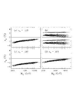
Figure 3: (a) The unification-scale correction, $\varepsilon_{g}$, necessary to obtain $\alpha_{s}(M_{Z})=0.118$, plotted versus $M_{\tilde{q}}$. (b) The maximum and minimum $\varepsilon_{g}$ allowed in minimal SU(5) (top two regions) and missing doublet SU(5) (bottom two regions), against $M_{\tilde{q}}$. (c) Same as (a) with $\alpha_{s}(M_{Z})=0.112$. (d) Same as (a) with $\alpha_{s}(M_{Z})=0.124$.

2.3 Gauge coupling unification

We are now ready to study gauge coupling unification [19]. We start by computing the $\overline{\rm DR}~{}$ electromagnetic coupling constant, $\hat{\alpha}$, and the $\overline{\rm DR}~{}$ weak mixing angle, $\hat{s}^{2}$, as described in Appendix C. The $\overline{\rm DR}~{}$ weak mixing angle is closely related to the effective weak mixing angle, $s^{2}_{\ell}$. The main difference is that $\hat{s}^{2}$ is not an experimental observable, so its radiative corrections involve nondecoupling logarithms of supersymmetric masses. However, once we subtract these logarithms we find finite corrections to $\hat{s}^{2}$ which are quantitatively similar to the corrections to $s^{2}_{\ell}$ shown in Fig. 1.

In the context of gauge coupling unification, the finite corrections to $\hat{s}^{2}$ are very important [20, 21, 22]. They play a significant role in determining the required unification-scale thresholds, which are formally of the same order in perturbation theory. As we will see, precision measurements already limit the size of these thresholds and place constraints on unified models.

We determine the unification thresholds as follows: we calculate the full one-loop corrections to $\hat{\alpha}$ and $\hat{s}^{2}$, and use them to determine the $\overline{\rm DR}~{}$ couplings $g_{1}$ and $g_{2}$. We take $\alpha_{s}(M_{Z})=0.118$ from experiment [2], and apply the supersymmetric threshold corrections to fix the $\overline{\rm DR}~{}$ coupling $g_{3}$ at the scale $M_{Z}$,

$${g_{3}^{2}(M_{Z})\over 4\pi}\ =\ {\alpha_{s}(M_{Z})\over 1-\Delta\alpha_{s}}\ ,$$ (2)

where

$$\Delta\alpha_{s}\ =\ {\alpha_{s}(M_{Z})\over 2\pi}\ \biggl{[}{1\over 2}\ -\ {2\over 3}\ln\left({m_{t}\over M_{Z}}\right)\ -\ 2\ln\left({m_{\tilde{g}}\over M_{Z}}\right)\ -\ {1\over 6}\sum_{\tilde{q}}\sum_{i=1}^{2}\ln\left({m_{\tilde{q}_{i}}\over M_{Z}}\right)\biggr{]}\ .$$ (3)

The sum indexed by $\tilde{q}$ runs over the six squark flavors. The constant in (3) transforms the $\overline{\rm MS}~{}$ coupling $\alpha_{s}(M_{Z})$ into the $\overline{\rm DR}~{}$ coupling $g_{3}$. We also calculate the one-loop $\overline{\rm DR}~{}$ Yukawa couplings $\lambda_{t}(M_{Z}),\ \lambda_{b}(M_{Z})$, and $\lambda_{\tau}(M_{Z})$, as described in the next section.

We then run the six coupled two-loop renormalization group equations [12] up to the unification scale, $M_{\rm GUT}$, which we define to be the point where $g_{1}$ and $g_{2}$ meet. At that scale we define the unification threshold, $\varepsilon_{g}$, to be the discrepancy between $g_{3}$ and the electroweak couplings $g_{1}$ and $g_{2}$,

$$g_{3}(M_{\rm GUT})\ =\ g_{1}(M_{\rm GUT})\,\left(1+\varepsilon_{g}\right)\ .$$ (4)

In Fig. 3(a) we plot the threshold, $\varepsilon_{g}$, versus the squark mass scale, $M_{\tilde{q}}$, which we define to be $M_{\tilde{q}}^{2}\equiv M_{0}^{2}+4M_{1/2}^{2}$. From the figure we see that for $\alpha_{s}(M_{Z})=0.118$, unification requires a negative unification-scale threshold correction of between $-1\%$ and $-3\%$, depending on the weak-scale supersymmetric spectrum. For small $M_{\tilde{q}}$, the finite corrections to the gauge couplings are comparable in size to the logarithmic corrections; they both decrease $\varepsilon_{g}$ at small $M_{\tilde{q}}$.

In order for a unified model to be consistent with gauge coupling unification, it must be able to accommodate values of $\varepsilon_{g}\simeq-2\%$. Different unified models give rise to different unification-scale threshold corrections. In the minimal [23] and missing doublet SU(5) [24] models, $\varepsilon_{g}$ depends only on the triplet Higgs mass [22], the same mass that enters the nucleon decay rate formulae. The maximum and minimum values of $\varepsilon_{g}$ in these two models are shown in Fig. 3(b). The two thin regions correspond to the maximum values of $\varepsilon_{g}$, obtained by setting the triplet Higgs mass to $10^{19}$ GeV. The two larger regions show the minimum values of $\varepsilon_{g}$ in each model. These values are found by setting the triplet Higgs mass as small as possible, consistent with the bounds from nucleon decay [25]. From the figure we see that it is difficult to achieve the necessary thresholds in minimal SU(5), but that missing doublet SU(5) has unification-scale thresholds in the right range.

The unification-scale threshold $\varepsilon_{g}$ necessary for unification is directly correlated with $\alpha_{s}(M_{Z})$. Increasing $\alpha_{s}(M_{Z})$ by 5% increases $\varepsilon_{g}$ by about 1%, as expected from the one-loop relation

$${\delta\alpha_{s}(M_{Z})\over\alpha_{s}(M_{Z})}\ =\ 2\ {\alpha_{s}(M_{Z})\over\alpha_{\rm GUT}}\ \delta\varepsilon_{g}\ .$$ (5)

We illustrate this in Figs. 3(c-d), where we plot $\varepsilon_{g}$ for $\alpha_{s}(M_{Z})=0.112$ and 0.124.

3 Quark and lepton masses

The full set of radiative corrections to the quark and lepton masses is presented in Appendix D. In this section we derive approximations to these formulae, valid for the third generation.

3.1 Top quark mass

The top quark mass provides an important input for radiative electroweak symmetry breaking. It receives strong and electroweak radiative corrections [26, 10]. Our approximation begins by eliminating the small electroweak corrections, setting $g=g^{\prime}=0$ and $\lambda_{t}=\lambda_{b}=0$. We then simplify the resulting expressions by setting $p^{2}=0$ because $m_{t}$ is much smaller than a typical squark or gluino mass.

In this limit, the physical top quark mass is given by

$$m_{t}\ =\ \hat{m}_{t}(Q)\left[\,1+\,{\Delta m_{t}\over m_{t}}\,\right]\ ,$$ (6)

where the one-loop correction receives two important contributions. The first is the well-known gluon correction,

$$\left({\Delta m_{t}\over m_{t}}\right)^{tg}\ = \ {g^{2}_{3}\over 6\pi^{2}}\ \Bigg{[}\,2B_{0}(m_{t},m_{t},0)-B_{1}(m_{t},m_{t},0)\,\Bigg{]}$$ (7)

$$= \ {g^{2}_{3}\over 12\pi^{2}}\ \left[\,3\ln\left({Q^{2}\over m_{t}^{2}}\right)+5\,\right]\ .$$

Note that this contains a logarithmic and a finite piece; the latter gives a 6.6% contribution. The second correction comes from the top squark/gluino loops,

$$\left({\Delta m_{t}\over m_{t}}\right)^{\tilde{t}\tilde{g}}\ = \ -\ {g^{2}_{3}\over 12\pi^{2}}\ \Bigg{\{}\,B_{1}(0,m_{\tilde{g}},m_{\tilde{t}_{1}})+B_{1}(0,m_{\tilde{g}},m_{\tilde{t}_{2}})\,$$ (8)

$$\ -\ \sin(2\theta_{t})\ \left({m_{\tilde{g}}\over m_{t}}\right)\ \Bigg{[}\,B_{0}(0,m_{\tilde{g}},m_{\tilde{t}_{1}})-B_{0}(0,m_{\tilde{g}},m_{\tilde{t}_{2}})\,\Bigg{]}\Bigg{\}}$$

where $\theta_{t}$ is the top-squark mixing angle, and

$$B_{0}(0,m_{1},m_{2})\ =\ -\ \ln\left(M^{2}\over Q^{2}\right)+1+{m^{2}\over m^{2}-M^{2}}\ln\left(M^{2}\over m^{2}\right)\ ,$$ (9)

$$B_{1}(0,m_{1},m_{2})\ =\ {1\over 2}\left[\,-\ \ln\left(M^{2}\over Q^{2}\right)+{1\over 2}+{1\over 1-x}+{\ln x\over(1-x)^{2}}-\theta(1-x)\ln x\,\right]\ ,$$ (10)

with $M=\max(m_{1},m_{2}),$ $m=\min(m_{1},m_{2}),$ and $x=m_{2}^{2}/m_{1}^{2}$. The full $B$ functions are written in Appendix B; the formulae presented here are simplifications that hold when the first argument is zero.

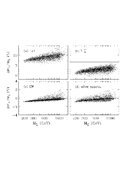
Figure 4: Corrections to the top quark mass, versus $M_{\tilde{q}}$. Figure (a) shows the full one-loop correction. Figure (b) illustrates the correction from the squark/gluino loop; the solid line shows the gluon contribution for comparison. Figure (c) shows the electroweak corrections. In Fig. (d) we plot the difference between the full one-loop result and the approximation given in the text.

In Fig. 4 we show the complete correction to the top quark mass as well as the contributions from the squark/gluino and electroweak loops. The tree-level mass is defined to be $\hat{m}_{t}(m_{t})$. We see that the squark/gluino loop contribution can be as large as the gluon contribution for TeV-scale gluino and squark masses. The electroweak corrections are small because of cancellations. In the figure we also plot the difference between the full correction and our approximation. We see that our approximation is good to typically $\pm 1\%$.

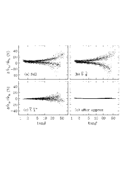
Figure 5: Corrections to the $\overline{\rm DR}~{}$ bottom quark mass $\hat{m}_{b}(M_{Z})$, plotted versus $\tan\beta$. Figure (a) shows the full one-loop correction; (b) illustrates the full correction from the bottom squark/gluino loops; (c) shows the correction from the top squark/chargino loops. Figure (d) plots the difference between the full one-loop result and the approximation given in the text.

3.2 Bottom quark mass

Corrections to the bottom quark mass in the MSSM have received much attention because they can contain significant enhanced supersymmetric contributions [28, 29]. These large contributions play an important role in Yukawa coupling unification. Previous studies have included only the enhanced contributions. In this paper we present our results for the full one-loop correction. Moreover, we systematically develop approximations to the supersymmetric corrections. In this way we can see the importance of the enhanced contributions relative to the full result.

The corrections to the bottom quark mass are found as follows. Because the bottom quark is light, $\alpha_{s}(m_{b})$ is large and we must resum the gluon contribution. We start with the bottom-quark pole mass, $m_{b}$. We find the standard-model $\overline{\rm DR}~{}$ bottom quark mass at the scale $m_{b}$ using the two-loop QCD correction,

$$\hat{m}_{b}(m_{b})^{\rm SM}\ =\ m_{b}\ \left[\,1-\left({\Delta m_{b}\over m_{b}}\right)^{bg}\,\right]\ ,$$ (11)

where [27]

$$\left({\Delta m_{b}\over m_{b}}\right)^{bg}\ =\ {5\over 3}{\alpha_{s}(m_{b})\over\pi}\ +\ 12.4\,\left({\alpha_{s}(m_{b})\over\pi}\right)^{2}\ ,$$ (12)

and $\alpha_{s}(m_{b})$ is the five-flavor three-loop running $\overline{\rm DR}~{}$ coupling. We then evolve this mass to the scale $M_{Z}$ using a numerical solution to the two-loop (plus three-loop ${\cal O}(\alpha_{s}^{3})$) standard-model renormalization group equations [30]. Taking the bottom quark pole mass $m_{b}=4.9$ GeV, and $\alpha_{s}(M_{Z})=0.118$, we find the standard-model $\overline{\rm DR}~{}$ value $\hat{m}_{b}(M_{Z})^{\rm SM}=2.92$ GeV.

The final step is to add the one-loop corrections from massive particles,

$$\hat{m}_{b}(M_{Z})\ =\ \hat{m}_{b}(M_{Z})^{\rm SM}\ \left[\,1-\left({\Delta m_{b}\over m_{b}}\right)^{\rm massive}\,\right]\ .$$ (13)

We approximate these corrections as follows. We ignore the small $W$, $Z$, Higgs, and neutralino contributions. This leaves the squark/gluino and squark/chargino loops,

$$\left({\Delta m_{b}\over m_{b}}\right)^{\rm massive}\ =\ \left({\Delta m_{b}\over m_{b}}\right)^{\tilde{b}\tilde{g}}\ +\ \left({\Delta m_{b}\over m_{b}}\right)^{\tilde{t}\tilde{\chi}^{+}}\ .$$ (14)

We then set $p^{2}=0$. The squark/gluino contribution is again given by (8), with the obvious substitution $t\rightarrow b$. To approximate the squark/chargino contribution, we set $g=g^{\prime}=\lambda_{b}=\lambda_{t}=0$, except for terms that are enhanced by the Higgsino mass parameter $\mu$ or by $\tan\beta$. We simplify our expressions by setting the chargino masses to $M_{2}$ and $\mu$, respectively. In this case the squark/chargino loops give rise to the following terms,

$$\left({\Delta m_{b}\over m_{b}}\right)^{\tilde{t}\tilde{\chi}^{+}}\ =\ {\lambda_{t}^{2}\over 16\pi^{2}}\ \mu\ {A_{t}\tan\beta+\mu\over m_{{\tilde{t}}_{1}}^{2}-m_{{\tilde{t}}_{2}}^{2}}\ \Bigg{[}\,B_{0}(0,\mu,m_{{\tilde{t}}_{1}})-B_{0}(0,\mu,m_{{\tilde{t}}_{2}})\,\Bigg{]}$$

$$+\ {g^{2}\over 16\pi^{2}}\,\Bigg{\{}{\mu M_{2}\tan\beta\over\mu^{2}-M_{2}^{2}}\,\Bigg{[}\,c_{t}^{2}B_{0}(0,M_{2},m_{{\tilde{t}}_{1}})+s_{t}^{2}B_{0}(0,M_{2},m_{{\tilde{t}}_{2}})\Bigg{]}\ +\ (\mu\leftrightarrow M_{2})\ \Bigg{\}}\ ,$$ (15)

where $B_{0}(0,m_{1},m_{2})$ is defined in (9), and $c_{t}\ (s_{t})$ is $\cos\theta_{t}\ (\sin\theta_{t})$.

In Fig. 5 we show the corrections to the $\overline{\rm DR}~{}$ bottom quark mass, $\hat{m}_{b}(M_{Z})$, plotted against $\tan\beta$. Figure 5(a) shows the full one-loop correction, while (b) and (c) illustrate the predominately finite corrections from squark/gluino and squark/chargino loops. At large $\tan\beta$, the top branches in Figs. (a) and (b) correspond to $\mu<0$, while for Fig. (c) the bottom branch corresponds to $\mu<0$. The contributions from Figs. (b) and (c) tend to cancel. Because of the cancellations and large corrections, previous approximations to the bottom quark mass appearing in the literature can be substantially different from the full one-loop result. In Fig. 5(d) we see that the approximation (14) typically agrees with the full one-loop result to within a few percent.

Figure 6: Supersymmetric corrections to the $\overline{\rm DR}~{}$ tau lepton mass $\hat{m}_{\tau}(M_{Z})$, plotted against $\tan\beta$. Figure (a) gives the full one-loop correction; (b) illustrates the difference between the full one-loop result and the approximation given in the text.

3.3 Tau lepton mass

The corrections to the tau lepton mass are of course much smaller than those of the quarks. After resumming the two-loop QED corrections which relate the tau pole mass to the $\overline{\rm DR}~{}$ running mass at $M_{Z}$ [30], we obtain the $\overline{\rm DR}~{}$ mass $\hat{m}_{\tau}(M_{Z})=1.7463$ GeV. We approximate the remaining corrections by setting $p^{2}=0$ and keeping only those terms proportional to $g^{2}$ and enhanced by $\mu$ or $\tan\beta$. The only such terms arise from the chargino loops. They give

$$\left({\Delta m_{\tau}\over m_{\tau}}\right)\ =\ {g^{2}\over 16\pi^{2}}\ {\mu M_{2}\tan\beta\over\mu^{2}-M_{2}^{2}}\ \Bigg{[}\,B_{0}(0,M_{2},m_{\tilde{\nu}_{\tau}})-B_{0}(0,\mu,m_{\tilde{\nu}_{\tau}})\,\Bigg{]}\ ,$$ (16)

where $B_{0}(0,m_{1},m_{2})$ is given in (9). We illustrate the tau corrections in Fig. 6. The full correction ranges from $-10\%$ to $+6\%$, while the approximation is good to within a few $\%$. For large $\tan\beta$, the top branch corresponds to $\mu>0$.

3.4 Yukawa coupling unification

In many supersymmetric unified theories, the $\overline{\rm DR}~{}$ bottom and tau Yukawa couplings are predicted to unify at the scale $M_{\rm GUT}$ [19]. To test this hypothesis, one must first extract the running $\overline{\rm DR}~{}$ Yukawa couplings $\lambda_{b}$ and $\lambda_{\tau}$ from the $\overline{\rm DR}~{}$ bottom and tau masses. Our procedure is as follows. We first use the formulae in Appendix D to find $\overline{\rm DR}~{}$ masses for the bottom and tau. We then use the following relations to find the $\overline{\rm DR}~{}$ Yukawa couplings at the scale $M_{Z}$,

$$\hat{m}_{b}(M_{Z})\ = \ {1\over\sqrt{2}}\,\lambda_{b}(M_{Z})\ v(M_{Z})\cos\beta(M_{Z})$$

$$\hat{m}_{\tau}(M_{Z})\ = \ {1\over\sqrt{2}}\,\lambda_{\tau}(M_{Z})\ v(M_{Z})\cos\beta(M_{Z})\ .$$ (17)

We determine the full one-loop $\overline{\rm DR}~{}$ vev $v(M_{Z})$ from the relation

$$M_{Z}^{2}+{\cal R}e\,\Pi_{ZZ}^{T}(M_{Z}^{2})\ =\ {1\over 4}\biggl{(}g^{2}(M_{Z})+g^{\prime 2}(M_{Z})\biggr{)}v^{2}(M_{Z})$$ (18)

where $g$ and $g^{\prime}$ are the $\overline{\rm DR}~{}$ couplings, and $\Pi_{ZZ}^{T}$ is the transverse $Z$-boson $\overline{\rm DR}~{}$ self-energy. Alternatively, the $\overline{\rm DR}~{}$ vev $v(M_{Z})$ can be taken from the following empirical fit,

$$v(M_{Z})\ =\ \left[\,248.6\ +\ 0.9\,\ln\left({M_{\tilde{q}}\over M_{Z}}\right)\right]\ {\rm GeV}\ .$$ (19)

This expression gives the correct one-loop vev to an accuracy of better than 1%.

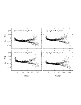
Figure 7: The unification-scale correction, $\varepsilon_{b},$ that is necessary to obtain bottom-tau unification with the given values of $\alpha_{s}(M_{Z})$ and $m_{b}$, plotted versus $\tan\beta$. The bottom quark pole mass is labeled in GeV.

Once we have the $\overline{\rm DR}~{}$ Yukawa couplings at $M_{Z}$, we run them to the unification scale $M_{\rm GUT}$. At that scale we define the unification threshold $\varepsilon_{b}$ to be the discrepancy between the couplings,

$$\lambda_{b}(M_{\rm GUT})\ =\ \lambda_{\tau}(M_{\rm GUT})\,\left(1+\varepsilon_{b}\right)\ .$$ (20)

Of course, the relation between the bottom quark mass and the $\overline{\rm DR}~{}$ Yukawa coupling $\lambda_{b}$ depends strongly on the QCD coupling $\alpha_{s}(M_{Z})$. Therefore we compute $\varepsilon_{b}$ assuming that $\varepsilon_{g}$ has already been chosen so that $\alpha_{s}(M_{Z})$ is some fixed value. Such an analysis is illustrated in Fig. 7(a), where we plot $\varepsilon_{b}$ versus $\tan\beta$ for $\alpha_{s}(M_{Z})=0.118$. From the figure we see the well-known feature that Yukawa unification is possible with $\varepsilon_{b}\simeq 0$ for small $\tan\beta$ ($1.2\,\raise 1.29167pt\hbox{$<$\kern-7.5pt\lower 4.30554pt\hbox{$\sim$}}\,\tan\beta\,\raise 1.29167pt\hbox{$<$\kern-7.5pt\lower 4.30554pt\hbox{$\sim$}}\,1.7$) and large $\tan\beta$ ($15\,\raise 1.29167pt\hbox{$<$\kern-7.5pt\lower 4.30554pt\hbox{$\sim$}}\,\tan\beta\,\raise 1.29167pt\hbox{$<$\kern-7.5pt\lower 4.30554pt\hbox{$\sim$}}\,40$). In the large $\tan\beta$ region we distinguish the two cases, $\mu<0$ and $\mu>0$. For $\mu<0$ we see that $\varepsilon_{b}$ is always far from zero, in the range $-24$ to $-60\%$. For $\mu>0$ we find points which permit bottom-tau unification with $\varepsilon_{b}\simeq 0$. However, they are not generic; $\varepsilon_{b}$ depends sensitively on the parameter space, and varies between $-20$ to $+30\%$.

The discrepancy $\varepsilon_{b}$ is sensitive to the value of $\alpha_{s}(M_{Z})$, as well as the input value for the bottom quark pole mass. We illustrate this in Figs. 7(b-d), for the $(\alpha_{s},\ m_{b})$ values (0.118, 5.2), (0.112, 4.9), and (0.124,  4.9), with $m_{b}$ in GeV. We note that setting $\alpha_{s}(M_{Z})=0.112$ and $m_{b}=5.2$ GeV, we find solutions with $|\varepsilon_{b}|<0.05$ over the whole range $1.3<\tan\beta<30$.

4 Supersymmetric and Higgs boson masses

Figure 8: The masses (a) $m_{\tilde{u}_{L}}$, (b) $m_{\tilde{e}_{L}}$, (c) $|\mu|$, (d) $m_{A}$, (e) $m_{\tilde{\chi}_{1}^{+}}$, and (f) $m_{\tilde{\chi}_{2}^{+}}$, versus $M_{\tilde{q}}$. The lines indicate (a) $M_{\tilde{q}}$, (b) $M_{\tilde{q}}/3$ and $M_{\tilde{q}}$, (c) $M_{\tilde{q}}/2$ and $2M_{\tilde{q}}$, (d) $M_{\tilde{q}}/2$ and $2M_{\tilde{q}}$, (e) $M_{\tilde{q}}/2$, and (f) $M_{\tilde{q}}/2$ and $2M_{\tilde{q}}$. The units for both axes are in GeV.

We will begin our analysis of the supersymmetric spectrum by discussing some of its general features. We will use some of these features when we derive our approximations for the radiative corrections. We will be careful to note when we do, so that one can assess the validity of our approximations in other scenarios.

Figure 9: The ratios (a) $m_{\tilde{\chi}_{1}^{0}}/M_{1/2}$, (b) $m_{\tilde{\chi}_{2}^{0}}/M_{1/2}$, (c) $m_{\tilde{\chi}_{1}^{+}}/M_{1/2}$, and (d) $m_{\tilde{g}}/M_{1/2}$, versus $M_{\tilde{q}}$.

Perhaps the most striking consequence of the universal boundary conditions is the fact that they produce a low energy spectrum which is tightly correlated with the magnitude of the squark mass scale $M^{2}_{\tilde{q}}=M^{2}_{0}+4M^{2}_{1/2}$. In Fig. 8 we show the masses $m_{\tilde{u}_{L}}$, $m_{\tilde{e}_{L}}$, $|\mu|$, $m_{A}$, $m_{\tilde{\chi}_{1}^{+}}$, and $m_{\tilde{\chi}_{2}^{+}}$ versus $M_{\tilde{q}}$. From the figure we see that the squark masses are nearly equal to $M_{\tilde{q}}$, while the other masses are generally within a factor of two or three. The exceptions to this degeneracy include the Higgs boson, $h$, which is always light, and the additional possibilities of a light top squark, a light Higgs sector, and/or light gauginos. Of course, the gaugino masses are nearly proportional to $M_{1/2}$. We find that typically $m_{\tilde{\chi}_{1}^{0}}\simeq 0.4M_{1/2}$, $m_{\tilde{\chi}_{2}^{0}}\simeq m_{\tilde{\chi}_{1}^{+}}\simeq 0.8M_{1/2}$, and $m_{\tilde{g}}\simeq 2.4M_{1/2}$, but there are substantial variations from weak-scale threshold corrections (and from mixing for the charginos/neutralinos). We show the ratios $m_{\tilde{\chi}}/M_{1/2}$ and $m_{\tilde{g}}/M_{1/2}$ versus $M_{\tilde{q}}$ in Fig. 9.

In the rest of this section we discuss the one-loop corrections to the masses of the gluino, the charginos and neutralinos, the squarks, the sleptons, and the Higgs bosons. In the following expressions for the mass corrections we implicitly take the real part of the Passarino-Veltman functions.

4.1 Gluino mass

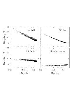
Figure 10: Corrections to the gluino mass versus $m_{\tilde{g}}/M_{\tilde{q}}$. Figure (a) shows the complete one-loop corrections; (b) shows the leading logarithmic corrections; (c) shows the finite corrections; and (d) shows the difference between the full one-loop result and the approximation given in the text.

The gluino mass corrections are perhaps the simplest of all the mass renormalizations. They have previously been studied in Refs. [7, 8, 9, 10]; for completeness we list the corrections in Appendix D. The gluino mass corrections arise from gluon/gluino and quark/squark loops. The corrections can be rather large, so we include them in a way which automatically incorporates the one-loop renormalization group resummation,

$$m_{\tilde{g}}\ =\ M_{3}(Q)\left[\,1-\left({\Delta M_{3}\over M_{3}}\right)^{g\tilde{g}}-\left({\Delta M_{3}\over M_{3}}\right)^{q\tilde{q}}\,\right]^{-1}\ .$$ (21)

The gluon/gluino loop gives

$$\left({\Delta M_{3}\over M_{3}}\right)^{g\tilde{g}}\ = \ {3g^{2}_{3}\over 8\pi^{2}}\ \left[\,2B_{0}(M_{3},M_{3},0)-B_{1}(M_{3},M_{3},0)\,\right]$$ (22)

$$= \ {3g^{2}_{3}\over 16\pi^{2}}\ \left[\,3\ln\left({Q^{2}\over M_{3}^{2}}\right)+5\,\right]\ .$$

The quark/squark loop can be simplified by assuming that all quarks have zero mass, and that all squarks have a common mass, which we take to be $M_{Q_{1}}$, the soft mass of the first generation of left-handed squarks. We find

$$\left({\Delta M_{3}\over M_{3}}\right)^{q\tilde{q}}\ =\ -\ {3g^{2}_{3}\over 4\pi^{2}}\ B_{1}(M_{3},0,M_{Q_{1}})\ .$$ (23)

Here

$$B_{1}(p,0,m)\ =\ -{1\over 2}\ln\left({M^{2}\over Q^{2}}\right)+1-{1\over 2x}\left[\,1+{(x-1)^{2}\over x}\ln|x-1|\,\right]+{1\over 2}\theta(x-1)\ln x\ ,$$ (24)

where $M=\max(p^{2},m^{2})$ and $x=p^{2}/m^{2}$. As usual, the full mass renormalization contains logarithmic and finite contributions.

The gluino mass corrections are shown in Fig. 10. In the figure we define the tree-level gluino mass to be $M_{3}(M_{3})$, and we evaluate the one-loop mass at the scale $Q=M_{\tilde{q}}$. Because we resum the correction, varying the scale from $M_{\tilde{q}}/2$ to $2M_{\tilde{q}}$ changes the one-loop mass by at most $\pm 1\%$.

From the figure we see that the leading logarithmic correction can be as large as 20%, while the finite correction ranges from 3 to 10%. The finite contribution is largest in the region where the logarithm is largest, so the leading logarithm approximation is nowhere good. On the other hand, the approximation we provide typically holds to a few percent. It is off by as much as 6% in the region where the full correction is 30%. In this region we expect the two-loop correction to be of order 6%.

4.2 Neutralino and Chargino Masses

The complete set of corrections to the neutralino and chargino masses [31, 8] is given in Appendix D. In this section we present a set of approximations to these corrections. These approximations are more involved than those discussed above because there are no color corrections that would dominate the results.

Our approximation is as follows. We start by assuming that $|\mu|\,>\,M_{1},M_{2},M_{Z}.$ (We find that $M_{Z}^{2}/\mu^{2}$ and $M_{2}^{2}/\mu^{2}$ are less than 0.53; see Fig. 8). We work with the undiagonalized tree-level (chargino or neutralino) mass matrix, and correct the diagonal entries only, that is, the parameters $M_{1}$, $M_{2}$, and $\mu$. This approximation neglects the corrections to the off-diagonal entries of the mass matrices, which leads to an error of order $(\alpha/4\pi)M^{2}_{Z}/\mu^{2}$ in the masses.

We simplify our expressions by setting all loop masses and external momenta to their diagonal values, i.e. we set $m_{\tilde{\chi}_{1}^{0}}=M_{1}$, etc. We neglect all Yukawa couplings except $\lambda_{t}$ and $\lambda_{b}$. We also ignore the mixings of the charginos and neutralinos in the radiative corrections. This also leads to an error of order $(\alpha/4\pi)M_{Z}^{2}/\mu^{2}$ in our final result.

We further simplify our expressions by setting all quark masses to zero, and by assuming that all squarks are degenerate with mass $M_{Q_{1}}$, and that all sleptons are degenerate as well with mass $M_{L_{1}}$. We also take the Higgs masses to be $m_{h}=M_{Z}$ and $m_{H}=m_{H^{+}}=m_{A}$. This means that we also neglect terms of order $(\alpha/4\pi)M_{Z}^{2}/m_{A}^{2}$.

In this limit, the dominant correction to $M_{1}$ comes from quark/squark, chargino/charged-Higgs and neutralino/neutral-Higgs loops. We find

$$\left({\Delta M_{1}\over M_{1}}\right)\ = \ -{g^{\prime 2}\over 16\pi^{2}}\,\bigg{\{}\,11B_{1}(M_{1},0,M_{Q_{1}})+9B_{1}(M_{1},0,M_{L_{1}})$$ (25)

$$\ +\ {\mu\over M_{1}}\sin(2\beta)\ \bigg{(}\,B_{0}(M_{1},\mu,m_{A})-B_{0}(M_{1},\mu,M_{Z})\,\bigg{)}$$

$$\ +\ B_{1}(M_{1},\mu,m_{A})+B_{1}(M_{1},\mu,M_{Z})\,\bigg{\}}\ .$$

Since $M_{Z},\ M_{1}\ll\mu$, we can simplify this expression by setting $M_{Z}=M_{1}=0$ inside the $B$ functions. This gives

$$\left({\Delta M_{1}\over M_{1}}\right)\ = \ {g^{\prime 2}\over 32\pi^{2}}\,\bigg{\{}\,11\theta_{M_{1}M_{Q_{1}}}+9\theta_{M_{1}M_{L_{1}}}+\theta_{M_{1}\mu M_{Z}}-2B_{1}(0,\mu,m_{A})$$ (26)

$$\ +\ {2\mu\over M_{1}}\sin(2\beta)\ \bigg{(}\,B_{0}(0,\mu,0)\,-\,B_{0}(0,\mu,m_{A})\,\bigg{)}\ -\ {23\over 2}\,\bigg{\}}\ ,$$

where $B_{0}(0,m_{1},m_{2})$ and $B_{1}(0,m_{1},m_{2})$ were defined in (9) and (10), and $\theta_{m_{1}\ldots m_{2}}\equiv\ln(M^{2}/Q^{2})$ with $M^{2}={\rm max}(m_{1}^{2},...,m_{2}^{2})$. The form of the finite corrections depends on the assumed hierarchy in the low-energy spectrum, but the leading logarithms are always correctly given by the $\theta$ terms. We set the first subscript of a $\theta$ term, $m_{1}$, equal to the external momentum. Note that when the renormalization scale equals the external momentum, $Q=m_{1}$, the theta function reduces to the familiar form, $\theta_{m_{1}m_{2}}=\ln(m^{2}_{2}/Q^{2})\,\theta(m^{2}_{2}-Q^{2})$.

The leading logarithmic corrections are easy to read from Eq. (26). Note that the terms proportional to $\sin(2\beta)$ are enhanced by the ratio $\mu/M_{1}$. These finite terms are completely missed in the run-and-match approach because they do not contribute to the beta function.

In a similar way, we approximate the corrections to $M_{2}$ from quark/squark and Higgs loops. They are

$$\left({\Delta M_{2}\over M_{2}}\right)\ = \ -\ {g^{2}\over 16\pi^{2}}\,\bigg{\{}\,9B_{1}(M_{2},0,M_{Q_{1}})+3B_{1}(M_{2},0,M_{L_{1}})$$ (27)

$$\ +\ {\mu\over M_{2}}\sin(2\beta)\ \bigg{(}\,B_{0}(M_{2},\mu,m_{A})-B_{0}(M_{2},\mu,M_{Z})\,\bigg{)}$$

$$\ +\ B_{1}(M_{2},\mu,m_{A})+B_{1}(M_{2},\mu,M_{Z})\,\bigg{\}}\ .$$

Setting $M_{Z}=M_{2}=0$ inside the $B$ functions, we find

$$\left({\Delta M_{2}\over M_{2}}\right)\ = \ {g^{2}\over 32\pi^{2}}\,\bigg{\{}\,9\theta_{M_{2}M_{Q_{1}}}+3\theta_{M_{2}M_{L_{1}}}\ +\ \theta_{M_{2}\mu M_{Z}}-2B_{1}(0,\mu,m_{A})$$ (28)

$$\ +\ {2\mu\over M_{2}}\sin(2\beta)\ \bigg{(}\,B_{0}(0,\mu,0)\,-\,B_{0}(0,\mu,m_{A})\,\bigg{)}\ -\ {15\over 2}\,\bigg{\}}\ .$$

There are additional corrections to $M_{2}$ from gauge boson loops. Because $M_{2}$ enters both the chargino and the neutralino mass matrices, the corrections differ slightly for the two cases. However, to the order of interest, it suffices to use the neutralino result,

$$\left({\Delta M_{2}\over M_{2}}\right)^{\rm gauge}\ =\ {g^{2}\over 4\pi^{2}}\bigg{\{}\,2B_{0}(M_{2},M_{2},M_{W})-B_{1}(M_{2},M_{2},M_{W})\,\bigg{\}}\ .$$ (29)

Because $M_{2}$ is of order $M_{W}$, one must use the full $B$ functions in this expression. Alternatively, one can use the following empirical fit which works to better than 1%,

$$\left({\Delta M_{2}\over M_{2}}\right)^{\rm gauge} = -\ {g^{2}\over 4\pi^{2}}\bigg{\{}\,{3\over 2}\theta_{M_{2}M_{W}}+\theta(M_{W}-M_{2})\left(1.57{M_{2}\over M_{W}}-1.85\right)$$ (30)

$$-\ \theta(M_{2}-M_{W})\,\left[\,0.54\ln\left({M_{2}\over M_{W}}-0.8\right)+1.15\,\right]\,\bigg{\}}\ .$$

The corrections to $\mu$ are obtained in a similar manner. In the limit $g^{\prime 2}\ll g^{2}$, we find

$$\left({\Delta\mu\over\mu}\right)\ = \ -\ {3\over 32\pi^{2}}\bigg{[}\,(\lambda_{b}^{2}+\lambda_{t}^{2})B_{1}(\mu,0,M_{Q_{3}})+\lambda_{t}^{2}B_{1}(\mu,0,M_{U_{3}})+\lambda_{b}^{2}B_{1}(\mu,0,M_{D_{3}})\,\bigg{]}$$

$$\ -\ {3g^{2}\over 64\pi^{2}}\bigg{[}B_{1}(\mu,M_{2},m_{A})+B_{1}(\mu,M_{2},M_{Z})+2B_{1}(\mu,\mu,M_{Z})-4B_{0}(\mu,\mu,M_{Z})\,\bigg{]}\ .$$

As above, we set $M_{Z}=M_{2}=0$ inside the $B$ function, in which case (4.2) reduces to

$$\left({\Delta\mu\over\mu}\right)\ = \ -\ {3\over 32\pi^{2}}\bigg{[}\,(\lambda_{b}^{2}+\lambda_{t}^{2})B_{1}(\mu,0,M_{Q_{3}})+\lambda_{t}^{2}B_{1}(\mu,0,M_{U_{3}})+\lambda_{b}^{2}B_{1}(\mu,0,M_{D_{3}})\,\bigg{]}$$ (32)

$$\ +\ {3g^{2}\over 64\pi^{2}}\bigg{[}{1\over 2}\theta_{\mu M_{2}M_{Z}}\,-\,3\theta_{\mu M_{Z}}\,-\,B_{1}(\mu,0,m_{A})\,+\,4\,\bigg{]}\ .$$

The expression for $B_{1}(p,0,m)$ is given in Eq. (24).

Figure 11: Corrections to the lightest neutralino mass, as in Fig. 10.

In Fig. 11 we show the corrections to the lightest neutralino mass. In Fig. 11(a) we show the full correction in percent, with the tree-level mass defined as the eigenvalue of the mass matrix, where the running parameters $M_{1},\ M_{2},$ and $\mu$ are evaluated at their own scale. (The tree-level mass matrices also contain $\tan\beta$ at $M_{Z}$ and the $W$- and $Z$-boson pole masses.) The one-loop masses have negligible scale dependence.

As usual, the full corrections are made up of logarithmic and finite pieces. The logarithmic corrections are shown in Fig. 11(b) and the finite corrections are shown in Fig. 11(c). Note that the finite corrections can be more than half as large as the logarithmic corrections. Indeed, the finite corrections can be larger than 5% in the small $M_{1}$ region, primarily because of the Higgsino-loop term proportional to $\mu$. In Fig. 11(d) we show the difference between the full one-loop result and our approximation. Here, and in the following two figures, the logarithmic corrections [Fig. 11(b)] include an explicit sum over the soft squark and slepton masses, while the approximations [Fig. 11(d)] use a single soft squark or slepton mass.

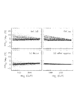
Figure 12: Corrections to the lightest chargino mass, as in Fig. 10.

Figure 12 shows, similarly, the corrections to the lightest chargino mass. Again there is a term proportional to $\mu$ which dominates the finite corrections when $M_{2}$ is small. In this region, the finite corrections can be as large as 10%. In Fig. 12(d) we show that the difference between our approximate correction and the full one-loop mass is less than 2%. These corrections are quantitatively similar to the corrections to the second-lightest neutralino mass.

The corrections to the heavy chargino mass are shown in Fig. 13. These corrections are less than a few percent, as are the corrections for the two heaviest neutralino masses. The logarithmic corrections are in the range 0 to 2.5%, and the finite corrections are in the range 0 to $-3\%$. Figure 13(d) shows that our approximation for the heavy chargino mass generally holds to better than 0.5%. Our approximation also works to typically better than 1% for the two heaviest neutralino masses, but it can be off by nearly 2%.

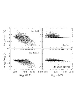
Figure 13: Corrections to the heaviest chargino mass, as in Fig. 10.

4.3 Squark masses

Figure 14: (a) Full one-loop corrections to the first generation squark mass, $m_{\tilde{u}_{L}}$, versus the ratio $m_{\tilde{g}}/m_{\tilde{u}_{L}}$. (b) The difference between the full corrections and the approximation in the text, versus $m_{\tilde{g}}/m_{\tilde{u}_{L}}$. (These are essentially the electroweak corrections.)

The first two generations of squarks receive QCD [32] and electroweak corrections. However, it is a very good approximation to ignore the electroweak graphs, since the dominant corrections come from gluon/squark and gluino/quark loops. Neglecting the quark masses, these corrections are as follows,

$$m_{\tilde{q}}^{2}\ =\ \hat{m}_{\tilde{q}}^{2}(Q)\left[\,1+\left({\Delta m_{\tilde{q}}^{2}\over m_{\tilde{q}}^{2}}\right)\,\right]\ ,$$ (33)

where

$$\left({\Delta m_{\tilde{q}}^{2}\over m_{\tilde{q}}^{2}}\right) = \ {g^{2}_{3}\over 6\pi^{2}}\ \bigg{[}\,2B_{1}(m_{\tilde{q}},m_{\tilde{q}},0)+{A_{0}(m_{\tilde{g}})\over m_{\tilde{q}}^{2}}-(1-x)B_{0}(m_{\tilde{q}},m_{\tilde{g}},0)\,\bigg{]}$$ (34)

$$= \ {g^{2}_{3}\over 6\pi^{2}}\bigg{[}\,1+3x+(x-1)^{2}\ln|x-1|-x^{2}\ln x\ +2x\ln\left({Q^{2}\over m_{\tilde{q}}^{2}}\right)\,\bigg{]}~{},$$

and $x=m_{\tilde{g}}^{2}/m_{\tilde{q}}^{2}$.

For the case of universal boundary conditions the gluino mass is less than or roughly equal to the squark mass, so the correction (34) is essentially finite at $Q=m_{\tilde{q}}$. From Fig. 14 we see that it varies from around 1% for $x\ll 1$ to between 4 and 5% for $x\simeq 1$. We also see that the electroweak corrections are small, less than 0.5%.

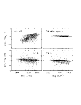
Figure 15: (a) The corrections to the heavy top squark mass versus its mass. (b) The difference between the full one-loop heavy top squark mass and the approximation, Eq. (35). (c) Same as (a), for ${\tilde{b}}_{1}$. (d) Same as (a), for ${\tilde{b}}_{2}$.

The third generation squark masses receive Yukawa corrections on the order of, and opposite in sign to, the QCD corrections. In Fig. 15 we show the full corrections to the third generation heavy squark masses. As usual, the tree-level masses are defined in terms of the gauge-boson and quark pole masses, as well as the soft masses $M_{Q}(M_{Q})$, $M_{U}(M_{U})$, and $M_{D}(M_{D})$. The tree-level mass matrices also contain $\tan\beta(M_{Z})$, $\mu(\mu)$, and $A_{i}({\rm max}(|A_{i}|,M_{Z}))$, where $A_{i}$ denotes the top or bottom $A$-term. (Our convention for the third generation squarks is to associate the subscript 1 with the mostly left-handed squark. Since the light top squark is predominantly right-handed, its mass is denoted $m_{\tilde{t}_{2}}$.)

From Fig. 15 we see that the heavy top squark mass receives corrections in the range $-5$ to 2%, while the bottom squark masses receive corrections mostly in the 0 to 3% range. We note that in none of these cases does the leading logarithm approximation work well: as is the case for all the squarks and sleptons, these corrections are essentially non-logarithmic. (The light top squark mass does receive some substantial logarithmic corrections, but they are generally not larger than the finite corrections.)

We will now present our approximation for the top squark mass matrix. We will derive our approximation for the case of the light top squark, but it also works quite well for the heavy top squark (see Fig. 15(b)). The mass of the light top squark receives potentially large additive corrections proportional to the the strong coupling and the top and bottom Yukawa couplings. We approximate the corrections to $m_{\tilde{t}_{2}}$ by neglecting $g,\ g^{\prime}$ and the Yukawa couplings of the first two generations. We also neglect all quark masses except $m_{t}$, which eliminates all sfermion mixing except for that of the top squarks.

We neglect the mixing of charginos and neutralinos, so the two heavy neutralinos and the heavy chargino all have mass $|\mu|$. We also make the approximations $m_{h}=M_{Z}$ and $m_{H}=m_{H^{+}}=m_{A}$. Finally, we set $p=0$ in the $B$-functions if any of the other arguments is much bigger than $m_{{\tilde{t}}_{2}}$.

This gives the following expressions for the one-loop corrections to the top squark mass matrix,

$${\cal M}_{\tilde{t}}^{2}\ =\ \hat{\cal M}_{\tilde{t}}^{2}(Q)\ +\ \pmatrix{\Delta M^{2}_{LL}&\Delta M^{2}_{LR}\cr\Delta M^{2}_{LR}&\Delta M^{2}_{RR}}\ .$$ (35)

The $\Delta M^{2}$ entries are as follows:

$$\Delta M^{2}_{LL} = \ {g^{2}_{3}\over 6\pi^{2}}\ \bigg{\{}2m_{{\tilde{t}}_{2}}^{2}\left[c_{t}^{2}B_{1}(m_{{\tilde{t}}_{2}},m_{{\tilde{t}}_{1}},0)\ +\ s_{t}^{2}B_{1}(m_{{\tilde{t}}_{2}},m_{{\tilde{t}}_{2}},0)\right]$$ (36)

$$\qquad+\ A_{0}(m_{\tilde{g}})\ +\ A_{0}(m_{t})\ -\ (m_{{\tilde{t}}_{2}}^{2}-m_{\tilde{g}}^{2}-m_{t}^{2})B_{0}(0,m_{\tilde{g}},m_{t})\bigg{\}}$$

$$- {1\over 16\pi^{2}}\bigg{[}\lambda_{t}^{2}s_{t}^{2}A_{0}(m_{{\tilde{t}}_{1}})\ +\ \lambda_{b}^{2}A_{0}(m_{\tilde{b}})$$

$$\qquad-\ 2(\lambda_{t}^{2}+\lambda_{b}^{2})A_{0}(\mu)\ +\ (\lambda_{t}^{2}c_{\beta}^{2}+\lambda_{b}^{2}s_{\beta}^{2})A_{0}(m_{A})\bigg{]}$$

$$- {\lambda_{t}^{2}\over 32\pi^{2}}\bigg{[}\Lambda(\theta_{t},\beta)B_{0}(0,m_{{\tilde{t}}_{1}},m_{A})\ +\ \Lambda(\theta_{t}-{\pi\over 2},\beta)B_{0}(0,0,m_{A})$$

$$\qquad+\ \Lambda(\theta_{t},\beta-{\pi\over 2})B_{0}(0,m_{{\tilde{t}}_{1}},0)\ +\ \Lambda(\theta_{t}-{\pi\over 2},\beta-{\pi\over 2})B_{0}(m_{{\tilde{t}}_{2}},m_{{\tilde{t}}_{2}},m_{Z})\bigg{]}$$

$$- {1\over 16\pi^{2}}\bigg{[}\left(\lambda_{t}^{2}m_{t}^{2}c_{\beta}^{2}\ +\ \lambda_{b}^{2}(\mu c_{\beta}-A_{b}s_{\beta})^{2}\right)B_{0}(0,m_{\tilde{b}},m_{A})$$

$$\qquad+\ \left(\lambda_{t}^{2}m_{t}^{2}s_{\beta}^{2}\ +\ \lambda_{b}^{2}(\mu s_{\beta}+A_{b}c_{\beta})^{2}\right)B_{0}(0,m_{\tilde{b}},0)\bigg{]}$$

$$\Delta M^{2}_{LR} = \ -{g^{2}_{3}\over 6\pi^{2}}c_{t}s_{t}\left[(m_{{\tilde{t}}_{1}}^{2}+m_{{\tilde{t}}_{2}}^{2})B_{0}(m_{{\tilde{t}}_{2}},m_{{\tilde{t}}_{1}},0)\ +\ 2m_{{\tilde{t}}_{2}}^{2}B_{0}(m_{{\tilde{t}}_{2}},m_{{\tilde{t}}_{2}},0)\right]$$ (37)

$$- {g^{2}_{3}\over 3\pi^{2}}m_{t}m_{\tilde{g}}B_{0}(0,m_{t},m_{\tilde{g}})\ -\ {3\lambda_{t}^{2}\over 16\pi^{2}}c_{t}s_{t}A_{0}(m_{{\tilde{t}}_{1}})$$

$$- {\lambda_{t}^{2}\over 32\pi^{2}}\bigg{[}\Omega(\theta_{t},\beta)B_{0}(0,m_{{\tilde{t}}_{1}},m_{A})\ +\ \Omega(-\theta_{t},\beta)B_{0}(0,0,m_{A})$$

$$\qquad+\ \Omega(\theta_{t},{\pi\over 2}+\beta)B_{0}(0,m_{{\tilde{t}}_{1}},0)\ +\ \Omega(-\theta_{t},{\pi\over 2}+\beta)B_{0}(m_{{\tilde{t}}_{2}},m_{{\tilde{t}}_{2}},M_{Z})\bigg{]}$$

$$- {1\over 16\pi^{2}}\bigg{[}-\biggl{(}\lambda_{t}^{2}m_{t}c_{\beta}(\mu s_{\beta}-A_{t}c_{\beta})\ +\ \lambda_{b}^{2}m_{t}s_{\beta}(\mu c_{\beta}-A_{b}s_{\beta})\biggr{)}B_{0}(0,m_{\tilde{b}},m_{A})$$

$$\qquad+\ \lambda_{t}^{2}m_{t}s_{\beta}(\mu c_{\beta}+A_{t}s_{\beta})B_{0}(0,m_{\tilde{b}},0)\bigg{]}$$

$$\Delta M^{2}_{RR} = \ {g^{2}_{3}\over 6\pi^{2}}\ \bigg{\{}2m_{{\tilde{t}}_{2}}^{2}\left[s_{t}^{2}B_{1}(m_{{\tilde{t}}_{2}},m_{{\tilde{t}}_{1}},0)\ +\ c_{t}^{2}B_{1}(m_{{\tilde{t}}_{2}},m_{{\tilde{t}}_{2}},0)\right]$$ (38)

$$\qquad+\ A_{0}(m_{\tilde{g}})\ +\ A_{0}(m_{t})\ -\ (m_{{\tilde{t}}_{2}}^{2}-m_{\tilde{g}}^{2}-m_{t}^{2})B_{0}(0,m_{\tilde{g}},m_{t})\bigg{\}}$$

$$- {\lambda_{t}^{2}\over 16\pi^{2}}\left[c_{t}^{2}A_{0}(m_{{\tilde{t}}_{1}})\ +\ A_{0}(m_{\tilde{b}})\ -\ 4A_{0}(\mu)\ +\ 2c_{\beta}^{2}A_{0}(m_{A})\right]$$

$$- {\lambda_{t}^{2}\over 32\pi^{2}}\bigg{[}\Lambda({\pi\over 2}-\theta_{t},\beta)B_{0}(0,m_{{\tilde{t}}_{1}},m_{A})\ +\ \Lambda(-\theta_{t},\beta)B_{0}(0,0,m_{A})$$

$$\qquad+\ \Lambda({\pi\over 2}-\theta_{t},\beta-{\pi\over 2})B_{0}(0,m_{{\tilde{t}}_{1}},0)\ +\ \Lambda(-\theta_{t},\beta-{\pi\over 2})B_{0}(m_{{\tilde{t}}_{2}},m_{{\tilde{t}}_{2}},m_{Z})\bigg{]}$$

$$- {1\over 16\pi^{2}}\bigg{[}\left(\lambda_{b}^{2}m_{t}^{2}s_{\beta}^{2}+\lambda_{t}^{2}(\mu s_{\beta}-A_{t}c_{\beta})^{2}\right)B_{0}(0,m_{\tilde{b}},m_{A})$$

$$\qquad+\ \lambda_{t}^{2}(\mu c_{\beta}+A_{t}s_{\beta})^{2}B_{0}(0,m_{\tilde{b}},0)\bigg{]}\ .$$

We have defined the two functions

$$\Lambda(\theta_{t},\beta) = \left(2m_{t}\cos\beta\cos\theta_{t}\ -\ (\mu\sin\beta-A_{t}\cos\beta)\sin\theta_{t}\right)^{2}$$ (39)

$$\qquad+\ (\mu\sin\beta-A_{t}\cos\beta)^{2}\sin^{2}\theta_{t}$$

$$\Omega(\theta_{t},\beta) = 2m_{t}^{2}\cos^{2}\beta\sin 2\theta_{t}\ -\ 2m_{t}\cos\beta(\mu\sin\beta-A_{t}\cos\beta)\ .$$ (40)

Note that the running mass matrix $\hat{\cal M}^{2}_{t}(Q)$ in Eq. (35) contains the soft masses $M_{Q}$ and $M_{U}$ (as well as $\mu$, $A_{t}$, etc.) at some common scale, $Q$. In the limit $\lambda_{b}\rightarrow 0$, these expressions are equivalent to the results of Ref. [10], with certain external momenta set to zero.

Figure 16: (a) The full one-loop light top squark mass, versus the tree-level mass (in GeV). On the x-axis we plot sign$(m_{\tilde{t}_{2}}^{2})|m_{\tilde{t}_{2}}^{2}|^{1/2}$, so a negative tree-level mass corresponds to $m_{\tilde{t}_{2}}^{2}<0$. (b) The difference between the full correction and the approximation in the text, versus the one-loop mass. (c) The light top squark mass at one loop, versus $A_{0}/M_{\tilde{q}}$. The solid line corresponds to point (I) in the text, the dashed to point (II). (d) The running and one-loop light top squark mass versus the renormalization scale $Q$, for the choice of parameters (I) (solid) and (II) (dashed) in the text, with $A_{0}/M_{\tilde{q}}=-1.83$ and $-2.2$, respectively. The running mass curves each have points where $m_{\tilde{t}_{2}}^{2}$ becomes negative. In these cases we plot the signed square-root of the mass-squared, as in (a).

These approximations depend on the mass of the light top squark. Normally, one would take it to be the tree-level mass. For the case at hand, however, the choice is more subtle because for very light top squarks, the radiative corrections can be quite large. In fact, the radiative correction can change the top squark mass squared from negative to positive. Therefore we shall take $m_{\tilde{t}_{2}}$ to be the one-loop pole mass, which we find by iteration. (We find the one-loop top squark mixing angle by iteration as well.) We show the light top squark one-loop pole mass versus the tree-level mass in Fig. 16(a), where the tree-level mass is the eigenvalue of the mass matrix which contains the running parameters $M_{U}^{2}$ and $M_{Q}^{2}$ evaluated at their own scale (or $M_{Z}$, whichever is larger; the tree-level mass matrix also contains the top quark and $Z$-boson pole masses, $\tan\beta(M_{Z})$, $\mu(\mu)$, and $A_{t}({\rm max}(|A_{t}|,M_{Z}))$. In Fig. 16(b) we see that our approximation for the light top squark mass holds to within 10 GeV.

With the present unification assumptions, a top squark with mass less than $M_{Z}$ requires that the RR term in the mass matrix be small and that the LR element, proportional to the $A$-term, be large. The light top squark mass results from a cancellation between the diagonal and off-diagonal terms, which requires a fine tuning. We illustrate this in Fig. 16(c), where we plot the light top squark one-loop mass versus $A_{0}/M_{\tilde{q}}$. On the same plot we show the curves corresponding to two choices of parameters, (I) $\tan\beta=20,\ M_{0}=500$ GeV, $M_{1/2}=100$ GeV, and $\mu<0$, and (II) $\tan\beta=5,\ M_{0}=100$ GeV, $M_{1/2}=200$ GeV, and $\mu>0$. Whether at tree-level or one-loop, the parameter $A_{0}$ must be tuned to one part in 75 to obtain a light top squark mass below 50 GeV.

We see from Fig. 16(a) that the light top squark mass-squared can be raised from $-$(100 GeV)² at tree-level to over (100 GeV)² at one loop. For such large corrections, it is important to keep in mind that two-loop effects might be important. The size of these effects can be estimated by the scale dependence of the one-loop mass. In Fig. 16(d) we show the scale dependence at the points (I) and (II), with $A_{0}=-985$ GeV and $A_{0}=-907$ GeV, respectively. We see that as the renormalization scale increases from 100 to 1000 GeV, the running masses vary over a wide range. In contrast, the scale dependence of the one-loop masses is quite mild.

4.4 Slepton masses

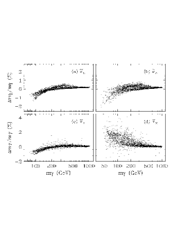
Figure 17: (a) The full set of corrections to the left-handed selectron mass versus its mass. (b) The complete corrections to the electron sneutrino mass versus its mass. The complete corrections to the predominantly (c) left-handed and (d) right-handed tau slepton masses.

Corrections to the SU(2) mass sum rules were studied in Ref. [33]. They suggest that the corrections to the slepton masses are small. We find that the corrections to the left-handed electron or muon slepton masses are typically in the range $\pm 1\%$, as illustrated in Fig. 17(a). The right-handed electron and muon slepton mass corrections are larger, but still less than 1.7%. The sneutrino mass corrections are essentially identical for all three generations. The full correction is typically in the range $\pm 1\%$, and reaches at most $-2.5\%$ at $m_{\tilde{\nu}}\simeq 50$ GeV, as shown in Fig. 17(b). The (predominantly) left- and right-handed tau slepton corrections are similar to the corrections of the first two generation charged slepton masses. However, from Figs. 17(c-d) we see that the scatter plots show less uniformity because of the additional Yukawa coupling corrections. We emphasize that in the corrections to the slepton masses, the leading logarithmic approximation [34] typically gives zero correction. (The mass $m_{\tilde{\tau}_{2}}$ receives some logarithmic corrections. However, the finite corrections are typically of the same order as or larger than the logarithmic corrections.)

4.5 Higgs boson masses

We first discuss the corrections to the heavy Higgs boson masses ($m_{A},\ m_{H},\ m_{H^{+}}$), and then we consider the one-loop light Higgs boson mass. The full one-loop corrections to the Higgs boson masses appear in Ref. [6].

As usual, we parametrize all the Higgs boson masses at tree-level in terms of the CP-odd Higgs boson mass, $m_{A}$, and $\tan\beta$. To compute the one-loop mass $m_{A}$, we first take the soft masses $m_{H_{1}}^{2}(Q)$ and $m_{H_{2}}^{2}(Q)$ as outputs from the renormalization group equations, and apply corrections from the electroweak symmetry breaking conditions to obtain the $\overline{\rm DR}~{}$ running parameters $\hat{m}_{A}^{2}(Q)$ and $\mu^{2}(Q)$ (see Appendix E). We then apply further corrections to obtain the CP-odd Higgs boson pole mass, $m_{A}$, from the running mass, $\hat{m}_{A}(Q)$,

$$m_{A}^{2}\ =\ \hat{m}_{A}^{2}(Q)\ -\ {\cal R}e\,\Pi_{AA}(m_{A}^{2})\ +\ c^{2}_{\beta}{t_{2}\over v_{2}}\ +\ s^{2}_{\beta}{t_{1}\over v_{1}}\ ,$$ (41)

where $t_{1}$ and $t_{2}$ are the tadpole contributions listed in Appendix E. Note that we treat the Higgs mass analogously to the superpartner masses, in that we compare the pole mass with the running mass. However, the Higgs mass is different because the tadpole, or effective potential, corrections must be added to the “tree-level” running mass to obtain the $\overline{\rm DR}~{}$ running mass, $\hat{m}_{A}(Q)$.

The difference between the running mass and the pole mass can be quite substantial; as for the light top squark, the radiative corrections can change a negative mass-squared running mass into a positive mass-squared pole mass. In Fig. 18(a) we show the one-loop pole mass, $m_{A}$, evaluated at $Q=M_{\tilde{q}}$, versus the running mass, $\hat{m}_{A}(m_{A})$.

Figure 18: (a) The one-loop pole mass, $m_{A}$, versus the running mass at the scale $m_{A}$ (the ordinate is the signed square-root of the mass-squared, sign$(\hat{m}_{A}^{2})|\hat{m}_{A}^{2}|^{1/2}$); (b) the corrections to the charged Higgs mass, $m_{H^{+}}$, versus $m_{H^{+}}$.

From Fig. 18(a) we see that there are points in parameter space where the running mass-squared is $-1$ TeV², while the one-loop mass is over 300 GeV. (If one considers the running mass at the scale $M_{Z}$, the largest corrections are even more extreme.) These large corrections arise from terms enhanced by $\tan\beta$. In fact, all of the points in Fig. 18(a) with $\hat{m}_{A}^{2}(m_{A})<0$ occur for $\tan\beta>25$. The $\tan\beta$ enhanced contributions come only from the last term in (41) since $1/v_{1}$ scales like $\tan\beta$ for large $\tan\beta$. Therefore the $\tan\beta$ enhanced corrections are simply

$$m_{A}^{2}\ -\ \hat{m}_{A}^{2}(Q) = {3s_{\beta}^{2}\mu\tan\beta\over 16\pi^{2}}\bigg{\{}\,\lambda_{t}^{2}A_{t}\ B_{0}(0,m_{{\tilde{t}}_{1}},m_{{\tilde{t}}_{2}})\ +\ \lambda_{b}^{2}A_{b}\ B_{0}(0,m_{{\tilde{b}}_{1}},m_{{\tilde{b}}_{2}})$$ (42)

$$\ +\ g^{2}M_{2}\left(1-{M_{2}^{2}\over\mu^{2}}\right)B_{0}(0,\mu,M_{2})\bigg{\}}~{},$$

where $B_{0}(0,m_{1},m_{2})$ is given in (9). These terms account for the large corrections seen in Fig. 18(a).

We parametrize the other heavy Higgs boson masses in terms of the pole mass, $m_{A}$. The corrections to the heavy Higgs boson masses, $m_{H^{+}}$ and $m_{H}$, turn out to be quite small. For example, the corrections to $m_{H^{+}}$ are typically less than 1%, as shown in Fig. 18(b). Corrections to the charged Higgs mass are the subject of Ref. [35].

Figure 19: Figure (a) shows the full one-loop light Higgs mass versus $\tan\beta$. The line indicates the tree-level bound $m_{h}<M_{Z}|\cos 2\beta|$. Figure (b) shows the contribution from the gauge/Higgs/gaugino/Higgsino loops; (c) shows the difference between the full one-loop result and Dabelstein’s approximation; and (d) shows the difference between the full one-loop mass evaluated at the scales $M_{\tilde{q}}$ and $M_{\tilde{q}}/2$.

The corrections to the light Higgs boson mass, $m^{2}_{h}$, have been studied extensively in the literature [36, 6, 37]. Here we show our results for the full one-loop pole mass over the parameter space associated with radiative electroweak symmetry breaking and universal unification-scale boundary conditions. We also show the size of a set of corrections which are often neglected, and the accuracy of Dabelstein’s approximation [37].

In Fig. 19(a) we show the one-loop light Higgs boson mass versus $\tan\beta$, as well as the upper limit at tree level, $m_{h}=M_{Z}|\cos 2\beta|$. The upper limit on the one-loop Higgs mass depends sensitively on the top quark mass, and somewhat less sensitively on the squark masses. In the parameter space we consider the squark masses are less than about 1 TeV. With $m_{t}=175$ GeV, we find $m_{h}<130$ GeV.

In Fig. 19(b) we show the gauge/Higgs/gaugino/Higgsino contribution to the Higgs mass, which is typically $-2$ GeV. In Fig. 19(c) we show the difference between the one-loop result and Dabelstein’s approximation, Eq. (4.9) of Ref. [37], which only includes the top sector. We see that this approximation is typically 2 to 6 GeV larger than the full one-loop mass.

In any pole mass, the scale dependence formally cancels. However, at any given order, there are usually higher-order corrections which do not cancel. For example, when we vary the scale in the Higgs mass calculation, we change the tree-level $\overline{\rm DR}~{}$ mass. To one-loop order, this variation is canceled by the change in the self-energy. However, as the scale varies, the couplings and masses in the self-energies also change. For the case of the Higgs mass, the change in the top quark Yukawa coupling gives rise to a two-loop ${\cal O}(\lambda_{t}^{4})$ scale dependence in our one-loop results. In Fig. 19(d) we show the difference between the full one-loop result evaluated at the scale $M_{\tilde{q}}$ and $M_{\tilde{q}}/2$. We see that the scale dependence is usually small, in the range 0 to $-1$ GeV. The fact that it is negative follows from the dependence of $\tan\beta$ on $Q$, and from the dependence of $\lambda_{t}$ on $\tan\beta$.

5 Conclusions

In this paper we computed one-loop radiative corrections in the minimal supersymmetric standard model. We took as inputs the electromagnetic coupling at zero momentum, $\alpha_{\rm em}$, the Fermi constant, $G_{\mu}$, the $Z$-boson pole mass, $M_{Z}$, the strong coupling in the $\overline{\rm MS}~{}$ scheme at the scale $M_{Z}$, $\alpha_{s}(M_{Z})$, and the quark and lepton masses. From these we computed the $W$-boson mass, $M_{W}$, as well as the one-loop value of the effective weak mixing angle, $\sin^{2}\theta^{\rm lept}_{\rm eff}$, as a function of the supersymmetric parameters.

We studied the size of the corrections in a reduced parameter space associated with the unification of the soft breaking parameters and radiative electroweak symmetry breaking. We found that supersymmetric radiative corrections can reduce $\sin^{2}\theta^{\rm lept}_{\rm eff}$ by as much as $-1.6\times 10^{-3}$ with respect to the standard-model value. Similarly, we found that they can increase $M_{W}$ by as much as 250 MeV. Because of decoupling, the points with the largest deviations are also the points with the lightest superpartners. As direct searches increase the limits on the superparticle masses, the size of the supersymmetric radiative corrections will decrease. Indeed, if superparticles are not discovered at LEP 2, we found that the maximum size of the supersymmetric radiative corrections will be reduced by a factor of two.

The apparent unification of the SU(3), SU(2), and U(1) coupling constants is a major piece of evidence in favor of supersymmetry. At next-to-leading order, the weak- and unification-scale threshold corrections come into play. The weak-scale thresholds decrease the one-loop weak mixing angle. This leads to an increase in the predicted value of the strong coupling, $\alpha_{s}(M_{Z})$. As we have seen, for squark masses less than one TeV, a unification-scale threshold of $-1$ to $-3\%$ is necessary to bring $\alpha_{s}(M_{Z})$ into accord with experiment.

The size of the unification-scale thresholds places an important constraint on unified model building. In any unified model, the unification-scale thresholds can be calculated as a function of the grand unification parameters. One can see whether the model is consistent with a unification-scale threshold of about $-2\%$. In this paper we studied the minimal SU(5) model and the missing doublet SU(5) model. We found that the former was not compatible with gauge coupling unification, while the latter was.

Grand unified theories also predict the unification of certain Yukawa couplings, and in a similar fashion, the mismatch of the Yukawa couplings at the unification scale can be used to constrain unification-scale physics. To this end it is necessary to extract as precisely as possible the $\overline{\rm DR}~{}$ Yukawa couplings from the fermion pole masses. In this paper we presented full one-loop relations between the two, as well as approximations that work at the $\cal O$(1%) level. We studied the substantial (up to 50%) $\tan\beta$-enhanced corrections to the bottom quark mass, as well as the corrections to the top and tau masses, which are of order 5 percent.

Supersymmetry also predicts relations between the masses and couplings of the supersymmetric particles. Indeed, if new particles are discovered at future colliders, it will be necessary to check these relations to see whether the new particles are in fact supersymmetric partners [38]. The radiative corrections to the supersymmetric mass spectrum presented in this paper will be an essential element in these determinations.

The corrections to the supersymmetric mass spectrum will be used in (at least) two ways. First, they will be used to correct the tree-level mass sum rules [33, 39] which test supersymmetry at the weak scale. Second, they will be needed to extract the underlying soft parameters from the physical observables. The soft parameters can then be run to higher scales, to test for unification and possibly to shed light on the origin of the supersymmetry breaking.

The corrections to the supersymmetric masses in the spin-1/2 sector include potentially 30% corrections to the gluino mass, as well as $\cal O$(5%) corrections to the neutralino and chargino masses. In the spin-0 sector, the famous quadratic divergences give rise to large corrections to the scalar masses. These corrections can lift the running mass-squared of the light top squark from $-(100$ GeV$)^{2}$ to (100 GeV)². Even more dramatically, large $\tan\beta$ corrections can lift the mass-squared of the CP-odd Higgs boson from, e.g., $-(1$ TeV)² to (300 GeV)².

Radiative corrections also have an important effect on the mass of the lightest Higgs boson, $h$. In the parameter space we consider, they effectively change the sign of the tree-level bound from $m_{h}<M_{Z}|\cos 2\beta|$ to $m_{h}>M_{Z}|\cos 2\beta|$. We found the light Higgs mass was raised to at most 130 GeV. The corrections to the rest of the scalar masses are smaller. For example, we found 1 to 5% corrections to the first two generation squark masses, and $\cal O$(1%) corrections to the slepton masses.

In the paper we presented approximations to many of the formulae for the supersymmetric mass corrections. These approximations, often good to better than a couple of percent, provide useful substitutes for the full corrections.

Acknowledgements

D.M.P. thanks M. Peskin, T. Rizzo and J. Wells for useful discussions.

Appendix A: Tree-level masses

In this appendix we define the tree-level masses. These tree-level relations also hold for the running $\overline{\rm DR}~{}$ parameters at a common scale, $Q$. For the most part we follow the conventions of Ref. [40].

The up- and down-type quark and charged-lepton masses are related to the Yukawa couplings and the vev’s $v_{1}$ and $v_{2}$ by

$$m_{u}\ =\ {1\over\sqrt{2}}\lambda_{u}v_{2}~{},\qquad\qquad\qquad m_{d}\ =\ {1\over\sqrt{2}}\lambda_{d}v_{1}~{}.$$ (A.1)

The ratio of vev’s $v_{2}/v_{1}$ is denoted $\tan\beta$. The tree-level gauge boson masses are

$$M_{W}^{2}\ =\ {1\over 4}g^{2}\left(v_{1}^{2}+v_{2}^{2}\right)\ ,\qquad\qquad\qquad M_{Z}^{2}\ =\ {1\over 4}\left(g^{\prime 2}+g^{2}\right)\left(v_{1}^{2}+v_{2}^{2}\right)\ ,$$ (A.2)

where $g$ and $g^{\prime}$ are the $SU(2)$ and $U(1)$ gauge couplings.

The Lagrangian contains the neutralino mass matrix as $-{\tilde{\psi}^{0}}{}^{T}{\cal M}_{\tilde{\psi}^{0}}\tilde{\psi}^{0}$ + h.c., where $\tilde{\psi}^{0}=$ $(-i\tilde{b},$ $-i\tilde{w}_{3},$ $\tilde{h}_{1},$ $\tilde{h}_{2})^{T}$ and

$${\cal M}_{\tilde{\psi}^{0}}\ =\ \left(\begin{array}[]{cccc}M_{1}&0&-M_{Z}c_{\beta}s_{W}&M_{Z}s_{\beta}s_{W}\\ 0&M_{2}&M_{Z}c_{\beta}c_{W}&-M_{Z}s_{\beta}c_{W}\\ -M_{Z}c_{\beta}s_{W}&M_{Z}c_{\beta}c_{W}&0&\mu\\ M_{Z}s_{\beta}s_{W}&-M_{Z}s_{\beta}c_{W}&\mu&0\end{array}\right)\ .$$ (A.3)

We use $s$ and $c$ for sine and cosine, so that $s_{\beta}\equiv\sin\beta,\ c_{2\beta}\equiv\cos 2\beta$, etc. $M_{1}$ and $M_{2}$ are the soft supersymmetry-breaking bino and wino gaugino masses, $\mu$ is the supersymmetric Higgsino mass, and $s_{W}\ (c_{W})$ is the sine (cosine) of the weak mixing angle. The neutralino masses are found by acting on the matrix ${\cal M}_{\tilde{\psi}^{0}}$ with a unitary matrix $N$, so that $N^{*}{\cal M}_{\tilde{\psi}^{0}}N^{\dagger}$ is a diagonal matrix which contains the physical neutralino masses, $m_{\tilde{\chi}_{i}^{0}}$. In the usual case that one of the eigenvalues of (A.3) is negative, the matrix $N$ is complex even if the elements of ${\cal M}_{\tilde{\psi}^{0}}$ are real.

The Lagrangian contains the chargino mass matrix as $-{\tilde{\psi}^{-}}{}^{T}{\cal M}_{\tilde{\psi}^{+}}\tilde{\psi}^{+}$ + h.c., where  $\tilde{\psi}^{+}=(-i\tilde{w}^{+},\ \tilde{h}_{2}^{+})^{T},\ \tilde{\psi}^{-}=(-i\tilde{w}^{-},\ \tilde{h}_{1}^{-})^{T}$ and

$${\cal M}_{\tilde{\psi}^{+}}\ =\ \left(\begin{array}[]{cc}M_{2}&\sqrt{2}\,M_{W}s_{\beta}\\ \sqrt{2}\,M_{W}c_{\beta}&-\mu\end{array}\right)\ .$$ (A.4)

The chargino masses are found by acting on the matrix ${\cal M}_{\tilde{\psi}^{+}}$ with a biunitary transformation, so that $U^{*}{\cal M}_{\tilde{\psi}^{+}}V^{\dagger}$ is a diagonal matrix containing the two chargino mass eigenvalues, $m_{\tilde{\chi}_{i}^{+}}$. The matrices $U$ and $V$ are easily found, as they diagonalize, respectively, the matrices ${\cal M}_{\tilde{\psi}^{+}}^{*}{\cal M}_{\tilde{\psi}^{+}}^{\rm T}$ and ${\cal M}_{\tilde{\psi}^{+}}^{\dagger}{\cal M}_{\tilde{\psi}^{+}}$.

At tree level the gluino mass, $m_{\tilde{g}},$ is given by the soft mass, $M_{3}$.

The tree-level squark masses are found by diagonalizing the following mass matrices,

$$\left(\begin{array}[]{cc}M_{Q}^{2}+m_{u}^{2}+g_{u_{L}}M_{Z}^{2}c_{2\beta}&m_{u}\left(A_{u}+\mu\cot\beta\right)\\[5.69054pt] m_{u}\left(A_{u}+\mu\cot\beta\right)&M_{U}^{2}+m_{u}^{2}+g_{u_{R}}M_{Z}^{2}c_{2\beta}\end{array}\right)\ ,$$ (A.5)

$$\left(\begin{array}[]{cc}M_{Q}^{2}+m_{d}^{2}+g_{d_{L}}M_{Z}^{2}c_{2\beta}&m_{d}\left(A_{d}+\mu\tan\beta\right)\\[5.69054pt] m_{d}\left(A_{d}+\mu\tan\beta\right)&M_{D}^{2}+m_{d}^{2}+g_{d_{R}}M_{Z}^{2}c_{2\beta}\end{array}\right)~{}.$$ (A.6)

Here $M_{Q},~{}M_{U},$ and $M_{D}$ are the soft supersymmetry-breaking squark masses, and the $A_{f}$’s are the soft supersymmetry-breaking $A$-terms. The slepton mass matrices are analogous. The soft slepton masses are denoted $M_{L}$ and $M_{E}$. We have defined the weak neutral-current couplings

$$g_{f}\ =\ I^{f}_{3}\ -\ e_{f}s_{W}^{2}~{}.$$ (A.7)

The electric charge, hypercharge, and third component of isospin of the sfermions are

$$\begin{array}[]{cccccccc}&\qquad\tilde{u}_{L}&\qquad\tilde{u}_{R}&\qquad\tilde{d}_{L}&\qquad\tilde{d}_{R}&\qquad\tilde{\nu}&\qquad\tilde{e}_{L}&\qquad\tilde{e}_{R}\\[2.84526pt] \hline\cr\\ e_{f}&\qquad~{}{2\over 3}&\qquad-{2\over 3}&\qquad-{1\over 3}&\qquad~{}{1\over 3}&\qquad~{}0&\qquad-1&\qquad~{}1\\[5.69054pt] Y_{f}&\qquad~{}{1\over 3}&\qquad-{4\over 3}&\qquad~{}{1\over 3}&\qquad{}~{}{2\over 3}&\qquad-1&\qquad-1&\qquad~{}2\\[5.69054pt] I_{3}^{f}&\qquad{}~{}{1\over 2}&\qquad~{}0&\qquad-{1\over 2}&\qquad~{}0&\qquad~{}{1\over 2}&\qquad-{1\over 2}&\qquad~{}0\\[5.69054pt] \hline\cr\\ \end{array}$$ (A.8)

A symbol without an $L$ or $R$ subscript refers to the $L$-field (e.g. $e_{u}=2/3$).

The matrix which diagonalizes a sfermion mass matrix is denoted by

$$\left(\begin{array}[]{cc}c_{f}&s_{f}\\ -s_{f}&c_{f}\end{array}\right)~{},$$ (A.9)

where $c_{f}$ is the cosine of the sfermion mixing angle, $\cos\theta_{f}$, and $s_{f}$ the sine. These angles are given by

$$\tan(2\theta_{u}) = {2m_{u}\left(A_{u}+\mu\cot\beta\right)\over M_{Q}^{2}-M_{U}^{2}+({1\over 2}-2e_{u}s_{W}^{2})M_{Z}^{2}c_{2\beta}}\ ,$$ (A.10)

$$\tan(2\theta_{d}) = {2m_{d}\left(A_{d}+\mu\tan\beta\right)\over M_{Q}^{2}-M_{D}^{2}+(-{1\over 2}-2e_{d}s_{W}^{2})M_{Z}^{2}c_{2\beta}}\ .$$ (A.11)

Since there is no right-handed sneutrino, the slepton mixing angle for $\tilde{\nu}$ satisfies $c_{\nu}=1$, and the sneutrino mass is $m_{\tilde{\nu}}^{2}=M_{L}^{2}+M_{Z}^{2}c_{2\beta}/2$.

Given values for $\tan\beta$ and the CP-odd Higgs-boson mass, $m_{A}$, the other Higgs masses are given, at tree level, by

$$m_{H,h}^{2}\ =\ {1\over 2}\Biggl{(}m_{A}^{2}+M_{Z}^{2}\pm\sqrt{\left(m_{A}^{2}+M_{Z}^{2}\right)^{2}-4m_{A}^{2}M_{Z}^{2}c_{2\beta}^{2}}\Biggr{)}\ ,$$ (A.12)

and

$$m_{H^{+}}^{2}\ =\ m_{A}^{2}\ +\ M_{W}^{2}\ .$$ (A.13)

The CP-even gauge eigenstates $(s_{1},\,s_{2})$ are rotated by the angle $\alpha$ into the mass eigenstates $(H,\,h)$ as follows,

$$\left(\begin{array}[]{c}H\\[5.69054pt] h\end{array}\right)\ =\ \left(\begin{array}[]{cc}c_{\alpha}&s_{\alpha}\\[5.69054pt] -s_{\alpha}&c_{\alpha}\end{array}\right)\left(\begin{array}[]{c}s_{1}\\[5.69054pt] s_{2}\end{array}\right)~{}.$$ (A.14)

At tree level, the angle $\alpha$ is given by

$$\tan 2\alpha\ =\ {m_{A}^{2}+M_{Z}^{2}\over m_{A}^{2}-M_{Z}^{2}}\tan 2\beta~{}.$$ (A.15)

Appendix B: One-loop scalar functions

The following integrals appear at one loop in a self-energy calculation [4]:

$$A_{0}(m) = 16\pi^{2}Q^{4-n}\int{d^{n}q\over i\,(2\pi)^{n}}{1\over q^{2}-m^{2}+i\varepsilon}$$ (B.1)

$$B_{0}(p,m_{1},m_{2}) = 16\pi^{2}Q^{4-n}\int{d^{n}q\over i\,(2\pi)^{n}}{1\over\biggl{[}q^{2}-m^{2}_{1}+i\varepsilon\biggr{]}\biggl{[}(q-p)^{2}-m_{2}^{2}+i\varepsilon\biggr{]}}$$ (B.2)

$$p_{\mu}B_{1}(p,m_{1},m_{2}) = 16\pi^{2}Q^{4-n}\int{d^{n}q\over i\,(2\pi)^{n}}{q_{\mu}\over\biggl{[}q^{2}-m^{2}_{1}+i\varepsilon\biggr{]}\biggl{[}(q-p)^{2}-m_{2}^{2}+i\varepsilon\biggr{]}}$$ (B.3)

$$p_{\mu}p_{\nu}B_{21}(p,m_{1},m_{2}) + g_{\mu\nu}B_{22}(p,m_{1},m_{2})$$

$$= 16\pi^{2}\,Q^{4-n}\,\int{d^{n}q\over i\,(2\pi)^{n}}{q_{\mu}q_{\nu}\over\biggl{[}q^{2}-m^{2}_{1}+i\varepsilon\biggr{]}\biggl{[}(q-p)^{2}-m_{2}^{2}+i\varepsilon\biggr{]}}\ ,$$

where $Q$ is the renormalization scale and we regularize by integrating in $n=4-2\epsilon$ dimensions.

The expression for $A_{0}$ can be integrated to give

$$A_{0}(m)\ =\ m^{2}\left({1\over\hat{\epsilon}}+1-\ln{m^{2}\over Q^{2}}\right)~{},$$ (B.5)

where $1/\hat{\epsilon}=1/\epsilon-\gamma_{E}+\ln 4\pi$.

The function $B_{0}$ can be written in the form

$$B_{0}(p,m_{1},m_{2})\ =\ {1\over\hat{\epsilon}}~{}-~{}\int_{0}^{1}dx\ \ln{(1-x)~{}m_{1}^{2}+x~{}m_{2}^{2}-x(1-x)~{}p^{2}-i\varepsilon\over Q^{2}}\ .$$ (B.6)

It has the analytic expression

$$B_{0}(p,m_{1},m_{2})\ =\ {1\over\hat{\epsilon}}-\ln\left(p^{2}\over Q^{2}\right)-f_{B}(x_{+})-f_{B}(x_{-})~{},$$ (B.7)

where

$$x_{\pm}\ =\ {s\pm\sqrt{s^{2}-4p^{2}(m_{1}^{2}-i\varepsilon)}\over 2p^{2}}~{},\qquad f_{B}(x)\ =\ \ln(1-x)-x\ln(1-x^{-1})-1~{},$$ (B.8)

and $s=p^{2}-m_{2}^{2}+m_{1}^{2}$.

All the other functions can be written in terms of $A_{0}$ and $B_{0}$. For example,

$$B_{1}(p,m_{1},m_{2})\ =\ {1\over 2p^{2}}\biggl{[}A_{0}(m_{2})-A_{0}(m_{1})+(p^{2}+m_{1}^{2}-m_{2}^{2})B_{0}(p,m_{1},m_{2})\biggr{]}~{},$$ (B.9)

and

$$B_{22}(p,m_{1},m_{2}) = {1\over 6}\ \Bigg{\{}\,{1\over 2}\biggl{(}A_{0}(m_{1})+A_{0}(m_{2})\biggr{)}+\left(m_{1}^{2}+m_{2}^{2}-{1\over 2}p^{2}\right)B_{0}(p,m_{1},m_{2})$$ (B.10)

$$+ \ {m_{2}^{2}-m_{1}^{2}\over 2p^{2}}\ \biggl{[}\,A_{0}(m_{2})-A_{0}(m_{1})-(m_{2}^{2}-m_{1}^{2})B_{0}(p,m_{1},m_{2})\,\biggr{]}$$

$$+ \ m_{1}^{2}+m_{2}^{2}-{1\over 3}p^{2}\,\Bigg{\}}~{}.$$

We also define

$$F(p,m_{1},m_{2}) = A_{0}(m_{1})-2A_{0}(m_{2})-(2p^{2}+2m^{2}_{1}-m^{2}_{2})B_{0}(p,m_{1},m_{2})\ ,$$ (B.11)

$$G(p,m_{1},m_{2}) = (p^{2}-m_{1}^{2}-m_{2}^{2})B_{0}(p,m_{1},m_{2})-A_{0}(m_{1})-A_{0}(m_{2})\ ,$$ (B.12)

$$H(p,m_{1},m_{2}) = 4B_{22}(p,m_{1},m_{2})+G(p,m_{1},m_{2})\ ,$$ (B.13)

$$\tilde{B}_{22}(p,m_{1},m_{2}) = B_{22}(p,m_{1},m_{2})-{1\over 4}A_{0}(m_{1})-{1\over 4}A_{0}(m_{2})~{}.$$ (B.14)

The functions $F$ and $G$ arise in scalar self-energies, with either a vector boson and a scalar or fermions in the loop, while $H$ and $\tilde{B}_{22}$ occur in vector-boson self-energies, with either fermions or scalars in the loop.

Appendix C: The gauge couplings

In the remaining appendices we denote $\hat{s}^{2}\equiv\sin^{2}\hat{\theta}_{W}$, where $\hat{\theta}_{W}$ is the $\overline{\rm DR}~{}$ weak mixing angle, and $s^{2}\equiv\sin^{2}\theta_{W}=1-M_{W}^{2}/M_{Z}^{2}$, where $\theta_{W}$ is the “on-shell” weak mixing angle and $M_{W},$ $M_{Z}$ are the gauge-boson pole masses.

The $\overline{\rm DR}~{}$ electromagnetic coupling is given by

$$\hat{\alpha}\ =\ {\alpha_{em}\over 1-\Delta\hat{\alpha}}\ ,\qquad\qquad\alpha_{em}\ =\ {1\over 137.036}\ ,$$ (C.1)

where

$$\Delta\hat{\alpha}\ \ =\ \ 0.0682\pm 0.0007\ -\ {\alpha_{em}\over 2\pi}\Biggl{\{}-7\ln\left(M_{W}\over M_{Z}\right)\ +\ {16\over 9}\ln\left(m_{t}\over M_{Z}\right)\ +\ {1\over 3}\ln\left(m_{H^{+}}\over M_{Z}\right)$$

$$\ +\ {4\over 9}\sum_{u}\sum_{i=1}^{2}\ln\left(m_{\tilde{u}_{i}}\over M_{Z}\right)\ +\ {1\over 9}\sum_{d}\sum_{i=1}^{2}\ln\left(m_{\tilde{d}_{i}}\over M_{Z}\right)\ +\ {1\over 3}\sum_{e}\sum_{i=1}^{2}\ln\left(m_{\tilde{e}_{i}}\over M_{Z}\right)\ +\ {4\over 3}\sum_{i=1}^{2}\ln\left(m_{\tilde{\chi}_{i}^{+}}\over M_{Z}\right)\Biggr{\}}\ ,$$

and $\sum_{u}$ indicates a sum over $u,c,t$, and similarly for $\sum_{d},\ \sum_{e}$. In this expression, the number 0.0682 includes the two-loop QED and QCD corrections given in Ref. [41], as well as the five-flavor contribution $\Delta\alpha^{(5)}_{\rm had}(M_{Z}^{2})=0.0280\pm 0.0007$ of Ref. [42].

The $\overline{\rm DR}~{}$ weak mixing angle is given by [43]

$$\hat{c}^{2}\hat{s}^{2}\ =\ {\pi\hat{\alpha}\over\sqrt{2}\,M_{Z}^{2}\,G_{\mu}\,(1-\Delta\hat{r})}\ ,\qquad\Delta\hat{r}\ =\ \hat{\rho}\ {\Pi_{WW}^{T}(0)\over M_{W}^{2}}\ -\ {\cal R}\!e\ {\Pi_{ZZ}^{T}(M_{Z}^{2})\over M_{Z}^{2}}\ +\ \delta_{\rm VB}\ ,$$ (C.3)

where $\hat{\rho}$ is defined to be $c^{2}/\hat{c}^{2}$, and $\delta_{\rm VB}$ denotes the nonuniversal vertex and box diagram corrections given below. The $W$ and $Z$ gauge-boson self-energies are given in Eqs. (LABEL:piz) and (LABEL:piw). We compute $\hat{\rho}$ via [43]

$$\hat{\rho}\ =\ {1\over 1-\Delta\hat{\rho}}\ ,\qquad\qquad\Delta\hat{\rho}\ =\ {\cal R}\!e\,\Biggl{[}{\Pi_{ZZ}^{T}(M_{Z}^{2})\over\hat{\rho}\,M_{Z}^{2}}\ -\ {\Pi_{WW}^{T}(M_{W}^{2})\over M_{W}^{2}}\Biggr{]}\ .$$ (C.4)

We deduce the leading two-loop standard model corrections to $\Delta\hat{r}$ and $\Delta\hat{\rho}$ from Ref. [41],

$$\Delta\hat{r}\biggr{|}_{\rm 2-loop} = {\hat{\alpha}\over 4\pi\hat{s}^{2}\hat{c}^{2}}{\alpha_{s}\over\pi}\ \Biggl{[}\,2.145{m_{t}^{2}\over M_{Z}^{2}}+0.575\ln\left(m_{t}\over M_{Z}\right)-0.224$$ (C.5)

$$\qquad\qquad-\ 0.144{M_{Z}^{2}\over m_{t}^{2}}\,\Biggr{]}\ -\ {1\over 3}x_{t}^{2}\,\rho^{(2)}\!\!\left(m_{\varphi}\over m_{t}\right)\,(1-\Delta\hat{r})\hat{\rho}\ ,$$

$$\Delta\hat{\rho}\biggr{|}_{\rm 2-loop} = {\hat{\alpha}\over 4\pi\hat{s}^{2}}{\alpha_{s}\over\pi}\ \Biggl{[}\,-2.145{m_{t}^{2}\over M_{W}^{2}}+1.262\ln\left(m_{t}\over M_{Z}\right)-2.24$$ (C.6)

$$\qquad\qquad-\ 0.85{M_{Z}^{2}\over m_{t}^{2}}\,\Biggr{]}\ +\ {1\over 3}x_{t}^{2}\,\rho^{(2)}\!\!\left(m_{\varphi}\over m_{t}\right)\ ,$$

where $x_{t}=3G_{\mu}m_{t}^{2}/8\pi^{2}\sqrt{2}$ and $m_{\varphi}$ is the standard model Higgs-boson mass. For $r\leq 1.9$, $\rho^{(2)}(r)$ is well approximated by [44]

$$\rho^{(2)}(r) = 19-{33\over 2}r+{43\over 12}r^{2}+{7\over 120}r^{3}-\pi\sqrt{r}\left(4-{3\over 2}r+{3\over 32}r^{2}+{1\over 256}r^{3}\right)$$ (C.7)

$$- \pi^{2}(2-2r+{1\over 2}r^{2})-\ln r\left(3r-{1\over 2}r^{2}\right)\ ,$$

while, for $r\geq 1.9$, we use

$$\rho^{(2)}(r) = \ln^{2}r\left({3\over 2}-9r^{-1}-15r^{-2}-48r^{-3}-168r^{-4}-612r^{-5}\right)$$

$$- \ln r\left({27\over 2}+4r^{-1}-{125\over 4}r^{-2}-{558\over 5}r^{-3}-{8307\over 20}r^{-4}-{109321\over 70}r^{-5}\right)$$

$$+ \pi^{2}\left(1-4r^{-1}-5r^{-2}-16r^{-3}-56r^{-4}-204r^{-5}\right)$$

$$+ {49\over 4}+{2\over 3}r^{-1}+{1613\over 48}r^{-2}+{8757\over 100}r^{-3}+{341959\over 1200}r^{-4}+{9737663\over 9800}r^{-5}\ .$$

For the case of the MSSM, we replace the function $\rho^{(2)}(m_{\varphi}/m_{t})$ with

$$\left(\cos\alpha\over\sin\beta\right)^{2}\rho^{(2)}\!\!\left(m_{h}\over m_{t}\right)\ .$$ (C.9)

We have not computed the corresponding $G_{\mu}^{2}m_{t}^{4}$ higher-order contributions from the heavy Higgs bosons, but we know that they must decouple. Using the ansatz

$$\Delta\hat{\rho}\Big{|}_{\rm Heavy\ Higgs}={1\over 3}x_{t}^{2}\biggl{\{}\,\left(\sin\alpha\over\sin\beta\right)^{2}\rho^{(2)}\!\!\left(m_{H}\over m_{t}\right)\ -\left(1\over\tan\beta\right)^{2}\rho^{(2)}\!\!\left(m_{A}\over m_{t}\right)\,\biggr{\}}\ ,$$ (C.10)

we find these contributions are negligible. We do not include them in our results.

The nonuniversal contribution to $\Delta\hat{r}$ is made up of two parts, one from the standard model and the other from supersymmetry,

$$\delta_{\rm VB}\ =\ \delta_{\rm VB}^{\rm SM}\ +\ \delta_{\rm VB}^{\rm SUSY}\ .$$ (C.11)

The standard-model part is given by the well known formula [43]

$$\delta_{\rm VB}^{\rm SM}\ =\ \hat{\rho}\,{\hat{\alpha}\over 4\pi\hat{s}^{2}}\Biggl{\{}6+{\ln c^{2}\over s^{2}}\biggl{[}{7\over 2}-{5\over 2}s^{2}-\hat{s}^{2}\left(5-{3\over 2}{c^{2}\over\hat{c}^{2}}\right)\biggr{]}\Biggr{\}}\ .$$ (C.12)

The supersymmetric part appears in Ref. [5], and more recently in Ref. [11]. We include it here for completeness. It includes box diagram contributions, vertex corrections, and external wave-function renormalizations. We neglect the mixing between different generations of sleptons, and we ignore the left-right slepton mixing in the first two generations, in which case the right-handed sleptons $\tilde{e}_{R},\ \tilde{\mu}_{R}$ do not contribute. We find

$$\delta_{\rm VB}^{\rm SUSY}\ =\ -\ {\hat{s}^{2}\hat{c}^{2}\over 2\pi\hat{\alpha}}M_{Z}^{2}\,{\cal R}e\,a_{1}+\delta v_{e}+\delta v_{\mu}+{1\over 2}\biggl{(}\delta Z_{e}+\delta Z_{\nu_{e}}+\delta Z_{\mu}+\delta Z_{\nu_{\mu}}\biggr{)}\ .$$ (C.13)

The wave-function and vertex corrections are

$$16\pi^{2}~{}\delta Z_{\nu_{e}}\ =\ -\ \sum_{i=1}^{2}\left|b_{\tilde{\chi}_{i}^{+}\nu_{e}\tilde{e}_{L}}\right|^{2}B_{1}(0,m_{\tilde{\chi}^{+}_{i}},m_{\tilde{e}_{L}})-\sum_{j=1}^{4}\left|b_{\tilde{\chi}_{j}^{0}\nu_{e}\tilde{\nu}_{e}}\right|^{2}B_{1}(0,m_{\tilde{\chi}^{0}_{j}},m_{\tilde{\nu}_{e}})~{},$$ (C.14)

$$16\pi^{2}~{}\delta Z_{e}\ =\ -\ \sum_{i=1}^{2}\left|a_{\tilde{\chi}_{i}^{+}e\tilde{\nu}_{e}}\right|^{2}B_{1}(0,m_{\tilde{\chi}^{+}_{i}},m_{\tilde{\nu}_{e}})\ -\ \sum_{j=1}^{4}\left|b_{\tilde{\chi}_{j}^{0}e\tilde{e}_{L}}\right|^{2}B_{1}(0,m_{\tilde{\chi}^{0}_{j}},m_{\tilde{e}_{L}})~{},$$ (C.15)

$$16\pi^{2}~{}\delta v_{e} = \sum_{i=1}^{2}\sum_{j=1}^{4}b_{\tilde{\chi}_{i}^{+}\nu_{e}\tilde{e}_{L}}b^{*}_{\tilde{\chi}_{j}^{0}e\tilde{e}_{L}}\ \Biggl{\{}-\ {\sqrt{2}\over g}a_{\tilde{\chi}_{j}^{0}\tilde{\chi}_{i}^{+}W}m_{\tilde{\chi}_{i}^{+}}m_{\tilde{\chi}_{j}^{0}}\,C_{0}(m_{\tilde{e}_{L}},m_{\tilde{\chi}_{i}^{+}},m_{\tilde{\chi}_{j}^{0}})$$ (C.16)

$$\qquad\qquad+\ {1\over\sqrt{2}g}b_{\tilde{\chi}_{j}^{0}\tilde{\chi}_{i}^{+}W}\ \biggl{[}\,B_{0}(0,m_{\tilde{\chi}_{i}^{+}},m_{\tilde{\chi}_{j}^{0}})+m_{\tilde{e}_{L}}^{2}\,C_{0}(m_{\tilde{e}_{L}},m_{\tilde{\chi}_{i}^{+}},m_{\tilde{\chi}_{j}^{0}})-{1\over 2}\,\biggr{]}\Biggr{\}}$$

$$- \sum_{i=1}^{2}\sum_{j=1}^{4}a_{\tilde{\chi}_{i}^{+}e\tilde{\nu}_{e}}b_{\tilde{\chi}_{j}^{0}\nu_{e}\tilde{\nu}_{e}}\ \Biggl{\{}-\ {\sqrt{2}\over g}b_{\tilde{\chi}_{j}^{0}\tilde{\chi}_{i}^{+}W}m_{\tilde{\chi}_{i}^{+}}m_{\tilde{\chi}_{j}^{0}}\,C_{0}(m_{\tilde{\nu}_{e}},m_{\tilde{\chi}_{i}^{+}},m_{\tilde{\chi}_{j}^{0}})$$

$$\qquad\qquad+\ {1\over\sqrt{2}g}a_{\tilde{\chi}_{j}^{0}\tilde{\chi}_{i}^{+}W}\ \biggl{[}\,B_{0}(0,m_{\tilde{\chi}_{i}^{+}},m_{\tilde{\chi}_{j}^{0}})+m_{\tilde{\nu}_{e}}^{2}\,C_{0}(m_{\tilde{\nu}_{e}},m_{\tilde{\chi}_{i}^{+}},m_{\tilde{\chi}_{j}^{0}})-{1\over 2}\,\biggr{]}\Biggr{\}}$$

$$+ {1\over 2}\sum_{j=1}^{4}b_{\tilde{\chi}_{j}^{0}e\tilde{e}_{L}}^{*}b_{\tilde{\chi}_{j}^{0}\nu_{e}\tilde{\nu}_{e}}\ \biggl{[}\,B_{0}(0,m_{\tilde{e}_{L}},m_{\tilde{\nu}_{e}})+m_{\tilde{\chi}_{j}^{0}}^{2}\,C_{0}(m_{\tilde{\chi}_{j}^{0}},m_{\tilde{e}_{L}},m_{\tilde{\nu}_{e}})+{1\over 2}\,\biggr{]}~{}.$$

The corrections $\delta Z_{\nu_{\mu}},\ \delta Z_{\mu}$, and $\delta v_{\mu}$ are obtained from these expressions by replacing $e\rightarrow\mu$. The $\tilde{\chi}$-fermion-sfermion couplings $a_{\tilde{\chi}_{i}f\tilde{f}_{j}}$ and $b_{\tilde{\chi}_{i}f\tilde{f}_{j}}$ are listed in Eqs. (5–D.22), while the chargino-neutralino-$W$ couplings $a_{\tilde{\chi}_{i}^{0}\tilde{\chi}_{j}^{+}W}$ and $b_{\tilde{\chi}_{i}^{0}\tilde{\chi}_{j}^{+}W}$ are defined in Eqs. (D.12–D.13). In these expressions, the $B_{0}$, $B_{1}$, and $C_{0}$ functions are evaluated at zero momentum,

$$B_{0}(0,m_{1},m_{2})\ =\ {1\over\hat{\epsilon}}+1+\ln\left(Q^{2}\over m_{2}^{2}\right)+{m_{1}^{2}\over m_{1}^{2}-m_{2}^{2}}\ln\left(m_{2}^{2}\over m_{1}^{2}\right)~{},$$ (C.17)

$$B_{1}(0,m_{1},m_{2})\ =\ {1\over 2}\biggl{[}{1\over\hat{\epsilon}}+1+\ln\left(Q^{2}\over m_{2}^{2}\right)+\left({m_{1}^{2}\over m_{1}^{2}-m_{2}^{2}}\right)^{2}\ln\left({m_{2}^{2}\over m_{1}^{2}}\right)+{1\over 2}\left({m_{1}^{2}+m_{2}^{2}\over m_{1}^{2}-m_{2}^{2}}\right)\biggr{]}~{},$$ (C.18)

$$C_{0}(m_{1},m_{2},m_{3})\ =\ {1\over m_{2}^{2}-m_{3}^{2}}\biggl{[}{m_{2}^{2}\over m_{1}^{2}-m_{2}^{2}}\ln\left(m_{2}^{2}\over m_{1}^{2}\right)-{m_{3}^{2}\over m_{1}^{2}-m_{3}^{2}}\ln\left(m_{3}^{2}\over m_{1}^{2}\right)\biggr{]}\ ,$$ (C.19)

where $Q$ is the renormalization scale.

The box diagram contributions are

$$16\pi^{2}~{}a_{1} = {1\over 2}\sum_{i=1}^{2}\sum_{j=1}^{4}a_{\tilde{\chi}_{i}^{+}\mu\tilde{\nu}_{\mu}}b^{*}_{\tilde{\chi}_{i}^{+}\nu_{e}\tilde{e}_{L}}b_{\tilde{\chi}_{j}^{0}\nu_{\mu}\tilde{\nu}_{\mu}}b_{\tilde{\chi}_{j}^{0}e\tilde{e}_{L}}\,m_{\tilde{\chi}_{i}^{+}}\,m_{\tilde{\chi}_{j}^{0}}\,D_{0}(m_{\tilde{e}_{L}},m_{\tilde{\nu}_{\mu}},m_{\tilde{\chi}_{i}^{+}},m_{\tilde{\chi}_{j}^{0}})$$

$$+ {1\over 2}\sum_{i=1}^{2}\sum_{j=1}^{4}a^{*}_{\tilde{\chi}_{i}^{+}e\tilde{\nu}_{e}}b_{\tilde{\chi}_{i}^{+}\nu_{\mu}\tilde{\mu}_{L}}b^{*}_{\tilde{\chi}_{j}^{0}\nu_{e}\tilde{\nu}_{e}}b^{*}_{\tilde{\chi}_{j}^{0}\mu\tilde{\mu}_{L}}\,m_{\tilde{\chi}_{i}^{+}}\,m_{\tilde{\chi}_{j}^{0}}\,D_{0}(m_{\tilde{\mu}_{L}},m_{\tilde{\nu}_{e}},m_{\tilde{\chi}_{i}^{+}},m_{\tilde{\chi}_{j}^{0}})$$

$$+ \sum_{i=1}^{2}\sum_{j=1}^{4}b_{\tilde{\chi}_{i}^{+}\nu_{\mu}\tilde{\mu}_{L}}b^{*}_{\tilde{\chi}_{i}^{+}\nu_{e}\tilde{e}_{L}}b^{*}_{\tilde{\chi}_{j}^{0}\mu\tilde{\mu}_{L}}b_{\tilde{\chi}_{j}^{0}e\tilde{e}_{L}}\,D_{27}(m_{\tilde{\mu}_{L}},m_{\tilde{e}_{L}},m_{\tilde{\chi}_{i}^{+}},m_{\tilde{\chi}_{j}^{0}})$$

$$+ \sum_{i=1}^{2}\sum_{j=1}^{4}a^{*}_{\tilde{\chi}_{i}^{+}\mu\tilde{\nu}_{\mu}}a_{\tilde{\chi}_{i}^{+}e\tilde{\nu}_{e}}b_{\tilde{\chi}_{j}^{0}\nu_{\mu}\tilde{\nu}_{\mu}}b^{*}_{\tilde{\chi}_{j}^{0}\nu_{e}\tilde{\nu}_{e}}\,D_{27}(m_{\tilde{\nu}_{\mu}},m_{\tilde{\nu}_{e}},m_{\tilde{\chi}_{i}^{+}},m_{\tilde{\chi}_{j}^{0}})~{},$$

where the functions $D_{0}$ and $D_{27}$ are

$$D_{0}(m_{1},m_{2},m_{3},m_{4})\ =\ {1\over m_{1}^{2}-m_{2}^{2}}\ \biggl{[}\,C_{0}(m_{1},m_{3},m_{4})-C_{0}(m_{2},m_{3},m_{4})\,\biggr{]}\ ,$$ (C.21)

$$D_{27}(m_{1},m_{2},m_{3},m_{4})\ =\ {1\over 4(m_{1}^{2}-m_{2}^{2})}\ \biggl{[}\,m_{1}^{2}\,C_{0}(m_{1},m_{3},m_{4})-m_{2}^{2}\,C_{0}(m_{2},m_{3},m_{4})\,\biggr{]}\ .$$ (C.22)

We checked our box diagram calculation against Refs. [5, 11], and we checked our formulas for $\delta Z$ and $\delta v$ with those of Ref. [11]. Here (there) the formulas are written in terms of the couplings corresponding to vertices with incoming (outgoing) charginos and neutralinos. To compare we must make the transformation $a_{\tilde{\chi}f\tilde{f}}\leftrightarrow b^{*}_{\tilde{\chi}f\tilde{f}}$, except for couplings involving the chargino and down-type fermions, which remain unchanged. Also, their $\tilde{\chi}^{+}\tilde{\chi}^{0}W$ coupling differs from ours by a sign.

The effective weak mixing angle is given in terms of the $\overline{\rm DR}~{}$ weak mixing angle, $\hat{s}^{2}$, via

$$\sin^{2}\theta_{\rm eff}^{\rm lept}\ =\ \hat{s}^{2}\,{\cal R}e\,\hat{k}_{\ell}$$ (C.23)

where [45]

$$\hat{k}_{\ell}\ =\ 1\ +\ {\hat{c}\over\hat{s}}{\Pi_{Z\gamma}(M_{Z}^{2})-\Pi_{Z\gamma}(0)\over M_{Z}^{2}}\ +\ {\hat{\alpha}\hat{c}^{2}\over\pi\hat{s}^{2}}\ln c^{2}\ -\ {\hat{\alpha}\over 4\pi\hat{s}^{2}}V_{\ell}(M_{Z}^{2})\ ,$$ (C.24)

with

$$V_{\ell}(M_{Z}^{2})\ =\ {1\over 2}f\left({1\over c^{2}}\right)\ +\ 4\hat{c}^{2}g\left({1\over c^{2}}\right)\ -\ {1-6\hat{s}^{2}+8\hat{s}^{4}\over 4\hat{c}^{2}}\,f(1)$$ (C.25)

and

$${\cal R}e\,f(x) = {2\over x}+{7\over 2}-\left(3+{2\over x}\right)\ln x+\left(1+{1\over x}\right)^{2}\biggl{[}\,2{\rm Li}_{2}\left({1\over 1+x}\right)-{\pi^{2}\over 3}+\ln^{2}(1+x)\,\biggr{]}~{},$$

$$g(x) = \left({1\over x}+{1\over 2}\right)\left({\tan^{-1}y\over y}-1\right)+{9\over 8}+{1\over 2x}-\left(1+{1\over 2x}\right){4\over x}\left(\tan^{-1}y\right)^{2}~{}.$$ (C.26)

Here $y\equiv\sqrt{x/(4-x)}$, Li₂ is the Spence function, and $\Pi_{Z\gamma}$ is listed in Eq. (D.15). We do not include here the nonuniversal $Z$-vertex supersymmetric contribution to $\sin^{2}\theta_{\rm eff}^{\rm lept}$. The largest contributions can be obtained from Ref. [46].

Appendix D: One-loop self-energies

In this appendix we list all the relevant self-energy functions which allow us to determine the one-loop fermion, gauge-boson, and superpartner masses. We explicitly include all of the necessary couplings. We perform our calculations in the ’t Hooft-Feynman gauge, in which the Goldstone bosons and the ghosts have the same masses as the corresponding gauge-bosons. The gauge couplings $g^{\prime},\ g,$ and $g_{3}$, and the Yukawa couplings $\lambda_{f}$ are all $\overline{\rm DR}~{}$ couplings. The neutralino mixing matrix $N$, the chargino mixing matrices $U$ and $V$, the Higgs mixing angles $\alpha$ and $\beta$, and the sfermion mixing angles $\theta_{f}$ are described in Appendix A, as are the normalizations of the Yukawa couplings $\lambda_{f}$. The self-energies are given in terms of the Passarino-Veltman functions $A_{0},\ B_{0},\ B_{1},\ F,\ G,\ H$, and $\tilde{B}_{22}$ listed in Appendix B, Eqs. (B.5–B.14).

To streamline notation we do not write explicitly the external momentum dependence of these functions, e.g., we write $B_{0}(p,m_{1},m_{2})$ as $B_{0}(m_{1},m_{2})$. Throughout this appendix we write $s$ for $\sin$, $c$ for $\cos$ and $t$ for $\tan$, so that $s_{\beta}\equiv\sin\beta$, $c_{2\theta_{t}}\equiv\cos 2\theta_{t}$, etc., and for the sfermion mixing angles, $c_{u}\equiv\cos\theta_{u}$, etc. Sub- or superscripts $f$ denote a quark or lepton, and $q$ denotes a quark. Inside a summation $\sum_{f_{u}}$, the subscript or superscript $u$ denotes all up-type (s)fermions, $u,c,t,\nu_{e},\nu_{\mu},\nu_{\tau}$, and similarly inside a summation $\sum_{f_{d}}$, the script $d$ denotes all down-type (s)fermions, $d,s,b,e,\mu,$ and $\tau$. The sum $\sum_{f_{u}/f_{d}}$ denotes a summation over (s)quark and (s)lepton doublets, and the sum $\Sigma_{q}$ denotes a sum over (s)quarks. Some terms are zero, for example $\lambda_{\nu}=0$, and terms involving the right-handed sneutrino are absent.

In the self-energies listed below the $1/\hat{\epsilon}$ poles are canceled by counterterms which relate the bare mass to the running mass. So, in the following $\overline{\rm DR}~{}$ self-energies we implicitly subtract the $1/\hat{\epsilon}$ poles.

$Z$ and $W$ bosons

The full one-loop MSSM gauge-boson self-energies appear in Ref. [5] and subsequently in Ref. [6]. The supersymmetric contributions are listed in Refs. [47, 21, 37].

The self-energies of the gauge-bosons can be separated into transverse and longitudinal pieces, e.g.

$$\Pi^{\mu\nu}_{ZZ}(p^{2})\ =\ \Pi_{ZZ}^{T}(p^{2})\biggl{[}g^{\mu\nu}-{p^{\mu}p^{\nu}\over p^{2}}\biggr{]}\ +\ \Pi_{ZZ}^{L}(p^{2})\,{p^{\mu}p^{\nu}\over p^{2}}\ .$$ (D.1)

The physical gauge-boson masses are the poles of the corresponding propagators, which involve only the transverse part of the gauge-boson self-energy,

$$M_{Z}^{2}\ =\ \hat{M}_{Z}^{2}(Q)\ -\ {\cal R}e\,\Pi^{T}_{ZZ}(M_{Z}^{2})~{},$$ (D.2)

$$M_{W}^{2}\ =\ \hat{M}_{W}^{2}(Q)\ -\ {\cal R}e\,\Pi^{T}_{WW}(M_{W}^{2})~{}.$$ (D.3)

Here $\hat{M}_{Z}(Q)$ and $\hat{M}_{W}(Q)$ denote the $\overline{\rm DR}~{}$ running masses which are related to the $\overline{\rm DR}~{}$ gauge couplings and vev’s, as in Eq. (A.2). The gauge-boson self-energies are evaluated at the renormalization scale $Q$.

The transverse part of the $Z$-boson self-energy is

$$\qquad 16\pi^{2}\,{\hat{c}^{2}\over g^{2}}\,\Pi^{T}_{ZZ}(p^{2}) = -\ s^{2}_{\alpha\beta}\biggl{[}\tilde{B}_{22}(m_{A},m_{H})+\tilde{B}_{22}(M_{Z},m_{h})-M^{2}_{Z}B_{0}(M_{Z},m_{h})\,\biggr{]}$$

$$- c^{2}_{\alpha\beta}\biggl{[}\tilde{B}_{22}(M_{Z},m_{H})+\tilde{B}_{22}(m_{A},m_{h})-M^{2}_{Z}B_{0}(M_{Z},m_{H})\,\biggr{]}$$

$$- 2\hat{c}^{4}\biggl{(}2p^{2}+M_{W}^{2}-M^{2}_{Z}{\hat{s}^{4}\over\hat{c}^{2}}\biggr{)}B_{0}(M_{W},M_{W})$$

$$- (8\hat{c}^{4}+c^{2}_{2\hat{\theta}_{W}})\tilde{B}_{22}(M_{W},M_{W})\ -\ c^{2}_{2\hat{\theta}_{W}}\tilde{B}_{22}(m_{H^{+}},m_{H^{+}})$$

$$- \sum_{f}\sum_{i,j=1}^{2}4N_{c}^{f}v_{fij}^{2}\tilde{B}_{22}(m_{\tilde{f}_{i}},m_{\tilde{f}_{j}})$$

$$+ \sum_{f}N_{c}^{f}\Biggl{\{}\biggl{(}g_{f_{L}}^{2}+g_{f_{R}}^{2}\biggr{)}H(m_{f},m_{f})\ -\ 4g_{f_{L}}g_{f_{R}}m_{f}^{2}B_{0}(m_{f},m_{f})\Biggr{\}}$$

$$+ {\hat{c}^{2}\over 2g^{2}}\sum_{i,j=1}^{4}\Biggl{\{}f_{ijZ}^{0}H(m_{\tilde{\chi}^{0}_{i}},m_{\tilde{\chi}^{0}_{j}})\ +\ 2\,g_{ijZ}^{0}\,m_{\tilde{\chi}^{0}_{i}}m_{\tilde{\chi}^{0}_{j}}B_{0}(m_{\tilde{\chi}^{0}_{i}},m_{\tilde{\chi}_{j}^{0}})\Biggr{\}}$$

$$+ {\hat{c}^{2}\over g^{2}}\sum_{i,j=1}^{2}\Biggl{\{}f^{+}_{ijZ}H(m_{\tilde{\chi}_{i}^{+}},m_{\tilde{\chi}^{+}_{j}})\ +\ 2\,g^{+}_{ijZ}\,m_{\tilde{\chi}^{+}_{i}}m_{\tilde{\chi}^{+}_{j}}B_{0}(m_{\tilde{\chi}_{i}^{+}},m_{\tilde{\chi}^{+}_{j}})\Biggr{\}}~{},$$

where the summation $\sum_{f}$ is over all quarks and leptons, and the color factor $N_{c}^{f}$ is 3 for (s)quarks and 1 for (s)leptons. The notation $s_{\alpha\beta}$ denotes $\sin(\alpha-\beta)$, and $c_{\alpha\beta}$ refers to $\cos(\alpha-\beta)$.

The sfermion-sfermion-$Z$ couplings can be written in terms of the weak neutral-current couplings defined in Eq. (A.7):

$$v_{f11}\ =\ g_{f_{L}}c^{2}_{f}-g_{f_{R}}s^{2}_{f}~{},\ \ \ v_{f22}\ =\ g_{f_{R}}c^{2}_{f}-g_{f_{L}}s^{2}_{f}~{},\ \ \ v_{f12}\ =\ v_{f21}\ =\ (g_{f_{L}}+g_{f_{R}})c_{f}s_{f}~{}.$$ (D.5)

The neutralino-neutralino-$Z$-boson couplings are defined by

$$f^{0}_{ijZ}\ =\ |a_{\tilde{\chi}_{i}^{0}\tilde{\chi}_{j}^{0}Z}|^{2}+|b_{\tilde{\chi}_{i}^{0}\tilde{\chi}_{j}^{0}Z}|^{2},\qquad g^{0}_{ijZ}\ =\ 2\,{\cal R}e\left(b^{*}_{\tilde{\chi}_{i}^{0}\tilde{\chi}_{j}^{0}Z}~{}a_{\tilde{\chi}_{i}^{0}\tilde{\chi}_{j}^{0}Z}\right)\ ,$$ (D.6)

and analogous definitions hold for $f^{+}_{ijZ}$ and $g^{+}_{ijZ}$. We write the Feynman rule for the $\tilde{\chi}\tilde{\chi}Z_{\mu}$ vertex, where $\tilde{\chi}$ is a chargino or neutralino, as $-i\gamma_{\mu}(a{\cal P}_{L}+b{\cal P}_{R})$, where ${\cal P}_{L,R}$ are the usual chiral projectors $(1\mp\gamma_{5})/2$. The couplings involving the unrotated $\tilde{\psi}^{0}$ and $\tilde{\psi}^{+}$ fields satisfy $b_{\tilde{\psi}_{i}^{0}\tilde{\psi}_{j}^{0}Z}=-a_{\tilde{\psi}_{i}^{0}\tilde{\psi}_{j}^{0}Z}$ and $b_{\tilde{\psi}_{i}^{+}\tilde{\psi}_{j}^{+}Z}=a_{\tilde{\psi}_{i}^{+}\tilde{\psi}_{j}^{+}Z}$. The nonzero $a$-type couplings are

$$a_{\tilde{\psi}_{3}^{0}\tilde{\psi}_{3}^{0}Z}\ =\ -\ a_{\tilde{\psi}_{4}^{0}\tilde{\psi}_{4}^{0}Z}\ =\ {g\over 2\hat{c}}~{},~{}~{}~{}~{}a_{\tilde{\psi}_{1}^{+}\tilde{\psi}_{1}^{+}Z}\ =\ g\hat{c}~{},~{}~{}~{}~{}a_{\tilde{\psi}_{2}^{+}\tilde{\psi}_{2}^{+}Z}\ =\ {gc_{2\hat{\theta}_{W}}\over 2\hat{c}}\ .$$ (D.7)

For an incoming $\tilde{\chi}_{i}^{0}$ and incoming $\tilde{\chi}_{i}^{+}$ we have

$$a_{\tilde{\chi}_{i}^{0}\tilde{\chi}_{j}^{0}Z}\ =\ N_{ik}^{*}\,N_{jl}\,a_{\tilde{\psi}_{k}^{0}\tilde{\psi}_{l}^{0}Z}~{},~{}~{}~{}~{}b_{\tilde{\chi}_{i}^{0}\tilde{\chi}_{j}^{0}Z}\ =\ N_{ik}\,N_{jl}^{*}\,b_{\tilde{\psi}_{k}^{0}\tilde{\psi}_{l}^{0}Z}~{},$$

$$a_{\tilde{\chi}_{i}^{+}\tilde{\chi}_{j}^{+}Z}\ =\ V_{ik}^{*}\,V_{jl}\,a_{\tilde{\psi}_{k}^{+}\tilde{\psi}_{l}^{+}Z}~{},~{}~{}~{}~{}b_{\tilde{\chi}_{i}^{+}\tilde{\chi}_{j}^{+}Z}\ =\ U_{ik}\,U_{jl}^{*}\,b_{\tilde{\psi}_{k}^{+}\tilde{\psi}_{l}^{+}Z}~{}.$$ (D.8)

(Here and in the following formulae which specify rotations, we adopt the summation convention for repeated indices.)

For the transverse part of the $W$-boson self-energy, we find

$$\qquad{16\pi^{2}\over g^{2}}~{}\Pi^{T}_{WW}(p^{2}) = -\ s^{2}_{\alpha\beta}\biggl{[}\tilde{B}_{22}(m_{H},m_{H^{+}})+\tilde{B}_{22}(m_{h},M_{W})-M_{W}^{2}B_{0}(m_{h},M_{W})\,\biggr{]}$$

$$- c^{2}_{\alpha\beta}\biggl{[}\tilde{B}_{22}(m_{h},m_{H^{+}})+\tilde{B}_{22}(m_{H},M_{W})-M_{W}^{2}B_{0}(m_{H},M_{W})\,\biggr{]}$$

$$- \tilde{B}_{22}(m_{A},m_{H^{+}})\ -\ (1+8\hat{c}^{2})\tilde{B}_{22}(M_{Z},M_{W})$$

$$- \hat{s}^{2}\ \biggl{[}\,8\tilde{B}_{22}(M_{W},0)+4p^{2}B_{0}(M_{W},0)\,\biggr{]}$$

$$- \biggl{[}\,(4p^{2}+M_{Z}^{2}+M_{W}^{2})\hat{c}^{2}-M^{2}_{Z}\hat{s}^{4}\,\biggr{]}\,B_{0}(M_{Z},M_{W})$$

$$+ \sum_{f_{u}/f_{d}}\Biggl{\{}{1\over 2}N_{c}^{f}H(m_{u},m_{d})\ -\ \sum_{i,j=1}^{2}2N_{c}^{f}w_{fij}^{2}\tilde{B}_{22}(m_{\tilde{u}_{i}},m_{\tilde{d}_{j}})\Biggr{\}}$$

$$+ {1\over g^{2}}\sum_{i=1}^{4}\sum_{j=1}^{2}\Biggl{\{}f_{ijW}H(m_{\tilde{\chi}^{0}_{i}},m_{\tilde{\chi}^{+}_{j}})\ +\ 2\,g_{ijW}\,m_{\tilde{\chi}^{0}_{i}}m_{\tilde{\chi}^{+}_{j}}B_{0}(m_{\tilde{\chi}^{0}_{i}},m_{\tilde{\chi}^{+}_{j}})\Biggr{\}}\ ,$$

where the summation $\sum_{f_{u}/f_{d}}$ is over quark and lepton doublets, and

$$w_{f11}\ =\ c_{u}c_{d}~{},\qquad w_{f12}\ =\ c_{u}s_{d}~{},$$

$$w_{f21}\ =\ s_{u}c_{d}~{},\qquad w_{f22}\ =\ s_{u}s_{d}~{}.$$ (D.10)

The neutralino-chargino-$W$-boson couplings are

$$f_{ijW}\ =\ |a_{\tilde{\chi}_{i}^{0}\tilde{\chi}_{j}^{+}W}|^{2}+|b_{\tilde{\chi}_{i}^{0}\tilde{\chi}_{j}^{+}W}|^{2}~{},~{}~{}~{}~{}g_{ijW}\ =\ 2\,{\cal R}e\left(b^{*}_{\tilde{\chi}_{i}^{0}\tilde{\chi}_{j}^{+}W}~{}a_{\tilde{\chi}_{i}^{0}\tilde{\chi}_{j}^{+}W}\right)~{}.$$ (D.11)

We write the Feynman rule for the neutralino-chargino-$W_{\mu}$ vertex as $-i\gamma_{\mu}(a{\cal P}_{L}+b{\cal P}_{R})$, and the nonzero couplings are

$$a_{\tilde{\psi}_{2}^{0}\tilde{\psi}_{1}^{+}W}\ =\ b_{\tilde{\psi}_{2}^{0}\tilde{\psi}_{1}^{+}W}\ =\ -\ g~{},~{}~{}~{}~{}a_{\tilde{\psi}_{4}^{0}\tilde{\psi}_{2}^{+}W}\ =\ -\ b_{\tilde{\psi}_{3}^{0}\tilde{\psi}_{2}^{+}W}\ =\ {g\over\sqrt{2}}~{}.$$ (D.12)

For an incoming $\tilde{\chi}_{i}^{0}$ we have the couplings to mass eigenstates,

$$a_{\tilde{\chi}_{i}^{0}\tilde{\chi}_{j}^{+}W}\ =\ N_{ik}^{*}\,V_{jl}\,a_{\tilde{\psi}_{k}^{0}\tilde{\psi}_{l}^{+}W}~{},~{}~{}~{}~{}b_{\tilde{\chi}_{i}^{0}\tilde{\chi}_{j}^{+}W}\ =\ N_{ik}\,U_{jl}^{*}\,b_{\tilde{\psi}_{k}^{0}\tilde{\psi}_{l}^{+}W}~{},$$ (D.13)

while for an incoming $\tilde{\chi}_{j}^{+}$ we have the couplings

$$a_{\tilde{\chi}_{i}^{0}\tilde{\chi}_{j}^{+}W}\ =\ N_{ik}\,V_{jl}^{*}\,a_{\tilde{\psi}_{k}^{0}\tilde{\psi}_{l}^{+}W}~{},~{}~{}~{}~{}b_{\tilde{\chi}_{i}^{0}\tilde{\chi}_{j}^{+}W}\ =\ N_{ik}^{*}\,U_{jl}\,b_{\tilde{\psi}_{k}^{0}\tilde{\psi}_{l}^{+}W}~{}.$$ (D.14)

Finally, we write the mixed $Z-\gamma$ self-energy as

$$16\pi^{2}~{}{\hat{c}\over eg}~{}\Pi_{Z\gamma}(p^{2}) = (12\hat{s}^{2}-10)\tilde{B}_{22}(M_{W},M_{W})\ -\ 2(M_{W}^{2}+2\hat{c}^{2}p^{2})B_{0}(M_{W},M_{W})$$ (D.15)

$$+ \sum_{f}N_{c}^{f}e_{f}(g_{f_{L}}-g_{f_{R}})\biggl{[}4\tilde{B}_{22}(m_{f},m_{f})+p^{2}B_{0}(m_{f},m_{f})\biggr{]}$$

$$- 2c_{2\hat{\theta}_{W}}\tilde{B}_{22}(m_{H^{+}},m_{H^{+}})$$

$$+ {1\over 2}\sum_{i=1}^{2}(|V_{i1}|^{2}+|U_{i1}|^{2}+2c_{2\hat{\theta}_{W}})\biggl{(}4\tilde{B}_{22}(m_{\tilde{\chi}_{i}^{+}},m_{\tilde{\chi}_{i}^{+}})+p^{2}B_{0}(m_{\tilde{\chi}_{i}^{+}},m_{\tilde{\chi}_{i}^{+}})\biggr{)}$$

$$- 4\sum_{f}N_{c}^{f}e_{f}\biggl{[}(g_{f_{L}}c_{f}^{2}-g_{f_{R}}s_{f}^{2})\tilde{B}_{22}(m_{\tilde{f}_{1}},m_{\tilde{f}_{1}})$$

$$\qquad\qquad+\ (g_{f_{L}}s_{f}^{2}-g_{f_{R}}c_{f}^{2})\tilde{B}_{22}(m_{\tilde{f}_{2}},m_{\tilde{f}_{2}})\biggr{]}\ .$$

Quarks and leptons

The fermion masses are defined as the poles of the corresponding fermion propagators. They are related to the $\overline{\rm DR}~{}$ masses, $\hat{m}_{f},$ by the self-energies, $\Sigma_{f}(p^{2}),$ as follows

$$m_{f}\ =\ \hat{m}_{f}(Q)\ -\ {\cal R}e\,\Sigma_{f}(m_{f}^{2})~{}.$$ (D.16)

The $\overline{\rm DR}~{}$ fermion mass $\hat{m}_{f}$ is related to the $\overline{\rm DR}~{}$ Yukawa coupling and vev as shown in Eq. (A.1). Care must be taken in evaluating the $\overline{\rm DR}~{}$ vev. After evaluating the $\overline{\rm DR}~{}$ gauge couplings $g^{\prime}$ and $g$ as outlined in Appendix C, we determine the $\overline{\rm DR}~{}$ vev via

$$v^{2}(Q)\ =\ 4{M_{Z}^{2}+{\cal R}e\,\Pi_{ZZ}^{T}(M_{Z}^{2})\over g^{\prime 2}(Q)+g^{2}(Q)}~{},$$ (D.17)

where $Q$ is the renormalization scale (the argument of the $Z$ self-energy is the external momentum; it implicitly depends on the scale $Q$ as well).

For the top quark, $\Sigma_{t}(p^{2})$ is

$$16\pi^{2}~{}{\Sigma_{t}(p^{2})\over m_{t}} = {4g_{3}^{2}\over 3}\Biggl{\{}B_{1}(m_{\tilde{g}},m_{\tilde{t}_{1}})\ +\ B_{1}(m_{\tilde{g}},m_{\tilde{t}_{2}})\ -\ \biggl{(}5+3\ln{Q^{2}\over m^{2}_{t}}\biggr{)}$$ (D.18)

$$\qquad-\ s_{2\theta_{t}}{m_{\tilde{g}}\over m_{t}}\left(B_{0}(m_{\tilde{g}},m_{\tilde{t}_{1}})-B_{0}(m_{\tilde{g}},m_{\tilde{t}_{2}})\right)\Biggr{\}}$$

$$+ {1\over 2}\lambda_{t}^{2}\Biggl{\{}s_{\alpha}^{2}\biggl{[}\,B_{1}(m_{t},m_{H})+B_{0}(m_{t},m_{H})\,\biggr{]}\ +\ c^{2}_{\alpha}\biggl{[}\,B_{1}(m_{t},m_{h})+B_{0}(m_{t},m_{h})\,\biggr{]}$$

$$\qquad+\ c^{2}_{\beta}\biggl{[}\,B_{1}(m_{t},m_{A})-B_{0}(m_{t},m_{A})\,\biggr{]}\ +\ s^{2}_{\beta}\biggl{[}\,B_{1}(m_{t},M_{Z})-B_{0}(m_{t},M_{Z})\,\biggr{]}\Biggr{\}}$$

$$+ {1\over 2}\biggl{[}\,(\lambda^{2}_{b}s^{2}_{\beta}+\lambda^{2}_{t}c^{2}_{\beta})B_{1}(m_{b},m_{H^{+}})\ +\ (g^{2}+\lambda_{b}^{2}c_{\beta}^{2}+\lambda^{2}_{t}s^{2}_{\beta})B_{1}(m_{b},M_{W})\,\biggr{]}$$

$$+ \lambda_{b}^{2}c_{\beta}^{2}\biggl{[}\,B_{0}(m_{b},m_{H^{+}})-B_{0}(m_{b},m_{W})\,\biggr{]}\ -\ (ee_{t})^{2}\biggl{(}5+3\ln{Q^{2}\over m^{2}_{t}}\biggr{)}$$

$$+ {g^{2}\over\hat{c}^{2}}\biggl{[}\,\biggl{(}g_{t_{L}}^{2}+g_{t_{R}}^{2}\biggr{)}B_{1}(m_{t},M_{Z})+4g_{t_{L}}g_{t_{R}}B_{0}(m_{t},M_{Z})\,\biggr{]}$$

$$+ {1\over 2}\sum_{i=1}^{4}\sum_{j=1}^{2}\biggl{[}\,f_{it\tilde{t}_{j}}B_{1}(m_{\tilde{\chi}^{0}_{i}},m_{\tilde{t}_{j}})+\,g_{it\tilde{t}_{j}}\,{m_{\tilde{\chi}^{0}_{i}}\over m_{t}}B_{0}(m_{\tilde{\chi}^{0}_{i}},m_{\tilde{t}_{j}})\,\biggr{]}$$

$$+ {1\over 2}\sum_{i,j=1}^{2}\biggl{[}\,f_{it\tilde{b}_{j}}B_{1}(m_{\tilde{\chi}^{+}_{i}},m_{\tilde{b}_{j}})+\,g_{it\tilde{b}_{j}}\,{m_{\tilde{\chi}^{+}_{i}}\over m_{t}}B_{0}(m_{\tilde{\chi}^{+}_{i}},m_{\tilde{b}_{j}})\,\biggr{]}~{}.$$

The neutral current couplings $g_{f}$ are defined in Eq. (A.7).

We write the Feynman rules for the $\tilde{\chi}_{i}f\tilde{f}_{j}$ couplings as $-i(a{\cal P}_{L}+b{\cal P}_{R})$ (for vertices involving the chargino and down-type fermions the Feynman rule is $iC^{-1}(a{\cal P}_{L}+b{\cal P}_{R})$, where $C$ is the charge-conjugation matrix). We define

$$f_{if\tilde{f}_{j}}\ =\ |a_{\tilde{\chi}_{i}f\tilde{f}_{j}}|^{2}+|b_{\tilde{\chi}_{i}f\tilde{f}_{j}}|^{2}~{},\qquad\qquad g_{if\tilde{f}_{j}}\ =\ 2\,{\cal R}e\,(b^{*}_{\tilde{\chi}_{i}f\tilde{f}_{j}}\,a_{\tilde{\chi}_{i}f\tilde{f}_{j}})~{}.$$ (D.19)

In the unrotated $\tilde{\psi}^{0},\ \tilde{\psi}^{+}$ basis, we have

$$a_{\tilde{\psi}_{1}^{0}f\tilde{f}_{R}}\ =\ {g^{\prime}\over\sqrt{2}}\,Y_{f_{R}}~{},~{}~{}~{}~{}~{}~{}~{}~{}b_{\tilde{\psi}_{1}^{0}f\tilde{f}_{L}}\ =\ {g^{\prime}\over\sqrt{2}}\,Y_{f_{L}}~{},$$

$$b_{\tilde{\psi}_{2}^{0}f\tilde{f}_{L}}\ =\ \sqrt{2}\,g\,I_{3}^{f_{L}}~{},~{}~{}~{}~{}a_{\tilde{\psi}_{1}^{+}d\tilde{u}_{L}}\ =\ b_{\tilde{\psi}_{1}^{+}u\tilde{d}_{L}}\ =\ g~{},$$

$$a_{\tilde{\psi}_{3}^{0}d\tilde{d}_{L}}\ =\ b_{\tilde{\psi}_{3}^{0}d\tilde{d}_{R}}\ =\ -\ b_{\tilde{\psi}_{2}^{+}d\tilde{u}_{L}}\ =\ -\ b_{\tilde{\psi}_{2}^{+}u\tilde{d}_{R}}\ =\ \lambda_{d}~{},$$

$$a_{\tilde{\psi}_{4}^{0}u\tilde{u}_{L}}\ =\ b_{\tilde{\psi}_{4}^{0}u\tilde{u}_{R}}\ =\ -\ a_{\tilde{\psi}_{2}^{+}u\tilde{d}_{L}}\ =\ -\ a_{\tilde{\psi}_{2}^{+}d\tilde{u}_{R}}\ =\ \lambda_{u}~{},$$ (D.20)

where the quantum numbers $Y_{f}$ and $I_{3}^{f}$ are listed in the table of Eq. (A.8). These couplings correspond to vertices with incoming neutralinos and incoming charginos. To obtain the couplings to the mass eigenstates $\tilde{\chi}_{i}^{0}$ and $\tilde{\chi}_{i}^{+}$, we specify the rotations

$$a_{\tilde{\chi}_{i}^{0}f\tilde{f}}\ =\ N_{ij}^{*}\,a_{\tilde{\psi}_{j}^{0}f\tilde{f}}~{},~{}~{}~{}~{}b_{\tilde{\chi}_{i}^{0}f\tilde{f}}\ =\ N_{ij}\,b_{\tilde{\psi}_{j}^{0}f\tilde{f}}~{},$$ (D.21)

$$a_{\tilde{\chi}_{i}^{+}f\tilde{f}^{\prime}}\ =\ V_{ij}^{*}\,a_{\tilde{\psi}_{j}^{+}f\tilde{f}^{\prime}}~{},~{}~{}~{}b_{\tilde{\chi}_{i}^{+}f\tilde{f}^{\prime}}\ =\ U_{ij}\,b_{\tilde{\psi}_{j}^{+}f\tilde{f}^{\prime}}~{}.$$ (D.22)

The couplings to the sfermion mass eigenstates are found by rotating these couplings (both $a$- and $b$-type) by the sfermion mixing matrix,

$$\left(\begin{array}[]{c}a_{\tilde{\chi}f\tilde{f}^{\prime}_{1}}\\ a_{\tilde{\chi}f\tilde{f}^{\prime}_{2}}\end{array}\right)\ =\ \left(\begin{array}[]{cc}{}~{}c_{f^{\prime}}&s_{f^{\prime}}\\ -s_{f^{\prime}}&c_{f^{\prime}}\end{array}\right)\left(\begin{array}[]{c}a_{\tilde{\chi}f\tilde{f}^{\prime}_{L}}\\ a_{\tilde{\chi}f\tilde{f}^{\prime}_{R}}\end{array}\right)~{}.$$ (D.23)

The self-energies $\Sigma_{f}(p^{2})$ for the other up-type quarks and leptons can be obtained from the previous formulae by obvious substitutions. For the bottom quark (and similarly for all down-type fermions), one interchanges $t\leftrightarrow b$, $c_{\alpha}\leftrightarrow s_{\alpha},$ and $c_{\beta}\leftrightarrow s_{\beta}$.

Charginos and neutralinos

The complete one-loop self-energies for charginos and neutralinos are given in [31, 8]; we present them here in a matrix formulation. For the Higgs-boson contributions, $H_{n}^{0}$ refers to $H,\ h,\ G^{0}$, and $A$, while $H_{n}^{+}$ represents $G^{+}$ and $H^{+}$. The $G^{0}$ and $G^{+}$ are the Goldstone bosons; in the ’t Hooft-Feynman gauge their masses are equal to $M_{Z}$ and $M_{W}$, respectively.

We now describe the full one-loop neutralino and chargino mass matrices, from which we determine the one-loop masses. The one-loop neutralino mass matrix has the form

$${\cal M}_{\tilde{\psi}^{0}}\ +\ {1\over 2}\left(\delta{\cal M}_{\tilde{\psi}^{0}}(p^{2})+\delta{\cal M}_{\tilde{\psi}^{0}}^{T}(p^{2})\right)~{},$$ (D.24)

where

$$\delta{\cal M}_{\tilde{\psi}^{0}}(p^{2})\ =\ -\ \Sigma_{R}^{0}(p^{2}){\cal M}_{\tilde{\psi}^{0}}\ -\ {\cal M}_{\tilde{\psi}^{0}}\Sigma_{L}^{0}(p^{2})\ -\ \Sigma_{S}^{0}(p^{2})\ .$$ (D.25)

Here ${\cal M}_{\tilde{\psi}^{0}}$ is the tree-level neutralino mass matrix of Eq. (A.3), and the $\Sigma_{L,R,S}^{+,0}(p^{2})$ are matrix corrections. They allow us to determine the one-loop masses and mixing angles for arbitrary tree-level parameters.

The one-loop chargino mass matrix is as follows,

$${\cal M}_{\tilde{\psi}^{+}}\ -\ \Sigma_{R}^{+}(p^{2})\,{\cal M}_{\tilde{\psi}^{+}}\ -\ {\cal M}_{\tilde{\psi}^{+}}\,\Sigma_{L}^{+}(p^{2})\ -\ \Sigma_{S}^{+}(p^{2})~{},$$ (D.26)

where ${\cal M}_{\tilde{\psi}^{+}}$ is the tree-level chargino mass matrix of Eq. (A.4). The elements of ${\cal M}_{\tilde{\chi}^{0}}$ and ${\cal M}_{\tilde{\psi}^{+}}$ contain $\overline{\rm DR}~{}$ parameters at the scale $Q$. In particular, they include corrections corresponding to replacing $M_{Z}$ with $\hat{M}_{Z}$, obtained from Eq. (D.2). Similarly, $\tan\beta$ in the tree-level matrices is $\tan\beta(Q)$. The self-energies $\Sigma_{L,R,S}$ are also evaluated at the scale $Q$.

To obtain the mass for a given neutralino or chargino, for example $\tilde{\chi}_{1}^{0}$, we first evaluate the matrix of Eq. (D.24) with the momenta $p^{2}=m_{\tilde{\chi}_{1}^{0}}^{2}$. We then solve for the eigenvalues of that matrix. So, in determining four neutralino and two chargino masses, we construct a total of six different matrices.

We compute the mass matrix corrections by evaluating two-point diagrams with unrotated neutralinos or charginos on external legs, and mass eigenstates inside the loop. We obtain the couplings associated with these diagrams by the following method. The neutralino mass corrections involve the couplings $a_{\tilde{\psi}^{0}_{k}\cdots}$ which we obtain from the various couplings $a_{\tilde{\chi}^{0}_{i}\cdots}$ (for incoming $\tilde{\chi}_{i}^{0}$) by leaving off one factor of $N_{ik}^{*}$. The neutralino mass corrections also involve the couplings $b_{\tilde{\psi}_{k}^{0}\cdots}$ which we obtain from the couplings $b_{\tilde{\chi}_{i}^{0}\cdots}$ (for incoming $\tilde{\chi}_{i}^{0}$) by leaving off one rotation $N_{ik}$. We obtain the couplings $a_{\tilde{\psi}^{+}_{k}\cdots}$ which appear in the chargino mass corrections from the couplings $a_{\tilde{\chi}_{i}^{+}\cdots}$ (for incoming $\tilde{\chi}_{i}^{+}$) by leaving off one factor of $V_{ik}^{*}$, and we determine the couplings $b_{\tilde{\psi}^{+}_{k}\cdots}$ from the couplings $b_{\tilde{\chi}^{+}_{i}\cdots}$ (for incoming $\tilde{\chi}_{i}^{+}$) by leaving off one factor of $U_{ik}$.

For the neutralinos, we have the one-loop correction

$$16\pi^{2}\,{\Sigma_{L}^{0}}_{ij}(p^{2}) = \sum_{f}\sum_{k=1}^{2}N_{c}^{f}\,a^{*}_{\tilde{\psi}_{i}^{0}f\tilde{f}_{k}}\,a_{\tilde{\psi}_{j}^{0}f\tilde{f}_{k}}\ {\cal R}e\,B_{1}(m_{f},m_{\tilde{f}_{k}})$$ (D.27)

$$+ 2\sum_{k=1}^{2}a^{*}_{\tilde{\psi}_{i}^{0}\tilde{\chi}_{k}^{+}W}\,a_{\tilde{\psi}_{j}^{0}\tilde{\chi}_{k}^{+}W}\ {\cal R}e\,B_{1}(m_{\tilde{\chi}_{k}^{+}},M_{W})$$

$$+ \sum_{k=1}^{4}a^{*}_{\tilde{\psi}_{i}^{0}\tilde{\chi}_{k}^{0}Z}\,a_{\tilde{\psi}_{j}^{0}\tilde{\chi}_{k}^{0}Z}\ {\cal R}e\,B_{1}(m_{\tilde{\chi}_{k}^{0}},M_{Z})$$

$$+ \sum_{k,n=1}^{2}a^{*}_{\tilde{\psi}_{i}^{0}\tilde{\chi}_{k}^{+}H_{n}^{+}}\,a_{\tilde{\psi}_{j}^{0}\tilde{\chi}_{k}^{+}H_{n}^{+}}\ {\cal R}e\,B_{1}(m_{\tilde{\chi}_{k}^{+}},M_{H_{n}^{+}})$$

$$+ {1\over 2}\sum_{k,n=1}^{4}a^{*}_{\tilde{\psi}_{i}^{0}\tilde{\chi}_{k}^{0}H_{n}^{0}}\,a_{\tilde{\psi}_{j}^{0}\tilde{\chi}_{k}^{0}H_{n}^{0}}\ {\cal R}e\,B_{1}(m_{\tilde{\chi}_{k}^{0}},M_{H_{n}^{0}})\ ;$$

$\Sigma_{R}^{0}$ is obtained from $\Sigma_{L}^{0}$ by replacing the couplings $a_{\tilde{\psi}^{0}\cdots}$ with $b_{\tilde{\psi}^{0}\cdots}$. The $\Sigma_{S}^{0}(p^{2})$ correction is given by

$$16\pi^{2}\,{\Sigma_{S}^{0}}_{ij}(p^{2}) = 2\sum_{f}\sum_{k=1}^{2}N_{c}^{f}\,b^{*}_{\tilde{\psi}_{i}^{0}f\tilde{f}_{k}}\,a_{\tilde{\psi}_{j}^{0}f\tilde{f}_{k}}\,m_{f}\ {\cal R}e\,B_{0}(m_{f},m_{\tilde{f}_{k}})$$ (D.28)

$$- 8\sum_{k=1}^{2}b^{*}_{\tilde{\psi}_{i}^{0}\tilde{\chi}_{k}^{+}W}\,a_{\tilde{\psi}_{j}^{0}\tilde{\chi}_{k}^{+}W}\,m_{\tilde{\chi}_{k}^{+}}\ {\cal R}e\,B_{0}(m_{\tilde{\chi}_{k}^{+}},M_{W})$$

$$- 4\sum_{k=1}^{4}b^{*}_{\tilde{\psi}_{i}^{0}\tilde{\chi}_{k}^{0}Z}\,a_{\tilde{\psi}_{j}^{0}\tilde{\chi}_{k}^{0}Z}\,m_{\tilde{\chi}_{k}^{0}}\ {\cal R}e\,B_{0}(m_{\tilde{\chi}_{k}^{0}},M_{Z})$$

$$+ 2\sum_{k,n=1}^{2}b^{*}_{\tilde{\psi}_{i}^{0}\tilde{\chi}_{k}^{+}H_{n}^{+}}\,a_{\tilde{\psi}_{j}^{0}\tilde{\chi}_{k}^{+}H_{n}^{+}}\,m_{\tilde{\chi}_{k}^{+}}\ {\cal R}e\,B_{0}(m_{\tilde{\chi}_{k}^{+}},M_{H_{n}^{+}})$$

$$+ \sum_{k,n=1}^{4}b^{*}_{\tilde{\psi}_{i}^{0}\tilde{\chi}_{k}^{0}H_{n}^{0}}\,a_{\tilde{\psi}_{j}^{0}\tilde{\chi}_{k}^{0}H_{n}^{0}}\,m_{\tilde{\chi}_{k}^{0}}\ {\cal R}e\,B_{0}(m_{\tilde{\chi}_{k}^{0}},M_{H_{n}^{0}})\ .$$

The chargino mass corrections are given by similar formulae,

$$16\pi^{2}~{}{\Sigma_{L}^{+}}_{ij}(p^{2}) = {1\over 2}\sum_{f}\sum_{k=1}^{2}N_{c}^{f}\,a^{*}_{\tilde{\psi}_{i}^{+}f\tilde{f}^{\prime}_{k}}\,a_{\tilde{\psi}_{j}^{+}f\tilde{f}^{\prime}_{k}}\ {\cal R}e\,B_{1}(m_{f},m_{\tilde{f}^{\prime}_{k}})$$ (D.29)

$$+ \sum_{k=1}^{4}a^{*}_{\tilde{\chi}_{k}^{0}\tilde{\psi}_{i}^{+}W}\,a_{\tilde{\chi}_{k}^{0}\tilde{\psi}_{j}^{+}W}\ {\cal R}e\,B_{1}(m_{\tilde{\chi}_{k}^{0}},M_{W})$$

$$+ \sum_{k=1}^{2}a^{*}_{\tilde{\psi}_{i}^{+}\tilde{\chi}_{k}^{+}Z}\,a_{\tilde{\psi}_{j}^{+}\tilde{\chi}_{k}^{+}Z}\ {\cal R}e\,B_{1}(m_{\tilde{\chi}_{k}^{+}},M_{Z})$$

$$+ \sum_{k=1}^{2}a^{*}_{\tilde{\psi}_{i}^{+}\tilde{\chi}_{k}^{+}\gamma}\,a_{\tilde{\psi}_{j}^{+}\tilde{\chi}_{k}^{+}\gamma}\ {\cal R}e\,B_{1}(m_{\tilde{\chi}_{k}^{+}},0)$$

$$+ {1\over 2}\sum_{k=1}^{4}\sum_{n=1}^{2}a^{*}_{\tilde{\chi}_{k}^{0}\tilde{\psi}_{i}^{+}H_{n}^{+}}\,a_{\tilde{\chi}_{k}^{0}\tilde{\psi}_{j}^{+}H_{n}^{+}}\ {\cal R}e\,B_{1}(m_{\tilde{\chi}_{k}^{0}},M_{H_{n}^{+}})$$

$$+ {1\over 2}\sum_{k=1}^{2}\sum_{n=1}^{4}a^{*}_{\tilde{\psi}_{i}^{+}\tilde{\chi}_{k}^{+}H_{n}^{0}}\,a_{\tilde{\psi}_{j}^{+}\tilde{\chi}_{k}^{+}H_{n}^{0}}\ {\cal R}e\,B_{1}(m_{\tilde{\chi}_{k}^{+}},M_{H_{n}^{0}})\ ;$$

$\Sigma_{R}^{+}(p^{2})$ is obtained from $\Sigma_{L}^{+}(p^{2})$ by substituting $a_{\tilde{\psi}_{i}^{+}\cdots}$ with $b_{\tilde{\psi}_{i}^{+}\cdots}$. $\Sigma_{S}^{+}(p^{2})$ is given by the following formula,

$$16\pi^{2}~{}{\Sigma_{S}^{+}}_{ij}(p^{2}) = \sum_{f}\sum_{k=1}^{2}N_{c}^{f}\,b^{*}_{\tilde{\psi}_{i}^{+}f\tilde{f}^{\prime}_{k}}\,a_{\tilde{\psi}_{j}^{+}f\tilde{f}^{\prime}_{k}}\,m_{f}\ {\cal R}e\,B_{0}(m_{f},m_{\tilde{f}^{\prime}_{k}})$$ (D.30)

$$- 4\sum_{k=1}^{4}b^{*}_{\tilde{\chi}_{k}^{0}\tilde{\psi}_{i}^{+}W}\,a_{\tilde{\chi}_{k}^{0}\tilde{\psi}_{j}^{+}W}\,m_{\tilde{\chi}_{k}^{0}}\ {\cal R}e\,B_{0}(m_{\tilde{\chi}_{k}^{0}},M_{W})$$

$$- 4\sum_{k=1}^{2}b^{*}_{\tilde{\psi}_{i}^{+}\tilde{\chi}_{k}^{+}Z}\,a_{\tilde{\psi}_{j}^{+}\tilde{\chi}_{k}^{+}Z}\,m_{\tilde{\chi}_{k}^{+}}\ {\cal R}e\,B_{0}(m_{\tilde{\chi}_{k}^{+}},M_{Z})$$

$$- 4\sum_{k=1}^{2}b^{*}_{\tilde{\psi}_{i}^{+}\tilde{\chi}_{k}^{+}\gamma}\,a_{\tilde{\psi}_{j}^{+}\tilde{\chi}_{k}^{+}\gamma}\,m_{\tilde{\chi}_{k}^{+}}\ {\cal R}e\,B_{0}(m_{\tilde{\chi}_{k}^{+}},0)$$

$$+ \sum_{k=1}^{4}\sum_{n=1}^{2}b^{*}_{\tilde{\chi}_{k}^{0}\tilde{\psi}_{i}^{+}H_{n}^{+}}\,a_{\tilde{\chi}_{k}^{0}\tilde{\psi}_{j}^{+}H_{n}^{+}}\,m_{\tilde{\chi}_{k}^{0}}\ {\cal R}e\,B_{0}(m_{\tilde{\chi}_{k}^{0}},M_{H_{n}^{+}})$$

$$+ \sum_{k=1}^{2}\sum_{n=1}^{4}b^{*}_{\tilde{\psi}_{i}^{+}\tilde{\chi}_{k}^{+}H_{n}^{0}}\,a_{\tilde{\psi}_{j}^{+}\tilde{\chi}_{k}^{+}H_{n}^{0}}\,m_{\tilde{\chi}_{k}^{+}}\ {\cal R}e\,B_{0}(m_{\tilde{\chi}_{k}^{+}},M_{H_{n}^{0}})\ .$$

In these expressions, the color factor $N_{c}^{f}$ is 3 for (s)quarks, and 1 for (s)leptons. The $\tilde{\psi}f\tilde{f}$ couplings are listed in Eqs. (5–D.23), and the $\tilde{\psi}\tilde{\chi}Z$ and $\tilde{\psi}\tilde{\chi}W$ couplings are given in Eqs. (D.7–5,  D.12–D.14). We determine the $\tilde{\psi}^{+}\tilde{\chi}^{+}\gamma$ couplings from the following equations, which apply for incoming $\tilde{\chi}_{i}^{+}$,

$$a_{\tilde{\chi}_{i}^{+}\tilde{\chi}_{j}^{+}\gamma}\ =\ eV_{ik}^{*}V_{jk}\ =\ e\,\delta_{ij}~{},~{}~{}~{}~{}b_{\tilde{\chi}_{i}^{+}\tilde{\chi}_{j}^{+}\gamma}\ =\ eU_{ik}U_{jk}^{*}\ =\ e\,\delta_{ij}~{},$$ (D.31)

where we write the chargino-chargino-photon Feynman rule as $-i\gamma_{\mu}(a{\cal P}_{L}+b{\cal P}_{R}).$

We next list the $\tilde{\chi}\tilde{\chi}$-Higgs-boson couplings. We write these couplings in the unrotated Higgs basis $(s_{1},\,s_{2})$, $(p_{1},\,p_{2})$, and $(h_{1}^{+},\,h_{2}^{+})$. These fields are rotated to obtain the mass eigenstate fields. The $(H,\,h)$ rotation is given in Eq. (A.14), while for $(G^{0},\,A)$ and $(G^{+},\,H^{+})$ we have

$$\left(\begin{array}[]{c}G^{0}\\[5.69054pt] A\end{array}\right)\ =\ \left(\begin{array}[]{cc}c_{\beta}&s_{\beta}\\[5.69054pt] -s_{\beta}&c_{\beta}\end{array}\right)\left(\begin{array}[]{c}p_{1}\\[5.69054pt] p_{2}\end{array}\right)~{},\qquad\qquad\left(\begin{array}[]{c}G^{+}\\[5.69054pt] H^{+}\end{array}\right)\ =\ \left(\begin{array}[]{cc}c_{\beta}&s_{\beta}\\[5.69054pt] -s_{\beta}&c_{\beta}\end{array}\right)\left(\begin{array}[]{c}h_{1}^{+}\\[5.69054pt] h_{2}^{+}\end{array}\right)~{}.$$ (D.32)

We write the Feynman rules for the $\tilde{\chi}^{0}\tilde{\chi}^{0}s_{k}$ couplings as $-i(a{\cal P}_{L}+b{\cal P}_{R})$ and for $\tilde{\chi}^{0}\tilde{\chi}^{0}p_{k}$ as $(a{\cal P}_{L}+b{\cal P}_{R})$. These couplings are symmetric under $i\leftrightarrow j$ and satisfy $b_{\tilde{\psi}_{i}^{0}\tilde{\psi}_{j}^{0}s_{k}}=a_{\tilde{\psi}_{i}^{0}\tilde{\psi}_{j}^{0}s_{k}}$ and $b_{\tilde{\psi}_{i}^{0}\tilde{\psi}_{j}^{0}p_{k}}=-a_{\tilde{\psi}_{i}^{0}\tilde{\psi}_{j}^{0}p_{k}}$. The nonvanishing $a$-couplings are

$$-\ a_{\tilde{\psi}_{1}^{0}\tilde{\psi}_{3}^{0}s_{1}}\ =\ a_{\tilde{\psi}_{1}^{0}\tilde{\psi}_{4}^{0}s_{2}}\ =\ {g^{\prime}\over 2}~{},{}~{}~{}~{}~{}a_{\tilde{\psi}_{2}^{0}\tilde{\psi}_{3}^{0}s_{1}}\ =\ -\ a_{\tilde{\psi}_{2}^{0}\tilde{\psi}_{4}^{0}s_{2}}\ ={g\over 2}~{},$$ (D.33)

$$a_{\tilde{\psi}_{1}^{0}\tilde{\psi}_{3}^{0}p_{1}}\ =\ a_{\tilde{\psi}_{1}^{0}\tilde{\psi}_{4}^{0}p_{2}}\ =\ -\ {g^{\prime}\over 2}~{},{}~{}~{}~{}~{}a_{\tilde{\psi}_{2}^{0}\tilde{\psi}_{3}^{0}p_{1}}\ =\ a_{\tilde{\psi}_{2}^{0}\tilde{\psi}_{4}^{0}p_{2}}\ =\ {g\over 2}~{}.$$ (D.34)

The couplings to incoming neutralino mass eigenstates $\tilde{\chi}_{i}^{0}$ are

$$a_{\tilde{\chi}_{i}^{0}\tilde{\chi}_{j}^{0}s_{n}}\ =\ N_{ik}^{*}\,N_{jl}^{*}\,a_{\tilde{\psi}_{k}^{0}\tilde{\psi}_{l}^{0}s_{n}}~{},~{}~{}~{}~{}b_{\tilde{\chi}_{i}^{0}\tilde{\chi}_{j}^{0}s_{n}}\ =\ N_{ik}\,N_{jl}\,b_{\tilde{\psi}_{k}^{0}\tilde{\psi}_{l}^{0}s_{n}}~{},$$ (D.35)

and likewise for $p_{n}$ couplings. The couplings to Higgs-boson mass eigenstates are found by rotating these couplings,

$$\left(\begin{array}[]{c}a_{\tilde{\chi}^{0}\tilde{\chi}^{0}H}\\[5.69054pt] a_{\tilde{\chi}^{0}\tilde{\chi}^{0}h}\end{array}\right)\ =\ \left(\begin{array}[]{cc}c_{\alpha}&s_{\alpha}\\[5.69054pt] -s_{\alpha}&c_{\alpha}\end{array}\right)\left(\begin{array}[]{c}a_{\tilde{\chi}^{0}\tilde{\chi}^{0}s_{1}}\\[5.69054pt] a_{\tilde{\chi}^{0}\tilde{\chi}^{0}s_{2}}\end{array}\right)~{},~{}~{}~{}~{}\left(\begin{array}[]{c}a_{\tilde{\chi}^{0}\tilde{\chi}^{0}G^{0}}\\[5.69054pt] a_{\tilde{\chi}^{0}\tilde{\chi}^{0}A}\end{array}\right)\ =\ \left(\begin{array}[]{cc}c_{\beta}&s_{\beta}\\[5.69054pt] -s_{\beta}&c_{\beta}\end{array}\right)\left(\begin{array}[]{c}a_{\tilde{\chi}^{0}\tilde{\chi}^{0}p_{1}}\\[5.69054pt] a_{\tilde{\chi}^{0}\tilde{\chi}^{0}p_{2}}\end{array}\right)~{},$$ (D.36)

and likewise for the $b$-couplings.

We write the Feynman rules for the $\tilde{\chi}^{+}\tilde{\chi}^{+}$-neutral-Higgs couplings as $-i(a{\cal P}_{L}+b{\cal P}_{R})$ for couplings with CP-even $s$-fields, and $(a{\cal P}_{L}+b{\cal P}_{R})$ for couplings with CP-odd $p$-fields. These couplings satisfy $b_{\tilde{\psi}_{i}^{+}\tilde{\psi}_{j}^{+}s_{n}}=a_{\tilde{\psi}_{j}^{+}\tilde{\psi}_{i}^{+}s_{n}}$ and $b_{\tilde{\psi}_{i}^{+}\tilde{\psi}_{j}^{+}p_{n}}=-a_{\tilde{\psi}_{j}^{+}\tilde{\psi}_{i}^{+}p_{n}}$. The nonzero $a$-couplings are

$$a_{\tilde{\psi}_{1}^{+}\tilde{\psi}_{2}^{+}s_{1}}\ =\ a_{\tilde{\psi}_{2}^{+}\tilde{\psi}_{1}^{+}s_{2}}\ =\ a_{\tilde{\psi}_{1}^{+}\tilde{\psi}_{2}^{+}p_{1}}\ =\ -\ a_{\tilde{\psi}_{2}^{+}\tilde{\psi}_{1}^{+}p_{2}}\ =\ {g\over\sqrt{2}}~{}.$$ (D.37)

The couplings to incoming $\tilde{\chi}_{i}^{+}$ are obtained from these as follows,

$$a_{\tilde{\chi}_{i}^{+}\tilde{\chi}_{j}^{+}s_{n}}\ =\ V_{ik}^{*}\,U_{jl}^{*}\,a_{\tilde{\psi}_{k}^{+}\tilde{\psi}_{l}^{+}s_{n}}~{},~{}~{}~{}~{}b_{\tilde{\chi}_{i}^{+}\tilde{\chi}_{j}^{+}s_{n}}\ =\ U_{ik}\,V_{jl}\,b_{\tilde{\psi}_{k}^{+}\tilde{\psi}_{l}^{+}s_{n}}~{},$$ (D.38)

and the same rotations apply for the $p_{n}$-couplings. To find the couplings to Higgs-boson mass eigenstates, we rotate these couplings by the angle $\alpha$ or $\beta$, just as for the $\tilde{\chi}^{0}\tilde{\chi}^{0}s$ and $\tilde{\chi}^{0}\tilde{\chi}^{0}p$ couplings in Eq. (D.36).

The $\tilde{\chi}^{0}\tilde{\chi}^{+}$–charged-Higgs-boson vertex Feynman rules are written $-i(a{\cal P}_{L}+b{\cal P}_{R})$, where, for incoming $\tilde{\psi}_{i}^{0}$, we have

$$a_{\tilde{\psi}_{1}^{0}\tilde{\psi}_{2}^{+}h_{1}^{+}}\ =\ b_{\tilde{\psi}_{1}^{0}\tilde{\psi}_{2}^{+}h_{2}^{+}}\ =\ {g^{\prime}\over\sqrt{2}}~{},{}~{}~{}~{}~{}a_{\tilde{\psi}_{2}^{0}\tilde{\psi}_{2}^{+}h_{1}^{+}}\ =\ b_{\tilde{\psi}_{2}^{0}\tilde{\psi}_{2}^{+}h_{2}^{+}}\ =\ {g\over\sqrt{2}}~{},{}~{}~{}~{}~{}a_{\tilde{\psi}_{3}^{0}\tilde{\psi}_{1}^{+}h_{1}^{+}}\ =\ -b_{\tilde{\psi}_{4}^{0}\tilde{\psi}_{1}^{+}h_{2}^{+}}\ =\ -\ g~{}.$$ (D.39)

To obtain the couplings to chargino and neutralino mass eigenstates with an incoming neutralino $\tilde{\chi}_{i}^{0}$, we rotate these couplings as

$$a_{\tilde{\chi}_{i}^{0}\tilde{\chi}_{j}^{+}h_{n}^{+}}\ =\ N_{ik}^{*}\,U_{jl}^{*}\,a_{\tilde{\psi}_{k}^{0}\tilde{\psi}_{l}^{+}h_{n}^{+}}~{},~{}~{}~{}~{}b_{\tilde{\chi}_{i}^{0}\tilde{\chi}_{j}^{+}h_{n}^{+}}\ =\ N_{ik}\,V_{jl}\,b_{\tilde{\psi}_{k}^{0}\tilde{\psi}_{l}^{+}h_{n}^{+}}~{},$$ (D.40)

while for an incoming chargino $\tilde{\chi}_{j}^{+},$ we rotate them as

$$a_{\tilde{\chi}_{i}^{0}\tilde{\chi}_{j}^{+}h_{n}^{+}}\ =\ N_{ik}^{*}\,V_{jl}^{*}\,b_{\tilde{\psi}_{k}^{0}\tilde{\psi}_{l}^{+}h_{n}^{+}}~{},~{}~{}~{}~{}b_{\tilde{\chi}_{i}^{0}\tilde{\chi}_{j}^{+}h_{n}^{+}}\ =\ N_{ik}\,U_{jl}\,a_{\tilde{\psi}_{k}^{0}\tilde{\psi}_{l}^{+}h_{n}^{+}}~{}.$$ (D.41)

To find the couplings to charged-Higgs mass eigenstates, we rotate both $a$- and $b$-couplings by the angle $\beta$,

$$\left(\begin{array}[]{c}a_{\tilde{\chi}^{0}\tilde{\chi}^{+}G^{+}}\\[5.69054pt] a_{\tilde{\chi}^{0}\tilde{\chi}^{+}H^{+}}\end{array}\right)\ =\ \left(\begin{array}[]{cc}c_{\beta}&s_{\beta}\\[5.69054pt] -s_{\beta}&c_{\beta}\end{array}\right)\left(\begin{array}[]{c}a_{\tilde{\chi}^{0}\tilde{\chi}^{+}h_{1}^{+}}\\[5.69054pt] a_{\tilde{\chi}^{0}\tilde{\chi}^{+}h_{2}^{+}}\end{array}\right)~{}.$$ (D.42)

Gluino

The gluino self-energy appears in Refs. [7, 8, 9, 10]. The physical gluino mass satisfies

$$m_{\tilde{g}}\ =\ M_{3}(Q)\ -\ {\cal R}e\,\Sigma_{\tilde{g}}(m_{\tilde{g}}^{2})\ ,$$ (D.43)

where

$$\Sigma_{\tilde{g}}(p^{2}) = {g_{3}^{2}\over 16\pi^{2}}\Biggl{\{}-\ m_{\tilde{g}}\left(15+9\ln{Q^{2}\over m^{2}_{\tilde{g}}}\right)\ +\ \sum_{q}\sum_{i=1}^{2}m_{\tilde{g}}B_{1}(m_{q},m_{\tilde{q}_{i}})$$ (D.44)

$$\qquad+\ \sum_{q}m_{q}s_{2\theta_{q}}\biggl{[}B_{0}(m_{q},m_{\tilde{q}_{1}})-B_{0}(m_{q},m_{\tilde{q}_{2}})\biggr{]}\Biggr{\}}\ ,$$

where $Q$ is the renormalization scale.

Squarks and sleptons

We find the sfermion masses by taking the real part of the poles of the propagator matrix

$${\rm Det}\biggl{[}~{}p_{i}^{2}~{}-~{}{\cal M}^{2}_{\tilde{f}}(p_{i}^{2})~{}\biggr{]}\ =\ 0~{},\qquad m_{\tilde{f}_{i}}^{2}={\cal R}e(p_{i}^{2})\ ,$$ (D.45)

where

$${\cal M}_{\tilde{f}}^{2}(p^{2})\ =\ \left(\begin{array}[]{cc}M_{\tilde{f}_{L}\tilde{f}_{L}}^{2}-\Pi_{\tilde{f}_{L}\tilde{f}_{L}}(p^{2})&\qquad M_{\tilde{f}_{L}\tilde{f}_{R}}^{2}-\Pi_{\tilde{f}_{L}\tilde{f}_{R}}(p^{2})\\[5.69054pt] M_{\tilde{f}_{R}\tilde{f}_{L}}^{2}-\Pi_{\tilde{f}_{R}\tilde{f}_{L}}(p^{2})&\qquad M_{\tilde{f}_{R}\tilde{f}_{R}}^{2}-\Pi_{\tilde{f}_{R}\tilde{f}_{R}}(p^{2})\end{array}\right)~{}.$$ (D.46)

The matrix formalism allows us to determine the one-loop masses and mixing angles for arbitrary tree-level parameters. In this expression, the $M_{\tilde{f}_{i}\tilde{f}_{j}}^{2},~{}(i,j=L,R)$ are the $\overline{\rm DR}~{}$ tree-level mass matrix entries given in Eqs. (A.5, A.6): all the entries contain running $\overline{\rm DR}~{}$ parameters at a common scale $Q$. In particular, the $\overline{\rm DR}~{}$ tree-level matrix contains corrections from the replacements $M_{Z}^{2}\rightarrow\hat{M}_{Z}^{2}=M_{Z}^{2}+{\cal R}e\,\Pi^{T}_{ZZ}(M_{Z}^{2})$ and $m_{f}\rightarrow\hat{m}_{f}=m_{f}+{\cal R}e\,\Sigma_{f}(m_{f}^{2})$. (The arguments of these self-energy functions are external momenta, not the scale $Q$.) The $\Pi_{\tilde{f}_{i}\tilde{f}_{j}},~{}(i,j=L,R)$ are the sfermion self-energy functions evaluated at the scale $Q$. Of course, for the first two generations of sfermions, both the tree-level and one-loop contributions to the off-diagonal elements of the mass matrices are negligible. Note $\Pi_{\tilde{f}_{R}\tilde{f}_{L}}\neq\Pi^{*}_{\tilde{f}_{L}\tilde{f}_{R}}$ because of the absorptive part, which contributes to the mass-squared at ${\cal O}(\alpha^{2})$.

For a $\tilde{t}_{L}$ squark we have

$$16\pi^{2}~{}\Pi_{\tilde{t}_{L}\tilde{t}_{L}}(p^{2})$$ (D.47)

$$= {4g_{3}^{2}\over 3}\biggl{[}\,2G(m_{\tilde{g}},m_{t})+c_{t}^{2}F(m_{{\tilde{t}}_{1}},0)+s_{t}^{2}F(m_{{\tilde{t}}_{2}},0)+c_{t}^{2}A_{0}(m_{{\tilde{t}}_{1}})+s_{t}^{2}A_{0}(m_{{\tilde{t}}_{2}})\,\biggr{]}$$

$$+ \lambda_{t}^{2}\biggl{(}s_{t}^{2}A_{0}(m_{{\tilde{t}}_{1}})+c_{t}^{2}A_{0}(m_{{\tilde{t}}_{2}})\biggr{)}\ +\ \lambda_{b}^{2}\biggl{(}s_{b}^{2}A_{0}(m_{{\tilde{b}}_{1}})+c_{b}^{2}A_{0}(m_{{\tilde{b}}_{2}})\biggr{)}$$

$$+ {1\over 2}\sum_{n=1}^{4}\biggl{(}\lambda_{t}^{2}\,D_{nu}-{g^{2}g_{t_{L}}\over 2\hat{c}^{2}}C_{n}\biggr{)}A_{0}(m_{H^{0}_{n}})\ +\ \sum_{n=3}^{4}\biggl{(}\lambda_{b}^{2}D_{nu}+g^{2}\left({g_{t_{L}}\over 2\hat{c}^{2}}-I_{3}^{t}\right)C_{n}\biggr{)}A_{0}(m_{H^{+}_{n-2}})$$

$$+ \sum_{n=1}^{4}\sum_{i=1}^{2}(\lambda_{H^{0}_{n}{\tilde{t}}_{L}{\tilde{t}}_{i}})^{2}B_{0}(m_{H^{0}_{n}},m_{{\tilde{t}}_{i}})\ +\ \sum_{i,n=1}^{2}(\lambda_{H^{+}_{n}{\tilde{t}}_{L}{\tilde{b}}_{i}})^{2}B_{0}(m_{{\tilde{b}}_{i}},m_{H^{+}_{n}})$$

$$+ \frac{4g^{2}}{\hat{c}^{2}}(g_{t_{L}})^{2}A_{0}(M_{Z})+2g^{2}A_{0}(M_{W})\ +\ (e_{t}e)^{2}\biggl{(}c_{t}^{2}F(m_{{\tilde{t}}_{1}},0)+s_{t}^{2}F(m_{{\tilde{t}}_{2}},0)\biggr{)}$$

$$+ \frac{g^{2}}{\hat{c}^{2}}(g_{t_{L}})^{2}\biggl{[}\,c_{t}^{2}F(m_{{\tilde{t}}_{1}},M_{Z})+s_{t}^{2}F(m_{{\tilde{t}}_{2}},M_{Z})\,\biggr{]}\ +\ {g^{2}\over 2}\biggl{[}\,c_{b}^{2}F(m_{{\tilde{b}}_{1}},M_{W})+s_{b}^{2}F(m_{{\tilde{b}}_{2}},M_{W})\,\biggr{]}$$

$$+ ~{}{g^{2}\over 4}\biggl{[}\,c_{t}^{2}A_{0}(m_{{\tilde{t}}_{1}})+s_{t}^{2}A_{0}(m_{{\tilde{t}}_{2}})+2\biggl{(}c_{b}^{2}A_{0}(m_{{\tilde{b}}_{1}})+s_{b}^{2}A_{0}(m_{{\tilde{b}}_{2}})\biggr{)}\,\biggr{]}$$

$$+ g^{2}\sum_{f}N_{c}^{f}I_{3}^{t}I_{3}^{f}\biggl{(}c_{f}^{2}A_{0}(m_{{\tilde{f}}_{1}})+s_{f}^{2}A_{0}(m_{{\tilde{f}}_{2}})\biggr{)}\ +\ {g^{\prime 2}\over 4}(Y_{t_{L}})^{2}\biggl{(}c_{t}^{2}A_{0}(m_{{\tilde{t}}_{1}})+s_{t}^{2}A_{0}(m_{{\tilde{t}}_{2}})\biggr{)}$$

$$+ {g^{\prime 2}\over 4}Y_{t_{L}}\sum_{f}N_{c}^{f}\biggl{[}\,Y_{f_{L}}\biggl{(}c_{f}^{2}A_{0}(m_{{\tilde{f}}_{1}})+s_{f}^{2}A_{0}(m_{{\tilde{f}}_{2}})\biggr{)}\ +\ Y_{f_{R}}\biggl{(}s_{f}^{2}A_{0}(m_{{\tilde{f}}_{1}})+c_{f}^{2}A_{0}(m_{{\tilde{f}}_{2}})\biggr{)}\,\biggr{]}$$

$$+ \sum_{i=1}^{4}\biggl{[}\,f_{it\tilde{t}_{LL}}G(m_{\tilde{\chi}_{i}^{0}},m_{t})-2\,g_{it\tilde{t}_{LL}}\,m_{\tilde{\chi}_{i}^{0}}m_{t}B_{0}(m_{\tilde{\chi}_{i}^{0}},m_{t})\,\biggr{]}$$

$$+ \sum_{i=1}^{2}\biggl{[}\,f_{ib\tilde{t}_{LL}}G(m_{\tilde{\chi}_{i}^{+}},m_{b})-2\,g_{ib\tilde{t}_{LL}}\,m_{\tilde{\chi}_{i}^{+}}m_{b}B_{0}(m_{\tilde{\chi}_{i}^{+}},m_{b})\biggr{]}~{},$$

and similarly for a ${\tilde{t}}_{R}$ squark,

$$16\pi^{2}~{}\Pi_{\tilde{t}_{R}\tilde{t}_{R}}(p^{2})$$ (D.48)

$$= {4g_{3}^{2}\over 3}\biggl{[}\,2G(m_{\tilde{g}},m_{t})+s_{t}^{2}F(m_{{\tilde{t}}_{1}},0)+c_{t}^{2}F(m_{{\tilde{t}}_{2}},0)+s_{t}^{2}A_{0}(m_{{\tilde{t}}_{1}})+c_{t}^{2}A_{0}(m_{{\tilde{t}}_{2}})\,\biggr{]}$$

$$+ \lambda_{t}^{2}\biggl{(}c_{t}^{2}A_{0}(m_{{\tilde{t}}_{1}})+s_{t}^{2}A_{0}(m_{{\tilde{t}}_{2}})+c_{b}^{2}A_{0}(m_{{\tilde{b}}_{1}})+s_{b}^{2}A_{0}(m_{{\tilde{b}}_{2}})\biggr{)}$$

$$+ {1\over 2}\sum_{n=1}^{4}\biggl{(}\lambda_{t}^{2}\,D_{nu}-{g^{2}g_{t_{R}}\over 2\hat{c}^{2}}C_{n}\biggr{)}A_{0}(m_{H^{0}_{n}})\ +\ \sum_{n=3}^{4}\biggl{(}\lambda_{t}^{2}D_{nd}+{g^{2}g_{t_{R}}\over 2\hat{c}^{2}}C_{n}\biggr{)}A_{0}(m_{H^{+}_{n-2}})$$

$$+ \sum_{n=1}^{4}\sum_{i=1}^{2}(\lambda_{H^{0}_{n}{\tilde{t}}_{R}{\tilde{t}}_{i}})^{2}B_{0}(m_{H^{0}_{n}},m_{{\tilde{t}}_{i}})\ +\ \sum_{i,n=1}^{2}(\lambda_{H^{+}_{n}{\tilde{t}}_{R}{\tilde{b}}_{i}})^{2}B_{0}(m_{{\tilde{b}}_{i}},m_{H^{+}_{n}})$$

$$+ \frac{4g^{2}}{\hat{c}^{2}}(g_{t_{R}})^{2}A_{0}(M_{Z})+(e_{t}e)^{2}\biggl{(}s_{t}^{2}F(m_{{\tilde{t}}_{1}},0)+c_{t}^{2}F(m_{{\tilde{t}}_{2}},0)\biggr{)}$$

$$+ \frac{g^{2}}{\hat{c}^{2}}(g_{t_{R}})^{2}\biggl{[}\,s_{t}^{2}F(m_{{\tilde{t}}_{1}},M_{Z})+c_{t}^{2}F(m_{{\tilde{t}}_{2}},M_{Z})\,\biggr{]}$$

$$+ {g^{\prime 2}\over 4}(Y_{t_{R}})^{2}\biggl{(}s_{t}^{2}A_{0}(m_{{\tilde{t}}_{1}})+c_{t}^{2}A_{0}(m_{{\tilde{t}}_{2}})\biggr{)}$$

$$+ {g^{\prime 2}\over 4}Y_{t_{R}}\sum_{f}N_{c}^{f}\biggl{[}\,Y_{f_{L}}\biggl{(}c_{f}^{2}A_{0}(m_{{\tilde{f}}_{1}})+s_{f}^{2}A_{0}(m_{{\tilde{f}}_{2}})\biggr{)}\ +\ Y_{f_{R}}\biggl{(}s_{f}^{2}A_{0}(m_{{\tilde{f}}_{1}})+c_{f}^{2}A_{0}(m_{{\tilde{f}}_{2}})\biggr{)}\,\biggr{]}$$

$$+ \sum_{i=1}^{4}\biggl{[}\,f_{it\tilde{t}_{RR}}G(m_{\tilde{\chi}_{i}^{0}},m_{t})-2\,g_{it\tilde{t}_{RR}}\,m_{\tilde{\chi}_{i}^{0}}m_{t}B_{0}(m_{\tilde{\chi}_{i}^{0}},m_{t})\,\biggr{]}$$

$$+ \sum_{i=1}^{2}\biggl{[}\,f_{ib\tilde{t}_{RR}}G(m_{\tilde{\chi}_{i}^{+}},m_{b})-2\,g_{ib\tilde{t}_{RR}}\,m_{\tilde{\chi}_{i}^{+}}m_{b}B_{0}(m_{\tilde{\chi}_{i}^{+}},m_{b})\biggr{]}~{}.$$

The off-diagonal self-energy is

$$16\pi^{2}~{}\Pi_{\tilde{t}_{L}\tilde{t}_{R}}(p^{2})$$ (D.49)

$$= \frac{4g_{3}^{2}}{3}\biggl{[}\,4m_{\tilde{g}}m_{t}B_{0}(m_{\tilde{g}},m_{t})+s_{t}c_{t}\biggl{(}F(m_{{\tilde{t}}_{1}},0)-F(m_{{\tilde{t}}_{2}},0)-A_{0}(m_{{\tilde{t}}_{1}})+A_{0}(m_{{\tilde{t}}_{2}})\biggr{)}\,\biggr{]}$$

$$+ \sum_{n=1}^{4}\sum_{i=1}^{2}\lambda_{H^{0}_{n}\tilde{t}_{L}\tilde{t}_{i}}\lambda_{H^{0}_{n}\tilde{t}_{R}\tilde{t}_{i}}B_{0}(m_{H^{0}_{n}},m_{{\tilde{t}}_{i}})\ +\ \sum_{i,n=1}^{2}\lambda_{H^{+}_{n}\tilde{t}_{L}\tilde{b}_{i}}\lambda_{H^{+}_{n}\tilde{t}_{R}\tilde{b}_{i}}B_{0}(m_{\tilde{b}_{i}},m_{H^{+}_{n}})$$

$$+ {\lambda_{t}\over 2}\sum_{f_{u}}N_{c}^{f}\lambda_{u}s_{2\theta_{u}}\biggl{(}A_{0}(m_{\tilde{u}_{1}})-A_{0}(m_{\tilde{u}_{2}})\biggr{)}\ +\ {g^{\prime 2}\over 4}Y_{t_{L}}Y_{t_{R}}s_{t}c_{t}\biggl{(}A_{0}(m_{{\tilde{t}}_{1}})-A_{0}(m_{{\tilde{t}}_{2}})\biggr{)}$$

$$+ (e_{t}e)^{2}s_{t}c_{t}\biggl{(}F(m_{{\tilde{t}}_{1}},0)-F(m_{{\tilde{t}}_{2}},0)\biggr{)}\ -\ \frac{g^{2}}{\hat{c}^{2}}g_{t_{L}}g_{t_{R}}s_{t}c_{t}\biggl{(}F(m_{{\tilde{t}}_{1}},M_{Z})-F(m_{{\tilde{t}}_{2}},M_{Z})\biggr{)}$$

$$+ \sum_{i=1}^{4}\biggl{[}\,f_{it\tilde{t}_{LR}}G(m_{\tilde{\chi}_{i}^{0}},m_{t})-2\,g_{it\tilde{t}_{LR}}\,m_{\tilde{\chi}_{i}^{0}}m_{t}B_{0}(m_{\tilde{\chi}_{i}^{0}},m_{t})\,\biggr{]}$$

$$+ \sum_{i=1}^{2}\biggl{[}\,f_{ib\tilde{t}_{LR}}G(m_{\tilde{\chi}_{i}^{+}},m_{b})-2\,g_{ib\tilde{t}_{LR}}\,m_{\tilde{\chi}_{i}^{+}}m_{b}B_{0}(m_{\tilde{\chi}_{i}^{+}},m_{b})\biggr{]}~{}.$$

Inside the sum $\sum_{f}$, the sub- or superscript $f$ refers to (s)quarks and (s)leptons, and in the sum $\sum_{f_{u}}$, the sub- or superscript $u$ refers to up-type (s)quarks and (s)leptons. The $g_{f}$ are defined in Eq. (A.7). The electric charges $e_{f}$, hypercharges $Y_{f}$ and third component of isospin $I_{3}^{f}$ are given in Eq. (A.8). These results are equivalent to those of Ref. [10] in the limit $g,\ g^{\prime},$ and $\lambda_{b}\rightarrow 0$.

For the $\tilde{\chi}f\tilde{f}$ couplings, we have defined

$$f_{it\tilde{t}_{LR}}\ =\ a_{\tilde{\chi}_{i}^{0}t\tilde{t}_{L}}^{*}\,a_{\tilde{\chi}_{i}^{0}t\tilde{t}_{R}}+b_{\tilde{\chi}_{i}^{0}t\tilde{t}_{L}}^{*}\,b_{\tilde{\chi}_{i}^{0}t\tilde{t}_{R}}~{},~{}~{}~{}~{}g_{it\tilde{t}_{LR}}\ =\ b^{*}_{\tilde{\chi}_{i}^{0}t\tilde{t}_{L}}\,a_{\tilde{\chi}_{i}^{0}t\tilde{t}_{R}}+a^{*}_{\tilde{\chi}_{i}^{0}t\tilde{t}_{L}}\,b_{\tilde{\chi}_{i}^{0}t\tilde{t}_{R}}~{},$$ (D.50)

$$f_{ib\tilde{t}_{LR}}\ =\ a_{\tilde{\chi}_{i}^{+}b\tilde{t}_{L}}^{*}\,a_{\tilde{\chi}_{i}^{+}b\tilde{t}_{R}}+b_{\tilde{\chi}_{i}^{+}b\tilde{t}_{L}}^{*}\,b_{\tilde{\chi}_{i}^{+}b\tilde{t}_{R}}~{},~{}~{}~{}~{}g_{ib\tilde{t}_{LR}}\ =\ b^{*}_{\tilde{\chi}_{i}^{+}b\tilde{t}_{L}}\,a_{\tilde{\chi}_{i}^{+}b\tilde{t}_{R}}+a^{*}_{\tilde{\chi}_{i}^{+}b\tilde{t}_{L}}\,b_{\tilde{\chi}_{i}^{+}b\tilde{t}_{R}}~{},$$ (D.51)

with analogous definitions for the $LL$ and $RR$ couplings. The $\tilde{\chi}f\tilde{f}$ couplings are listed in Eqs. (5–D.22).

The Higgs bosons $H^{0}_{n}$ refer to $H,\ h,\ G^{0}$, and $A$, and $H_{n}^{+}$ refer to $H^{+},\ G^{+}$. The $H_{n}$-$H_{n}$-sfermion-sfermion couplings involve $C_{n}$ and $D_{nf}$, and are given in the following table,

$$\begin{array}[]{cccc}n&~{}~{}~{}C_{n}&~{}~{}~{}D_{nu}&~{}~{}~{}D_{nd}\\[2.84526pt] \hline\cr\\ 1&~{}~{}~{}-c_{2\alpha}&~{}~{}~{}s_{\alpha}^{2}&~{}~{}~{}c_{\alpha}^{2}\\[5.69054pt] 2&~{}~{}~{}~{}c_{2\alpha}&~{}~{}~{}c_{\alpha}^{2}&~{}~{}~{}s_{\alpha}^{2}\\[5.69054pt] 3&~{}~{}~{}-c_{2\beta}&~{}~{}~{}s_{\beta}^{2}&~{}~{}~{}c_{\beta}^{2}\\[5.69054pt] 4&~{}~{}~{}~{}c_{2\beta}&~{}~{}~{}c_{\beta}^{2}&~{}~{}~{}s_{\beta}^{2}\\[5.69054pt] \hline\cr\end{array}$$ (D.52)

We write the Feynman rules associated with the CP-even-Higgs-sfermion-sfermion vertices as $-i\lambda$, and list the couplings $\lambda_{s\tilde{f}\tilde{f}}$ in the following table,

$$\begin{array}[]{c|cc}&\qquad\qquad\qquad s_{1}&\qquad\qquad\qquad s_{2}\\ \hline\cr\\ \tilde{u}_{L}\tilde{u}_{L}&{gM_{Z}\over\hat{c}}g_{u_{L}}c_{\beta}&-{gM_{Z}\over\hat{c}}g_{u_{L}}s_{\beta}+\sqrt{2}\lambda_{u}m_{u}\\[5.69054pt] \tilde{u}_{R}\tilde{u}_{R}&{gM_{Z}\over\hat{c}}g_{u_{R}}c_{\beta}&-{gM_{Z}\over\hat{c}}g_{u_{R}}s_{\beta}+\sqrt{2}\lambda_{u}m_{u}\\[5.69054pt] \tilde{u}_{L}\tilde{u}_{R}&{\lambda_{u}\over\sqrt{2}}\mu&{\lambda_{u}\over\sqrt{2}}A_{u}\\[5.69054pt] \hline\cr\\ \tilde{d}_{L}\tilde{d}_{L}&{gM_{Z}\over\hat{c}}g_{d_{L}}c_{\beta}+\sqrt{2}\lambda_{d}m_{d}&-{gM_{Z}\over\hat{c}}g_{d_{L}}s_{\beta}\\[5.69054pt] \tilde{d}_{R}\tilde{d}_{R}&{gM_{Z}\over\hat{c}}g_{d_{R}}c_{\beta}+\sqrt{2}\lambda_{d}m_{d}&-{gM_{Z}\over\hat{c}}g_{d_{R}}s_{\beta}\\[5.69054pt] \tilde{d}_{L}\tilde{d}_{R}&{\lambda_{d}\over\sqrt{2}}A_{d}&{\lambda_{d}\over\sqrt{2}}\mu\\[5.69054pt] \end{array}$$ (D.53)

We find the couplings in the $\tilde{f}_{1,2}$ sfermion basis via

$$\left(\begin{array}[]{cc}\lambda_{s_{n}\tilde{f}_{1}\tilde{f}_{1}}&~{}\lambda_{s_{n}\tilde{f}_{1}\tilde{f}_{2}}\\[5.69054pt] \lambda_{s_{n}\tilde{f}_{2}\tilde{f}_{1}}&~{}\lambda_{s_{n}\tilde{f}_{2}\tilde{f}_{2}}\end{array}\right)\ =\ \left(\begin{array}[]{cc}{}~{}c_{f}&~{}s_{f}\\[5.69054pt] -s_{f}&~{}c_{f}\end{array}\right)\left(\begin{array}[]{cc}\lambda_{s_{n}\tilde{f}_{L}\tilde{f}_{L}}&~{}\lambda_{s_{n}\tilde{f}_{L}\tilde{f}_{R}}\\[5.69054pt] \lambda_{s_{n}\tilde{f}_{R}\tilde{f}_{L}}&~{}\lambda_{s_{n}\tilde{f}_{R}\tilde{f}_{R}}\end{array}\right)\left(\begin{array}[]{cc}c_{f}&~{}-s_{f}\\[5.69054pt] s_{f}&~{}c_{f}\end{array}\right)\ ;$$ (D.54)

we obtain the couplings in the mixed $\tilde{f}_{L,R}\tilde{f}_{1,2}$ basis by omitting the left-most matrix on the right hand side of the above equation. The couplings to the CP-even Higgs-boson eigenstates $(H,\,h)$ are obtained from the couplings to $(s_{1},\,s_{2})$ using the rotation

$$\left(\begin{array}[]{c}\lambda_{H\tilde{f}_{i}\tilde{f}_{j}}\\[5.69054pt] \lambda_{h\tilde{f}_{i}\tilde{f}_{j}}\end{array}\right)\ =\ \left(\begin{array}[]{cc}c_{\alpha}&s_{\alpha}\\[5.69054pt] -s_{\alpha}&c_{\alpha}\end{array}\right)\left(\begin{array}[]{c}\lambda_{s_{1}\tilde{f}_{i}\tilde{f}_{j}}\\[5.69054pt] \lambda_{s_{2}\tilde{f}_{i}\tilde{f}_{j}}\end{array}\right)~{}.$$ (D.55)

The couplings $\lambda_{G^{0}\tilde{f}_{i}\tilde{f}_{j}}$ and $\lambda_{A\tilde{f}_{i}\tilde{f}_{j}}$ vanish for $i=j$, while for $i\neq j$ they satisfy $\lambda_{A\tilde{f}_{i}\tilde{f}_{j}}=-\lambda_{A\tilde{f}_{j}\tilde{f}_{i}}$. We write the Feynman rules for these couplings for incoming $\tilde{f}_{L}$ as $\lambda$. They are

$$\begin{array}[]{c|cc}&\qquad\qquad\qquad G^{0}&\qquad\qquad\qquad A\\ \hline\cr\\ \tilde{u}_{L}\tilde{u}_{R}&{\lambda_{u}\over\sqrt{2}}\left(\mu c_{\beta}+A_{u}s_{\beta}\right)&-{\lambda_{u}\over\sqrt{2}}\left(\mu s_{\beta}-A_{u}c_{\beta}\right)\\[5.69054pt] \tilde{d}_{L}\tilde{d}_{R}&-{\lambda_{d}\over\sqrt{2}}\left(\mu s_{\beta}+A_{d}c_{\beta}\right)&-{\lambda_{d}\over\sqrt{2}}\left(\mu c_{\beta}-A_{d}s_{\beta}\right)\\[5.69054pt] \end{array}$$ (D.56)

We obtain these couplings in the $\tilde{f}_{L,R}\tilde{f}_{1,2}$ basis by a rotation as described after Eq. (D.54).

We also write the Feynman rules for the charged-Higgs-sfermion-sfermion vertices in the form $-i\lambda$. The couplings $\lambda_{G^{+}\tilde{f}_{i}\tilde{f}^{\prime}_{j}}$ and $\lambda_{H^{+}\tilde{f}_{i}\tilde{f}^{\prime}_{j}}$ are

$$\begin{array}[]{c|cc}&G^{+}&H^{+}\\ \hline\cr\\ \tilde{u}_{L}\tilde{d}_{L}&-{gM_{W}\over\sqrt{2}}c_{2\beta}-\lambda_{u}m_{u}s_{\beta}+\lambda_{d}m_{d}c_{\beta}&{gM_{W}\over\sqrt{2}}s_{2\beta}-\lambda_{u}m_{u}c_{\beta}-\lambda_{d}m_{d}s_{\beta}\\[5.69054pt] \tilde{u}_{R}\tilde{d}_{R}&0&-\lambda_{u}m_{d}c_{\beta}-\lambda_{d}m_{u}s_{\beta}\\[5.69054pt] \tilde{u}_{L}\tilde{d}_{R}&\lambda_{d}\left(\mu s_{\beta}+A_{d}c_{\beta}\right)&\lambda_{d}\left(\mu c_{\beta}-A_{d}s_{\beta}\right)\\[5.69054pt] \tilde{u}_{R}\tilde{d}_{L}&-\lambda_{u}\left(\mu c_{\beta}+A_{u}s_{\beta}\right)&\lambda_{u}\left(\mu s_{\beta}-A_{u}c_{\beta}\right)\\[5.69054pt] \end{array}$$ (D.57)

These couplings are obtained in the $\tilde{f}_{1,2}$ basis via

$$\left(\begin{array}[]{cc}\lambda_{H^{+}\tilde{u}_{1}\tilde{d}_{1}}&\lambda_{H^{+}\tilde{u}_{1}\tilde{d}_{2}}\\[5.69054pt] \lambda_{H^{+}\tilde{u}_{2}\tilde{d}_{1}}&\lambda_{H^{+}\tilde{u}_{2}\tilde{d}_{2}}\end{array}\right)\ =\ \left(\begin{array}[]{cc}c_{u}&s_{u}\\[5.69054pt] -s_{u}&c_{u}\end{array}\right)\left(\begin{array}[]{cc}\lambda_{H^{+}\tilde{u}_{L}\tilde{d}_{L}}&\lambda_{H^{+}\tilde{u}_{L}\tilde{d}_{R}}\\[5.69054pt] \lambda_{H^{+}\tilde{u}_{R}\tilde{d}_{L}}&\lambda_{H^{+}\tilde{u}_{R}\tilde{d}_{R}}\end{array}\right)\left(\begin{array}[]{cc}c_{d}&-s_{d}\\[5.69054pt] s_{d}&c_{d}\end{array}\right)~{}.$$ (D.58)

We obtain the mixed sfermion basis couplings to $\tilde{u}_{L,R}\tilde{d}_{1,2}\ (\tilde{u}_{1,2}\tilde{d}_{L,R})$ by leaving off the left-most (right-most) matrix on the right hand side of the above equation.

The expressions for $\Pi_{\tilde{b}_{i}\tilde{b}_{j}}$ are obtained from $\Pi_{\tilde{t}_{i}\tilde{t}_{j}}$ by interchanging the indices $t\leftrightarrow b$, replacing $u\rightarrow d$, and substituting $c_{\beta}\leftrightarrow s_{\beta}$. The self-energy of a charged slepton (sneutrino) is given by a formula similar to that for a $b$-squark ($t$-squark), with the $SU(3)$ correction set to zero and with the appropriate $SU(2)\times U(1)$ quantum-number substitutions.

Higgs bosons

The full one-loop MSSM Higgs-boson self-energies appear in Refs. [6]. Corrections to the Higgs boson masses are the subject of Refs. [35, 36]. We discuss the relations between the self-energies and the pole masses of the Higgs bosons in Appendix E. Here we list the self-energies.

The Higgs-boson contributions to the Higgs-boson self-energies involve the trilinear and quartic couplings, which we denote $\lambda_{H_{n}^{0}H_{m}^{0}s_{k}}$, $\lambda_{H_{n}^{+}H_{m}^{-}s_{k}}$, and $\lambda_{H_{n}H_{n}H_{m}H_{m}}$, $\lambda_{H_{n}H_{n}H^{+}_{m}H^{-}_{m}}$, where the $H^{0}_{n}$ refer to the $H,\ h,\ G^{0}$, and $A$ Higgs bosons, and the $H^{+}_{n}$ refer to the $G^{+}$ and $H^{+}$ Higgses. The $G^{0}$ and $G^{+}$ are the neutral and charged Goldstone bosons, which in the ’t Hooft-Feynman gauge have masses $M_{Z}$ and $M_{W}$, respectively.

For the two CP-even Higgs bosons, we have

$$16\pi^{2}~{}\Pi_{s_{1}s_{1}}(p^{2}) = \sum_{f_{d}}N_{c}^{f}\lambda_{d}^{2}\Biggl{[}\,(p^{2}-4m_{d}^{2})B_{0}(m_{d},m_{d})-2A_{0}(m_{d})+A_{0}(m_{\tilde{d}_{1}})+A_{0}(m_{\tilde{d}_{2}})\,\Biggr{]}$$ (D.59)

$$+ \sum_{f}{N_{c}^{f}g^{2}\over 2\hat{c}^{2}}\Biggl{[}\,g_{f_{L}}\biggl{(}c_{f}^{2}A_{0}(m_{\tilde{f}_{1}})+s_{f}^{2}A_{0}(m_{\tilde{f}_{2}})\biggr{)}\ +\ g_{f_{R}}\biggl{(}s_{f}^{2}A_{0}(m_{\tilde{f}_{1}})+c_{f}^{2}A_{0}(m_{\tilde{f}_{2}})\biggr{)}\,\Biggr{]}$$

$$+ \sum_{f}\sum_{i,j=1}^{2}N_{c}^{f}\lambda_{s_{1}\tilde{f}_{i}\tilde{f}_{j}}^{2}B_{0}(m_{\tilde{f}_{i}},m_{\tilde{f}_{j}})$$

$$+ {g^{2}\over 4}\Biggl{\{}\,s^{2}_{\beta}\biggl{[}\,2F(m_{H^{+}},M_{W})+{F(m_{A},M_{Z})\over\hat{c}^{2}}\,\biggr{]}$$

$$\qquad\qquad+\ c^{2}_{\beta}\biggl{[}\,2F(M_{W},M_{W})+{F(M_{Z},M_{Z})\over\hat{c}^{2}}\,\biggr{]}\,\Biggr{\}}$$

$$+ {7\over 4}g^{2}c^{2}_{\beta}\biggl{[}\,2M^{2}_{W}B_{0}(M_{W},M_{W})+{M^{2}_{Z}B_{0}(M_{Z},M_{Z})\over\hat{c}^{2}}\,\biggr{]}$$

$$+ g^{2}\biggl{[}\,2A_{0}(M_{W})+{A_{0}(M_{Z})\over\hat{c}^{2}}\,\biggr{]}$$

$$+ {1\over 2}\sum_{n=1}^{4}\biggl{[}\,\sum_{m=1}^{4}\lambda_{H^{0}_{n}H^{0}_{m}s_{1}}^{2}B_{0}(m_{H^{0}_{n}},m_{H^{0}_{m}})\ +\ \lambda_{H^{0}_{n}H^{0}_{n}s_{1}s_{1}}A_{0}(m_{H^{0}_{n}})\,\biggr{]}$$

$$+ \sum_{n=1}^{2}\biggl{[}\,\sum_{m=1}^{2}\lambda^{2}_{H_{n}^{+}H_{m}^{-}s_{1}}B_{0}(m_{H_{n}^{+}},m_{H_{m}^{+}})\ +\ \lambda_{H^{+}_{n}H^{-}_{n}s_{1}s_{1}}A_{0}(m_{H^{+}_{n}})\,\biggr{]}$$

$$+ {1\over 2}\sum_{i,j=1}^{4}\biggl{[}\,f_{ijs_{11}}^{0}G(m_{\tilde{\chi}^{0}_{i}},m_{\tilde{\chi}^{0}_{j}})\ -\ 2\,g_{ijs_{11}}^{0}\,m_{\tilde{\chi}^{0}_{i}}m_{\tilde{\chi}^{0}_{j}}B_{0}(m_{\tilde{\chi}^{0}_{i}},m_{\tilde{\chi}^{0}_{j}})\,\biggr{]}$$

$$+ \sum_{i,j=1}^{2}\biggl{[}\,f_{ijs_{11}}^{+}G(m_{\tilde{\chi}^{+}_{i}},m_{\tilde{\chi}^{+}_{j}})\ -\ 2\,g_{ijs_{11}}^{+}\,m_{\tilde{\chi}^{+}_{i}}m_{\tilde{\chi}^{+}_{j}}B_{0}(m_{\tilde{\chi}^{+}_{i}},m_{\tilde{\chi}^{+}_{j}})\,\biggr{]}~{},$$

$$16\pi^{2}~{}\Pi_{s_{2}s_{2}}(p^{2}) = \sum_{f_{u}}N_{c}^{f}\lambda_{u}^{2}\Biggl{[}\,(p^{2}-4m_{u}^{2})B_{0}(m_{u},m_{u})-2A_{0}(m_{u})+A_{0}(m_{\tilde{u}_{1}})+A_{0}(m_{\tilde{u}_{2}})\,\Biggr{]}$$ (D.60)

$$- \sum_{f}{N_{c}^{f}g^{2}\over 2\hat{c}^{2}}\Biggl{[}\,g_{f_{L}}\biggl{(}c_{f}^{2}A_{0}(m_{\tilde{f}_{1}})+s_{f}^{2}A_{0}(m_{\tilde{f}_{2}})\biggr{)}\ +\ g_{f_{R}}\biggl{(}s_{f}^{2}A_{0}(m_{\tilde{f}_{1}})+c_{f}^{2}A_{0}(m_{\tilde{f}_{2}})\biggr{)}\,\Biggr{]}$$

$$+ \sum_{f}\sum_{i,j=1}^{2}N_{c}^{f}\lambda_{s_{2}\tilde{f}_{i}\tilde{f}_{j}}^{2}B_{0}(m_{\tilde{f}_{i}},m_{\tilde{f}_{j}})$$

$$+ {g^{2}\over 4}\Biggl{\{}\,c^{2}_{\beta}\biggl{[}\,2F(m_{H^{+}},M_{W})+{F(m_{A},M_{Z})\over\hat{c}^{2}}\,\biggr{]}$$

$$\qquad\qquad+\ s^{2}_{\beta}\biggl{[}\,2F(M_{W},M_{W})+{F(M_{Z},M_{Z})\over\hat{c}^{2}}\,\biggr{]}\,\Biggr{\}}$$

$$+ {7\over 4}g^{2}s^{2}_{\beta}\biggl{[}\,2M^{2}_{W}B_{0}(M_{W},M_{W})+{M^{2}_{Z}B_{0}(M_{Z},M_{Z})\over\hat{c}^{2}}\,\biggr{]}$$

$$+ g^{2}\biggl{[}\,2A_{0}(M_{W})+{A_{0}(M_{Z})\over\hat{c}^{2}}\,\biggr{]}$$

$$+ {1\over 2}\sum_{n=1}^{4}\biggl{[}\,\sum_{m=1}^{4}\lambda_{H^{0}_{n}H^{0}_{m}s_{2}}^{2}B_{0}(m_{H_{n}^{0}},m_{H^{0}_{m}})+\lambda_{H^{0}_{n}H^{0}_{n}s_{2}s_{2}}A_{0}(m_{H_{n}^{0}})\,\biggr{]}$$

$$+ \sum_{n=1}^{2}\biggl{[}\,\sum_{m=1}^{2}\lambda^{2}_{H_{n}^{+}H_{m}^{-}s_{2}}B_{0}(m_{H_{n}^{+}},m_{H_{m}^{+}})\ +\ \lambda_{H^{+}_{n}H^{-}_{n}s_{2}s_{2}}A_{0}(m_{H^{+}_{n}})\,\biggr{]}$$

$$+ {1\over 2}\sum_{i,j=1}^{4}\biggl{[}\,f_{ijs_{22}}^{0}G(m_{\tilde{\chi}^{0}_{i}},m_{\tilde{\chi}^{0}_{j}})\ -\ 2\,g_{ijs_{22}}^{0}\,m_{\tilde{\chi}^{0}_{i}}m_{\tilde{\chi}^{0}_{j}}B_{0}(m_{\tilde{\chi}^{0}_{i}},m_{\tilde{\chi}^{0}_{j}})\,\biggr{]}$$

$$+ \sum_{i,j=1}^{2}\biggl{[}\,f_{ijs_{22}}^{+}G(m_{\tilde{\chi}^{+}_{i}},m_{\tilde{\chi}^{+}_{j}})\ -\ 2\,g_{ijs_{22}}^{+}m\,_{\tilde{\chi}^{+}_{i}}m_{\tilde{\chi}^{+}_{j}}B_{0}(m_{\tilde{\chi}^{+}_{i}},m_{\tilde{\chi}^{+}_{j}})\,\biggr{]}~{},$$

$$16\pi^{2}~{}\Pi_{s_{1}s_{2}}(p^{2}) = \sum_{f}\sum_{i,j=1}^{2}N_{c}^{f}\lambda_{s_{1}\tilde{f}_{i}\tilde{f}_{j}}\lambda_{s_{2}\tilde{f}_{i}\tilde{f}_{j}}B_{0}(m_{\tilde{f}_{i}},m_{\tilde{f}_{j}})\qquad\qquad$$ (D.61)

$$+ {1\over 4}g^{2}s_{\beta}c_{\beta}\Biggl{\{}\,2F(M_{W},M_{W})\ -\ 2F(m_{H^{+}},M_{W})$$

$$\qquad\qquad+\ {F(M_{Z},M_{Z})-F(m_{A},M_{Z})\over\hat{c}^{2}}$$

$$\qquad\qquad+\ 7\biggl{[}\,2M^{2}_{W}B_{0}(M_{W},M_{W})+{M^{2}_{Z}B_{0}(M_{Z},M_{Z})\over\hat{c}^{2}}\,\biggr{]}\,\Biggr{\}}$$

$$+ {1\over 2}\sum_{n=1}^{4}\biggl{[}\,\sum_{m=1}^{4}\lambda_{H^{0}_{n}H^{0}_{m}s_{1}}\lambda_{H^{0}_{n}H^{0}_{m}s_{2}}B_{0}(m_{H^{0}_{n}},m_{H^{0}_{m}})\ +\ \lambda_{H^{0}_{n}H^{0}_{n}s_{1}s_{2}}A_{0}(m_{H_{n}^{0}})\,\biggr{]}$$

$$+ \sum_{n=1}^{2}\biggl{[}\,\sum_{m=1}^{2}\lambda_{H_{n}^{+}H_{m}^{-}s_{1}}\lambda_{H_{n}^{+}H_{m}^{-}s_{2}}B_{0}(m_{H_{n}^{+}},m_{H_{m}^{+}})\ +\ \lambda_{H^{+}_{n}H^{-}_{n}s_{1}s_{2}}A_{0}(m_{H^{+}_{n}})\,\biggr{]}$$

$$+ {1\over 2}\sum_{i,j=1}^{4}\biggl{[}\,f_{ijs_{12}}^{0}G(m_{\tilde{\chi}^{0}_{i}},m_{\tilde{\chi}^{0}_{j}})\ -\ 2\,g_{ijs_{12}}^{0}\,m_{\tilde{\chi}^{0}_{i}}m_{\tilde{\chi}^{0}_{j}}B_{0}(m_{\tilde{\chi}^{0}_{i}},m_{\tilde{\chi}^{0}_{j}})\,\biggr{]}$$

$$+ \sum_{i,j=1}^{2}\biggl{[}\,f_{ijs_{12}}^{+}G(m_{\tilde{\chi}^{+}_{i}},m_{\tilde{\chi}^{+}_{j}})\ -\ 2\,g_{ijs_{12}}^{+}\,m_{\tilde{\chi}^{+}_{i}}m_{\tilde{\chi}^{+}_{j}}B_{0}(m_{\tilde{\chi}^{+}_{i}},m_{\tilde{\chi}^{+}_{j}})\,\biggr{]}~{},$$

where $N_{c}^{f}$ is the number of colors, which is 3 if $f$ is a (s)quark and 1 if $f$ is a (s)lepton. The neutral current couplings $g_{f}$ are defined in Eq. (A.7).

The $\tilde{\chi}_{i}\tilde{\chi}_{j}$-Higgs couplings $f^{+}_{ijs_{kl}},\ g^{+}_{ijs_{kl}},\ f^{0}_{ijs_{kl}}$, and $g^{0}_{ijs_{kl}}$ are defined by

$$f_{ijs_{kl}}\ =\ a^{*}_{\tilde{\chi}_{i}\tilde{\chi}_{j}s_{k}}\,a_{\tilde{\chi}_{i}\tilde{\chi}_{j}s_{l}}\,+\,b^{*}_{\tilde{\chi}_{i}\tilde{\chi}_{j}s_{k}}\,b_{\tilde{\chi}_{i}\tilde{\chi}_{j}s_{l}}~{},~{}~{}~{}~{}g_{ijs_{kl}}\ =\ b^{*}_{\tilde{\chi}_{i}\tilde{\chi}_{j}s_{k}}\,a_{\tilde{\chi}_{i}\tilde{\chi}_{j}s_{l}}+a^{*}_{\tilde{\chi}_{i}\tilde{\chi}_{j}s_{k}}\,b_{\tilde{\chi}_{i}\tilde{\chi}_{j}s_{l}}~{},$$ (D.62)

and the $a_{\tilde{\chi}_{i}\tilde{\chi}_{j}s_{k}}$ and $b_{\tilde{\chi}_{i}\tilde{\chi}_{j}s_{k}}$ couplings are defined in Eqs. (D.33), (D.35-38). The Higgs-squark-squark couplings $\lambda_{H\tilde{f}_{j}\tilde{f}_{k}}$ and $\lambda_{h\tilde{f}_{j}\tilde{f}_{k}}$ are given in Eqs. (D.53–D.54).

We write the Feynman rules for the relevant quartic Higgs couplings as $-i\lambda$, and define $\lambda_{H_{n}H_{n}H_{m}H_{m}}=g^{2}/(4\hat{c}^{2})\overline{\lambda}_{H_{n}H_{n}H_{m}H_{m}}$. We list the necessary $\overline{\lambda}_{H_{n}H_{n}H_{m}H_{m}}$ couplings in the following two tables,

$$\begin{array}[]{c|ccc}&\qquad\qquad s_{1}s_{1}&\qquad\qquad s_{2}s_{2}&\qquad\qquad s_{1}s_{2}\\ \hline\cr\\ HH&3c_{\alpha}^{2}-s_{\alpha}^{2}&3s_{\alpha}^{2}-c_{\alpha}^{2}&-s_{2\alpha}\\[5.69054pt] hh&3s_{\alpha}^{2}-c_{\alpha}^{2}&3c_{\alpha}^{2}-s_{\alpha}^{2}&~{}\,s_{2\alpha}\\[5.69054pt] G^{0}G^{0}&~{}\,c_{2\beta}&-c_{2\beta}&0\\[5.69054pt] AA&-c_{2\beta}&~{}\,c_{2\beta}&0\\[5.69054pt] G^{+}G^{-}&\hat{c}^{2}+\hat{s}^{2}c_{2\beta}&\hat{c}^{2}-\hat{s}^{2}c_{2\beta}&-\hat{c}^{2}s_{2\beta}\\[5.69054pt] H^{+}H^{-}&\hat{c}^{2}-\hat{s}^{2}c_{2\beta}&\hat{c}^{2}+\hat{s}^{2}c_{2\beta}&\,\hat{c}^{2}s_{2\beta}\\ \end{array}$$ (D.63)

$$\begin{array}[]{c|cc}&\qquad\qquad\qquad AA&\qquad\qquad\qquad H^{+}H^{-}\\ \hline\cr\\ G^{0}G^{0}&3s_{2\beta}^{2}-1&\hat{c}^{2}(1+s_{2\beta}^{2})-\hat{s}^{2}c_{2\beta}^{2}\\[5.69054pt] AA&3c_{2\beta}^{2}&c_{2\beta}^{2}\\[5.69054pt] G^{+}G^{-}&\hat{c}^{2}(1+s_{2\beta}^{2})-\hat{s}^{2}c_{2\beta}^{2}&2s_{2\beta}^{2}-1\\[5.69054pt] H^{+}H^{-}&c_{2\beta}^{2}&2c_{2\beta}^{2}\\[5.69054pt] \end{array}$$ (D.64)

For the couplings involving $(s_{1},\,s_{2})$, we obtain the corresponding couplings in the $(H,\,h)$ eigenstate basis by the following rotations

$$\left(\begin{array}[]{cc}\lambda_{H_{n}H_{n}HH}&\lambda_{H_{n}H_{n}Hh}\\[5.69054pt] \lambda_{H_{n}H_{n}Hh}&\lambda_{H_{n}H_{n}hh}\end{array}\right)\ =\ \left(\begin{array}[]{cc}c_{\alpha}&s_{\alpha}\\[5.69054pt] -s_{\alpha}&c_{\alpha}\end{array}\right)\left(\begin{array}[]{cc}\lambda_{H_{n}H_{n}s_{1}s_{1}}&\lambda_{H_{n}H_{n}s_{1}s_{2}}\\[5.69054pt] \lambda_{H_{n}H_{n}s_{1}s_{2}}&\lambda_{H_{n}H_{n}s_{2}s_{2}}\end{array}\right)\left(\begin{array}[]{cc}c_{\alpha}&-s_{\alpha}\\[5.69054pt] s_{\alpha}&c_{\alpha}\end{array}\right)~{}.$$ (D.65)

We write the Feynman rules for the trilinear Higgs-boson couplings as $-i\lambda$, and define $\lambda_{H_{n}H_{m}s_{l}}=gM_{Z}/(2\hat{c})\overline{\lambda}_{H_{n}H_{m}s_{l}}$. We list the $\overline{\lambda}_{H_{n}H_{m}s_{l}}$ in the following two tables,

$$\begin{array}[]{c|ccc}&\qquad\qquad\quad HH&\qquad\qquad\quad hh&\qquad\qquad\quad Hh\\ \hline\cr\\ s_{1}&c_{\beta}(3c_{\alpha}^{2}-s_{\alpha}^{2})-s_{\beta}s_{2\alpha}&c_{\beta}(3s_{\alpha}^{2}-c_{\alpha}^{2})+s_{\beta}s_{2\alpha}&-2c_{\beta}s_{2\alpha}-s_{\beta}c_{2\alpha}\\[5.69054pt] s_{2}&s_{\beta}(3s_{\alpha}^{2}-c_{\alpha}^{2})-c_{\beta}s_{2\alpha}&s_{\beta}(3c_{\alpha}^{2}-s_{\alpha}^{2})+c_{\beta}s_{2\alpha}&2s_{\beta}s_{2\alpha}-c_{\beta}c_{2\alpha}\\[5.69054pt] \end{array}$$ (D.66)

$$\begin{array}[]{c|cccccc}&\quad~{}G^{0}G^{0}&\quad~{}AA&\quad~{}G^{0}A&\quad{}~{}G^{+}G^{-}&\quad H^{+}H^{-}&\quad G^{+}H^{-}\\ \hline\cr\\ s_{1}&~{}c_{2\beta}c_{\beta}&-c_{2\beta}c_{\beta}&-s_{2\beta}c_{\beta}&{}~{}c_{2\beta}c_{\beta}&-c_{2\beta}c_{\beta}+2\hat{c}^{2}c_{\beta}&-s_{2\beta}c_{\beta}+\hat{c}^{2}s_{\beta}\\[5.69054pt] s_{2}&-c_{2\beta}s_{\beta}&{}~{}c_{2\beta}s_{\beta}&~{}s_{2\beta}s_{\beta}&-c_{2\beta}s_{\beta}&{}~{}c_{2\beta}s_{\beta}+2\hat{c}^{2}s_{\beta}&~{}s_{2\beta}s_{\beta}-\hat{c}^{2}c_{\beta}\\[5.69054pt] \end{array}$$ (D.67)

To obtain the couplings involving $(s_{1},\,s_{2})$ in the $(H,\,h)$ eigenstate basis, we rotate the $(s_{1},\,s_{2})$ couplings by the angle $\alpha$, as in Eq. (D.55).

The CP-odd Higgs boson $A$ and charged Higgs $H^{+}$ self-energies are

$$16\pi^{2}~{}\Pi_{AA}(p^{2}) = \Biggl{\{}\,c_{\beta}^{2}\sum_{f_{u}}N_{c}^{f}\lambda_{u}^{2}\biggl{[}\,p^{2}B_{0}(m_{u},m_{u})\ -\ 2A_{0}(m_{u})\,\biggr{]}$$

$$+ \sum_{f_{u}}N_{c}^{f}\left(\lambda_{u}^{2}c_{\beta}^{2}-{g^{2}\over\hat{c}^{2}}I_{3}^{u}g^{u}_{L}c_{2\beta}\right)\biggl{[}\,c_{u}^{2}A_{0}(m_{\tilde{u}_{1}})+s_{u}^{2}A_{0}(m_{\tilde{u}_{2}})\,\biggr{]}$$

$$+ \sum_{f_{u}}N^{f}_{c}\left(\lambda_{u}^{2}c^{2}_{\beta}-{g^{2}\over\hat{c}^{2}}I_{3}^{u}g^{u}_{R}c_{2\beta}\right)\biggl{[}\,s_{u}^{2}A_{0}(m_{\tilde{u}_{1}})+c^{2}_{u}A_{0}(m_{\tilde{u}_{2}})\,\biggr{]}$$

$$+ \sum_{f_{u}}\sum_{i,j=1}^{2}N_{c}^{f}\lambda^{2}_{A\tilde{u}_{i}\tilde{u}_{j}}B_{0}(m_{\tilde{u}_{i}},m_{\tilde{u}_{j}})\ +\ \left(\begin{array}[]{c}u\rightarrow d\\[2.84526pt] c_{\beta}\leftrightarrow s_{\beta}\end{array}\right)\,\Biggr{\}}$$

$$+ {g^{2}\over 4}\biggl{[}\,2F(m_{H^{+}},M_{W})\ +\ {s^{2}_{\alpha\beta}\over\hat{c}^{2}}F(m_{H},M_{Z})\ +\ {c^{2}_{\alpha\beta}\over\hat{c}^{2}}F(m_{h},M_{Z})\,\biggr{]}$$

$$+ {1\over 2}\sum_{n=1}^{4}\biggl{[}\,\sum_{m=1}^{4}\lambda_{AH^{0}_{n}H^{0}_{m}}^{2}B_{0}(m_{H^{0}_{n}},m_{H^{0}_{m}})\ +\ \lambda_{AAH^{0}_{n}H^{0}_{n}}A_{0}(m_{H^{0}_{n}})\,\biggr{]}$$

$$+ {g^{2}M_{W}^{2}\over 2}B_{0}(M_{W},m_{H^{+}})\ +\ \sum_{n=1}^{2}\lambda_{AAH^{+}_{n}H^{-}_{n}}A_{0}(m_{H^{+}_{n}})$$

$$+ g^{2}\biggl{[}\,2A_{0}(M_{W})+{A_{0}(M_{Z})\over\hat{c}^{2}}\,\biggr{]}$$

$$+ {1\over 2}\sum_{i,j=1}^{4}\biggl{[}\,f_{ijA}^{0}G(m_{\tilde{\chi}^{0}_{i}},m_{\tilde{\chi}^{0}_{j}})\ -\ 2\,g_{ijA}^{0}\,m_{\tilde{\chi}^{0}_{i}}m_{\tilde{\chi}^{0}_{j}}B_{0}(m_{\tilde{\chi}^{0}_{i}},m_{\tilde{\chi}^{0}_{j}})\,\biggr{]}$$

$$+ \sum_{i,j=1}^{2}\biggl{[}\,f_{ijA}^{+}G(m_{\tilde{\chi}^{+}_{i}},m_{\tilde{\chi}^{+}_{j}})\ -\ 2\,g_{ijA}^{+}\,m_{\tilde{\chi}^{+}_{i}}m_{\tilde{\chi}^{+}_{j}}B_{0}(m_{\tilde{\chi}^{+}_{i}},m_{\tilde{\chi}^{+}_{j}})\,\biggr{]}~{},$$ (D.71)

$$16\pi^{2}~{}\Pi_{H^{+}H^{-}}(p^{2}) = \sum_{f_{u}/f_{d}}N_{c}^{f}\biggl{[}\,(\lambda^{2}_{u}c^{2}_{\beta}+\lambda^{2}_{d}s^{2}_{\beta})G(m_{u},m_{d})\ -\ 2\lambda_{u}\lambda_{d}m_{u}m_{d}s_{2\beta}B_{0}(m_{u},m_{d})\,\biggr{]}$$

$$+ \sum_{f_{u}/f_{d}}\sum_{i,j=1}^{2}N_{c}^{f}\lambda_{H^{+}\tilde{u}_{i}\tilde{d}_{j}}^{2}B_{0}(m_{\tilde{u}_{i}},m_{\tilde{d}_{j}})$$

$$+ \Biggl{\{}\,\sum_{f_{u}}N_{c}^{f}\left(\lambda_{d}^{2}s^{2}_{\beta}-{g^{2}\over\hat{c}^{2}}I_{3}^{u}g^{u}_{L}c_{2\beta}+{g^{2}\over 2}c_{2\beta}\right)\biggl{[}\,c_{u}^{2}A_{0}(m_{\tilde{u}_{1}})+s_{u}^{2}A_{0}(m_{\tilde{u}_{2}})\,\biggr{]}$$

$$+ \sum_{f_{u}}N_{c}^{f}\left(\lambda^{2}_{u}c^{2}_{\beta}-{g^{2}\over\hat{c}^{2}}I_{3}^{u}g^{u}_{R}c_{2\beta}\right)\biggl{[}\,s_{u}^{2}A_{0}(m_{\tilde{u}_{1}})+c_{u}^{2}A_{0}(m_{\tilde{u}_{2}})\,\biggr{]}\ +\ \left(\begin{array}[]{c}u\leftrightarrow d\\[2.84526pt] s_{\beta}\leftrightarrow c_{\beta}\end{array}\right)\,\Biggr{\}}$$

$$+ {g^{2}\over 4}\biggl{[}\,s^{2}_{\alpha\beta}F(m_{H},M_{W})\ +\ c^{2}_{\alpha\beta}F(m_{h},M_{W})\ +\ F(m_{A},M_{W})$$

$$\qquad\qquad+\ {c^{2}_{2\hat{\theta}_{W}}\over\hat{c}^{2}}F(m_{H^{+}},M_{Z})\,\biggr{]}$$

$$+ e^{2}F(m_{H^{+}},0)+2g^{2}A_{0}(M_{W})\ +\ {g^{2}c^{2}_{2\hat{\theta}_{W}}\over\hat{c}^{2}}A_{0}(M_{Z})$$

$$+ \sum_{n,m=1}^{2}\lambda_{H^{+}H^{0}_{n}H^{-}_{m}}^{2}B_{0}(m_{H^{0}_{n}},m_{H^{-}_{m}})$$

$$+ {g^{2}M_{W}^{2}\over 4}B_{0}(M_{W},m_{A})\ +\ {1\over 2}\sum_{n=1}^{4}\lambda_{H^{+}H^{-}H^{0}_{n}H^{0}_{n}}\,A_{0}(m_{H^{0}_{n}})$$

$$+ \sum_{n=1}^{2}\lambda_{H^{+}H^{-}H^{+}_{n}H^{-}_{n}}A_{0}(m_{H^{+}_{n}})$$

$$+ \sum_{i=1}^{2}\sum_{j=1}^{4}\biggl{[}\,f_{ijH^{+}}G(m_{\tilde{\chi}^{+}_{i}},m_{\tilde{\chi}^{0}_{j}})\ -\ 2\,g_{ijH^{+}}\,m_{\tilde{\chi}^{+}_{i}}m_{\tilde{\chi}^{0}_{j}}B_{0}(m_{\tilde{\chi}^{+}_{i}},m_{\tilde{\chi}^{0}_{j}})\,\biggr{]}~{},$$ (D.75)

where $c_{\alpha\beta}~{}(s_{\alpha\beta})$ denotes $\cos(\alpha-\beta)~{}(\sin(\alpha-\beta))$. The $g_{f_{L}},~{}g_{f_{R}}$ are defined in Eq. (A.7), and the $I_{3}^{f}$ are listed in the table of Eq. (A.8). $N_{c}^{f}$ denotes the number of colors, which is 3 for a (s)quark.

The $\tilde{\chi}_{i}\tilde{\chi}_{j}A$ couplings $f^{+}_{ijA},\ g^{+}_{ijA},\ f^{0}_{ijA}$, and $g^{0}_{ijA}$ are defined by

$$f_{ijA}\ =\ \left|a_{\tilde{\chi}_{i}\tilde{\chi}_{j}A}\right|^{2}\,+\,\left|b_{\tilde{\chi}_{i}\tilde{\chi}_{j}A}\right|^{2}~{},~{}~{}~{}~{}g_{ijA}\ =\ 2\,{\cal R}e\,\left(b^{*}_{\tilde{\chi}_{i}\tilde{\chi}_{j}A}\,a_{\tilde{\chi}_{i}\tilde{\chi}_{j}A}\right)~{},$$ (D.76)

and similarly for the $f_{ijH^{+}},\ g_{ijH^{+}}$ couplings. The $a_{\tilde{\chi}_{i}\tilde{\chi}_{j}A},~{}b_{\tilde{\chi}_{i}\tilde{\chi}_{j}A}$ couplings are given in Eqs. (D.34–D.38), and those of the charged Higgs are listed in Eqs. (D.39–D.42). The Higgs-sfermion-sfermion couplings $\lambda_{A\tilde{f}_{j}\tilde{f}_{k}}$ and $\lambda_{H^{+}\tilde{f}_{j}\tilde{f}_{k}}$ are given in Eqs. (D.56–D.58). The $\tilde{f}_{L,R}$ basis couplings $\lambda_{A\tilde{f}\tilde{f}}$ of Eq. (D.56) also apply in the $\tilde{f}_{1,2}$ basis.

Appendix E: One-loop Higgs boson masses

In this appendix we will present the formalism necessary to obtain accurate Higgs-boson masses at the one-loop level. The tadpole diagrams play an important role in determining the masses. The one-loop tadpole contributions are listed in Refs. [6, 48]. At any given order in perturbation theory, minimizing the scalar potential is equivalent to requiring that the tadpoles vanish. At tree level, we have $T_{1}=T_{2}=0$, with the tadpoles given by the $\overline{\rm DR}~{}$ relations

$${T_{1}\over v_{1}}\ =\ {1\over 2}\hat{M}_{Z}^{2}c_{2\beta}\ +\ m_{H_{1}}^{2}\ +\ \mu^{2}\ +\ B\mu\tan\beta\ ,$$ (E.1)

$${T_{2}\over v_{2}}\ =\ -\ {1\over 2}\hat{M}_{Z}^{2}c_{2\beta}\ +\ m_{H_{2}}^{2}\ +\ \mu^{2}\ +\ B\mu\cot\beta\ ,$$ (E.2)

where the Higgs-sector soft supersymmetry-breaking potential is

$$V_{\rm soft}\ =\ \ m_{H_{1}}^{2}\left|H_{1}\right|^{2}\ +\ m_{H_{2}}^{2}\left|H_{2}\right|^{2}\ +\ \left(B\mu\epsilon_{ij}H_{1}^{i}H_{2}^{j}+\rm h.c.\right)\ .$$ (E.3)

At one-loop level, the total (tree-level plus one-loop) tadpole must vanish, so $T_{1}-t_{1}=0,\ T_{2}-t_{2}=0$, with

$$16\pi^{2}~{}{t_{1}\over v_{1}} = -\ \sum_{f_{d}}2N_{c}^{f}\lambda_{d}^{2}A_{0}(m_{d})\ +\ \sum_{f}\sum_{i=1}^{2}N_{c}^{f}{g\lambda_{s_{1}\tilde{f}_{i}\tilde{f}_{i}}\over 2M_{W}c_{\beta}}A_{0}(m_{\tilde{f}_{i}})$$ (E.4)

$$- {g^{2}c_{2\beta}\over 8\hat{c}^{2}}\biggl{(}A_{0}(m_{A})+2A_{0}(m_{H^{+}})\biggr{)}\ +\ {g^{2}\over 2}A_{0}(m_{H^{+}})$$

$$+ {g^{2}\over 8\hat{c}^{2}}\biggl{(}3s_{\alpha}^{2}-c_{\alpha}^{2}+s_{2\alpha}\tan\beta\biggr{)}A_{0}(m_{h})\ +\ {g^{2}\over 8\hat{c}^{2}}\biggl{(}3c_{\alpha}^{2}-s_{\alpha}^{2}-s_{2\alpha}\tan\beta\biggr{)}A_{0}(m_{H})$$

$$- \sum_{i=1}^{4}g^{2}{m_{\tilde{\chi}_{i}^{0}}\over M_{W}c_{\beta}}{\cal R}e\,\biggl{[}\,N_{i3}(N_{i2}-N_{i1}\tan\hat{\theta}_{W})\,\biggr{]}A_{0}(m_{\tilde{\chi}_{i}^{0}})$$

$$- \sum_{i=1}^{2}\sqrt{2}g^{2}{m_{\tilde{\chi}_{i}^{+}}\over M_{W}c_{\beta}}{\cal R}e\,\biggl{[}\,V_{i1}U_{i2}\,\biggr{]}A_{0}(m_{\tilde{\chi}_{i}^{+}})$$

$$+ {3g^{2}\over 4}\biggl{(}2A_{0}(M_{W})+{A_{0}(M_{Z})\over\hat{c}^{2}}\biggr{)}\ +\ {g^{2}c_{2\beta}\over 8\hat{c}^{2}}\biggl{(}2A_{0}(M_{W})+A_{0}(M_{Z})\biggr{)}\ ,$$

and

$$16\pi^{2}~{}{t_{2}\over v_{2}} = -\ \sum_{f_{u}}2N_{c}^{f}\lambda_{u}^{2}A_{0}(m_{u})\ +\ \sum_{f}\sum_{i=1}^{2}N_{c}^{f}{g\lambda_{s_{2}\tilde{f}_{i}\tilde{f}_{i}}\over 2M_{W}s_{\beta}}A_{0}(m_{\tilde{f}_{i}})$$ (E.5)

$$+ {g^{2}c_{2\beta}\over 8\hat{c}^{2}}\biggl{(}A_{0}(m_{A})+2A_{0}(m_{H^{+}})\biggr{)}\ +\ {g^{2}\over 2}A_{0}(m_{H^{+}})$$

$$+ {g^{2}\over 8\hat{c}^{2}}\biggl{(}3c_{\alpha}^{2}-s_{\alpha}^{2}+s_{2\alpha}\cot\beta\biggr{)}A_{0}(m_{h})\ +\ {g^{2}\over 8\hat{c}^{2}}\biggl{(}3s_{\alpha}^{2}-c_{\alpha}^{2}-s_{2\alpha}\cot\beta\biggr{)}A_{0}(m_{H})$$

$$+ \sum_{i=1}^{4}g^{2}{m_{\tilde{\chi}_{i}^{0}}\over M_{W}s_{\beta}}{\cal R}e\,\biggl{[}\,N_{i4}(N_{i2}-N_{i1}\tan\hat{\theta}_{W})\,\biggr{]}A_{0}(m_{\tilde{\chi}_{i}^{0}})$$

$$- \sum_{i=1}^{2}\sqrt{2}g^{2}{m_{\tilde{\chi}_{i}^{+}}\over M_{W}s_{\beta}}{\cal R}e\,\biggl{[}\,V_{i2}U_{i1}\,\biggr{]}A_{0}(m_{\tilde{\chi}_{i}^{+}})$$

$$+ {3g^{2}\over 4}\biggl{(}2A_{0}(M_{W})+{A_{0}(M_{Z})\over\hat{c}^{2}}\biggr{)}\ -\ {g^{2}c_{2\beta}\over 8\hat{c}^{2}}\biggl{(}2A_{0}(M_{W})+A_{0}(M_{Z})\biggr{)}\ ,$$

where $N_{c}^{f}$ is the number of colors, 3 if $f$ is a (s)quark and 1 otherwise. The $A_{0}$ function is given in Eq. (B.5); $\hat{c}$ denotes $\cos\hat{\theta}_{W}$ and $c_{\beta}=\cos\beta$, etc. The matrices $N,\ U$, and $V$ are described in Appendix A and the couplings $\lambda_{s_{1}\tilde{f}_{i}\tilde{f}_{j}},\ \lambda_{s_{2}\tilde{f}_{i}\tilde{f}_{j}}$ are given by Eqs. (D.53, D.54).

The $\overline{\rm DR}~{}$ (tree-level) CP-odd Higgs mass is given by $\hat{m}_{A}^{2}=-B\mu(\tan\beta+\cot\beta)$, and Eqs. (E.1, E.2) allow us to solve for the $\overline{\rm DR}~{}$ parameter, $\mu^{2},$ and the pole mass, $m_{A}$,

$$\mu^{2} = {1\over 2}\Biggl{[}\,\tan 2\beta\biggl{(}\overline{m}_{H_{2}}^{2}\tan\beta-\overline{m}_{H_{1}}^{2}\cot\beta\biggr{)}\ -\ M_{Z}^{2}\ -\ {\cal R}\!e\,\Pi_{ZZ}^{T}(M_{Z}^{2})\,\Biggr{]}\ ,$$

$$m_{A}^{2} = {1\over c_{2\beta}}\biggl{(}\overline{m}_{H_{2}}^{2}-\overline{m}_{H_{1}}^{2}\biggr{)}\ -\ M_{Z}^{2}\ -\ {\cal R}e\,\Pi_{ZZ}^{T}(M_{Z}^{2})\ -\ {\cal R}e\,\Pi_{AA}(m_{A}^{2})\ +\ b_{A}\ ,$$ (E.6)

where $\overline{m}_{H_{1}}^{2}=m_{H_{1}}^{2}-t_{1}/v_{1},\ \overline{m}_{H_{2}}^{2}=m_{H_{2}}^{2}-t_{2}/v_{2}$. The self-energies $\Pi_{ZZ}^{T}$ and $\Pi_{AA}$ are given in Eqs. (LABEL:piz) and (D.71), respectively, and $b_{A}=s_{\beta}^{2}\,t_{1}/v_{1}+c_{\beta}^{2}\,t_{2}/v_{2}$.

Having determined the physical CP-odd Higgs-boson mass $m_{A}$, we are in a position to compute the remaining Higgs masses. The physical mass for the charged Higgs boson $H^{+}$ is

$$m^{2}_{H^{+}}\ =\ m_{A}^{2}\ +\ M_{W}^{2}\ +\ {\cal R}e\biggl{[}\Pi_{AA}(m^{2}_{A})-\Pi_{H^{+}H^{-}}(m_{H^{+}}^{2})+\Pi^{T}_{WW}(M^{2}_{W})\biggr{]}~{},$$ (E.7)

where the $W$-boson self-energy is given in Eq. (LABEL:piw), and the charged-Higgs self-energy in Eq. (D.75).

The CP-even Higgs-boson masses are obtained from the real part of the poles of the propagator matrix,

$${\rm Det}\biggl{[}\,~{}p_{i}^{2}\,{\bf 1}~{}-~{}{\cal M}^{2}_{s}(p_{i}^{2})~{}\,\biggr{]}\ =~{}0~{},\qquad m_{i}^{2}={\cal R}e(p_{i}^{2})~{},$$ (E.8)

where the matrix ${\cal M}^{2}_{s}(p^{2})$ is

$${\cal M}^{2}_{s}(p^{2})\ =\ \left(\begin{array}[]{cc}\hat{M}_{Z}^{2}c_{\beta}^{2}+\hat{m}_{A}^{2}s_{\beta}^{2}-\,\Pi_{s_{1}s_{1}}(p^{2})+t_{1}/v_{1}&-(\hat{M}_{Z}^{2}+\hat{m}_{A}^{2})s_{\beta}c_{\beta}-\,\Pi_{s_{1}s_{2}}(p^{2})\\[5.69054pt] -(\hat{M}_{Z}^{2}+\hat{m}_{A}^{2})s_{\beta}c_{\beta}-\,\Pi_{s_{2}s_{1}}(p^{2})&\hat{M}_{Z}^{2}s_{\beta}^{2}+\hat{m}_{A}^{2}c_{\beta}^{2}-\,\Pi_{s_{2}s_{2}}(p^{2})+t_{2}/v_{2}\end{array}\right)\ .$$ (E.9)

In this expression, $\hat{M}_{Z}^{2}$ and $\hat{m}_{A}^{2}$ are the $Z$- and $A$-boson $\overline{\rm DR}~{}$ masses ($\hat{M}_{Z}^{2}=M_{Z}^{2}+{\cal R}e\,\Pi^{T}_{ZZ}(M_{Z}^{2}),$ $\hat{m}_{A}^{2}=m_{A}^{2}+{\cal R}e\,\Pi_{AA}(m_{A}^{2})-b_{A}$). The self-energies $\Pi_{s_{i}s_{j}}$ are given in Eqs. (D.59–D.61). At one loop, the angle $\alpha$ diagonalizes the matrix ${\cal M}_{s}^{2}(p^{2})$ for some choice of momentum $p^{2}$; we choose $p^{2}=m_{h}^{2}$.

References

• [1] LEP Electroweak Working Group and the SLD Heavy Flavor Group, CERN-PPE/96-183 (1996).
• [2] Particle Data Group Review of Particle Properties, Phys. Rev. D54, 1 (1996).
• [3] W. Siegel, Phys. Lett. B 84, 193 (1979); D.M. Capper, D.R.T. Jones and P. van Nieuwenhuizen, Nucl. Phys. B167, 479 (1980). We work in the modified $\overline{\rm DR}~{}$ scheme, $\overline{\rm DR}^{\prime}$, of I. Jack, D.R.T. Jones, S.P. Martin, M.T. Vaughn and Y. Yamada, Phys. Rev. D50, 5481 (1994).
• [4] G. ’t Hooft and M. Veltman, Nucl. Phys. B135, 365 (1979); G. Passarino and M. Veltman, Nucl. Phys. B160, 151 (1979).
• [5] J.A. Grifols and J. Sola, Phys. Lett. 137B, 257 (1984); ibid. Nucl. Phys. B253, 47 (1985).
• [6] P.H. Chankowski, S. Pokorski and J. Rosiek, Nucl. Phys. B423, 437 (1994).
• [7] S. Martin and M. Vaughn, Phys. Lett. B318, 331 (1993); ibid., Phys. Rev. D50, 2282 (1994).
• [8] D. Pierce and A. Papadopoulos, Nucl. Phys. B430, 278 (1994).
• [9] N.V. Krasnikov, Phys. Lett. B345, 25 (1995).
• [10] A. Donini, Nucl. Phys. B467, 3 (1996).
• [11] P.H. Chankowski, A. Dabelstein, W. Hollik, W.M. Mösle, S. Pokorski and J. Rosiek, Nucl. Phys. B417, 101 (1994).
• [12] M.E. Machacek and M.T. Vaughn, Nucl. Phys. B222, 83 (1983); ibid. B236, 221 (1984); ibid. B249, 70 (1985); I. Jack, Phys. Lett. B147, 405 (1984); Y. Yamada, Phys. Rev. D50, 3537 (1994); I. Jack and D.R.T. Jones, Phys. Lett. B333, 372 (1994); and Ref. [7].
• [13] K. Inoue, A. Kakuto, H. Kamatsu and S. Takeshita, Prog. Theo. Phys. 68, 927 (1982); L. Alvarez-Gaumé, J. Polchinkski and M.B. Wise, Nucl. Phys. B221, 495 (1983); J. Ellis, J.S. Hagelin, D.V. Nanopoulos and K. Tamvakis, Phys. Lett. B125, 275 (1983); L.E. Ibañez and C. Lopez, Nucl. Phys. B233, 511 (1984); L.E. Ibañez, C. Lopez and C. Muñoz, Nucl. Phys. B250, 218 (1985).
• [14] D0 Collaboration, preprint FERMILAB-Conf-95/193-E, in Proceedings of the International Europhysics Conference on High Energy Physics (1995); F. Abe, et al., The CDF Collaboration, Phys. Rev. Lett. 76, 2006 (1996).
• [15] D. Buskulic et al., ALEPH Collaboration, Phys. Lett. B373 (1996) 246.
• [16] R. Barbieri, M. Frigeni, F. Giuliani and H.E. Haber, Nucl. Phys. B341, 309 (1990); J. Ellis, S. Kelley and D.V. Nanopoulos, Phys. Lett. B249, 441 (1990); J. Sola, talk given at the 4th International School of Theoretical Physics, Szczyrk, Poland, Sep 16-23, 1991, in Phenomenological aspects of supersymmetry, ed. W. Hollik et al.; P. Gosdzinsky and J. Sola, Phys. Lett. B254, 139 (1991); ibid. Mod. Phys. Lett. A6, 1943 (1991); R. Barbieri, M. Frigeni and F. Caravaglios, Phys. Lett. B279, 169 (1992); G. Altarelli, R. Barbieri and F. Caravaglios, Phys. Lett. B314, 357 (1993); J. Ellis, G.L. Fogli and E. Lisi, Phys. Lett. B324, 173 (1994); D. Garcia and J. Sola, Mod. Phys. Lett. A9, 211 (1994); D. Garcia, R.A. Jimenez and J. Sola, Phys. Lett. B347, 309 (1995); ibid., Phys. Lett. B347, 321 (1995) and erratum, ibid., B351, 602 (1995); H.E. Haber, CERN preprint CERN-TH-96-08, hep-ph/9601331 (1996). Talk given at International Europhysics Conference on High Energy Physics (HEP 95), Brussels, Belgium, Jul/Aug, 1995; Y. Yamada, K. Hagiwara and S. Matsumoto, KEK preprint KEK-TH-459, hep-ph/9512227 (1995). Talk given at Yukawa International Seminar ’95: From the Standard Model to Grand Unified Theories, Kyoto, Japan, Aug 1995.
• [17] J. Ellis, G.L. Fogli and E. Lisi, Nucl. Phys. B393, 3 (1993); G.L. Kane, R.G. Stuart and J.D. Wells, Phys. Lett. B354 (1995) 350; A. Dabelstein, W. Hollik and W. Mösle, talk given at Ringberg Workshop on Perspectives for Electroweak Interactions in $e^{+}e^{-}$ Collisions, Ringberg, Germany, Feb. 1995, hep-ph/9506251; W. Hollik, talk given at 19th International Conference on Theoretical Physics: Particle Physics and Astrophysics in the Standard Model and Beyond, Szczyrk, Poland, Sep. 1995, hep-ph/9603329; P.H. Chankowski and S. Pokorski, Phys. Lett. B366, 188 (1996); W. de Boer, A. Dabelstein, W. Hollik, W. Mösle and U. Schwickerath, hep-ph/9607286; ibid., hep-ph/9609209.
• [18] L. Avdeev, J. Fleischer, S. Mikhailov and O. Tarasov, Phys. Lett. B336, 560 (1994); ibid. B349, 597(E) (1995); K.G. Chetyrkin, J.H. Kühn and M. Steinhauser, Phys. Lett. B351, 331 (1995); ibid. in Proceedings of the Rinberg Workshop on Perspectives of Electroweak Interactions in $e^{+}e^{-}$ Collisions, ed. B.A. Kniehl (World Scientific, Singapore, 1995); K.G. Chetyrkin, J.H. Kühn and M. Steinhauser, Phys. Rev. Lett. 75, 3394 (1995); G. Degrassi, P. Gambino and A. Vicini, Phys. Lett. B383, 219 (1996); B.A. Kniehl, Fermilab preprint DESY 94-036 (revised), FERMILAB-PUB-95/247-T, hep-ph/9403386.
• [19] See, for example, J. Lopez, Rept. Prog. Phys. 59, 819 (1996) and references therein.
• [20] A.E. Faraggi and B. Grinstein, Nucl. Phys. B422, 3 (1994).
• [21] P. Chankowski, Z. Płuciennik and S. Pokorski, Nucl. Phys. B439, 23 (1995).
• [22] J. Bagger, K. Matchev and D. Pierce, Phys. Lett. B348, 443 (1995).
• [23] S. Dimopoulos and H. Georgi, Nucl. Phys. B193, 150 (1981); N. Sakai, Z. Phys. C11, 153 (1981).
• [24] S. Dimopoulos and F. Wilczek, in The Unity of the Fundamental Interactions, ed. A. Zichichi (Plenum, 1983); A. Masiero, D.V. Nanopoulos, K. Tamvakis and T. Yanagida, Phys. Lett. B115, 380 (1982); B. Grinstein, Nucl. Phys. B206, 387 (1982).
• [25] J. Hisano, H. Murayama and T. Yanagida, Nucl. Phys. B402, 46 (1993). In their notation we choose the conservative values $\beta=0.003$ GeV3 and $|1+y^{tK}|=0.4$ in the nucleon decay rate formulae.
• [26] D. Pierce, hep-ph/9407202, in Proceedings of the International Workshop on Supersymmetry and Unification of Fundamental Interactions: SUSY 94, eds. C. Kolda and J.D. Wells (1994); B.D. Wright, Madison preprint MAD-PH-812 (1994), hep-ph/9404217.
• [27] N. Gray, D.J. Broadhurst, W. Grafe and K. Schilcher, Z. Phys. C48, 673 (1990).
• [28] L. Hall, R. Rattazzi and U. Sarid, Phys. Rev. D50, 7048 (1994); R. Hempfling, Z. Phys. C 63, 309 (1994).
• [29] M. Carena, M. Olechowski, S. Pokorski and C.E.M. Wagner, Nucl. Phys. B426, 269 (1994); M. Olechowski and S. Pokorski, Phys. Lett. B344, 201 (1995); F. Borzumati, M. Olechowski and S. Pokorski, Phys. Lett. B349, 311 (1995); T. Blažek, S. Raby and S. Pokorski, Phys. Rev. D52, 4151 (1995).
• [30] H. Arason, D. Castaño, B. Keszthelyi, S. Mikaelian, E. Piard, P. Ramond, and B. Wright, Phys. Rev. D46, 3945 (1992).
• [31] D. Pierce and A. Papadopoulos, Phys. Rev. D50, 565 (1994). The corrections to the neutralino and chargino masses from top (s)quark loops are the subject of A.B. Lahanas, K. Tamvakis and N.D. Tracas, Phys. Lett. B324, 387 (1994).
• [32] Our formula for the QCD squark mass corrections in the massless quark limit agrees with S. Martin, in Proceedings of the International Workshop on Supersymmetry and Unification of Fundamental Interactions: SUSY 94, eds. C. Kolda and J.D. Wells (1994). We do not agree with the formula appearing in Ref. [9].
• [33] Y. Yamada, Phys. Rev. D54, 1150 (1996).
• [34] A.B. Lahanas and K. Tamvakis, Phys. Lett. B348, 451 (1995).
• [35] A. Brignole, J. Ellis, G. Ridolfi and F. Zwirner, Phys. Lett. B271, 123 (1991); P.H. Chankowski, Phys. Lett. B274, 191 (1992); A. Brignole, Phys. Lett. B277, 313 (1992); M.A. Diaz and H.E. Haber, Phys. Rev. D45 4246 (1992).
• [36] S.P. Li and M. Sher, Phys. Lett. B140, 339 (1984); Y. Okada, M. Yamaguchi, and T. Yanagida, Prog. Theo. Phys. Lett. 85, 1 (1991); Phys. Lett. B262, 54 (1991); J. Ellis, G. Ridolfi and F. Zwirner, Phys. Lett. B257, 83 (1991); J. Ellis, G. Ridolfi and F. Zwirner, Phys. Lett. B262, 477 (1991); H.E. Haber and R. Hempfling, Phys. Rev. Lett. 66, 1815 (1991); R. Barbieri, M. Frigeni and M. Caravaglios, Phys. Lett. B263, 233 (1991); P.H. Chankowski, preprint IFT-7-91-WARSAW (1991); J.R. Espinosa and M. Quirós, Phys. Lett. B266, 389 (1991); J.L. Lopez and D.V. Nanopoulos, Phys. Lett. B266, 397 (1991); D.M. Pierce, A. Papadopoulos and S.B. Johnson, Phys. Rev. Lett. 68, 3678 (1992); A. Brignole, Phys. Lett. B281, 284 (1992); J. Kodaira, Y. Yasui and K. Sasaki, Phys. Rev. D50, 7035 (1994); R. Hempfling and A.H. Hoang, Phys. Lett. B331 99 (1994); A.V. Gladyshev and D.I. Kazakov, Mod. Phys. Lett. A10, 3129 (1995); J.A. Casas, J.R. Espinosa, M. Quiros and A. Riotto, Nucl. Phys. B436, 3 (1995), and erratum, ibid., B439, 466 (1995); M. Carena, J.R. Espinosa, M. Quiros and C.E.M. Wagner, Phys. Lett. B355, 209 (1995); M. Carena, M. Quiros and C.E.M. Wagner, Nucl. Phys. B461, 407 (1996); A.V. Gladyshev, D.I. Kazakov, W. de Boer, G. Burkart and R. Ehret, preprint IEKP-KP-96-03, hep-ph/9603346.
• [37] A. Dabelstein, Z. Phys. C67 (1995) 495.
• [38] J.L. Feng and D.E. Finnell, Phys. Rev. D49, 2369 (1994); T. Tsukamoto, K. Fujii, H. Murayama M. Yamaguchi and Y. Okada, Phys. Rev. D51, 3153 (1995); J.L. Feng, M.E. Peskin, H. Murayama and X. Tata, Phys. Rev. D52, 1418 (1995).
• [39] S. Martin and P. Ramond, Phys. Rev. D48, 5365 (1993); H.-C. Cheng and L. Hall, Phys. Rev. D51, 5289 (1995).
• [40] H.E. Haber and G.L. Kane, Phys. Rep. 117, 75 (1985).
• [41] S. Fanchiotti, B. Kniehl and A. Sirlin, Phys. Rev. D48, 307 (1993).
• [42] S. Eidelman and F. Jegerlehner, Z. Phys. C67, 585 (1995).
• [43] G. Degrassi, S. Fanchiotti and A. Sirlin, Nucl. Phys. B351, 49 (1991), and references therein.
• [44] J. Fleischer, O.V. Tarasov and F. Jegerlehner, Phys. Lett. B319, 249 (1993).
• [45] G. Degrassi and A. Sirlin, Nucl. Phys. B352, 432 (1991).
• [46] M. Boulware and D. Finnell, Phys. Rev. D44, 2054 (1991); J.D. Wells, C. Kolda and G.L. Kane, Phys. Lett. B338, 219 (1994); P.H. Chankowski and S. Pokorski, Nucl. Phys. B475, 3 (1996).
• [47] M. Drees, K. Hagiwara and A. Yamada, Phys. Rev. D45, 1725 (1992).
• [48] V. Barger, M.S. Berger and P. Ohmann, Phys. Rev. D49, 4908 (1994).