QCD Analysis of Twist-4 Contributions
to the $g_{1}$ Structure Functions

We analyze the twist-4 contributions to Bjorken and Ellis-Jaffe sum rules for spin-dependent structure function $g_{1}(x,Q^{2})$. We investigate the anomalous dimensions of the twist-4 operators which determine the logarithmic correction to the $1/Q^{2}$ behavior of the twist-4 contribution by evaluating off-shell Green’s functions in both flavor non-singlet and singlet case. It is shown that the EOM operators play an important role to extract the anomalous dimensions of physical operators. The calculations to solve the operator mixing of higher-twist operators are given in detail.

         hep-ph/9605466

1 Introduction

The polarized structure functions $g_{1}$ and $g_{2}$ for nucleons are measured by recent experiments at CERN [1, 2] and SLAC [3, 4]. These functions provide us the non-trivial spin structures of nucleons. Especially $g_{1}$ function has direct partonic interpretations, and it turned out that very relativistic pictures hold for nucleon spin [5]. In the framework of the operator product expansion and the renormalization group method based on QCD, we can derive sum rules for n-th moments of $g_{1}^{p,n}(x,Q^{2})$, where the first moments of $g_{1}^{p,n}(x,Q^{2})$ are given by the Ellis-Jaffe sum rules [6] and that of $g_{1}^{p-n}(x,Q^{2})$ leads to the Bjorken sum rule [7]. In the deep inelastic scattering, the perturbative QCD has been tested so far for the effects of the leading twist operators, namely twist-2 operators, for which the QCD parton picture holds. Now, the twist-4 operators give rise to $O(1/Q^{2})$ corrections to the first moment of $g_{1}(x,Q^{2})$, which may have some contribution in the region of $Q^{2}$ of the recent experiments. Their contributions correspond to the correlations between quarks and gluons.

In this paper we investigate the renormalization of the twist-4 operators, which are relevant for the first moment of the nucleon spin structure functions $g_{1}(x,Q^{2})$, and obtain their anomalous dimensions. From this calculations we determine the logarithmic correction to the $1/Q^{2}$ behavior of the twist-4 operator’s contribution in the first moment of $g_{1}(x,Q^{2})$. We study the renormalization of the composite operators by evaluating Green’s functions taking the external lines off-shell so that we can avoid the subtle problems of IR divergence. The general feature in renormalization of higher twist operators by off-shell Green’s functions is that there occurs the mixing among the physical operators and the EOM operators which are proportional to the equation of motion and what we call the ‘BRS-exact’ operators which contain ghost operators [8, 9]. Although the physical matrix elements of EOM and BRS-exact operators vanish, we need to consider properly their contributions to the counterterms to extract the anomalous dimensions of the physical operators. As we show later, the tree vertices of these unphysical operators may have components of the same tensor structures as that of the physical one. So we need to identify correctly the operator basis and separate the divergence of the radiative corrections into two parts that correspond to the physical operators and the unphysical operators, respectively. As for the operator mixing, some formal arguments can be given in the gauge theory [8, 9], and in this paper we confirm these theorems explicitly.

In the following sections, we obtain all mixing matrix elements for flavor non-singlet part, and only the physical one for flavor singlet part. In both cases, it turns out that there exists only one physical operator [10].

2 Twist-4 contribution to the first moment of $g_{1}(x,Q^{2})$

The polarized deep inelastic scattering is described by the antisymmetric part of the hadronic structure tensor $W_{\mu\nu}^{A}$ given in terms of two spin structure functions $g_{1}(x,Q^{2})$ and $g_{2}(x,Q^{2})$ as

$$W^{A}_{\mu\nu}=\varepsilon_{\mu\nu\lambda\sigma}q^{\lambda}\left\{s^{\sigma}\frac{1}{p\cdot q}g_{1}(x,Q^{2})+(p\cdot qs^{\sigma}-q\cdot sp^{\sigma})\frac{1}{(p\cdot q)^{2}}g_{2}(x,Q^{2})\right\},$$ (1)

where $q$ is the virtual photon momentum and $p$ is the nucleon momentum. $x$ is the Bjorken variable $x=Q^{2}/2p\cdot q=Q^{2}/2M\nu$ and $q^{2}=-Q^{2}$. $M$ is the nucleon mass and $s^{\mu}={\overline{u}}(p,s)\gamma^{\mu}\gamma_{5}u(p,s)$ is the covariant spin vector of the nucleon.

Now the first moment of the $g_{1}(x,Q^{2})$ structure functions for proton and neutron turns out to be up to the power correction of order $1/Q^{2}$:

$$\Gamma_{1}^{p,n}(Q^{2})\equiv\int_{0}^{1}g_{1}^{p,n}(x,Q^{2})dx$$

$$=(\pm\frac{1}{12}g_{A}+\frac{1}{36}a_{8})\bigl{(}1-\frac{\alpha_{s}}{\pi}+{\cal O}(\alpha_{s}^{2})\bigr{)}+\frac{1}{9}\Delta\Sigma\ \bigl{(}1-\frac{33-8N_{f}}{33-2N_{f}}\frac{\alpha_{s}}{\pi}+{\cal O}(\alpha_{s}^{2})\bigr{)},$$ (2)

where $g_{1}^{p(n)}(x,Q^{2})$ is the spin structure function of the proton (neutron) and the plus (minus) sign is for proton (neutron). On the right-hand side, $a_{3}=g_{A}\equiv G_{A}/G_{V}$ is the ratio of the axial-vector to vector coupling constants. Here we assume that the number of active flavors in the current $Q^{2}$ region is $N_{f}=3$. Denoting $\langle p,s|\overline{\psi}\gamma_{\mu}\gamma_{5}\psi|p,s\rangle=\Delta qs_{\mu}$, the flavor-$SU(3)$ octet and singlet part, $a_{8}$ and $a_{0}=\Delta\Sigma$ are given by

$$a_{8}\equiv\Delta u+\Delta d-2\Delta s,\qquad\Delta\Sigma\equiv\Delta u+\Delta d+\Delta s.$$

The scale-dependent density $\Delta\Sigma$ evolves as

$$\Delta\Sigma(Q^{2})=\Delta\Sigma(\infty)\left(1+\frac{6N_{f}}{33-2N_{f}}\frac{\alpha_{s}(Q^{2})}{\pi}\right).$$ (3)

Taking the difference between $\Gamma_{1}^{p}$ and $\Gamma_{1}^{n}$ leads to the QCD Bjorken sum rule:

$$\Gamma_{1}^{p-n}\equiv\int_{0}^{1}dx\bigl{[}g_{1}^{p}(x,Q^{2})-g_{1}^{n}(x,Q^{2})\bigr{]}=\frac{1}{6}g_{A}\bigl{[}1-\frac{\alpha_{s}(Q^{2})}{\pi}+{\cal O}(\alpha_{s}^{2})\bigr{]}.$$ (4)

The first order QCD correction was calculated in [11, 12] and the higher order corrections were given in [13].

Now, the twist-4 operator gives rise to $O(1/Q^{2})$ corrections to the RHS of $(\ref{gam1})$. Their flavor decompositions are just the same as those of leading twists. From renormalization group analysis, their $\log{Q^{2}}$ dependences take the following form in leading-log approximation.

$$\delta\Gamma_{1,tw-4}^{p,n}(Q^{2})=-\frac{8}{9Q^{2}}\Bigl{[}\{\pm\frac{1}{12}f_{3}+\frac{1}{36}f_{8}\}\left(\frac{\alpha_{s}(Q_{0}^{2})}{\alpha_{s}(Q^{2})}\right)^{-\gamma_{NS}^{0}/2\beta_{0}}+\frac{1}{9}f_{0}\left(\frac{\alpha_{s}(Q_{0}^{2})}{\alpha_{s}(Q^{2})}\right)^{-\gamma_{S}^{0}/2\beta_{0}}\Bigr{]},$$ (5)

where $f_{0}$, $f_{3}$ and $f_{8}$ are the twist-4 counter parts of $a_{0}$, $a_{3}$ and $a_{8}$.

$$\langle p,s|R_{\sigma}^{i}|p,s\rangle=f^{i}s_{\sigma}$$ (6)

$f_{i}$’s are scale dependent and here they are those at $Q_{0}^{2}$. Here we assume that there exists only one physical operator for each flavor as we show later. $\gamma_{NS}^{0}$ and $\gamma_{S}^{0}$ are the coefficients of the one-loop anomalous dimensions for flavor non-singlet and singlet operators respectively. They are obtained from the renormalization constants of the corresponding operators. The magnitude of these corrections depends on the reduced matrix elements $f_{i}$ which are not calculable by perturbative QCD.

On the other hand, target mass effects also give rise to power corrections to these sum rules. They can be estimated in full order of $M^{2}/Q^{2}$ by taking the difference between the Nachtmann moments and the usual 1st moments [14].

$$\Delta\Gamma_{1}\equiv\Gamma_{1}(M^{2}\neq 0)-\Gamma_{1}(M^{2}=0)$$

$$=\int_{0}^{1}dx\bigl{\{}\frac{5}{9}\frac{\xi^{2}}{x^{2}}+\frac{4}{9}\frac{\xi^{2}}{x^{2}}\sqrt{1+\frac{4M^{2}x^{2}}{Q^{2}}}-1\bigr{\}}g_{1}(x,Q^{2})-{4\over 3}\int_{0}^{1}dx{{\xi^{2}}\over{x^{2}}}{{M^{2}x^{2}}\over{Q^{2}}}g_{2}(x,Q^{2}).$$ (7)

It should be noted that we need also $g_{2}(x,Q^{2})$ to estimate $\Delta\Gamma_{1}$, and this is because we could not obtain their values until the recent experiments of $g_{2}(x,Q^{2})$ came out. From these experiments [2, 4] we get,

$$\Delta\Gamma^{p}_{1}=-0.001\pm 0.002,\hskip 28.45274pt\Delta\Gamma^{n}_{1}=-0.001\pm 0.002\hskip 28.45274pt(Q^{2}=2.5\mbox{GeV}^{2}).$$ (8)

So we can conclude that the target mass effects are negligible for the Bjorken sum rule and Ellis-Jaffe sum rule even in this lower $Q^{2}$ region because they amount to less than a few percent of $\Gamma_{1}$.

In the following sections we calculate the anomalous dimension of the higher twist operators which determine the logarithmic $Q^{2}$ dependence of the twist-4 terms in the first moments of $g_{1}(x,Q^{2})$.

3 Flavor non-singlet part

We now consider the renormalization of the operators. Let us consider the off-shell Green’s function of twist-4 composite operators keeping the EOM operators as independent operators. Thus we can avoid the subtle infrared divergence which may appear in the on-shell amplitude with massless particle in the external lines.

Another advantage to study the off-shell Green’s function is that we can keep the information on the operator mixing problem. And further, the calculation is much more straightforward than the one using the on-shell conditions.

From general arguments it is known that there appear three types of operators which participate in renormalization of gauge invariant operators. [8, 9, 15].

(1) Gauge invariant operators $R_{i}$ which appear in the operator product expansion.
            We call them physical operators for they have non-zero physical matrix
            elements.

(2) EOM operators $E_{i}$ whose physical matrix elements vanish.

(3) BRS-exact operators $A_{i}$ whose physical matrix elements also vanish.

These operators mix with each other through renormalization, and thief renormalization matrix is to be triangular.

$$\left(\begin{array}[]{c}R_{i}\\ E_{i}\\ A_{i}\end{array}\right)_{R}=\left(\begin{array}[]{cccc}Z_{RR}&Z_{RE}&Z_{RA}\\ 0&Z_{EE}&Z_{EA}\\ 0&0&Z_{AA}\\ \end{array}\right)\left(\begin{array}[]{c}R_{i}\\ E_{i}\\ A_{i}\end{array}\right)_{B}.$$ (9)

We should note that only $Z_{RR}$ has physical meaning among these renormalization matrix elements because of the triangularity.

Now for renormalization of the twist-4 operators, at first we need to identify the physical operators and other operators which mix with them. As can be seen from the dimensional counting, there is no contribution from the four-fermi type twist-4 operator to the first moment of $g_{1}(x,Q^{2})$. The only relevant twist-4 operators turn out to be of the form bilinear in quark fields and linear in the gluon field strength. This is in contrast to the unpolarized case, where both types of twist-4 operators contribute.

Operators which mix with each other need to have same properties such as dimension, spin and other quantum numbers. The relevant operators in our case has the following properties; It is dimension 5 and spin 1. Its parity is odd and it has to satisfy the charge conjugation invariance. The flavor non-singlet operators are bi-linear in fermion fields. We consider the gauge variant EOM operators as well, but BRS-exact operators don’t mix because of flavor symmetry.

The parity and charge conjugation condition requires the relevant operators to have an odd number of gamma matrices together with $\gamma_{5}$ or $\varepsilon_{\mu\nu\rho\sigma}$. The possible twist-4 operators bilinear in $\psi$ and ${\overline{\psi}}$ are of the form, $O_{\sigma}=\overline{\psi}M_{\sigma}\psi$ where dim$O_{\sigma}=5$, namely dim$M_{\sigma}=2$, and we have $M_{\sigma}=\gamma_{5}\gamma_{\sigma}D^{2},g\widetilde{G}_{\sigma\mu}\gamma^{\mu},\gamma_{5}(D_{\sigma}\not{\!\!D}+\not{\!\!D}D_{\sigma}),\gamma_{5}(\partial_{\sigma}\not{\!\!D}+\not{\!\!D}\partial_{\sigma})$. Hence we have the following operators which satisfy the above conditions:

$$R_{1}^{\sigma} = -\overline{\psi}\gamma_{5}\gamma^{\sigma}D^{2}\psi,$$

$$R_{2}^{\sigma} = g\overline{\psi}\widetilde{G}^{\sigma\mu}\gamma_{\mu}\psi,$$

$$E_{1}^{\sigma} = \overline{\psi}\gamma_{5}\not{\!\!D}\gamma^{\sigma}\not{\!\!D}\psi-\overline{\psi}\gamma_{5}D^{\sigma}\not{\!\!D}\psi-\overline{\psi}\gamma_{5}\not{\!\!D}D^{\sigma}\psi,$$ (10)

$$E_{2}^{\sigma} = \overline{\psi}\gamma_{5}\partial^{\sigma}\not{\!\!D}\psi+\overline{\psi}\gamma_{5}\not{\!\!D}\partial^{\sigma}\psi,$$

$$E_{3}^{\sigma} = \overline{\psi}\gamma_{5}\gamma^{\sigma}\not{\!\partial}\not{\!\!D}\psi+\overline{\psi}\gamma_{5}\not{\!\!D}\not{\!\partial}\gamma^{\sigma}\psi,$$

where $D_{\mu}=\partial_{\mu}-igA_{\mu}^{a}T^{a}$ is the covariant derivative and $\widetilde{G}_{\mu\nu}=\frac{1}{2}\varepsilon_{\mu\nu\alpha\beta}G^{\alpha\beta}$ is the dual field strength. For example, charge conjugation (${\cal C}$) and parity (${\cal P}$) transformations read as follows:

$${\cal C}R_{2}^{\sigma}{\cal C}^{-1} = -g\psi^{T}C^{-1}(-\widetilde{G}^{\sigma\mu})^{T}\gamma_{\mu}C\overline{\psi}^{T}$$ (11)

$$= -g\psi^{T}(\widetilde{G}^{\sigma\mu})^{T}\gamma_{\mu}^{T}\overline{\psi}^{T}$$

$$= g\overline{\psi}\widetilde{G}^{\sigma\mu}\gamma_{\mu}\psi$$

$$= R_{2}^{\sigma},$$

$${\cal P}R_{2}^{\sigma}{\cal P}^{-1} = g\overline{\psi}\gamma_{0}(-\widetilde{G}^{\sigma}_{\mu})\gamma_{\mu}\gamma_{0}\psi$$ (12)

$$= -g\overline{\psi}\widetilde{G}^{\sigma\mu}\gamma_{\mu}\psi$$

$$= -R_{2}^{\sigma}.$$

Here one should note that not all of the above operators are independent, as in the case of twist-3 operators [16], and they are subject to the following constraint:

$$R_{1}^{\sigma}=R_{2}^{\sigma}+E_{1}^{\sigma},$$ (13)

where we have used the identities, $D_{\mu}=\frac{1}{2}\{\gamma_{\mu},\not{\!\!D}\}$ and $[D_{\mu},D_{\nu}]=-igG_{\mu\nu}$. Therefore any four operators out of (10) are independent and they may mix through renormalization.

Now, $E_{1}$ contains three gamma matrices, and when we rewrite the product in terms of one gamma matrices, there occurs a mixing from the gauge variant operator which is not an EOM operator. Here we take $(R_{2},E_{1},E_{2},E_{3})$ to be the base of the independent operators. The only operator which really contribute to the physical matrix element responsible for $\delta\Gamma_{1}$ is $R_{2}$. This twist-4 operator corresponds to the trace part of twist-3 operator, $({\widehat{R}}_{2})_{\sigma\mu_{1}\mu_{2}}=g\overline{\psi}\widetilde{G}_{\sigma\{\mu_{1}}\gamma_{\mu_{2}\}}\psi-({\rm traceterms})$, but there is no relation between the base for the twist-4 and that for the twist-3 operators.

If we take this basis we have the following renormalization mixing matrix in the form of

$$\left(\begin{array}[]{c}R_{2}\\ E_{1}\\ E_{2}\\ E_{3}\end{array}\right)_{R}=\left(\begin{array}[]{cccc}Z_{11}&Z_{12}&Z_{13}&Z_{14}\\ 0&Z_{22}&Z_{23}&Z_{24}\\ 0&0&Z_{33}&0\\ 0&0&0&Z_{44}\end{array}\right)\left(\begin{array}[]{c}R_{2}\\ E_{1}\\ E_{2}\\ E_{3}\end{array}\right)_{B},$$ (14)

according to the general arguments in the following. (1) The counterterm for the EOM operators are given by the the EOM operators themselves. This is because the on-shell matrix elements vanish for the EOM operators [17]. (2) A certain type of operators do not get renormalized. And if we take those operators as one of the independent base, the calculation becomes much simpler. (3) The gauge variant operators also contribute to the mixing.

Now we turn to the calculation of the renormalization matrix of this set of the operators. Since the $R_{2}$ operator does not contribute to 2-point functions but to 3-point functions with quarks $\psi$, $\overline{\psi}$ and a gluon, $A$ as external lines, at the tree level, we only consider the following 3-point Green’s function.

$$\Gamma_{O_{\sigma}}^{\psi\overline{\psi}A}\equiv\langle 0|T(\psi(p^{\prime})A_{\rho}^{a}(l)\overline{\psi}(p)O_{\sigma}(0))|0\rangle^{1PI},$$ (15)

where these fields and the coupling constant involved are the bare quantities. Here we employ the dimensional regularization and take the minimal subtraction scheme. Note that we can not take all the external lines on-shell except for a singular configuration of the momenta.

The Feynman rules are the following.

$$\left(\Gamma_{R_{2}^{\sigma}}^{\psi\overline{\psi}A}\right)_{\rm tree}=ig_{B}\varepsilon_{\sigma\rho\alpha\beta}l^{\alpha}\gamma^{\beta}T^{a},$$

$$\left(\Gamma_{E_{1}^{\sigma}}^{\psi\overline{\psi}A}\right)_{\rm tree}=g_{B}\gamma_{5}\gamma_{\sigma}(p+p^{\prime})_{\rho}T^{a}-ig_{B}\varepsilon_{\sigma\rho\alpha\beta}l^{\alpha}\gamma^{\beta}T^{a},$$

$$\left(\Gamma_{E_{2}^{\sigma}}^{\psi\overline{\psi}A}\right)_{\rm tree}=-g_{B}\gamma_{5}\gamma_{\rho}(p+p^{\prime})_{\sigma}T^{a},$$ (16)

$$\left(\Gamma_{E_{3}^{\sigma}}^{\psi\overline{\psi}A}\right)_{\rm tree}=g_{B}\gamma_{5}g_{\sigma\rho}(\not{\!p}+\not{\!p^{\prime}})T^{a}-g_{B}\gamma_{5}\gamma_{\rho}(p+p^{\prime})_{\sigma}T^{a}$$

$$\hskip 85.35826pt-g_{B}\gamma_{5}\gamma_{\sigma}(p+p^{\prime})_{\rho}T^{a}+ig_{B}\varepsilon_{\sigma\rho\alpha\beta}l^{\alpha}\gamma^{\beta}T^{a}.$$

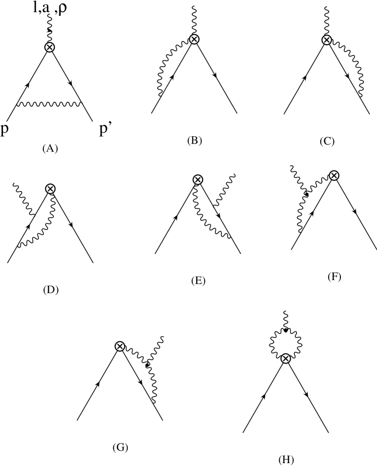
Figure 1: Feynman diagrams for $\Gamma_{R_{2}}^{\psi\overline{\psi}A}$

The Feynman diagrams contributing to these Green’s functions are in Fig.1. The one-loop radiative corrections lead to

$$(\Gamma_{R_{2}}^{\psi\overline{\psi}A})_{\mbox{1-loop}} = \left\{1+\frac{1}{\varepsilon}\frac{g_{B}^{2}}{16\pi^{2}}[-\frac{3}{4}C_{2}(G)]\right\}ig_{B}\varepsilon_{\sigma\rho\alpha\beta}l^{\alpha}\gamma^{\beta}T^{a}$$

$$+ \frac{1}{\varepsilon}\frac{g_{B}^{2}}{16\pi^{2}}[-\frac{3}{5}C_{2}(R)+\frac{1}{4}C_{2}(G)]g_{B}\gamma_{5}\gamma_{\sigma}(p+p^{\prime})_{\rho}T^{a}$$

$$+ \frac{1}{\varepsilon}\frac{g_{B}^{2}}{16\pi^{2}}[\frac{1}{3}C_{2}(R)-\frac{1}{4}C_{2}(G)]g_{B}\gamma_{5}\gamma_{\rho}(p+p^{\prime})_{\sigma}T^{a}$$

$$+ \frac{1}{\varepsilon}\frac{g_{B}^{2}}{16\pi^{2}}\frac{1}{3}C_{2}(R)g_{B}\gamma_{5}g_{\sigma\rho}(\not{\!p}+\not{\!p^{\prime}})T^{a}.$$

It should be noted that the tensor structure $ig_{B}\varepsilon_{\sigma\rho\alpha\beta}l^{\alpha}\gamma^{\beta}T^{a}$ is also included in $\left(\Gamma_{E_{1}^{\sigma}}^{\psi\overline{\psi}A}\right)_{\rm tree}$ and $\left(\Gamma_{E_{3}^{\sigma}}^{\psi\overline{\psi}A}\right)_{\rm tree}$. So we can not connect directly the coefficient of the first line of (3) with the renormalization constant of $R_{2}$. We need to separate this coefficient into the $R_{2}$-part and the EOM-parts. In this sense EOM operators also contribute to the physical quantity $\gamma_{NS}$. Rearranging the results of (3) properly, we obtain;

$$(\Gamma_{R_{2}}^{\psi\overline{\psi}A})_{\mbox{1-loop}} = \left\{1+\frac{1}{\varepsilon}\frac{g_{B}^{2}}{16\pi^{2}}[-\frac{5}{3}C_{2}(R)+C_{2}(G)]\right\}(\Gamma_{R_{2}}^{\psi\overline{\psi}A})_{\mbox{tree}}$$

$$+ \frac{1}{\varepsilon}\frac{g_{B}^{2}}{16\pi^{2}}[-\frac{4}{3}C_{2}(R)+\frac{1}{4}C_{2}(G)](\Gamma_{E_{1}}^{\psi\overline{\psi}A})_{\mbox{tree}}$$

$$+ \frac{1}{\varepsilon}\frac{g_{B}^{2}}{16\pi^{2}}[-\frac{2}{3}C_{2}(R)+\frac{1}{4}C_{2}(G)](\Gamma_{E_{2}}^{\psi\overline{\psi}A})_{\mbox{tree}}$$

$$+ \frac{1}{\varepsilon}\frac{g_{B}^{2}}{16\pi^{2}}\frac{1}{3}C_{2}(R)(\Gamma_{E_{3}}^{\psi\overline{\psi}A})_{\mbox{tree}}.$$

Now we introduce renormalization constants as follows:

$$A_{B}^{\mu}=Z_{3}^{1/2}A_{R}^{\mu},\hskip 28.45274pt\psi_{B}=Z_{2}^{1/2}\psi_{R},\hskip 28.45274ptg_{B}=Z_{g}g_{R}=Z_{1}Z_{3}^{-3/2}g_{R}.$$ (19)

The composite operators are renormalized as

$$(O_{i})_{R}=\sum_{j}Z_{ij}(O_{j})_{B},$$ (20)

and the Green’s functions of the composite operators with $\psi$, $\overline{\psi}$ and $A$ as the external lines are renormalized as follows:

$${\left(\Gamma_{O_{i}}\right)}_{R}=\sum_{j}Z_{2}\sqrt{Z_{3}}Z_{ij}\left(\Gamma_{O_{j}}\right)_{B}.$$ (21)

For example, $\left(\Gamma_{R_{2}}\right)_{R}$ reads

$$\left(\Gamma_{R_{2}}\right)_{R} = Z_{2}Z_{3}^{1/2}\left[Z_{11}\left\{\left(1+\frac{\widehat{\alpha}}{\varepsilon}(-\frac{5}{3}C_{2}(R)+C_{2}(G))\right)\left(\Gamma_{R_{2}}\right)_{\mbox{tree}}\right.\right.$$ (22)

$$+ \frac{\widehat{\alpha}}{\varepsilon}(-\frac{4}{3}C_{2}(R)+\frac{1}{4}C_{2}(G))\left(\Gamma_{E_{1}}\right)_{\mbox{tree}}$$

$$+ \frac{\widehat{\alpha}}{\varepsilon}(-\frac{2}{3}C_{2}(R)+\frac{1}{4}C_{2}(G))\left(\Gamma_{E_{2}}\right)_{\mbox{tree}}$$

$$+ \left.\frac{\widehat{\alpha}}{\varepsilon}\frac{1}{3}C_{2}(R)\left(\Gamma_{E_{3}}\right)_{\mbox{tree}}\right\}$$

$$+ \frac{\widehat{\alpha}}{\varepsilon}z_{12}\left(\Gamma_{E_{1}}\right)_{\mbox{tree}}+\frac{\widehat{\alpha}}{\varepsilon}z_{13}\left(\Gamma_{E_{2}}\right)_{\mbox{tree}}+\left.\frac{\widehat{\alpha}}{\varepsilon}z_{14}\left(\Gamma_{E_{3}}\right)_{\mbox{tree}}\right],$$

where $\widehat{\alpha}\equiv\displaystyle{\frac{g_{R}^{2}}{16\pi^{2}}}$. Since we have in the Feynman gauge

$$Z_{2}Z_{3}^{1/2}=\left\{1-\frac{\widehat{\alpha}}{\varepsilon}[C_{2}(R)+C_{2}(G)]\right\}g_{R}g_{B}^{-1},$$ (23)

the above equation (22) becomes

$$\left(\Gamma_{R_{2}}\right)_{R} = 1+\frac{\widehat{\alpha}}{\varepsilon}[z_{11}-\frac{8}{3}C_{2}(R)]\left(\Gamma_{R_{2}}^{g_{R}}\right)_{\mbox{tree}}$$ (24)

$$+ \frac{\widehat{\alpha}}{\varepsilon}(z_{12}-\frac{4}{3}C_{2}(R)+\frac{1}{4}C_{2}(G))\left(\Gamma_{E_{1}}^{g_{R}}\right)_{\mbox{tree}}$$

$$+ \frac{\widehat{\alpha}}{\varepsilon}(z_{13}-\frac{2}{3}C_{2}(R)+\frac{1}{4}C_{2}(G))\left(\Gamma_{E_{2}}^{g_{R}}\right)_{\mbox{tree}}$$

$$+ \frac{\widehat{\alpha}}{\varepsilon}(z_{14}+\frac{1}{3}C_{2}(R))\left(\Gamma_{E_{3}}^{g_{R}}\right)_{\mbox{tree}},$$

which should be finite. $z_{ij}$ is defined as,

$$Z_{ij}\equiv\delta_{ij}+\frac{\widehat{\alpha}}{\varepsilon}z_{ij},$$ (25)

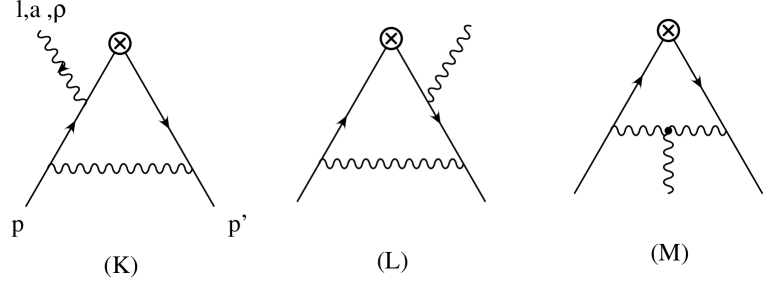
Figure 2: Additional diagrams for $\Gamma_{E_{i}}^{\psi\overline{\psi}A}$

and $(\Gamma^{g_{R}}_{R_{2}})_{\rm tree}$ denotes $(\Gamma_{R_{2}})_{\rm tree}$ with $g_{B}$ replaced by $g_{R}$. For $\Gamma_{E_{i}}^{\psi\overline{\psi}A}$, there are additional diagrams due to tree quark-antiquark vertices (Fig.2).

$$\left(\Gamma_{E_{1}}\right)_{R} = Z_{2}Z_{3}^{1/2}\left[Z_{22}\left(\Gamma_{E_{1}}\right)_{B}+Z_{23}\left(\Gamma_{E_{2}}\right)_{B}+Z_{24}\left(\Gamma_{E_{3}}\right)_{B}\right]$$ (26)

$$= 1+\frac{\widehat{\alpha}}{\varepsilon}[z_{22}-C_{2}(R)-\frac{1}{2}C_{2}(G)]\left(\Gamma_{E_{1}}^{g_{R}}\right)_{\mbox{tree}}$$

$$+ \frac{\widehat{\alpha}}{\varepsilon}[z_{23}+2C_{2}(R)+\frac{1}{4}C_{2}(G)]\left(\Gamma_{E_{2}}^{g_{R}}\right)_{\mbox{tree}}$$

$$+ \frac{\widehat{\alpha}}{\varepsilon}[z_{24}-C_{2}(R)-\frac{3}{8}C_{2}(G)]\left(\Gamma_{E_{3}}^{g_{R}}\right)_{\mbox{tree}}.$$

Further, the EOM operators like $E_{2}$ and $E_{3}$ which are of the form $E=\overline{\psi}B\displaystyle{\frac{\delta S}{\delta\overline{\psi}}}$, where $B$ is independent of fields, do not get renormalized [9]. This can be seen as follows.

$$Z_{2}Z_{3}^{-1/2}\langle 0|T\left(\psi(x_{1})A_{\rho}^{a}(x_{2})\overline{\psi}(x_{3})\overline{\psi}B\displaystyle{\frac{\delta S}{\delta\overline{\psi}}}(y)\right)|0\rangle$$

$$\hskip 36.98866pt=-iZ_{2}Z_{3}^{-1/2}\int{\cal{D}}\psi{\cal{D}}\overline{\psi}{\cal{D}}A\psi(x_{1})A_{\rho}^{a}(x_{2})\overline{\psi}(x_{3})\overline{\psi}B\displaystyle{\frac{\delta e^{iS}}{\delta\overline{\psi}}}(y)$$

$$\hskip 36.98866pt=-iZ_{2}Z_{3}^{-1/2}\int{\cal{D}}\psi{\cal{D}}\overline{\psi}{\cal{D}}A\left\{\psi(x_{1})A_{\rho}^{a}(x_{2})\overline{\psi}(x_{3})Be^{iS}\delta^{4}(0)\right.$$ (27)

$$\hskip 170.71652pt\left.+\psi(x_{1})A_{\rho}^{a}(x_{2})\overline{\psi}(y)e^{iS}\delta^{4}(y-x_{3})\right\}$$

$$\hskip 36.98866pt=-iZ_{2}Z_{3}^{-1/2}\langle 0|T\left(\psi(x_{1})A_{\rho}^{a}(x_{2})\overline{\psi}B(y)\right)|0\rangle\delta^{4}(y-x_{3}),$$

where the last equality holds as $\delta^{4}(0)$ vanishes in the sense of dimensional regularization. If $B$ does not contain any field, the RHS of (3) becomes finite by the wave functional renormalization for $\psi,\overline{\psi},A$. Therefore $E=\overline{\psi}B\displaystyle{\frac{\delta S}{\delta\overline{\psi}}}$ is a finite operator. Explicit calculations also indicate

$$\left(\Gamma_{E_{2}}\right)_{R}=Z_{2}Z_{3}^{1/2}Z_{33}\left(\Gamma_{E_{2}}\right)_{B}=\left(1+\frac{\widehat{\alpha}}{\varepsilon}z_{33}\right)\left(\Gamma_{E_{2}}^{g_{R}}\right)_{\mbox{tree}},$$ (28)

and

$$\left(\Gamma_{E_{3}}\right)_{R}=Z_{2}Z_{3}^{1/2}Z_{44}\left(\Gamma_{E_{3}}\right)_{B}=\left(1+\frac{\widehat{\alpha}}{\varepsilon}z_{44}\right)\left(\Gamma_{E_{3}}^{g_{R}}\right)_{\mbox{tree}}.$$ (29)

From the finiteness of (22), (26), (28), (29), we get the following results for the renormalization constants:

$$\begin{array}[]{ll}z_{11}={8\over 3}C_{2}(R),&z_{12}={4\over 3}C_{2}(R)-{1\over 4}C_{2}(G),\\ z_{13}={2\over 3}C_{2}(R)-{1\over 4}C_{2}(G),&z_{14}=-{1\over 3}C_{2}(R),\\ z_{22}=C_{2}(R)+{1\over 2}C_{2}(G),&z_{23}=-2C_{2}(R)-{1\over 4}C_{2}(G),\\ z_{24}=C_{2}(R)+{3\over 8}C_{2}(G),&z_{33}=z_{44}=0.\end{array}$$ (34)

This result is in agreement with the general theorem on the renormalization mixing matrix [8, 9, 15]. We should note that gauge variant EOM operator is also necessary to renormalize the physical operator.

We now determine the anomalous dimension of $R_{2}^{\sigma}$ operator. In physical matrix elements, the EOM operators do not contribute and we have

$$\langle\mbox{phys}|(R_{2}^{\sigma})_{B}|\mbox{phys}\rangle = Z_{11}^{-1}\langle\mbox{phys}|(R_{2}^{\sigma})_{R}|\mbox{phys}\rangle$$ (35)

$$= \left[1-\frac{g^{2}}{16\pi^{2}}\frac{1}{\epsilon}\frac{8}{3}C_{2}(R)\right]\langle\mbox{phys}|(R_{2}^{\sigma})_{R}|\mbox{phys}\rangle.$$

Therefore the anomalous dimension $\gamma_{NS}$ turns out to be

$$\gamma_{NS}(g) \equiv Z_{11}\mu\frac{d}{d\mu}(Z_{11}^{-1})$$ (36)

$$= \frac{g^{2}}{16\pi^{2}}\cdot 2z_{11}+O(g^{4})$$

$$= \frac{g^{2}}{16\pi^{2}}\gamma_{NS}^{0}+O(g^{4}),$$

and

$$\gamma_{NS}^{0}=2z_{11}=\frac{16}{3}C_{2}(R),$$ (37)

which coincides with the result obtained by Shuryak and Veinshtein [10] using the background field method.

Including the twist-4 effect the Bjorken sum rule becomes

$$\int_{0}^{1}dx\left[g_{1}^{p}(x,Q^{2})-g_{1}^{n}(x,Q^{2})\right]$$ (38)

$$= \frac{1}{6}\left\{g_{A}\left(1-\frac{\alpha_{s}(Q^{2})}{\pi}+{\cal O}(\alpha_{s}^{2})\right)-\frac{8}{9Q^{2}}f_{3}\left(\frac{\log{Q^{2}}/\log{\Lambda^{2}}}{\log{Q^{2}_{0}}/\log{\Lambda^{2}}}\right)^{\displaystyle{-32/9\beta_{0}}}\right\},$$

in the case of QCD.

4 Flavor singlet part

So far we have considered the flavor non-singlet part. Now we turn to the flavor singlet component. We should generally take account of gluon operators and BRS-exact operators as well in this case.
At first we see whether there exists other physical operators in addition to $R_{2}$. The possible twist-4 and spin-1 operators are the following:

$$\widetilde{G}^{\alpha}_{\mu}\hat{D}^{\sigma}G^{\mu}_{\alpha}=\widetilde{G}^{\alpha}_{\mu}\hat{D}^{[\sigma}G^{\mu]}_{\alpha}+\widetilde{G}^{\alpha}_{\mu}\hat{D}^{\mu}G^{\sigma}_{\alpha}=0,$$

$$\widetilde{G}^{\alpha}_{\mu}\hat{D}^{\mu}G^{\sigma}_{\alpha}=0\quad\mbox{(from Bianchi identity)},$$

$$\widetilde{G}^{\alpha\sigma}\hat{D}^{\mu}G_{\mu\alpha}\equiv R_{3},$$ (39)

where $\hat{D}_{\mu}^{ab}\equiv\partial_{\mu}\delta^{ab}+f^{abc}T^{c}$. Further, $R_{3}$, a gluon EOM operator and a BRS-exact operator may enter into the mixing.

$$E_{4} \equiv \widetilde{G}^{\alpha\sigma}\hat{D}^{\mu}G_{\mu\alpha}+\frac{1}{\alpha}\widetilde{G}^{\alpha\sigma}\partial_{\alpha}(\partial A)-gf^{abc}\widetilde{G}^{\alpha\sigma}_{a}(\partial_{\alpha}\xi_{b}\omega_{c})-g\overline{\psi}\widetilde{G}^{\alpha\sigma}\gamma_{\alpha}\psi,$$

$$A \equiv \frac{1}{\alpha}\widetilde{G}^{\alpha\sigma}\partial_{\alpha}(\partial A)-gf^{abc}\widetilde{G}^{\alpha\sigma}_{a}(\partial_{\alpha}\xi_{b}\omega_{c}).$$ (40)

Then we have a trivial relation among them,

$$R_{3}=E_{4}+R_{2}-A.$$ (41)

Therefore it happens that the physical operator is still only $R_{2}$ even in the flavor singlet case. This is characteristic to the lowest-spin case of higher-twist, in which only a few tensor structures are possible.

It should be noted that we have only to consider the mixing between $R_{2}^{\sigma}$ and

$$E_{G}^{\sigma}=\widetilde{G}^{\alpha\sigma}\hat{D}^{\mu}G_{\mu\alpha}-g\overline{\psi}\gamma_{\alpha}\widetilde{G}^{\alpha\sigma}\psi,$$ (42)

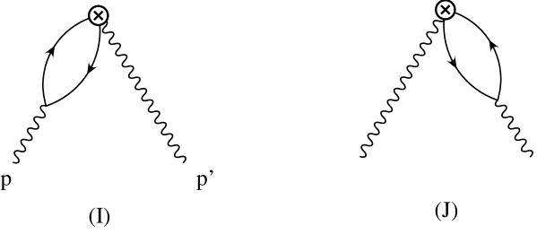
Figure 3: Feynman diagrams for $\Gamma_{R_{2}}^{AA}$

as long as we want to obtain the physical matrix element $Z_{11}^{S}$ where we do not have to consider Green’s functions with ghost operators in their external legs [18].
The mixing between $R_{2}$ and $E_{G}$ can be studied by computing the Green’s functions with two-gluon external lines shown in Fig.3. Then we have

$$\Gamma_{R_{2}}^{AA}(q)=\frac{1}{\varepsilon}\frac{g_{B}^{2}}{16\pi^{2}}(-\frac{2}{3}N_{f})\times\left(\Gamma_{E_{G}}^{AA}\right)_{\mbox{tree}},$$ (43)

where $N_{f}$ denotes the number of fermions. $\left(\Gamma_{E_{G}}^{AA}\right)_{\mbox{tree}}$ is given by

$$\left(\Gamma_{E_{G}}^{AA}\right)_{\mbox{tree}}=i\varepsilon^{\sigma\rho\alpha\beta}q_{\alpha}(q^{2}g_{\beta\lambda}-q_{\beta}q_{\lambda})-i\varepsilon^{\sigma\lambda\alpha\beta}q_{\alpha}(q^{2}g_{\beta\rho}-q_{\beta}q_{\rho}).$$ (44)

Now we introduce the renormalization constant $Z_{15}$ as

$$\left(R_{2}\right)_{R}=Z_{11}\left(R_{2}\right)_{B}+Z_{12}\left(E_{1}\right)_{B}+Z_{13}\left(E_{2}\right)_{B}+Z_{14}\left(E_{3}\right)_{B}+Z_{15}\left(E_{G}\right)_{B}.$$ (45)

So we get

$$\left(\Gamma_{R_{2}}^{AA}\right)_{R} = Z_{3}\left[Z_{11}\left(\Gamma_{R_{2}}^{AA}\right)_{B}+\sum_{i=1}^{3}Z_{1i}\left(\Gamma_{E_{i}}^{AA}\right)_{B}+Z_{15}\left(\Gamma_{E_{G}}^{AA}\right)_{B}\right]$$ (46)

$$\sim \frac{\widehat{\alpha}}{\varepsilon}(-\frac{2}{3}N_{f})\left(\Gamma_{E_{G}}^{AA}\right)_{\mbox{tree}}+Z_{15}\left(\Gamma_{E_{G}}^{AA}\right)_{\mbox{tree}}.$$

From the finiteness of the above expression, we have

$$Z_{15}=\frac{\widehat{\alpha}}{\varepsilon}\times\frac{2}{3}N_{f}.$$ (47)

On the other hand, the relation (21) becomes

$$\left(R_{2}^{\psi\overline{\psi}A}\right)_{R}=Z_{2}Z_{3}^{1/2}\left[Z_{11}\left(\Gamma_{R_{2}}^{\psi\overline{\psi}A}\right)_{B}+\sum_{i=1}^{3}Z_{1i}\left(\Gamma_{E_{i}}^{\psi\overline{\psi}A}\right)_{B}+Z_{15}\left(\Gamma_{E_{G}}^{\psi\overline{\psi}A}\right)_{B}\right],$$ (48)

in this case. Since $(\Gamma^{\psi\overline{\psi}A}_{R_{2}})_{B}$ is just the same as the flavor non-singlet case, we can easily extract $Z_{11}^{S}$ from the result of $Z_{11}^{NS}$.

$$Z_{11}^{S}=Z_{11}^{NS}+\frac{2}{3}N_{f},$$ (49)

namely,

$$\gamma_{S}^{0}=\gamma_{NS}^{0}+\frac{4}{3}N_{f},$$ (50)

hence we obtain the exponent for the singlet part

$$-\frac{\gamma_{S}^{0}}{2\beta_{0}}=-\frac{\gamma_{NS}^{0}}{2\beta_{0}}-\frac{2}{3}\frac{N_{f}}{\beta_{0}}=-\frac{1}{\beta_{0}}\left(\frac{32}{9}+\frac{2}{3}N_{f}\right).$$ (51)

Again we reproduce the result of [10]. Substituting these results into (5), we get

$$\delta\Gamma_{\rm tw-4}^{\rm singlet}=\frac{C^{\rm twist-4}}{Q^{2}}\left(\frac{\log{Q^{2}}/\log{\Lambda^{2}}}{\log{Q_{0}^{2}}/\log{\Lambda^{2}}}\right)^{-(32/9\beta_{0}+2N_{f}/3)},$$ (52)

where $C^{\rm twist-4}$ denotes the coefficients including the reduced matrix elements, $f_{i}$.

5 Concluding remarks

In this paper, we have investigated the renormalization of the twist-4 operators relevant for the Bjorken and Ellis-Jaffe sum rules. We obtained the anomalous dimensions by considering off-shell Green’s functions in which the role of EOM operators was important. We have also seen that the renormalization matrix satisfies the general theorems for the renormalization of composite operators in the gauge theory. Since there appears only one physical operator, our case seems to be the simplest example which contains non-trivial structures.

Phenomenologically whether the twist-4 effects has significant contributions depends on the value of their reduced matrix elements. Estimations of their values were given by various methods. For example, from the QCD sum rules [19], $\delta\Gamma_{1}^{p-n}$ amounts to about 4% of $\Gamma_{1}^{p-n}$, and the chiral-bag model [20] predicts similar value, but some other estimations predict twice or much larger values [21]. Furthermore the reduced matrix elements of twist-4 operators are considered to be related to the renormalon ambiguity of the coefficient functions of the leading twist parts [22]. So we can not give any definite predictions about the reduced matrix elements until some consistent treatments are developed for these problems. On the other hand, the anomalous dimensions of twist-4 operators are free from the renormalon ambiguity and have definite values.

The numerical values of the exponents of log-terms in $\delta\Gamma_{1}^{p,n}$ are so small that the $\log{Q^{2}}$ scalings are quite hard to observe in experiments. Since the anomalous dimensions are considered to become large as the spin of the operators increases, the scaling of the twist-4 terms are probably easier to measure in some higher moments . However to obtain the anomalous dimensions in spin-n case by our method is not so easy because many gauge variant EOM operators may enter into the operator mixing. In the twist-4 case, it is hard to simplify these structures by the method used in the twist-3 case [23, 24] in which many tree amplitude of different EOM operators are projected out to a single one by a null vector $\Omega_{\rho}$. Since the twist-4 operators have a pair of Lorentz indices contracted, there still remain so many independent tree amplitudes after the contraction by $\Omega_{\rho}$ and this complicates the situation. So we need some further developments in the techniques to disentangle the mixing problem.

We are very grateful to J.Kodaira, T.Uematsu and Y.Yasui for valuable discussions. Thanks are also due to T.Uematsu for careful reading of the manuscript.