NLO predictions for the growth of $F_{2}$ at small $x$ and comparison with experimental data

C. LΓ³pez, F. Barreiro and F.J. YndurΓ‘in
Departamento de Fisica TeΓ³rica, C-XI
Universidad AutΓ³noma de Madrid, Madrid, Spain
Abstract

We present parametrizations for the proton structure function $F_{2}$ in the next to leading order in perturbative QCD. The calculations show that the dominant term to $F_{2}(x,Q^{2})$ should grow as $x^{-\lambda_{S}}$ for small $x$ values, with the exponent $\lambda_{S}$ being essentially independent of $Q^{2}$. Comparisons with the most recent H1 and ZEUS data confirm the value $\lambda_{S}\sim 0.35$ obtained previously from fits to low energy data.

1 Introduction

One of the most interesting results obtained at HERA so far, has to do with the dramatic increase of the proton structure function $F_{2}$ at low Bjorken $x$ values [1] and [2]. The precision of these measurements do allow the extraction of the gluon density in the proton down to $x\sim 10^{-3}$ [3] and [4].
Although the general framework to discuss deep inelastic scattering is established and well known since two decades, the interpretation of these data is subject to some controversy. Two lines of thought are generally followed to describe the data.

  • β€’

    On the one hand, there are those who advocate that this dramatic increase of the proton structure function can be obtained from singular [5, 6] (non-singular [7]) parton densities at moderate $Q^{2}_{0}\sim~{}4~{}GeV^{2}$ (resp. at very small $Q^{2}_{0}\sim~{}0.5~{}GeV^{2}$), which are then evolved using the well known DGLAP equations [8]. This procedure describes the experimental data very well at the cost of having approximately twenty parameters which enter into the parametrization of valence and sea quark, as well as gluon densities at an input $Q_{0}^{2}$ value, in addition to assumptions about their functional forms.

  • β€’

    On the other hand, there are those who argue that since at very low $x$ values, the boson gluon fusion mechanism is the dominant source of leading order (LO) corrections to the Born level cross sections and the kernel $P_{g}\rightarrow gg$ is singular, one expects that when including higher order QCD corrections, one would have to sum multigluon exchange ladders. Depending on the approximation used to perform this sum, one encounters deviations from the DGLAP linear evolution equations. In fact, the proponents of this approach claim that at fixed $Q^{2}$ the x-dependence is most generally given by the BFKL equations [9], which predict the parton densities to behave like $x^{-\omega}$ with

    $$\omega=\frac{12\log 2}{\pi}\alpha_{s}(Q^{2})\sim 0.5$$ (1)

    for $Q^{2}\sim 20~{}GeV^{2}$. However, theory does not tell us where in the $(Q^{2},x)$ plane the transition region lies beyond which the expansion in terms of $\log\frac{1}{x}$ is important. The BFKL evolution equations are not yet numerically implemented in the parametrizations discussed above.

We think that in order to clarify the issue one should try

  • β€’

    to search for specific fingerprints of the BKFL equations, as discussed by Mueller [10] and others [11]. In particular since the above prediction runs contrary to the trend observed in the data [12].

  • β€’

    to make detailed comparisons between analytic NLO QCD predictions and experimental data to see if one can isolate regions of phase space where discrepancies might appear. In this context, we would like to remind the reader that since the behaviour at small $x$ of the proton structure function is connected with the singularities of the operator product expansion matrix elements, one has two specific predictions, depending on whether these singularities lie to the left or to the right of those of the anomalous dimension matrix [12], such that either

    • –

      the proton structure function should grow faster than a log but slower than a power in $x$ [13], i.e.

      $$F_{2}(x,Q^{2})\simeq C_{0}\left[\frac{33-2n_{f}}{576\pi^{2}|\log x|\log[\alpha_{s}(Q_{0}^{2})/\alpha_{s}(Q^{2})]}\right]^{\frac{1}{4}}\exp\sqrt{\frac{144|\log x|}{(33-2n_{f})}\;\left[\log\frac{\alpha_{s}(Q_{0}^{2})}{\alpha_{s}(Q^{2})}\right]}$$ (2)

      leading to a double asymptotic behaviour as discussed by Ball and Forte [14]

    • –

      or else the proton structure function should behave as a power in $x$ i.e. $x^{-\lambda_{S}}$ with $\lambda_{S}$ a $Q^{2}$ $\it independent$ constant except for possible variations due to crossing flavour thresholds which could depend on $Q^{2}$ [15], [17] and [16]. This behaviour is the same as that calculated by Witten for $\gamma^{*}\gamma$ scattering [18].

    The purpose this paper is to test this second set of predictions, which date as far back as 1980 [19] and dwell upon the possibility that the cross sections for off-shell particles grow as a power of centre of mass energy [20], see also [26]. This is particularly interesting, since it has been shown that although the double asymptotic behaviour is a dominant feature of the data, there appear non-negligible scaling violation effects [22].

Our aim is twofold

  • *

    to present NLO parametrizations for $F_{2}$ and make extensive comparisons with the most recent data [22] and [23].

  • *

    to extract the gluon density in the HERA kinematic regime and to present predictions for $R(x,Q^{2})$ which will be measured soon at HERA.

2 LO and NLO predictions

Perturbative QCD provides evolution equations for the structure functions, in such a way that if we know them at a given $Q^{2}_{0}$, we can predict them at any other $Q^{2}$ value, assuming that both $Q^{2}_{0}$ and $Q^{2}$ lie in a range where perturbation theory applies.
The DGLAP equations represent one of the forms in which the evolution in $Q^{2}$ can be expressed, whereas the most direct result of the operator product expansion (OPE) approach is expressed in terms of moments of structure functions. Both approaches are equivalent.
Once we know the evolution equations, the goal will be to find the functional form $F(x,Q^{2})$ for the structure functions such that used at an input $Q^{2}_{0}$, the resulting β€˜evolved’ function would continue to be the same $F(x,Q^{2})$ simply calculated at the new $Q^{2}$ value. No such functional form has been found so far, thus any simple analytical form chosen as input is not invariant as a function of $Q^{2}$, in contradiction with the fact that any other value $Q^{2}_{1}$ could have been chosen as the starting point for the evolution.
However, one can find functional forms compatible with QCD in definite $x$ regions; so we can give simple functional forms compatible with the DGLAP evolution equations, in particular the behaviour at the end points $x=0,1$ and certain sum rules. As a result, we know exact solutions to the DGLAP evolution equations, albeit only locally and not for the whole $x$ range. These results were derived in [19] and [24] at the leading (LO) and next to leading (NLO) order.
Let us consider $F_{2}(x,Q^{2})$ for DIS $e-p$ scattering. It can be written as

$$F_{2}(x,Q^{2})=F_{S}(x,Q^{2})+F_{NS}(x,Q^{2})$$ (3)

where $F_{S}(x,Q^{2})$ ($F_{NS}(x,Q^{2})$) refer to the singlet (resp. non-singlet) pieces, whose evolution equations are different. Indeed the singlet part and the gluon momentum density $F_{G}(x,Q^{2})$ evolve together, whereas the non-singlet part is decoupled from gluons and evolves independently.

2.1 LO predictions

To LO, the evolution of the moments takes a very simple form

$$\mu_{NS}(n,Q^{2})=\left(\frac{\alpha_{s}(Q^{2}_{0})}{\alpha_{s}(Q^{2})}\right)^{\bf d(n)}\cdot\mu_{NS}(n,Q_{0}^{2})$$ (4)

for the non-singlet piece and, for the singlet,

$$\vec{\mu}(n,Q^{2})=\left(\frac{\alpha_{s}(Q^{2}_{0}}{\alpha_{s}(Q^{2}}\right)^{\bf D(n)}\cdot\vec{\mu}(n,Q_{0}^{2})$$ (5)

where $\vec{\mu}(n,Q^{2})$ is the two-component vector

$$\vec{\mu}(n,Q^{2})=\left(\begin{array}[]{cc}\mu_{S}(n,Q^{2})\\ &\\ \mu_{G}(n,Q^{2})\end{array}\right)$$ (6)

defined as usual

$$\mu(n,Q^{2})=\int_{0}^{1}dxx^{n-2}F(x,Q^{2})$$ (7)

and $\bf d(n)$ and $\bf D(n)$ are proportional to the anomalous and anomalous dimension matrix, whose exact expressions are

$${\bf d(n)}=\frac{16}{33-2n_{f}}\left(\frac{1}{2n(n+1)}+\frac{3}{4}-S_{1}(n)\right)$$ (8)

and

$${\bf D(n)}=\frac{16}{33-2n_{f}}\left(\begin{array}[]{cc}\frac{1}{2n(n+1)}+\frac{3}{4}-S_{1}(n)&\frac{3n_{f}}{8}\frac{n^{2}+n+2}{n(n+1)(n+2)}\\ \frac{n^{2}+n+2}{2n(n^{2}-1)}&\frac{9}{4n(n-1)}+\frac{9}{4(n+1)(n+2)}+\frac{33-2n_{f}}{16}-\frac{9S_{1}(n)}{4}\end{array}\right)$$ (9)

where

$$S_{1}(n)=n\sum_{k}\frac{1}{k(k+n)}$$ (10)

and $n_{f}$ is the number of flavours.
From the fact that $Q^{2}_{0}$ and $Q^{2}$ are arbitrary values in the range of applicability of perturbation theory, it follows that the moments must be of the form

$$\mu_{NS}(n,Q^{2})=\left[\alpha_{s}(Q^{2})\right]^{-\bf d(n)}\cdot b_{NS}(n)$$ (11)

and

$$\vec{\mu}(n,Q^{2})=\left[\alpha_{s}(Q^{2})\right]^{-\bf D(n)}\cdot\vec{b}(n)$$ (12)

with $b_{NS}(n)$ and $\vec{b}(n)$ being independent of the squared momentum transfer.
If we try a Regge inspired functional form

$$F_{NS}(x,Q^{2})\begin{array}[t]{c}=\\ \stackrel{{\scriptstyle x\rightarrow 0}}{{}}\end{array}B_{NS}(Q^{2})\cdot x^{\lambda_{NS}(Q^{2})}$$ (13)

and

$$F_{S}(x,Q^{2})\begin{array}[t]{c}=\\ \stackrel{{\scriptstyle x\rightarrow 0}}{{}}\end{array}B_{S}(Q^{2})\cdot x^{-\lambda_{S}(Q^{2})}$$ (14)

for the structure functions near the end point $x=0$, the dependence of $B(Q^{2})$, $\lambda(Q^{2})$ upon $Q^{2}$ is related to the moments in Eqs. 11 and 12 for the value of $n$ at which they diverge.
The results which can be found in [24] and [19] are such that $\lambda_{NS}$ and $\lambda$ should be $Q^{2}$ independent. Furthermore one must have $\lambda_{NS}<1$ and $\lambda_{S}>0$, and

$$B_{NS}(Q^{2})=B_{NS}\cdot\left[\alpha_{s}(Q^{2})\right]^{-d(1-\lambda_{NS})}$$ (15)

and

$$B_{S}(Q^{2})=B_{S}\cdot\left[\alpha_{s}(Q^{2})\right]^{-d_{+}(1+\lambda_{S})}$$ (16)

In addition, the gluon structure function ought to be proportional to the singlet piece of the structure function i.e.

$$F_{G}(x,Q^{2})=B_{G}(Q^{2})\cdot x^{-\lambda_{S}}$$ (17)

with

$$B_{G}(Q^{2})=\frac{d_{+}(1+\lambda_{S})-D_{11}(1+\lambda_{S})}{D_{12}(1+\lambda_{S})}\cdot B_{S}(Q^{2})=B_{GS}\cdot B_{S}(Q^{2})$$ (18)

where by $d_{+}(n)$ we denote the largest eigenvalue of the anomalous dimension matrix $\bf{D(n)}$.

Refer to caption

Figure 1: The dependence on $\lambda$ of $B_{GS},v_{G}$ and $v_{S}$

2.2 NLO predictions

The extension of these results to the NLO is tedious, the result being of the form

$$B_{NS}(Q^{2})=B_{NS}\cdot\left[\alpha_{s}(Q^{2})\right]^{-d(1-\lambda_{NS})}\cdot\{1+\frac{\alpha_{s}(Q^{2})}{4\pi}\cdot v_{NS}(1-\lambda_{NS})\}$$ (19)
$$B_{S}(Q^{2})=B_{S}\cdot\left[\alpha_{s}(Q^{2})\right]^{-d_{+}(1+\lambda_{S})}\cdot\{1+\frac{\alpha_{s}(Q^{2})}{4\pi}\cdot v_{S}(1+\lambda_{S})\}$$ (20)

and

$$B_{G}(Q^{2})=B_{S}\cdot\left[\alpha_{s}(Q^{2})\right]^{-d_{+}(1+\lambda_{S})}\cdot\{B_{GS}+\frac{\alpha_{s}(Q^{2})}{4\pi}\cdot v_{G}(1+\lambda_{S})\}$$ (21)

with $v_{NS}(1-\lambda_{NS})$, $v_{S}(1+\lambda_{S})$ and $v_{G}(1+\lambda_{S})$ being known functions of the exponents $\lambda_{NS}$ and $\lambda_{S}$ given in [24] 111Note that there are a few typographical errors in this reference, they will be corrected in a forthcoming publication by K. Adel and F.J. YndurΓ‘in.
The last two of these functions have been fitted to simple rational expressions and the results for $n_{f}=3,4$ are presented in Fig. 1 together with similar fits to $B_{GS}$ which is defined in Eq. 18 as the proportionality factor to LO between $B_{G}(Q^{2})$ and $B_{S}(Q^{2})$.
An important comment to make is that, NLO corrections to the singlet and gluon structure functions are large, in contrast to the situation for the non-singlet case. To be rigorous one would have to replace Eqs. 20 and 21 by the more precise exponential forms that follow from the evolution equation, and of which Eqs. 19-21 are an approximation.
Note that the gluon structure function, at the end point $x=0$, is completely determined by the quark singlet structure function which in turn is the dominant piece of $F_{2}(x,Q^{2})$. In fact,

$$F_{G}(x,Q^{2})\begin{array}[t]{c}=\\ \stackrel{{\scriptstyle x\rightarrow 0}}{{}}\end{array}\frac{B_{GS}+\frac{\alpha_{s}}{4\pi}\cdot v_{G}(1+\lambda_{S})}{1+\frac{\alpha_{s}}{4\pi}\cdot v_{S}(1+\lambda_{S})}\cdot F_{S}(x,Q^{2})$$ (22)

Since $F_{S}(x,Q^{2})$ is defined in terms of quark densities in the proton as

$$F_{S}(x,Q^{2})=<e_{i}^{2}>\sum_{i}x\cdot q_{i}(x,Q^{2})$$ (23)

where the sum runs over quark flavours with charge given by $e_{i}$. The gluon density is then given by

$$xG(x,Q^{2})=\frac{1}{<e_{i}^{2}>}\cdot F_{G}(x,Q^{2})$$ (24)

Let us now turn to a discussion of the limit $x\rightarrow 1$. We have considered the ansatz

$$F(x,Q^{2})\begin{array}[t]{c}=\\ \stackrel{{\scriptstyle x\rightarrow 1}}{{}}\end{array}A(Q^{2})\cdot(1-x)^{\nu(Q^{2})}$$ (25)

The dependence of the functions $A(Q^{2})$ and $\nu(Q^{2})$ is now related to the evolution of the moments in the limit $n\rightarrow\infty$. One finds

$$A_{NS}(Q^{2})=A_{NS}\cdot\left[\alpha_{s}(Q^{2})\right]^{-d_{0}}\cdot\frac{\Gamma(1+\nu_{0})}{\Gamma(1+\nu(Q^{2}))}$$ (26)
$$A_{S}(Q^{2})=A_{S}\cdot\left[\alpha_{s}(Q^{2})\right]^{-d_{0}}\cdot\frac{\Gamma(1+\nu_{0})}{\Gamma(1+\nu(Q^{2}))}$$ (27)

with

$$\nu(Q^{2})=\nu_{0}-\frac{16}{33-2n_{f}}\cdot log~{}\alpha_{s}(Q^{2})$$ (28)

and

$$d_{0}=\frac{16}{33-2n_{f}}\cdot\{\frac{3}{4}-\gamma_{E}\}$$ (29)

with $\gamma_{E}$ Euler’s constant.
The gluon momentum density is fully determined, also in this limit, by the singlet structure function:

$$F_{G}(x,Q^{2})=\frac{2}{5}A_{S}(Q^{2})\cdot\frac{(1-x)^{\nu(Q^{2})+1}}{(\nu(Q^{2})+1)\cdot log\frac{1}{1-x}}$$ (30)

Finally from the fact that $d(1)=0$ and $d_{+}(2)=0$, the following sum rules can be derived

$$\int_{0}^{1}x^{-1}\cdot F_{NS}(x,Q^{2})dx=\left(1-3<e_{i}^{2}>\right)\{1+\frac{k}{4\pi}\alpha_{s}(Q^{2})\}$$ (31)

with $k$ a known and very small constant [24] and

$$\int_{0}^{1}\{F_{S}(x,Q^{2})~{}+~{}F_{G}(x,Q^{2})\}dx=~{}<e_{i}^{2}>\cdot\{1-\frac{5}{9\pi}\alpha_{s}(Q^{2})\}$$ (32)

3 Parametrizations for the proton structure function

In this section, we give approximate parametrizations compatible with the exact conditions discussed above.

3.1 LO parametrizations

We consider the following ansatz for

$$F_{S}(x,Q^{2})=\{B_{S}(Q^{2})\cdot x^{-\lambda_{S}}~{}+~{}C_{S}(Q^{2})\}(1-x)^{\nu(Q^{2})}$$ (33)

where

$$B_{S}(Q^{2})=B_{S}\cdot\left[\alpha_{s}(Q^{2})\right]^{-d_{+}(1+\lambda_{S})}$$ (34)

and $\nu(Q^{2})$ given by Eq. 28.
The singlet part is the most important contribution at small $x$, so that the predicted behaviour near $x=0$ has to be implemented through the term $B_{S}(Q^{2})\cdot x^{-\lambda}$. Note from Eq. 33 that it is divergent when $x\rightarrow 0$ and that the coefficient $B_{S}(Q^{2})$ grows rapidly with $Q^{2}$, becoming asymptotically dominant. This part is responsible for the increase of the structure function at small $x$ as a function of $Q^{2}$ as observed experimentally.
On the other hand, in the limit $Q^{2}\rightarrow 0$ , $B_{S}(Q^{2})$ becomes negligible, in fact, it vanishes for $Q^{2}=0$. At small $Q^{2}$ we expect soft Pomeron-like contributions to remain. This term we parametrise phenomenologically with the help of the second piece in Eq. 33 proportional to $C_{S}(Q^{2})$, whose relative weight will decrease as a function of increasing $Q^{2}$ but remain important at low and intermediate $Q^{2}$ values.
We would like to remark that the dependence of both functions $B_{S}(Q^{2})$ and $C_{S}(Q^{2})$ can be determined by implementing the limits at $x=0,1$. Thus,

$$C_{S}(Q^{2})=~{}-B_{S}\cdot\left[\alpha_{s}(Q^{2})\right]^{-d_{+}(1+\lambda_{S})}~{}+~{}A_{S}\cdot\left[\alpha_{s}(Q^{2})\right]^{-d_{0}}\cdot\frac{\Gamma(1+\nu_{0})}{\Gamma(1+\nu(Q^{2}))}$$ (35)

For the non-singlet part we could try a parametrization of the form

$$F_{NS}(x,Q^{2})=\{B_{NS}(Q^{2})\cdot x^{-\lambda_{NS}}~{}+~{}C_{NS}(Q^{2})\cdot x\}\cdot(1-x)^{\nu(Q^{2})}$$ (36)

but since its contributions turns out to be small, we will use simply

$$F_{NS}(x,Q^{2})=~{}B_{NS}(Q^{2})\cdot x^{-\lambda_{NS}}\cdot(1-x)^{\nu(Q^{2})}$$ (37)

with

$$B_{NS}(Q^{2})=B_{NS}\left[\alpha_{s}(Q^{2})\right]^{-d_{0}}\frac{\Gamma(1+\nu_{0})}{\Gamma(1+\nu(Q^{2}))}$$ (38)

In Eq. 36, $\lambda_{NS}$ is related to the intercept of the leading Regge trajectory ($\rho$) contribution to this piece, $\lambda_{NS}=0.45$. In one wishes to restrict the number of free parameters, one can use Eq. 31 to obtain

$$B_{NS}(Q^{2})=\left(1-3\cdot<e_{i}^{2}>\right)\cdot\frac{\Gamma(1+\lambda_{NS}+\nu(Q^{2}))}{\Gamma(\lambda_{NS})\Gamma(1+\nu(Q^{2}))}$$ (39)

For the gluon momentum density, the prediction following from our analysis will be

$$F_{G}(x,Q^{2})=~{}\{B_{G}(Q^{2})\cdot x^{-\lambda_{S}}~{}+~{}C_{G}(Q^{2})\}\cdot(1-x)^{1+\nu(Q^{2})}$$ (40)

3.2 Parametrizations at the NLO

At the next to leading order, the only significant modification to the expressions given above refer to an extra term of the form $1+\frac{2\alpha_{s}}{3\pi}log^{2}(1-x)$ which will be significant only at large $x$. Therefore we have for the dominant singlet part

$$F_{S}(x,Q^{2})=\{B_{S}(Q^{2})\cdot x^{-\lambda_{S}}~{}+~{}C_{S}(Q^{2})\}(1-x)^{\nu_{1}(Q^{2})}\cdot\{1+\frac{2\alpha_{s}}{3\pi}log^{2}(1-x)\}$$ (41)

with $\nu_{1}(Q^{2})$ being given by the following expression

$$\nu_{1}(Q^{2})=\nu(Q^{2})-\alpha_{s}\{\frac{4}{3\pi}\psi(\nu(Q^{2})+1)+a_{1}\}$$ (42)

The coefficient $B_{S}(Q^{2})$ is given by Eq. 19, and $C_{S}(Q^{2})$ is such that Eq. 35 is satisfied i.e. including NLO terms

$$C_{S}(Q^{2})=~{}-B_{S}\cdot\left[\alpha_{s}(Q^{2})\right]^{-d_{+}(1+\lambda_{S})}~{}+~{}A_{S}\cdot\left[\alpha_{s}(Q^{2})\right]^{-d_{0}}\cdot\frac{e^{g(\alpha_{s})\alpha_{s}}\cdot\Gamma(1+\nu_{0})}{\Gamma(1+\nu(Q^{2}))}$$ (43)

with

$$g(\alpha_{s})=a_{0}+a_{1}\cdot\psi(1+\nu(Q^{2}))+\frac{2}{3\pi}\{\psi^{2}(1+\nu(Q^{2})-\psi^{\prime}(1+\nu(Q^{2}))\}$$ (44)

Here $\psi$ denotes the logarithmic derivative of the $\Gamma$ function, $a_{0}$ and $a_{1}$ are constants essentially independent of the number of flavours. Numerically $a_{0}=-1.18$ and $a_{1}=0.66$. For the non-singlet part we take

$$F_{NS}(x,Q^{2})=~{}B_{NS}(Q^{2})\cdot x^{-\lambda_{NS}}\cdot(1-x)^{\nu(Q^{2})}\cdot\{1+\frac{2\alpha_{s}}{3\pi}log^{2}(1-x)\}$$ (45)

with $B_{NS}(Q^{2})$ fixed in such a way so as to satisfy the sum rule given in Eq. 31, whose NLO corrections are negligible. These parametrizations are similar to those used by the authors of [25] to fit fixed targed lepton nucleon scattering data. At this point we would like to remark that these predictions are valid for a range in $Q^{2}$ where the number of flavours is fixed.

4 Comparison with experimental data

We can think of two possibilities to compare experimental data to theoretical predictions. The simplest is illustrated in our fits of the ’94 ZEUS shifted vertex data [21] to the expression given by Eqs. 14 and 20 in NLO. This has also been tried in [12]. In order to be in the kinematical region where this term dominates the singlet structure function, we restricted ourselves to Q2superscript𝑄2Q^{2} values above 3​G​e​V23𝐺𝑒superscript𝑉23~{}GeV^{2} and Bjorken xπ‘₯x below 0.010.010.01. The QCD scale parameter Ξ›M​SΒ―subscriptΛ¯𝑀𝑆\Lambda_{\bar{MS}} was fixed in a way be discussed below. The reason for this has to do with the fact that the normalization factor BSsubscript𝐡𝑆B_{S} and the strong coupling constant are tightly correlated. Therefore we prefer to fix the coupling constant to values measured elsewhere. The number of excited flavours was assumed to be constant and the quality of the fits are similar irrespective of whether we take nf=3subscript𝑛𝑓3n_{f}=3 or nf=4subscript𝑛𝑓4n_{f}=4. Disregarding the overall normalization factor, BSsubscript𝐡𝑆B_{S}, the relevant fitted parameter Ξ»Ssubscriptπœ†π‘†\lambda_{S} turns out to be 0.32Β±0.01plus-or-minus0.320.010.32\pm 0.01 for four excited flavours. The Ο‡2superscriptπœ’2\chi^{2} is 25 for 33 experimental points. The agreement between data 
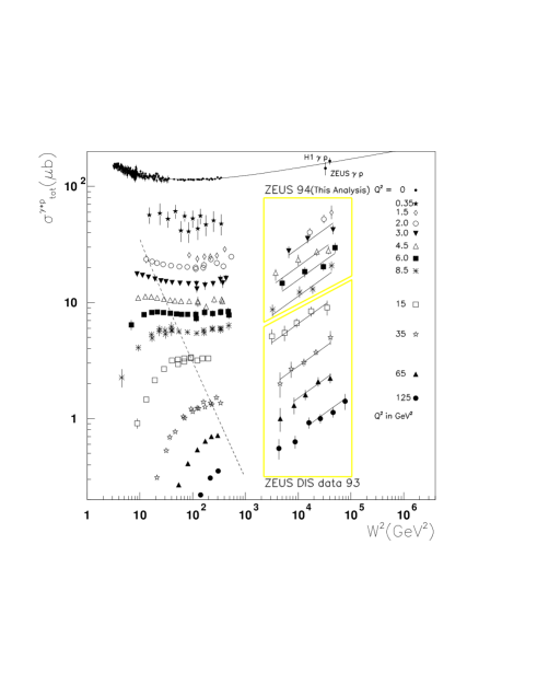
and NLO QCD predictions is quite good as illustrated in Fig. 2, even down to small Q2superscript𝑄2Q^{2} values where the applicability of perturbation theory could be questioned. The solid lines in Fig. 2 represent the results of the fits.

Refer to caption

Figure 2: The $\gamma^{*}-p$ cross-sections as a function of $W$

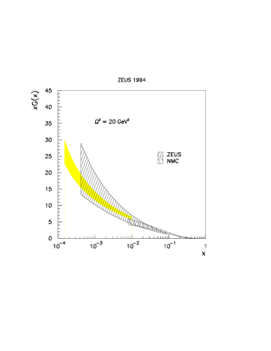
The gluon density extracted from these fits also agrees well with that obtained by ZEUS using the Ellis-Kunszt-Levin method [27], which relates the gluon density to the logarithmic derivative of the proton structure function, following a numerical approximation originally derived by [28]. Our results are shown in Fig. 3. Our smaller error band has to do with the fact that the gluon density determination within our formalism, is subject essentially only to the statistical errors of the proton structure function itself.
The criticism to the procedure developed so far is clear from Fig. 2. A fast rise of the cross section for virtual $\gamma$-p scattering is observed at large $W^{2}$ values, but this rise is sitting on top of a non-negligible plateau which moreover exhibits clear leading twist behaviour. Questions like, what is the dependence of $\lambda_{S}$ upon variations in the limits used to define the kinematical region over which the fits are done, or whether one should subtract from the low $x$ region a contribution smoothly coming from the large $x$ (i.e. small $W^{2}$) domain, have to be answered in a quantitative way.
In order to do this, we consider a different approach in which we have performed fits to the data in the whole $(x,Q^{2})$ region covered by the experiments. We would like to recall that four parameters are involved in our fits, if we consider a region in $Q^{2}$ with a fixed number of flavours, namely a coefficient $B_{S}$ to give the normalization of the singlet piece to $F_{2}$, a coefficient $A_{S}$ which serves to define the subleading contribution to the singlet piece, $\lambda_{S}$ which defines the growth rate for small $x$ and $\nu_{0}$ which fixes the behaviour of the structure function at large $x$ values. The strong coupling constant is fixed through $\Lambda_{\bar{MS}}=263~{}MeV$ for four flavours as given in [29]. The dependence of the QCD scale parameter on the number of flavours is taken as in [30]. Although reasonable fits can be obtained with $n_{f}=4$ independent of $Q^{2}$, we find that the quality of the fits improve by considering $n_{f}=3$ below $Q^{2}=10~{}GeV^{2}$, $n_{f}=4$ for $Q^{2}$ between $10~{}GeV^{2}$ and $100~{}GeV^{2}$ and $n_{f}=5$ above. In principle, $\lambda_{S}$ could be different for different number of excited quark flavours. Therefore, we have tried two sets of fits, one with $\lambda_{S}$ fixed for different quark flavours and a second one allowing different $\lambda_{S}$ values as a function of $n_{f}$. The second set of fits yield considerably improved $\chi^{2}$ values, and these are shown in the figures.

Refer to caption

Figure 3: The gluon density determined from shifted vertex ZEUS data, dotted band, compared with previous determinations.

We are aware that this is an approximation: for instance in the model of GRS the charm quark contribution rises smoothly with increasing $Q^{2}$. Once $F_{2}^{charm}$ is measured, this could be subtracted from the experimental $F_{2}$ values and we could keep $n_{f}$ fixed to $n_{f}=3$ in the complete $Q^{2}$ range. The effect of the bottom quark excitation, due to its smaller charge, is smaller. These are the main sources of uncertainty in our determination of the gluon density and of $R(x,Q^{2})$ which we cannot take into account in a model independent way right now.
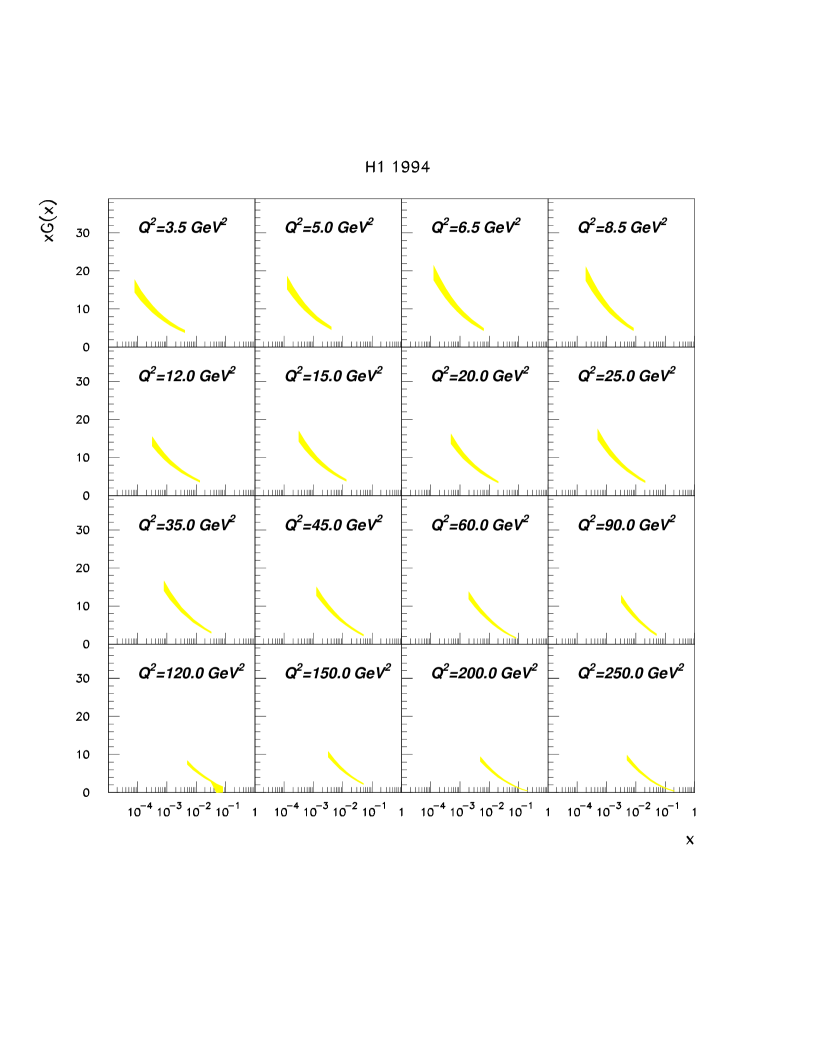
The H1 data [22] has been fitted over the entire $x$ region and for $Q^{2}$ larger than 3.5 $GeV^{2}$. In Fig. 4 we show the results of the fits. We also show the extrapolation from our fits to $Q^{2}$ down to $1.5~{}GeV^{2}$ where the validity of the perturbative expansion is debatable. The gluon density extracted from these fits is presented in Fig. 5 for a restricted $Q^{2}$ range between 3.5 and 250 $GeV^{2}$. One should note that in the first two $Q^{2}$ bins, the predictions tend to be above the data systematically. There could be several reasons for this: missing next to NLO corrections, only two flavours in the proton are excited, or more likely non-perturbative effects, such as higher twist, begin to emerge.

We would like to point out that at very high $Q^{2}$ values, i.e. $Q^{2}\geq 800~{}GeV^{2}$, the phenomenological term $C_{S}(Q^{2})$ which we attribute to the soft pomeron contribution, tends to become small and negative, an effect due to the oversimplified parametrization over the whole $(x,Q^{2})$ range rather than to a genuine physical effect.
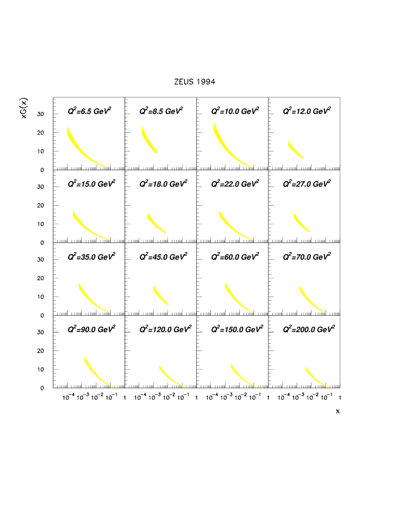
The ZEUS data [23] has been fitted over the entire $x$ range for $Q^{2}$ larger than $6~{}GeV^{2}$. The results of the fits are presented in Fig. 6 up to $Q^{2}=650~{}GeV^{2}$, and the corresponding gluon densities up to $Q^{2}=200~{}GeV^{2}$ in Fig. 7.

Refer to caption

Figure 4: The H1 1994 data along with the results of the fits described in the text

The values of the parameters obtained from fitting the H1 [22] and ZEUS data [23] are summarized in Tables 1 and 2. They are reasonably similar. The $\chi^{2}$ for the fits of the ZEUS data are poorer. The main contribution to the $\chi^{2}$ comes from the high $Q^{2}$ data. Any attempt to fit a smooth function to these data is bound to give poorer $\chi^{2}$ values. We have tried some variations in the fitting procedure by considering the phenomenological term $C_{S}(Q^{2})$ to be proportional to $x^{\epsilon}$, with $\epsilon$ an additional free parameter. The resulting fitted value for $\epsilon$ turned out to be within errors compatible with 00.
We do not expect the parameter $\nu_{0}$ to be well determined by the fits, since it is linked to the behaviour of the structure functions at large $x$ values, while the HERA data are concentrated in the low $x$ domain. A more reliable determination of $\nu_{0}$ would require to incorporate the data from fixed target experiments.

$B_{S}$ $\lambda_{S}$ $A_{S}$ $\nu_{0}$ $\chi^{2}/n.o.p.$
$H1$ $(5.4\pm 0.3)\cdot 10^{-4}$ $0.36\pm 0.01$ $0.46\pm 0.05$ $1.3\pm 0.1$ $162/181$
$ZEUS$ $(4.6\pm 0.3)\cdot 10^{-4}$ $0.35\pm 0.01$ $0.53\pm 0.04$ $1.2\pm 0.1$ $240/175$
Table 1: Summary of the fitted parameters
$B_{S}$ $\lambda_{S}(Q^{2}<10)$ $\lambda_{S}(10<Q^{2}<100)$ $\lambda_{S}(Q^{2}>100)$ $A_{S}$ $\nu_{0}$ $\chi^{2}/n.o.p.$
$H1$ $(4.2\pm 0.3)\cdot 10^{-4}$ $0.33\pm 0.01$ $0.33\pm 0.01$ $0.36\pm 0.01$ $0.40\pm 0.04$ $1.1\pm 0.1$ $112/181$
$ZEUS$ $(3.5\pm 0.3)\cdot 10^{-4}$ $0.32\pm 0.01$ $0.33\pm 0.01$ $0.35\pm 0.01$ $0.42\pm 0.03$ $1.0\pm 0.1$ $202/175$
Table 2: Summary of the fitted parameters

5 Predictions for $R(x,Q^{2})$

As it is well known, in the quark parton model the Callan-Gross relation holds, namely

$$F_{2}(x,Q^{2})=F_{1}(x,Q^{2})$$ (46)

in such a way that the ratio

$$R(x,Q^{2})=\frac{F_{2}(x,Q^{2})-F_{1}(x,Q^{2})}{F_{1}(x,Q^{2})}=\frac{F_{L}(x,Q^{2})}{F_{1}(x,Q^{2})}$$ (47)

vanishes. QCD corrections induce violations of the Callan-Gross rule, leading to non-zero values for $R(x,Q^{2})$. Defining the non-singlet and singlet contributions to $F_{L}$ as

$$F_{L,NS}(x,Q^{2})=\frac{4\alpha_{s}}{3\pi}\int_{x}^{1}dy\frac{x^{2}}{y^{3}}F_{2,NS}(y,Q^{2})$$ (48)

and

$$F_{L,S}(x,Q^{2})=\frac{4\alpha_{s}}{3\pi}\{\int_{x}^{1}dy\frac{x^{2}}{y^{3}}F_{2,S}(y,Q^{2})+\delta_{f}\int_{x}^{1}dy\frac{x^{2}}{y^{3}}(1-\frac{x}{y})F_{G}(y,Q^{2})\}$$ (49)

with

$$\delta_{f}=\frac{3}{2}\cdot n_{f}$$ (50)

and using the parametrizations discussed in previous sections for $F_{S}$ and $F_{G}$, one obtains

$$R(x,Q^{2})=\frac{4\alpha_{s}}{3\pi}\left(\frac{x}{1+\nu(Q^{2})}+\frac{1}{2+\lambda_{S}}\{1~{}+~{}\delta_{f}\cdot\frac{B_{GS}}{3+\lambda_{S}}\cdot(1-x)^{2}\}(1-x)\right)(1-x)$$ (51)

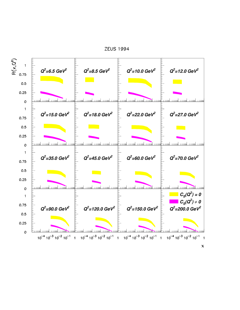
This expression, originally derived in [31] should be valid for large $Q^{2}$ values, where the Pomeron like contribution is negligible. At low and intermediate $Q^{2}$ values, one has to consider the full parametrization for both $F_{S}$ and $F_{G}$, so that one obtains

$\displaystyle R(x,Q^{2})=\frac{4\alpha_{s}}{3\pi}\left(\frac{x}{1+\nu(Q^{2})}+\frac{1}{2+\lambda_{S}}\left\{\frac{B_{S}(Q^{2})\cdot x^{-\lambda_{S}}+\frac{2+\lambda_{S}}{2}\cdot C_{S}(Q^{2})}{B_{S}(Q^{2})\cdot x^{-\lambda_{S}}+C_{S}(Q^{2})}+\right.\right.$ (52)
$\displaystyle\left.\left.\mbox{}+\delta_{f}\cdot\frac{1}{3+\lambda_{S}}\cdot\frac{B_{G}(Q^{2})\cdot x^{-\lambda_{S}}+\frac{(2+\lambda_{S})(3+\lambda_{S})}{6}\cdot C_{G}(Q^{2})}{B_{S}(Q^{2})\cdot x^{-\lambda_{S}}+C_{S}(Q^{2})}(1-x)^{2}\right\}(1-x)\right)(1-x)$

Notice that both expressions are proportional to $\alpha_{s}$. In Fig. 9 we present the predictions from Eq. 52, lower band, derived from the fits to the ZEUS data. The predictions for $R$ exhibit for a given $Q^{2}$ range a smooth rise with decreasing $x$ up to a value of approximately $0.25$. In order to indicate the importance of the Pomeron-like term, we also show the predictions derived from Eq. 51, upper band, which was calculated by setting $C_{S}(Q^{2})=0$. We expect future measurements of $R$ to lie close to the lower values.

6 Conclusions

We have compared recent HERA data on structure functions at low $x$ with QCD analytical calculations. NLO predictions in QCD describe the rate of growth of the proton structure function $F_{2}$ in a wide $Q^{2}$ and $x$ domain. The dominant term behaves like $x^{-\lambda_{S}}$ with $\lambda_{S}\sim 0.34\pm 0.03$ independent of $Q^{2}$. This spread takes into account possible dependences on the number of excited quark flavours. This is in contrast with recent results by the H1 Collaboration which suggested that $\lambda_{S}$ grows from $0.08$ at low $Q^{2}$ to $0.5$ at high $Q^{2}$. We can exclude a BKFL prediction where the exponent $\omega$ in the $x$ behaviour is proportional to the strong coupling constant $\alpha_{s}(Q^{2})$ and therefore decreases with $Q^{2}$.

Acknowledgements

Thanks are due to Drs. C. Glasman, R. Graciani, J. del Peso and J. TerrΓ³n for helpful conversations. We are grateful to G. Wolf for numerous comments and a careful reading of the manuscript.

Refer to caption

Figure 5: The gluon density extracted from the H1 1994 data. The dotted bands indicate the uncertainties in the fitted parameters.

Refer to caption

Figure 6: The ZEUS 1994 data up to $Q^{2}=650~{}GeV^{2}$ along with the results of the fits described in the text.

Refer to caption

Figure 7: The gluon density extracted from the ZEUS 1994 data. The dotted bands indicate the uncertainties in the fitted parameters.

Refer to caption

Figure 8: Predictions for $R(x,Q^{2})$ from fits with $C_{S}(Q^{2})$ equal and non equal to zero, as described in the text. The shaded bands represent the uncertainties in the fitted parameters.

References

  • [1] H1 Coll., T.Β Ahmed et al., Nucl. Phys. B439 (1995) 471Β and I. Abt et al., Nucl. Phys. 407 (1993) 515
  • [2] ZEUS Coll., M.Β Derrick et al., DESY 95-193,Β and Phys. Lett. B316 (1993) 412Β and Z. Phys. C65 (1995) 379
  • [3] ZEUS Coll., M.Β Derrick et al., Phys. Lett. B345 (1995) 576
  • [4] H1 Coll., S.Β Aid et al., Phys. Lett. B354 (1995) 494
  • [5] A.D. Martin, W.J. Sterling and R.G. Roberts, Phys. Lett. B354 (1995) 155, and Phys. Rev. D50 (1994) 6734
  • [6] J. Botts et al., Phys. Lett. B304 (1993) 15
  • [7] M.Glueck, E. Reya and A.Vogt, Phys. Lett. B306 (1993) 391.
  • [8] V.N. Gribov and L.N. Lipatov, Sov. J. Nucl. Phys. 15 (1972) 438,Β G. Altarelli and G. Parisi, Nucl. Phys. B126 (1977) 298
  • [9] E.A. Kuraev et al., JETP 45 (1977) 199 and Y.Y. Balitsky and L.N. Lipatov, Sov. J. Nucl. Phys. 28 (1978) 822
  • [10] A. Β Mueller Nucl. Phys. C18 (191991) 125
  • [11] J. Bartels et al, Z. Phys. C54 (1992) 635Β and K. Kwiecinski et al, Phys. Rev. D46 (1992) 921
  • [12] F.J. YndurΓ‘in, FTUAM-96-12
  • [13] A. de RΓΊjula et al., Phys. Rev. D10 (1974) 1649
  • [14] R.D Ball and S. Forte, Phys. Lett. B335 (1994) 77
  • [15] M. Glueck, E. Reya and M. Stratman Nucl. Phys. B422 (1994) 37
  • [16] S. Riemersma, J. Smith and W.L. van Neerven Phys. Lett. B347 (1994) 77
  • [17] E. Laenen et al., Phys. Lett. B291 (1992) 325
  • [18] E. Witten al., Nucl. Phys. B120 (1977) 189
  • [19] C. LΓ³pez and F.J. YndurΓ‘in, Nucl. Phys. B171 (1980) 231
  • [20] C. LΓ³pez and F.J. YndurΓ‘in, Phys. Rev. Lett. 44 (1980) 1118
  • [21] ZEUS Collaboration, M. Derrick et al., Z. Phys. C69 (1996) 607
  • [22] H1 Collaboration, DESY Preprint 96-039
  • [23] ZEUS Collaboration, M. Derrick et al., DESY preprint 96-76, sub. to Z. Phys.
  • [24] C. LΓ³pez and F.J. YndurΓ‘in, Nucl. Phys. B183 (1981) 157
  • [25] B. Escoubes, M.J. Herrero, C. LΓ³pez and F.J. YndurΓ‘in, Nucl. Phys. B242 (1984) 329
  • [26] F.J. YndurΓ‘in, The theory of quarks and gluons, Springer Verlag.
  • [27] R.K. Ellis, Z. Kunszt and E.M. Levin, Nucl. Phys. B420 (1994) 517
  • [28] A.M. Cooper-Sarkar, R. Devenish and M. Lancaster, Proceedings of the Workshop, Physics at HERA 91, Vol 1 , pag. 155.
  • [29] M. Virchaux and A. Milsztajn, Phys. Lett. B274 (1992) 221
  • [30] W.J. Marciano, Phys. Rev. D29 (1984) 580
  • [31] A. GonzΓ‘lez-Arroyo, C. LΓ³pez and F.J. YndurΓ‘in, Phys. Lett. B98 (1981) 215