TUM–HEP–241/96

MPI–PhT/96–21

Gauge Coupling Unification in Left–Right
 
Symmetric Models

M. Lindner and M. Weiser

Institut für Theoretische Physik, Technische Universität München,

James–Franck–Strasse, D–85748 Garching, GERMANY

Abstract

We explore possibilities of gauge coupling unification in left–right symmetric models with non–minimal particle content. In addition to unification we require the absence of anomalies and sufficient proton lifetime. Numerous previously unknown solutions are presented where unification occurs within the latest experimental errors. Solutions exist where the scale of left–right symmetry breaking can be as low as ${\cal O}(TeV)$ or the scale $M_{GUT}$ as high as the Planck scale.

Work supported in part by EC grant ERB SC1*CT000729 and DFG grant Li519/2–1

It is well known that gauge coupling unification is possible in the minimal left–right (LR) symmetric model [1] if the scale of LR symmetry breaking, $M_{R}$, is chosen around $10^{10}$ GeV (see e.g., [2]). Attempts to lower or rise $M_{R}$ sizably require a different, non–minimal particle content. Two possible directions for such changes which modify the $\beta$–functions (and thus gauge coupling unification) are: (i) supersymmetrization or (ii) new (“exotic”) fermionic and/or scalar representations. In the supersymmetric case a few solutions for gauge coupling unification with low $M_{R}$ are already known. Deshpande, Keith and Rizzo [3] investigated for example a SUSY–$SO(10)$ scenario (which is supersymmetric both in the LR and the Standard Model sector) and found at two–loop level unification for $M_{R}=1$ TeV at the scale $M_{X}\approx 10^{16.2\pm 0.4}$ GeV. They also studied non–supersymmetric $SO(10)$–unification and concluded that one would need a large number of Higgs doublets and triplets coming from the scalar representations 16 and 126, respectively. In addition, $M_{GUT}=10^{13.6}$ GeV would be much too low. Two further solutions were recently presented by Ma, where the supersymmetric LR model is embedded into a larger supersymmetric gauge group: In one case [4] into the SUSY–$SO(10)$ (with additional discrete symmetries) and SUSY–$SO(10)\otimes SO(10)$, respectively, and in the other case [5] into the SUSY–$E6$. In both cases, however, new exotic fermions must be postulated in order to achieve gauge coupling unification for a low right–handed scale. We will discuss in this letter interesting solutions which emerge from new fermionic and scalar particles in left–right symmetric models even without supersymmetry. To our knowledge viable scenarios which achieve unification even with $M_{R}={\cal O}(TeV)$ in non–supersymmetric left–right models were not published so far.

Let us recall some attempts to modify the original minimal $SU(5)$ embedding of the Standard Model where the proton life time, $\tau_{P}$, and the weak mixing angle, $sin^{2}(\theta_{W})$, are too small. Frampton and Glashow [7] proposed originally to add a few chiral fermion multiplets in real representations with the same quantum numbers as the known quarks and leptons. In this way it was possible to increase $\tau_{P}$ and $\sin^{2}(\theta_{W})$ by the necessary amounts. When more precise data became available Amaldi, de Boer, Frampton, Fürstenau, and Liu [9] repeated the analysis of the gauge coupling unification [8] for the Standard Model, the minimal supersymmetric Standard Model and an adequately modified $SU(5)$ with exotic fermions and extra scalars. They investigated the running of gauge couplings for different combinations of new multiplets at the two–loop level where the contribution of exotic particles started at a common effective mass scale. This threshold scale was treated as a free parameter in the range of $M_{Z}\leq M_{thres}\leq 10$ TeV. In this way they were able to find many unification solutions, even if they added only four multiplets. In all of these cases there is no contradiction with proton life time, and by using only real representations potential chiral anomalies are automatically avoided.

Our aim is to perform a similar search for gauge coupling unification in the class of left–right symmetric models. We will therefore extend the minimal LR model and introduce new fermionic and scalar multiplets which we call “exotic”. The effects of these particles will be switched on at a common effective threshold which is essentially identical to the right handed scale $M_{R}$. We calculate the relevant $\beta$–functions to one–loop order and restrict ourselves to cases where this is sufficient. We search only for gauge unification solutions with no specific GUT–scenario in mind. Therefore we pay no attention to whether these representations fit into representations of a specific GUT group. The requirements for a “solution” are unification within the current $1\sigma$–error bars of inverse couplings and sufficient proton life time. Furthermore we require the absence of Landau poles before unification. Since we do not restrict our search to real representations we must also pay attention to potential anomalies.

This letter is organized as follows: First we introduce the notation and simultaneously remind the reader about some features of the minimal LR model. Next the anomaly coefficients and the $\beta$–function contributions are determined for different new “exotic” particles and listed in tables. Finally we search for solutions with the mentioned requirements and present numerous previously unknown solutions for unification in non–minimal and non–supersymmetric left–right models.

We study left–right symmetric extensions of the Standard Model with the gauge group $G=SU(3)_{c}\otimes SU(2)_{L}\otimes SU(2)_{R}\otimes U(1)_{B-L}$. Representations of this gauge group are written as $(N_{c},N_{L},N_{R},B-L)_{l,r}$, where $N_{c}$, $N_{L}$, $N_{R}$ are the dimensions under $SU(3)_{c}$, $SU(2)_{L}$ and $SU(2)_{R}$, respectively, where $B-L$ is the $U(1)_{B-L}$ quantum number, and where the index “l” or “r” specifies the chirality in case of fermionic representations. Since we deal with non–minimal scenarios it is important to remember that the indices “L” and “R” of the $SU(2)$ groups are not necessarily related to the chiralities “l” and “r” of the fermions. In the Standard Model and in the minimal left–right symmetric model the chiralities “l” and “r” are uniquely related to one of the $SU(2)$ groups thus justifying to speak of “left” and “right” gauge groups. In general, however, a direct connection between the chiralities of the fermions and their quantum numbers is not required. We are thus free to choose the chirality of any additional non–standard fermion representation of the gauge group. In this way it is possible to introduce, for example, bi–doublet fermions. Obviously “$B-L$” is also no longer related to baryon and lepton number for such exotic particles and we will therefore write “$B-L+X$” where appropriate. We postulate however a generalized discrete left–right symmetry, which requires a representation content which is symmetric under the simultaneous exchange of “L” $\leftrightarrow$ “R” and the chiralities “l” $\leftrightarrow$ “r”. This generalization of discrete left–right symmetry becomes necessary when the connection between the gauge groups and chiralities is not present. Discrete left–right symmetry enforces as usual that the $SU(2)$ gauge couplings are identical: $g_{2L}\equiv g_{2R}\equiv g_{2}$.

The so–called minimal left–right symmetric model contains a remarkable simple set of possible irreducible representations. The gauge bosons are $G^{c}_{\mu}$, $W^{i}_{L\mu}$, $W^{i}_{R\mu}$, $B_{\mu}$ for $SU(3)_{c}$, $SU(2)_{L}$, $SU(2)_{R}$, $U(1)_{B-L}$, respectively. The three known generations of quarks and leptons fit very economically into the discrete left–right symmetric set of representations $Q_{L}\sim(3,2,1,1/3)_{l}$, $Q_{R}\sim(3,1,2,1/3)_{r}$, $\Psi_{L}\sim(1,2,1,-1)_{l}$ and $\Psi_{R}\sim(1,1,2,-1)_{r}$, or more explicitly:

$$\begin{array}[]{ccc}Q_{L/R}={u_{c}\choose d_{c}}_{l/r}~{},&{c_{c}\choose s_{c}}_{l/r}~{},&{t_{c}\choose b_{c}}_{l/r}~{},\\ \\ \Psi_{L/R}={\nu_{e}\choose e^{-}}_{l/r}~{},&{\nu_{\mu}\choose\mu^{-}}_{l/r}~{},&{\nu_{\tau}\choose\tau^{-}}_{l/r}~{}.\end{array}$$ (1)

The Higgs sector contains finally the scalar bi–doublet

$$\Phi\cong\left(\begin{array}[]{cc}\Phi_{1}^{0}&\Phi_{1}^{+}\\ \Phi_{2}^{-}&\Phi_{2}^{0}\end{array}\right)~{},$$ (2)

with $\Phi\sim(1,2,2,0)$ and two scalar triplets $\Delta_{L}$, $\Delta_{R}\sim(1,3,1,2)\oplus(1,1,3,2)$. Any left–right model with a larger or modified particle content will be called non–minimal.

We will consider new exotic fermions which can give rise to chiral anomalies. We consider therefore only anomaly free combinations. The individual triangle anomaly contributions are proportional to

$$A^{abc}:=\frac{1}{2}Tr\left[\{T^{a},T^{b}\}T^{c}\right]~{}.$$ (3)

Here $T^{a}$ are the generators of the fermion representations which act at the vertices. For abelian groups (as the $U(1)$ is) $T^{a}$ is just a multiple of the unity matrix. If $A^{abc}$ vanishes for all indices $a$, $b$, and $c$ then all higher order anomalies are absent, too. If the fermions are given in a chiral basis with left– and right–handed states, $A^{abc}$ can be written as [10]

$$A^{abc}=2\cdot\left(A_{l}^{abc}-A_{r}^{abc}\right)~{},$$ (4)

where

$$A_{l,r}^{abc}:=\frac{1}{2}Tr\left[\{T_{l,r}^{a},T_{l,r}^{b}\}T_{l,r}^{c}\right]~{}.$$ (5)

Here $T_{l}^{a}$ and $T_{r}^{a}$ are the generators of the representations of the left–handed and right–handed fermions, respectively.

Choi and Volkas [11] studied chiral anomalies which arise from exotic fermions in left–right symmetric models. They showed that all chiral anomalies except those of the type $[SU(2)_{L}]^{2}[U(1)_{B-L}]$ and $[SU(2)_{R}]^{2}[U(1)_{B-L}]$ cancel if the following two conditions are fulfilled:

• The number of left–handed fermionic representations $(N_{c},N_{L},N_{R},B-L+X)_{l}$ is equal to the number of the corresponding right–handed representations
  $(N_{c},N_{R},N_{L},B-L+X)_{r}$.

• The $U(1)$ quantum numbers of both representations are equal.

Note that these conditions are automatically fulfilled in our case since they are equivalent to the generalized discrete left–right symmetry. Eventually surviving $[SU(2)_{L}]^{2}[U(1)_{B-L}]$ and $[SU(2)_{R}]^{2}[U(1)_{B-L}]$ anomalies can be calculated by a simple formula which reads in our notation

$$A_{L,l}^{abc}\left((N_{c},N_{L},N_{R},b)_{l}\right) = N_{c}\cdot c_{2}(T_{l}^{(N_{L}-dim.)})\cdot N_{R}\cdot b~{},$$ (6)

$$A_{L,r}^{abc}\left((N_{c},N_{L},N_{R},b)_{r}\right) = N_{c}\cdot c_{2}(T_{r}^{(N_{L}-dim.)})\cdot N_{R}\cdot b~{}.$$ (7)

Here $A_{L}^{abc}$ and $A_{R}^{abc}$ are the triangle anomaly coefficients of the type $[SU(2)_{L}]^{2}[U(1)_{B-L}]$ and $[SU(2)_{R}]^{2}[U(1)_{B-L}]$. For left–handed (right–handed) representations $(N_{c},N_{L},N_{R},b)_{l}$ ( $(N_{c},N_{L},N_{R},b)_{r}$ ) the anomaly coefficients are called $A_{L,l}^{abc}$ and $A_{R,l}^{abc}$ ($A_{L,r}^{abc}$ and $A_{R,r}^{abc}$). $T_{l/r}^{(N_{L}-dim.)}$ is a $N_{L}$-dimensional representation of $SU(2)_{L}$, and $c_{2}$ is its “index” which we will define and discuss later on in the context of the $\beta$–functions. For a singlet we have $c_{2}(1)=0$. The coefficients $A_{R,l}^{abc}$ and $A_{R,r}^{abc}$ can be easily obtained via

$$A_{R,l}^{abc}\left((N_{c},N_{L},N_{R},b)_{l}\right) = A_{L,l}^{abc}\left((N_{c},N_{R},N_{L},b)_{l}\right)~{},$$ (8)

$$A_{R,r}^{abc}\left((N_{c},N_{L},N_{R},b)_{r}\right) = A_{L,r}^{abc}\left((N_{c},N_{R},N_{L},b)_{r}\right)~{}.$$ (9)

Equation (4) can now be rewritten as

$$A_{L} = 2\cdot\left(A_{L,l}-A_{L,r}\right)~{},$$ (10)

$$A_{R} = 2\cdot\left(A_{R,l}-A_{R,r}\right)~{}.$$ (11)

The contributions to $A_{L}$ and $A_{R}$ are calculated for a number of representations and are listed later in Table 3 together with their contributions to the $\beta$–functions. This will allow us to search for anomaly free combinations of exotic fermions.

The unification of running gauge couplings in the presence of exotic particles has been studied in supersymmetric extensions of the left–right model. In the literature are, however, only a few attempts of such studies which extend the minimal left–right symmetric model by some “exotic” particles like higher–dimensional (not fundamental) irreducible representations. A search for anomalies in left–right models was performed by Choi and Volkas [11]. We use some of their results and combine it with a search for unification solutions.

The evolution of the gauge couplings $g_{i}$, $i=1,2,3$ is (for a given model with known particle content) governed by the corresponding $\beta$–functions

$$\mbox{$\displaystyle\frac{dg_{i}(t)}{dt}$}=\beta_{g_{i}}(g_{j}(t))~{},$$ (12)

where the dimensionless scale parameter is as usually defined through $t:=\ln\left(\frac{\mu}{\mu_{0}}\right)$. To one–loop order $\beta_{g_{i}}$ has the form

$$\beta_{g_{i}}=\frac{(g_{i})^{3}}{16\pi^{2}}\cdot b_{i}~{},$$ (13)

where $b_{i}$ is constant over some (or the whole) energy range. Since we consider only weak couplings we can restrict ourselves to one–loop calculations. Particle thresholds are described in first approximation by the $\theta$–function approach with the assumption that the new particles we introduce are not too wide spread around the common scale $M_{R}$ which denotes the effective mass scale of the left–right symmetric model. For the one–loop beta functions we use the following general form given by Jones [12]:

$$\beta_{g} = \frac{(g)^{3}}{16\pi^{2}}\cdot\left[~{}-\frac{11}{3}c_{1}+\frac{2}{3}\sum_{R_{f}}c_{2}(R_{f})\cdot d_{1}(R_{f})\cdot\dots\cdot d_{n}(R_{f})\right.$$ (14)

$$\left.+\frac{1}{3}~{}\sum_{R_{s}}c_{2}(R_{s})\cdot d_{1}(R_{s})\cdot\dots\cdot d_{n}(R_{s})~{}\right]~{}.$$

The meaning of the notation is as follows: For a given group factor $G_{0}$ we can write the full gauge group $G$ as a direct product in the form

$$G=G_{0}\otimes X_{1}\otimes\dots\otimes X_{n}~{},$$ (15)

where $g$ is the coupling which belongs to $G_{0}$. $R_{f}$ is then any irreducible chiral representation of fermions and $R_{s}$ is any irreducible scalar representation of $G_{0}$. $d_{i}(R)$ is the dimension of the representation $R$ under the group factor $X_{i}$. The constants $c_{2}(R)$ are fixed by the choice of representations and depend on their dimensions. They are defined through

$$c_{2}(R)\cdot\delta^{ab}:=Tr[R^{a}R^{b}]~{},$$ (16)

and are equivalent to a normalization of the generators of $R$. $c_{2}(R)$ is called the “index” of the irreducible representation $R$ and is often also denoted by $T(R)$. Furthermore we have as usual $c_{1}=c_{2}(R^{adj})$ ($=N$ for $SU(N)$).

With eq. (14) the calculation of $\beta$–functions is reduced to the task of finding $c_{2}(R)$ for the relevant representations. In our convention we have $Tr[R^{a}R^{b}]=\frac{1}{2}\delta^{ab}$ and $c_{2}$ can be determined for any representation with the help of the so–called “Dynkin–labels” [13, 14]. Note that the values given in refs. [13, 14] differ by normalization conventions, in the case of ref. [13] a factor 2 and in the case of ref. [14] a factor $2\cdot rank(G)$. In Tables 2 and 2 we list some values of $c_{2}$ which we will use.

Dynkin–Label	Representation	$c_{2}$
(1)	2	$\frac{\textstyle 1}{\textstyle 2}$
(2)	3	2
(3)	4	5
(4)	5	10
(5)	6	$\frac{\textstyle 35}{\textstyle 2}$
(6)	7	28
(7)	8	42
(8)	9	60
(9)	10	$\frac{\textstyle 165}{\textstyle 2}$
(10)	11	110

Table 1: $c_{2}(R)$ for some irreducible representations of $SU(2)$

Dynkin–Label	Representation	$c_{2}$
(1,0)	3	$\frac{\textstyle 1}{\textstyle 2}$
(2,0)	6	$\frac{\textstyle 5}{\textstyle 2}$
(1,1)	8	3
(3,0)	10	$\frac{\textstyle 15}{\textstyle 2}$
(2,1)	15	10
(4,0)	15	$\frac{\textstyle 35}{\textstyle 2}$
(0,5)	21	35
(1,3)	24	25
(2,2)	27	27
(6,0)	28	63

Table 2: $c_{2}(R)$ for some irreducible representations of $SU(3)$

With this information it is easy to confirm for example the coefficients $b_{i}$ of the one–loop $\beta$–functions of the minimal left–right symmetric model to be

$$\left(\begin{array}[]{c}b_{1}\\ b_{2}\\ b_{3}\end{array}\right)_{\bf LR}=\left(\begin{array}[]{c}0\\ -\frac{22}{3}\\ -11\end{array}\right)+N_{G}\cdot\left(\begin{array}[]{c}\frac{4}{3}\\ \frac{4}{3}\\ \frac{4}{3}\end{array}\right)+N_{HBiD}\cdot\left(\begin{array}[]{c}0\\ \frac{1}{3}\\ 0\end{array}\right)+N_{HTr}\cdot\left(\begin{array}[]{c}3\\ \frac{2}{3}\\ 0\end{array}\right)~{},$$ (18)

where $N_{G}=3$ is the number of (complete) fermion generations, $N_{HBiD}=1$ is the number of Higgs bidoublets, and $N_{HTr}=1$ is the number of pairs of Higgs triplets. These coefficients will be modified if we introduce some new (exotic) particles. We list therefore in Table 3 contributions of exotic fermion representations to the $\beta$–functions (together with the chiral anomaly contributions $A_{L}$ and $A_{R}$ discussed above). Furthermore we list in Table 4 a number of scalar representations and their contributions to the $\beta$–functions.

Irreducible representation	Contribution	Anomaly coefficient
$(3_{c},2_{L},2_{R},B-L+X)_{l,r}$	$(b_{1},b_{2},b_{3})$		$A_{L}$			$A_{R}$
$(1,1,1,b)_{l}\oplus(1,1,1,b)_{r}$	($\frac{\textstyle 1}{\textstyle 2}b^{2}$, 0, 0)		0			0
$(3,1,1,b)_{l}\oplus(3,1,1,b)_{r}$	($\frac{\textstyle 3}{\textstyle 2}b^{2}$, 0, $\frac{\textstyle 4}{\textstyle 3}$)		0			0
$(6,1,1,b)_{l}\oplus(6,1,1,b)_{r}$	($3b^{2}$, 0, $\frac{\textstyle 20}{\textstyle 3}$)		0			0
$(8,1,1,b)_{l}\oplus(8,1,1,b)_{r}$	($4b^{2}$, 0, 8)		0			0
$(10,1,1,b)_{l}\oplus(10,1,1,b)_{r}$	($5b^{2}$, 0, 20)		0			0
$(1,2,1,-1)_{l}\oplus(1,1,2,-1)_{r}$	(1, $\frac{\textstyle 1}{\textstyle 3}$, 0)	l: -1		r: 0	l: 0		r: 1
$(1,2,1,b)_{l}\oplus(1,1,2,b)_{r}$	($b^{2}$, $\frac{\textstyle 1}{\textstyle 3}$, 0)	l: b		r: 0	l: 0		r: -b
$(1,2,2,b)_{l}\oplus(1,2,2,b)_{r}$	($2b^{2}$, $\frac{\textstyle 2}{\textstyle 3}$, 0)		0			0
$(1,3,1,b)_{l}\oplus(1,1,3,b)_{r}$	($\frac{\textstyle 3}{\textstyle 2}b^{2}$, $\frac{\textstyle 4}{\textstyle 3}$, 0)	l: 4b		r: 0	l: 0		r: -4b
$(1,3,2,b)_{l}\oplus(1,2,3,b)_{r}$	($3b^{2}$, $\frac{\textstyle 8}{\textstyle 3}$, 0)	l: 8b		r: -3b	l: 3 b		r: -8b
$(1,3,3,b)_{l}\oplus(1,3,3,b)_{r}$	($\frac{\textstyle 9}{\textstyle 2}b^{2}$, 4, 0)		0			0
$(3,2,1,\frac{1}{3})_{l}\oplus(3,1,2,\frac{1}{3})_{r}$	($\frac{\textstyle 1}{\textstyle 3}$, 1, $\frac{\textstyle 4}{\textstyle 3}$)	l: 1		r: 0	l: 0		r: -1
$(3,2,1,b)_{l}\oplus(3,1,2,b)_{r}$	($3b^{2}$, 1, $\frac{\textstyle 4}{\textstyle 3}$)	l: 3b		r: 0	l: 0		r: -3b
$(3,2,2,b)_{l}\oplus(3,2,2,b)_{r}$	($6b^{2}$, 2, $\frac{\textstyle 8}{\textstyle 3}$)		0			0
$(3,3,1,b)_{l}\oplus(3,1,3,b)_{r}$	($\frac{\textstyle 9}{\textstyle 2}b^{2}$, 4, 2)	l: 12b		r: 0	l: 0		r: -12b
$(3,3,2,b)_{l}\oplus(3,2,3,b)_{r}$	($9b^{2}$, 8, 4)	l: 24b		r: -9b	l: 9b		r: -24b
$(3,3,3,b)_{l}\oplus(3,3,3,b)_{r}$	($\frac{\textstyle 27}{\textstyle 2}b^{2}$, 12, 6)		0			0

Table 3: Contributions of fermion representations to the $\beta$–functions and anomaly coefficients. The assignments of chirality “l” and “r” are essentially arbitrary. The symbol “$\oplus$” denotes a pair of representations respecting the generalized discrete left–right symmetry. The $B-L+X$ charge $b$ can take different values for different pairs of representations; i.e., in general the $b$’s differ from line to line.

Irreducible representation	Contribution to
$(3_{c},2_{L},2_{R},B-L+X)$	$(b_{1},b_{2},b_{3})$
$(1,1,1,b)$	($\frac{\textstyle 1}{\textstyle 8}b^{2}$, 0, 0)
$(1,2,1,1)\oplus(1,1,2,1)$	($\frac{\textstyle 1}{\textstyle 2}$, $\frac{\textstyle 1}{\textstyle 6}$, 0)
$(1,2,1,b)\oplus(1,1,2,b)$	($\frac{\textstyle 1}{\textstyle 2}b^{2}$, $\frac{\textstyle 1}{\textstyle 6}$, 0)
$(1,2,2,0)$	(0, $\frac{\textstyle 1}{\textstyle 3}$, 0)
$(1,2,2,b)$	($\frac{\textstyle 1}{\textstyle 2}b^{2}$, $\frac{\textstyle 1}{\textstyle 3}$, 0)
$(1,3,1,2)\oplus(1,1,3,2)$	(3, $\frac{\textstyle 2}{\textstyle 3}$, 0)
$(1,3,1,b)\oplus(1,1,3,b)$	($\frac{\textstyle 3}{\textstyle 4}b^{2}$, $\frac{\textstyle 2}{\textstyle 3}$, 0)
$(1,3,2,b)\oplus(1,2,3,b)$	($\frac{\textstyle 3}{\textstyle 2}b^{2}$, $\frac{\textstyle 4}{\textstyle 3}$, 0)
$(1,3,3,b)$	($\frac{\textstyle 9}{\textstyle 8}b^{2}$, 2, 0)
$(3,1,1,b)$	($\frac{\textstyle 3}{\textstyle 8}b^{2}$, 0, $\frac{\textstyle 1}{\textstyle 6}$)
$(6,1,1,b)$	($\frac{\textstyle 3}{\textstyle 4}b^{2}$, 0, $\frac{\textstyle 5}{\textstyle 6}$)
$(8,1,1,b)$	($b^{2}$, 0, 1)
$(3,2,1,b)\oplus(3,1,2,b)$	($\frac{\textstyle 3}{\textstyle 2}b^{2}$, $\frac{\textstyle 1}{\textstyle 2}$, $\frac{\textstyle 2}{\textstyle 3}$)
$(3,2,2,b)$	($\frac{\textstyle 3}{\textstyle 2}b^{2}$, 1, $\frac{\textstyle 2}{\textstyle 3}$)

Table 4: Contributions of some scalar representations to the $\beta$–functions.

$F_{1}$	$F_{2}$	$F_{3}$	$H_{1}$	$H_{2}$	$H_{3}$	$M_{R}$ [GeV]	$M_{GUT}$ [GeV]	$\alpha_{GUT}^{-1}$	$\tau_{P}$ [yrs]
0	0	1 (1)	0	1	1	$2\cdot 10^{3}$	$10^{16.6}$	33.1	$7.9\cdot 10^{37}$
0	0	1 (1)	0	1	2	$1\cdot 10^{3}$	$10^{14.7}$	29.7	$1.6\cdot 10^{30}*$
0	0	1 (1)	0	2	1	$1\cdot 10^{6}$	$10^{15.9}$	34.6	$1.3\cdot 10^{35}$
0	0	1 (1)	1	1	0	$2\cdot 10^{4}$	$10^{18.3}$	36.9	$6.2\cdot 10^{44}$
0	0	1 (1)	1	1	1	$5\cdot 10^{3}$	$10^{16.1}$	32.7	$7.7\cdot 10^{35}$
0	0	1 (1)	1	2	0	$5\cdot 10^{6}$	$10^{17.2}$	37.3	$2.5\cdot 10^{41}$
0	0	1 (1)	2	1	0	$5\cdot 10^{4}$	$10^{17.7}$	36.2	$2.4\cdot 10^{42}$
0	0	2 ($\frac{\textstyle 2}{\textstyle 3}$)	0	1	1	$4\cdot 10^{4}$	$10^{19}$	24.1	$1.7\cdot 10^{47}$
0	1 ($\frac{\textstyle 5}{\textstyle 3}$)	0	1	1	0	$2\cdot 10^{8}$	$10^{15.3}$	42.8	$8.4\cdot 10^{32}*$
0	1 ($\frac{\textstyle 2}{\textstyle 3}$)	1 (1)	0	1	1	$4\cdot 10^{6}$	$10^{15.2}$	34.2	$2.1\cdot 10^{32}*$
0	1 ($\frac{\textstyle 4}{\textstyle 3}$)	1 ($\frac{\textstyle 2}{\textstyle 3}$)	1	1	0	$1\cdot 10^{8}$	$10^{16.4}$	37.4	$1.6\cdot 10^{37}$
1 ($\frac{\textstyle 5}{\textstyle 3}$)	0	0	0	1	1	$1\cdot 10^{3}$	$10^{16.5}$	42.7	$5.3\cdot 10^{37}$
1 ($\frac{\textstyle 5}{\textstyle 3}$)	0	0	0	1	2	$1\cdot 10^{3}$	$10^{14.5}$	38.1	$4.2\cdot 10^{29}*$
1 ($\frac{\textstyle 5}{\textstyle 3}$)	0	0	0	2	1	$4\cdot 10^{5}$	$10^{15.9}$	41.6	$1.1\cdot 10^{35}$
1 ($\frac{\textstyle 5}{\textstyle 3}$)	0	0	1	1	0	$6\cdot 10^{3}$	$10^{18.4}$	47.2	$2.6\cdot 10^{45}$
1 ($\frac{\textstyle 5}{\textstyle 3}$)	0	0	1	1	1	$3\cdot 10^{3}$	$10^{16}$	41.6	$5.0\cdot 10^{35}$
1 (2)	0	0	1	2	0	$1\cdot 10^{3}$	$10^{17}$	43.9	$5.6\cdot 10^{39}$
1 ($\frac{\textstyle 5}{\textstyle 3}$)	0	0	2	1	0	$2\cdot 10^{4}$	$10^{17.7}$	45.7	$3.8\cdot 10^{42}$
1 ($\frac{\textstyle 2}{\textstyle 3}$)	0	1 ($\frac{\textstyle 2}{\textstyle 3}$)	0	1	1	$4\cdot 10^{4}$	$10^{19}$	34.7	$3.5\cdot 10^{47}$
1 ($\frac{\textstyle 4}{\textstyle 3}$)	1 ($\frac{\textstyle 4}{\textstyle 3}$)	0	0	1	1	$5\cdot 10^{4}$	$10^{14.9}$	39.3	$1.8\cdot 10^{31}*$
1 ($\frac{\textstyle 4}{\textstyle 3}$)	1 ($\frac{\textstyle 4}{\textstyle 3}$)	0	1	1	0	$2\cdot 10^{5}$	$10^{16.2}$	42.4	$3.3\cdot 10^{36}$
2 ($\frac{\textstyle 1}{\textstyle 3}$)	0	0	0	1	1	$4\cdot 10^{6}$	$10^{18.7}$	45.6	$3.8\cdot 10^{46}$

Table 5: Unification solutions with less or equal 4 extra representations. $F_{1}$, $F_{2}$, $F_{3}$ and $H_{1}$, $H_{2}$, $H_{3}$ are the numbers of fermions and scalars mentioned in the text. $F_{4}$ and $F_{5}$ are here always zero. The numbers in brackets in the fermionic columns are the $U(1)$ charges. The table lists the LR–scale $M_{R}$, the GUT scale $M_{GUT}$, the inverse coupling at $M_{GUT}$ and the proton life time. A ‘$*$’ after $\tau_{P}$ marks cases which are close to the proton decay limit.

We have now all necessary ingredients to search for anomaly free combinations of exotic particles which lead to left–right gauge unification. We define $\alpha_{i}=g_{i}^{2}/4\pi$ and evolve $\alpha_{i}^{-1}$ which becomes simply

$$\frac{d\alpha_{i}^{-1}}{dt}=-~{}\frac{b_{i}}{2\pi}~{}.$$ (19)

In a first step the Standard Model is evolved with its known particle content to a common left–right scale $M_{R}$ where the left–right evolution starts. Eq. (14) allows us to determine the well known $\beta$–function coefficients for the Standard Model (with $N_{G}=3$ and with the $U(1)_{Y}$ coupling in GUT–normalization, i.e. multiplied by a factor $3/5$)

$$\left(\begin{array}[]{c}b_{1Y}\\ b_{2}\\ b_{3}\end{array}\right)_{\bf SM}=\left(\begin{array}[]{c}+\frac{41}{10}\\ -\frac{19}{6}\\ -7\end{array}\right)~{}.$$ (20)

The experimental initial values for the gauge couplings at $M_{Z}$ are taken to be:

$$\left(\begin{array}[]{c}\alpha_{1Y}^{-1}(M_{Z})\\ \alpha_{2}^{-1}(M_{Z})\\ \alpha_{3}^{-1}(M_{Z})\end{array}\right)=\left(\begin{array}[]{c}59.41\pm 0.08\\ 29.88\pm 0.06\\ \ 8.55\pm 0.51\end{array}\right)~{}.$$ (21)

Beyond $M_{R}$ we continue to run the gauge couplings in a next step with the left–right model for an arbitrary (but anomaly free) particle content to the GUT–scale $M_{GUT}$. However, the different normalizations of the $U(1)$ generators must be taken into account: $\alpha_{1}^{-1}\equiv\alpha_{1,B-L}^{-1}=\frac{5}{2}\alpha_{1Y}^{-1}-\frac{3}{2}\alpha_{2}^{-1}$. For the evolution of the left–right model we need the coefficients $b_{i}$ which receive contributions from all particles. First there are the contributions from all the gauge fields which are indisputable. Next we always add the contributions of the known fermions. Since the gauge fields are already included it is obvious that any further contribution to $b_{i}$ must be positive. Thus we obtain lower bounds for the coefficients $b_{i}$ if we just include the gauge field and the known fermion contributions:

$$\left(\begin{array}[]{c}b_{1,min}\\ b_{2,min}\\ b_{3,min}\end{array}\right)_{\bf LR}=\left(\begin{array}[]{c}4\\ -\frac{10}{3}\\ -7\end{array}\right)~{}.$$ (22)

There exist also upper bounds on $b_{i}$ in order to avoid Landau poles in the gauge couplings before the unification scale $M_{GUT}$ is reached. From the evolution equation (19) follows that for large enough $b_{i}$ the inverse coupling $\alpha_{i}^{-1}$ will run to zero before the GUT–scale is reached. In order to avoid such Landau singularities the coefficients $b_{i}$ must be limited from above:

$$b_{i}\leq b_{i,max}=\frac{2\pi\alpha_{i}^{-1}(M_{R})}{\ln(M_{GUT}/M_{R})}~{}.$$ (23)

With $M_{R}=1$ TeV, $10^{19}$ GeV $=M_{Planck}\geq M_{GUT}\geq 10^{15}$ GeV and the initial values eq. (21) one finds for example

$$\left(\begin{array}[]{c}b_{1,max}\\ b_{2,max}\\ b_{3,max}\end{array}\right)_{\bf LR}\raisebox{-1.72218pt}{\hbox to0.0pt{$\sim$\hss}}\raisebox{1.72218pt}{$<$}\left(\begin{array}[]{c}20.55\\ 6.89\\ 2.55\end{array}\right)~{}.$$ (24)

There exist also severe restrictions on the differences $b_{3}-b_{2}$ and $b_{3}-b_{1}$ which come from the requirement of unification of $\alpha_{3}$ with $\alpha_{2}$ and $\alpha_{3}$ with $\alpha_{1}$ in an acceptable scale range. First, for phenomenological reasons, we must require $1$ TeV $\leq M_{R}\leq M_{GUT}$. The GUT–scale itself should lie below the Planck–scale $M_{Planck}=10^{19}$ GeV. An additional strong lower bound for potential GUT–scales comes from the proton lifetime. We do not discuss here any specific GUT model, but simply demand that the GUT–scale is high enough to avoid such problems. The proton life time is parameterized in terms of the usual relation

$$\tau_{proton}\approx\frac{1}{(\alpha_{GUT})^{2}}\cdot\frac{M_{GUT}^{4}}{M_{proton}^{5}}~{},$$ (25)

derived from an effective low energy four–fermion approximation for the decay channel $p\rightarrow e^{+}+\pi^{0}$. For all potential GUT scenarios with exotic particles we require that the experimental lower bound [18] $\tau_{P}/B(p\rightarrow e^{+}+\pi^{0})>9\cdot 10^{32}~{}y$ is not badly violated. To fulfill this we demand $M_{GUT}\geq 10^{15}$ GeV in our search. Solutions which lead to $M_{GUT}$ close to this lower bound should be carefully checked if they lead to problems with proton decay. In principle such a check should include the discussion of decay modes, threshold corrections and higher orders in the $\beta$–functions. From the above requirements on the involved scales one finds severe restrictions on $b_{3}-b_{2}$ and $b_{3}-b_{1}$. For $M_{R}=1$ TeV one finds for example $-4.33\leq b_{3}-b_{2}\leq-3.25$ and $-20\leq b_{3}-b_{1}\leq-15$.

The above constraints on the coefficients $b_{i}$ lead to restrictions on the possible representation content of GUT solutions. Since larger representations contribute via eq. (14) systematically more to the beta functions we can derive the largest representation which does not lead to a Landau pole. This largest representation is given by the requirement that the additional contributions to $b_{i}$ are smaller than $b_{i,max}-b_{i,min}$. So we must exclude from Table 3 the entries $(10,1,1,b)_{l}\oplus(10,1,1,b)_{r}$ and $(3,3,3,b)_{l}\oplus(3,3,3,b)_{r}$ since the limits for $b_{2}$ and $b_{3}$, respectively, are exceeded. We further exclude $(6,1,1,b)_{l}\oplus(6,1,1,b)_{r}$, $(8,1,1,b)_{l}\oplus(8,1,1,b)_{r}$, and $(3,3,2,b)_{l}\oplus(3,2,3,b)_{r}$, even though the limits in $b_{2}$ and $b_{3}$ are not yet reached. It would however be impossible to add any other fermionic representations which would respect these limits and the one of $b_{3}-b_{2}$ and lead to unification. Some of the remaining representations should occur only in “natural”, anomaly free combinations, namely $(1,2,1,b_{a})_{l}\oplus(1,1,2,b_{a})_{r}$ together with $(3,2,1,b_{b})_{l}\oplus(3,1,2,b_{b})_{r}$, which is a slight variation of one standard fermion generation, and $(1,3,1,b_{c})_{l}\oplus(1,1,3,b_{c})_{r}$ together with $(3,3,1,b_{d})_{l}\oplus(3,1,3,b_{d})_{r}$. Another “natural” combination would be $(1,3,2,b_{e})_{l}\oplus(1,2,3,b_{e})_{r}$ together with $(3,3,2,b_{f})_{l}\oplus(3,2,3,b_{f})_{r}$, but since we have already excluded the latter we must also exclude $(1,3,2,b_{e})_{l}\oplus(1,2,3,b_{e})_{r}$. The signs of the $U(1)$–charges $b$ must be opposite in each of the remaining anomaly free pairs. Anomaly cancellation can be achieved by raising the number of the “smaller” partner or by adjusting the $b$’s adequately or both. We should also mention that the pair of singlets $(1,1,1,b)_{l}\oplus(1,1,1,b)_{r}$ could be used for purposes of “fine–tuning” the running of the $U(1)$–coupling because it only affects $b_{1}$ via $b$. We will however not take this possibility into account.

There exist combinations of representations which do not affect $b_{3}-b_{2}$ and $b_{3}-b_{1}$. The slope of all $\alpha_{i}^{-1}$ is then changed by the same amount which lowers the value of $\alpha_{GUT}^{-1}$, but does not affect unification. Thus if one has one unification solution one can easily obtain another by adding such a combination as long as none of the other bounds is violated. Since one of the $b_{i}^{\prime}$s will eventually violate the bounds eq. (23) due to Landau poles one obtains in this way only a finite number of extra solutions. A well known combination of representations of the type mentioned above is a complete extra generation of standard quarks and standard leptons which can be written as $\left((1,2,1,-1)_{l}\oplus(1,2,1,-1)_{r}\right)\oplus\left((3,2,1,\frac{1}{3})_{l}\oplus(3,2,1,\frac{1}{3})_{r}\right)$. For our case at most nine generations are allowed if one starts with gauge fields and known fermions. If additional fields (like the scalars of the minimal model) are present this number will be even smaller.

We can now perform a systematic search for GUT solutions. We use only those fermionic and scalar representations of Tables 3 and 4 which are still viable and which do affect unification. We include the following fermions: $F_{1}$ copies of $(3,1,1,b)_{l}\oplus(3,1,1,b)_{r}$, $F_{2}$ copies of $(1,2,2,b)_{l}\oplus(1,2,2,b)_{r}$, $F_{3}$ copies of $(3,2,2,b)_{l}\oplus(3,2,2,b)_{r}$, $F_{4}$ (anomaly free) copies of $(1,3,1,b)_{l}\oplus(1,1,3,b)_{r}$ together with $(3,3,1,b)_{l}\oplus(3,1,3,b)_{r}$, and $F_{5}$ copies of $(1,3,3,b)_{l}\oplus(1,3,3,b)_{r}$, where the $b$’s can be chosen as required. Furthermore we include $H_{1}$ Higgs doublets $(1,2,1,1)\oplus(1,1,2,1)$, $H_{2}$ Higgs bidoublets $(1,2,2,0)$, and $H_{3}$ Higgs triplets $(1,3,1,2)\oplus(1,1,3,2)$. For these scalars we fixed the $U(1)$ charges to the familiar values in order to avoid “too exotic” particles.

Dropping this constraint would of course lead to many more solutions. We demand, however, that we have at least one scalar bidoublet and at least one pair of scalar doublets or scalar triplets in order that the Higgs content allows a phenomenological viable left–right breaking sequence $SU(2)_{L}\otimes SU(2)_{R}\otimes U(1)_{B-L}\rightarrow SU(2)_{L}\otimes U(1)_{Y}\rightarrow U(1)_{QED}$. We present in Table 5 the “most minimal solutions” of our search where the total number of additional fermionic and scalar representations is required to be less than or equal to 4. $F_{4}$ and $F_{5}$ are not listed since they are always zero if less than 5 extra representations are required. The first six columns of Table 5 contain the numbers of fermionic ($F_{1}$, $F_{2}$, $F_{3}$) and scalar ($H_{1}$, $H_{2}$, $H_{3}$) representations, respectively. For the fermions we also list in brackets the required $U(1)$ charge $b$. The next two columns list the required left–right scale $M_{R}$ and the resulting GUT–scale. For completeness, we give the values of $\alpha_{GUT}^{-1}$ and the proton life time $\tau_{P}$ in the last two columns. As can be seen there are solutions for a wide range of $M_{R}$, beginning with $10^{3}$ GeV up to $10^{8}$ GeV. Also the GUT–scale varies from $\approx 10^{15}$ GeV to $10^{19}$ GeV.

Apparently, there are many more solutions if we skip the condition that at most 4 additional representations are used. In an extended search we removed the constraint of less or equal than 4 new representations, but we kept the set of scalars with fixed $U(1)$ charges only. However, we omit all solutions where only extra scalar and no fermionic representations are involved. Though these are GUT solutions, too, they appear not interesting to us because they do not lower the scale $M_{R}$. Some even raise it up to $M_{R}\approx 10^{11}$ GeV. Even though the number of solutions of this search is bounded from above due to the upper bounds on $b_{i}$ there are still many solutions. An unconstrained computer search resulted in more than 1500 candidate solutions.

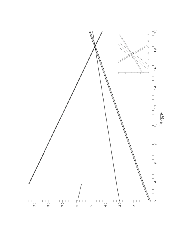
Figure 1: Running couplings in the extended left–right symmetric model with one extra pair of exotic fermion representations $(3,1,1,\frac{5}{3})_{l}\oplus(3,1,1,\frac{5}{3})_{r}$ and the Higgs sector of the doublet model, i.e. one scalar bidoublet and one pair of doublets. The left–right scale is $M_{R}=6\cdot 10^{3}$ GeV, and the GUT–scale $M_{GUT}=10^{18.4}$ GeV.

In Fig. 1 we show as an example the solution $F_{1}=1$, $H_{1}=1$, $H_{2}=1$ explicitly since it has very interesting properties. In this example we have thus one scalar bidoublet, one pair of doublets (the doublet model), and one additional fermionic pair of $(3,1,1,\frac{5}{3})_{l}\oplus(3,1,1,\frac{5}{3})_{r}$. This solution has a remarkable low left–right scale of only 6 TeV and a very high GUT–scale which is almost the Planck scale. The proton life time $\tau_{P}\approx 10^{45}$ yrs is far beyond the lower experimental bound and thus completely safe. One may ask whether such solutions with a very high $M_{GUT}$ are physical meaningful or not. Taken seriously they could point to a scenario which is usually not considered: New physics beyond $M_{R}$ at the Planck scale could make a direct transition from Planck scale physics to the left–right model without any intermediate stage. The hierarchy problem might be solved when the Planck–scale physics is expressed explicitly, but this information might also be lost completely in the low energy effective Lagrangian.

Our search was performed at the one–loop level and thresholds were described in the $\theta$–function approach with one common threshold scale. We estimate that the corrections from higher orders and threshold functions are of the order of $1\sigma$. The scale $M_{R}$ was determined always as the “best fit”, i.e., intersection of the central lines. Since $M_{R}$ is treated as a free parameter it seems always possible to absorb corrections into the precise value of $M_{R}$ as long as it is not too close to its lower or upper bound. However, the analysis of unification solutions becomes much more involved if the mass spectrum of the left–right model were widely spread around $M_{R}$. In this case special attention has to be paid for example to those solutions where $\tau_{P}$ is near the lower bound. Two–loop and threshold corrections can change the result for $\tau_{P}$ up to one order of magnitude.

In summary we have found many new possibilities of non–supersymmetric left–right models with gauge coupling unification. We required that the models are anomaly free and that the GUT–scale is below the Planck–scale, but high enough to avoid problems with proton decay. The left–right scale should lie between 1 TeV and the GUT–scale. Solutions were found even with very low left–right scale which was so far unknown. We presented a number of “minimal” solutions where the number of extra fermion and scalar representations beyond the known fermions (quarks and leptons) and gauge fields was restricted to four. There exist strong upper limits on the size of representations in order to avoid Landau singularities before the GUT–scale is reached. We demonstrated how this can be used to eliminate large representations from the search. But without limitations on the number of extra representations there are still many GUT–solutions. In an unconstrained search we found more than 1500 candidates. We think that this demonstrates that coupling unification alone is not very helpful to decide among candidates of new physics as long as one does not have a criterion for the type and number of representations.

Some of the listed models with a rather small set of “exotic particles” may be worth to be studied phenomenologically in more detail. In these studies additional investigations on the behaviour of Higgs– and Yukawa–couplings should be included. It would also be interesting to include systematically one or two more intermediate stages on the way to the GUT–scale. One could for example consider extensions of the left–right model which contain an $SU(4)\otimes SU(2)\otimes SU(2)$, originally proposed by Pati and Salam [20]. Furthermore, the impact of higher dimensional operators suppressed by the Planck scale which arise from quantum gravity or Kaluza–Klein–type theories can be taken into account. It is interesting to see that this is still compatible with a low $M_{R}$ [21].

We are grateful to E. Akhmedov and E. Schnapka for comments and useful discussions. This work was supported in part by the DFG grant Li519/2–1 and EC grant ERB SC1*CT000729.

References

-
[1]
J.C. Pati, A. Salam: Phys.Rev. D10 (1975), 275;
R.N. Mohapatra, J.C. Pati: Phys.Rev. D11 (1975), 566; 2558;
G. Senjanović, R.N. Mohapatra: Phys.Rev. D12 (1975), 1502. - [2] N. Shaban, W. Stirling: Phys.Lett. B291 (1992), 281
- [3] N. Deshpande, E. Keith, T. Rizzo: Phys.Rev.Lett. 70 (1993), 3189
- [4] E. Ma: Phys.Rev. D51 (1995), 236
- [5] E. Ma: Phys.Lett. B344 (1995), 164
-
[6]
D. Chang, R. Mohapatra, J. Gipson, R. Marshak, M. Parida:
Phys.Rev. D31 (1985), 1718 - [7] P. Frampton, S. Glashow: Phys.Lett. B131 (1983), 340 and ibid. B135 (1984), 515 (erratum)
- [8] U. Amaldi, W. de Boer, H. Fürstenau: Phys.Lett. B260 (1991), 447
-
[9]
U. Amaldi, W. de Boer, P. Frampton, H. Fürstenau, J. Liu:
Phys.Lett. B281 (1992), 374 - [10] H. Georgi, S. Glashow: Phys.Rev. D6 (1972), 429
- [11] J. Choi, R. Volkas: Phys.Rev. D45 (1992), 4261
- [12] D. Jones: Phys.Rev. D25 (1982), 581
- [13] R. Slansky: Phys.Rep. 79, No. 1 (1981), 1–128
- [14] W. McKay, J. Patera: “Tables of dimensions, indices, and branching rules for representations of simple Lie algebras”, Lecture notes in pure and applied mathematics (69), Marcel Dekker, Inc., New York and Basel (1981)
- [15] D. Bailin, A. Love: “Introduction to Gauge Field Theory”, Institute of Physics Publishing, Revised Edition 1993
- [16] W. Hollik: Invited talk at the XV Int. Conference on Physics in Collisions, Cracow, Poland, June 1995 (hep–ph/9507406)
- [17] S. Bethke: PITHA–95–14 (“Status of –Measurements”, 30th Rencontres de Moriond, Juni 1995)
- [18] Particle Data Group, Review of particle properties, in: Phys.Rev. D50 (1994), 1173–1826
- [19] E. Akhmedov, M. Lindner, E. Schnapka and J. Valle, Phys.Lett. B368 (1996), 270; Phys.Rev. D53 (1996), 2752.
- [20] J.C. Pati and A. Salam as cited in [1].
- [21] A. Datta, S. Pakvasa: Phys.Rev. D50 (1994), 2192