On the dispersive two-photon amplitude
Abstract
We present a full account of the two-loop electroweak, two-photon mediated short-distance dispersive decay amplitude. QCD corrections change the sign of this amplitude and reduce it by an order of magnitude. Thus, the QCD-corrected two-loop amplitude represents only a small fraction (with the central value of 5 %) of the one-loop weak short-distance contribution, and has the same sign. In combination with a recent measurement, the standard-model prediction of the short-distance amplitude, completed in this paper, provides a constraint on the otherwise uncertain long-distance dispersive amplitude.
Preprint BI - TP 96/08, Oslo-TP-2-96 and ZTF - 96/03
hep-ph/9605337
1 Introduction
Even before it was measured, the decay had provided valuable insight into the understanding of weak interactions. The non-observation of the decay at a rate comparable with that of showed the importance of the GIM mechanism [1]: the invention of the charmed quark made possible the necessary suppression of the amplitude. Now, equipped with the results of the new measurements and in view of the forthcoming data, we take this important amplitude under scrutiny.
The amplitudes in a free-quark calculation [2] (Fig. 1a and Fig. 1b) represented by one-loop (1L) W-box and Z-exchange diagrams, respectively, exhibited a fortuitous cancellation of the leading-order contributions. Therefore, as shown by Voloshin and Shabalin [3], one was addressed to consider the two-loop (2L) diagrams corresponding to Fig. 1c as a potentially important light-quark contribution.

The contributions shown in Fig. 1c were brought to attention by the measurements [4, 5] which indicated that the absorptive part of the diagram in Fig. 1c dominated the rate of the decay. Namely, normalizing the amplitudes to the branching ratio
| (1) |
and comparing it with the most recent BNL measurement [4]
| (2) |
exhibits the saturation by the absorptive (Im) part. It completely dominates the contribution, giving the so-called unitarity bound [6]
| (3) |
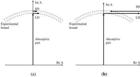
corresponding to Im. Comparing the measurement (2) with the unitarity bound (3), there is room for a total Re of order . Thus, the total real part of the amplitude, being the sum of short-distance (SD) and long-distance (LD) dispersive contributions,
| (4) |
must be relatively small compared with the absorptive part of the amplitude, as illustrated in Fig. 2. Such a small total dispersive amplitude can be realized either when the SD and LD parts are both small (Fig. 2a) or by partial cancellation between these two parts (Fig. 2b). Notably, the opposite sign of SD and LD contributions (as favoured by some calculations) leaves more space for an additional SD contribution. If the SD amplitude is found to be small, there is no room for a large LD dispersive amplitude . This leads us to reconsider previous SD calculations [3, 7] in the next section.
Frequently, the SD part has been identified as the weak contribution represented by the one-loop W-box and Z-exchange diagrams of Figs. 1a and 1b. This one-loop contribution is dominated by the -quark in the loop (proportional to the small KM-factor ), and the inclusion of QCD corrections [8, 9] does not change this amplitude essentially. In the present paper we stress that the diagram of Fig. 1c () leads to the same SD operator as that of preceding two diagrams (proportional to ). As already pointed out in [3, 10], the corresponding two-loop diagrams with two intermediate virtual photons have a short-distance part (contained in ) picking up a potentially sizable contribution from relatively high-momentum photons. The total SD amplitude is
By exploring the contribution from Fig. 1c leading to the amplitude, we isolate the strongly model-dependent LD dispersive piece. Section 2 is devoted to the calculation of the dispersive two-loop SD amplitude . In section 3 we conclude that this amplitude enables us to predict the possible range of the LD dispersive amplitude , the knowledge of which has been urged by studies of the related rare kaon decays [11].
2 Dispersive two-loop SD contribution
A complete treatment of the two-loop amplitude considered here is a missing piece in the literature. There is an enlightening feature of the diagram in Fig. 1c: the loop-momentum of the photon in Fig. 1c enables us to control the distinction between the LD and SD contributions from this diagram. We approach this problem of separating the two contributions by studying the SD piece, defined by the photon momenta above some infrared cut-off of the order of some hadronic scale . A sensible SD amplitude should have a mild dependence on the choice of the particular value of . We calculate the (two-loop) quark process
| (5) |
for which we obtain a result proportional to the left-handed quark current for the transition.

We present the main results of the calculation of the full set of 44 electroweak (EW) two-loop diagrams in the ’t Hooft-Feynman gauge. It is convenient to distinguish between three sets of diagrams, depending on one-particle irreducible subloops – the -diagrams given by transitions (of the type shown in Fig. 3), the -diagrams given by the transition (illustrated in Fig. 4) and the -diagrams given by the non-diagonal transition (shown in Fig. 5).


We stress that the electroweak insertions are finite, whereas the divergent and insertions require a proper regularization. For the external light quarks at hand, we have used the on-shell subtraction in the limit of vanishing external 4-momenta. The structure for -diagrams corresponds to the amplitude regularized to be zero at the mass shells of the - and -quarks [12], in the limit , in which we work.
After regularization, the effective (-transition), (-transition) and (-transition) have the structures
| (6) |
where is the photon-loop momentum (which for - and -diagrams coincides with the - or -quark momentum inside the loop). After regularization, all three types of diagrams are internally gauge invariant with respect to QED when diagrams with crossed photons are added. Other structures, besides those in (6), are present for () and () diagrams, but do not contribute to the two-loop quark process (5) when diagrams with crossed and uncrossed photons are summed.
The two-loop amplitude resulting from the , and subloops in (6) acquires the form
| (7) |
which is proportional to the same operator as that appearing in the one-loop amplitude [8, 9]. Summing over the quark flavours () in the loop gives us a general amplitude as
| (8) | |||||
explicitly exposing the GIM mechanism (the ’s are the appropriate KM factors). After embedding the () in the meson (), the physical CP-conserving amplitude takes the form
| (9) |
For the light quarks (), diagrams (Fig. 3a) and (Fig. 4) dominate completely (and are therefore under scrutiny in Table 1), the other diagrams being suppressed by an extra factor after the GIM mechanism has been taken into account. For the heavy quark () in the loop, such a suppression is of course absent, and we a priori have to consider all diagrams. It turns out that then the largest contribution among -diagrams is (Fig. 3b), and among -diagrams the largest is again . Both in the light- and heavy-quark cases there are also the contributions from the non-diagonal self-energy (-diagrams). Being negligible in the pure electroweak case (suppressed by for light quarks after GIM), the off-diagonal self-energy contribution becomes potentially unsuppressed () when perturbative QCD is switched on [13] (Fig. 5).
2.1 Pure electroweak results
Let us first display the pure electroweak (EW) results in order to keep contact with the early calculation by Voloshin and Shabalin [3]. We have calculated all the contributions numerically, the results of the dominating ones being presented in Table 1. In addition, the analytical expressions can be obtained in the light-quark () case. Let us display the analytic forms for the leading and amplitudes which reproduce those obtained previously [3]. Our calculation shows that, for , the leading logarithmic (LL) contribution in the pure electroweak case is
| (10) |
where is the infrared cut-off, defined above. In this way we avoid integrals over low photon momenta, which correspond to some LD contributions. For the amplitude , we obtain the following LL result for the single quark loop (for ):
| (11) | |||||
Taken at face value, the expressions (10) and (11) are the result for the -quark case (). The corresponding -quark contribution is obtained by the replacement . These results conform to [3] after the GIM mechanism has been taken into account.
As a new contribution to the existing literature, we have also performed the 2L calculation of the electroweak diagrams for the heavy quarks () in the loop. In this case, the dominant contributions are (Fig. 3b) and (Fig. 4). However, these are associated with the small KM factor and are therefore suppressed. Table 1 displays only these dominant amplitudes and the total amplitudes, a full account being relegated to a more detailed publication [14]. This table also illustrates a mild sensitivity of the dominant light-quark electroweak amplitudes and to the IR cut-off . As we have also displayed the total amplitude, this table illustrates to what degree the indicated contributions are dominant within the full set of the pure EW diagrams. The agreement between the numerical ( and ) and the analytical LL results (10) and (11), after performing the GIM procedure, is explicated by the corresponding rows of Table 2. The last row of Table 1, normalized to the measured amplitude, shows the largeness of the net EW contribution. We observe that such a large pure electroweak 2L contribution would have decreased the one loop amplitude [9] substantially.
| Dominant | Pure EW | Dominant | Pure EW | ||
|---|---|---|---|---|---|
| diagram | diagram | ||||
| 1.86 | 1.22 | 23.8 | 22.7 | ||
| total | 1.90 | 1.25 | total | 27.1 | 26.4 |
| 1.70 | 1.04 | 20.6 | 19.1 | ||
| total | 1.70 | 1.03 | total | 15.6 | 14.2 |
| Total | 3.59 | 2.28 | Total | 42.7 | 40.7 |
| Re | 1.55 | 0.98 | Re | 0.017 | 0.016 |
2.2 QCD corrections
There are some subtleties in performing QCD corrections to the two-loop diagrams considered. Although the gluon corrections pertain to the quark loop, the highly off-shell photons closing the other (quark-lepton) loop control the SD regime of the two-loop amplitude as a whole. In general, there is up to one log per loop, as exemplified by the -term in (11) related to Fig. 4.
There is a suitable prescription introduced in Refs. [8, 15] and applied by other groups [16, 17, 18] for handling the leading QCD corrections. Using this prescription, one can write the amplitude as an integral over virtual quark loop momenta. In the problem considered, we have to decode the 2-loop momentum flow in order to extract the leading logarithmic structure, which we then sum using the renormalization-group technique. Thereby, we refer to the building blocks considered previously – the electromagnetic penguin of Ref. [19] (now appearing in the amplitude), the QCD corrections to the quark-loop of Fig. 3a [20] and to a very recent treatment of the self-penguin [21]. Let us present this in more detail.
We start by demonstrating the QCD corrections to the - and -quark loops of -diagrams in Table 2. One first hunts the leading log which should correspond to the -term in (10). This result can be understood from the result of the previous calculation [20], which consisted of two terms dominated at the scales and , respectively. Moreover, these two terms had the relative weights 1 and , respectively. When this amplitude is inserted in to the two-loop diagram for , we gain one logarithm. Since the two terms in (10) stem from the loop integrals dominated by the momenta at and , respectively, the QCD-corrected amplitude acquires the form
| (12) |
which in principle agrees with [3] and disagrees with [7]. Here, the QCD coefficient reflects the colour-singlet nature of the photonic part of the diagram, and is given by
| (13) |
where are the Wilson coefficients of the 4-quark operators in the effective Lagrangian of Ref. [22]. In the leading logarithmic approximation they are given by
| (14) |
where and are the anomalous dimensions and , being the number of active flavours. In contradistinction to the numerically favourable and stable colour-octet factor , the singlet coefficient (13) is rather sensitive to the choice of , with a notable switch of the sign [15, 17] for at the scale of a few GeV2. Combining the - and -quark contributions by taking into account the GIM mechanism (see (8)), only the second term in (12) survives.
The amplitude in (11) can be understood in terms of the electromagnetic penguin subloop, which is, within the LL expansion, proportional to
| (15) |
where is the momentum of virtual photons. Inserting this subloop into the next loop, we gain one logarithm (in particular, ln ln). Hence the form in the second term in (11), which leads to the QCD-corrected amplitude expressed in an integral form as
| (16) | |||||
Again, the expressions (12) and (16) apply directly to the -quark contribution, the -quark contribution being obtained by making the replacement . This means that when taking into account the GIM mechanism, the integral in (16) will run from to . The net result of the QCD dressing is similar to that for the diagram: a suppressed amplitude with a change of sign.
The -contribution stemming from the QCD-induced self-penguin () in Fig. 5. might also be interesting. As opposed to and contributions it is not suppressed by the colour singlet factor , but contains the numerically favourable colour octet factor . It is, however, suppressed by . For the case, we obtain to all orders in QCD
| (17) | |||||
where . In addition, 7/162 is an overall loop factor, and the terms 5/6 have the same origin as in (15) and (16). The -quark contribution is again obtained by making the replacement .
The light-quark approximation () is used in (17). For an arbitrary quark mass, needed to treat the heavy top in the loop, the calculations are much more difficult [21]. We have done an estimate and found that the top-quark contribution is roughly 10 of the charm-quark contribution (taking into account that at is about 1/3 of at .).
Table 2 displays a detailed structure of the dominant amplitudes from Table 1, before and after applying the GIM mechanism: the first, the second, and the third block of the table display the , , and contributions, respectively. In the third block, and refer to the bare and dressed self-penguin contributions, respectively, whereas refers to the negligible pure electroweak (EW) contribution. Therefore, is different from . As a curiosity, we have found that the latter has a peculiar GIM cancellation: there is an exact cancellation between the -quark contribution for and the -quark contribution for . As a result, is not so GIM-relaxed as expected for a heavy-quark case .
| EW + SD QCD | EW + SD QCD | ||||||
|---|---|---|---|---|---|---|---|
| -loop | -loop | GIM | -loop | -loop | GIM | ||
| -2.14 | -3.57 | 1.42 | -17.4 | -40.4 | 23.0 | ||
| -4.52 | -6.09 | 1.58 | -22.3 | -18.3 | -4.0 | ||
| -6.19 | -6.09 | -0.10 | -22.3 | -18.3 | -4.0 | ||
| -20.4 | -21.6 | 1.24 | -0.8 | -20.4 | 19.6 | ||
| -20.8 | -22.0 | 1.19 | -2.0 | -20.8 | 18.8 | ||
| -14.9 | -14.7 | -0.23 | -2.0 | -14.9 | 12.9 | ||
| -0.61 | -0.61 | -0.52 | -0.61 | 0.09 | |||
| 0.46 | 0.47 | -0.01 | 0.47 | ||||
| 0.47 | 0.48 | -0.01 | 0.47 | ||||
3 Conclusions
In this paper we have focused on the 2-loop (2L) contributions, leading to the typical SD local operator for the quark transition but also having a LD (soft-photon) range. Our approach starts from the SD side, whereby an infrared (IR) cut-off of virtual photons sets in. We contrast the SD contribution with the complementary LD ones, which have to be calculated using other methods, and are rather model dependent at the present stage. The numerically important 2L pure electroweak SD contributions are due to the light () quarks in the loop. Besides completing the previous calculation for light quarks, we have also considered the 2L diagrams including the heavy () quarks. A large number of electroweak diagrams may compensate for a small CKM factor, and one might expect non-negligible effects. However, the actual calculation shows that the various amplitudes have different signs, and taking into account the smallness of , the heavy-quark contribution is negligible.
Next, we have shown the importance of the SD QCD corrections for the 2L diagrams, summarized in Fig. 6.
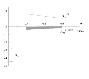
i) smoothens the -dependence (making the SD extraction better defined),
ii) changes the sign (making it coherent to the 1L amplitude), and
iii) suppresses it to large extent
Inclusion of these QCD corrections appears to be subtle and more dramatic than it was the case for the 1L diagrams. Two decades ago there was a controversy concerning QCD corrections to these 1L diagrams. Ref. [8] resolved it by an adequate treatment of the loop integrals. Our results for SD corrections to the 2L diagrams are shown in Table 2. The short-distance QCD corrections suppress the part of the SD amplitude which is electroweakly dominant before inclusion of QCD corrections. The basic reason for this is the behaviour of the QCD coefficient. In particular, the and amplitudes are suppressed to a large extent, and do not anymore interfere destructively with the 1L SD amplitude of Ref. [9]. Without this suppression, the scenario of Fig. 2a would appear as a more likely one.
We should stress that in the treatment of the 2L amplitude we have performed QCD corrections in the leading logarithmic approximation by using (14), while the 1L amplitude was treated in the next to leading (NLO) approximation in [9].
To summarize, we have found a modest light-quark 2L contribution stemming from intermediate virtual photons having relatively high momentum. Introducing the error bars corresponding to in the range 0.7–0.9 GeV, and a more essential one from empirical uncertainty in (corresponding to in the range 150–250 MeV), we obtain
| (18) |
This has the same sign and, for central values, corresponds to 5 % of [9],
| (19) |
where the uncertainty mainly reflects the poor knowledge of . Although the 1L and 2L contributions are not treated on an equal footing (NLO versus LL QCD corrections), this result still enables us to estimate the size of from (4). Referring to our comments below (3), and allowing for a , we find the following allowed range for :
| (20) |
Thus, having a dispersive LD part of the size comparable with the absorptive part [24] is still not ruled out completely.
The two vector-meson dominance calculations for the LD amplitude considered as the referent calculations in Ref. [4] have basically opposite signs:
On the basis of the inferred relative sign between 1L and 2L contributions, Ref. [7], attempted to discriminate between the two LD calculations quoted above. (They favoured Ref. [25], and disfavoured Ref. [26] as the one ascribing opposite signs to SD and LD.) In the last of their papers [7] they even concluded that the BNL measurements [4] were in conflict with the standard model.
We have found that these conclusions are doubtful, since they are based on an erroneous SD extension to the LD momentum region. In our opinion, Ref. [7] misidentifies what (according to the calculational method employed) should be their SD amplitude , with . In our treatment (see section 2) we have avoided the forbidden low-momentum region by introducing the infrared cut-off of the order of the -mass. We have demonstrated that there is a subtle QCD suppression of the originally quite sizable SD EW 2L amplitude. Therefore, a real amplitude of a considerable size given in (20) corresponding to low -momenta ( and below), is still allowed. This might be used as a consistency check for the methods of the type employed in Refs. [25, 26].
Taking into account the difficulties inherent to the estimates of the LD amplitude, it is welcome to arrive at the constraint (20). Accordingly, provided the sign of are correctly given in [4], the BNL experiment combined with the standard-model calculation tends to favour the result of Ref. [26]. In this way, the scenario of Fig. 2b seems to be preferred by the standard model. Provided that the beyond-standard-model effects are represented by the relatively small SD amplitudes, this scenario hinders the possibility of recovering such effects in the decay. The forthcoming data from measurements [27] will further test the conclusions of the present paper.
Acknowledgement
Two of us (K.K. and I.P.) gratefully acknowledge the partial support of the EU contract CI1*-CT91-0893 (HSMU) and the hospitality of the Physics Department of the Bielefeld University. One of us (I.P.) would also like to acknowledge the hospitality of the Department of Physics in Oslo, and to thank the Norwegian Research Council for a traveling grant.
References
- [1] S.L. Glashow, J. Iliopoulos and L. Maiani, Phys. Rev. D2 (1970) 1285.
- [2] M.K. Gaillard and B.W. Lee, Phys. Rev. D10 (1974) 897; M.K. Gaillard, B.W. Lee and R.E. Shrock, Phys. Rev. D13 (1976) 2674.
- [3] M.B. Voloshin and E.P. Shabalin, JETP Lett. 23 (1976) 107 [Pis’ma Zh. Eksp. Teor. Fiz. 23 (1976) 123].
- [4] A.P. Heinson et al. (BNL E791), Phys. Rev. D51 (1995) 985.
- [5] T. Akagi et al., Phys. Rev. Lett. 67 (1991) 2618.
- [6] L.M. Sehgal, Phys. Rev. 183 (1969) 1511; B.R. Martin, E. de Rafael and J. Smith, Phys. Rev. D2 (1970) 179.
- [7] A.M. Gvozdev, N.V. Mikheev and L.A. Vassilevskaya, Phys. Lett. B274 (1992) 205; Sov. J. Nucl. Phys. 53 (1991) 1030 [Yad. Fiz. 53 (1991) 1682]; hep-ph/9511366.
- [8] A.I. Vainstein, V.I. Zakharov, V.A. Novikov and M.A. Shifman, Yad. Fiz. 23 (1976) 1024 [Sov. J. Nucl. Phys. 23 (1976) 540]; V.A. Novikov, M.A. Shifman, A.I. Vainstein and V.I. Zakharov, Phys. Rev. D16 (1977) 223.
- [9] G. Buchalla, A.J. Buras, Nucl. Phys. B412 (1994) 106; G. Buchalla, A.J. Buras and M.E. Lautenbacher, Rev. Mod. Phys. 68 (1996) 1125; G. Buchalla, hep-ph/9701377.
- [10] R.E. Shrock and M.B. Voloshin, Phys. Lett. B87 (1979) 375.
- [11] J.F. Donoghue and F. Gabbiani, Phys. Rev. D51 (1995) 2187; G. D’Ambrosio and J. Portolés, Nucl. Phys. B492 (1997) 417.
- [12] E.P. Shabalin, Yad. Fiz. 32 (1980) 249 [Sov. J. Nucl. Phys. 32 (1980) 129].
- [13] E.P. Shabalin, ITEP 86-112; B. Guberina, R.D. Peccei and I. Picek, Phys. Lett. B188 (1987) 258; J.O. Eeg, Phys. Lett. B196 (1987) 87.
- [14] J.O. Eeg, K. Kumerički and I. Picek, in preparation.
- [15] A.I. Vainstein, V.I. Zakharov, L.B. Okun’, and M. A. Shifman, Yad. Fiz. 24 (1976) 820 [Sov. J. Nucl. Phys. 24 (1976) 427].
- [16] W.A. Bardeen, A.J. Buras and J.-M. Gerard, Nucl. Phys. B293 (1987) 787; A. Pich and E. de Rafael, Nucl. Phys. B358 (1991) 311.
- [17] J.O. Eeg, Phys. Rev. D23 (1981) 2596.
- [18] I. Picek, Nucl. Phys B (Proc. Suppl.) A24 (1991) 101.
- [19] J.O. Eeg and I. Picek, Phys. Lett. B214 (1988) 651.
- [20] J.O. Eeg, B. Nižić and I. Picek, Phys. Lett. B244 (1990) 513.
- [21] A.E. Bergan and J.O. Eeg, Phys. Lett. B390 (1997) 420.
- [22] M.K. Gaillard and B.W. Lee, Phys. Rev. Lett. 33 (1974) 108; G. Altarelli and L. Maiani, Phys. Lett. B52 (1974) 35.
- [23] Particle Data Group, Phys. Rev. D54 (1996) 1.
- [24] G. D’Ambrosio and D. Espriu, Phys. Lett. B175 (1986) 237.
- [25] L. Bergström, E. Massó and P. Singer, Phys. Lett. B249 (1990) 141.
- [26] P. Ko, Phys. Rev. D45 (1992) 174.
- [27] P. Franzini, hep-ex/9512005, Proc. of the 17th International Symposium on Lepton-Photon Interactions, Beijing 1995, World Scientific, Singapore 1996, p. 414.