PM/96-14
May 1996

We consider the virtual effects of a general type of Anomalous (triple) Gauge Couplings on various experimental observables in the process of electron-positron annihilation into a final fermion-antifermion state. We show that the use of a recently proposed ”$Z$-peak subtracted” theoretical description of the process allows to reduce substantially the number of relevant parameters of the model, so that a calculation of observability limits can be performed in a rather simple way. As an illustration of our approach, we discuss the cases of future measurements at LEP2 and at a new 500 GeV linear collider.

1 Introduction

Among the various sources of deviations from the Standard Model (SM), the one that considers the possibility of anomalous triple gauge boson couplings (AGC) has been very extensively examined and discussed in recent years. Starting from the undeniable consideration that for the $WWZ$ and the $WW\gamma$ couplings no stringent experimental test of the SM predictions is yet available, several models have been proposed [1] that would predict, or accomodate, possible differences from the SM canonical values, leading to observable effects both in present and in future measurements.

On this very last topics, some theoretical debate has occurred, concentrated on the very relevant question of whether the already available information from experiments at low energy and on $Z$-resonance peak could, or could not, be improved by a certain set of future experiments, in particular by those performable at LEP2, for this special type of models [2],[3],[4]. As a result of long and interesting discussions, it has been generally recognized that if the deviations from the SM are fully incorporated into a theoretical mechanism that retains the original $SU(2)\times U(1)$ gauge invariance even at a large scale $\Lambda$ where the SM looses its validity, the available bounds on the parameters of such models are ”mild”. One might expect, therefore, that future experiments at more powerful machines with a suitable experimental accuracy would improve the bounds for all the parameters, and that the overall improvement would be automatically guaranteed by moving to higher and higher energy accelerators. In this picture, one would guess that a separate analysis of the final two boson and two fermion channels would lead to increased bounds for the complete set of parameters, since some of them would only contribute the first channel, while the remaining ones would be mainly determined by the second one. In practice, the final bosonic channel will be investigated both at $e^{+}e^{-}$ and at $pp$, $p\bar{p}$ colliders. For the second one, whose analysis requires one loop electroweak effects, the requested precision should select the $e^{+}e^{-}$ colliders as the only source of possible information. The combined investigations at the two types of colliders should then lead to a better and better determination of all the parameters of the model.

The aim of our paper is to show that this is not always necessarily the case. To be more specific, we will show that the previous expectation will be certainly justified for a special subset of model parameters, for which the bounds should indeed monotonically increase with c.m. energy . On the contrary, other parameters do not seem to enjoy this property. These are those parameters that contribute the final two fermion channel and that can be reabsorbed in the definition of LEP1-SLC measured quantities. In this case, the relative accuracy of the future $e^{+}e^{-}$ colliders is beaten (in a certain sense that will be illustrated) by Z-peak measurements. In a sense, there appears to be a natural and easy criterion to distinguish those parameters whose knowledge can be improved by future accelerators from those for which this would not be the case.

In practice, to make this general discussion more explicit, we shall need a concrete example. With this aim, we shall resort in this paper to a specific representative model, that describes the low energy effects of a certain unknown new physics, appearing at scale $\Lambda$, by an effective Lagrangian built by dimension six operators only [2],[5]. We shall stick from now on to the notations of ref.[5], and devote the interested reader to that paper for a much more exhaustive discussion of the main points that we have tried to summarize here.

A first, and apparently purely technical, problem immediately arises if one fully accepts the philosophy and the framework of ref.[5]. This is related to the relatively large number of parameters that the model introduces. To describe a four-fermion process like that of electron-positron annihilation into fermion-antifermion at arbitrary energy, four renormalized parameters are requested at the one loop level. To these quantities, that are specific of the model, one must also add at the considered level the unknown Higgs mass and the still not extremely precisely determined top mass, that introduce a small but not really negligible extra theoretical error in all the fits that try to fix the values of the four anomalous couplings. Since the number of adequately precise experimental measurements at such future (including LEP2) electron-positron colliders is unavoidably limited, a conventional program of derivation of bounds requires some care (as it was shown in an excellent way in a recent publication[6]). At the same time, it appears rather cumbersome to individuate possible features of experimental effects that would be characteristic of this model (like a definit sign in some deviation, or special correlations of effects in different observables) and that would allow, in case of a visible signal, to differentiate the model in a clean way from other sources of virtual signals.

In this short paper we first show that these difficulties can be greatly reduced if the ”conventional” theoretical description of the considered process is abandoned and a different one, recently proposed and denominated ”$Z$-peak subtracted” representation, is utilized. To be more precise, we shall briefly review in the next Section 2 the main features of this representation, showing that, as an immediate consequence of adopting it, only two parameters of the considered model (without extra top or Higgs mass dependence) remain in the theoretical expressions. As a benefit of this simplification, a much simpler two-parameter fit to the data will be now performable. In Section 3 we shall give the results of our analysis for the specific cases of LEP2 and of a future 500 Gev linear collider (NLC). We shall calculate in a realistic way, that takes into account the potentially dangerous effects of QED radiation, the effects of the model on various observables and the limits in the plane of the two surviving parameters.

From our reduction of the number of involved parameters, a second benefit can be derived since it will now be possible to draw in a $3-d$ space of effects on three different and suitable observables a region that will be completely characteristic of this model. If other competitor models admit a theoretical representation of their effect on the same observables where also only two parameters are involved, they will also be associated in the previous space to a certain region. In Section 4 we shall show that, at least for the two very general models of ”technicolour” type and of ”extra $Z$” type, the corresponding regions (that we shall call ”reservations”) would not overlap. This would allow to identify the AGC model, if a virtual signal were seen, in a relatively clean way, at least with respect to the two previously mentioned general competitor models.

Having shown with a specific example that a sensible reduction of the number of AGC parameters is indeed possible, we shall devote the final Section 5 to a short discussion of the possible generalization of our approach to more complicated cases. We shall try to give reasonable arguments in favour of the possibility of a systematic classification that would represent a clean compromise between low energy and higher energy constraints for this type of theoretical models.

2 The method

The theoretical description of the process $e^{+}e^{-}\to f\bar{f}$ (here $f$ is a general fermion) that we follow in this paper has been fully illustrated in two previous publications, treating separately the case of final lepton [7] and quark [9] production. In this Section we shall only illustrate with one representative example the main features and consequences of our approach.

In the theoretical description of the process commonly used at the one loop level, the invariant scattering amplitude is written as the sum of a ”Born” term and additional higher order ”corrections”. The input parameters of the Born term are by convention $\alpha$ (the electric charge, measured at zero momentum transfer), $M_{Z}$ (the $Z$ mass) and $G_{\mu}$, the Fermi constant defined by the muon lifetime and known to a relative accuracy of about 2.$10^{-5}$, practically the same as that now available for the measurement of the $Z$ mass. The very high accuracy of the experimental determination of these parameters, that enter as theoretical input the SM predictions, guarantees that the latter are not affected by unwanted ambiguities. This is particularly relevant for the set of high precision measurements performed with the aim of testing the SM by looking for extra virtual effects on top of $Z$ resonance, where the available experimental precision for several observables has now reached values of a relative few permille. Clearly, in this situation, the replacement in the starting theoretical expressions of $G_{\mu}$ by a different input parameter known, for instance, at the level of a relative few permille would not be a productive move.

A priori, this rather quantitative consideration does not necessarily apply for the situation of possible searches of virtual effects beyond the SM at future $e^{+}e^{-}$ colliders, i.e. at LEP2 and at a 500 GeV NLC. Here the results of a series of dedicated analyses [10], [11] show that the realistic experimental precision to be expected for several relevant observables will be of the order of a relative few percent. From a purely pragmatic point of view, replacing $G_{\mu}$ by a parameter known at the few permille level would not lead, in this case, to negative consequences. It is not difficult to show that the aforementioned replacement might also lead to interesting positive consequences, for suitable choices of the new parameter(s). To make this statement more precise, we shall consider in this paper the illustrative and particularly simple example of the pure $Z$ contribution to the cross section of the process of $e^{+}e^{-}$ annihilation into a couple of muons, at squared total c.m. energy $=q^{2}$. At the relevant one loop level the latter can be written as :

$$\sigma_{\mu}^{(1)(zz)}(q^{2}) = (\frac{4}{3}\pi\,q^{2})\left|\frac{\sqrt{2}}{4\pi}\,g^{2}_{A\ell,0}\,\right.\left(1+(1-4\tilde{s}^{2}_{\ell}(q^{2}))^{2}\right)\times$$ (1)

$$\times \frac{G_{\mu}M^{2}_{z}}{[q^{2}-M^{2}_{z}+i\,M_{z}\Gamma_{z}(q^{2})]}\,\left(1+\frac{\delta G_{\mu}}{G_{\mu}}+\right.\left.\left.+{\cal R}e\,\frac{\tilde{A}_{z}(0)}{M^{2}_{z}}-\tilde{I}_{z}(q^{2})\right)\right|^{2}$$

where $g^{2}_{Al,0}={1\over 4}$ and the remaining quantities are defined as follows. Denoting as $\tilde{A}_{i}(q^{2},\theta)$ ($i=\gamma,Z,\gamma Z$) a certain gauge-invariant combination of transverse self-energy, vertices and boxes, that we always built following the Degrassi-Sirlin prescription [12], and following the definition

$$A_{i}(q^{2},\theta)\equiv A_{i}(0,\theta)+q^{2}F_{i}(q^{2},\theta)$$ (2)

$s^{2}_{l}(q^{2})$ is the result of the integration over $cos\theta$ in the differential cross section of the quantity

$$\tilde{s}^{2}(q^{2},\theta)\equiv s^{2}_{1}(1+\tilde{\Delta}\kappa^{1}(q^{2},\theta))$$ (3)

with

$$\tilde{\Delta}\kappa^{1}(q^{2},\theta)={c_{1}\over s_{1}}\tilde{F}^{(lf)}_{\gamma Z}(q^{2},\theta)+{c^{2}_{1}\over c^{2}_{1}-s^{2}_{1}}({\Delta\alpha\over\alpha}-{\Delta G_{\mu}\over G_{\mu}}-{\Delta M^{2}_{Z}\over M^{2}_{Z}})$$ (4)

where $\Delta\alpha,\Delta G_{\mu},\Delta M^{2}_{Z}$ are the shifts from the bare quantities $\alpha_{0},\;G_{\mu 0},M^{2}_{0Z}$ to the corresponding physical ones and $s^{2}_{1}\equiv 1-c^{2}_{1}$, $s^{2}_{1}c^{2}_{1}=\frac{\pi\alpha}{\sqrt{2}G_{\mu}M^{2}_{Z}}$.

$\tilde{I}_{Z}(q^{2})$ is the result of the analogous operation on the quantity

$$\tilde{I}_{Z}(q^{2},\theta)={q^{2}\over q^{2}-M^{2}_{Z}}[\tilde{F}_{Z}(q^{2},\theta)-\tilde{F}_{Z}(M^{2}_{Z},\theta)]$$ (5)

The possibility of replacing $G_{\mu}$ by a different parameter in eq.(1) is provided by the observation that the rigourous equality holds, that defines the leptonic $Z$-width $\Gamma_{l}$ :

$$\Gamma_{l}=({\sqrt{2}G_{\mu}M^{3}_{Z}\over 48\pi})[1+\epsilon_{1}][1+(1-4s^{2}_{l}(M^{2}_{Z}))^{2}](1+\delta_{QED})$$ (6)

where $\epsilon_{1}$ is the Altarelli-Barbieri parameter [13] :

$$\epsilon_{1}\equiv{\delta G_{\mu}\over G_{\mu}}+Re\{{\tilde{A}_{Z}(0)\over M^{2}_{Z}}\}-\tilde{I}_{Z}(M^{2}_{Z})$$ (7)

and $s^{2}_{eff}(M^{2}_{Z})\equiv\tilde{s}^{2}_{l}(M^{2}_{Z})$ is the effective weak mixing angle measured al LEP1/SLC by means of the leptonic couplings.

Thus, by properly ”subtracting” in eq.(1) the combinations $\tilde{I}_{Z}(m^{2}_{Z})$ and $\tilde{s}^{2}_{l}(M^{2}_{Z})$ calculated at the $Z$ peak one can rewrite eq.(1) in the perfectly identical way :

$$\sigma_{\mu}^{(1)(zz)}(q^{2}) = \left(\frac{4}{3}\pi\,q^{2}\right)\,\left[\frac{3\Gamma_{\ell}}{M_{z}}\right]^{2}\times$$ (8)

$$\times \frac{1}{[(q^{2}-M^{2}_{z})^{2}+M^{2}_{z}\Gamma_{z}^{2}]}\,\left[1-2R(q^{2})-\frac{16(1-4s^{2}_{1})c_{1}s_{1}V(q^{2})}{[1+(1-4\tilde{s}^{2}_{\ell}(M^{2}_{z}))^{2}]}\right]$$

where :

$$R(q^{2})\equiv\tilde{I}_{Z}(q^{2})-\tilde{I}_{Z}(M^{2}_{Z})$$ (9)

$$V(q^{2})\equiv Re[F_{\gamma Z}(q^{2})-F_{\gamma Z}(M^{2}_{Z})$$ (10)

We can summarize the results of this operation as follows. At one loop, $G_{\mu}$ can be ”traded” for $\Gamma_{l}$ and $s^{2}_{eff}(M^{2}_{Z})$ in the expression of $\sigma_{\mu}$. As a consequence of this exchange, the ”corrections” $\tilde{I}_{Z}(q^{2})$, $F_{\gamma Z}(q^{2})$, are replaced by two ”$Z$-peak subtracted” functions $R,V$ and no other $q^{2}$-independent one-loop theoretical parameters (${\delta G_{\mu}\over G_{\mu}}$, ${\tilde{A}_{Z}(0)\over M^{2}_{Z}}$, ${\Delta\alpha\over\alpha}$, …etc) survive, since they have all been reabsorbed in the definition of the two measured quantities $\Gamma_{l}$, $s^{2}_{eff}(M^{2}_{Z})$.

The previous discussion applies to the ”pure $Z$” contribution to the muon cross section. For what concerns the two other contributions of ”pure $\gamma$” and of ”$\gamma-Z$” type one easily sees that only one more ”canonical” generalized function $\tilde{\Delta}_{\alpha}(q^{2})$ , already subtracted at the ”$\gamma$ peak” and entering the photon term, is required at one loop. This function is conventionally defined as the result of the $cos\theta$-integration on the generalized quantity $\tilde{F}_{\gamma}(0,\theta)-\tilde{F}_{\gamma}(q^{2},\theta)$ , as one can easily understand from the previous discussion, and we shall treat it in the usual way without extra theoretical tricks. The three functions $R(q^{2})$, $V(q^{2})$ and $\tilde{\Delta}_{\alpha}(q^{2})$ together with $\Gamma_{l}$ and $s^{2}_{eff}(M^{2}_{Z})$ are thus providing at one loop a full theoretical description for the electroweak component of the muon cross section. This conclusion is valid also for the most general observables (polarized and unpolarized asymmetries) that can be measured in the final charged lepton channel at future $e^{+}e^{-}$ colliders.

We are now already in a position to show the practical effects of the used representation for what concerns the calculations of the effects of the model of AGC ref.[5] that are considered in this paper. Although a complete discussion has been already given in Ref.[7], Section 3, we show here with the purpose of being reasonably self-contained the example that corresponds again to the $Z$-components of $\sigma_{\mu}$, eq.(1), and we choose the particularly illustrative case of the term contained in the second round bracket. By a lengthy but straightforward calculation of the relevant combinations of self-energies and vertices that make up the gauge-invariant combination, one is led to the result :

$$\left[\left(\frac{\delta G_{\mu}}{G_{\mu}}+{\cal R}e\,\frac{\tilde{A}_{z}(0)}{M^{2}_{z}}\right)-\tilde{I}_{z}(q^{2})\right]^{(AGC)}=\left[\left(\frac{-2M^{2}_{W}}{g^{2}\Lambda^{2}}\,f^{r}_{\phi,1}\right)-8\pi\alpha\,\frac{q^{2}}{\Lambda^{2}}\,\left(\frac{c^{2}_{1}}{s^{2}_{1}}\,f^{r}_{DW}+\frac{s^{2}_{1}}{c^{2}_{1}}\,f^{r}_{DB}\right)\right]$$ (11)

A glance to eq.(11) shows that it contains three of the four renormalized parameters of the model, defined in ref.[5] as $f^{r}_{\phi,1},f^{r}_{DW},f^{r}_{DB}$. In the $Z$-peak subtracted representation, eq.(8), the term eq.(11) is replaced by the subtracted functions $R(q^{2})$, whose expression in the model is :

$$R^{(AGC)}(q^{2})=8\pi\alpha\,\frac{(q^{2}-M^{2}_{z})}{\Lambda^{2}}\,\left[\frac{c^{2}_{1}}{s^{2}_{1}}\,f^{r}_{DW}+\frac{s^{2}_{1}}{c^{2}_{1}}\,f^{r}_{DB}\right]$$ (12)

As one sees, $R(q^{2})$ retains only two of the parameters, i.e. $f^{r}_{DW},f^{r}_{DB}$. The simple reason for this is that the third parameter $f^{r}_{\phi,1}$ has been reabsorbed in the measured expression of $\Gamma_{l}$. Only the two parameters that contribute the non constant part of $\tilde{F}_{Z}(q^{2})$ survive in the subtraction procedure.

It is rather easy to show that the same feature characterizes the expressions of the two extra subtracted functions $V(q^{2})$ and $\tilde{\Delta}_{\alpha}(q^{2})$

$$\tilde{\Delta}^{(AGC)}_{\alpha}(q^{2})=-8\pi\alpha\,\frac{q^{2}}{\Lambda^{2}}\,\left[f^{r}_{DW}+f^{r}_{DB}\right]$$ (13)

$$V^{(AGC)}(q^{2})=8\pi\alpha\,\frac{(q^{2}-M^{2}_{z})}{\Lambda^{2}}\,\left[\frac{c_{1}}{s_{1}}\,f^{r}_{DW}-\frac{s_{1}}{c_{1}}\,f^{r}_{DB}\right]$$ (14)

and that the same two parameters will appear, in different linear combinations, in all the three cases i.e. in all the observables of the final charged lepton channel. This already remarkable fact can be actually generalized to any observable of a final hadronic channel generated by the five light ($u,d,s,c,b$) quarks [9]. The reason that makes this useful simplification possible is the fact that in this specific model the contribution to vertices are of universal type for massless quarks. The only difference with respect to the leptonic case will be that now the new ”effective” Born approximation will contain hadronic $Z$ width and asymmetries, measured on top of $Z$ resonance.

The final point that has been investigated inRefs.[7] and [9] is that of whether the replacement of $G_{\mu}$ with the set of $Z$ peak observables does not introduce dangerous theoretical errors. The answer is that, at the expected experimental accuracy of LEP2 and NLC [10], [11] this replacement is harmless. In conclusion we are in a position to perform a detailed analysis of the effect of the considered model on the possible realistic observables. With this aim, for sake of completeness we list below approximate expressions of the various quantities in the model (the complete and rigorous expressions can be found in ref.[7],[9]) valid at LEP2, NLC energies.

The muonic cross section:

$$\sigma_{\mu}(q^{2}) = \sigma^{Born}_{\mu}(q^{2})\bigm{\{}1+{2\over\kappa^{2}(q^{2}-M^{2}_{Z})^{2}+q^{4}}[\kappa^{2}(q^{2}-M^{2}_{Z})^{2}\tilde{\Delta}\alpha(q^{2})$$ (15)

$$-q^{4}(R(q^{2})+{1\over 2}V(q^{2}))]\bigm{\}}$$

where $\kappa\equiv{\alpha M_{Z}\over 3\Gamma_{l}}\simeq 2.64$ and

$$\sigma^{Born}_{\mu}(q^{2})={4\pi\alpha^{2}\over 3q^{2}}[{q^{4}+\kappa^{2}(q^{2}-M^{2}_{Z})^{2}\over\kappa^{2}(q^{2}-M^{2}_{Z})^{2}}]$$ (16)

The muonic forward-backward asymmetry:

$$A_{FB,\mu}(q^{2}) = A^{Born}_{FB,\mu}(q^{2})\bigm{\{}1+{q^{4}-\kappa^{2}(q^{2}-M^{2}_{Z})^{2}\over\kappa^{2}(q^{2}-M^{2}_{Z})^{2}+q^{4}}[\tilde{\Delta}\alpha(q^{2})+R(q^{2})]$$ (17)

$$+{q^{4}\over\kappa^{2}(q^{2}-M^{2}_{Z})^{2}+q^{4}}V(q^{2})]\bigm{\}}$$

where

$$A^{Born}_{FB,\mu}(q^{2})={3q^{2}\kappa(q^{2}-M^{2}_{Z})\over 2[q^{4}+\kappa^{2}(q^{2}-M^{2}_{Z})^{2}]}$$ (18)

The hadronic cross section:

$$\sigma_{5}(q^{2}) = \sigma^{Born}_{5}(q^{2})\bigm{\{}1+[{2(q^{2}-M^{2}_{Z})^{2}\over 0.81q^{4}+(q^{2}-M^{2}_{Z})^{2}}][\tilde{\Delta}\alpha(q^{2})]$$ (19)

$$-[{0.81q^{4}\over 0.81q^{4}+(q^{2}-M^{2}_{Z})^{2}}][2R(q^{2})+1.1V(q^{2})]$$

$$+[{0.06q^{2}(q^{2}-M^{2}_{Z})\over 0.81q^{4}+(q^{2}-M^{2}_{Z})^{2}}][\tilde{\Delta}\alpha(q^{2})-R(q^{2})-12.33V(q^{2})]\bigm{\}}$$

where

$$\sigma^{Born}_{5}(q^{2}) \simeq [N^{(QCD)}_{Q}{44\over 27}{\pi\alpha^{2}\over q^{2}}]+[{12\pi q^{2}\over[(q^{2}-M^{2}_{Z})^{2}+M^{2}_{Z}\Gamma^{2}_{Z}]}[{\Gamma_{l}\over M_{Z}}][{\Gamma_{5}\over M_{Z}}]$$ (20)

$$\simeq {44\pi\alpha^{2}\over 9q^{2}}[1+0.81{q^{4}\over(q^{2}-M^{2}_{Z})^{2}}]$$

The b quark production cross section:

$$\sigma_{lb}(q^{2}) = \sigma^{Born}_{lb}(q^{2})\bigm{\{}1+[{2(q^{2}-M^{2}_{Z})^{2}\over 2q^{4}+(q^{2}-M^{2}_{Z})^{2}}]\tilde{\Delta}\alpha(q^{2})-[{4q^{4}\over 2q^{4}+(q^{2}-M^{2}_{Z})^{2}}][R(q^{2})]$$ (21)

$$-[{q^{2}[2q^{2}+1.4(q^{2}-M^{2}_{Z})]\over 2q^{4}+(q^{2}-M^{2}_{Z})^{2}}][V(q^{2})]\bigm{\}}$$

where

$$\sigma^{Born}_{lb} \simeq[N^{QCD}_{b}{4\pi\alpha^{2}\over 27q^{2}}]+{12\pi q^{2}\over((s-M^{2}_{Z})^{2}+M^{2}_{Z}\Gamma^{2}_{Z})}[{\Gamma_{l}\over M_{Z}}][{\Gamma_{b}\over M_{Z}}]$$ (22)

$$\simeq[{4\pi\alpha^{2}\over 9q^{2}}][{2q^{4}+(q^{2}-M^{2}_{Z})^{2}\over(q^{2}-M^{2}_{Z})^{2}}]$$

(a negligible $\gamma Z$ interference term has not been written).

The b quark forward-backward asymmetry:

$$A_{FB,b}(q^{2}) = A^{Born}_{FB,b}(q^{2})\bigm{\{}1+[{2.27q^{2}(q^{2}-M^{2}_{Z})\over 2.27q^{2}(q^{2}-M^{2}_{Z})+0.27q^{4}}]-{2(q^{2}-M^{2}_{Z})^{2}\over 2q^{4}+(q^{2}-M^{2}_{Z})^{2}}]\tilde{\Delta}\alpha(q^{2})$$ (23)

$$-[{2.27q^{2}(q^{2}-M^{2}_{Z})+0.54q^{4}\over 2.27q^{2}(q^{2}-M^{2}_{Z})+0.27q^{4}}-{4q^{4}\over 2q^{4}+(q^{2}-M^{2}_{Z})^{2}}][R(q^{2})]$$

$$+[{1.4q^{2}(q^{2}-M^{2}_{Z})\over 2q^{4}+(q^{2}-M^{2}_{Z})^{2}}-{3.1q^{4}\over 2.27q^{2}(q^{2}-M^{2}_{Z})+0.27q^{4}}][V(q^{2})]\bigm{\}}$$

where

$$A^{Born}_{FB,b}\simeq\sigma^{Born}_{FB,b}/\sigma^{Born}_{lb}$$ (24)

Using

$$\sigma^{Born}_{FB,b}(q^{2}) \simeq{12\pi q^{2}\over(s-M^{2}_{Z})^{2}+M^{2}_{Z}\Gamma^{2}_{Z}}[{\Gamma_{l}\over M_{Z}}][{\Gamma_{b}\over M_{Z}}]{4\tilde{v}_{l}\tilde{v}_{b}\over(1+\tilde{v}^{2}_{l})(1+\tilde{v}^{2}_{b})}$$ (25)

$$+({8\pi\over 3}){q^{2}-M^{2}_{Z}\over(s-M^{2}_{Z})^{2}+M^{2}_{Z}\Gamma^{2}_{Z}}\alpha(0)\sqrt{{\Gamma_{l}\over M_{Z}(1+\tilde{v}^{2}_{l})}}\sqrt{{N^{QCD}_{b}\Gamma_{b}\over M_{Z}(1+\tilde{v}^{2}_{b})}}$$

with $\tilde{v}_{l}$, $\tilde{v}_{b}$ given by $\tilde{v}_{f}=1-4|Q_{f}|s^{2}_{f}(M^{2}_{Z})$, $s^{2}_{f}(M^{2}_{Z})$ being effective quantities measured in LEP1/SLC experiments at Z peak through suitable asymmetries as explained in ref.[9], and eq.(22) for $\sigma^{Born}_{lb}$, one obtains :

$$A^{Born}_{FB,b}(q^{2})={3\over 4}[{2.27q^{2}(q^{2}-M^{2}_{Z})+0.27q^{4}\over 2q^{4}+(q^{2}-M^{2}_{Z})^{2}}]$$ (26)

In eq.(15-26), as one can guess, the first bracket in the r.h.s. represents what we could call the Z-peak subtracted Born representation in which $G_{\mu}$ has been systematically replaced by LEP1/SLC measured quantities.

A few words of comments on the previous expressions are now in order. In the leptonic channel, we have considered the muon cross section and forward-backward asymmetry. In the hadronic case we have considered the cross section for five quarks ($u,d,s,c,b$) production $\sigma_{5}$ and the $b\bar{b}$ cross section and forward-backward asymmetry. All these quantities will be measured at LEP2 and NLC. Other quantities (in particular polarized lepton and quark asymmetries) that belong to a more distant possible experimental phase have not been considered. The final $t\bar{t}$ channel has also not been investigated. In this case, in which the quark mass plays an important role, an analysis of anomalous gauge couplings requires a dedicated study, that is beyond the purpose of this paper. In the various expressions, that have been written at variable c.m. energy $\sqrt{q^{2}}$, we have only retained those terms that are numerically relevant in the starting SM expressions and added the AGC shifts only where it could make experimental sense.

In order to perform a rigorous calculation of effects we shall now take into account in a realistic way the role of the potentially dangerous QED radiation. From the convoluted effects of the model we shall then derive rigorous bounds on the two surviving parameters. This will be done in a full detail in the next Section 3 for the specific case of measurements at LEP2 and NLC.

3 Derivation of the bounds at LEP2

3.1 Calculation of the convoluted effects of the considered AGC model

Whenever a virtual (and possibly small) effect has to be measured and identified, an accurate knowledge of the influence on the various observables of the QED radiation, that always appears in any process where charged particles are involved, becomes unavoidable if a realistic analysis has to be performed. In fact, as it has been observed several times, the emission of either hard or soft photons can alter dramatically the shape and the size of the relevant quantities. In those cases where an enhancement is produced, a corresponding dilution of a small virtual effect will be generated, that might reduce or even cancel the possibility of an identification at the given experimental accuracy. In order to restore a research program that aims to identify these virtual effects, it becomes compulsory to take into account with adequate precision the modification introduced by QED radiation.

In practice initial state radiation is by far the most relevant part of the QED modifications [15]. As a consequence of such an emission, soft or hard photons will be radiated and the available energy will be correspondingly reduced. If the considered energy range is close to the mass of a resonance, the possible dangerous effect would be a return to the resonance peak, resulting into obvious and dramatic enhancements of the cross-sections. To avoid this possibility a proper elimination of the unwanted radiative return has to be implemented.

The method that we shall follow to evaluate the effects of the QED radiation is the one that uses the so called structure function approach. The details of the method have been discussed at length in a number of previous references [16] and we shall not discuss them here. In our case, we shall only be interested in unpolarized cross-sections and forward-backward asymmetries. For these quantities the relevant theoretical formulae for the general case of production of a final fermionic $f\bar{f}$ pair can be simply written as follows:

$$\sigma_{f}(q^{2})=\int dx_{1}\,dx_{2}\,D^{e}(x_{1},q^{2})D^{\bar{e}}(x_{2},q^{2})\sigma_{0f}\left((1-x_{1}x_{2})q^{2}\right)\Theta({\rm cuts}),$$ (27)

where $\sigma_{0f}$ is the lowest order kernel cross-section taken at the energy scale reduced by the emission of photons, $D^{e(\bar{e})}(x,q^{2})$ is the electron(positron) structure function and $\Theta({\rm cuts})$ reproduces the experimental conditions under which the radiative return will be evaluated. In order to take into account both soft and hard photon emission, we will use for $D(x,q^{2})$ the expression given in Ref.[17] by solving, at the two-loop level, the Lipatov-Altarelli-Parisi evolution equation in the non-singlet approximation.

An analogous, slightly different expression can be written for a general unpolarized forward-backward asymmetry. For a final $f\bar{f}$ state this reads:

$$A_{FB}(q^{2})\simeq{1\over\sigma_{T}(q^{2})}\int^{1}_{z_{0}}dz{4z\over 1+z^{2}}H(z)[\sigma^{0}_{F}(zq^{2})-\sigma^{0}_{B}(zq^{2})],\ \ \ z_{0}\geq{4m^{2}_{f}\over q^{2}}$$ (28)

where the detailed expression of the radiator $H(z)$ can be found e.g. in Ref.[15].

In order to perform an explicit calculation, we have proceeded in the following way. We have firstly written down approximate expressions of the various lowest order kernels that appear in eqs.(27)(28). Our philosophy has been the one of writing simple analytic formulae that contain the bulk of the Standard Model expression. With this purpose we have tried as a first step to use our ”effective” Born approximation that can be red from equations (15)-(26), first brackets on the r.h.s. . In addition to this, we have systematically retained the important one-loop contributions coming from the redefinition of the electric charge $\tilde{\Delta_{\alpha}(q^{2})}$. For the latter we have only included the self-energy fermionic contribution. For this term an analytic formula has been given at variable $q^{2}$ by using as normalization the previous calculation performed at $q^{2}=M_{Z}^{2}$ [18]. We have checked that the resulting expressions for a range of $q^{2}$ values that belongs to the LEP2 energy region, i.e. from $\sqrt{q^{2}}=140GeV$ to $\sqrt{q^{2}}\simeq 200GeV$ reproduce the rigorous one-loop result of the program $TOPAZ0$ [19] to better that one-percent which is certainly enough at the expected LEP2 level of accuracy [10].

Having checked the validity of our kernel expression, we have then calculated the convoluted quantities using eqs.(21)(22). Once again, as a cross-check, we have compared our results with those of $TOPAZ0$, under the same conditions on energy and cuts, and found an agreeement to better than one-percent.

The calculation of the convoluted AGC effects has been finally performed using the expressions of the shifts due to the model on the subtracted quantities $\tilde{\Delta_{\alpha}},R,V$ given in eqs.(12)-(14) and implementing them in a dedicated numerical program [20].

The results of the calculation, that have been performed choosing for the experimental cuts the value $z=1-x_{1}x_{2}=0.65$ and fixing conventionally the scale parameter of the model, $\Lambda$, at one GeV, are shown in Table 1 at different values of $f_{DW}\;f_{DB}$ for three variables, i.e. $\sigma_{\mu},A^{FB}_{\mu}$ and $\sigma_{5}$ ($\bar{\delta}$ representing the relative shifts). We have also calculated the effect on the remaining unpolarized variables $\sigma_{b}$ and $A^{b}_{FB}$. However, as we shall discuss in the second half of the Section this model is not able to produce observable effects on these quantities at LEP2 under realistic experimental conditions, and for this reason we have not shown the corresponding numbers in the table.

Table 1: AGC effects on observables.

$f_{DW}$	$f_{DB}$	$\bar{\delta}\sigma_{\mu}$	$\bar{\delta}A_{FB,\mu}$	$\bar{\delta}\sigma_{5}$
-1	-4	0.051	-0.0062	0.028
-1	-2	0.034	0.013	0.023
-1	0	0.016	0.032	0.017
-1	2	-0.00055	0.053	0.012
-1	4	-0.018	0.074	0.0070
0	-4	0.034	-0.038	-0.0044
0	-2	0.017	-0.019	-0.0096
0	0	0	0	-0.015
0	2	-0.017	0.020	-0.020
0	4	-0.034	0.041	-0.025
1	-4	0.018	-0.071	-0.037
1	-2	0.00055	-0.053	-0.042
1	0	-0.016	-0.033	-0.047
1	2	-0.034	-0.014	-0.052
1	4	-0.051	0.0069	-0.057

As one sees from Table 1, the convoluted shifts can be, for a sizeable range of the values of the parameters, of the order of a relative few percent. These would be visible at LEP2 in the next future configuration $\sqrt{q^{2}}=175GeV$ with an integrated luminosity of $500pb^{-1}$, since the relative experimental accuracy for all these 3 observables would be about one percent, as shown in details in the numerical tables of ref.[10]. From now on we shall therefore concentrate our attention on this experimental situation. In the second half of the Section we shall discuss the bounds on $f_{DW}$ and $f_{DB}$ that will be correspondingly derived.

3.2 Derivation of the limits on the AGC parameters

In the derivation of bounds on the two residual parameters $f_{DW}\,f_{DB}$ we used the five experimental quantities of equations (15)-(26). At LEP2, in the chosen configuration, their relevance will be fixed by the realistically expected experimental conditions, that will priviledge some observables with respect to the other ones. In order to fully understand this important feature, we discuss at this point some experimental details.

A preliminary question concerns the choice of the most suitable event selection. In addition to experiment-dependent cuts on final state particle angles and momentum, there is a degree of freedom in the choice of the minimum visible invariant mass of the fermion anti-fermion pair that is produced, or, equivalently, in the value of the maximum fraction of center-of-mass energy $x_{max}=1-x_{1}x_{2}$ carried away by initial state radiation.

Originally, the various cross-sections were evaluated using the programm TRESSI at $\sqrt{q^{2}}=175$ GeV for a value of $x_{max}=0.65$. By varying the cut $x_{max}$, we found that the best sensitivity for all the investigated cross-sections occurred rather at a value of $x_{max}\simeq 0.4$, that corresponds to a minimum fermion invariant mass of 135 GeV. Fig. 1 shows the typical sensitivity as a function of $x_{max}$, for the most relevant case of $\sigma_{hadrons}$. The dependence is though rather flat from $x_{max}=0.1$ to $0.65$. From here on, we shall work at the optimal point $x_{max}=0.4$. Of course, the exact choice will be dictated by specific experimental considerations.

Figure 1: Sensitivity of the hadronic cross-section to $f_{DW}$ (full line) and $f_{DB}$ (dashed line), as a function of the fraction $x_{max}$ of center-of-mass energy carried away by initial state photons.

In the determination of experimental errors for the various observables, we have made the following assumptions. The hadronic detection efficiency was assumed to be 95%; that for $\mu$ and $\tau$ pairs, 90%. for $b\bar{b}$ pairs, 50%. Systematic errors were assumed to be smaller than the statistical ones, which are in all cases larger than 0.4%, and neglected. The quoted errors were obtained assuming an exposure of 500 pb^-1 for each of the four LEP experiments.

Working in this realistic LEP2 experimental picture, we found that the considered model is in practice unable to affect $\sigma_{b}$ and $A_{FB,b}$. This would not necessarily be true at LEP2 for a different theoretical model.

The results of our estimates are given in Table 2, that shows for each observable, the expected value and error. From an inspection of that table on can see that, a priori, the most promising quantity is $\sigma_{hadrons}$ followed by $A_{FB}^{\mu}$ and $\sigma_{\mu}$.

The constraints on $f_{DW}$ and $f_{DB}$ were obtained from each of these observables first, then from their combination as follows. The measurement was assumed to give as central value the SM result. One standard deviation bands and contour were then drawn on the $f_{DW}\,f_{DB}$ plane as shown in Fig.2. One can see that the main contributors to the overall bounds are $\sigma_{hadrons}$ and $A_{FB}^{\mu}$. This latter quantity is in fact the only one that crosses in a useful way the band provided by $\sigma_{hadrons}$ . Numerically, our results can be written as follows:

$$\Delta f_{DW}=\pm 0.13$$ (29)

$$\Delta f_{DB}=\pm 0.73$$ (30)

with a negative correlation.

The equations (29), (30) and Fig.2 represent one of the main results of this paper, showing the bounds of the two surviving AGC parameters that would be derivable at LEP2.

Figure 2: Constraints in the $f_{DW},~{}f_{DB}$ plane resulting from the measurements at LEP2 (4 experiments, 500 pb^-1 each) of $\sigma_{hadrons}$ (full lines) $\sigma_{b\bar{b}}$ (dotted lines), $\sigma_{\mu}$ (dashed lines), and $A_{FB}^{\mu}$ (dash-dotted lines). The ellipse represents the one standard deviation (39% C.L.) constraint resulting from the combination of the four above measurements.

We have also examined the precision of a similar analysis for a possible New $e^{+}e^{-}$ Linear Collider (NLC) at 500 GeV center-of-mass energy with an integrated luminosity of 20 fb^-1. Using the same programme TRESSI to evaluate cross-sections and asymmetries, and using the available information on experimental conditions, we have found from the analysis of $\sigma_{hadrons}$, $\sigma_{\mu}$ and $A_{FB}^{\mu}$, the bounds illustrated in Fig.3.

Figure 3: Constraints in the $f_{DW},~{}f_{DB}$ plane resulting from the measurements at NLC (1 experiments, 20 fb^-1) of $\sigma_{hadrons}$ (full lines) $\sigma_{b\bar{b}}$ (dotted lines), $\sigma_{\mu}$ (dashed lines), and $A_{FB}^{\mu}$ (dash-dotted lines). The ellipse represents the one standard deviation (39% C.L.) constraint resulting from the combination of the four above measurements.

The errors on $f_{DW}\,f_{DB}$ become:

$$\Delta f_{DW}=\pm 0.016$$ (31)

$$\Delta f_{DB}=\pm 0.095$$ (32)

which is one order of magnitude more precise than at LEP2, a fact that calls for a comment. We took a mildly optimistic point of view that the experimental errors on the absolute cross-section measurement would be no larger than at LEP2, e.g.0.25%. The dramatic improvement in the bounds is therefore due, in this case, to our expectation of accurate luminosity measurements at NLC. This represents, in our opinion, a very strong motivation in favour of such a performance.

Table 2: Observables at LEP2: value, experimental errors, sensitivity to AGC couplings. Cuts, efficiencies and experimental precisions as described in the text.

$Observable{\cal O}$	Value	exp. error	${{\partial{\cal O}\over\partial{f_{DW}}}}$	${{\partial{\cal O}\over\partial{f_{DB}}}}$
$\sigma_{hadrons}$ (pb)	28.7	0.12	-0.92	-0.07
$\sigma_{b\bar{b}}$ (pb)	4.7	0.07	-0.16	-0.007
$\sigma_{\mu}$ (pb)	4.05	0.05	-0.066	-0.034
$A_{FB}^{\mu}$	0.58	0.01	-0.019	+0.006

4 Comparison of the effects of different models

As an undeniable benefit of our approach, we have been able to perform in the previous sections two parameter fits to derive bounds for the two surviving quantities $f_{DW}$ and $f_{DB}$. To our knowledge, this is the only available determination of such a simplicity, that avoids the more elaborate procedures involved when four parameters (plus the Higgs and top masses) are simultaneously fitted.

To add to this paper a somewhat speculative analysis, we shall consider the case in which a certain signal of virtual type has been ”cleanly” seen e.g. at LEP2 (a completely similar discussion would apply for NLC). For simplicity, we shall treat this effect in Born approximation, and shall assume that a reasonably accurate measurement of the final $\tau$ longitudinal polarization $A_{\tau}$ has been performed (in our previous realistic treatment, we did not include this measurement since at $\sqrt{q^{2}}=175GeV$ it would only react to rather large values of the parameters). This possibility would become much more realistic at NLC if longitudinal polarization were available. In fact, the theoretical expressions of $A_{\tau}$ and of the longitudinal polarization asymmetry for final lepton production $A^{l}_{LR}$ are identical. However, the experimental precision of $A^{l}_{LR}$ at NLC would be much higher than that of $A_{\tau}$.

For sake of completeness, we write here the theoretical expression of $A_{\tau}$ that is analogue to our previous eqs.(15)-(26).

$$A^{l}_{LR}(q^{2}) = A^{l,Born}_{LR}(q^{2})\bigm{\{}1+[{\kappa(q^{2}-M^{2}_{Z})\over\kappa(q^{2}-M^{2}_{Z})+q^{2}}-{2\kappa^{2}(q^{2}-M^{2}_{Z})^{2}\over\kappa^{2}(q^{2}-M^{2}_{Z})^{2}+q^{4}}][\tilde{\Delta}\alpha(q^{2})$$ (33)

$$+R(q^{2})]-{4c_{1}s_{1}\over v_{1}}V(q^{2})\bigm{\}}$$

where

$$A^{l,Born}_{LR}(q^{2})={q^{2}[\kappa(q^{2}-M^{2}_{Z})+q^{2}]\over\kappa^{2}(q^{2}-M^{2}_{Z})^{2}+q^{4}}A(M^{2}_{Z})$$ (34)

$A(M^{2}_{Z})$ being the LR asymmetry at Z peak directly measured at SLC or indirectly through $A_{FB,\mu}$ or $A_{\tau}$ at LEP1.

Adding to this observable the muon cross section and asymmetry, one has three independent leptonic quantities and two surviving anomalous parameters. This means that the shift on $A_{\tau}$ will be given in terms of those on $\sigma_{\mu}$, $A_{FB,\mu}$ in a way that will not depend on $f_{DW}$ and $f_{DB}$. Otherwise stated, it will be possible to draw a certain region in the $3d$ space of the shifts $\delta A_{\tau}$, $\delta\sigma_{\mu}$, $\delta A_{FB,\mu}$ that will be characteristic of the model and that we shall call ”AGC reservation at LEP2, NLC”.

Identical conclusions would be derivable for any model whose effects on the three previous observables may be expressed by two parameters only. In previous references [7], [9] we considered two specific such cases, i.e. that of a model of ”technicolour type” [8] with two strong vector and axial-vector resonances, and that of a model with one extra $Z\equiv Z^{\prime}$ with the most general couplings to charged leptons. The corresponding ”reservations” can be easily drawn. This has been done in full details in reference [7]. Here we shall only show in Fig.4,5 the three different reservations that correspond to these three models (called AGC, TC and Z’) at LEP2.

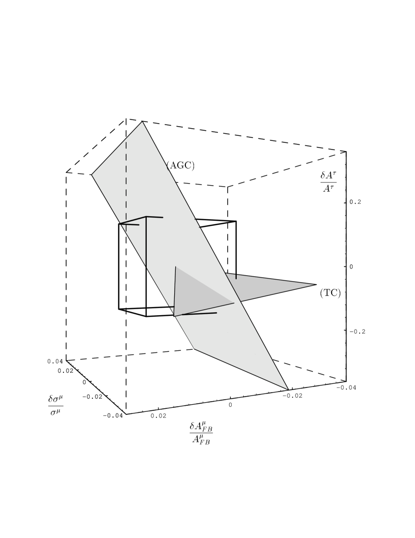
Figure 4: Trajectories in the 3-dimensional space of relative departures from SM for leptonic and hadronic observables $\sigma_{\mu}$, $A_{FB,\mu}$, $A_{\tau}$ at a LEP2 energy of 175 GeV for AGC models and TC models.
The box represents the unobservable domain corresponding to a relative accuracy of 1.5 percent for $\sigma_{\mu}$, $A_{FB,\mu}$ and 15 percent for $A_{\tau}$.

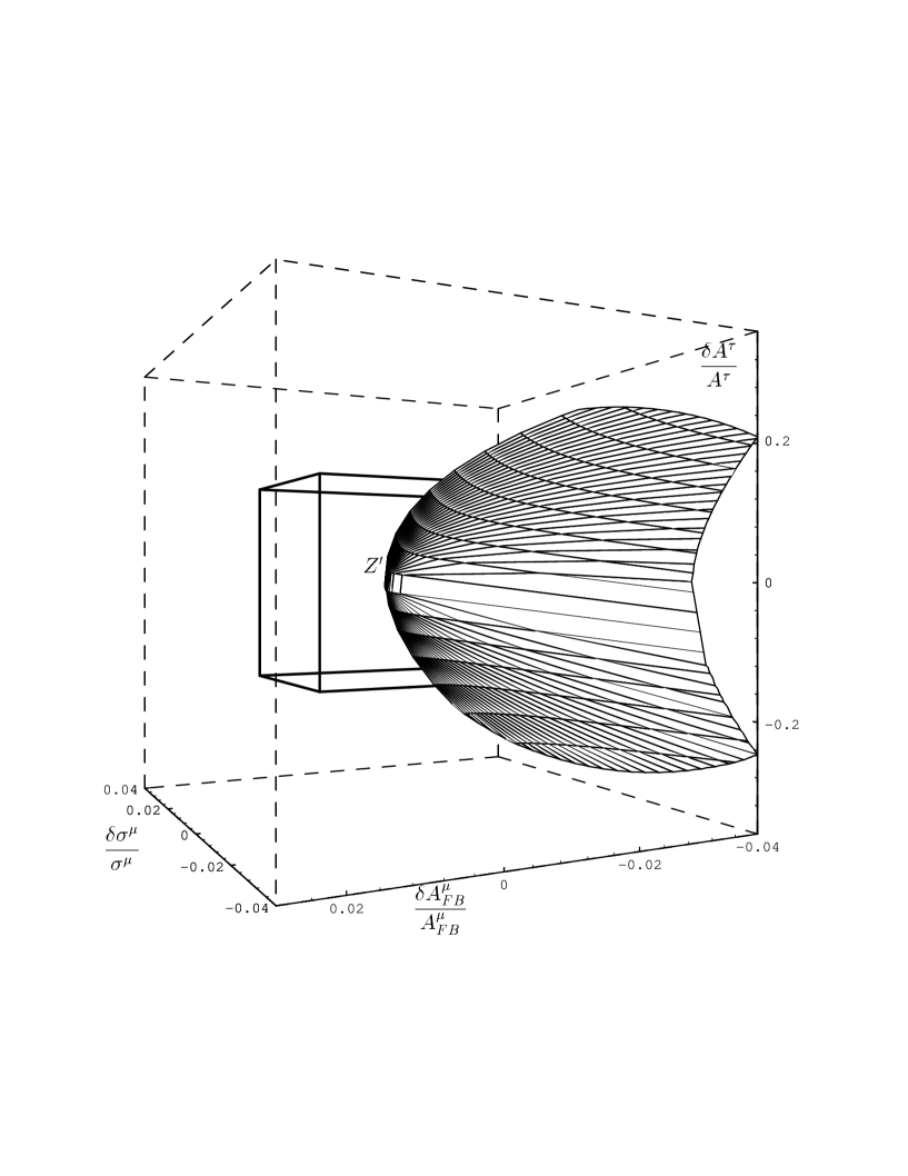
Figure 5: Trajectories in the 3-dimensional space of relative departures from SM for leptonic and hadronic observables $\sigma_{\mu}$, $A_{FB,\mu}$, $A_{\tau}$ at a LEP2 energy of 175 GeV for general $Z^{\prime}$ models.

As one sees, there is practically no overlapping in the meaningful region of the shifts space. This allows us to claim that, should a clear virtual effect manifest itself in the final lepton channel at LEP2, it would be possible to identify the responsible model within the limited (but reasonably representative) set of still surviving theoretical competitors. Our conclusions are obviously made possible by the fact that the number of involved parameters was reduced to two. Adding this final discussion to the results obtained in Section 3 we would therefore state, as claimed in the Introduction, that from our Z-peak subtracted approach a search of clean effects of a class of models with anomalous gauge couplings at future $e^{+}e^{-}$ colliders would, indeed, be made possible.

5 Conclusions

We have shown in this paper that a ”Z-peak subtracted” representation of four fermion (neutral current) processes allows to derive in a simple way realistic bounds for a reduced number of parameters of certain general models with Anomalous Gauge Couplings. The parameters that benefit from this approach are those that contribute the non constant part of the generalized self-energies $\tilde{F}_{i}(q^{2})$, $i=Z,\gamma Z,\gamma$. Other parameters are reabsorbed in the definition of various quantities measured on the $Z$ peak, that appear as new theoretical inputs replacing $G_{\mu}$.

This conclusion can be reexpressed in a way that represents sort of a compromise between previous discussions about the role of LEP1/SLC measurements with respect to LEP2 investigations [2], [3],[4],[5]. In our opinion, it is undeniable that a subset of the ”LEP1 blind” parameters of the model are also ”LEP2, NLC final-2-light fermion channel blind”. These are precisely those parameters that can be reabsorbed in $Z$-peak quantities, given their available experimental accuracy and given the realistic expected accuracy at LEP2, NLC. In the model that we have considered, these parameters are called $f_{BW}$ and $f_{\Phi,1}$. We cannot derive for their bounds any improvement when moving from LEP1/SLC to the LEP2 and NLC final light fermion channels. No direct information should also be expected on these parameters from the $WW$ channel. ${\cal O}_{\Phi,1}$ and $O_{DB}$ do not generate 3-gauge boson couplings ($O_{DW}$ and $O_{BW}$ do generate 3-boson couplings but due to the available LEP1 constraints they lie at an unobservable level in this channel). The $WW$ channel should only be fruitful for studying the blind operators $O_{WWW}$, $O_{W}$ and $O_{B}$.

The previous statements are supposed to be valid for a (neutral current) four fermion process. Here the Z-peak subtracted representation can be used. For other types of processes (like for instance charged current four fermion ones) this prescription cannot be utilized at least in the present formulation. In such cases, the conventional representation using $G_{\mu}$ can be used. An example of this type would be represented by a measurement of the W mass, whose theoretical expression depends also on the two parameters $f_{BW}$, $f_{\Phi,1}$ that cannot be reabsorbed in this case. In fact in our opinion, $M_{W}$ should be used in a separate fit to the AGC parameters together with the various Z-peak data and considered as another ”low energy input”.

One might imagine that further information on $f_{BW}$, $f_{\Phi,1}$ would be brought by the study of final $t\bar{t}$ states. Here, a priori, our subtraction technique cannot be applied so simply (because the necessary input $\Gamma_{Zt\bar{t}}$ does not exist). The fact is, though, that in this case a (probably) large number of extra $\simeq m^{2}_{t}$ parameters would appear (clearly in a not universal way), and the full analysis would become much more complicated.

To conclude this paper, we have considered the conventional analysis of ref.[6] where all the four parameters are retained. This comparison requires some care since the experimental picture and the computational details utilized there in the fit are not identical with ours. We can still remark that the bounds on $f_{DW}$, $f_{DB}$ are qualitatively consistent with ours. For the remaining two parameters, we see that, indeed, the relative improvement of ref.[6] from LEP2 to NLC is much weaker than that on the remaining two, in agreement with our expectations. There is an improvement from LEP1 to LEP2 for $f_{BW}$, $f_{\Phi,1}$ but this should be due, in our opinion, to the fact that the information from LEP2 contains also an assumed strongly improved measurement of $M_{W}$, which depends effectively, as we said, on $f_{BW}$, $f_{\Phi,1}$.

In principle, our approach could be generalized to models with a larger number of parameters. For instance, one might consider dimension eight operators in a model with AGC. Since those parameters that contribute the non constant component of the functions $F_{i}(q^{2})$ would survive, in a model like this with higher dimension operators there would certainly be several ones enjoying this property (e.g. of derivative type). Our statement is that our representation would free the various observables from spurious contributions from parameters like $f_{BW}$, $f_{\Phi,1}$ that could hide the determination of those parameters that are really effective at high energies, in particular those that would have a quartic increase $\simeq q^{4}/\Lambda^{4}$. With a sufficient number of experimental quantities a complete determination of the meaningful parameters might then be realistically achieved.

Acknowledgements: One of us (L.T.) acknowledge the hospitality received at the CERN TH division where a part of this work was carried out.

References

- [1] K.J.F. Gaemers and G.J. Gounaris, Z. Phys. (1979) 259; K. Hagiwara, R. Peccei, D. Zeppenfeld and K. Hikasa, Nucl. Phys. (1987) 253.
- [2] A. De Rújula, M.B. Gavela, P. Hernandez and E. Masso, Nucl. Phys. (1992) 3.
- [3] C. Grosse-Knetter, I. Kuss and D. Schildknecht, Z. Phys. (1993) 375.
- [4] M. Bilenky, J.L. Kneur, F.M. Renard and D. Schildknecht, Nucl. Phys. (1993) 22 and B419 (1994) 240.
- [5] K. Hagiwara, S. Ishihara, R. Szalapski and D. Zeppenfeld, Phys. Lett. (1992) 353 and Phys. Rev. (1993) 2182.
- [6] K. Hagiwara, S. Matsumoto and R. Szalapski, Phys. Lett. (1995) 411 .
- [7] F.M. Renard and C. Verzegnassi, Phys. Rev. (1995) 1369.
- [8] J. Layssac, F.M. Renard and C. Verzegnassi, Phys. Rev. (1994) 2143.
- [9] F.M. Renard and C. Verzegnassi, Phys. Rev. (1996) 1290.
- [10] Physics at LEP2, CERN 96-01, G. Altarelli, T. Sjostrand and F. Zwirner eds.
- [11] Collisions at 500 GeV: The Physics Potential, DESY 93-123C, p.345 (1993), P.M. Zerwas ed.
- [12] G. Degrassi and A. Sirlin, Nucl. Phys. (1992) 73 and Phys. Rev. (1992) 3104.
- [13] G. Altarelli, R. Barbieri, F. Caravaglios, Phys. Lett. (1993) 357 .
- [14] J. Layssac, F.M. Renard and C. Verzegnassi, Phys. Rev. (1994) 3650.
- [15] Z Physics at LEP1, CERN 89-08, Vol.1, p.203, G. Altarelli, R. Kleiss and C. Verzegnassi, eds.
- [16] For a review see also: O. Nicrosini and L. Trentadue, in Radiative Corrections for Collisions, J. H. Kühn, ed. (Springer, Berlin, 1989), p. 25; in QED Structure Functions, G. Bonvicini, ed., AIP Conf. Proc. No. 201 (AIP, New York, 1990), p. 12; O. Nicrosini, ibid., p. 73.
- [17] O. Nicrosini and L. Trentadue, Phys. Lett. (1987) 551 , Z. Phys. (1988) 479.
- [18] H. Burkhardt, F. Jegerlehner, G. Penso and C. Verzegnassi, Z. Phys. (1989) 497.
- [19] G. Montagna, O. Nicrosini, G. Passarino and F. Piccinini, “TOPAZ0 2.0 - A program for computing deconvoluted and realistic observables around the peak”, CERN-TH.7463/94, in press on Comput. Phys. Commun.; G. Montagna, O. Nicrosini, G. Passarino, F. Piccinini and R. Pittau, Comput. Phys. Commun. 76 (1993) 328.
- [20] This program is available, upon request, from the authors of this paper.