HD-THEP-96-13

hep-ph/9605283

September 9, 1996

EFFECTIVE THEORIES OF MSSM AT HIGH TEMPERATURE

M. Laine

Institut für Theoretische Physik, Philosophenweg 16, D-69120 Heidelberg, Germany

Abstract

We construct effective 3d field theories for the Minimal Supersymmetric Standard Model, relevant for the thermodynamics of the cosmological electroweak phase transition. The effective theories include a 3d theory for the bosonic sector of the original 4d theory; a 3d two Higgs doublet model; and a 3d SU(2)+Higgs model. The integrations are made at 1-loop level. In integrals related to vacuum renormalization we take into account only quarks and squarks of the third generation. Using existing non-perturbative lattice results for the 3d SU(2)+Higgs model, we then derive infrared safe upper bounds for the lightest Higgs boson mass required for successful baryogenesis at the electroweak scale. The Higgs mass bounds turn out to be close to those previously found with the effective potential, allowing baryogenesis if the right-handed stop mass parameter $m_{U}^{2}$ is small. Finally we discuss the effective theory relevant for $m_{U}^{2}$ very small, the most favourable case for baryogenesis.

1 Introduction

The generation of the baryon number of the Universe remains to be satisfactorily explained. It is quite plausible, though, that an important role in the process was played by the cosmological electroweak phase transition [1]. Within the Standard Model the phase transition appears nevertheless to be too weakly of first order to produce the baryon asymmetry for realistic Higgs masses (for a review, see [2]). Additional problems may be related to the amount of CP-violation available. Hence one is led to extensions of the Standard Model.

One possible consistent extension of the Standard Model is the Minimal Supersymmetric Standard Model (MSSM). It has a large parameter space available so that it should be possible to find some corner with a strong enough first order transition. In addition, there are additional sources of CP-violation. Indeed, the electroweak phase transition in MSSM has been studied quite actively [3–7].

The investigations made so far (apart from [38, 39]) have been based on the 1- and 2-loop effective potentials for the Higgs field. The limit that the CP-odd Higgs mass $m_{A}$ is infinite was taken in [3, 4, 6, 7], leaving just one Higgs doublet and being the most favourable case for baryogenesis [5]. The result of these investigations was that in general, it appears difficult to make a strong enough transition unless the right-handed soft supersymmetry breaking stop mass parameter $m_{U}^{2}$ is small. Recently it has been noted that even smaller values of $m_{U}^{2}$ than originally considered should be phenomenologically possible [6], leading to a transition that is definitely strong enough for baryogenesis. In addition, 2-loop effects have been found to be favourable [7].

All the studies based on the effective potential are subject to the infrared (IR) problem at finite temperature [8]. The IR problem is related to the zero Matsubara components of bosonic fields, and precisely these components account for the cubic 1-loop terms in the effective potential studied in [3–6], as well as for the logarithmic 2-loop terms making the effect in [7]. The IR-problem calls for non-perturbative investigations of the problem. The method of choice for non-perturbative investigations is the framework of dimensional reduction [9–17]. Dimensional reduction means that one constructs an effective 3d theory producing the same Green’s functions as the original theory for the light bosonic fields. The perturbative dimensional reduction step is free of IR-problems, and the resulting super-renormalizable 3d theory can then be studied with high precision Monte Carlo simulations [18–22].

The non-perturbative investigations of the electroweak phase transition in the Standard Model have revealed the following pattern [19]. As long as the transition is strong enough for baryogenesis, the IR-problems are not very dramatic and effective potential studies do produce a reasonable estimate of the properties of the phase transition. When the transition gets weaker, non-perturbative effects become large. However, even if non-perturbative effects are small for stronger transitions, it is nevertheless interesting to note that prior to the lattice study in [19] many perturbative studies stated that baryogenesis was possible up to $m_{H}\sim 45$ GeV. In [19] it was discovered that practically no Higgs mass is possible. While this effect is mostly related to vacuum renormalization instead of non-perturbative IR-effects, it nevertheless proves that it is important to work in a consistent framework where all the approximations are under control.

The purpose of the present paper is to make a dimensional reduction for the MSSM. We also perform further integrations inside the dimensionally reduced 3d theory, to arrive at the simplest possible effective theory. In particular, we construct a 3d two Higgs doublet model and a 3d SU(2)+Higgs model in the part of the parameter space where it is possible. For the latter theory, the existing non-perturbative lattice results allow to remove the IR problem from the Higgs mass bound. The bound derived is in principle also gauge and $\bar{\mu}$-independent, unlike the ratio $v(T_{c})/T_{c}$ derived from the effective potential.

On the technical side, one purpose of the present investigation is to study how the cubic scalar vertices, not present in the Standard Model, affect dimensional reduction.

In comparison with [4–7], we also try to be more explicit about the effects of vacuum renormalization. The theory studied is more or less the same. We include here the bottom Yukawa coupling $h_{b}$ and study a general CP-odd Higgs mass $m_{A}$ as in [5].

It is found that in the region of the parameter space where reduction into the 3d SU(2)+Higgs model is possible and the transition is strong enough for baryogenesis, the non-perturbative results agree with the effective potential investigations. The conclusion is that Higgs masses $m_{h}\raise 1.29167pt\hbox{$<$\kern-7.5pt\raise-4.73611pt\hbox{$\sim$}}75$ GeV produce a strong enough transition if $m_{U}^{2}$ is small enough, $m_{U}^{2}\raise 1.29167pt\hbox{$<$\kern-7.5pt\raise-4.73611pt\hbox{$\sim$}}(50-100)^{2}$ GeV². Hence, the situation has improved with respect to the Standard Model where no Higgs mass is possible. Where reduction into SU(2)+Higgs cannot be made — notably when $m_{U}^{2}$ is still smaller and the transition is even stronger [6, 7] — we propose an effective 3d theory allowing more detailed studies of the problem.

The plan of the paper is the following. In Sec. 2 we briefly review the Higgs mass bound in the Standard Model and its derivation within the 3d framework. In Sec. 3 we state in some detail the approximations adopted and the Lagrangian used in the present investigation. Sec. 4 contains the dimensional reduction into a 3d bosonic effective theory. In Sec. 5 we make further integrations inside the 3d theory, removing the squarks and the temporal components of the gauge fields. The resulting two Higgs doublet model is diagonalized in Sec. 6, and the heavy Higgs doublet in integrated out in Sec. 7. In Sec. 8 we discuss how the running Lagrangian parameters are fixed through vacuum renormalization. The numerical results for the strength of the transition are in Sec. 9. Finally, in Sec. 10 we propose an effective theory for describing the phase transition if the mass parameter $m_{U}^{2}$ is very small. Sec. 11 is the conclusions.

2 The EW phase transition in the Standard Model

The thermodynamics of the electroweak phase transition in the full Standard Model has been extensively studied in the literature ([2] and references therein). Perturbative studies exist up to 2-loop level [23, 24, 14, 25]. Non-perturbative lattice studies rely on perturbative 2-loop dimensional reduction [12–15], and have been performed for a wide range of Higgs masses [18–22]. The Higgs mass bound in terms of the parameters of the 3d SU(2)+Higgs model was derived in [19].

The Higgs mass bound arises as follows. Assume that there in some underlying physical 4d theory in which the electroweak phase transition takes place so that the static Green’s functions of the lightest excitations are described by the effective theory

$$L_{\rm 3d} = {\frac{1}{4}}F^{a}_{ij}F^{a}_{ij}+(D_{i}\phi)^{\dagger}(D_{i}\phi)+m_{3}^{2}\phi^{\dagger}\phi+\lambda_{3}(\phi^{\dagger}\phi)^{2},$$ (2.1)

where $D_{i}=\partial_{i}-ig_{3}\tau^{a}A^{a}_{i}/2$. Then the phase transition is strong enough for baryogenesis if at the phase transition point [19]

$$x\equiv\frac{\lambda_{3}}{g_{3}^{2}}<0.03-0.04.$$ (2.2)

Since the theory in eq. (2.1) is super-renormalizable, the parameters $\lambda_{3},g_{3}^{2}$ do not run and the quantity $x$ is a well-defined pure number. It is also gauge-independent. The uncertainty in (2.2) arises from uncertainties in estimates of the sphaleron rate in the broken phase and from uncertainties in the real-time dynamics of the phase transition (whether the Universe reheats back to $T_{c}$ after the nucleation period, etc.).

For the Standard Model, the parameters $m_{3}^{2}$, $\lambda_{3}$ and $g_{3}^{2}$ have been calculated in terms of temperature and the physical zero-temperature parameters of the theory in [15]. Then one may solve for the critical temperature from the condition

$$m_{3}^{2}(m_{h},T_{c})=0,$$ (2.3)

and use this $T_{c}$ in the estimate of

$$x=\frac{\lambda_{3}(m_{h},T_{c})}{g_{3}^{2}(m_{h},T_{c})}.$$ (2.4)

Eq. (2.3) does not give $T_{c}$ exactly (it corresponds to resummed 1-loop accuracy), but this does not matter since $\lambda_{3}/g_{3}^{2}$ depends on $T_{c}$ only through logarithmic 1-loop corrections. From an analysis of the type outlined, one gets that no Higgs mass (or at most an extremely light Higgs mass, $m_{h}\raise 1.29167pt\hbox{$<$\kern-7.5pt\raise-4.73611pt\hbox{$\sim$}}20$ GeV) would satisfy the bound (2.2) in the Standard Model since $x>0.04$ due to top Yukawa coupling corrections, see Fig. 27 in [19].

In this paper we study whether a theory of the type in eq. (2.1) can be constructed in the MSSM and what would be the Higgs mass bound implied.

3 The Lagrangian

We start by discussing the Lagrangian used and the simplifications made, fixing at the same time the notation. We work throughout in Euclidian space and for definiteness in the Landau gauge. The value of $x$ derived is gauge-independent.

The main simplifications are the following (for the complete Lagrangian in MSSM, see [26]). First, we neglect the U(1) subgroup in loop corrections related to vacuum renormalization and dimensional reduction. That is, no difference is made between $g^{2}$ and $g^{2}+g^{\prime 2}$ beyond tree-level in IR-safe integrals. This is a good approximation as far as the electroweak phase transition is concerned, especially with respect to the other uncertainties in the calculation. Even at tree-level, we display explicitly only the covariant derivatives related to SU(2) and SU(3).

Second, we will assume that the gaugino and higgsino mass parameters in the symmetric phase are so large that these fields have decoupled, as is usually assumed in the present context [4–7]. Even if the masses are smaller, these fields do not have very much significance, being fermions: at finite temperature, the important effects arise from IR-sensitive bosons. In the framework of the present paper, the extra fermions would only affect the parameters of the 3d theory in the first dimensional reduction step, but the later integrations remain precisely the same. It should also be noted that gauginos and higgsinos do not couple to the scalar Higgs degrees of freedom through the dominant Yukawa coupling $h_{t}$, unlike the top quark. In general, it is expected that the effect of gauginos and higgsinos would be to make the phase transition weaker, due to the increased screening in the thermal masses [4, 5, 7]. However, gauginos and higgsinos do have an effect when 1-loop corrections to the top Yukawa coupling $h_{t}$ are calculated. Since $h_{t}$ gives the most important effects in the present calculation, the loop corrections may also be important. We return to this point in more detail below.

Third, only the squark partners of top and bottom quarks are assumed to be light enough to affect the electroweak phase transition.

Then the remaining fields are as follows: there are the SU(2) and SU(3) gauge fields $A^{a}_{\mu}$, $C^{A}_{\mu}$. The Higgs fields are $H^{1},H^{2}$, with hypercharges $Y=-1,+1$. The adjoint Higgs fields with opposite hypercharges are denoted by

$$\tilde{H}^{1}=i\tau_{2}H^{1*},\quad\tilde{H}^{2}=i\tau_{2}H^{2*}.$$ (3.1)

The 2-index antisymmetric tensor is defined through $\epsilon_{12}=-1$, so that $\tilde{H}^{n}_{i}=-\epsilon_{ij}H^{n*}_{j}$. We use the notation

$$H^{1}=\left(\begin{array}[]{l}H^{1}_{1}\\ H^{1}_{2}\end{array}\right)=\frac{1}{\sqrt{2}}\left(\begin{array}[]{r}h^{1}_{0}+ih^{1}_{3}\\ -h^{1}_{2}+ih^{1}_{1}\end{array}\right),\quad H^{2}=\left(\begin{array}[]{l}H^{2}_{1}\\ H^{2}_{2}\end{array}\right)=\frac{1}{\sqrt{2}}\left(\begin{array}[]{l}h^{2}_{2}+ih^{2}_{1}\\ h^{2}_{0}-ih^{2}_{3}\end{array}\right)$$ (3.2)

for the complex and real components of the Higgs fields, so that at zero temperature

$$\langle h^{1}_{0}\rangle=v_{1},\quad\langle h^{2}_{0}\rangle=v_{2}.$$ (3.3)

The fermions of the third generation are

$$q_{L\alpha}=\left(\begin{array}[]{l}t_{L\alpha}\\ b_{L\alpha}\end{array}\right),\quad t_{R\alpha},\quad b_{R\alpha},$$ (3.4)

where $\alpha$ is the SU(3)-index and the hypercharges are $Y=1/3,4/3,-2/3$, respectively. Correspondingly, the squarks of the third generation are

$$Q_{\alpha}=\left(\begin{array}[]{l}\tilde{t}_{L\alpha}\\ \tilde{b}_{L\alpha}\end{array}\right),\quad\quad U_{\alpha}=\tilde{t}_{R\alpha}^{*},\quad D_{\alpha}=\tilde{b}_{R\alpha}^{*},$$ (3.5)

with the hypercharges $Y=1/3,-4/3,2/3$. The fields $U,D$ transform under SU(3) with the adjoint generators $\overline{\lambda}_{A}=-\lambda_{A}^{*}$.

The part of the action containing the kinetic terms of and interactions between gauge fields and fermions remains as in the Standard Model. For the Higgs and squark fields the quadratic terms are

$$L = (D^{w}_{\mu}H^{1})^{\dagger}(D^{w}_{\mu}H^{1})+(D^{w}_{\mu}H^{2})^{\dagger}(D^{w}_{\mu}H^{2})$$ (3.6)

$$+ m_{1}^{2}H^{1\dagger}H^{1}+m_{2}^{2}H^{2\dagger}H^{2}+m_{12}^{2}(H^{1\dagger}\tilde{H}^{2}+\tilde{H}^{2\dagger}H^{1})$$

$$+ (D^{ws}_{\mu}Q)^{\dagger}(D^{ws}_{\mu}Q)+(D^{s}_{\mu}U^{*})^{\dagger}(D^{s}_{\mu}U^{*})+(D^{s}_{\mu}D^{*})^{\dagger}(D^{s}_{\mu}D^{*})$$

$$+ m_{Q}^{2}Q_{\alpha}^{\dagger}Q_{\alpha}+m_{U}^{2}U_{\alpha}^{*}U_{\alpha}+m_{D}^{2}D_{\alpha}^{*}D_{\alpha},$$

where $D_{\mu}^{ws}=\partial_{\mu}-ig\tau^{a}A^{a}_{\mu}/2-ig_{S}\lambda^{A}C^{A}_{\mu}/2$ and $w$ and $s$ indicate the charge included.

The supersymmetric interactions are generated by the superpotential and by the $D$-terms. We take the superpotential to be

$$W=\mu\epsilon_{ij}H^{1}_{i}H^{2}_{j}+h_{t}\epsilon_{ij}H^{2}_{i}Q_{j\alpha}U_{\alpha}+h_{b}\epsilon_{ij}H^{1}_{i}Q_{j\alpha}D_{\alpha}.$$ (3.7)

Hence also the bottom Yukawa coupling $h_{b}$ is kept, although its effect is small since the region of parameter space which can affect baryogenesis is around $\tan\!\beta=v_{2}/v_{1}\sim 2$, and $h_{b}\sim m_{b}/(2m_{Z}\cos\beta)$. The interaction Lagrangian following from the superpotential is

$$L_{W} = h_{t}\Bigl{(}\bar{t}_{R}\tilde{H}^{2\dagger}q_{L}+\bar{q}_{L}\tilde{H}^{2}t_{R}\Bigl{)}+h_{b}\Bigl{(}\bar{b}_{R}\tilde{H}^{1\dagger}q_{L}+\bar{q}_{L}\tilde{H}^{1}b_{R}\Bigl{)}$$ (3.8)

$$+ h_{t}^{2}\Bigl{(}Q^{*}_{i\alpha}U^{*}_{\alpha}Q_{i\beta}U_{\beta}+H^{2\dagger}H^{2}U^{*}_{\alpha}U_{\alpha}+\tilde{H}^{2\dagger}Q_{\alpha}Q^{\dagger}_{\alpha}\tilde{H}^{2}\Bigr{)}$$

$$+ h_{b}^{2}\Bigl{(}Q^{*}_{i\alpha}D^{*}_{\alpha}Q_{i\beta}D_{\beta}+H^{1\dagger}H^{1}D^{*}_{\alpha}D_{\alpha}+\tilde{H}^{1\dagger}Q_{\alpha}Q^{\dagger}_{\alpha}\tilde{H}^{1}\Bigr{)}$$

$$+ h_{t}h_{b}\Bigl{(}H^{2\dagger}H^{1}U^{*}_{\alpha}D_{\alpha}+H^{1\dagger}H^{2}U_{\alpha}D^{*}_{\alpha}\Bigr{)}.$$

The interaction Lagrangian following from the $D$-terms, on the other hand, is

$$L_{D} = \frac{g^{\prime 2}}{8}\Bigl{[}H^{1\dagger}H^{1}-H^{2\dagger}H^{2}\Bigr{]}^{2}$$ (3.9)

$$+ \frac{g^{2}}{8}\Bigl{[}Q^{*}_{i\alpha}Q_{j\alpha}+H^{m*}_{i}H^{m}_{j}\Bigr{]}\Bigl{[}Q^{*}_{k\beta}Q_{l\beta}+H^{n*}_{k}H^{n}_{l}\Bigr{]}\tau^{a}_{ij}\tau^{a}_{kl}$$

$$+ \frac{g_{S}^{2}}{8}\Bigl{[}Q^{*}_{i\alpha}Q_{i\beta}-U_{\alpha}U^{*}_{\beta}-D_{\alpha}D^{*}_{\beta}\Bigr{]}\Bigl{[}Q^{*}_{j\gamma}Q_{j\delta}-U_{\gamma}U^{*}_{\delta}-D_{\gamma}D^{*}_{\delta}\Bigr{]}\lambda^{A}_{\alpha\beta}\lambda^{A}_{\gamma\delta}.$$

Here we kept the U(1) coupling $g^{\prime}$ only in the Higgs sector. In eq. (3.9),

$$\tau^{a}_{ij}\tau^{a}_{kl}=(2\delta_{il}\delta_{jk}-\delta_{ij}\delta_{kl}),\quad\lambda^{A}_{\alpha\beta}\lambda^{A}_{\gamma\delta}={\frac{2}{3}}(3\delta_{\alpha\delta}\delta_{\beta\gamma}-\delta_{\alpha\beta}\delta_{\gamma\delta}).$$ (3.10)

The soft supersymmetry breaking cubic interactions are

$$L=u_{s}\tilde{H}^{2\dagger}Q_{\alpha}U_{\alpha}+d_{s}\tilde{H}^{1\dagger}Q_{\alpha}D_{\alpha}+e_{s}H^{2\dagger}Q_{\alpha}D_{\alpha}+w_{s}H^{1\dagger}Q_{\alpha}U_{\alpha}+{\rm H.c.}$$ (3.11)

Here we use the notation of [26], with opposite signs. The relation to the more standard $A$-parameters is discussed in Sec. 8 in connection with vacuum renormalization. In particular, it should be noted that the parameter $e_{s}$ includes the term $\mu h_{b}$ arising from the superpotential and the parameter $w_{s}$ includes $-\mu h_{t}$. Since there is also an arbitrary soft component in these terms [26] and since we assume the higgsinos to be so heavy that they have decoupled, the theory does in fact not depend at all on the true supersymmetric mass parameter $\mu$. In the following, we shall restrict the parameters $u_{s},d_{s},e_{s},w_{s}$ to be real.

Although quite a few simplifications have been made, there are still a lot more parameters left than in the Standard Model. The two scalar sector parameters $\nu^{2},\lambda$ appearing there are replaced by $m_{1}^{2},m_{2}^{2},m_{12}^{2},m_{Q}^{2},m_{U}^{2},m_{D}^{2},u_{s},d_{s},e_{s},w_{s}$.

There is the following important point to be noticed about the coupling constants $g,g_{S},h_{t},h_{b}$ in the present theory. As an example, take the gauge coupling. If one takes the theory under investigation as such, then the weak gauge coupling in the gauge sector runs as

$$\bar{\mu}\frac{dg^{2}(\bar{\mu})}{d\bar{\mu}}=\frac{g^{4}}{8\pi^{2}}\frac{8n_{F}+N_{s}-44}{6},$$ (3.12)

where $n_{F}=3$ is the number of families and $N_{s}=5$ is the number of scalar doublets interacting with the SU(2) gauge fields. However, the couplings $g_{1}^{2},g_{2}^{2},g_{3}^{2},g_{4}^{2}=g^{2}$ in the SU(2)-part of the scalar potential following from eq. (3.9),

$$V={\frac{1}{8}}g_{1}^{2}({H^{1}}^{\dagger}H^{1})^{2}+{\frac{1}{8}}g_{2}^{2}({H^{2}}^{\dagger}H^{2})^{2}+{\frac{1}{4}}g_{3}^{2}{H^{1}}^{\dagger}H^{1}{H^{2}}^{\dagger}H^{2}-{\frac{1}{2}}g_{4}^{2}{H^{1}}^{\dagger}\tilde{H}^{2}\tilde{H}^{2\dagger}H^{1},$$ (3.13)

run as

$$\bar{\mu}\frac{dg_{1}^{2}(\bar{\mu})}{d\bar{\mu}} = \bar{\mu}\frac{dg_{2}^{2}(\bar{\mu})}{d\bar{\mu}}=\bar{\mu}\frac{dg_{3}^{2}(\bar{\mu})}{d\bar{\mu}}=\frac{7}{2}\frac{g^{4}}{8\pi^{2}},$$ (3.14)

$$\bar{\mu}\frac{dg_{4}^{2}(\bar{\mu})}{d\bar{\mu}} = -\frac{5}{2}\frac{g^{4}}{8\pi^{2}}.$$ (3.15)

Hence within the present theory one would have to renormalize these couplings separately from the coupling in the gauge sector. In other words, one has to consider a large number of zero-temperature observables in terms of which to fix the independent parameters. If on the other hand one wants to maintain the universality of the gauge coupling, then one has to include the complete supersymmetric structure of the theory in the calculation in one way or the other. In the present theory, supersymmetry is maintained only in the quark-squark sector of the third generation, and indeed, if only these fields are included in the internal lines of loop integrals, then $g^{2}$ runs everywhere as

$$\bar{\mu}\frac{dg^{2}(\bar{\mu})}{d\bar{\mu}}=\frac{3}{2}\frac{g^{4}}{8\pi^{2}}$$ (3.16)

We shall work within the accuracy of this approximation here and assume the gauge coupling to be universal.

The same thing applies also to the Yukawa couplings $h_{t},h_{b}$ and is quite important there as well, since $h_{t}$ is large and gives the dominant effects. Indeed, within the present theory, the Yukawa couplings in the different squark-Higgs and quark-Higgs interactions run differently. To get a universal Yukawa coupling, higgsinos and gauginos should be included. However, we will be satisfied with the present approximation in this paper for two reasons. First, the Yukawa coupling $h_{t}$ is determined by the top mass which is not known very precisely at the moment. Second and even more important, the most significant effects of $h_{t}$ appear in conjunction with the soft squark mass parameters $m_{Q}^{2},m_{U}^{2},m_{D}^{2}$ (see below). Since these are unknown, there is a large uncertainty in the calculation in any case. Once the squark masses have been measured and the top mass is known more precisely, the gauge coupling $h_{t}(\bar{\mu})$ should be fixed at 1-loop level in terms of the top pole mass.

We will work in the $\overline{\mbox{\rm MS}}$ scheme (with the scale parameter $\bar{\mu}$) and take ${\rm Tr\,}1=4$. For the squark and quark loops included in vacuum renormalization the results agree with those in the $\overline{\mbox{\rm DR}}$-scheme, often used in supersymmetric theories.

4 Dimensional reduction

Let us first recall the expansion parameters of dimensional reduction [15]. Since all the calculations are IR-safe, no non-analytic powers of masses can appear. In fact, the expansion proceeds just in powers of

$$\frac{h_{t}^{2}}{16\pi^{2}},\quad\frac{g_{S}^{2}}{16\pi^{2}}$$ (4.1)

as at zero temperature. We include only the quarks and squarks of the third generation in the loops affecting vacuum renormalization, whereas the corrections e.g. from gauge bosons, suppressed by $g^{2}/(16\pi^{2})$, are neglected.

In addition to expanding in coupling constants, we make a high-temperature expansion in the mass parameters. This requires that the soft supersymmetry breaking mass parameters satisfy

$$m_{1}^{2},m_{2}^{2},m_{12}^{2},m_{U}^{2},m_{D}^{2},m_{Q}^{2}<(2\pi T_{c})^{2}.$$ (4.2)

The limit (4.2) implies that $m_{A}\raise 1.29167pt\hbox{$<$\kern-7.5pt\raise-4.73611pt\hbox{$\sim$}}2\pi T_{c}$, so that the results of this paper cannot be directly continued to the limit $m_{A}\to\infty$ studied in [4, 6, 7]. Actually, the limitation on $m_{A}$ is not as important as that on the squark mass parameters, since the latter are associated with larger coupling constants.

To keep track of the validity of the high-temperature expansion, we will at some points display also the leading correction terms. The critical temperature is $T_{c}\sim 100$ GeV so that we shall assume $m_{Q},m_{U},m_{D},m_{A}\raise 1.29167pt\hbox{$<$\kern-7.5pt\raise-4.73611pt\hbox{$\sim$}}300$ GeV. We also assume that the masses generated at the electroweak phase transition as well as the masses associated with possible colour and charge breaking minima are small compared with $2\pi T_{c}$.

If some of the soft masses are large, one cannot use the high-temperature expansion. Instead, one should evaluate the corresponding integrals numerically. If $m\gg 2\pi T_{c}$, one can also integrate out these degrees of freedom in the sense of the vacuum decoupling theorem [27].

The actual dimensional reduction proceeds by writing down the general form of the effective 3d theory and then determining the 3d coupling constants by matching the Green’s functions in the original theory and in the 3d theory. The degrees of freedom of the effective theory are the bosonic degrees of freedom of the original theory. The temporal components of gauge fields become Higgs fields in the adjoint representation. The structure of the 3d theory is determined by gauge invariance. The 1-loop calculations needed are a straightforward application of the rules in [15]. We just write down the graphs and the results below.

Since the complete bosonic sector of MSSM is rather large, we display only the part interacting with the SU(2) and Higgs degrees of freedom explicitly. We recall that after trivial rescaling with $T$, the dimension of bosonic fields in 3d is GeV^1/2 and that of the couplings $g_{3}^{2},g_{3}^{\prime 2},h_{t3}^{2},h_{b3}^{2}$ is GeV. At some points, we denote new parameters with the same symbols as the old ones, to avoid increasingly cumbersome notation. Higher-order operators suppressed by the temperature and coupling constants are neglected. Finally, let us recall some basic notation:

$$c_{B} = \ln(4\pi)-\gamma_{E}\approx 1.953808,\quad c_{F}=c_{B}-2\ln 2\approx 0.567514,$$ (4.3)

$$L_{b}(\bar{\mu}) = 2\ln\frac{\bar{\mu}}{T}-2c_{B},\quad L_{f}(\bar{\mu})=2\ln\frac{\bar{\mu}}{T}-2c_{F}.$$ (4.4)

The 3d effective theory consists of the following parts:

1. The temporal components of the original gauge fields become scalar fields in the adjoint representation, and the spatial components remain gauge fields. Relevant for the present discussion is the part

$$L_{\rm gauge}={\frac{1}{4}}F^{a}_{ij}F^{a}_{ij}+{\frac{1}{2}}(D_{i}A_{0}^{a})^{2}+{\frac{1}{2}}m_{A_{0}}^{2}A_{0}^{a}A_{0}^{a}+{\frac{1}{2}}(\partial_{i}C_{0}^{A})^{2}+{\frac{1}{2}}m_{C_{0}}^{2}C_{0}^{A}C_{0}^{A},$$ (4.5)

where $D_{i}A_{0}^{a}=\partial_{i}A_{0}^{a}+g_{3}\epsilon^{abc}A^{b}_{i}A^{c}_{0}$. When only quarks and squarks are included, the 3d fields are related to the renormalized 4d fields by

$$(A_{0}^{a}A_{0}^{b})^{({\rm new})} = \frac{1}{T}(A_{0}^{a}A_{0}^{b})(\bar{\mu})\biggl{[}1+\frac{g^{2}}{16\pi^{2}}\biggl{(}[L_{f}(\bar{\mu})-1]+{\frac{1}{2}}[L_{b}(\bar{\mu})+2]\biggr{)}\biggr{]},$$ (4.6)

$$(A_{i}^{a}A_{j}^{b})^{({\rm new})} = \frac{1}{T}(A_{i}^{a}A_{j}^{b})(\bar{\mu})\biggl{[}1+\frac{g^{2}}{16\pi^{2}}\biggl{(}L_{f}(\bar{\mu})+{\frac{1}{2}}L_{b}(\bar{\mu})\biggr{)}\biggr{]},$$ (4.7)

where mass corrections suppressed by $m_{Q}^{2}/(2\pi T_{c})^{2}$ were neglected.

The gauge coupling can be most easily obtained from the graphs (qqqq), (SS), (SSS1), (SSS2), (SSSS) in Fig. 1.c. Here also a redefinition of the Higgs fields, given in (4.12)–(4.13), is needed. After the redefinition one gets

$$g_{3}^{2}=g^{2}(\bar{\mu})T\biggl{[}1-\frac{g^{2}}{16\pi^{2}}\biggl{(}L_{f}(\bar{\mu})+{\frac{1}{2}}L_{b}(\bar{\mu})\biggr{)}\biggr{]},$$ (4.8)

so that $g_{3}^{2}(A_{i}^{a}A_{j}^{b})^{({\rm new})}=g^{2}A^{a}_{i}A^{b}_{j}$.

The values of $m_{A_{0}}^{2},m_{C_{0}}^{2}$ are well known [5, 7], but for completeness we write them here as well. These terms contain only screening parts not related to vacuum renormalization, so that we include the complete spectrum of the model in the loops. With the notation in Fig. 1.a, the graphs contributing to $m_{A_{0}}$ are (ff), (gg), (AA), (HH), (QQ), (A), (H), (Q); to $m_{C_{0}}$ contribute (ff), (gg), (CC), (SS), (C), (S). For illustration, the leading mass terms are also shown:

$$m_{A_{0}}^{2} = g^{2}\biggl{[}\biggl{(}{\frac{2}{3}}+\frac{n_{F}=3}{3}+\frac{N_{s}=5}{6}\biggr{)}T^{2}+\frac{1}{8\pi^{2}}(m_{1}^{2}+m_{2}^{2}+3m_{Q}^{2})\biggr{]},$$ (4.9)

$$m_{C_{0}}^{2} = g_{S}^{2}\biggl{[}\biggl{(}1+\frac{n_{F}=3}{3}+\frac{N_{s}=4}{6}\biggr{)}T^{2}+\frac{1}{8\pi^{2}}(m_{U}^{2}+m_{D}^{2}+2m_{Q}^{2})\biggr{]}.$$ (4.10)

In eqs. (4.9), (4.10), $n_{F}=3$ is the number of fermion families and $N_{s}$ is the number of scalar doublets interacting with the gauge fields in question.

Figure 1: The generic types of graphs needed for dimensional reduction of (a) wave functions and masses, (b) scalar couplings and (c) the gauge coupling. Wiggly lines are vector propagators and dashed lines represent generic propagators of particle type P$=$Q, U, D, S, H, A, C, g, q, f. Here Q, U, D denote the corresponding squarks, S is a squark in general, H is a Higgs doublet, A and C are the SU(2) and SU(3) gauge fields, g is a ghost, q a third generation quark and f a general fermion. For the coupling constants, 1-loop dimensional reduction is directly related to 1-loop vacuum renormalization and hence only squarks and quarks are considered in the internal lines. For the masses, the thermal screening terms proportional to $T^{2}$ are not related to vacuum renormalization and hence we include all the modes with $m\raise 1.29167pt\hbox{$<$\kern-7.5pt\raise-4.73611pt\hbox{$\sim$}}2\pi T$ in the loops.

2. The quadratic terms of the Higgs sector are

$$L_{\rm Higgs} = (D_{i}H^{1})^{\dagger}(D_{i}H^{1})+(D_{i}H^{2})^{\dagger}(D_{i}H^{2})+\xi\Bigl{[}(D_{i}H^{1})^{\dagger}(D_{i}\tilde{H}^{2})+{\rm H.c.}\Bigr{]}$$ (4.11)

$$+ m_{1}^{2}H^{1\dagger}H^{1}+m_{2}^{2}H^{2\dagger}H^{2}+m_{12}^{2}(H^{1\dagger}\tilde{H}^{2}+\tilde{H}^{2\dagger}H^{1}),$$

where $D_{i}=\partial_{i}-ig_{3}\tau^{a}A^{a}_{i}/2$ and $g_{3}$ is the 3d gauge coupling. The graphs contributing to the 2-point Higgs correlators are (qq), (AH), (SS), (A), (H), (S) in Fig. 1.a. According to the general strategy of including only quark and squark loops in terms related to vacuum renormalization, we neglect terms multiplied by $g^{2}$ everywhere except for the screening parts proportional to $T^{2}$. The new fields are then related to the renormalized 4d fields in the $\overline{\mbox{\rm MS}}$ scheme by

$$(H^{1\dagger}H^{1})^{({\rm new})} = \frac{1}{T}(H^{1\dagger}H^{1})(\bar{\mu})\biggl{[}1+\frac{1}{16\pi^{2}}3h_{b}^{2}L_{f}(\bar{\mu})+\frac{\zeta(3)}{128\pi^{4}}\frac{d_{s}^{2}+w_{s}^{2}}{T^{2}}\biggr{]},$$ (4.12)

$$(H^{2\dagger}H^{2})^{({\rm new})} = \frac{1}{T}(H^{2\dagger}H^{2})(\bar{\mu})\biggl{[}1+\frac{1}{16\pi^{2}}3h_{t}^{2}L_{f}(\bar{\mu})+\frac{\zeta(3)}{128\pi^{4}}\frac{u_{s}^{2}+e_{s}^{2}}{T^{2}}\biggr{]}.$$ (4.13)

The mass parameters, on the other hand, are

$${m_{1}^{2}}^{({\rm new})} = m_{1}^{2}(\bar{\mu})-\frac{3}{16\pi^{2}}\Bigl{[}h_{b}^{2}(m_{Q}^{2}+m_{D}^{2})L_{b}(\bar{\mu})+h_{b}^{2}m_{1}^{2}L_{f}(\bar{\mu})+(d_{s}^{2}+w_{s}^{2})L_{b}(\bar{\mu})\Bigr{]}$$ (4.14)

$$+ \biggl{(}{\frac{3}{4}}h_{b}^{2}+{\frac{1}{4}}g^{2}\biggr{)}T^{2}$$

$$+ \frac{\zeta(3)}{128\pi^{4}T^{2}}\Bigl{[}3d_{s}^{2}(m_{Q}^{2}+m_{D}^{2})+3w_{s}^{2}(m_{Q}^{2}+m_{U}^{2})-(d_{s}^{2}+w_{s}^{2})m_{1}^{2}\Bigr{]},$$

$${m_{2}^{2}}^{({\rm new})} = m_{2}^{2}(\bar{\mu})-\frac{3}{16\pi^{2}}\Bigl{[}h_{t}^{2}(m_{Q}^{2}+m_{U}^{2})L_{b}(\bar{\mu})+h_{t}^{2}m_{2}^{2}L_{f}(\bar{\mu})+(u_{s}^{2}+e_{s}^{2})L_{b}(\bar{\mu})\Bigr{]}$$ (4.15)

$$+ \biggl{(}{\frac{3}{4}}h_{t}^{2}+{\frac{1}{4}}g^{2}\biggr{)}T^{2}$$

$$+ \frac{\zeta(3)}{128\pi^{4}T^{2}}\Bigl{[}3u_{s}^{2}(m_{Q}^{2}+m_{U}^{2})+3e_{s}^{2}(m_{Q}^{2}+m_{D}^{2})-(u_{s}^{2}+e_{s}^{2})m_{2}^{2}\Bigr{]},$$

$${m_{12}^{2}}^{({\rm new})} = m_{12}^{2}(\bar{\mu})-\frac{3}{16\pi^{2}}\Bigl{[}{\frac{1}{2}}(h_{t}^{2}+h_{b}^{2})m_{12}^{2}L_{f}(\bar{\mu})+(u_{s}w_{s}-d_{s}e_{s})L_{b}(\bar{\mu})\Bigr{]}$$ (4.16)

$$+ \frac{\zeta(3)}{128\pi^{4}T^{2}}\Bigl{[}3u_{s}w_{s}(m_{Q}^{2}+m_{U}^{2})-3d_{s}e_{s}(m_{Q}^{2}+m_{D}^{2})$$

$$- {\frac{1}{2}}(u_{s}^{2}+d_{s}^{2}+e_{s}^{2}+w_{s}^{2})m_{12}^{2}\Bigr{]},$$

where we have shown terms up to quadratic order in the masses. From the high-temperature expansion, one would also get terms of the form $h_{t}^{2}m^{4}$ in addition to the $u_{s}^{2}m^{2}$-terms shown above, multiplying the coefficient $\zeta(3)/(128\pi^{4}T^{2})$, but these terms have been neglected. In fact, the renormalization structure of the theory suggests the parametric convention $m\sim h_{t}T$, $u_{s}\sim h_{t}^{2}T$, according to which all the terms involving $\zeta(3)/(128\pi^{4})$ would be of higher order. Nevertheless, we keep the terms shown since numerically the mixing parameters might be larger than some of the masses.

The $L_{b}(\bar{\mu}),L_{f}(\bar{\mu})$-terms on the first rows of eqs. (4.14)–(4.16) cancel the running of $m_{1}^{2}(\bar{\mu})$, $m_{2}^{2}(\bar{\mu})$, $m_{12}^{2}(\bar{\mu})$ so that the 3d masses are RG-invariant at 1-loop order. More precisely, the effect of the $L_{b}(\bar{\mu}),L_{f}(\bar{\mu})$-terms is to run the $\overline{\mbox{\rm MS}}$ mass parameters to a certain scale $\bar{\mu}_{T}$, which need not be the same for all the parameters. For instance, if there are only bosonic contributions, then it can be seen from eq. (4.4) that $\bar{\mu}_{T}\approx 7T$. In Sec. 8 the running parameters $m_{1}^{2}(\bar{\mu})$, $m_{2}^{2}(\bar{\mu})$, $m_{12}^{2}(\bar{\mu})$ are expressed in terms of physical parameters and $\bar{\mu}$ so that the $\bar{\mu}$-dependence cancels in the 3d parameters.

Finally, the parameter $\xi$ in eq. (4.11) is

$$\xi=\frac{\zeta(3)}{128\pi^{4}T^{2}}(u_{s}w_{s}-d_{s}e_{s}).$$ (4.17)

If the $g^{2}$-corrections from the Higgs fields were included, there would also be a term proportional to $g^{2}m_{12}^{2}$ inside the parentheses in (4.17).

3. The quadratic terms needed in the squark sector are

$$L_{\rm squark} = (D_{i}Q_{\alpha})^{\dagger}(D_{i}Q_{\alpha})+(\partial_{i}U_{\alpha})^{*}(\partial_{i}U_{\alpha})+(\partial_{i}D_{\alpha})^{*}(\partial_{i}D_{\alpha})$$ (4.18)

$$+ m_{Q3}^{2}Q_{\alpha}^{\dagger}Q_{\alpha}+m_{U3}^{2}U_{\alpha}^{*}U_{\alpha}+m_{D3}^{2}D_{\alpha}^{*}D_{\alpha}.$$

The graphs contributing to the 2-point correlator $\langle Q^{\dagger}Q\rangle$ are (AQ), (CQ), (SH), (A), (C), (S), (H) in Fig. 1.a; for $\langle U^{*}U\rangle$ and $\langle D^{*}D\rangle$ the interactions with SU(2) gauge fields are missing. The fields in (4.18) are related to the original fields by

$$(Q^{\dagger}Q)^{({\rm new})} = \frac{1}{T}(Q^{\dagger}Q)(\bar{\mu})\biggl{[}1-\frac{1}{16\pi^{2}}4g_{S}^{2}L_{b}(\bar{\mu})+\frac{\zeta(3)}{384\pi^{4}}\frac{u_{s}^{2}+d_{s}^{2}+w_{s}^{2}+e_{s}^{2}}{T^{2}}\biggr{]},\hskip 22.76228pt$$ (4.19)

$$(U^{*}U)^{({\rm new})} = \frac{1}{T}(U^{*}U)(\bar{\mu})\biggl{[}1-\frac{1}{16\pi^{2}}4g_{S}^{2}L_{b}(\bar{\mu})+\frac{\zeta(3)}{192\pi^{4}}\frac{u_{s}^{2}+w_{s}^{2}}{T^{2}}\biggr{]},$$ (4.20)

$$(D^{*}D)^{({\rm new})} = \frac{1}{T}(D^{*}D)(\bar{\mu})\biggl{[}1-\frac{1}{16\pi^{2}}4g_{S}^{2}L_{b}(\bar{\mu})+\frac{\zeta(3)}{192\pi^{4}}\frac{d_{s}^{2}+e_{s}^{2}}{T^{2}}\biggr{]},$$ (4.21)

where the $g^{2}$-terms have been neglected. The terms proportional to $g_{S}^{2}$ represent the contributions within the present theory, and are due to gluon loops.

The mass parameters in eq. (4.18) are

$$m_{Q3}^{2} = m_{Q}^{2}(\bar{\mu})-\frac{1}{16\pi^{2}}L_{b}(\bar{\mu})\Bigl{[}h_{t}^{2}(m_{2}^{2}+m_{U}^{2})+h_{b}^{2}(m_{1}^{2}+m_{D}^{2})$$ (4.22)

$$+ u_{s}^{2}+d_{s}^{2}+e_{s}^{2}+w_{s}^{2}-{\frac{8}{3}}g_{S}^{2}m_{Q}^{2}\Bigr{]}+\biggl{(}{\frac{1}{4}}g^{2}+{\frac{4}{9}}g_{S}^{2}+{\frac{1}{6}}h_{t}^{2}+{\frac{1}{6}}h_{b}^{2}\biggr{)}T^{2}$$

$$+ \frac{\zeta(3)}{128\pi^{4}T^{2}}\Bigl{[}u_{s}^{2}(m_{2}^{2}+m_{U}^{2})+d_{s}^{2}(m_{1}^{2}+m_{D}^{2})+w_{s}^{2}(m_{1}^{2}+m_{U}^{2})+e_{s}^{2}(m_{2}^{2}+m_{D}^{2})$$

$$+ 2(u_{s}w_{s}-d_{s}e_{s})m_{12}^{2}-{\frac{1}{3}}(u_{s}^{2}+d_{s}^{2}+e_{s}^{2}+w_{s}^{2})m_{Q}^{2}\Bigr{]},$$

$$m_{U3}^{2} = m_{U}^{2}(\bar{\mu})-\frac{1}{16\pi^{2}}L_{b}(\bar{\mu})\Bigl{[}2h_{t}^{2}(m_{2}^{2}+m_{Q}^{2})+2(u_{s}^{2}+w_{s}^{2})-{\frac{8}{3}}g_{S}^{2}m_{U}^{2}\Bigr{]}$$ (4.23)

$$+ \biggl{(}{\frac{4}{9}}g_{S}^{2}+{\frac{1}{3}}h_{t}^{2}\biggr{)}T^{2}+\frac{\zeta(3)}{128\pi^{4}T^{2}}\Bigl{[}2u_{s}^{2}(m_{2}^{2}+m_{Q}^{2})+2w_{s}^{2}(m_{1}^{2}+m_{Q}^{2})$$

$$+ 4u_{s}w_{s}m_{12}^{2}-{\frac{2}{3}}(u_{s}^{2}+w_{s}^{2})m_{U}^{2}\Bigr{]},$$

$$m_{D3}^{2} = m_{D}^{2}(\bar{\mu})-\frac{1}{16\pi^{2}}L_{b}(\bar{\mu})\Bigl{[}2h_{b}^{2}(m_{1}^{2}+m_{Q}^{2})+2(d_{s}^{2}+e_{s}^{2})-{\frac{8}{3}}g_{S}^{2}m_{D}^{2}\Bigr{]}$$ (4.24)

$$+ \biggl{(}{\frac{4}{9}}g_{S}^{2}+{\frac{1}{3}}h_{b}^{2}\biggr{)}T^{2}+\frac{\zeta(3)}{128\pi^{4}T^{2}}\Bigl{[}2d_{s}^{2}(m_{1}^{2}+m_{Q}^{2})+2e_{s}^{2}(m_{2}^{2}+m_{Q}^{2})$$

$$- 4d_{s}e_{s}m_{12}^{2}-{\frac{2}{3}}(d_{s}^{2}+e_{s}^{2})m_{D}^{2}\Bigr{]}.$$

The $L_{b}(\bar{\mu})$-terms cancel the running of the soft masses $m_{Q}^{2}(\bar{\mu}),m_{U}^{2}(\bar{\mu}),m_{D}^{2}(\bar{\mu})$ so that the 3d masses, like the Higgs sector masses, are RG-invariant at 1-loop level. It should be noted that the running may be noticeable; for instance, the parameter $m_{U}^{2}$ which may be small has a running proportional to $h_{t}^{2}m_{Q}^{2}$, so that the relative effect may be significant. As in the case of Higgs mass parameters, one should hence renormalize the squark mass sector at the 1-loop level to remove the $\bar{\mu}$-dependence (1-loop corrections to the stop mass have been calculated in [28]). However, since the squark masses at zero temperature are not known at the moment, we will not perform any renormalization in the present investigation. Instead, the parameters $m_{Q}^{2}(\bar{\mu}_{T})$, $m_{U}^{2}(\bar{\mu}_{T})$, $m_{D}^{2}(\bar{\mu}_{T})$ produced by the $L_{b}(\bar{\mu})$-terms in eqs. (4.22)-(4.24) are replaced by the tree-level values.

4. The interactions of $A_{0}^{a}$ and $C_{0}^{A}$ with the Higgs fields are produced by the graphs (qqqq), (SS), (SSS1), (SSS2), (SSSS) in Fig. 1.c. There are terms of the form

$$L^{\rm tree}=h_{1}A_{0}^{a}A_{0}^{a}H^{1\dagger}H^{1}+h_{2}A_{0}^{a}A_{0}^{a}H^{2\dagger}H^{2}$$ (4.25)

existing already at the tree-level, and terms generated radiatively,

$$L^{\rm rad} = h_{3}A_{0}^{a}A_{0}^{a}(H^{1\dagger}\tilde{H}^{2}+\tilde{H}^{2\dagger}H^{1})$$

$$+ c_{1}C_{0}^{A}C_{0}^{A}H^{1\dagger}H^{1}+c_{2}C_{0}^{A}C_{0}^{A}H^{2\dagger}H^{2}+c_{3}C_{0}^{A}C_{0}^{A}(H^{1\dagger}\tilde{H}^{2}+\tilde{H}^{2\dagger}H^{1}).$$

The coefficients related to $A_{0}^{a}$ are

$$h_{1} = \frac{g_{3}^{2}}{4}-\frac{g^{2}\zeta(3)}{128\pi^{4}}\frac{d_{s}^{2}+w_{s}^{2}}{T},$$ (4.27)

$$h_{2} = \frac{g_{3}^{2}}{4}-\frac{g^{2}\zeta(3)}{128\pi^{4}}\frac{u_{s}^{2}+e_{s}^{2}}{T},$$ (4.28)

$$h_{3} = -{\frac{3}{4}}\frac{g^{2}\zeta(3)}{128\pi^{4}}\frac{u_{s}w_{s}-d_{s}e_{s}}{T}.$$ (4.29)

Note that in the Standard Model extra terms of the type $g^{2}h_{t}^{2}T/(16\pi^{2})$ are generated in $h_{1},h_{2}$ through quark loops [15], but in MSSM these terms are cancelled by the squark loops. If the $g^{2}$-corrections from Higgs fields were included, there would be a term proportional to $g^{2}m_{12}^{2}$ in eq. (4.29).

As to the coefficients $c_{1},c_{2}$, the quark loops (qqqq) give the contributions

$$\delta c_{1}=-\frac{T}{8\pi^{2}}g_{S}^{2}h_{b}^{2},\quad\delta c_{2}=-\frac{T}{8\pi^{2}}g_{S}^{2}h_{t}^{2}$$ (4.30)

as in the Standard Model, but these are cancelled by the squark loops (SS), (SSS1) in Fig. 1.c, as for $h_{1},h_{2}$. Hence there only remain the small terms

$$c_{1} = -\frac{g_{S}^{2}\zeta(3)}{64\pi^{4}}\frac{d_{s}^{2}+w_{s}^{2}}{T},$$ (4.31)

$$c_{2} = -\frac{g_{S}^{2}\zeta(3)}{64\pi^{4}}\frac{u_{s}^{2}+e_{s}^{2}}{T},$$ (4.32)

$$c_{3} = -\frac{g_{S}^{2}\zeta(3)}{64\pi^{4}}\frac{u_{s}w_{s}-d_{s}e_{s}}{T}.$$ (4.33)

5. For the quartic self-interactions of the Higgs fields, the most general gauge-invariant two Higgs doublet potential [29] is generated at the dimensional reduction step. Since we assumed all the parameters to be real in the original Lagrangian, the potential is somewhat simplified, being of the form

$$V\!\! = \!\!\lambda_{1}(H^{1\dagger}H^{1})^{2}+\lambda_{2}(H^{2\dagger}H^{2})^{2}+\lambda_{3}H^{1\dagger}H^{1}H^{2\dagger}H^{2}+\lambda_{4}H^{1\dagger}\tilde{H}^{2}\tilde{H}^{2\dagger}H^{1}$$

$$+ \!\!\lambda_{5}(H^{1\dagger}\tilde{H}^{2}H^{1\dagger}\tilde{H}^{2}+{\rm H.c.})+\lambda_{6}H^{1\dagger}H^{1}(H^{1\dagger}\tilde{H}^{2}+{\rm H.c.})+\lambda_{7}H^{2\dagger}H^{2}(H^{1\dagger}\tilde{H}^{2}+{\rm H.c.}).$$

To give the expressions for $\lambda_{1},\ldots,\lambda_{7}$, we use the functions

$$f_{2}(m_{a},m_{b}) \equiv {\hbox{$\sum$}\!\!\!\!\!\!\int}_{\!\!\!\!p_{b}}^{\prime}\biggl{[}\frac{1}{(p^{2}+m_{a}^{2})(p^{2}+m_{b}^{2})}-\frac{1}{(p^{2})^{2}}\biggr{]}$$

$$= -\frac{\zeta(3)}{128\pi^{4}}\frac{m_{a}^{2}+m_{b}^{2}}{T^{2}}+{\cal O}\biggl{(}\frac{m^{4}}{16\pi^{2}(2\pi T)^{4}}\biggr{)},$$

$$f_{3}(m_{a},m_{b},m_{c}) \equiv {\hbox{$\sum$}\!\!\!\!\!\!\int}_{\!\!\!\!p_{b}}^{\prime}\frac{1}{(p^{2}+m_{a}^{2})(p^{2}+m_{b}^{2})(p^{2}+m_{c}^{2})}$$

$$= \frac{\zeta(3)}{128\pi^{4}T^{2}}-\frac{\zeta(5)}{1024\pi^{6}}\frac{m_{a}^{2}+m_{b}^{2}+m_{c}^{2}}{T^{4}}+{\cal O}\biggl{(}\frac{m^{4}}{16\pi^{2}(2\pi T)^{6}}\biggr{)},$$

$$f_{4}(m_{a},m_{b},m_{c},m_{d}) \equiv {\hbox{$\sum$}\!\!\!\!\!\!\int}_{\!\!\!\!p_{b}}^{\prime}\frac{1}{(p^{2}+m_{a}^{2})(p^{2}+m_{b}^{2})(p^{2}+m_{c}^{2})(p^{2}+m_{d}^{2})}$$

$$= \frac{\zeta(5)}{1024\pi^{6}T^{4}}+{\cal O}\biggl{(}\frac{m^{2}}{16\pi^{2}(2\pi T)^{6}}\biggr{)},$$

where the sum-integral is over the non-zero bosonic Matsubara frequencies in the $\overline{\mbox{\rm MS}}$-scheme. In the numerical computations we keep only the constant part in the function $f_{3}$, to be consistent with the fact that terms of the same parametric form come from the redefinition of fields and the higher mass contributions were there neglected. The part subtracted in the definition of $f_{2}(m_{a},m_{b})$ is

$${\hbox{$\sum$}\!\!\!\!\!\!\int}_{\!\!\!\!p_{b}}^{\prime}\frac{1}{(p^{2})^{2}}=\frac{1}{16\pi^{2}}\biggl{[}\frac{1}{\epsilon}+L_{b}(\bar{\mu})\biggr{]}.$$ (4.38)

The graphs needed are (qqqq), (SS), (SSS), (SSSS) in Fig. 1.b. In addition, the redefinitions of fields according to eqs. (4.12)–(4.13) give contributions. After the redefinition, the parameters are ($\hat{g}_{3}^{2}\equiv g_{3}^{2}/T$):

$$\frac{\lambda_{1}}{T}\!\! = \!\!\frac{g^{\prime 2}}{8}+\frac{\hat{g}_{3}^{2}}{8}+\frac{1}{16\pi^{2}}\Bigl{[}L_{b}(\bar{\mu})-L_{f}(\bar{\mu})\Bigr{]}\Bigl{(}-{\frac{1}{8}}g^{4}-3h_{b}^{4}+{\frac{3}{4}}g^{2}h_{b}^{2}\Bigr{)}$$

$$- \!\!{\frac{1}{4}}g^{2}(d_{s}^{2}+w_{s}^{2})\frac{\zeta(3)}{128\pi^{4}T^{2}}$$

$$+ \!\!\biggl{\{}-\frac{3}{16}g^{4}f_{2}(m_{Q},m_{Q})-{\frac{3}{2}}h_{b}^{4}\Bigl{[}f_{2}(m_{Q},m_{Q})+f_{2}(m_{D},m_{D})\Bigr{]}+{\frac{3}{4}}g^{2}h_{b}^{2}f_{2}(m_{Q},m_{Q})$$

$$+ \!\!3h_{b}^{2}d_{s}^{2}\Bigl{[}f_{3}(m_{D},m_{D},m_{Q})+f_{3}(m_{Q},m_{Q},m_{D})\Bigr{]}+{\frac{3}{4}}g^{2}w_{s}^{2}f_{3}(m_{Q},m_{Q},m_{U})$$

$$- \!\!\!\!{\frac{3}{4}}g^{2}d_{s}^{2}f_{3}(m_{Q},m_{Q},m_{D})\!-{\frac{3}{2}}d_{s}^{4}f_{4}(m_{Q},m_{Q},m_{D},m_{D})-{\frac{3}{2}}w_{s}^{4}f_{4}(m_{Q},m_{Q},m_{U},m_{U})\biggr{\}},$$

$$\frac{\lambda_{2}}{T}\!\! = \!\!\frac{g^{\prime 2}}{8}+\frac{\hat{g}_{3}^{2}}{8}+\frac{1}{16\pi^{2}}\Bigl{[}L_{b}(\bar{\mu})-L_{f}(\bar{\mu})\Bigr{]}\Bigl{(}-{\frac{1}{8}}g^{4}-3h_{t}^{4}+{\frac{3}{4}}g^{2}h_{t}^{2}\Bigr{)}$$

$$- \!\!{\frac{1}{4}}g^{2}(u_{s}^{2}+e_{s}^{2})\frac{\zeta(3)}{128\pi^{4}T^{2}}$$

$$+ \!\!\biggl{\{}-\frac{3}{16}g^{4}f_{2}(m_{Q},m_{Q})-{\frac{3}{2}}h_{t}^{4}\Bigl{[}f_{2}(m_{Q},m_{Q})+f_{2}(m_{U},m_{U})\Bigr{]}+{\frac{3}{4}}g^{2}h_{t}^{2}f_{2}(m_{Q},m_{Q})$$

$$+ \!\!3h_{t}^{2}u_{s}^{2}\Bigl{[}f_{3}(m_{U},m_{U},m_{Q})+f_{3}(m_{Q},m_{Q},m_{U})\Bigr{]}-{\frac{3}{4}}g^{2}u_{s}^{2}f_{3}(m_{Q},m_{Q},m_{U})$$

$$+ \!\!\!\!{\frac{3}{4}}g^{2}e_{s}^{2}f_{3}(m_{Q},m_{Q},m_{D})\!-{\frac{3}{2}}u_{s}^{4}f_{4}(m_{Q},m_{Q},m_{U},m_{U})-{\frac{3}{2}}e_{s}^{4}f_{4}(m_{Q},m_{Q},m_{D},m_{D})\biggr{\}},$$

$$\frac{\lambda_{3}}{T} = -\frac{g^{\prime 2}}{4}+\frac{\hat{g}_{3}^{2}}{4}+\frac{1}{16\pi^{2}}\Bigl{[}L_{b}(\bar{\mu})-L_{f}(\bar{\mu})\Bigr{]}\Bigl{[}-{\frac{1}{4}}g^{4}-6h_{t}^{2}h_{b}^{2}+{\frac{3}{4}}g^{2}(h_{t}^{2}+h_{b}^{2})\Bigr{]}$$

$$- {\frac{1}{4}}g^{2}(u_{s}^{2}+d_{s}^{2}+e_{s}^{2}+w_{s}^{2})\frac{\zeta(3)}{128\pi^{4}T^{2}}+\biggl{\{}-\frac{3}{8}g^{4}f_{2}(m_{Q},m_{Q})$$

$$- 3h_{t}^{2}h_{b}^{2}\Bigl{[}f_{2}(m_{Q},m_{Q})+f_{2}(m_{U},m_{D})\Bigr{]}+{\frac{3}{4}}g^{2}(h_{t}^{2}+h_{b}^{2})f_{2}(m_{Q},m_{Q})$$

$$+ 3h_{t}^{2}w_{s}^{2}f_{3}(m_{U},m_{U},m_{Q})+3h_{t}^{2}d_{s}^{2}f_{3}(m_{Q},m_{Q},m_{D})+3h_{b}^{2}e_{s}^{2}f_{3}(m_{D},m_{D},m_{Q})$$

$$+ 3h_{b}^{2}u_{s}^{2}f_{3}(m_{Q},m_{Q},m_{U})+6h_{t}h_{b}(u_{s}d_{s}+e_{s}w_{s})f_{3}(m_{Q},m_{U},m_{D})$$

$$+ {\frac{3}{4}}g^{2}(w_{s}^{2}-u_{s}^{2})f_{3}(m_{Q},m_{Q},m_{U})+{\frac{3}{4}}g^{2}(e_{s}^{2}-d_{s}^{2})f_{3}(m_{Q},m_{Q},m_{D})$$

$$- 3(u_{s}d_{s}+e_{s}w_{s})^{2}f_{4}(m_{Q},m_{Q},m_{U},m_{D})-3u_{s}^{2}w_{s}^{2}f_{4}(m_{Q},m_{Q},m_{U},m_{U})$$

$$- 3d_{s}^{2}e_{s}^{2}f_{4}(m_{Q},m_{Q},m_{D},m_{D})\biggr{\}},$$

$$\frac{\lambda_{4}}{T} = -\frac{\hat{g}_{3}^{2}}{2}+\frac{1}{16\pi^{2}}\Bigl{[}L_{b}(\bar{\mu})-L_{f}(\bar{\mu})\Bigr{]}\Bigl{[}{\frac{1}{2}}g^{4}+6h_{t}^{2}h_{b}^{2}-{\frac{3}{2}}g^{2}(h_{t}^{2}+h_{b}^{2})\Bigr{]}$$

$$+ {\frac{1}{2}}g^{2}(u_{s}^{2}+d_{s}^{2}+e_{s}^{2}+w_{s}^{2})\frac{\zeta(3)}{128\pi^{4}T^{2}}+\biggl{\{}\frac{3}{4}g^{4}f_{2}(m_{Q},m_{Q})$$

$$+ 3h_{t}^{2}h_{b}^{2}\Bigl{[}f_{2}(m_{Q},m_{Q})+f_{2}(m_{U},m_{D})\Bigr{]}-{\frac{3}{2}}g^{2}(h_{t}^{2}+h_{b}^{2})f_{2}(m_{Q},m_{Q})$$

$$+ 3h_{t}^{2}w_{s}^{2}f_{3}(m_{Q},m_{Q},m_{U})-3h_{t}^{2}d_{s}^{2}f_{3}(m_{Q},m_{Q},m_{D})+3h_{b}^{2}e_{s}^{2}f_{3}(m_{Q},m_{Q},m_{D})$$

$$- 3h_{b}^{2}u_{s}^{2}f_{3}(m_{Q},m_{Q},m_{U})-6h_{t}h_{b}(u_{s}d_{s}+e_{s}w_{s})f_{3}(m_{Q},m_{U},m_{D})$$

$$+ {\frac{3}{2}}g^{2}(u_{s}^{2}-w_{s}^{2})f_{3}(m_{Q},m_{Q},m_{U})+{\frac{3}{2}}g^{2}(d_{s}^{2}-e_{s}^{2})f_{3}(m_{Q},m_{Q},m_{D})$$

$$+ 3(u_{s}d_{s}+e_{s}w_{s})^{2}f_{4}(m_{Q},m_{Q},m_{U},m_{D})-3u_{s}^{2}w_{s}^{2}f_{4}(m_{Q},m_{Q},m_{U},m_{U})$$

$$- 3d_{s}^{2}e_{s}^{2}f_{4}(m_{Q},m_{Q},m_{D},m_{D})\biggr{\}},$$

$$\frac{\lambda_{5}}{T} = \biggl{\{}-{\frac{3}{2}}u_{s}^{2}w_{s}^{2}f_{4}(m_{Q},m_{Q},m_{U},m_{U})-{\frac{3}{2}}d_{s}^{2}e_{s}^{2}f_{4}(m_{Q},m_{Q},m_{D},m_{D})\biggl{\}},$$ (4.43)

$$\frac{\lambda_{6}}{T} = \biggl{\{}-3h_{b}^{2}d_{s}e_{s}\Bigl{[}f_{3}(m_{D},m_{D},m_{Q})+f_{3}(m_{Q},m_{Q},m_{D})\Bigr{]}$$

$$+ {\frac{3}{4}}g^{2}u_{s}w_{s}f_{3}(m_{Q},m_{Q},m_{U})+{\frac{3}{4}}g^{2}d_{s}e_{s}f_{3}(m_{Q},m_{Q},m_{D})$$

$$- 3u_{s}w_{s}^{3}f_{4}(m_{Q},m_{Q},m_{U},m_{U})+3e_{s}d_{s}^{3}f_{4}(m_{Q},m_{Q},m_{D},m_{D})\biggl{\}},$$

$$\frac{\lambda_{7}}{T} = \biggl{\{}3h_{t}^{2}u_{s}w_{s}\Bigl{[}f_{3}(m_{U},m_{U},m_{Q})+f_{3}(m_{Q},m_{Q},m_{U})\Bigl{]}$$

$$- {\frac{3}{4}}g^{2}u_{s}w_{s}f_{3}(m_{Q},m_{Q},m_{U})-{\frac{3}{4}}g^{2}d_{s}e_{s}f_{3}(m_{Q},m_{Q},m_{D})$$

$$- 3w_{s}u_{s}^{3}f_{4}(m_{Q},m_{Q},m_{U},m_{U})+3d_{s}e_{s}^{3}f_{4}(m_{Q},m_{Q},m_{D},m_{D})\biggl{\}}.$$

The terms in the curly brackets will be useful in Sec. 5 as well, which is why they have been separated.

6. Cubic interactions of Higgs fields and squarks are of the same form as in the original theory:

$$L_{\rm cubic}=u_{s3}\tilde{H}^{2\dagger}Q_{\alpha}U_{\alpha}+d_{s3}\tilde{H}^{1\dagger}Q_{\alpha}D_{\alpha}+e_{s3}H^{2\dagger}Q_{\alpha}D_{\alpha}+w_{s3}H^{1\dagger}Q_{\alpha}U_{\alpha}+{\rm H.c.}.$$ (4.46)

Since the terms $u_{s},d_{s},w_{s},e_{s}$ are unknown, it is not so important at the moment to calculate the 1-loop corrections to the tree-level formulas. Just as an illustration of the structure that appears, let us give the 1-loop terms proportional to $h_{t},h_{b}$ within the present theory:

$$\frac{u_{s3}}{\sqrt{T}} = u_{s}(\bar{\mu})-\frac{1}{16\pi^{2}}\Bigl{[}(6h_{t}^{2}u_{s}+h_{t}h_{b}d_{s})L_{b}(\bar{\mu})+{\frac{3}{2}}h_{t}^{2}u_{s}L_{f}(\bar{\mu})\Bigr{]},$$ (4.47)

$$\frac{d_{s3}}{\sqrt{T}} = d_{s}(\bar{\mu})-\frac{1}{16\pi^{2}}\Bigl{[}(6h_{b}^{2}d_{s}+h_{t}h_{b}u_{s})L_{b}(\bar{\mu})+{\frac{3}{2}}h_{b}^{2}d_{s}L_{f}(\bar{\mu})\Bigr{]},$$ (4.48)

$$\frac{e_{s3}}{\sqrt{T}} = e_{s}(\bar{\mu})-\frac{1}{16\pi^{2}}\Bigl{[}(3h_{b}^{2}e_{s}-h_{t}^{2}e_{s}+h_{t}h_{b}w_{s})L_{b}(\bar{\mu})+{\frac{3}{2}}h_{t}^{2}e_{s}L_{f}(\bar{\mu})\Bigr{]},$$ (4.49)

$$\frac{w_{s3}}{\sqrt{T}} = w_{s}(\bar{\mu})-\frac{1}{16\pi^{2}}\Bigl{[}(3h_{t}^{2}w_{s}-h_{b}^{2}w_{s}+h_{t}h_{b}e_{s})L_{b}(\bar{\mu})+{\frac{3}{2}}h_{b}^{2}w_{s}L_{f}(\bar{\mu})\Bigr{]}.$$ (4.50)

7. Quartic interactions of Higgs fields and squarks are at tree-level of the form

$$L_{\rm quartic} = {\frac{1}{4}}g_{3}^{2}H^{m*}_{i}H^{m}_{j}Q^{*}_{k\alpha}Q_{l\alpha}(2\delta_{il}\delta_{jk}-\delta_{ij}\delta_{kl})$$ (4.51)

$$+ h_{t3}^{2}(H^{2\dagger}H^{2}U^{*}_{\alpha}U_{\alpha}+\tilde{H}^{2\dagger}Q_{\alpha}Q^{\dagger}_{\alpha}\tilde{H}^{2})+h_{b3}^{2}(H^{1\dagger}H^{1}D^{*}_{\alpha}D_{\alpha}+\tilde{H}^{1\dagger}Q_{\alpha}Q^{\dagger}_{\alpha}\tilde{H}^{1})$$

$$+ h_{t3}h_{b3}(H^{2\dagger}H^{1}U^{*}_{\alpha}D_{\alpha}+{\rm H.c.}).$$

In principle it would be important to calculate the 1-loop corrections especially to $h_{t3}$ since it affects the transition quite significantly. However, as stated above, this is not accessible within the present framework, since vacuum renormalization of the top quark mass cannot be used to simultaneously fix the $h_{t}$’s appearing in different places in the Lagrangian beyond tree-level. Moreover, the top mass is not known very accurately, and the effect of $h_{t3}$ comes together with $m_{U3}$ which is not known at all. Hence we take the couplings here only at tree-level. Then the couplings are as written in eq. (4.51) with

$$h_{t3}^{2}=h_{t}^{2}T,\quad h_{b3}^{2}=h_{b}^{2}T.$$ (4.52)

8. Finally, there are many terms not interacting directly with the SU(2) gauge fields and Higgs fields. We will not show them explicitly, since they enter the further integrations only at 2-loop level. Nevertheless, in some cases the higher-order corrections are important; a particularly relevant example [7] is discussed in Sec. 10. We just fix one more notation here: the strong coupling constant in 3d is denoted by $g_{S3}^{2}$ and is $g_{S3}^{2}=g_{S}^{2}(\bar{\mu}_{T})T$.

5 Integrating out squarks, $A^{a}_{0}$ and $C^{A}_{0}$

The bosonic theory discussed in Sec. 4 is still rather complicated, although simpler than the original theory. However, generically many of the fields appearing are massive at the phase transition point. Such fields can be integrated out in 3d. It appears that in some part of the parameter space, all the squarks together with the adjoint scalar fields $A_{0}^{a},C_{0}^{A}$ can be integrated out.

More specifically, the requirements for the integration to be valid are the following. First, the phase transition should be weak enough so that the neglected higher-order operators are not important. Second, the perturbative expansion for the parameters of the effective theory should converge. The first requirement should be reasonably well satisfied when $x\raise 1.29167pt\hbox{$>$\kern-7.5pt\raise-4.73611pt\hbox{$\sim$}}0.03$ which is the region we are studying. Let us investigate the second requirement in some more detail.

Integrating out $A_{0}^{a},C_{0}^{A}$ gives roughly the expansion parameters

$$\frac{g_{3}^{2}}{4\pi m_{A_{0}}},\quad\frac{g_{S3}^{2}}{4\pi m_{C_{0}}}.$$ (5.1)

From eqs. (4.9), (4.10) one sees that these are small numbers, below 0.05 (to be more precise, the expansion parameter of $C_{0}^{A}$-integration might be slightly larger due to colour factors, but on the other hand $g_{S3}^{2}$ appears first only at 2-loop level). With the trilinear couplings (which have the dimension GeV^3/2 in 3d) are associated expansion parameters of the type

$$\frac{u_{s3}^{2}}{4\pi m_{Q3}^{3}},$$ (5.2)

which are very small for small mixing. The largest and most important expansion parameters are related to the strongly interacting squarks. There the expansion proceeds in powers of (see Sec. 10)

$$\frac{g_{S3}^{2}}{\pi m_{U3}},\frac{h_{t3}^{2}}{\pi m_{U3}}$$ (5.3)

and correspondingly for the other squarks. Roughly, the factor 4 in the denominator of (5.1) is compensated in (5.3) by colour factors. The terms in eq. (5.3) are of order 0.3 if

$$m_{U3}^{2}\sim m_{U}^{2}+(4g_{S}^{2}/9+h_{t}^{2}/3)T^{2}\sim T^{2},$$ (5.4)

in which case the neglected 2-loop terms are expected to give a correction of about 20% (1-loop corrections may sometimes be almost as large as tree-level terms). In the present Section we shall assume that $m_{U}\raise 1.29167pt\hbox{$>$\kern-7.5pt\raise-4.73611pt\hbox{$\sim$}}50$ GeV so that the expansion in (5.3) should still be useful (for the other squarks, we assume $m_{Q}\sim m_{D}\sim 300$ GeV). The case of smaller $m_{U}$ is discussed in Sec. 10.

In the case that all the squarks and the $A_{0}^{a}$- and $C_{0}^{A}$-fields can be integrated out, the new theory will be

$$L\!\! = \!\!{\frac{1}{4}}F^{a}_{ij}F^{a}_{ij}+(D_{i}H^{1})^{\dagger}(D_{i}H^{1})+(D_{i}H^{2})^{\dagger}(D_{i}H^{2})+\xi\Bigl{[}(D_{i}H^{1})^{\dagger}(D_{i}\tilde{H}^{2})+{\rm H.c.}\Bigr{]}$$

$$+ \!\!m_{1}^{2}H^{1\dagger}H^{1}+m_{2}^{2}H^{2\dagger}H^{2}+m_{12}^{2}(H^{1\dagger}\tilde{H}^{2}+\tilde{H}^{2\dagger}H^{1})$$

$$+ \!\!\lambda_{1}(H^{1\dagger}H^{1})^{2}+\lambda_{2}(H^{2\dagger}H^{2})^{2}+\lambda_{3}H^{1\dagger}H^{1}H^{2\dagger}H^{2}+\lambda_{4}H^{1\dagger}\tilde{H}^{2}\tilde{H}^{2\dagger}H^{1}$$

$$+ \!\!\lambda_{5}(H^{1\dagger}\tilde{H}^{2}H^{1\dagger}\tilde{H}^{2}+{\rm H.c.})+\lambda_{6}H^{1\dagger}H^{1}(H^{1\dagger}\tilde{H}^{2}+{\rm H.c.})+\lambda_{7}H^{2\dagger}H^{2}(H^{1\dagger}\tilde{H}^{2}+{\rm H.c.}).$$

Although the notation for the parameters is the same as before, the parameters have changed from the previous theory.

The graphs needed for calculating the parameters have a simple relation to the graphs needed in the dimensional reduction step. The quark contributions do not exist any more. The squark graphs remain precisely the same. In addition, there are the extra graphs with $A_{0}^{a}$, $C_{0}^{A}$ in the internal lines, of the same type as for squarks but without cubic interactions with the Higgs fields.

From the graphs (SS), ($A_{0}A_{0}$) in Fig. 1.a, one gets that the new fields are related to the previous ones by

$$\Bigl{(}A^{a}_{i}A^{b}_{j}\Bigr{)}^{({\rm new})} = \Bigl{(}A^{a}_{i}A^{b}_{j}\Bigr{)}\biggl{[}1+\frac{g_{3}^{2}}{16\pi m_{Q3}}+\frac{g_{3}^{2}}{24\pi m_{A_{0}}}\biggr{]},$$ (5.6)

$$\Bigl{(}H^{1\dagger}H^{1}\Bigr{)}^{({\rm new})} = \Bigl{(}H^{1\dagger}H^{1}\Bigr{)}Z_{H1}^{2}$$ (5.7)

$$\Bigl{(}H^{2\dagger}H^{2}\Bigr{)}^{({\rm new})} = \Bigl{(}H^{2\dagger}H^{2}\Bigr{)}Z_{H2}^{2},$$ (5.8)

where

$$Z_{H1}^{2} = 1+\frac{1}{4\pi}\biggl{(}\frac{w_{s3}^{2}}{(m_{Q3}+m_{U3})^{3}}+\frac{d_{s3}^{2}}{(m_{Q3}+m_{D3})^{3}}\biggr{)},$$ (5.9)

$$Z_{H2}^{2} = 1+\frac{1}{4\pi}\biggl{(}\frac{u_{s3}^{2}}{(m_{Q3}+m_{U3})^{3}}+\frac{e_{s3}^{2}}{(m_{Q3}+m_{D3})^{3}}\biggr{)}.$$ (5.10)

The parameter $\xi$ is changed to be

$$\xi^{({\rm new})}=\xi+\frac{1}{4\pi}\biggl{(}\frac{u_{s3}w_{s3}}{(m_{Q3}+m_{U3})^{3}}-\frac{d_{s3}e_{s3}}{(m_{Q3}+m_{D3})^{3}}\biggr{)}.$$ (5.11)

The new gauge coupling can be derived from the graphs ($A_{0}A_{0}$), ($A_{0}A_{0}A_{0}1$), (SS), (SSS1), (SSS2), (SSSS) in Fig. 1.c and is

$$g_{3}^{2(\rm new)}=g_{3}^{2}\biggl{[}1-\frac{g_{3}^{2}}{16\pi m_{Q3}}-\frac{g_{3}^{2}}{24\pi m_{A_{0}}}\biggr{]},$$ (5.12)

so that $g_{3}^{2(\rm new)}\Bigl{(}A^{a}_{i}A^{b}_{j}\Bigr{)}^{({\rm new})}=g_{3}^{2}\Bigl{(}A^{a}_{i}A^{b}_{j}\Bigr{)}$. The new mass parameters are given by

$$m_{1}^{2{({\rm new})}}Z_{H1}^{2} = m_{1}^{2}-\frac{3}{4\pi}h_{1}m_{A_{0}}-\frac{8}{4\pi}c_{1}m_{C_{0}}$$

$$- \frac{3}{4\pi}h_{b3}^{2}(m_{Q3}+m_{D3})-\frac{3}{4\pi}\biggl{(}\frac{w_{s3}^{2}}{m_{Q3}+m_{U3}}+\frac{d_{s3}^{2}}{m_{Q3}+m_{D3}}\biggr{)},$$

$$m_{2}^{2{({\rm new})}}Z_{H2}^{2} = m_{2}^{2}-\frac{3}{4\pi}h_{2}m_{A_{0}}-\frac{8}{4\pi}c_{2}m_{C_{0}}$$

$$- \frac{3}{4\pi}h_{t3}^{2}(m_{Q3}+m_{U3})-\frac{3}{4\pi}\biggl{(}\frac{u_{s3}^{2}}{m_{Q3}+m_{U3}}+\frac{e_{s3}^{2}}{m_{Q3}+m_{D3}}\biggr{)},$$

$$m_{12}^{2{({\rm new})}}Z_{H1}Z_{H2} = m_{12}^{2}-\frac{3}{4\pi}h_{3}m_{A_{0}}-\frac{8}{4\pi}c_{3}m_{C_{0}}$$

$$- \frac{3}{4\pi}\biggl{(}\frac{u_{s3}w_{s3}}{m_{Q3}+m_{U3}}-\frac{d_{s3}e_{s3}}{m_{Q3}+m_{D3}}\biggr{)}.$$

For the scalar coupling constants, one can to a large extent use the results in eqs. (4)–(4). The squark graphs and the combinatorial factors are precisely the same, but the integration measure and the parameters appearing have changed. The fermion graphs are missing, but the $A_{0},C_{0}$-graphs have to be included. Hence the graphs are (SS), (SSS), (SSSS), ($A_{0}A_{0}$), ($C_{0}C_{0}$) in Fig. 1.b. We will display only the part arising from $A_{0}^{a},C_{0}^{A}$ explicitly; the rest can be read from eqs. (4)–(4) and is indicated by the curly brackets below. The replacements to be made in (4)–(4) are that the functions $f_{2},f_{3},f_{4}$ are replaced with those defined in eqs. (5.16)–(5.18) below; $g,h_{t},u_{s},\ldots\to$ $g_{3},h_{t3},u_{s3},\ldots$; and $m_{Q},m_{U},m_{D}\to$ $m_{Q3},m_{U3},m_{D3}$.

The integrals appearing, analogously to (4)–(4), are

$$f_{2}(m_{a},m_{b}) \equiv \int dp\frac{1}{(p^{2}+m_{a}^{2})(p^{2}+m_{b}^{2})}=\frac{1}{4\pi(m_{a}+m_{b})},$$ (5.16)

$$f_{3}(m_{a},m_{b},m_{c}) \equiv \int dp\frac{1}{(p^{2}+m_{a}^{2})(p^{2}+m_{b}^{2})(p^{2}+m_{c}^{2})}$$ (5.17)

$$= \frac{1}{4\pi(m_{a}+m_{b})(m_{a}+m_{c})(m_{b}+m_{c})},$$

$$f_{4}(m_{a},m_{b},m_{c},m_{d}) \equiv \int dp\frac{1}{(p^{2}+m_{a}^{2})(p^{2}+m_{b}^{2})(p^{2}+m_{c}^{2})(p^{2}+m_{d}^{2})}$$

$$\hskip 28.45274pt=\frac{1}{4\pi}\frac{m_{a}+m_{b}+m_{c}+m_{d}}{(m_{a}+m_{b})(m_{a}+m_{c})(m_{a}+m_{d})(m_{b}+m_{c})(m_{b}+m_{d})(m_{c}+m_{d})}.$$ (5.18)

The integration measure here is

$$\int dp\equiv\int\frac{d^{d}p}{(2\pi)^{d}},\quad d=3-2\epsilon.$$ (5.19)

There is no divergence in $f_{2}(m_{a},m_{b})$ in 3d, so that it was not necessary to subtract anything in the definition in contrary to the 4d case.

With the notation introduced, the new parameters are

$$\lambda_{1}^{({\rm new})}Z_{H1}^{4}\!\! = \!\!\lambda_{1}-3h_{1}^{2}f_{2}(m_{A_{0}},m_{A_{0}})-8c_{1}^{2}f_{2}(m_{C_{0}},m_{C_{0}})+\Bigl{\{}f_{2}-f_{4}\Bigr{\}},\hskip 28.45274pt$$ (5.20)

$$\lambda_{2}^{({\rm new})}Z_{H2}^{4}\!\! = \!\!\lambda_{2}-3h_{2}^{2}f_{2}(m_{A_{0}},m_{A_{0}})-8c_{2}^{2}f_{2}(m_{C_{0}},m_{C_{0}})+\Bigl{\{}f_{2}-f_{4}\Bigr{\}},$$ (5.21)

$$\lambda_{3}^{({\rm new})}Z_{H1}^{2}Z_{H2}^{2}\!\! = \!\!\lambda_{3}-6h_{1}h_{2}f_{2}(m_{A_{0}},m_{A_{0}})-16c_{1}c_{2}f_{2}(m_{C_{0}},m_{C_{0}})+\Bigl{\{}f_{2}-f_{4}\Bigr{\}},$$ (5.22)

$$\lambda_{4}^{({\rm new})}Z_{H1}^{2}Z_{H2}^{2}\!\! = \!\!\lambda_{4}-6h_{3}^{2}f_{2}(m_{A_{0}},m_{A_{0}})-16c_{3}^{2}f_{2}(m_{C_{0}},m_{C_{0}})+\Bigl{\{}f_{2}-f_{4}\Bigr{\}},$$ (5.23)

$$\lambda_{5}^{({\rm new})}Z_{H1}^{2}Z_{H2}^{2}\!\! = \!\!\lambda_{5}-3h_{3}^{2}f_{2}(m_{A_{0}},m_{A_{0}})-8c_{3}^{2}f_{2}(m_{C_{0}},m_{C_{0}})+\Bigl{\{}f_{2}-f_{4}\Bigr{\}},$$ (5.24)

$$\lambda_{6}^{({\rm new})}Z_{H1}^{3}Z_{H2}\!\! = \!\!\lambda_{6}-6h_{1}h_{3}f_{2}(m_{A_{0}},m_{A_{0}})-16c_{1}c_{3}f_{2}(m_{C_{0}},m_{C_{0}})+\Bigl{\{}f_{2}-f_{4}\Bigr{\}},$$ (5.25)

$$\lambda_{7}^{({\rm new})}Z_{H1}Z_{H2}^{3}\!\! = \!\!\lambda_{7}-6h_{2}h_{3}f_{2}(m_{A_{0}},m_{A_{0}})-16c_{2}c_{3}f_{2}(m_{C_{0}},m_{C_{0}})+\Bigl{\{}f_{2}-f_{4}\Bigr{\}}.\hskip 28.45274pt$$ (5.26)

Here we have displayed the terms arising from field redefinitions on the LHS of the formulas. The factors $Z_{H1}$, $Z_{H2}$ are given in eqs. (5.9), (5.10).

6 Diagonalization of the two Higgs doublet model

The theory in eq. (5) can still be simplified. The phase transition should take place close to the point where the mass matrix has a zero eigenvalue. Then generically the other mass is heavy. Recall that at tree-level the sum of the eigenvalues of the mass matrix is $m_{1}^{2}+m_{2}^{2}=m_{A}^{2}$, and at finite temperature one gets positive thermal corrections to the masses. Hence one may integrate out the heavier Higgs doublet as well. In order to do so, we first diagonalize the two Higgs doublet model.

We make the diagonalization in two steps. In the first part we rotate and rescale the fields so that the term

$$\xi\Bigl{[}(D_{i}H^{1})^{\dagger}(D_{i}\tilde{H}^{2})+{\rm H.c.}\Bigr{]}$$ (6.1)

disappears from the Lagrangian in eq. (5). In the second part we rotate the resulting fields so that the non-diagonal mass term

$$m_{12}^{2}(H^{1\dagger}\tilde{H}^{2}+\tilde{H}^{2\dagger}H^{1})$$ (6.2)

disappears. Then the resulting theory will be

$$L = {\frac{1}{4}}F^{a}_{ij}F^{a}_{ij}+(D_{i}\phi)^{\dagger}(D_{i}\phi)+(D_{i}\theta)^{\dagger}(D_{i}\theta)+m_{\phi}^{2}\phi^{\dagger}\phi+m_{\theta}^{2}\theta^{\dagger}\theta$$ (6.3)

$$+ \lambda_{1}(\phi^{\dagger}\phi)^{2}+\lambda_{2}(\theta^{\dagger}\theta)^{2}+\lambda_{3}\phi^{\dagger}\phi\theta^{\dagger}\theta+\lambda_{4}\phi^{\dagger}\theta\theta^{\dagger}\phi$$

$$+ \lambda_{5}(\phi^{\dagger}\theta\phi^{\dagger}\theta+{\rm H.c.})+\lambda_{6}\phi^{\dagger}\phi(\phi^{\dagger}\theta+{\rm H.c.})+\lambda_{7}\theta^{\dagger}\theta(\phi^{\dagger}\theta+{\rm H.c.}).$$

It should be noted that for small values of the squark mixing parameters, $\xi$ in (6.1) is very small so that the first part of the diagonalization is numerically inessential.

The first part of diagonalization proceeds by writing

$$H^{1} = \frac{1}{\sqrt{2}}\Bigl{[}(1-\xi)^{-1/2}H^{1({\rm new})}+(1+\xi)^{-1/2}\tilde{H}^{2({\rm new})}\Bigr{]},$$ (6.4)

$$\tilde{H}^{2} = \frac{1}{\sqrt{2}}\Bigl{[}-(1-\xi)^{-1/2}H^{1({\rm new})}+(1+\xi)^{-1/2}\tilde{H}^{2({\rm new})}\Bigr{]}.$$ (6.5)

Expressed in terms of the new fields, the term in eq. (6.1) vanishes. The other parameters become

$$m_{1}^{2({\rm new})} = (1-\xi)^{-1}(m_{1}^{2}+m_{2}^{2}-2m_{12}^{2})/2,$$ (6.6)

$$m_{2}^{2({\rm new})} = (1+\xi)^{-1}(m_{1}^{2}+m_{2}^{2}+2m_{12}^{2})/2,$$ (6.7)

$$m_{12}^{2({\rm new})} = (1-\xi^{2})^{-1/2}(m_{1}^{2}-m_{2}^{2})/2,$$ (6.8)

$$\lambda_{1}^{({\rm new})} = (1-\xi)^{-2}(\lambda_{1}+\lambda_{2}+\lambda_{3}+\lambda_{4}+2\lambda_{5}-2\lambda_{6}-2\lambda_{7})/4,$$ (6.9)

$$\lambda_{2}^{({\rm new})} = (1+\xi)^{-2}(\lambda_{1}+\lambda_{2}+\lambda_{3}+\lambda_{4}+2\lambda_{5}+2\lambda_{6}+2\lambda_{7})/4,$$ (6.10)

$$\lambda_{3}^{({\rm new})} = (1-\xi^{2})^{-1}(\lambda_{1}+\lambda_{2}+\lambda_{3}-\lambda_{4}-2\lambda_{5})/2,$$ (6.11)

$$\lambda_{4}^{({\rm new})} = (1-\xi^{2})^{-1}(\lambda_{1}+\lambda_{2}-\lambda_{3}+\lambda_{4}-2\lambda_{5})/2,$$ (6.12)

$$\lambda_{5}^{({\rm new})} = (1-\xi^{2})^{-1}(\lambda_{1}+\lambda_{2}-\lambda_{3}-\lambda_{4}+2\lambda_{5})/4,$$ (6.13)

$$\lambda_{6}^{({\rm new})} = (1-\xi)^{-1}(1-\xi^{2})^{-1/2}(\lambda_{1}-\lambda_{2}-\lambda_{6}+\lambda_{7})/2,$$ (6.14)

$$\lambda_{7}^{({\rm new})} = (1+\xi)^{-1}(1-\xi^{2})^{-1/2}(\lambda_{1}-\lambda_{2}+\lambda_{6}-\lambda_{7})/2.$$ (6.15)

In the second part of the diagonalization, we write

$$H^{1} = \cos\!\alpha\,\phi+\sin\!\alpha\,\theta,$$ (6.16)

$$\tilde{H}^{2} = -\sin\!\alpha\,\phi+\cos\!\alpha\,\theta.$$ (6.17)

The angle $\alpha$ is chosen so that

$$\tan\!2\alpha=\frac{2m_{12}^{2}}{m_{2}^{2}-m_{1}^{2}},\quad\sin\!2\alpha=\frac{2m_{12}^{2}}{\sqrt{(m_{1}^{2}-m_{2}^{2})^{2}+4m_{12}^{4}}}.$$ (6.18)

It should be reiterated that at 1-loop level in the $\overline{\mbox{\rm MS}}$ scheme the 3d mass parameters are finite, so that we need not worry about renormalization at this point. As a result of the rotation in eqs. (6.16), (6.17), the action is of the form in (6.3). The new mass parameters, obtained from those in (6.6)–(6.8), are

$$m_{\phi}^{2} = {\frac{1}{2}}\Bigl{[}m_{1}^{2}+m_{2}^{2}-\sqrt{(m_{1}^{2}-m_{2}^{2})^{2}+4m_{12}^{4}}\Bigr{]},$$ (6.19)

$$m_{\theta}^{2} = {\frac{1}{2}}\Bigl{[}m_{1}^{2}+m_{2}^{2}+\sqrt{(m_{1}^{2}-m_{2}^{2})^{2}+4m_{12}^{4}}\Bigr{]}.$$ (6.20)

Abbreviating $\cos^{2}\!\alpha\,=c^{2},\sin^{2}\!\alpha\,=s^{2},\cos\!2\alpha\,=c2,\sin\!2\alpha\,=s2$, the matrix $M$ giving the couplings as $\lambda^{({\rm new})}=M\lambda$ from those in (6.9)–(6.15), is

$$M=\left(\begin{array}[]{lllllll}c^{4}&s^{4}&s2^{2}/4&s2^{2}/4&s2^{2}/2&-c^{2}s2&-s^{2}s2\\ s^{4}&c^{4}&s2^{2}/4&s2^{2}/4&s2^{2}/2&s^{2}s2&c^{2}s2\\ s2^{2}/2&s2^{2}/2&c^{4}+s^{4}&-s2^{2}/2&-s2^{2}&s2c2&-s2c2\\ s2^{2}/2&s2^{2}/2&-s2^{2}/2&c^{4}+s^{4}&-s2^{2}&s2c2&-s2c2\\ s2^{2}/4&s2^{2}/4&-s2^{2}/4&-s2^{2}/4&c^{4}+s^{4}&s2c2/2&-s2c2/2\\ s2c^{2}&-s2s^{2}&-s2c2/2&-s2c2/2&-s2c2&c^{2}-s2^{2}&s2^{2}-s^{2}\\ s2s^{2}&-s2c^{2}&s2c2/2&s2c2/2&s2c2&s2^{2}-s^{2}&c^{2}-s2^{2}\\ \end{array}\right).$$ (6.21)

7 Integrating out the heavy Higgs doublet

In eq. (6.18) the angle $\alpha$ has been chosen such that the field $\phi$ is light at the phase transition point, as can be seen from (6.19). Then the heavy field $\theta$ can be integrated out. The expansion parameter is

$$\frac{g_{3}^{2}}{4\pi m_{\theta}},$$ (7.1)

which is very small in the cases we are studying (recall that $m_{\theta}\raise 1.29167pt\hbox{$>$\kern-7.5pt\raise-4.73611pt\hbox{$\sim$}}m_{A},T$). It should be noted that $g_{3}^{2}$ arises for the first time at 2-loop level, whereas at 1-loop level only the scalar self-couplings appear.

When $\theta$ is removed, the resulting theory is just the 3d SU(2)+Higgs theory:

$$L_{\rm 3d} = {\frac{1}{4}}F^{a}_{ij}F^{a}_{ij}+(D_{i}\phi)^{\dagger}(D_{i}\phi)+m_{\phi}^{2}\phi^{\dagger}\phi+\lambda_{\phi}(\phi^{\dagger}\phi)^{2}.$$ (7.2)

For this theory there are non-perturbative lattice results available, so that one need not go any further with perturbative methods.

Since the interactions in the starting point, eq. (6.3), involve vertices of the type $\phi\theta^{3}$ and $\theta\phi^{3}$, there are non-standard graphs needed in the construction of the effective theory. Numerically these graphs may not be very important since the relevant coupling constants $\lambda_{6},\lambda_{7}$ are not large and are suppressed by the large mass $m_{\theta}$ in the results. Nevertheless, conceptually the way to include $\lambda_{6},\lambda_{7}$ has to be addressed. It should be noted that while in eqs. (4)–(4) $\lambda_{6},\lambda_{7}$ are much smaller than $\lambda_{1},\ldots,\lambda_{4}$ for small mixing parameters, in general this is no longer true in the theory of eq. (6.3) due to the redefinitions of fields in Sec. 6.

Let us start with the wave function normalizations. The wave function $\phi$ does not get normalized in the integration, since at 1-loop level there are no momentum-dependent contributions to the 2-point correlator $\langle\phi\phi\rangle$ from the heavy modes $\theta$. Due to the graph ($\theta\theta$) in Fig. 1.a, the wave function $A^{a}_{i}$ becomes

$$\Bigl{(}A^{a}_{i}A^{b}_{j}\Bigr{)}^{({\rm new})}=\Bigl{(}A^{a}_{i}A^{b}_{j}\Bigr{)}\biggl{(}1+\frac{g_{3}^{2}}{48\pi m_{\theta}}\biggr{)}.$$ (7.3)

The gauge coupling is changed to

$$g_{3}^{2({\rm new})}=g_{3}^{2}\biggl{(}1-\frac{g_{3}^{2}}{48\pi m_{\theta}}\biggr{)}.$$ (7.4)

For the scalar mass parameter, the diagram in Fig. 2.a gives

$$m_{\phi}^{2({\rm new})}=m_{\phi}^{2}-\frac{m_{\theta}}{4\pi}(2\lambda_{3}+\lambda_{4}).$$ (7.5)

The scalar coupling constant receives contributions from the diagrams in Fig. 2.b to become

$$\lambda_{\phi}=\lambda_{1}-\frac{1}{8\pi m_{\theta}}\Bigl{(}\lambda_{3}^{2}+\lambda_{3}\lambda_{4}+{\frac{1}{2}}\lambda_{4}^{2}+2\lambda_{5}^{2}+12\lambda_{6}^{2}-12\lambda_{6}\lambda_{7}\Bigr{)}.$$ (7.6)

The coupling $\lambda_{2}$ would enter only at 2-loop level. Let us discuss the result for the coupling constant in some more detail.

Figure 2: The graphs needed for integrating out the heavy Higgs doublet from the 3d two Higgs doublet model. The solid line represents the heavy field $\theta$. Graph (a) is a contribution to the mass parameter $m_{\phi}^{2}$, graphs (b) are contributions to the scalar self-coupling $\lambda_{\phi}$, (c) is an induced 6-point function, and (d) is a mixing term generated at 1-loop level.

The contributions involving $\lambda_{3},\lambda_{4},\lambda_{5}$ come from graphs of the type ($\theta\theta$) in Fig. 2.b, and are standard.

The contribution proportional to $\lambda_{6}^{2}$ comes from the graph ($\theta\phi$), involving a light field in the internal line. In principle, one might think that $\lambda_{6}$ contributes at order $\lambda_{6}^{2}$ only to the 6-point function depicted in Fig. 2.c. Such a contribution, however, has a momentum-dependence:

$$c_{6}\sim\frac{\lambda_{6}^{2}}{p^{2}+m_{\theta}^{2}}.$$ (7.7)

To construct a local effective theory, one wants to expand in the momenta. Naively one might think that it is justified to expand eq. (7.7) everywhere in $p^{2}/m_{\theta}^{2}$ since the effective theory only involves the mass scale $m_{\phi}\ll m_{\theta}$. This naive procedure is wrong, since if the $\theta$-propagator is expanded before integration in the graph $(\theta\phi$) of Fig. 2.b, one only gets the suppressed contribution

$$\lambda_{6}^{2}\frac{m_{\phi}}{m_{\theta}^{2}}.$$ (7.8)

In reality, the dominant contribution of ($\theta\phi$) is of order $\lambda_{6}^{2}/m_{\theta}$. Only when this larger contribution is explicitly included in the reduction step by the graph ($\theta\phi$), can one expand in the momenta in eq. (7.7). Then, in fact, the 6-point operator $\phi^{6}$ can be neglected in the effective theory, since it only leads to contributions suppressed by $m_{\phi}/m_{\theta}\ll 1$.

The phenomenon explained is of course the same which appears in the dimensional reduction step at 2-loop level [13, 15] when one is comparing a naive integration over non-zero Matsubara frequencies with a matching procedure for the construction of an effective theory. The former method, containing exclusively heavy modes in the internal lines, leads to a non-local theory. The latter method leads to a local effective theory, but light fields have to be included in the internal lines of some graphs. In the present case, the difference appears already at 1-loop level. In principle, a systematic way to account for these effects is to split the light fields into low-momentum modes $\phi_{|p|<\Lambda}$ and high-momentum modes $\phi_{|p|>\Lambda}$; then only the heavy fields and the high-momentum modes of the light fields need be included in the internal lines.

The contribution ($\theta$) in Fig. 2.b is even more exotic than ($\theta\phi$). It cannot even be generated from an effective potential for the $\phi$-field alone as the other contributions, since the graph is reducible. This contribution arises because the vertex involving $\lambda_{7}$ induces a mixing between $\phi$ and $\theta$ at 1-loop level, as shown in Fig. 2.d. This mixing does not vanish in the limit that $m_{\theta}$ is large, but grows as $\lambda_{7}m_{\theta}$. Nevertheless, it is still possible to construct order by order an effective theory of the type in (7.2), containing the light fields only and giving the same light Green’s functions as the original theory.

In the configuration ($\theta$) in Fig. 2.b, the induced mixing contributes to the 4-point function of the $\phi$-fields at the same order of magnitude as ($\theta\theta$), ($\theta\phi$). To reproduce this contribution in the theory of eq. (7.2), the graph ($\theta$) has to be included in the reduction step. Working at 1-loop order, one may expand the momentum dependence of this graph, but going to 2-loop order, the graph obtained from ($\theta$) by contracting the rightmost light field with one of the other light fields has to be included in the calculation of the mass parameter $m_{\phi}^{2}$ to order $\lambda^{2}$.

Finally, let us recall from Sec. 2 that the parameter relevant for baryogenesis in the theory of eq. (7.2) is the dimensionless ratio $x=\lambda_{\phi}/g_{3}^{2}$ at the phase transition point. The temperature dependence of $\lambda_{\phi}/T,g_{3}^{2}/T$ is weak: at the dimensional reduction step the dependence comes only through logarithmic 1-loop corrections. In the heavy scale integrations a larger dependence is induced since e.g. $h_{t3}^{2}/m_{U3}\sim h_{t}^{2}T/\sqrt{m_{U}^{2}+\gamma T^{2}}$ depends on $T$. We estimate the critical temperature from the condition

$$m_{\phi}^{2}=0,$$ (7.9)

which gives sufficient accuracy for the present purpose. In particular, note that imposing eq. (7.9) in the 3d effective theory generally involves the next-to-leading corrections [30] to $T_{c}$ in terms of the original coupling constants, arising from the heavy 3d modes. The numerical results obtained for $x$ are discussed in Sec. 9.

8 Vacuum renormalization

To complete the program of dimensional reduction, one has to fix the running parameters appearing in Sec. 4 in terms of zero temperature pole masses and cross sections. We reiterate first the general strategy adopted in the present paper.

1. The Higgs mass parameters $m_{1}^{2}(\bar{\mu})$, $m_{2}^{2}(\bar{\mu})$, $m_{12}^{2}(\bar{\mu})$ are determined in this Section.

2. The running of $m_{Q}^{2}(\bar{\mu}),m_{U}^{2}(\bar{\mu}),m_{D}^{2}(\bar{\mu})$ can be read from eqs. (4.22)–(4.24). Since the squark masses are not known at present, we do not fix the running parameters in terms of pole masses here. However, once the squark masses have been measured, the renormalization must be properly performed, since especially the possibly small stop mass parameter $m_{U}^{2}$ has a significant effect on the phase transition. In the present work we use tree-level values for $m_{Q}^{2}(\bar{\mu}_{T}),m_{U}^{2}(\bar{\mu}_{T}),m_{D}^{2}(\bar{\mu}_{T})$.

3. For the present type of investigations, the running gauge coupling is most conveniently fixed in terms of the muon lifetime [15]. In the complete MSSM, the result could be extracted from a calculation of the type in [31]. However, as stated before, within the present theory the gauge coupling appearing is not universal beyond tree-level if other than squark and quark loops are included in vacuum renormalization. Hence there is no use in going into elaborate investigations; we will rather fix $g(\bar{\mu}=200{\rm GeV})=2/3$ and include only the running due to quarks and squarks.

4. The U(1) gauge coupling is taken at tree-level, and is fixed to be $g^{\prime}=1/3$. At 1-loop level no difference is made between $g^{2}$ and $\tilde{g}^{2}=g^{2}+g^{\prime 2}$. Since vacuum renormalization is related to the neutral sector of the theory, we will use the numerical value of $\tilde{g}^{2}$ in the loops calculated with the SU(2) interactions.

5. The Yukawa couplings $h_{t}(\bar{\mu}),h_{b}(\bar{\mu})$ can in principle be fixed in terms of the top and bottom pole masses. However, within the approximations of the present paper, there is no universal $h_{t}(\bar{\mu})$ at 1-loop level. Hence we fix also $h_{t},h_{b}$ at tree-level. For fixed $\tan\!\beta=v_{2}/v_{1}$ and $\bar{\mu}$, we take

$$h_{t}=\frac{\tilde{g}}{\sqrt{2}}\frac{m_{t}}{m_{Z}}\frac{1}{\sin\beta},\quad h_{b}=\frac{\tilde{g}}{\sqrt{2}}\frac{m_{b}}{m_{Z}}\frac{1}{\cos\beta}.$$ (8.1)

6. The mixing parameters are also running parameters. However, they are not very important for the phase transition, at least if small, and they are not known. We fix them too at the tree-level through

$$w_{s} = -\mu h_{t},$$ (8.2)

$$e_{s} = \mu h_{b},$$ (8.3)

$$u_{s} = -h_{t}\tilde{A}_{t}-w_{s}\cot\beta,$$ (8.4)

$$d_{s} = -h_{b}\tilde{A}_{b}+e_{s}\tan\beta.$$ (8.5)

It general, $w_{s}$ and $e_{s}$ are arbitrary soft supersymmetry breaking parameters and hence $\mu$ may be interpreted as something different from the supersymmetric mass parameter in the superpotential. With the conventions in (8.2)–(8.5), the squark mass matrices in the broken phase,

$${\cal M}^{2}_{U}=\left(\begin{array}[]{ll}m_{U1}^{2}&m_{U12}^{2}\\ m_{U12}^{2}&m_{U2}^{2}\end{array}\right)$$ (8.6)

and analogously for ${\cal M}^{2}_{D}$, are given by

$$m_{U1}^{2} = m_{\tilde{t}_{L}}^{2}=m_{Q}^{2}+m_{t}^{2}+{\frac{1}{2}}m_{Z}^{2}\cos\!2\beta\,,\quad m_{U2}^{2}=m_{\tilde{t}_{R}}^{2}=m_{U}^{2}+m_{t}^{2},$$ (8.7)

$$m_{U12}^{2} = \frac{1}{\sqrt{2}}(u_{s}v_{2}+w_{s}v_{1})=-m_{t}\tilde{A}_{t},$$ (8.8)

$$m_{D1}^{2} = m_{\tilde{b}_{L}}^{2}=m_{Q}^{2}+m_{b}^{2}-{\frac{1}{2}}m_{Z}^{2}\cos\!2\beta\,,\quad m_{D2}^{2}=m_{\tilde{b}_{R}}^{2}=m_{D}^{2}+m_{b}^{2},$$ (8.9)

$$m_{D12}^{2} = \frac{1}{\sqrt{2}}(e_{s}v_{2}-d_{s}v_{1})=m_{b}\tilde{A}_{b}.$$ (8.10)

We next concentrate on fixing $m_{1}^{2}(\bar{\mu})$, $m_{2}^{2}(\bar{\mu})$, $m_{12}^{2}(\bar{\mu})$ in terms of the pole masses $m_{h}$, $m_{A}$, $m_{Z}$ of the lightest CP-even Higgs particle $h$, the CP-odd Higgs particle $h_{A}$ and the Z-boson $Z_{\mu}$, respectively. Going to the classical broken minimum determined by $m_{1}^{2}(\bar{\mu})$, $m_{2}^{2}(\bar{\mu})$, $m_{12}^{2}(\bar{\mu})$ and the scalar couplings, one can calculate the tree-level masses $m_{h}^{2}(\bar{\mu})$, $m_{A}^{2}(\bar{\mu})$, $m_{Z}^{2}(\bar{\mu})$:

$$m_{A}^{2}(\bar{\mu}) = m_{1}^{2}(\bar{\mu})+m_{2}^{2}(\bar{\mu}),$$

$$m_{Z}^{2}(\bar{\mu}) = -m_{A}^{2}(\bar{\mu})+\bigl{[}{m_{2}^{2}(\bar{\mu})-m_{1}^{2}(\bar{\mu})}\bigr{]}/{\cos\!2\beta\,(\bar{\mu})},$$ (8.11)

$$m_{h}^{2}(\bar{\mu}) = {\frac{1}{2}}\biggl{[}m_{A}^{2}(\bar{\mu})+m_{Z}^{2}(\bar{\mu})-\sqrt{\Bigl{(}m_{A}^{2}(\bar{\mu})+m_{Z}^{2}(\bar{\mu})\Bigr{)}^{2}-4m_{A}^{2}(\bar{\mu})m_{Z}^{2}(\bar{\mu})\cos^{2}\!2\beta\,(\bar{\mu})}\biggr{]}.$$

Here

$$\sin\!2\beta\,(\bar{\mu})=-\frac{2m_{12}^{2}(\bar{\mu})}{m_{1}^{2}(\bar{\mu})+m_{2}^{2}(\bar{\mu})}.$$ (8.12)

Adding to the tree-level expressions the 1-loop self-energies $\Pi_{h}(k^{2},\bar{\mu})=\langle h(k)h(-k)\rangle$, $\Pi_{A}(k^{2},\bar{\mu})=\langle h_{A}(k)h_{A}(-k)\rangle$, and the transverse part $\Pi_{Z}(k^{2},\bar{\mu})$ of the Z-boson self-energy $\langle Z_{\mu}(k)Z_{\nu}(-k)\rangle$, evaluated at the corresponding poles, gives the physical $\bar{\mu}$-independent masses:

$$m_{h}^{2} = m_{h}^{2}(\bar{\mu})-\Pi_{h}(-m_{h}^{2},\bar{\mu}),$$

$$m_{A}^{2} = m_{A}^{2}(\bar{\mu})-\Pi_{A}(-m_{A}^{2},\bar{\mu}),$$ (8.13)

$$m_{Z}^{2} = m_{Z}^{2}(\bar{\mu})-\Pi_{Z}(-m_{Z}^{2},\bar{\mu}).$$

From these equations one can solve for $m_{h}^{2}(\bar{\mu}),m_{A}^{2}(\bar{\mu}),m_{Z}^{2}(\bar{\mu})$ for given $m_{h}^{2},m_{A}^{2},m_{Z}^{2}$. Using the expressions inverse to (8.11),

$$m_{1}^{2}(\bar{\mu}) = {\frac{1}{2}}\Bigl{\{}m_{A}^{2}(\bar{\mu})-\bigl{[}m_{A}^{2}(\bar{\mu})+m_{Z}^{2}(\bar{\mu})\bigr{]}\cos\!2\beta\,(\bar{\mu})\Bigr{\}},$$

$$m_{2}^{2}(\bar{\mu}) = {\frac{1}{2}}\Bigl{\{}m_{A}^{2}(\bar{\mu})+\bigl{[}m_{A}^{2}(\bar{\mu})+m_{Z}^{2}(\bar{\mu})\bigr{]}\cos\!2\beta\,(\bar{\mu})\Bigr{\}},$$ (8.14)

$$m_{12}^{2}(\bar{\mu}) = -{\frac{1}{2}}m_{A}^{2}(\bar{\mu})\sin\!2\beta\,(\bar{\mu})$$

where

$$\sin\!2\beta\,(\bar{\mu})=\frac{1}{m_{A}(\bar{\mu})m_{Z}(\bar{\mu})}\sqrt{{[m_{A}^{2}(\bar{\mu})-m_{h}^{2}(\bar{\mu})][m_{Z}^{2}(\bar{\mu})-m_{h}^{2}(\bar{\mu})]}},$$ (8.15)

one then gets the desired expressions for $m_{1}^{2}(\bar{\mu}),m_{2}^{2}(\bar{\mu}),m_{12}^{2}(\bar{\mu})$. Note that at tree-level the running parameters equal the physical parameters and eq. (8.15) implies the known relation $m_{h}\leq{\rm min}(m_{A},m_{Z})$, but at 1-loop level the running parameters are no longer pole masses and consequently the Higgs pole mass can be considerably larger than implied by the tree-level bound.

A few comments are in order. First, in solving eqs. (8.13) it is technically convenient to keep $\tan\!\beta$ fixed rather than the Higgs mass. The parameter $\tan\!\beta$ is not a physical quantity, though, and depends on the gauge, on the scheme and on $\bar{\mu}$. When $\tan\!\beta$ is fixed, $m_{h}$ is not an input parameter any more but comes out as a result from (8.13) for given $\tan\!\beta$ and $\bar{\mu}$.

Second, we choose to use the physical pole masses as the mass parameters in the self-energies $\Pi(k^{2},\bar{\mu})$. This reduces the higher loop $\bar{\mu}$-dependence of the result. In this procedure, one also needs the unknown pole mass of the heavier CP-even Higgs mass $m_{H}$ (in the tadpole diagrams). The corresponding self-energy can be trivially obtained from $\Pi_{h}(k^{2},\bar{\mu})$, see Appendix A. Then one has to add the additional unknown $m_{H}$ and the additional equation

$$m_{H}^{2} = m_{H}^{2}(\bar{\mu})-\Pi_{H}(-m_{H}^{2},\bar{\mu})$$ (8.16)

to the three equations (8.13). This system of four equations [fixed: $\bar{\mu}$, $\tan\!\beta$, $m_{A}$, $m_{Z}$; unknown: $m_{h}$, $m_{H}$, $m_{1}^{2}(\bar{\mu})$, $m_{2}^{2}(\bar{\mu})$; eqs: (8.13), (8.16)] is easily solved by iteration.

Third, for the present purpose it is sufficient to work strictly at 1-loop level. Numerically, it is important in some regions of the parameter space to include higher-order corrections, arising for instance from the mixing induced at 1-loop level between the tree-level mass eigenstates $h$ and $H$ [32].

The 1-loop self-energies have been calculated in the literature [32, 28] in detail, but for completeness we also display the formulas used here in Appendix A. Using the tree-level expressions in terms of $m_{1}^{2}$, $m_{2}^{2}$, $m_{12}^{2}$, $m_{Q}^{2}$, $m_{U}^{2}$, $m_{D}^{2}$ for the parameters appearing, it is straightforward to verify explicitly that the $\bar{\mu}$-dependences produced for $m_{1}^{2}$, $m_{2}^{2}$, $m_{12}^{2}$ through (8.13), (8.14) agree to leading order with the ones in (4.14)–(4.16). It should be noted, however, that numerically the remaining higher order $\bar{\mu}$-dependence may be as important as the leading order one. Fortunately, the $\bar{\mu}$-dependence of the coupling constants determining the Higgs mass bound is smaller than that of the mass parameters, see below.

9 Numerical results

Combining the results for vacuum renormalization with the formulas for dimensional reduction and heavy scale integrations one can study the values of $x$ in the phenomenologically allowed part of the MSSM parameter space. The phenomenological constraints on the squark sector, relevant for the present analysis, have been discussed in [4, 5, 6]. First, there exist lower bounds on the masses of the weakly interacting squarks. This gives a lower bound on $m_{Q}$, the stronger constraint arising from sbottom. More important, the relative mass splitting

$$(m_{\tilde{t}_{L}}^{2}-m_{\tilde{b}_{L}}^{2})/{m_{\tilde{t}_{L}}^{2}}$$ (9.1)

of the left-handed squarks is constrained by the parameter $\Delta\rho(\tilde{t},\tilde{b})$ not to be too large. Since $m_{\tilde{t}_{L}}^{2}$ contains $m_{t}^{2}$ and $m_{\tilde{b}_{L}}^{2}$ contains $m_{b}^{2}$ and both contain $m_{Q}^{2}$, this also acts as a lower limit for $m_{Q}^{2}$. We will take $m_{Q}=300$ GeV which should satisfy the phenomenological constraints for our reference value $m_{t}=175$ GeV within the accuracy of the present calculation. At the same time the chosen value of $m_{Q}$ still lies within the applicability of the high-temperature expansion.

For the right-handed stop mass parameter $m_{U}^{2}$ there appear to be no phenomenological lower bounds apart from the absence of charge and colour breaking [6]. On the other hand, one cannot take too small values within the applicability of the integrations in Sec. 5, since then the expansion parameters in eq. (5.3) grow large. We take $m_{U}=100$ GeV as a reference value. The mixing parameters are taken to be zero at the reference point, $\tilde{A}_{t}=\tilde{A}_{b}=\mu=0$ (we stress again that $\mu$ in (8.2)–(8.3) is not really the supersymmetric mass parameter affecting the chargino and neutralino masses, and hence a small value for it is acceptable).

We fix the renormalization scale used in vacuum renormalization and dimensional reduction to be $\bar{\mu}=200$ GeV. The dependence of physical quantities (such as $x$) on $\bar{\mu}$ is formally of higher order than the accuracy of the present calculation. In practice there is some dependence which may be used to estimate the accuracy of the results, see below. This dependence arises for instance since $h_{t3}$ depends on $\bar{\mu}$, having been fixed at tree-level.

We will next vary the CP-odd Higgs mass $m_{A}$ between 50 and 300 GeV and inspect the values obtained for $x$, for different values of the lightest CP-even pole Higgs mass $m_{h}$. In particular, the dependence on $m_{t},m_{U}$ and the mixing parameters $\tilde{A}_{t},\mu$ around the reference point is of interest.

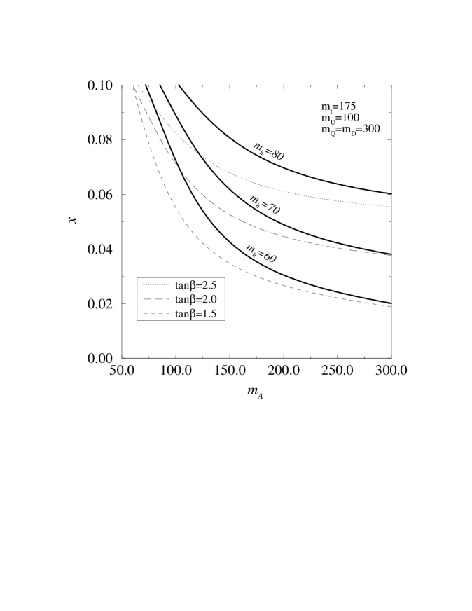
Figure 3: The effect of the CP-even and CP-odd Higgs masses $m_{h}$ and $m_{A}$ on $x$ ($x$ is defined in eq. (2.2)). All the numbers are in GeV. The mixing parameters have been set to zero. With the thin lines, we show as an alternative parametrization the value of $x$ as a function of $\tan\!\beta$ (at $\bar{\mu}=200$ GeV) in the present scheme.

In Fig. 3 the value of $x$ is shown as a function of $m_{A}$ for the reference set of parameters with three values of $\tan\!\beta$ (thin lines) and three values of the lightest Higgs mass $m_{h}$ (thick lines). We recall from eq. (2.2) that the requirement for a strong enough phase transition to sufficiently suppress the sphaleron rate in the broken phase is $x<0.03-0.04$. First, we notice that the best region for baryogenesis is a heavy CP-odd Higgs particle, as is already known [5]. Second, for the reference parameters, even the region $x<0.03$ can be reached with a sufficiently small Higgs mass (although then our results are less reliable, see Sec. 5 and below). This should be contrasted with the situation in the Standard Model where it appears that no Higgs mass is possible [19]. Hence the situation has definitely improved in the MSSM. However, the Higgs mass needed in the MSSM would be rather small, $m_{h}\raise 1.29167pt\hbox{$<$\kern-7.5pt\raise-4.73611pt\hbox{$\sim$}}70$ GeV. This might soon be excluded experimentally.

In Fig. 4 the effect of the top mass is shown, for fixed $\tan\!\beta$ (thin lines) and fixed $m_{h}=70$ GeV (thick lines). In contrast to the Standard Model (see Fig. 27 in [19]) a large top mass makes the situation more favourable for baryogenesis. The reason for the difference is that in the MSSM the top Yukawa coupling also appears in the dimensionally reduced 3d effective theory through squark interactions. The corrections induced for the scalar self-coupling are large and negative as seen in eqs. (4)–(4). However, since the corrections are large, they are also sensitive to the precise value of $h_{t3}$. A way to estimate the reliability of the results is their $\bar{\mu}$-dependence, which exists since $h_{t3}$ is fixed only at tree-level. By varying $\bar{\mu}$ from 200 Gev to 300 GeV for fixed $m_{h}$, the change in $x$ is less than 3% for $m_{t}\leq 175$ GeV. For $m_{t}=190$ GeV the change is about 10%. Hence the calculation becomes less reliable for large top mass.

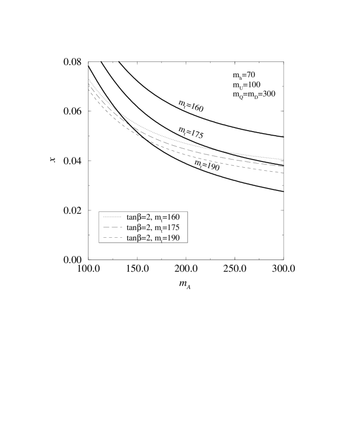
Figure 4: The effect of the top mass on $x$. Here the top mass is taken at tree-level, in accordance with the other uncertainties in the calculation. The thick lines are for constant $m_{h}=70$ GeV, the thin lines for constant $\tan\!\beta=2.0$. The mixing parameters have been set to zero.

It should be noted that we have kept $m_{Q}$ fixed when varying $m_{t}$. In fact, if $m_{t}$ is larger, then also $m_{Q}$ is likely to be larger, in order to keep the mass difference of left-handed stops and sbottoms small as required by phenomenological constraints [4, 5]. This effect would compensate for the increase in the strength of the transition with $m_{t}$ [7]. In principle, $m_{t}$ also directly affects the running of $m_{Q}^{2}(\bar{\mu}),m_{U}^{2}(\bar{\mu})$ to $\bar{\mu}=\bar{\mu}_{T}$, but these effects have been neglected here.

In Fig. 5 the effect of varying the squark mass parameter $m_{U}^{2}$ is shown, again separately for fixed $\tan\!\beta$ and for a fixed Higgs mass. A smaller $m_{U}$ makes the situation more favourable, as was already noted in [4, 5, 6]. In [6] even negative values for $m_{U}^{2}$ were considered. Here we cannot go to that region since then the squarks are not heavy any more and the effective theory is different, see Sec. 10. Nevertheless, one can see how the effect starts to arise. It is seen that for $m_{U}=50$ GeV even a Higgs mass in the region $m_{h}\sim 75$ GeV seems possible.

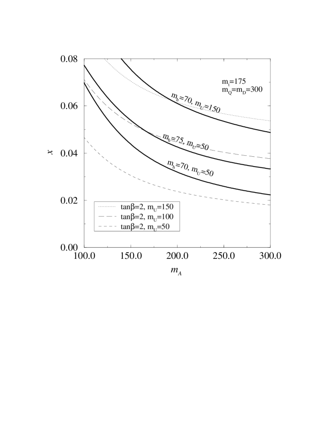
Figure 5: The effect of $m_{U}$ on $x$ for constant $m_{h}$ (thick lines) and $\tan\!\beta$ (thin lines). Note that at tree-level, the right-handed stop mass $m_{\tilde{t}_{R}}$ at zero temperature is given by $m_{\tilde{t}_{R}}^{2}=m_{U}^{2}+m_{t}^{2}$ for vanishing $\tilde{A}_{t}$ and $g^{\prime}$, see (8.6)–(8.8).

Finally, in Fig. 6 the effect of the mixing parameters is presented. Comparing with Fig. 3, one can see that $\mu$ has very little effect ($x$ is just slightly reduced at $m_{A}\sim 300$ GeV). Indeed, for large $m_{A}$ the mixing is determined exclusively by the combination $\tilde{A}_{t}$ appearing in the squark mass matrix. The effect of $\tilde{A}_{t}$ is that a large value makes $x$ larger. Phenomenologically, this is somewhat unfortunate [6] since one might wish to have a non-zero mixing in order to get smaller squark masses, which might help with the $R_{b}$-problem. The sbottom mixing parameter $\tilde{A}_{b}$ has practically no effect at all.

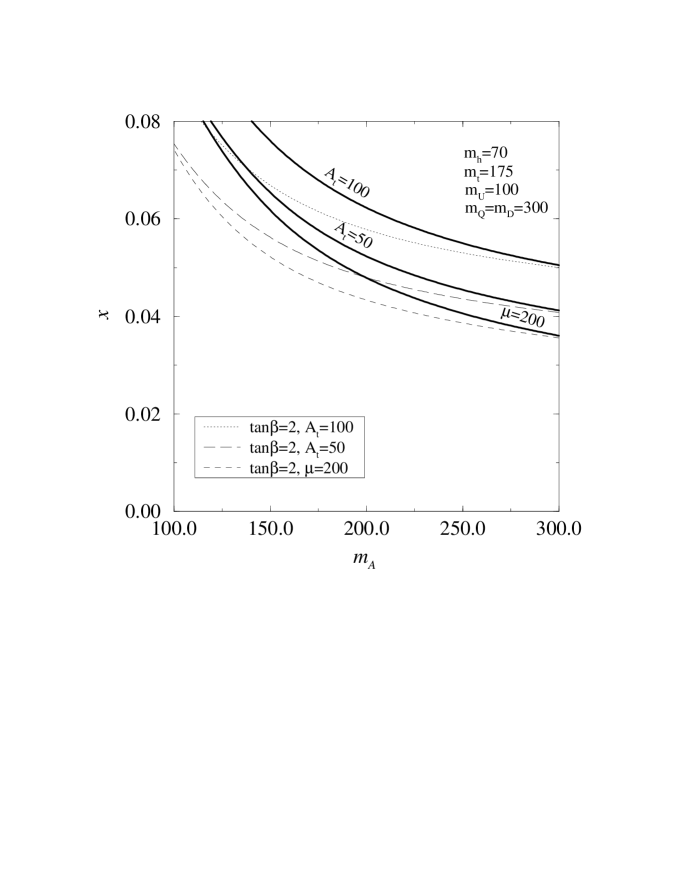
Figure 6: The effect of the mixing parameters on $x$ for constant $m_{h}$ (thick lines) and $\tan\!\beta$ (thin lines). The notation $A_{t}$ in the figure stands for $\tilde{A}_{t}$. If $\mu=0$ or if $m_{A}$ is large so that $\mu$ has little effect, the results are symmetric under $\tilde{A}_{t}\to-\tilde{A}_{t}$ so that only positive values are shown. For smaller $m_{A}$, the increase in $x$ is smallest when the signs of $\mu$ and $\tilde{A}_{t}$ are the same.

The overall conclusion is that for $m_{h}\raise 1.29167pt\hbox{$<$\kern-7.5pt\raise-4.73611pt\hbox{$\sim$}}m_{W}$ and small mixing, the transition might be strong enough for $m_{U}\raise 1.29167pt\hbox{$<$\kern-7.5pt\raise-4.73611pt\hbox{$\sim$}}50$ GeV and $m_{A}\raise 1.29167pt\hbox{$>$\kern-7.5pt\raise-4.73611pt\hbox{$\sim$}}200$ GeV. If the mixing is larger, one would need an even smaller $m_{U}$. These results agree to large extent with [4–7]. In any case, the situation has certainly improved with respect to the Standard Model.

10 The effective 3d theory in the case of light right-handed stops

It has been stressed in [6, 7] that small values of $m_{U}^{2}$ are phenomenologically allowed and are favourable for electroweak baryogenesis. On the other hand, it was pointed out in Sec. 5 that, if $m_{U}^{2}$ is small, one cannot integrate out the right-handed squarks and the relevant effective 3d theory is not the simple SU(2)+Higgs theory discussed in the previous Sections. In this Section we discuss in more detail at which point the 3d integration is no longer reliable and what the relevant 3d theory is then. We also indicate some non-perturbative effects which might arise beyond the perturbative ones discussed in [6, 7].

In [6], the case $m_{U3}\sim 0$ was investigated. From eq. (5.3) it is clear that then the integration does not work at all. To get a quantitative estimate of the $m_{U3}$ still allowed, one should compare 1-loop and 2-loop contributions to different parameters of the effective theory: $h_{t3}$-corrections first arise at 1-loop level and $g_{S3}$-corrections at 2-loop level, so that a comparison of tree-level and 1-loop results does not reveal much. The dominant 2-loop contributions were identified in [7].

The dominant 2-loop effect [7] is due to graphs of the type

$$V_{2l}=-2g_{S}^{2}{\cal D}_{\rm SSV}(m_{\tilde{t}_{R}},m_{\tilde{t}_{R}},0)$$ (10.1)

in the notation of [7, 23]. Here essentially $m^{2}_{\tilde{t}_{R}}=m_{U3}^{2}+h_{t}^{2}v_{2}^{2}/2$ (in [7] the coupling constant appearing in this formula is $h_{t}^{2}\sin^{2}\beta$ due to the limit $m_{A}\to\infty$). According to eq. (82) of [15], the term in (10.1) affects the dimensional reduction step of Sec. 4 only by changing the mass parameter $m_{2}^{2}$ by terms of the type

$$\delta m_{2}^{2}\sim\frac{T^{2}}{16\pi^{2}}g_{S}^{2}h_{t}^{2}\ln\frac{\bar{\mu}}{T}.$$ (10.2)

These terms are related to the running of $h_{t}^{2}(\bar{\mu})$ in the 1-loop thermal correction and hence their inclusion requires 1-loop renormalization of the top quark mass. In any case, these terms only affect the critical temperature and thus are not very important.

The (finite) 3d-part of the 2-loop contribution, on the other hand, is [15]

$$-2g_{S}^{2}{\cal D}^{\rm 3d}_{\rm SSV}(m_{\tilde{t}_{R}},m_{\tilde{t}_{R}},0)=8g_{S}^{2}m^{2}_{\tilde{t}_{R}}\frac{T^{2}}{16\pi^{2}}\biggl{(}\ln\frac{\bar{\mu}}{2m_{\tilde{t}_{R}}}+{\frac{3}{4}}\biggr{)}.$$ (10.3)

Now, if $m_{U3}$ is large enough and the transition is not too strong, this term can be expanded in powers of $h_{t}^{2}v_{2}^{2}/(2m_{U3}^{2})$. The first term, proportional to $v_{2}^{2}$, changes the mass parameter $m_{2}^{2}$ at 2-loop level, and is not very important. The second term is quartic in $v_{2}$ and changes the coupling $\lambda_{2}$ by

$$\delta\lambda_{2}^{2l}=-\frac{g_{S}^{2}h_{t}^{4}T^{3}}{8\pi^{2}m_{U3}^{2}}.$$ (10.4)

For clarity, we have here kept the coupling constants in their 4d normalizations so that powers of $T$ are written explicitly. The change in eq. (10.4) is negative, reducing the coupling constant $\lambda_{2}$ and consequently making baryogenesis more likely. Hence, as long as the expansion converges, this 2-loop correction works in a favourable direction also in the framework of the effective SU(2)+Higgs theory discussed in Secs. 5–7. However, when the effect becomes stronger, the convergence becomes worse and the higher order operators generated become important. The right-handed stops can no longer be integrated out but act as light degrees of freedom.

The expansion parameter of $U$-field integration can be estimated by comparing the 2-loop term in eq. (10.4) with the corresponding 1-loop term in eq. (5.21):

$$\delta\lambda_{2}^{1l}=-\frac{3}{16\pi}\frac{h_{t}^{4}T^{2}}{m_{U3}}.$$ (10.5)

Hence the expansion parameter is roughly

$$\frac{\delta\lambda_{2}^{2l}}{\delta\lambda_{2}^{1l}}={\frac{2}{3}}\frac{g_{S}^{2}T}{\pi m_{U3}}.$$ (10.6)

Consequently, to get convergence one needs $m_{U3}\raise 1.29167pt\hbox{$>$\kern-7.5pt\raise-4.73611pt\hbox{$\sim$}}T$.

What would be the effective theory if $m_{U3}\raise 1.29167pt\hbox{$<$\kern-7.5pt\raise-4.73611pt\hbox{$\sim$}}T$ and the integration does not converge? Let us assume that $m_{A}\to\infty$, the squark mixing parameters are small and $m_{Q}$ is relatively large as required by phenomenological constraints for a realistic top mass. Then all the other squark degrees of freedom apart from $U$ can be integrated out in the dimensionally reduced 3d theory. What remains can be written down immediately using 3d gauge invariance:

$$L = {\frac{1}{4}}F^{a}_{ij}F^{a}_{ij}+{\frac{1}{4}}G^{A}_{ij}G^{A}_{ij}$$ (10.7)

$$+ (D_{i}^{w}H)^{\dagger}(D_{i}^{w}H)+\tilde{m}_{H}^{2}H^{\dagger}H+\lambda_{H}(H^{\dagger}H)^{2}$$

$$+ (D_{i}^{s~{}}U)^{\dagger}(D_{i}^{s~{}}U)+\tilde{m}_{U}^{2}~{}U^{\dagger}U+\lambda_{U}~{}(U^{\dagger}U)^{2}$$

$$+ \gamma_{3}H^{\dagger}HU^{\dagger}U.$$

Here $D_{i}^{w}=\partial_{i}-ig_{3}\tau^{a}A_{i}^{a}/2$ and $D_{i}^{s}=\partial_{i}-ig_{S3}\lambda^{A}C_{i}^{A}/2$ (in this effective theory we have denoted the complex conjugate of the original $U$-field by $U$). At tree-level $\gamma_{3}=h_{t}^{2}\sin^{2}\!\beta\,T$, $\lambda_{U}=g_{S}^{2}T/6$ and $\tilde{m}_{U}^{2}=m_{U}^{2}+(4g_{S}^{2}/9+h_{t}^{2}/6+h_{t}^{2}\sin^{2}\!\beta\,/6)T^{2}$.

The steps needed for a more precise derivation of the theory in eq. (10.7) are in principle the following. First, make dimensional reduction as in Sec. 4 but in the theory where $m_{A}\to\infty$. In a precise study, it would be important to consistently include all the 1-loop corrections to the Yukawa couplings $h_{t}$ appearing in different places. Second, integrate out the heavy fields $Q,D,A_{0},C_{0}$ as in Sec. 5. Finally, make vacuum renormalization in order to fix the $\overline{\mbox{\rm MS}}$-parameters in terms of physical parameters. In particular, one should renormalize $m_{U}^{2}(\bar{\mu})$ and $h_{t}(\bar{\mu})$ in addition to the Higgs sector parameters by calculating the stop and top masses at 1-loop level. All these steps are straightforward and parallel the ones presented in Secs. 4–8.

Let us stress that perturbatively the theory in eq. (10.7) reproduces the 1- and 2-loop results making the dominant effects in [6, 7]. In fact, the 3d theory also contains a resummation of IR-safe higher-loop contributions, so that it is expected to be more precise than direct perturbative calculations in 4d. More important, eq. (10.7) contains all the IR-problems of the theory and could be used for 3d Monte Carlo simulations. No such simulations are available at the moment for the complete theory. However, one can try to use the knowledge obtained from simulations of the SU(2)+Higgs sector to get some insight into the properties of the complete theory. We make two guesses.

1. In the simulations of the 3d SU(2)+Higgs theory it was found that in the symmetric phase the relevant degrees of freedom are non-perturbative bound states [19, 20, 22, 34]. The mass of e.g. the scalar bound state may differ much from the perturbative value, let alone from the tree-level value. If $\tilde{m}_{U}^{2}$ is positive at $T_{c}$ so that the SU(3)-part of eq. (10.7) is in its symmetric phase, one might expect the same phenomenon to take place here, only the effects would be stronger than in the SU(2)-sector. This is important since the results of [6, 7] strongly depend on $\tilde{m}_{U}^{2}$ and assume a tree-level value for it. In particular, the non-perturbative mass might be significantly larger than the perturbative and tree-level masses, in which case the light degrees of freedom of the theory at the phase transition point might again be described by the 3d SU(2)+Higgs model. This time, however, the derivation of the effective theory would have to be non-perturbative.

2. The symmetric structure of eq. (10.7) opens other interesting possibilities. At the phase transition, $\tilde{m}_{H}^{2}$ is close to zero, and if $\tilde{m}_{U}^{2}$ is also rather close to zero as proposed in [6], one might end up in a situation where also the charged and coloured field $U$ acquires a non-vanishing expectation value at some point during the transition. This kind of a multi-stage transition might naturally alter the mechanism of baryogenesis. Requiring the absence of colour and charge breaking during the transition, some constraints on the parameters were given in [6, 35].

A precise investigation of the possibilities proposed will have to wait for a detailed perturbative derivation and a lattice investigation of the theory in eq. (10.7), as well as for experimental data on the values of the unknown parameters.

11 Conclusions

We have constructed super-renormalizable 3d effective field theories describing the thermodynamics of the electroweak phase transition in MSSM. The derivation of these theories is perturbative and free of IR problems. The effective theories can then be used for further perturbative investigations if IR problems are believed under control, or better still, for non-perturbative Monte Carlo studies.

It was found that in a part of the parameter space, it is possible to reduce the effective theory to a 3d SU(2)+Higgs theory for which there already exist lattice results. However, it generically appears that when the reduction can be done that far, the transition tends to get rather weak for realistic Higgs masses. Pushing the parameters into the region of a stronger transition (a smaller right-handed stop mass parameter $m_{U}^{2}$), the convergence of the 3d heavy scale integrations gets worse.

It hence seems that for a strongly first-order transition, the relevant effective 3d theory may be more complicated than SU(2)+Higgs. A particularly appealing possibility is a model containing an SU(2) scalar doublet and an SU(3) scalar triplet. If $m_{U}^{2}$ indeed turns out to be small, this effective theory should probably be studied in more detail. As far as the derivation of the theory is concerned, the most important pieces missing at the moment are the expressions for the parameters $h_{t}(\bar{\mu}_{T})$ and $m_{U}^{2}(\bar{\mu}_{T}^{\prime})$ in terms of zero-temperature physical parameters beyond tree-level. The calculations required are straightforward and parallel the calculations presented in the present paper.

Appendix Appendix  A

In this appendix we give the formulas used for vacuum renormalization in Sec. 8. More complete expressions can be found e.g. in [32, 28] (for compact approximation schemes and some 2-loop corrections, see e.g. [36] and references therein).

The calculation of the 1-loop self-energies is organized as follows. We first shift the fields to the classical broken minimum. Then the mass eigenstates are identified and the 1-loop graphs needed for $\langle h(k)h(-k)\rangle$, $\langle h_{A}(k)h_{A}(-k)\rangle$ and $\langle Z_{\mu}(k)Z_{\nu}(-k)\rangle$ are calculated. In particular, the tadpole graphs have to be included since we are not at the exact quantum minimum. According to the general strategy of this paper, only quarks and squarks of the third generation are included in the loops.

For fixed $\tan\!\beta$, the location of the classical broken minimum of eq. (3.3) is obtained from

$$v_{1}=\frac{2m_{Z}\cos\beta}{\tilde{g}},\quad v_{2}=\frac{2m_{Z}\sin\beta}{\tilde{g}}.$$ (A.1)

At the broken minimum, the mass eigenstates corresponding to the physical neutral Higgs fields $h,H,h_{A}$ are obtained from the fields in eq. (3.2) with the rotations

$$h^{1}_{0} = \cos\!\alpha\,h+\sin\!\alpha\,H,$$ (A.2)

$$h^{2}_{0} = -\sin\!\alpha\,h+\cos\!\alpha\,H,$$ (A.3)

$$h^{1}_{3} = \cos\!\beta\,h_{G_{0}}-\sin\!\beta\,h_{A},$$ (A.4)

$$h^{2}_{3} = \sin\!\beta\,h_{G_{0}}+\cos\!\beta\,h_{A}.$$ (A.5)

At tree-level the angle $\alpha$ here is given by

$$\sin\!2\alpha\,=-\sin\!2\beta\,\frac{m_{A}^{2}+m_{Z}^{2}}{m_{H}^{2}-m_{h}^{2}},\quad\cos\!2\alpha\,=\cos\!2\beta\,\frac{m_{A}^{2}-m_{Z}^{2}}{m_{H}^{2}-m_{h}^{2}}.$$ (A.6)

At 1-loop level we use the physical pole masses for $m_{A}^{2}$, $m_{Z}^{2}$, $m_{h}^{2}$, $m_{H}^{2}$ and the angle $\alpha$ is determined from the expression for $\cos\!2\alpha\,$. After the redefinitions (A.2)–(A.5), the graphs contributing to $\langle hh\rangle$, $\langle h_{A}h_{A}\rangle$ and $\langle Z_{\mu}Z_{\nu}\rangle$ can easily be identified.

The formulas arising are slightly complicated by the fact that the left- and right-handed squarks mix. For the mass eigenstates, we will use the notation $m_{U\pm}^{2}$, $m_{D\pm}^{2}$ defined by

$$m_{U\pm}^{2}={\frac{1}{2}}\Bigl{[}m_{U1}^{2}+m_{U2}^{2}\pm\sqrt{(m_{U1}^{2}-m_{U2}^{2})^{2}+4m_{U12}^{4}}\Bigr{]}$$ (A.7)

and correspondingly for $m_{D\pm}^{2}$, where $m_{U1}^{2},\ldots$ are in (8.7)–(8.10). We also denote

$$\delta_{U}=\frac{1}{m_{U+}^{2}-m_{U-}^{2}},\quad\delta_{D}=\frac{1}{m_{D+}^{2}-m_{D-}^{2}}.$$ (A.8)

Some standard integrals often appearing are denoted as follows. For $|m_{1}-m_{2}|<k<m_{1}+m_{2}$,

$$F_{H}(k;m_{1},m_{2}) \equiv 1-\frac{m_{1}^{2}-m_{2}^{2}}{k^{2}}\ln\frac{m_{1}}{m_{2}}+\frac{m_{1}^{2}+m_{2}^{2}}{m_{1}^{2}-m_{2}^{2}}\ln\frac{m_{1}}{m_{2}}$$

$$- \frac{2}{k^{2}}\sqrt{(m_{1}+m_{2})^{2}-k^{2}}\sqrt{k^{2}-(m_{1}-m_{2})^{2}}\arctan\frac{\sqrt{k^{2}-(m_{1}-m_{2})^{2}}}{\sqrt{(m_{1}+m_{2})^{2}-k^{2}}}.$$

Especially,

$$F_{H}(m_{1};m_{2},m_{2})=2-2\sqrt{4r^{2}-1}\arctan\frac{1}{\sqrt{4r^{2}-1}},$$ (A.10)

where $r=m_{2}/m_{1}$ and $r>1/2$. Outside the displayed kinematic region, an analytic continuation is needed, and from that we only use the real part in calculating the masses. The imaginary parts arising are small. We also define a function $F_{Z}$ arising in the calculation of the Z-boson self-energy:

$$F_{Z}(m_{1},m_{2})\!\! = \frac{1}{12m_{Z}^{2}}\biggl{\{}2m_{1}^{2}(m_{1}^{2}-m_{2}^{2}+m_{Z}^{2})\ln\frac{m_{1}}{m_{Z}}+2m_{2}^{2}(m_{2}^{2}-m_{1}^{2}+m_{Z}^{2})\ln\frac{m_{2}}{m_{Z}}$$ (A.11)

$$+ \Bigl{[}m_{Z}^{4}-2m_{Z}^{2}(m_{1}^{2}+m_{2}^{2})+(m_{1}^{2}-m_{2}^{2})^{2}\Bigr{]}\Bigl{[}1+\ln\frac{m_{Z}^{2}}{m_{1}m_{2}}-\frac{m_{1}^{2}+m_{2}^{2}}{m_{1}^{2}-m_{2}^{2}}\ln\frac{m_{1}}{m_{2}}$$

$$+ F_{H}(m_{Z};m_{1},m_{2})\Bigr{]}+{\frac{2}{3}}m_{Z}^{4}-3m_{Z}^{2}(m_{1}^{2}+m_{2}^{2})-(m_{1}^{2}-m_{2}^{2})^{2}\biggr{\}}.$$

The irreducible graphs needed are shown in Fig. 7 and the tadpole graphs in Fig. 8. We leave out the common factor $1/(16\pi^{2})$ in the formulas below.

Figure 7: The graphs contributing to (a) the pole mass $m_{Z}$ of the Z-boson and (b) the masses $m_{h},m_{H},m_{A}$ of the CP-even Higgs bosons and the CP-odd Higgs boson. In the internal lines, solid lines are quarks and dashed lines are squarks of the third generation. Examples of couplings appearing are also shown.

The contributions to $\left.\langle h(k)h(-k)\rangle\right|_{k^{2}=-m_{h}^{2}}$ from the graphs in Fig. 7.b are

$$({\rm qq}):\!\! \!\!-3h_{t}^{2}\sin^{2}\!\alpha\,\Bigl{[}(6m_{t}^{2}-m_{h}^{2})\ln\frac{\bar{\mu}^{2}}{m_{t}^{2}}+2m_{t}^{2}+(4m_{t}^{2}-m_{h}^{2})F_{H}(m_{h};m_{t},m_{t})\Bigr{]}$$ (A.12)

$$\!\!+\Bigl{\{}h_{t}\to h_{b},m_{t}\to m_{b},\sin^{2}\!\alpha\,\to\cos^{2}\!\alpha\,\Bigr{\}},$$

$$({\rm SS1}):\!\! \!\!3(u_{s}^{2}\sin^{2}\!\alpha\,+w_{s}^{2}\cos^{2}\!\alpha\,-u_{s}w_{s}\sin\!2\alpha\,)\biggl{\{}\ln\frac{\bar{\mu}^{2}}{m_{U-}m_{U+}}$$ (A.13)

$$\!\!+2\delta_{U}^{2}m_{U12}^{4}\Bigl{[}F_{H}(m_{h};m_{U-},m_{U-})+F_{H}(m_{h};m_{U+},m_{U+})\Bigr{]}$$

$$\!\!+\delta_{U}^{2}(m_{U1}^{2}-m_{U2}^{2})^{2}\Bigl{[}1+\delta_{U}(m_{U1}^{2}+m_{U2}^{2})\ln\frac{m_{U-}}{m_{U+}}+F_{H}(m_{h};m_{U-},m_{U+})\Bigr{]}\biggr{\}}$$

$$\!\!+\Bigl{\{}u_{s}\to d_{s},w_{s}\to e_{s},\sin^{2}\!\alpha\,\leftrightarrow\cos^{2}\!\alpha\,,\sin\!2\alpha\,\to-\sin\!2\alpha\,,U\to D\Bigr{\}},$$

$$({\rm SS2}):\!\! \!\!\frac{3}{16}\tilde{g}^{4}(v_{2}^{2}\sin^{2}\!\alpha\,+v_{1}^{2}\cos^{2}\!\alpha\,+v_{1}v_{2}\sin\!2\alpha\,)\ln\frac{\bar{\mu}^{2}}{m_{Z}^{2}}$$ (A.14)

$$\!\!+\frac{3}{16}\tilde{g}^{4}(v_{2}^{2}\sin^{2}\!\alpha\,+v_{1}^{2}\cos^{2}\!\alpha\,+v_{1}v_{2}\sin\!2\alpha\,)\delta_{U}^{2}\biggl{\{}(m_{U2}^{2}-m_{U-}^{2})^{2}\Bigl{[}\ln\frac{m_{Z}^{2}}{m_{U-}^{2}}$$

$$\!\!+F_{H}(m_{h};m_{U-},m_{U-})\Bigr{]}+(m_{U2}^{2}-m_{U+}^{2})^{2}\Bigl{[}\ln\frac{m_{Z}^{2}}{m_{U+}^{2}}+F_{H}(m_{h};m_{U+},m_{U+})\Bigr{]}$$

$$\!\!+2m_{U12}^{4}\Bigl{[}1+\ln\frac{m_{Z}^{2}}{m_{U-}m_{U+}}+\delta_{U}(m_{U1}^{2}+m_{U2}^{2})\ln\frac{m_{U-}}{m_{U+}}+F_{H}(m_{h};m_{U-},m_{U+})\Bigr{]}\biggr{\}}$$

$$\!\!+\Bigl{\{}U\to D\Bigr{\}},$$

$$({\rm SS3}):\!\! \!\!6h_{t}^{4}v_{2}^{2}\sin^{2}\!\alpha\,\biggl{\{}\ln\frac{\bar{\mu}^{2}}{m_{U-}m_{U+}}+{\frac{1}{2}}\Bigl{[}F_{H}(m_{h};m_{U-},m_{U-})+F_{H}(m_{h};m_{U+},m_{U+})\Bigr{]}\biggr{\}}$$ (A.15)

$$\!\!+\Bigl{\{}h_{t}\to h_{b},v_{2}^{2}\sin^{2}\!\alpha\,\to v_{1}^{2}\cos^{2}\!\alpha\,,U\to D\Bigr{\}},$$

$$({\rm SS4}):\!\! \!\!-{\frac{3}{2}}\tilde{g}^{2}h_{t}^{2}\Bigl{(}v_{2}^{2}\sin^{2}\!\alpha\,+{\frac{1}{2}}v_{1}v_{2}\sin\!2\alpha\,\Bigr{)}\ln\frac{\bar{\mu}^{2}}{m_{Z}^{2}}$$ (A.16)

$$\!\!-{\frac{3}{2}}\tilde{g}^{2}h_{t}^{2}\Bigl{(}v_{2}^{2}\sin^{2}\!\alpha\,+{\frac{1}{2}}v_{1}v_{2}\sin\!2\alpha\,\Bigr{)}\delta_{U}^{2}\biggl{\{}\Bigl{[}(m_{U2}^{2}-m_{U-}^{2})^{2}+m_{U12}^{4}\Bigr{]}\Bigl{[}\ln\frac{m_{Z}^{2}}{m_{U-}^{2}}$$

$$\!\!+F_{H}(m_{h};m_{U-},m_{U-})\Bigr{]}+\Bigl{[}(m_{U2}^{2}-m_{U+}^{2})^{2}+m_{U12}^{4}\Bigr{]}\Bigl{[}\ln\frac{m_{Z}^{2}}{m_{U+}^{2}}$$

$$\!\!+F_{H}(m_{h};m_{U+},m_{U+})\Bigr{]}\biggr{\}}+\Bigl{\{}h_{t}\to h_{b},v_{2}^{2}\sin^{2}\!\alpha\,\to v_{1}^{2}\cos^{2}\!\alpha\,,U\to D\Bigr{\}},$$

$$({\rm S1}):\!\! \!\!{\frac{3}{4}}\tilde{g}^{2}\cos\!2\alpha\,m_{U1}^{2}\biggl{(}\ln\frac{\bar{\mu}^{2}}{m_{Z}^{2}}+1\biggr{)}$$ (A.17)

$$\!\!-{\frac{3}{2}}\tilde{g}^{2}\cos\!2\alpha\,\delta_{U}\Bigl{[}(m_{U2}^{2}-m_{U-}^{2})m_{U-}^{2}\ln\frac{m_{U-}}{m_{Z}}-(m_{U2}^{2}-m_{U+}^{2})m_{U+}^{2}\ln\frac{m_{U+}}{m_{Z}}\Bigr{]}$$

$$\!\!-\Bigl{\{}U\to D\Bigr{\}},$$

$$({\rm S2}):\!\! \!\!3h_{t}^{2}\sin^{2}\!\alpha\,(m_{U1}^{2}+m_{U2}^{2})\biggl{(}\ln\frac{\bar{\mu}^{2}}{m_{Z}^{2}}+1\biggr{)}$$ (A.18)

$$\!\!-6h_{t}^{2}\sin^{2}\!\alpha\,\Bigl{(}m_{U-}^{2}\ln\frac{m_{U-}}{m_{Z}}+m_{U+}^{2}\ln\frac{m_{U+}}{m_{Z}}\Bigr{)}$$

$$\!\!+\Bigl{\{}h_{t}\to h_{b},\sin^{2}\!\alpha\,\to\cos^{2}\!\alpha\,,U\to D\Bigr{\}}.$$

The contributions to $\left.\langle h_{A}(k)h_{A}(-k)\rangle\right|_{k^{2}=-m_{A}^{2}}$ from the graphs in Fig. 7.b are

$$({\rm qq}):\!\! \!\!-3h_{t}^{2}\cos^{2}\!\beta\,\Bigl{[}(2m_{t}^{2}-m_{A}^{2})\ln\frac{\bar{\mu}^{2}}{m_{t}^{2}}+2m_{t}^{2}-m_{A}^{2}F_{H}(m_{A};m_{t},m_{t})\Bigr{]}$$ (A.19)

$$\!\!+\Bigl{\{}h_{t}\to h_{b},m_{t}\to m_{b},\cos^{2}\!\beta\,\to\sin^{2}\!\beta\,\Bigr{\}},$$

$$({\rm SS1}):\!\! \!\!3(u_{s}^{2}\cos^{2}\!\beta\,+w_{s}^{2}\sin^{2}\!\beta\,-u_{s}w_{s}\sin\!2\beta\,)\Bigl{[}\ln\frac{\bar{\mu}^{2}}{m_{U-}m_{U+}}$$ (A.20)

$$\!\!+1+\delta_{U}(m_{U1}^{2}+m_{U2}^{2})\ln\frac{m_{U-}}{m_{U+}}+F_{H}(m_{A};m_{U-},m_{U+})\Bigr{]}$$

$$\!\!+\Bigl{\{}u_{s}\to d_{s},w_{s}\to e_{s},\cos^{2}\!\beta\,\leftrightarrow\sin^{2}\!\beta\,,\sin\!2\beta\,\to-\sin\!2\beta\,,U\to D\Bigr{\}},$$

$$({\rm S1}):\!\! \!\!-{\frac{3}{4}}\tilde{g}^{2}\cos\!2\beta\,m_{U1}^{2}\biggl{(}\ln\frac{\bar{\mu}^{2}}{m_{Z}^{2}}+1\biggr{)}$$ (A.21)

$$\!\!+{\frac{3}{2}}\tilde{g}^{2}\cos\!2\beta\,\delta_{U}\Bigl{[}(m_{U2}^{2}-m_{U-}^{2})m_{U-}^{2}\ln\frac{m_{U-}}{m_{Z}}-(m_{U2}^{2}-m_{U+}^{2})m_{U+}^{2}\ln\frac{m_{U+}}{m_{Z}}\Bigr{]}$$

$$\!\!-\Bigl{\{}U\to D\Bigr{\}},$$

$$({\rm S2}):\!\! \!\!3h_{t}^{2}\cos^{2}\!\beta\,(m_{U1}^{2}+m_{U2}^{2})\biggl{(}\ln\frac{\bar{\mu}^{2}}{m_{Z}^{2}}+1\biggr{)}$$ (A.22)

$$\!\!-6h_{t}^{2}\cos^{2}\!\beta\,\Bigl{(}m_{U-}^{2}\ln\frac{m_{U-}}{m_{Z}}+m_{U+}^{2}\ln\frac{m_{U+}}{m_{Z}}\Bigr{)}$$

$$\!\!+\Bigl{\{}h_{t}\to h_{b},\cos^{2}\!\beta\,\to\sin^{2}\!\beta\,,U\to D\Bigr{\}}.$$

The contributions to the transverse part of $\left.\langle Z_{\mu}(k)Z_{\nu}(-k)\rangle\right|_{k^{2}=-m_{Z}^{2}}$ from the graphs in Fig. 7.a are

$$({\rm qq}):\!\! \!\!-{\frac{1}{2}}\tilde{g}^{2}\Bigl{[}(3m_{t}^{2}-m_{Z}^{2})\ln\frac{\bar{\mu}^{2}}{m_{t}^{2}}+{\frac{1}{3}}m_{Z}^{2}+(m_{t}^{2}-m_{Z}^{2})F_{H}(m_{Z};m_{t},m_{t})\Bigr{]}$$ (A.23)

$$\!\!+\Bigl{\{}m_{t}\to m_{b}\Bigr{\}},$$

$$({\rm SS}):\!\! \!\!-{\frac{1}{2}}\tilde{g}^{2}\Bigl{(}3m_{U1}^{2}-{\frac{1}{2}}m_{Z}^{2}\Bigr{)}\ln\frac{\bar{\mu}^{2}}{m_{Z}^{2}}$$ (A.24)

$$\!\!+3\tilde{g}^{2}\delta_{U}^{2}\Bigl{[}(m_{U2}^{2}-m_{U-}^{2})^{2}F_{Z}(m_{U-},m_{U-})+(m_{U2}^{2}-m_{U+}^{2})^{2}F_{Z}(m_{U+},m_{U+})$$

$$\!\!+2m_{U12}^{4}F_{Z}(m_{U-},m_{U+})\Bigr{]}+\Bigl{\{}U\to D\Bigr{\}},$$

$$({\rm S}):\!\! \!\!{\frac{3}{2}}\tilde{g}^{2}m_{U1}^{2}\biggl{(}\ln\frac{\bar{\mu}^{2}}{m_{Z}^{2}}+1\biggr{)}$$ (A.25)

$$\!\!-3\tilde{g}^{2}\delta_{U}\Bigl{[}(m_{U2}^{2}-m_{U-}^{2})m_{U-}^{2}\ln\frac{m_{U-}}{m_{Z}}-(m_{U2}^{2}-m_{U+}^{2})m_{U+}^{2}\ln\frac{m_{U+}}{m_{Z}}\Bigr{]}$$

$$\!\!+\Bigl{\{}U\to D\Bigr{\}}.$$

To the contributions in eqs. (A.12)–(A.25) one has to add the tadpole contributions from Fig. 8, since we are working around the classical minimum. The tadpole contributions to $\Pi_{h}(k^{2},\bar{\mu}),\Pi_{A}(k^{2},\bar{\mu}),\Pi_{Z}(k^{2},\bar{\mu})$ are

$$\Pi_{h}^{({\rm tad})} = -3\frac{\cos\!2\alpha\,}{\cos\!2\beta\,}\Pi_{A}^{({\rm tad})}$$

$$+ \frac{1}{2}\tilde{g}^{2}\biggl{[}\biggl{(}\frac{v_{1}\sin^{2}\!\alpha\,+v_{2}\sin\!2\alpha\,/2}{m_{H}^{2}}\biggr{)}v_{1}C_{h}+\biggl{(}\frac{v_{2}\cos^{2}\!\alpha\,+v_{1}\sin\!2\alpha\,/2}{m_{H}^{2}}\biggr{)}v_{2}S_{h}\biggr{]},$$

$$\Pi_{A}^{({\rm tad})} = -\frac{1}{4}\tilde{g}^{2}\cos\!2\beta\,\biggl{[}\biggl{(}\frac{v_{1}\cos^{2}\!\alpha\,+v_{2}\sin\!2\alpha\,/2}{m_{h}^{2}}+\frac{v_{1}\sin^{2}\!\alpha\,-v_{2}\sin\!2\alpha\,/2}{m_{H}^{2}}\biggr{)}v_{1}C_{h}$$ (A.27)

$$- \biggl{(}\frac{v_{2}\sin^{2}\!\alpha\,+v_{1}\sin\!2\alpha\,/2}{m_{h}^{2}}+\frac{v_{2}\cos^{2}\!\alpha\,-v_{1}\sin\!2\alpha\,/2}{m_{H}^{2}}\biggr{)}v_{2}S_{h}\biggr{]},$$

$$\Pi_{Z}^{({\rm tad})} = \frac{1}{2}\tilde{g}^{2}\biggl{[}\biggl{(}\frac{v_{1}\cos^{2}\!\alpha\,-v_{2}\sin\!2\alpha\,/2}{m_{h}^{2}}+\frac{v_{1}\sin^{2}\!\alpha\,+v_{2}\sin\!2\alpha\,/2}{m_{H}^{2}}\biggr{)}v_{1}C_{h}$$ (A.28)

$$+ \biggl{(}\frac{v_{2}\sin^{2}\!\alpha\,-v_{1}\sin\!2\alpha\,/2}{m_{h}^{2}}+\frac{v_{2}\cos^{2}\!\alpha\,+v_{1}\sin\!2\alpha\,/2}{m_{H}^{2}}\biggr{)}v_{2}S_{h}\biggr{]}.$$

Here

$$S_{h} = 3\Bigl{[}2h_{t}^{2}m_{t}^{2}-u_{s}^{2}-e_{s}^{2}+(d_{s}e_{s}-u_{s}w_{s})\cot\!\beta\,$$ (A.29)

$$- h_{t}^{2}({m_{U1}}^{2}+{m_{U2}}^{2})+\frac{1}{4}\tilde{g}^{2}({m_{U1}}^{2}-{m_{D1}}^{2})\Bigr{]}\biggl{(}\ln\frac{\bar{\mu}^{2}}{m_{Z}^{2}}+1\biggr{)}$$

$$- 12h_{t}^{2}m_{t}^{2}\ln\frac{m_{t}}{m_{Z}}+6h_{t}^{2}\Bigl{(}m_{U+}^{2}\ln\frac{m_{U+}}{m_{Z}}+m_{U-}^{2}\ln\frac{m_{U-}}{m_{Z}}\Bigr{)}$$

$$+ 6\delta_{U}u_{s}(u_{s}+w_{s}\cot\!\beta\,)\Bigl{(}m_{U+}^{2}\ln\frac{m_{U+}}{m_{Z}}-m_{U-}^{2}\ln\frac{m_{U-}}{m_{Z}}\Bigr{)}$$

$$+ 6\delta_{D}e_{s}(e_{s}-d_{s}\cot\!\beta\,)\Bigl{(}m_{D+}^{2}\ln\frac{m_{D+}}{m_{Z}}-m_{D-}^{2}\ln\frac{m_{D-}}{m_{Z}}\Bigr{)}$$

$$- {\frac{3}{2}}\tilde{g}^{2}\delta_{U}\Bigl{[}(m_{U2}^{2}-m_{U-}^{2})m_{U-}^{2}\ln\frac{m_{U-}}{m_{Z}}-(m_{U2}^{2}-m_{U+}^{2})m_{U+}^{2}\ln\frac{m_{U+}}{m_{Z}}\Bigr{]}$$

$$+ {\frac{3}{2}}\tilde{g}^{2}\delta_{D}\Bigl{[}(m_{D2}^{2}-m_{D-}^{2})m_{D-}^{2}\ln\frac{m_{D-}}{m_{Z}}-(m_{D2}^{2}-m_{D+}^{2})m_{D+}^{2}\ln\frac{m_{D+}}{m_{Z}}\Bigr{]},$$

$$C_{h} = \Bigl{\{}h_{t}\to h_{b},m_{t}\to m_{b},u_{s}\leftrightarrow d_{s},w_{s}\leftrightarrow-e_{s},\cot\!\beta\,\to\tan\!\beta\,,U\leftrightarrow D\Bigr{\}}.$$ (A.30)

Figure 8: The tadpole graphs needed in vacuum renormalization. The closed loops contain quarks and squarks of the third generation, and the single line may contain either of the CP-even Higgs particles. Representative coupling constants are shown.

The contributions to the heavier CP-even Higgs mass are obtained from the contributions to the lighter CP-even Higgs mass by changing $m_{h}^{2}\leftrightarrow m_{H}^{2}$, $\sin\!2\alpha\,\to-\sin\!2\alpha\,$, $\cos\!2\alpha\,\to-\cos\!2\alpha\,$, $\sin^{2}\!\alpha\,\leftrightarrow\cos^{2}\!\alpha\,$ inside the 1-loop formulas for $\Pi_{h}(-m_{h}^{2},\bar{\mu})$, as can be seen from eqs. (A.2), (A.3).

Erratum

(February, 1999)

In Appendix A, some loop contributions were erroneously omitted from the correlator $\left.\langle h(k)h(-k)\rangle\right|_{k^{2}=-m_{h}^{2}}$, Eqs. (A.12)-(A.18). These contributions, which do not have any scale dependence, are proportional to squark mixing parameters and are thus very small for the small mixings considered. Nevertheless, they should in principle be included.

In the notation of Fig. 7.b, the loops omitted are of the form

The results for these contributions, to be inserted between Eqs.(A.16),(A.17), are:

$$({\rm SS5}):\!\! \!\!-\frac{3}{\sqrt{2}}\tilde{g}^{2}(-u_{s}\sin\!\alpha+w_{s}\cos\!\alpha)(v_{1}\cos\!\alpha+v_{2}\sin\!\alpha)\delta_{U}m_{U12}^{2}\biggl{\{}\ln\frac{m_{U+}}{m_{U-}}$$

$$\!\!+\delta_{U}\Bigl{[}(m_{U2}^{2}-m_{U1}^{2})\Bigl{(}\delta_{U}(m_{U1}^{2}+m_{U2}^{2})\ln\frac{m_{U+}}{m_{U-}}-1\Bigr{)}$$

$$\!\!+(m_{U2}^{2}-m_{U-}^{2})F_{H}(m_{h};m_{U-},m_{U-})+(m_{U2}^{2}-m_{U+}^{2})F_{H}(m_{h};m_{U+},m_{U+})$$

$$\!\!+(m_{U1}^{2}-m_{U2}^{2})F_{H}(m_{h};m_{U-},m_{U+})\Bigr{]}\biggr{\}}$$

$$\!\!+\Bigl{\{}-u_{s}\sin\!\alpha+w_{s}\cos\!\alpha\to d_{s}\cos\!\alpha+e_{s}\sin\!\alpha,U\to D\Bigr{\}},\hskip 81.09035pt\mbox{(A.16.a)}$$

$$({\rm SS6}):\!\! \!\!12h_{t}m_{t}(-u_{s}\sin^{2}\!\alpha\,+{\frac{1}{2}}w_{s}\sin\!2\alpha\,)\delta_{U}m_{U12}^{2}$$

$$\!\!\times\Bigl{[}2\ln\frac{m_{U+}}{m_{U-}}+F_{H}(m_{h};m_{U-},m_{U-})-F_{H}(m_{h};m_{U+},m_{U+})\Bigr{]}$$

$$\!\!+\Bigl{\{}h_{t}\to h_{b},m_{t}\to m_{b},u_{s}\sin^{2}\!\alpha\,\to-d_{s}\cos^{2}\!\alpha\,,w_{s}\to e_{s},U\to D\Bigr{\}}.\hskip 25.60747pt\mbox{(A.16.b)}$$

Numerically, these graphs only affect Fig. 6 where non-vanishing mixing was considered. The curves for $\mu=200$ GeV do not change, since the omitted contributions are proportional to $\tilde{A}_{t},\tilde{A}_{b}$. The largest effect is for $\tilde{A}_{t}=100$ GeV: even then, the thin line (fixed $\tan\!\beta$) remains essentially unchanged. The thick line (fixed $m_{h}$), comes down by $\sim 0.005$. All the conclusions remain unchanged.

I thank M. Losada for bringing these omissions into my attention.

References

[1]
V.A. Kuzmin, V.A. Rubakov, and M.E. Shaposhnikov,
Phys. Lett. B 155 (1985) 36;
M.E. Shaposhnikov, Nucl. Phys. B 287 (1987) 757.
[2]
V.A. Rubakov and M.E. Shaposhnikov,
Usp. Fiz. Nauk 166 (1996) 493 [hep-ph/9603208].
[3]
S. Myint,
Phys. Lett. B 287 (1992) 325;
G.F. Giudice, Phys. Rev. D 45 (1992) 3177.
[4]
J.R. Espinosa, M. Quirós and F. Zwirner,
Phys. Lett. B 307 (1993) 106.
[5]
A. Brignole, J.R. Espinosa, M. Quirós and F. Zwirner,
Phys. Lett. B 324 (1994) 181.
[6]
M. Carena, M. Quirós and C.E.M. Wagner,
Phys. Lett. B 380 (1996) 81.
[7]
J.R. Espinosa, DESY 96-064 [hep-ph/9604320].
[8]
A.D. Linde,
Phys. Lett. B 96 (1980) 289;
D. Gross, R. Pisarski and L. Yaffe,
Rev. Mod. Phys. 53 (1981) 43.
[9]
P. Ginsparg,
Nucl. Phys. B 170 (1980) 388.
[10] T. Appelquist and R. Pisarski,
Phys. Rev. D 23 (1981) 2305.
[11] S. Nadkarni,
Phys. Rev. D 27 (1983) 917.
[12]
A. Jakovác, K. Kajantie and A. Patkós,
Phys. Rev. D 49 (1994) 6810;
A. Jakovác and A. Patkós,
Phys. Lett. B 334 (1994) 391; A. Patkós, P. Petreczky and J. Polonyi,
Ann. Phys. 247 (1996) 78;
A. Jakovác, A. Patkós and P. Petreczky,
Phys. Lett. B 367 (1996) 283.
[13]
A. Jakovác,
Phys. Rev. D 53 (1996) 4538.
[14]
K. Farakos, K. Kajantie, K. Rummukainen and M.
Shaposhnikov, Nucl. Phys. B 425 (1994) 67.
[15]
K. Kajantie, M. Laine, K. Rummukainen and
M. Shaposhnikov, Nucl. Phys. B 458 (1996) 90.
[16]
E. Braaten and A. Nieto,
Phys. Rev. D 51 (1995) 6990; 53 (1996) 3421.
[17]
G.D. Moore,
Phys. Rev. D 53 (1996) 5906.
[18]
K. Kajantie, K. Rummukainen and M. Shaposhnikov,
Nucl. Phys. B 407 (1993) 356;
K. Farakos, K. Kajantie, K. Rummukainen and M.
Shaposhnikov, Phys. Lett. B 336 (1994) 494;
Nucl. Phys. B 442 (1995) 317.
[19]
K. Kajantie, M. Laine, K. Rummukainen and M. Shaposhnikov,
Nucl. Phys. B 466 (1996) 189 [hep-lat/9510020].
[20]
E.-M. Ilgenfritz, J. Kripfganz, H. Perlt and A. Schiller,
Phys. Lett. B 356 (1995) 561; M. Gürtler, E.-M. Ilgenfritz,
J. Kripfganz, H. Perlt and A. Schiller,
hep-lat/9512022; hep-lat/9605042.
[21]
F. Karsch, T. Neuhaus and A. Patkós,
Nucl. Phys. B 441 (1995) 629;
F. Karsch, T. Neuhaus, A. Patkós and J. Rank,
Nucl. Phys. B 474 (1996) 217.
[22]
O. Philipsen, M. Teper and H. Wittig,
Nucl. Phys. B 469 (1996) 445.
[23]
P. Arnold and O. Espinosa,
Phys. Rev. D 47 (1993) 3546;
Phys. Rev. D 50 (1994) 6662 (E).
[24]
Z. Fodor and A. Hebecker,
Nucl. Phys. B 432 (1994) 127;
W. Buchmüller, Z. Fodor and A. Hebecker,
Nucl. Phys. B 447 (1995) 317.
[25]
J. Kripfganz, A. Laser and M.G. Schmidt,
Phys. Lett. B 351 (1995) 266.
[26]
J. Rosiek,
Phys. Rev. D 41 (1990) 3464; KA-TP-8-1995 [hep-ph/9511250] (E).
[27]
T. Appelquist and J. Carazzone,
Phys. Rev. D 11 (1975) 2856.
[28]
A. Donini,
Nucl. Phys. B 467 (1996) 3.
[29]
H.E. Haber and R. Hempfling,
Phys. Rev. D 48 (1993) 4280.
[30]
P. Arnold,
Phys. Rev. D 46 (1992) 2628.
[31]
P.H. Chankowski, A. Dabelstein, W. Hollik,
W.M. Mösle, S. Pokorski and J. Rosiek,
Nucl. Phys. B 417 (1994) 101.
[32]
P.H. Chankowski, S. Pokorski and J. Rosiek,
Phys. Lett. B 274 (1992) 191;
Nucl. Phys. B 423 (1994) 437;
A. Brignole,
Phys. Lett. B 281 (1992) 284;
A. Dabelstein, Nucl. Phys. B 456 (1995) 25;
V. Driesen, W. Hollik and J. Rosiek,
Z. Phys. C 71 (1996) 259.
[33]
K. Kajantie, M. Laine, K. Rummukainen and M. Shaposhnikov,
Phys. Rev. Lett., in press [hep-ph/9605288].
[34]
H.-G. Dosch, J. Kripfganz, A. Laser and M.G. Schmidt,
Phys. Lett. B 365 (1996) 213.
[35]
A. Kusenko, P. Langacker and G. Segre,
UPR-677-T [hep-ph/9602414].
[36]
J.A. Casas, J.R. Espinosa, M. Quirós and A. Riotto,
Nucl. Phys. B 436 (1995) 3; 439 (1995) 466 (E);
M. Carena, M. Quirós and C.E.M. Wagner,
Nucl. Phys. B 461 (1996) 407.
[37]
D. Delepine, J.-M. Gérard, R. Gonzalez Felipe and
J. Weyers, UCL-IPT-96-05 [hep-ph/9604440].
[38]
J.M. Cline and K. Kainulainen,
CERN-TH/96-76 [hep-ph/9605235].
[39]
M. Losada, RU-96-25 [hep-ph/9605266].