Out of Equilibrium Dynamics of a Quench-induced Phase Transition and Topological Defect Formation
Abstract
We study the full out-of-thermal-equilibrium dynamics of a relativistic classical scalar field through a symmetry breaking phase transition. In these circumstances we determine the evolution of the ensemble averages of the correlation length and topological defect densities. This clarifies many aspects of the non-perturbative dynamics of fields in symmetry breaking phase transitions and allows us to comment on a quantitative basis on the canonical pictures for topological defect formation and evolution. We also compare these results to those obtained from the field evolution in the Hartree approximation or using the linearized theory. By doing so we conclude about the regimes of validity of these approximations.
PACS Numbers: 11.15.Tk,11.27.+d, 11.30.Qc
I Introduction
The formation of topological defects is a general consequence of symmetry breaking phase transitions in field theories with a topologically non-trivial vacuum manifold, both in the early Universe [1, 2], and in a number of materials in the laboratory [3, 4, 5, 6].
To date predictions of the number and distributions of defects formed in these circumstances has relied on very simplistic heuristic models where some qualitative aspects of the phase transition are invoked but where all dynamics is sacrificed [7]. These are at the basis of large scale simulations of defect networks subsequently used to generate the energy density perturbations responsible for the formation of structure in the Universe [8].
Recently, considerable effort has been devoted to the development of more realistic methods to follow the approximate evolution of relativistic field theories in out of equilibrium settings [9, 10, 11] and, in this context, to account for the number of defects formed [12] at a symmetry breaking transition.
In this paper we perform the first complete fully non-linear dynamical study of a relativistic classical theory out of thermal equilibrium in a symmetry breaking phase transition. We compute the time evolution of many quantities of interest, such as the correlation length and the defect densities as well as their dependence on the choice of initial conditions and on the presence of external dissipation.
We then compare these results to other approaches found recently in the literature. We will show by explicit computation of the time evolution for the zero densities of our field in well specified and illustrative circumstances that both the Hartree approximation and the linearized theory have different merits in approximating the full classical evolution. By virtue of this comparison we also learn, in a quantitave manner, when they fail and consequently about the regimes of their applicability.
The results of this paper raise many extremely interesting new questions concerning the non-perturbative dynamics of relativistic fields away from thermal equilibrium. Our present methods rely heavily on the usage of extensive computational facilities. Rather than openly trying to tackle some of these new issues the intention of the presentation below will be a more modest one, openly restricted in its character to that of reporting on the finds of a numerical experiment. A more analytical approach must be sought in order to complete our understanding, though, and it is our intention to expand on our attempts in forthcoming publications. Nevertheless, we believe the present results constitute considerable quantitave progress on the usual canonical qualitative pictures of defect formation and evolution.
This paper is organized as follows. In section II we describe the theoretical background for the field evolution. We discuss the field equations for the full classical evolution, in the presence of external dissipation, and our choice of initial conditions, which for consistency we choose to follow a classical Boltzmann distribution. We then describe two approximation schemes to the classical evolution, namely the Hartree approximation and the linearized theory. In the latter case we present the exact analytical evolution and Halperin’s formula for the zero densities of the scalar field in a Gaussian theory. We finish this section by briefly describing our numerical procedure for the full classical evolution and the computation of approximate statistical ensemble-averaged quantities.
In section III we present our results. We show the fully non-equilibrium evolution of the scalar field correlation length as well as its zero and defect densities. We show explicitly that the latter can be counted at a given sensible field coarse-graining scale, independently of the necessary ultra-violet cut-off of our implementation. We also discuss the dependence of these results on our choice of initial conditions. We then proceed to compare these zero densities to those obtained from the Hartree approximation and the linearized theory, and to draw conclusions about the regimes of their applicability. Finally we present the evolution of the defect densities per correlation volume and seek to relate our results to the qualitative canonical arguments for defect formation and long time evolution: the Kibble mechanism and scaling conjectures.
In section IV we summarize our most important results, present our conclusions and point to questions raised by the present work we intend to study in the near future.
II Theoretical Background
In what follows we will be concerned solely with the evolution of a classical relativistic field theory. The role of quantum fluctuations on the evolution of our field is therefore simply neglected. This is done in the spirit of Statistical Relativistic Field Theories, e.g., [13].
Our neglect of all quantum aspects should, however, constitute an excellent approximation to the complete field dynamics at energies close to the phase transition temperature. This is a non-trivial statement to quantify in general but that can be made precise by treating the presence of the non-linear term in the usual perturbative loop expansion. The fundamental difference between the thermal and the quantum loop perturbative series then arises from the fact that the quantum expansion is organized in terms of increasing powers of while the thermal one is proportional to powers of the temperature , made adimensional by explicitly appearing in ratios with the mass scales in the theory. In the regime in which the temperature to mass ratios are very large compared to , quantum fluctuations can be safely neglected relative to their thermal equivalent. Another manifestation of the quantum nature of a field theory is that the energy spectrum becomes discrete and consequently the thermal distribution follows a Bose-Einstein distribution instead of its classical Boltzmann form. Both classical and quantum distributions coincide approximately for frequencies such that , showing again that quantum manifestations should become fundamental in the ultraviolet of the theory and/or at low temperatures, as is well known. Both these regimes are relatively unimportant for the studies presented below and, given our choice of the initial field configurations, may be probed only under extreme conditions in the evolution or measurements performed over the deep ultraviolet sector of the theory. We will not be concerned with these regimes below and that, given the fundamental difficulties inherent to a full quantum approach relative to the opportunities offered by the classical theory, constitutes our best justification for neglecting quantum fluctuations. Although somewhat unsatisfactory we believe this is in itself justifiable in view of the extremely interesting possibilities it permits, especially in opening a window for probing non-perturbative aspects of the field evolution at the phase transition. In this section we will proceed to describe the details of our full classical evolution as well as the basis for two approximations, the Hartree self-consistent evolution and the linearized theory. We conclude this section by presenting the predictions from the exact results possible in Gaussian theories and discussing our numerical methods.
A The Classical Theory
In what follows we will adopt the simplest collisional model displaying topological defects, i.e., we will be dealing with a classical scalar field theory in dimensions. In one spatial dimension a Boltzmann distributed classical field is always finite and therefore does not require re-normalization [13]. This choice of spatial dimensionality also allows us to guarantee, from a technical point of view, that we will be able to evolve numerically a discretized dynamical system with enough resolution on all scales and generate a sufficiently large number of field realizations in order to be able to compute true statistical ensemble-averaged quantities. In one spatial dimension and in equilibrium the Mermin-Wagner theorem [14] states that there is no long range order. In this sense there is no phase transition as understood canonically in terms of Thermodynamic quantities. In an out-of equilibrium evolution such as ours, however, spontaneous symmetry breaking certainly occurs, in the sense that the field chooses locally in space to fall towards either of the energetically equivalent vacua. In what follows we will therefore continue to use the term symmetry breaking phase transition in this sense. In any case, equilibrium in our evolution, as will be clear by the end of this section, can only be strictly achieved at zero temperature, where the Mermin-Wagner theorem ceases to apply. Field Theories in higher spatial dimensions will be considered in forthcoming work [15].
In order to trigger the transition we set up initially a large number of field configurations out of a micro-canonical statistical ensemble and, at , destabilize the system by changing instantaneously the sign and magnitude of the mass.
The evolution equations for , will then be taken to be
| (1) |
where is the scalar self-coupling, and the classical mass. The dissipation coefficient is included as we wish to describe a system in the presence of additional degrees of freedom. This a necessary condition in order to justify the use of a micro-canonical thermal distribution of fields as our initial conditions. Accordingly, the form of the evolution equations can be exactly obtained if our system, the scalar field, is assumed to be in contact with a much larger one, a thermal bath of oscillators, linearly coupled to . The result is a Langevin system with a simple Markovian dissipation kernel, characterized only by the constant value of , and a noise term, where the two are related by the fluctuation-dissipation theorem [16]. At zero bath temperature the system reduces to Eq. (1).
It is convenient and physically clarifying to consider the rescaled system by redefining the time and space variables as well as the field amplitudes as in
| (2) |
to be
| (3) |
where
| (4) |
The new dissipation constant, , has a clear physical interpretation. It is the ratio of the wave-length , for the mean scalar field to the diffusion length, , of a free Brownian particle in contact with the thermal bath. Whenever this ratio is small the diffusion length is large compared to the particle’s wave length and the only collisional effects present involve the interaction of the scalar field with itself. In the converse limit the system is dominated by dissipative effects to the bath and the dynamics obeys essentially a diffusion equation where the second derivative in Eq. (3) is negligible relative to the first and as a consequence oscillations and self-interactions play a secondary role.
The ratio is therefore our fundamental dynamical parameter. All other information about the system is encoded in the initial field configurations. To specify these we assume that, for , the system will be described by a free-field equation, with possibly a different mass parameter, ,
| (5) |
in thermal equilibrium at a given temperature . Our goal is to compute ensemble averages of several quantities throughout the evolution. In order to achieve this we generate initially a large number of field configurations out of a Boltzmann distributed statistical ensemble. This is, off course, the classical micro-canonical equilibrium distribution. The probability density functional, , for the field and its canonical conjugate momentum will be given by
| (6) |
where is the free-field Hamiltonian
| (7) |
where is 1-dimensional volume of our system, which will be taken to be much larger than the mean correlation length of the initial field configuration .
Since this is a Gaussian distribution we need only specify the mean-value and variance for the field and its conjugate momentum in order to characterize it. We do this most simply in Fourier space, where we have
| (8) |
and
| (9) |
with the dispersion relation
| (10) |
The same statistical field configuration could have been obtained by driving a linear (i.e., free of self-interactions) field to thermal equilibrium in contact with a reservoir at temperature , using a Langevin evolution equation, [13].
In order to trigger the symmetry breaking transition we proceed, at , to instantaneously change , in sign and in magnitude, thus forcing the system to leave thermal equilibrium and to evolve in a non-linear way, according to Eq. (1). This is the simplest way of de-stabilising the system and has the advantage of analytical tractability in the simplest cases. Because of this property it has been extensively used in the literature [9, 12], where the instantaneous change of is often referred to as a quench. In terms of bulk thermodynamical quantities it corresponds to a sudden decrease in Pressure, or in the language of Finite Temperature Field Theory a decrease in the theory’s effective potential. It is not clear to us, however, if such a triggering mechanism has a natural implementation in the Laboratory ***It is clear that this is not the mechanism of destabilising the theory in a cosmological context. Pressure quenches were used to drive liquid 4He systems through a super-fluid phase transition [4] but are thought to be accompanied by other energy loss mechanisms..
In order to compute average quantities we then evolve numerically a large number of random field realizations out of the statistical ensemble Eq. (8-9), using Eq. (1) and compute, at given time-intervals, their mean values over this set.
Before we proceed to present our results we will briefly describe two approximate schemes to the evolution described above, the Hartree approximation and the linearized theory. In the next section we will compare the results obtained by these three different approaches.
B The Hartree Approximation
A widely used approximation scheme to the full approach described in the previous section is the so called Hartree self-consistent approximation [19]. Unlike the naive perturbative expansion it has the virtue of remaining stable throughout the symmetry breaking transition. It is also fully renormalizable in the quantum case [10, 11]. Because of these characteristics the Hartree approximation has received quite a lot of attention in the recent literature as a means of performing out-of equilibrium computations in various situations [10, 11].
As a drawback it describes a theory where all energy transfers must be made through the mean-field and, as a consequence, in situations when the field evolution involves important energy transfers among modes with , it behaves poorly. Our objective below will be to make the latter statement more precise.
The Hartree approximation results from making the Lagrangian quadratic, by replacing the quartic term by an expression involving the average value of the quadratic field only. More interestingly, it can be seen to arise as the first order in a systematic perturbative expansion, in the parameter of an symmetric theory, see, e.g., [11].
Once this form for the Lagrangian density is assumed the corresponding evolution equations are required to be self-consistent, in the sense that the zero separation two-point function computed at each step of the evolution is the same one present in the effective Lagrangian, for the corresponding time.
In practice this can be achieved by replacing the cubic term in the Euler-Lagrange equation by
| (11) |
With this substitution the approximate evolution equations now describe a Gaussian field with an effective time-dependent mass. This allows us to easily compute the time dependent two-point function ,
| (12) | |||||
| (13) |
where we chose to write in terms of the usual positive and negative frequency modes, and respectively, as
| (14) |
These, in turn, obey the field evolution equations,
| (15) |
The initial conditions Eq. (8) and (9), can also be written in terms of the positive and negative frequency modes and . We obtain
| (16) |
For the Hartree scheme to be complete we have to impose a consistency equation, namely that the mean-field taken in Eq. (15) be the same as the result obtained from two-point correlation function calculated from Eq. (14). This gives,
| (17) |
Equations (15) and (17) together with the initial conditions Eq. (16) constitute a well posed initial value problem that can be easily solved numerically, for a discretized set of momenta. Note that once we obtain the time-dependent correlation function we have at our disposal all the information about the system since the Hartree approximation implicitly assumes a Gaussian distribution of fields.
Eq. (15) shows that the Hartree approximation is clearly collisionless as it describes the interactions of an infinite set of modes with a mean field. As a result energy transfer processes among the modes proceed without any exchange of momentum, necessarily through the mean field. The collisionless character of the Hartree approximation constitutes its greatest weakness and will bring about substantial differences to the behavior observed by evolving the scalar field using Eq. (1), as we will illustrate in the next section.
C The Linear Approximation
More severely one can neglect the interactions altogether simply by removing the cubic term in the evolution from Eq. (1). This is necessarily an extremely crude approximation but has the merit of making it possible to predict, given an initial Gaussian field configuration, all the relevant quantities analytically. It can be also assumed [as it has been done frequently in the literature, see [12]] that for certain parameter ranges the relevant evolution occurs in the period soon after the field leaves equilibrium and starts descending towards the minimum of the new potential. During this stage the potential can, in fact, be approximated by an inverted squared well, but as we will see later the non-linear aspects of the evolution will in well defined circumstances be relevant for the mechanism of defect production, altering substantially their numbers.
Since the evolution is linear, the distribution of fields will remain Gaussian for all times and we need only determine the two-point correlation function in order to have a full description of the system. This can easily be done analytically, with the positive and negative frequency modes being given by
| (18) | |||||
| (19) | |||||
| (20) | |||||
| (21) |
with
where and . Note that, modulo the effect of the external dissipation that damps all modes, the evolution is divided in the usual way between exponential [growing for and decaying for ] and oscillatory [for ].
D Analytical Results for the Gaussian Theory - Counting Zeros and Defects
In the special case of the linearized evolution exact analytical predictions are possible, which constitute an excellent test on our methods. These results are based on a well known computation, first derived by Halperin [17]. Given the knowledge of the equal time two-point function and its spatial derivatives it allows us to calculate the average spatial density of zeros , in a Gaussian distribution of fields. In one dimension Halperin’s formula becomes,
| (23) |
where, by translational invariance,
| (24) |
One of the simplest application of this result is for the case of a Boltzmann distribution of free quadratic fields, which corresponds to our initial conditions. We then have that our two-point function is explicitly time independent and takes the form
| (25) |
on a discrete periodic lattice, with and obeying the dispersion relation, Eq. (10). When substituted in Eq. (23) this gives
| (26) |
It is clear that , given by Eq. (26), diverges. Introducing an upper momentum cutoff we have that this is of the form †††For spatial dimension , . For , ..
Eq. (23) can be easily extended to both the Hartree and the linear evolutions, since in both cases the field distributions remain Gaussian for all times. This fact allows us to obtain a time dependent zero density, which can be written explicitly in terms of the propagating modes as
| (27) |
As before the result clearly diverges. This can be seen from the explicit analytical result, in the linear case, or numerically for the Hartree approximation. This divergence is a consequence of the existence of a too large number of zeros in arbitrarily small scales, too large in fact for the sums in Eq. (27) to converge to a finite result. The number of zeros that correspond to defects is, however, clearly independent of the behavior of the field deep in the ultra-violet. In order to measure the correct number of defects present in a given field configuration with zero crossings on all scales we must therefore introduced a coarse-graining scale, which we will naturally chose to be of the order [usually slightly larger] than the size of a defect [18]. In one spatial dimension there is an exact domain wall solution with a well defined width, given by .
When evolving the full non-linear theory we will thus have to introduce two relevant scales. An upper momentum cutoff, , which is related to the number of modes chosen to generate the initial conditions, and a coarse-graining scale, of the order of , used for calculating the defect density. This density has then to be shown explicitly not depend on the upper momentum cut-off. Given this cut-off scale we will also measure the zero density and compare it to the analytical predictions both from the linear and Hartree approximations.
E The Numerical Evolution
In order to perform the non-linear out-of-equilibrium evolution we have used a 128-processor parallel computer. We took advantage of this architecture to evolve in each processor a different random realization of the initial Boltzmann distributed scalar field. For each one of these we took the initial ultraviolet cut-off to correspond to a wave number of about 1000 and our spatial lattice to have 10625 sites. A defect’s width was always resolved with more than 12 lattice points. All quantities of interest were then computed at given time intervals by averaging over the ensemble.
To perform the numerical evolution we used a Second Order Staggered Leapfrog method. The corresponding set of equations for the field and its conjugate momentum are
| (28) | |||||
| (29) | |||||
| (30) |
where and is the time step.
The initial conditions were generated in Fourier space using a Normal Distributed random number generator and then converted to real space using a Fast Fourier Transform algorithm. For each chosen time step we measured the average density of zeros of the field [ by looking at sign changes at consecutive lattice points], the average density of defects [by counting the number of zeros in the coarse-grained field ] and the correlation function. Using the correlation function we have calculated the correlation length which we defined as the point at which the value of the correlation function, normalized at zero spacing to be unity, goes below . This also enables us to define defect and zero densities per correlation length volume.
Several precautions should be taken in order to guarantee a good accuracy of the results. The spatial step should be small enough to resolve the defects and the time step should obey the Courant condition
where is the physical lattice spacing, in order for the method to converge safely.
III The Results
A Testing our methods and exact analytical results for the Gaussian Theory
The simplest test we can perform on our procedure is to measure the zero densities in our numerical evolution in the special case of and compare the results to the exact predictions of the linearized theory.
This involves several aspects of our numerical data. Firstly we want to test whether our randomly generated initial conditions reproduce faithfully an average field configuration out of Boltzmann distribution and, in the affirmative case, whether the numerical evolution in the simple case of the linear theory coincide with the exact analytical results derived in sections II C and II D.
In order to do the latter we must necessarily introduce an ultraviolet momentum cut-off, . We note, however, that Halperin’s formula is still applicable for a finite number of modes, the exact result being given by Eq. (27) with finite limits in the sum. Therefore, the unavoidable introduction of a cut-off should not be an obstacle to the numerical verification of the analytical predictions. Before comparing the zero density obtained from the numerical linear evolution to the exact result we must pay attention to one last technical complication. When converting a finite set of amplitudes in -space to -space using the Fast Fourier Transform algorithm we are actually loosing resolution, in the sense of field structure, in the smallest scales, which in turn can lead to an underestimate of the number of zeros. We explicitly observed this problem when transforming a generated field configuration with amplitudes in momentum space to a grid with the same number of points in configuration space. A simple way of overcoming this difficulty is to, for a chosen , generate an extra number of modes of higher momentum with zero amplitude and then transform this set to -space. This corresponds basically to an increase in the number of points in real space (and thus in the spatial resolution) while keeping a given momentum cut-off fixed. How much precision we actually need is then decided by increasing the number of extra modes with zero amplitude until the average zero density converges to the analytical result for the Boltzmann distribution, given by Eq. (27). We were careful to follow this procedure even when the comparison to the linear results was unnecessary, in the case of the full classical evolution.
Having done this, we obtained an excellent agreement between the initial conditions and their numerical evolution and the exact analytical result, with a very small standard deviation within our ensemble, represented by the error bars in figure 1.
This also reassured us that the number of samples used in our ensemble, 128 as mentioned above, is large enough for us to obtain a good approximation to the exact ensemble averaged quantities.
B Non-linear Field and Defect evolution
Having performed the tests of subsection III A, we are now ready to analyse the evolution of the field in the presence of the non-linear term. As mentioned before, the evolution results depend only on one dynamical parameter and on the initial conditions which are completely specified by the values of the temperature, , and the mass, . In what follows we will assume the re-scaled evolution of Eq. (3) and drop tildes.
An example of the zero and defect density evolution is shown in fig. 2. As expected the density of the latter is always smaller than that of the former and independent of the chosen momentum cut-off. We also observe that for reasonably dissipated systems the defect and zero densities coincide for large times. The zero densities observed in the coarse-grained Gaussian initial field should not be taken strictly as defects, off course, as they lack the stability only obtained at later times as the field truly settles down locally at either of the energetically equivalent vacua.
The qualitative evolution of the field, in the aftermath of a sudden quench, can be seen to follow in general terms two quite different stages. Firstly, immediately after the quench, the negative curvature of the potential near the origin gives rise to instabilities in the fields, in the sense that if one neglects the cubic term in the evolution, which is initially taken to be small [because , by construction] the modes with momentum will evolve according to the real exponential forms of Eq. (19-21). The corresponding exponential growth distorts the original field configuration since the amplitudes for the unstable modes grow much larger than their characteristic value, typical of the thermal initial conditions, while the remaining amplitudes stay approximately the same, but for damping if dissipation is present. This represents a considerable deviation from the Boltzmann distributed initial field. This characteristic unstable behavior suggests that it is a good working hypothesis to assume the field in this initial stage follow approximately the linearized evolution. We will check and confirm this conjecture in what follows.
The instabilities shut down when the cubic term, in Eq. (3), grows large enough to compensate for the negative sign of the mass. This is the beginning of the second stage of the evolution, often referred to in the literature as re-heating since the field during this period tends again to a new maximum entropy configuration. The evolution at this stage is completely non-linear and inaccessible through the usage of the usual perturbative loop expansion.
At the beginning of re-heating the fields are severely red-shifted relative to a thermal distribution and energy redistribution among the modes must occur. As a result, in the absence of strong dissipation, the amplitude of the short wave-length modes grows while that of the long wave-length modes decreases. These two types of behavior are now not just characteristic of modes with momentum and , respectively, since among the latter the amplitude has also grown differentially, approximately with the exponential of their characteristic frequency Eq. (19). As a result of this flow of energy to smaller wave-lengths the field configurations change to display much more structure on smaller scales including those in which topological defects can be produced. After the first burst of energy transfer to smaller scales the resulting field configurations involving large gradients in small scales are energetically unfavoured and the field quickly evolves back to suppress them partially. This results in a series of oscillations in typical quantities, such as the zero densities or the correlation length, fig. 3 and 8.
In the presence of external dissipation, for non-zero, the instabilities grow in an analogous way, soon after the quench, but the process of energy redistribution or re-heating can be quite different. The presence of external dissipation, as we discussed above, can be seen as resulting from the existence of effective channels, i.e., modes of other fields, which compete with those of the scalar field for the energy transfered from its largest wave-length modes. The value of then determines the relative importance of these two types of channels. This competition among scalar field and channels external to it turns out to be absolutely crucial for the form of the evolution of the zero and defect densities.
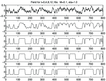
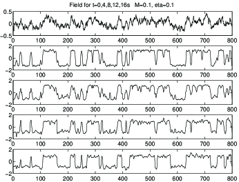
Schematically, with our choice of parameters, for , the system is always strongly dissipated and behaves much like a field without self-interactions [albeit stable] that freezes in very early. This can be clearly seen in the field profiles of fig. 5. The effective external channels therefore strongly dominate over the scalar field self- interactions and no signature of re-heating, such as the creation of zeros or a strong drop in correlation length, is observable.
For smaller values of the dissipation kernel , both self-interactions and dissipation are important, acting on the same kind of time scales. It is clear from our results that the transfer of amplitude among the modes occurs at well-defined stages of their oscillations. This is a subject of study in its own right, which is beginning to receive much attention in the context of the theory of re-heating after a period of inflationary expansion in the early Universe. Our objective in this paper is not to tackle this question but, in view of the strong analogies between the two problems, to merely point out that as a consequence of this behavior the creation of zeros and defects at re-heating proceeds by bursts. This is visible, e.g. in fig. 4.
When zeros and defects are created in these bursts the dissipation [ if not high enough ] and the field self-interactions are not sufficiently effective to suppress them immediately. As the momentary production shuts off, however, both these processes reduce the zero densities considerably. At the next burst another large amount of small scale structure can again be created but smaller than that at the previous instance. The field evolution then proceeds to dissipate it away and so on. As a result of these two competing processes the field oscillates between having quite large amounts of structure on small scales to having little, as both processes of creation and dissipation seem to be most efficient after the converse one has acted. These processes are clearly visible in the large oscillations undergone by the correlation length and defect densities. Profiles out of a field evolution in this dissipative regime is shown in fig. 6.
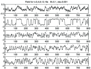
Finally, for small values of the dissipation coefficient, , the field is allowed to reach a favourable configuration before the dissipation has any sizable effect. The zero densities still oscillate in a similar fashion but field ordering in small scales now seems to be due to essentially the action of the field self-interactions. For this same reason the densities for large times are much larger that those obtained under the presence of larger dissipation. Its effect, if present at all, is only to damp all modes for large times. Modes on smaller scales are more strongly dissipated, though, due to the fact of possessing a larger natural frequency.
Snapshots of the field out of a characteristic evolution under the effect of very weak dissipation can be seen in the field profiles of 7.
Equivalently, the field evolution can be studied qualitatively by considering the time dependence of the correlation length. Fig. 8, shows the behavior of the correlation length in time under the effect of several values of the external dissipation.
It is clear that the correlation length increases in the first quasi-linear stage of the evolution, decreases at re-heating and increases again as the field organizes itself both via the effect of its self-interactions and due to the action of the external dissipation.
It is interesting to note, however, that the time evolution of the correlation length for large times, after re-heating, seems to display quantitatively different time trends depending on whether the self-organization proceeds by essentially the action of the scalar field self-interactions or results from the effect of the external dissipation. This seems to result in a linear time dependence in the first case and a well-known diffusive behavior with in the latter. This is illustrated in fig. 9, where it is also interesting to note that the slope of the linear correlation length growth for small dissipation is about of the speed of light.
This seems to suggest that the underlying field ordering proceeds by the free propagation of a well defined signal at a fraction of the speed of light as is often suggested in qualitative scenarios for domain formation and growth.
It is off course also possible that the linear behavior observed above will constitute merely a transient regime and that the evolution of the correlation length actually follows the same diffusive pattern, obtained under the effect of larger dissipation, but on a much larger time scale. For even smaller values of we observed the persistence of the linear behavior, but with smaller slopes, showing that the external dissipation is still playing a role in the field’s self-organization.
We also tried to determine the influence of our choice of initial conditions on the evolved defect densities. Initially, for an average Boltzmann field in the continuum limit, the spatial two-point correlation function has the exact form
| (31) |
This defines unambiguously the correlation length to be . Different choices of initial conditions corresponding to different masses therefore lead to quite distinct field configurations on given scales. Fig. 10 shows the defect density evolution for a choice of low dissipation, , and three different initial masses.
The initial temperature was chosen so as to guaranty that the field undergoes initial instabilities, i.e, so as to ensure the effectiveness of the quench as the mechanism driving the transition. The values chosen were such that , in our original Boltzmann distributed field. This results in small values of the temperature relative to the mass scales, of the order . It should be noted however, that the initial zero and defect densities are independent of this choice of temperature.
Given a choice of and the associated correlation length we expect, in rough terms, that the defect densities will be larger for smaller , as this is a qualitative indication of more structure on smaller scales. This can be clearly seen by comparing the initial magnitudes of the defect densities in figure 10, for three different choices of initial correlation lengths.
Fig. 10 shows a much more striking fact, however. It is clear that the number of defects produced at the phase transition is approximately independent of the initial densities even when these differ by over an order of magnitude. This is a clear indication of the importance of accounting correctly for the number of defects present at the time of re-heating and not sooner. This observed independence of the choice of initial defect densities is only characteristic of evolutions under the effect of small or null dissipation as in strongly dissipated systems re-heating is, as we have seen above, severely suppressed.
C Comparison with the results from the linearized theory and the Hartree approximation
In the previous section we presented and discussed the results for the full classical evolution of Eq. (3). In view of their extensive application to non-equilibrium problems in the literature it is extremely interesting to analyse how particular approximations to this classical theory perform relative to it.
In this subsection we briefly compare the results for the zero density evolution given by the full classical evolution to those obtained in the Hartree evolution and by considering the free field given by the linearized theory.
Fig. 11 and 12 show two examples of the zero density evolution computed in these three cases, and for relatively low and high dissipation, respectively. The observed difference between the zero densities given by the full classical evolution and those of the linear theory is quite simple to understand. For large , as we discussed above, the effective channels present implicitly in the form of the dissipation kernel, predominate over the scalar field self-interactions. As a result, under large dissipation, the observed evolution for the zero density is quite similar to that of a linear field, following approximately the results obtained by replacing, Eq. (19) and (21), into the expression for the zero density of a Gaussian theory Eq. (23). This procedure yields
| (32) |
Perhaps the most interesting feature of Eq. (32) is that it constitutes a lower bound on the defect density obtained from the classical theory, computed with the same initial field configuration at the same instant in time, for an evolution with any given . This fact remains interesting only for times that are not too large, since the field evolution under high dissipation quickly freezes in with a definite number of defects (see fig. 5), while Eq. (32) tends hopelessly to zero densities as time increases. This discrepancy for large times can be clearly seen in fig. 13.
In contrast to the previous situation, for evolutions under small external dissipation, the discrepancies between the zero density computed from the full classical theory and the linearized theory are quite dramatic at the time of re-heating. The re-heating process is accompanied by the production of a large number of zeros and defects that naturally go completely unaccounted for by the linear evolution. This is clearly visible in fig. 11.
The results obtained using the Hartree evolution also fail to reproduce those of the full classical evolution but in somewhat the opposite way. At re-heating the flow of energy from the infra-red to all other modes is very efficient in the Hartree evolution. When is small this indeed results in essentially the same number of created zeros as in the full evolution, as can be seen, e.g., in fig. 11. The collisionless character of the approximation, however, precludes the field from ridding itself of high gradient configurations on small scales. This results in the fundamental difference between the Hartree and the full evolution that, in the absence of dissipation, the number of zeros decreases in the latter but remains approximately constant after creation in the former. For short times, of the order of up to , the Hartree approximations therefore yields a number of zeros always larger than the full classical evolution. For larger times and for reasonably dissipated systems (), the fact that the Hartree approximation leads to field configurations with more power on small scales than the full evolution implies that it can be more efficiently dissipated. The end result is than after the dissipation makes its effect noticeable, the zero density resulting from the Hartree evolution is smaller than that of the full theory. For sufficiently large times such densities nevertheless tend to a constant value thus freezing in, as in the case of the full classical theory, unlike what happens in the case of the linear evolution.
For evolutions under stronger dissipation and for relatively short times, such as can be seen in fig. 12, the discrepancy between the Hartree and the full classical evolution can be quite spectacular and the linear result turns out to constitute a much better approximation. This is a clear concrete example in which the presence of a truncated set of interactions actually leads to a much worse prediction than what could be obtained much more simply from a trivial, exactly solvable linear approximation.
D Correlation Volume Defect Densities, Scaling and the Kibble Mechanism
The evolution of the defect densities and of the field’s correlation length are interesting on their own right. However, it is clear that they can constitute two different ways of probing the same qualitative structure. Defects are associated with sites of space where the field changes quickly between its two distinct energetically equivalent minima and constitute therefore regions where the field two-point correlation decreases. For this very reason defect densities tell us statistically how many areas of almost fully correlated field exist in a given volume, allowing us to probe their mean characteristic size. This is in turn clearly a measure of the correlation length.
The defect densities per correlation length volume constitute therefore very interesting quantities, that lie at the basis of fundamental conjectures for defect and domain formation and evolution such as the Kibble mechanism and Scaling conjectures.
In figs. 14 and 15 we plot these densities for two different sets of initial conditions, with small and large initial correlation length, respectively.
The Kibble mechanism invokes precisely the value of the field’s correlation length in order to predict the defect density produced at a symmetry breaking phase transition. The correlation length is clearly a qualitative measure of the size of the volume over which the field has only small amplitude fluctuations. Defects on the other hand correspond to field configurations that interpolate between the energetically indistinguishable minima and should therefore lie at the boundaries of average correlated patches. At distances larger than the correlation length the field will be in either one of these minima. The Kibble mechanism further assumes in what is usually designated the geodesic rule that between such uncorrelated regions the continuous field should take the shortest path over its vacuum manifold. This results in the simple but powerful prediction that between two correlation volumes, in one spatial dimension, there will be a defect or not with probability of 1/2. This is naturally the predicted value for the correlation volume defect density.
Observing fig. 14 and 15 it is quite striking to notice that regardless of the value of and of the particular choice of initial conditions, the defect densities obtained at re-heating and thereafter are of the order of the prediction given by the Kibble mechanism within a factor of about .
During the stage of re-heating it is still quite apparent that energy transfers between different scales are large and that arguments based on local energy minimization will be much blurred by large fluctuations [20]. Consequently it is more interesting to investigate the behavior of the defect densities for times sufficiently large that the system will already have found an energy balance among all scales. Fig. 16 shows the evolution of the defects densities per correlation volume, for two relatively close low values of the dissipation and , and a larger time range. It is clear that the correlation volume density of defects tends to a constant for large times. This is evidence for the scaling behavior of the domain wall network, i.e., for the fact that the number of defects per correlation volume remains constant in time, approximately once re-heating is complete.
This is an extremely powerful observation as it states that the statistical evolution of a domain wall network is characterized by one single length scale. According to this conjecture the domain wall network is self-similar after rescaling, when in the scaling regime, and its statistical features can be known at all times given the knowledge of the correlation length. Fig. 16 also shows clearly that, for the same value of dissipation but different initial conditions the correlation length defect densities for evolutions under small dissipation result in the same large time defect densities. This is evidence for the fact that the scaling densities are in these circumstances also independent of the initial conditions, at energies above the transition.
Moreover the value for the defect density in the scaling regime, for the smaller dissipation parameter in fig. 16, is very close to that predicted by the Kibble mechanism. In contrast, it is extremely interesting to notice that for a slightly larger value of , the scaling defect density is about lower. This seems to indicate that the presence of additional degrees of freedom that compete with those of the scalar field for its energy, necessarily leads to scalar field configurations with lower scaling defect densities.
For evolutions under stronger dissipation the scaling regime is of no particular interest, however, as it corresponds to the trivial situation in which the field is frozen in and both defect densities and correlation length become constant in time. Both these remarks may have interesting realizations as scenarios for defect formation in the early Universe.
IV Conclusions
We presented a detailed study of the non-equilibrium dynamics of a classical scalar field theory in a symmetry breaking phase transition. In doing so we were able to probe regimes of field evolution where perturbation theory breaks down and extract conclusions about the detailed correlation length and topological defect density evolution. We showed that after an instantaneous quench a field develops momentary instabilities responsible for the growth of its amplitude during which the evolution is approximately linear, and on a later stage when stability around the true minimum is found evolves, in a period of re-heating very similar to that of inflationary scenarios. During this later stage the evolution proceeds in a strongly non-linear fashion so as to redistribute energy among all scales. We showed the effect of external dissipation in the evolution and established evidence for the independence of defect densities per correlation length on the choice of initial conditions as well as their approach to a scaling regime for large times. In passing we confronted the predictions of the Kibble mechanism to our results and discussed the effect of the external dissipation on the asymptotic defect densities. We have also shown the comparison between the zero densities given by the full classical evolution and the predictions from the linearized theory and the Hartree approximations thus clarifying when these approximate schemes are valid.
Finally we believe that the present work raises many new important questions about the evolution of relativistic fields away from thermal equilibrium. We are presently investigating the effect of an expanding background on topological defect production and evolution, in higher spatial dimensions, and studying the details of the energy redistribution during the phase transition. Both these subjects have important cosmological applications to the role of topological defects as the seeding mechanism for the formation of structure in the Universe and the theory of re-heating after a period of inflationary expansion.
Acknowledgements
It is a great pleasure for us to thank Salman Habib, Wojciech Zurek and Marcelo Gleiser for extremely useful suggestions. We also thank Ed Copeland, Ray Rivers and Graham Vincent for discussions and Alisdair Gill for comments on the manuscript. NDA’s and LMAB’s research was supported by J.N.I.C.T.- Programa Praxis XXI, under contracts BD/2794/93-RM and BD/2243/92-RM, respectively. This work was supported in part by the European Commission under the Human Capital and Mobility programme, contract no. CHRX-CT94-0423. We thank The Fujitsu/Imperial College Centre for Parallel Computing for generous allocation of resources.
REFERENCES
- [1] T. W. B. Kibble, J. Phys. A 9, 1387 (1976)
- [2] For a comprehensive review see A. Vilenkin and E. P. S. Shellard, Cosmic Strings and other Topological Defects (Cambridge University Press, Cambridge, England, 1994).
- [3] W.H. Zurek, Los Alamos preprint LA–UR–95–2269, Phys. Rep., in press; Acta Physica Polonica B 24, 1301–1311 (1993).
- [4] P. C. Hendy, N. S. Lawson, R. A. M. Lee, P. V. E. McLintock and C. D. H. Williams, Nature 368, 315 (1994).
- [5] V.M.H. Ruutu et al., Imperial College Pre-print IMPERIAL/TP/95–96/17, accepted for publication in Nature.
- [6] I. Chuang, R. Durrer, N. Turok and B. Yurke, Science 251, 1336 (1991) ; M.J. Bowick, L. Chander, E. A. Schiff and A. M. Srivastava, Science 263, 943 (1994) 943.
- [7] T. Vachaspati and A. Vilenkin, Phys. Rev. D 31, 3052 (1985)
- [8] Ya. B. Zeldovich, Mon. Not. Astron. Soc. 192, 663 (1980); A. Vilenkin, Phys. Rev. Lett. 46, 1169 (1981); 46, 1496(E) (1981).
- [9] D. Boyanovsky, D.-S. Lee, A. Singh, Phys. Rev. D 48, 800 (1993)
- [10] D. Boyanovsky and H. J. de Vega, Phys. Rev. D 47, 2343 (1993); H. J. de Vega and R. Holman , Phys. Rev. D 49, 2769 (1994); D. Boyanovsky, H. J. de Vega, D.-S. Lee and A. Singh, Phys. Rev. D 51, 4419 (1995).
- [11] F. Cooper, S. Habib, Y. Kluger, E. Mottola, J. P. Paz and P. R. Anderson, Phys. Rev. D 50 2848 (1994).
- [12] A. J. Gill and R. J. Rivers, Phys. Rev. D 51,6949 (1995); G. Karra and R. J. Rivers, Imperial College preprint Imperial/TP/95-96/28 and hep-ph/9603413.
- [13] G. Parisi, Statistical Field Theory (Addison-Wesley Publishing Company, Inc. 1988)
- [14] N. D. Mermin and H. Wagner, Phys. Rev. Lett. 22, 1133 (1966)
- [15] N. D. Antunes, L. M. A. Bettencourt and A. Yates, in preparation.
- [16] S. Habib and H. E. Kandrup, Phys. Rev. D 46, 5303 (1992)
- [17] B. I. Halperin, Statistical Mechanics of Topological Defects, published in Physics of Defect, proceedings of Les Houches, Session XXXV 1980 NATO ASI, editors Balian, Kléman and Poirier (North-Holand Press, 1981), 816 (1981). For a more comprehensive derivation see F. Liu and G. F. Mazenko, Phys. D Rev. 46, 5963 (1992).
- [18] S. Habib in Proceedings of NEEDS’94, Los Alamos, (September 1994)
- [19] S. J. Chang, Phys. Rev. D 12. 1071 (1975)
- [20] L. M. A. Bettencourt, T. S. Evans and R. J. Rivers, Phys.Rev. D 53, 668, (1996).