UWThPh-1996-31

hep-ph/9605248

1 Schemes of neutrino mixing

The investigation of the problem of neutrino masses and mixing is the central theme of today’s neutrino physics. This problem is very important for elementary particle physics. There is a general belief that its investigation is a way to discover new physics. The problem of the masses of the neutrinos has also an exceptional importance for astrophysics. If the neutrino masses are in the eV region, it will allow to solve the problem (or part of the problem) of dark matter.

After many years of investigations, the problem of neutrino masses and mixing is still far from being solved. At present we have several indications in favour of nonzero neutrino masses and mixing angle. These indications come first of all from the solar neutrino experiments (Homestake [1], Kamiokande [2], GALLEX [3] and SAGE [4]). There are also indications in favour of neutrino mixing from some experiments on the detection of atmospheric neutrinos [5, 6, 7] and from the LSND experiment [8] in which beam-stop neutrinos were detected.

In the future with new experiments Super-Kamiokande [9], SNO [10], CHORUS [11], NOMAD [12], CHOOZ [13], ICARUS [14], MINOS [15], COSMOS [16] and many others we can expect a real progress in the investigation of the problem of neutrino masses, neutrino mixing and neutrino nature.

I will start with the formulation of the hypothesis of neutrino mixing. In accordance with all existing experimental data, the interaction of neutrinos with matter is described by the standard $CC$ and $NC$ Lagrangians

$$\mathcal{L}_{I}^{CC}=-\frac{g}{2\sqrt{2}}\,j_{\alpha}^{CC}\,W^{\alpha}+h.c$$ (1)

$$\mathcal{L}_{I}^{NC}=-\frac{g}{2\cos{\theta_{W}}}\,j_{\alpha}^{NC}\,Z^{\alpha}$$ (2)

Here

$$j_{\alpha}^{CC}=2\sum_{l=e,\mu,\tau}\bar{\nu}_{lL}\,\gamma_{\alpha}\,l_{L}+\ldots$$ (3)

$$j_{\alpha}^{NC}=\sum_{l=e,\mu,\tau}\bar{\nu}_{lL}\,\gamma_{\alpha}\,\nu_{lL}+\ldots$$ (4)

are the standard charged and neutral currents (we are interested here only in the lepton part of these currents). Let us notice that the $CC$ interaction $\mathcal{L}_{I}^{CC}$ determines the option of flavour neutrinos: muon neutrino is the particle that produce muon in the process $\nu_{\mu}+N\rightarrow\mu^{-}+X$, and so on. In the $CC$ and $NC$ interactions flavour neutrinos take part.

From LEP data on the measurement of the total invisible width of decay of $Z$ it follows that the number of flavour neutrinos $n_{\nu_{f}}$ is equal to three [17]:

$$n_{\nu_{f}}=2.987\pm 0.016$$ (5)

The hypothesis of neutrino mixing is the assumption that a flavour neutrino field $\nu_{lL}$ is a mixture of fields of neutrinos with definite mass

$$\nu_{lL}=\sum_{i}U_{li}\nu_{iL}\;,\qquad l=e,\mu,\tau$$ (6)

Here $\nu_{i}$ is the field of the neutrino with the mass $m_{i}$ and $U$ is a unitary mixing matrix.

How many massive light neutrinos exist in nature? Let us stress that LEP data do not give us information about the number of neutrinos $\nu_{i}$ with a small mass $m_{i}$. In fact, assuming that $m_{i}\ll m_{Z}$, for the total invisible decay width of the $Z$ in the case of neutrino mixing we have [18]

$$\Gamma_{Z}^{inv}=\sum_{l}\sum_{i,k}{|U_{li}|}^{2}\,{|U_{lk}|}^{2}\,\Gamma^{0}(Z\rightarrow\nu\bar{\nu})$$ (7)

where $\Gamma^{0}(Z\rightarrow\nu\bar{\nu})$ is the standard decay width of the $Z$ into a pair of massless neutrino and antineutrino. Due to the unitarity of the mixing matrix, independently on the number of light neutrinos we have

$$\Gamma_{Z}^{inv}=n_{\nu_{f}}\,\Gamma^{0}(Z\rightarrow\nu\bar{\nu})$$ (8)

The number of massive neutrinos in different schemes of neutrino mixing is different and is varied from three to six (see the reviews [19, 20]). If the neutrino mass term is a Dirac one

$$\mathcal{L}^{D}=-\sum_{l,l^{\prime}}\overline{\nu_{l^{\prime}R}}\,M^{D}_{l^{\prime}l}\,\nu_{lL}+\mbox{h.c.}$$ (9)

($M^{D}$ is a complex non-diagonal matrix), to three neutrino flavours correspond three massive neutrinos $\nu_{i}$ $(i=1,2,3)$ and the flavour fields $\nu_{lL}$ are connected with the massive fields $\nu_{iL}$ by the relation

$$\nu_{lL}=\sum_{i=1}^{3}U_{li}\,\nu_{iL}$$ (10)

Here $U$ is a unitary $3\times 3$ matrix and $\nu_{i}$ is the field of the neutrino with mass $m_{i}$. In the case of a Dirac mass term, the Lagrangian is invariant under the global gauge transformations

$$\nu_{l}\rightarrow e^{i\alpha}\,\nu_{l}\;,\qquad l\rightarrow e^{i\alpha}\,l$$ (11)

where $\alpha$ is an arbitrary constant. The invariance under this transformation means that the total lepton number

$$L=L_{e}+L_{\mu}+L_{\tau}$$ (12)

is conserved and that $\nu_{i}$ are Dirac neutrinos ($\nu_{i}$ and $\bar{\nu}_{i}$ have opposite values of $L$). Processes like neutrinoless double-beta decay are forbidden in this scheme.

Dirac neutrino masses can be generated by the standard Higgs mechanism together with the masses of all the other fundamental fermions. Of course, in this case we have no explanation of the fact that neutrinos are the lightest fermions in nature.

In the models beyond the Standard Model, like GUT models, the total lepton number $L$ is not conserved. The most general neutrino mass term that does not conserve $L$ is the so called Dirac and Majorana ($D+M$) mass term

$$\mathcal{L}^{D+M}=\mathcal{L}^{M}_{L}+\mathcal{L}^{D}+\mathcal{L}^{M}_{R}$$ (13)

Here

$$\mathcal{L}_{L}^{M}=-\frac{1}{2}\sum_{l,l^{\prime}}{\overline{(\nu_{l^{\prime}L})^{c}}}\,M^{L}_{l^{\prime}l}\,\nu_{lL}+\mbox{h.c.}$$ (14)

$$\mathcal{L}_{R}^{M}=-\frac{1}{2}\sum_{l,l^{\prime}}\bar{\nu}_{l^{\prime}R}\,M^{R}_{l^{\prime}l}\,{(\nu_{lR})}^{c}+\mbox{h.c.}$$ (15)

where ${(\nu_{lL})}^{c}=C\bar{\nu}^{T}_{lL}$ is the charge conjugated component, $M^{L}$ and $M^{R}$ are complex non-diagonal symmetrical $3\times 3$ matrices and $\mathcal{L}^{D}$ is given by the expression (9). The fields with definite masses $m_{i}$ are in this case six Majorana fields $\chi_{i}$. This corresponds to the fact that the left-handed as well as the right-handed components enter in the mass term and the lepton number $L$ is not conserved.

The flavour neutrino fields $\nu_{lL}$ are connected with $\chi_{i}$ by the relation

$$\nu_{lL}=\sum_{i=1}^{6}U_{li}\,\chi_{il}$$ (16)

where the fields $\chi_{i}$ satisfy the Majorana condition

$$\chi_{i}=\chi_{i}^{c}=C\bar{\chi}_{i}^{T}$$ (17)

The six Majorana fields $\chi_{i}$ are connected with the right-handed components $\nu_{lR}$ by the relation

$${(\nu_{lR})}^{c}=\sum^{6}_{i=1}U_{\bar{l}i}\chi_{iL}$$ (18)

The mixing matrix $U$ in Eqs.(16) and (18) is a $6\times 6$ unitary matrix.

In the framework of the $D+M$ mixing scheme there exist the very attractive see-saw mechanism [21] of neutrino mass generation that connects the smallness of the neutrino masses with the violation of the lepton number at the large (GUT?) scale.

In the simplest case of one generation, the $D+M$ mass term has the form

$$\mathcal{L}^{D+M}=-\frac{1}{2}\,m_{L}\,\overline{(\nu_{eL})^{c}}\,\nu_{eL}-m_{D}\bar{\nu}_{R}\nu_{L}-\frac{1}{2}\,m_{R}\,{\bar{\nu}_{eR}}\,(\nu_{eR})^{c}+\mbox{h.c.}$$ (19)

The masses of the two Majorana particles (eigenvalues of the mixing matrix) are given by

$$m_{1,2}=\frac{1}{2}\left|m_{R}+m_{L}\mp\sqrt{{(m_{R}-m_{L})}^{2}+4m^{2}_{D}}\right|$$ (20)

Let us assume that [21]

$$m_{L}\simeq 0\;,\qquad m_{D}\simeq m_{F}\;,\qquad m_{R}\simeq M_{GUT}\gg m_{F}$$ (21)

where $m_{F}$ is the mass of the charged lepton or up quark. This assumption means that the lepton number is violated (by the last term of Eq.(19)) at a scale that is much larger than the electroweak scale. In this case, for the Majorana masses we have

$$m_{1}\simeq\frac{m^{2}_{F}}{M_{GUT}}\;,\qquad m_{2}\simeq M_{GUT}$$ (22)

In the general case of three generations, in the spectrum of the masses of Majorana particles there are three light masses (masses of neutrinos)

$$m_{i}\simeq\frac{{(m_{F}^{i})}^{2}}{M_{i}}\;,\qquad i=1,2,3\;,$$ (23)

and three very heavy masses $M_{i}\simeq M_{GUT}$. From the see-saw formula (23) it follows (in agreement with experimental data) that the neutrino masses are much smaller than the masses of the other fundamental fermions.

If all the Majorana neutrino masses are small, due to Eqs.(16) and (18), transitions $\nu_{l}\rightarrow{\bar{\nu}_{l^{\prime}L}}$ are possible. Here $\bar{\nu}_{l^{\prime}L}$ is the state of a sterile neutrino (quantum of the right-handed field $\nu_{l^{\prime}R})$. The existence of such transitions would be a clear signature of new physics.

We will discuss now methods which allow to reveal the effects of neutrino masses and mixing. Some latest data will be also presented.

2 Tritium $\boldsymbol{\beta}$-spectrum

The investigation of high energy part of the $\beta$-spectra is the classical method of the measurement of the ”electron neutrino mass”. In most experiments the decay

$${{}^{3}}H\rightarrow{{}^{3}}He+e^{-}+\bar{\nu}_{e}$$ (24)

is investigated. This is a superallowed decay and the electron spectrum is determined by the phase space. The spectrum of the decay of the molecular tritium

$$T_{2}\rightarrow(T{}^{3}He)^{+}+e^{-}+\bar{\nu}_{e}$$ (25)

is given by

$$\frac{dN}{dT}=C\,p\,E\sum_{i}W_{i}\left(Q_{i}-T\right)\sqrt{\left(Q_{i}-T\right)^{2}-m^{2}_{\nu}}F(E)$$ (26)

Here $E=T+m_{e}$ and $p$ is the electron energy and momentum, $m_{\nu}$ is the neutrino mass, $W_{i}$ is the probability of the transition to the state $i$ of the molecule $(T{}^{3}He)^{+}$, $Q_{i}=Q_{0}-V_{i}$, $V_{i}$ is the excitation energy of the final molecule, $Q_{0}$ is the energy release in the decay of ${}^{3}H$. The results obtained in the latest experiments are presented in the Table 1.

Table 1: The upper bounds for electron neutrino mass obtained in the latest ${{}^{3}}H$ experiments.

Group	$m_{\nu}$ (eV)	$m^{2}_{\nu}$ (eV2)
Tokyo	$<13$	$-65\pm 85\pm 65$
Zurich	$<11$	$-24\pm 48\pm 61$
Los Alamos	$<9.3$	$-147\pm 68\pm 41$
Livermore	$<7$	$-130\pm 20\pm 15$
Mainz	$<7.2$	$-39\pm 34\pm 15$
Troitsk	$<4.35$	$-4.1\pm 10.9$

As it is seen from the Table 1, in modern tritium experiments no indications in favour of nonzero neutrino masses were obtained. However, some anomaly was found in these experiments: in all experiments the average value of $m^{2}_{\nu}$ is negative (see the last column of the Table 1). This means that, instead of the possible deficit of the events at the end of the spectrum (that would corresponds to a positive $m^{2}_{\nu}$), some excess of events is observed. This excess is clearly seen in the spectrum measured in the Troitsk experiment [22]. According to my knowledge, there is no understanding of the origin of this anomaly at the moment.

Another method to reveal the effects of neutrino masses is the search for neutrinoless double $\beta$-decay ($(\beta\beta)_{0\nu}$-decay) of some even-even nuclei.

3 Neutrinoless double $\boldsymbol{\beta}$-decay

The process

$$(A,Z)\rightarrow(A,Z+2)+e^{-}+e^{-}$$ (27)

is allowed only if neutrinos are massive Majorana particles. The Hamiltonian of the process is given by

$$H_{I}=\frac{G_{F}}{\sqrt{2}}\,2\left(\bar{e}_{L}\gamma_{\alpha}\nu_{eL}\right)j^{\alpha}+\mbox{h.c.}$$ (28)

where $j^{\alpha}$ is the hadron charged current and $\nu_{eL}$ is a mixed field. The ${(\beta\beta)}_{0\nu}$-decay is a process of the second order of the perturbation theory and neutrino mixing enters into the matrix element of the process through the propagator

$$\overset{\rule{0.5pt}{10.0pt}}{\vphantom{\nu^{T}_{eL}}\nu_{eL}}(x_{1})\hskip-23.99997pt\overline{\vphantom{\overset{|}{\vphantom{\nu^{T}_{eL}}\nu_{eL}}}\hskip 23.99997pt\hskip 6.60004pt\vphantom{\overset{|}{\nu^{T}_{eL}}}}\hskip-6.60004pt\overset{\rule{0.5pt}{10.0pt}}{\nu^{T}_{eL}}(x_{2}) = \sum_{i}U_{ei}^{2}\frac{1-{\gamma}_{5}}{2}\,\overset{\rule{0.5pt}{10.0pt}}{\vphantom{\bar{\chi}_{i}}\chi_{i}}(x_{1})\hskip-22.0pt\overline{\vphantom{\overset{|}{\vphantom{\bar{\chi}_{i}}\chi_{i}}}\hskip 22.0pt\hskip 5.0pt\vphantom{\overset{|}{\bar{\chi}_{i}}}}\hskip-5.0pt\overset{\rule{0.5pt}{10.0pt}}{\bar{\chi}_{i}}(x_{2})\,\frac{1-{\gamma}_{5}}{2}C$$ (29)

$$= -\left(\sum_{i}U^{2}_{ei}m_{i}\right)\frac{i}{{(2\pi)}^{4}}\int d^{4}p\,\frac{e^{-ip(x_{1}-x_{2})}}{p^{2}-m^{2}_{i}}\,\frac{1-\gamma_{5}}{2}\,C$$

where we have taken into account that for a Majorana field

$$\chi_{i}^{T}=-\bar{\chi}_{i}\,C$$ (30)

For small values of the neutrino masses we can neglect $m_{i}^{2}$ in the denominator of Eq.(29). Thus, the matrix element of $(\beta\beta)_{0\nu}$-decay is proportional to

$$\langle m\rangle=\sum_{i}U^{2}_{ei}\,m_{i}$$ (31)

The matrix element $U_{ei}$ is in general complex. This means that some cancellation of the contributions of different Majorana neutrinos to $\langle m\rangle$ is possible. To illustrate this statement, let us assume that $CP$ is conserved in the lepton sector. In this case, the mixing matrix satisfies the condition $U_{ei}=U_{ei}^{*}\eta_{i}$, where $\eta_{i}=\pm i$ is the $CP$ parity of the Majorana neutrino with mass $m_{i}$. In this case, for the quantity $\langle m\rangle$ we have [23]

$$\langle m\rangle=\sum_{i}|U_{ei}|^{2}\,m_{i}\,\eta_{i}$$ (32)

If the $CP$ parities of the different $\nu_{i}$ are different, there are cancellations in Eq.(32).

There are about 40 experiments on the search for neutrinoless double $\beta$-decay going on. No indication in favour of this process have been found so far. The most stringent limits were obtained in the experiments searching for $(\beta\beta)_{0\nu}$ decay of ${}^{76}Ge$ and ${}^{136}Xe$. In the experiment of the Heidelberg-Moscow collaboration the following lower bound for the time of life of ${}^{76}Ge$ was found [24]:

$$T^{0\nu}_{1/2}>5.1\times 10^{24}\,\mbox{y}$$ (33)

From this bound it follows that $|\langle m\rangle|<(0.7-2.3)$ eV. In two years this collaboration plans to reach the limit $T^{0\nu}_{1/2}\simeq{2\times{10^{25}}}$ y. The Heidelberg-Moscow collaboration obtained for the time of life of the allowed decay ${}^{76}Ge\rightarrow^{76}Se+e^{-}+e^{-}+\bar{\nu}_{e}+\bar{\nu}_{e}$ the following impressive result:

$$T^{2\nu}_{1/2}=(1.43\pm 0.03\pm 0.13)\times{10^{21}}\,\mbox{y}$$ (34)

For the time of life of the $(\beta\beta)_{0\nu}$-decay of ${}^{136}Xe$, the Caltech-Neuchatel-PSI collaboration [25] obtained the following lower bound:

$$T^{0\nu}_{1/2}>3.4\times{10^{23}}\,\mbox{y}$$ (35)

In the nearest future, with many new experiments now in preparation (NEMO [26] and others), the sensitivity for the quantity $\langle m\rangle$ is planned to be approximately one order of magnitude better than the present sensitivity [27].

I will turn now to the discussion of

4 Neutrino oscillations

Neutrino oscillations were first considered by B. Pontecorvo [28]. If there is neutrino mixing and the neutrino masses are small enough, the state of a flavour neutrino $\nu_{l}$ with momentum $\vec{p}$ is given by a coherent superposition of the states of massive neutrinos

$$\left|\nu_{l}\right\rangle=\sum_{i}\left|i\right\rangle U^{*}_{li}$$ (36)

here $\left|i\right\rangle$ is the state of a neutrino with negative helicity, momentum $p$ and energy $E_{i}=\sqrt{m_{i}^{2}+p^{2}}\simeq p+m_{i}^{2}/2p$. For the amplitude of the transition $\nu_{l}\rightarrow\nu_{l^{\prime}}$ during the time $t$, from Eq.(36) we have

$$A_{\nu_{l}\rightarrow\nu_{l^{\prime}}} = \sum_{i}\langle\nu_{l^{\prime}}|i\rangle e^{-iE_{i}t}\langle i|\nu_{l}\rangle=$$ (37)

$$= \sum_{i}U_{l^{\prime}i}\,e^{-iE_{i}t}\,U^{*}_{li}=$$

$$= e^{-iE_{1}t}\sum_{i}U_{l^{\prime}i}\,e^{-\frac{i\Delta m^{2}_{i1}}{2p}R}\,U^{*}_{li}$$

Here $\Delta m^{2}_{i1}=m^{2}_{i}-m^{2}_{1}$ and $R\simeq t$ is the distance between the neutrino source and detector. From this expression it is obvious that neutrino oscillations can take place if there is neutrino mixing ($U$ is not a diagonal matrix) and if at least one neutrino mass difference squared $\Delta m^{2}$ satisfies the inequality

$$\Delta m^{2}\gtrsim\frac{p}{R}$$ (38)

with $\Delta m^{2}$ in $\mbox{eV}^{2},R$ in $m$ and $p$ in MeV. From this inequality it follows that the sensitivity to $\Delta m^{2}$ of experiments with neutrinos from different facilities varies from $\sim\mbox{eV}^{2}$ (accelerators) to $\sim{10^{-11}}\mbox{eV}^{2}$ (the sun). Thus, as it was first stressed by B. Pontecorvo, neutrino oscillations is a very powerful tool for the investigation of the problem of neutrino masses and mixing.

Many experiments on the search for oscillations have been done with neutrinos from reactors and accelerators (see Ref.[29]). No indication in favour of neutrino oscillations were found in all experiments, except the Los Alamos experiment [8]. In this experiment neutrinos are produced in the decays (at rest) $\pi^{+}\rightarrow\mu^{+}\nu_{\mu}$, $\mu^{+}\rightarrow e^{+}\nu_{e}\bar{\nu_{\mu}}$. There are no $\bar{\nu_{e}}$’s in the initial beam (the estimated relative yield of $\bar{\nu}_{e}$ from background is $\simeq 4\times{10^{-4}}$ at $E\geq 36\,\mbox{MeV}$). In the LSND experiment 9 events $\bar{\nu}_{e}+p\rightarrow e^{+}+n$ ($n+p\rightarrow d+\gamma$) were observed with a neutrino energy in the interval $36\,\mbox{MeV}\leq E\leq 60\,\mbox{MeV}$. The expected background is $2.1\pm 0.9$ events. These data were interpreted [8] as an indication in favour of $\bar{\nu}_{\mu}\rightarrow\bar{\nu}_{e}$ oscillations.

The most stringent limits on the parameters that characterize $\nu_{\mu}\leftrightarrows\nu_{e}$ oscillations were obtained in the BNL E776 [30] and KARMEN [31] experiments.

We have considered [32] the mixing of three massive neutrino fields and we have assumed that neutrino masses satisfy hierarchy

$$m_{1}\ll m_{2}\ll m_{3}$$ (39)

with $\Delta m^{2}_{21}=m^{2}_{2}-m^{2}_{1}$, that is relevant for the suppression of solar $\nu_{e}$’s. In this case, for the probability of the transitions $\nu_{l}\rightarrow\nu_{l^{\prime}}$ ($l^{\prime}\neq l$) of terrestrial neutrinos we have

$$P_{\nu_{l}\rightarrow\nu_{l^{\prime}}}=\frac{1}{2}\,A_{\nu_{l};\nu_{l^{\prime}}}\left(1-\cos{\frac{\Delta m^{2}R}{2p}}\right)$$ (40)

where $\Delta m^{2}=m^{2}_{3}-m^{2}_{1}$ is the largest mass difference squared and the amplitude of oscillations is given by

$$A_{\nu_{l};\nu_{l^{\prime}}}=4\,|U_{l^{\prime}3}|^{2}\,|U_{l3}|^{2}$$ (41)

The probability of $\nu_{l}$ to survive is given by

$$P_{\nu_{l}\rightarrow\nu_{l}}=1-\sum_{l^{\prime}\neq l}P_{\nu_{l}\rightarrow\nu_{l^{\prime}}}=1-B_{\nu_{l};\nu_{l}}\left(1-\cos{\frac{\Delta m^{2}R}{2p}}\right)$$ (42)

where

$$B_{\nu_{l};\nu_{l}}=\sum_{l^{\prime}\neq l}A_{\nu_{l^{\prime}};\nu_{l}}=4\,|U_{l3}|^{2}\left(1-|U_{l3}|^{2}\right)$$ (43)

From this relation we find

$$|U_{l3}|^{2}=\frac{1}{2}\left(1\pm\sqrt{1-B_{\nu_{l};\nu_{l}}}\right)$$ (44)

At any fixed value of $\Delta m^{2}$, from exclusion plots obtained in reactor and accelerator disappearance experiments we have

$$B_{\nu_{l};\nu_{l}}\leq B^{0}_{\nu_{l};\nu_{l}}\qquad(l=e,\mu).$$ (45)

From Eqs.(44) and (45) it follows that

$$|U_{l3}|^{2}\leq a^{0}_{l}\qquad\mbox{or}\qquad|U_{l3}|^{2}\geq 1-a^{0}_{l}$$ (46)

where

$$a^{0}_{l}=\frac{1}{2}\left(1-\sqrt{1-B_{\nu_{l};\nu_{l}}^{0}}\right)$$ (47)

We have used the results of the Bugey [33], CDHS [34] and CCFR84 [35] experiments and we have considered the interval $10^{-1}\,\mathrm{eV}^{2}\leq\Delta m^{2}\leq 10^{3}\,\mathrm{eV}^{2}$. From these results it follows that the parameters $a^{0}_{e}$ and $a^{0}_{\mu}$ are small ($a^{0}_{e}\leq 2\times 10^{-2}$ in the whole region of $\Delta m^{2}$ and $a^{0}_{\mu}\leq 10^{-1}$ for $\Delta m^{2}\gtrsim 5\times 10^{-1}\,\mbox{eV}^{2}$).

From solar neutrino data it follows that the value of $|U_{e3}|^{2}$ cannot be large. In fact, for the case of a hierarchy of neutrino masses that we have assumed, the probability of the solar neutrinos to survive is given by [36]

$$P_{\nu_{e}\rightarrow\nu_{e}}=|U_{e3}|^{4}+\left(1-|U_{e3}|^{2}\right)^{2}P^{1,2}_{\nu_{e}\rightarrow\nu_{e}}$$ (48)

where $P^{1,2}_{\nu_{e}\rightarrow\nu_{e}}$ is the survival probability due to the coupling of $\nu_{e}$ with $\nu_{1}$ and $\nu_{2}$. If the parameter $|U_{e3}|^{2}$ satisfies the inequality $|U_{e3}|^{2}\geq 1-a^{0}_{e}$, from Bugey data it follows that $P_{\nu_{e}\rightarrow\nu_{e}}\geq 0.92$ for all solar neutrino energies. Such large value of the survival probability is not compatible with solar neutrino data. Thus, we have only two allowed regions of the values of $|U_{e3}|^{2}$ and $|U_{\mu 3}|^{2}$:

1. $|U_{e3}|^{2}\leq a^{0}_{e}\ll 1$ and $|U_{\mu 3}|^{2}\leq a^{0}_{\mu}\ll 1$;

2. $|U_{e3}|^{2}\leq a^{0}_{e}\ll 1$ and $1\geq|U_{\mu 3}|^{2}\geq 1-a^{0}_{\mu}$.

I will discuss now neutrino oscillation in these two regions. In the region I $\nu_{\mu}\leftrightarrows\nu_{e}$ oscillations are suppressed. In fact, from Eq.(42) we have

$$A_{\nu_{\mu};\nu_{e}}\leq 4\,a^{0}_{\mu}\,a^{0}_{e}$$ (49)

In the Fig.1 this limit is presented by the curve passing through circles. We have also plotted in Fig.1 the LSND allowed region (the shadowed region between two solid lines) and the exclusion plots obtained in the KARMEN [31] and BNL E776 [30] experiments.

Limits on the amplitude of $\nu_{\mu}\leftrightarrows\nu_{e}$ oscillations more stringent than those given by Eq.(49) can be obtained if the exclusion plot found in the FNAL E531 experiment [37] on the search for $\nu_{\mu}\leftrightarrows\nu_{\tau}$ oscillations is taken into account. In fact, in linear approximation in the small quantities $a^{0}_{e}$ and $a^{0}_{\mu}$ we have

$$A_{\nu_{\mu};\nu_{\tau}}\simeq 4\,|U_{\mu 3}|^{2}$$ (50)

Thus, for the amplitude of $\nu_{\mu}\leftrightarrows\nu_{e}$ oscillations we have the following upper bound:

$$A_{\nu_{\mu};\nu_{e}}\leq A^{0}_{\nu_{\mu};\nu_{\tau}}\,a^{0}_{e}$$ (51)

where $A_{\nu_{\mu};\nu_{\tau}}\leq A^{0}_{\nu_{\mu};\nu_{\tau}}$ and $A^{0}_{\nu_{\mu};\nu_{\tau}}$ can be obtained (at any fixed value of $\Delta m^{2}$) from the exclusion plot found in the FNAL E531 experiment. The upper bound (51) is presented in Fig.1 by the curve passing through triangles. As it is seen from Fig.1, the LSND-allowed region is not compatible with the data of all the other experiments on the search for neutrino oscillations (if there is a neutrino mass hierarchy and the parameters $|U_{e3}|$ and $|U_{\mu 3}|$ are both small).

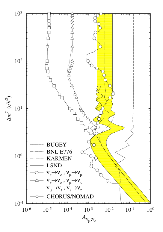
Figure 1: Exclusion regions in the $A_{\nu_{\mu};\nu_{e}}$–$\Delta m^{2}$ plane for small $\left|U_{e3}\right|^{2}$ and $\left|U_{\mu 3}\right|^{2}$.

In the linear approximation in $a^{0}_{e}$ and $a^{0}_{\mu}$, for the amplitude of $\nu_{e}\leftrightarrows\nu_{\tau}$ oscillations we have

$$A_{\nu_{e};\nu_{\tau}}\simeq 4\,|U_{e3}|^{2}$$ (52)

From the relations (42) and (52), it follows that, in the region of $\Delta m^{2}$ considered here, the amplitudes of $\nu_{\mu}\leftrightarrows\nu_{\tau}$ and $\nu_{e}\leftrightarrows\nu_{\tau}$ oscillations must be small:

$$A_{\nu_{\mu};\nu_{\tau}}\leq 4\,a^{0}_{\mu}$$ (53)

$$A_{\nu_{e};\nu_{\tau}}\leq 4\,a^{0}_{e}$$ (54)

There are no other constrains on the amplitudes $A_{\nu_{\mu};\nu_{\tau}}$ and $A_{\nu_{e};\nu_{\tau}}$ from the result of disappearance experiments. As it is well known, the search for $\nu_{\mu}\leftrightarrows\nu_{\tau}$ (and also $\nu_{e}\leftrightarrows\nu_{\tau}$) oscillations is going on in CERN (CHORUS [11] and NOMAD [12]). In the region of $\Delta m^{2}\geq 12\,\mbox{eV}^{2}$ these experiments will be sensitive to $A_{\nu_{\mu};\nu_{\tau}}\leq 2\times 10^{-4}$, which is much less than $4\,a^{0}_{\mu}$.

In the region II, due to unitarity of the mixing matrix,

$$|U_{e3}|^{2}\leq 1-|U_{\mu 3}|^{2}\leq a^{0}_{\mu}$$ (55)

Thus,

$$|U_{e3}|^{2}\leq 4\,\mbox{Min}(a^{0}_{e},a^{0}_{\mu})$$ (56)

For the amplitude of $\nu_{\mu}\leftrightarrows\nu_{e}$ oscillations, from the results of disappearance experiments we have the following upper bound

$$A_{\nu_{\mu};\nu_{e}}\leq 4\,|U_{e3}|\leq 4\,\mbox{Min}(a^{0}_{e},a^{0}_{\mu})$$ (57)

This bound (for $\Delta m^{2}>3\times 10^{-1}\,\mbox{eV}^{2}$) is less stringent than the bounds that were found in the KARMEN and BNL E776 experiments. For the amplitude of $\nu_{\mu}\leftrightarrows\nu_{\tau}$ oscillations, from the results of the disappearance experiments the same upper bound as in the case of region I can be obtained:

$$A_{\nu_{\mu};\nu_{\tau}}\leq 4|U_{\tau 3}|^{2}\leq 4a^{0}_{\mu}$$ (58)

If the parameters $|U_{e3}|^{2}$ and $|U_{\mu 3}|^{2}$ are in the region II, the oscillations $\nu_{e}\leftrightarrows\nu_{\tau}$ are strongly suppressed. In fact, from Eqs.(42), (55) and (56) we have

$$A_{\nu_{e};\nu_{\tau}}\leq 4\,\mbox{Min}(a^{0}_{e},a^{0}_{\mu})\ a^{0}_{\mu}$$ (59)

This bound is much stronger than the bound that was obtained in FNAL E531 experiment [37].

Thus, if the LSND result is confirmed by future experiments, the parameters $|U_{e3}|^{2}$ and $|U_{\mu 3}|^{2}$ cannot be both small (assuming that there is a hierarchy of neutrino masses), i.e. there is no hierarchy of couplings in the lepton sector. The only possible solution that is compatible with the LSND and all other neutrino oscillation experiments is the solution with small $|U_{e3}|^{2}$ and large $|U_{\mu 3}|^{2}$. This ”unnatural” neutrino mixing would mean that $\nu_{\mu}$ is the ”heaviest” neutrino.

5 Solar neutrinos

In conclusion we will consider briefly the solar neutrino problem. Probably at the moment the strongest indications in favour of neutrino mixing come from solar neutrino experiments. The reactions of the thermonuclear $p-p$ cycle, which are the main sources of solar $\nu_{e}$’s, are listed in the Table 2.

Table 2: Main sources of solar $\nu_{e}^{\prime}$s.

Reaction	Neutrino energies $E_{\nu}$ (MeV)	Expected fluxes ($\mbox{cm}^{-2}\mbox{sec}^{-1}$)
$p\,p\rightarrow d\,{e^{+}}\,\nu_{e}$	$\leq{0.42}$	$6.0\times{10^{10}}$
$e^{-}\,{{}^{7}Be}\rightarrow{{}^{7}Li}\,\nu_{e}$	0.86	$4.9\times{10^{9}}$
${}^{8}B\rightarrow{{}^{8}Be}\,e^{+}\,\nu_{e}$	$\leq{14}$	$5.7\times{10^{6}}$

In the last column of the Table 2 the fluxes calculated on the basis of the Standard Solar Model (SSM) [38] are presented. The fluxes of ${}^{8}B$ and other neutrinos depend strongly on the cross sections of nuclear reactions, on the temperature of the sun and other input parameters. There is, however, a general constraint on the solar neutrino fluxes. The solar energy is produced in the transition

$$2e^{-}+4p\rightarrow^{4}He+2\nu_{e}$$ (60)

Thus, the production of luminous energy of the sun is accompanied by the emission of neutrinos. If the sun is in a stable state, we have the following relation

$$\frac{1}{2}\,Q\sum_{i=pp,\ldots}\left(1-2\frac{\overline{E}_{i}}{Q}\right)\phi_{i}=L_{\odot}$$ (61)

Here $Q=4m_{p}+2m_{e}-m_{{}^{4}He}\simeq 26.7\,\mbox{MeV}$, $L_{\odot}$ is the luminosity of the sun, $R$ is the distance between the sun and the earth, $\phi_{i}$ is the total flux of neutrinos from the source $i$ ($i=pp,^{7}Be,\ldots$) and $\overline{E}_{i}$ is the average energy of the neutrinos from the source $i$. In the Table 3 the results of the four solar neutrino experiments (Homestake [1], Kamiokande [2], GALLEX [3] and SAGE [4]) are presented.

Table 3: Solar neutrino data.

Experiment	Counting rate (SNU)	Predicted rate (SNU)
Homestake
$(\nu_{e}{{}^{37}Cl}\rightarrow{{}^{37}Ar}e^{-})$	$2.56{}^{+0.17}_{-0.13}\pm 0.14$	$9.3\pm 1.4$
GALLEX
$(\nu_{e}{{}^{71}Ga}\rightarrow{{}^{71}Ge}e^{-})$	$77\pm{8.5}\pm{5}$	$131.5\pm{6}$
SAGE
$(\nu_{e}{{}^{71}Ga}\rightarrow{{}^{71}Ge}e^{-})$	$72{}^{+12}_{-10}{}^{+5}_{-7}$	$131.5\pm{6}$
KAMIOKANDE
$(\nu\,e\rightarrow\nu\,e)$	$\frac{\mathrm{data}}{\mathrm{SSM}}=0.51\pm{0.04}\pm{0.06}$

As it is seen from the Table 3, the observed event rates in all experiments are significantly less than the SSM expected rates. A few comments on this problem.

If we assume that $P_{\nu_{e}\rightarrow\nu_{e}}=1$, from the luminosity constraint (61) for the neutrino counting rate in the GALLEX and SAGE experiments we find the following lower bound:

$$Q_{Ga}=\sum_{i}\overline{\sigma}_{i}\,\Phi_{i}\geq\overline{\sigma}_{pp}\sum_{i}\Phi_{i}\simeq 80\,\mbox{SNU}$$ (62)

where $\overline{\sigma}_{i}$ is the average value of the cross section of the process $\nu_{e}+{{}^{71}Ga}\rightarrow e^{-}+{{}^{71}Ge}$. This lower bound does not contradict the rate measured in the GALLEX and SAGE experiments.

Let us consider the data of different solar neutrino experiments. We will assume only that $P_{\nu_{e}\rightarrow\nu_{e}}=1$. In the Kamiokande experiment, due to the high energy threshold of the detected electrons ($\simeq 7\,\mbox{MeV}$), only ${}^{8}B$ neutrinos are detected. From the data of this experiment, for the total flux of ${}^{8}B$ neutrinos it was obtained [39]

$$\Phi^{{}^{8}B}=(2.89\pm 0.21\pm 0.35)\times 10^{6}\,\mbox{cm}^{-2}\,\mbox{s}^{-1}$$ (63)

The main contribution to the event rate in the Homestake chlorine experiment comes from ${}^{8}B$ and ${}^{7}Be$ neutrinos. Using the value (63) of the ${}^{8}B$ flux for the contribution of the ${}^{7}Be$ neutrinos to the event rate of the chlorine experiment, we have the following upper bound:

$$Q_{Cl}(^{7}Be)\leq 0.46\,\mbox{SNU}$$ (64)

This upper bound is not compatible with the predictions of the existing Standard Solar Models:

$$Q_{Cl}^{\mathrm{SSM}}(^{7}Be)=1.1\pm 0.1\,\mbox{SNU}$$ (65)

The main contribution to the event rate of the gallium experiments comes from the $pp$, ${}^{7}Be$ and ${}^{8}B$ neutrinos. Using the luminosity constraint (61) and the value (63) of the ${}^{8}B$ neutrino flux, for the contribution of ${}^{7}Be$ neutrinos to the event rate in the GALLEX experiment we have the following upper bound:

$$Q_{Ga}(^{7}Be)\leq 19\,\mbox{SNU}$$ (66)

This value is significantly smaller than the values predicted by the existing Standard Solar Models:

$$Q_{Ga}^{\mathrm{SSM}}(^{7}Be)=34\pm 4\,\mbox{SNU}$$ (67)

Neutrino mixing is the most plausible explanation of the solar neutrino data. In fact, all the existing data can be explained if neutrino mixing enhanced by the MSW matter effects [40] is assumed. For the mixing parameters the following values were obtained (see Ref.[41])

$$\Delta m^{2}\simeq 5\times 10^{-6}\mbox{eV}^{2},\qquad\sin^{2}{2\theta}\simeq 8\times 10^{-3}$$ (68)

or (69)

$$\Delta m^{2}\simeq 5\times 10^{-5}\mbox{eV}^{2},\qquad\sin^{2}{2\theta}\simeq 0.8$$

These values were obtained under the assumption that solar neutrino fluxes are given by the BP [38] SSM model.

The solar neutrino experiments at the moment give us the most compelling indications in favour of neutrino mixing. However, new experimental data are needed to obtain an evidence for neutrino masses and mixing.

In conclusion, I will mention some model independent possibilities to obtain information about neutrino mixing from future solar neutrino experiments [42, 43]. In the Super-Kamiokande experiment, scheduled for 1996 [9] solar neutrinos will be detected through the observation (about 40 events/day) of the $ES$ process $\nu\,e\rightarrow\nu\,e$. In the SNO experiment, scheduled for 1997 [10], solar neutrinos will be detected through the observation of the $CC$ process $\nu_{e}\,d\rightarrow e^{-}\,p\,p$, the $NC$ process $\nu\,d\rightarrow\nu\,n\,p$ and also the $ES$ process $\nu\,e\rightarrow\nu\,e$. In both experiments, due to the high energy threshold, only ${}^{8}B$ neutrinos will be detected. The flux of initial ${}^{8}B$ neutrinos is given by

$$\Phi^{0}_{\nu_{e}}(E)=X(E)\,\Phi^{0}_{B}$$ (70)

where $\Phi^{0}_{B}$ is the unknown total flux and $X(E)$ is the known function of neutrino energy $E$ (determined mainly by the phase space factor of the decay ${{}^{8}B}\rightarrow{{}^{8}Be}\,e^{+}\,\nu_{e}$). The detection of solar neutrinos with the observation of the $CC$, $NC$ and $ES$ processes will allow to analyze the content of the beam of solar neutrinos on the earth, to determine the total flux $\Phi_{B}$ and the probability of solar neutrinos to survive $P_{\nu_{e}\rightarrow\nu_{e}}(E)$. In particular, it will be possible to check [43] in a model independent way if there are transitions of solar $\nu_{e}^{\prime}$s into sterile states. Indeed, the spectrum of the recoil electrons in the process $\nu\,e\rightarrow\nu\,e$ can be presented in the form

$$n^{ES}(T)=\int_{E_{\mathrm{min}}(T)}\left[\left(\frac{d\sigma}{dT}\right)_{\nu_{e}e}-\left(\frac{d\sigma}{dT}\right)_{\nu_{\mu}e}\right]\Phi_{\nu_{e}}(E)\,dE+\Sigma^{ES}(T)$$ (71)

where $T$ is electron kinetic energy, $(d\sigma/dT)_{\nu_{l}e}$ is the differential cross section of the process $\nu_{l}\,e\rightarrow\nu_{l}\,e$, $E_{\mathrm{min}}=T(1+\sqrt{1+2m_{e}/T})/2$, $\Phi_{\nu_{e}}(E)$ is the spectrum of $\nu_{e}$’s on the earth, that will be measured in the SNO experiment, and

$$\Sigma^{ES}(T) = \int_{E_{\mathrm{min}}(T)}\left(\frac{d\sigma}{dT}\right)_{\nu_{\mu}e}\sum_{l=e,\mu,\tau}P_{\nu_{l}\rightarrow\nu_{l}}\,X(E)\,dE\ \Phi_{B}$$ (72)

$$= \left\langle\sum_{l=e,\mu,\tau}P_{\nu_{l}\rightarrow\nu_{l}}\right\rangle_{T}X_{\nu_{\mu}e}(T)\,\Phi_{B}$$

where

$$X_{\nu_{\mu}e}(T)=\int_{E_{\mathrm{min}}(T)}\left(\frac{d\sigma}{dT}\right)_{\nu_{\mu}e}\,X(E)\,dE$$ (73)

is a known function of $T$. The function $\Sigma^{ES}(T)$ can be determined from experiment by the measurement of $n^{ES}(T)$ in the $ES$ process and $\Phi_{\nu_{e}}(E)$ in the $CC$ process. If the function $\Sigma^{ES}(T)/X_{\nu_{\mu}e}(T)$ depends on $T$, it means that the total probability of the transition of $\nu_{e}$’s into active states $\sum_{l=e,\mu,\tau}P_{\nu_{e}\rightarrow\nu_{l}}$ is less than one, i.e. that the solar $\nu_{e}$’s are transformed into sterile states.

There exist also the atmospheric neutrino anomaly observed by the Kamiokande [5], IMB [6] and Soudan 2 [7] experiments. This anomaly can be explained with $\nu_{\mu}\leftrightarrows\nu_{e}$ or $\nu_{\mu}\rightarrow\nu_{\tau}$ neutrino oscillations with $\sin^{2}2\theta\simeq 1$ and $\Delta m^{2}\simeq 10^{-2}\,\mbox{eV}^{2}$. Several long-baseline terrestrial neutrino experiments now in preparation will be sensitive to neutrino oscillations with $\Delta m^{2}\simeq(10^{-2}-10^{-3})\,\mbox{eV}^{2}$ and $\sin^{2}2\theta\gtrsim 0.1$ [15, 14, 44].

In conclusion, the problem of neutrino masses and mixing raised many years ago by B. Pontecorvo is the key problem of today’s neutrino physics. We have at the moment different indications in favour of non-zero neutrino masses and mixing angles. Future experiments could be decisive for this very important problem of physics and astrophysics.

I would like to express my gratitude to Carlo Giunti for fruitful collaboration and very useful discussions.

References

- [1] B.T. Cleveland et al., Nucl. Phys. B (Proc. Suppl.) 38, 47 (1995).
- [2] K. S. Hirata et al., Phys. Rev. D 44, 2241 (1991).
- [3] GALLEX Coll., Phys. Lett. B 357, 237 (1995).
- [4] V. Vermul, Talk presented at the International Workshop on Neutrino Telescopes, Venezia, February 1996.
- [5] Y. Fukuda et al., Phys. Lett. B 335, 237 (1994).
- [6] R. Becker-Szendy et al., Nucl. Phys. B (Proc. Suppl.) 38, 331 (1995).
- [7] M. Goodman, Nucl. Phys. B (Proc. Suppl.) 38, 337 (1995); J. Schneps, Talk presented at the International Workshop on Neutrino Telescopes, Venezia, February 1996.
- [8] C. Athanassopoulos et al., Phys. Rev. Lett. 75, 2650 (1995).
- [9] A. Suzuki, Talk presented at the International Workshop on Neutrino Telescopes, Venezia, February 1996.
- [10] A. Hime, Talk presented at the International Workshop on Neutrino Telescopes, Venezia, February 1996.
- [11] G. Rosa, Nucl. Phys. B (Proc.Suppl.) 40, 85 (1995); D. Macina, Talk presented at TAUP 95 Toledo (Spain), Sept. 1995.
- [12] A. Rubbia, Nucl. Phys. B (Proc.Suppl.) 40, 93 (1995); M. Laveder, Talk presented at TAUP 95 Toledo (Spain), Sept. 1995 (e-Print Archive: hep-ph/9601342).
- [13] R.I. Steinberg, Proc. of the International Workshop on Neutrino Telescopes, Venezia, March 1993.
- [14] ICARUS Coll., Gran Sasso Lab. preprint LNGS-94/99-I, May 1994.
- [15] MINOS Coll., NuMI note NUMI-L-63, February 1995; NUMI-L-79, April 1995.
- [16] N.W. Reay et al., Fermilab proposal P803, Oct. 1993.
- [17] Review of Particle Properties, Phys. Rev. D 50, 1173 (1994).
- [18] C. Jarlskog, Phys. Lett. B 241, 579 (1990); S.M. Bilenky, W. Grimus and H. Neufield, Phys. Lett. B 252, 119 (1990).
- [19] S.M. Bilenky and B. Pontecorvo, Phys. Rep. 41, 225 (1978).
- [20] S.M. Bilenky and S.T. Petcov, Rev. Mod. Phys. 59, 671 (1987).
- [21] M. Gell-Mann, P. Ramond, and R. Slansky, in Supergravity, ed. F. van Nieuwenhuizen and D. Freedman, (North Holland, Amsterdam, 1979) p. 315; T. Yanagida, Proc. of the Workshop on Unified Theory and the Baryon Number of the Universe, KEK, Japan, 1979; S. Weinberg, Phys. Rev. Lett. 43, 1566 (1979).
- [22] A.I. Belesev et al., Phys. Lett. B 350, 263 (1995).
- [23] M. Doi et al., Phys. Lett. B 102, 323 (1981); L. Wolfenstein, Phys. Lett. B 107, 77 (1981); S.M. Bilenky, N.P. Nedelcheva and S.T. Petcov, Nucl. Phys. B 247, 61 (1984); B. Kayser, Phys. Rev. D 30, 1023 (1984).
- [24] A. Balysh et al., Proc. of the Int. Conf. on High Energy Physics, Glasgow, August 1994.
- [25] J.C. Vuilleumier et al., Phys. Rev. D 48, 1009 (1993).
- [26] NEMO III. Proposal by the NEMO Coll., Laboratoire de l’Accelerateur Lineaire, LAL 94-29 (1994).
- [27] M. Moe and P. Vogel, Annu. Rev. Nucl. Part. Sci. 44, 247 (1994).
- [28] B. Pontecorvo, J. Exptl. Theoret. Phys. 33, 549 (1957) [Sov. Phys. JETP 6, 429 (1958)]; J. Exptl. Theoret. Phys. 34, 247 (1958) [Sov. Phys. JETP 7, 172 (1958)].
- [29] K. Winter, preprint CERN-PPE/95-165, Invited Talk at the 17th International Symposium on Lepton-Photon Interactions, Beijing, China, 1995.
- [30] L. Borodovsky et al., Phys. Rev. Lett. 68, 274 (1992).
- [31] B. Armbruster et al., Nucl. Phys. B (Proc. Suppl.) 38, 235 (1995).
- [32] S.M. Bilenky, A. Bottino, C. Giunti and C.W. Kim, preprint DFTT 2/96 (e-Print Archive: hep-ph/9602216).
- [33] B. Achkar et al., Nucl. Phys. B 434, 503 (1995).
- [34] F. Dydak et al., Phys. Lett. B 134, 281 (1984).
- [35] I.E. Stockdale et al., Phys. Rev. Lett. 52, 1384 (1984).
- [36] X. Shi and D.N. Schramm, Phys. Lett. B 283, 305 (1992).
- [37] N. Ushida Phys. Rev. Lett. 57, 2897 (1986).
- [38] J.N. Bahcall and R. Ulrich, Rev. Mod. Phys. 60, 297 (1988); J.N. Bahcall, Neutrino Physics and Astrophysics, Cambridge University Press, 1989; J.N. Bahcall and M.H. Pinsonneault, Rev. Mod. Phys. 64, 885 (1992); IASSNS-AST-95-24 (e-Print Archive: hep-ph/9505425).
- [39] J.N. Bahcall, Phys. Lett. B 338, 276 (1994).
- [40] S.P. Mikheyev and A.Yu. Smirnov, Yad. Fiz. 42, 1441 (1985) [Sov. J. Nucl. Phys. 42, 913 (1985)]; Il Nuovo Cimento C 9, 17 (1986); L. Wolfenstein, Phys. Rev. D 17, 2369 (1978); Phys. Rev. D 20, 2634 (1979).
- [41] GALLEX Coll., Phys. Lett. B 285, 390 (1992).
- [42] S.M. Bilenky and C. Giunti, Phys. Lett. B 311, 179 (1993); Nucl. Phys. (Proc. Suppl.) 35, 430 (1994).
- [43] S.M. Bilenky and C. Giunti, Phys. Lett. B 320, 323 (1994); Astropart. Phys. 2, 353 (1994); Z. Phys. C 68, 495 (1995).
- [44] K. Nishikawa, INS-Rep-924, April 1992; C.B. Bratton et al., Proposal to Participate in the Super-Kamiokande Project, Dec. 1992.