McGill/96-20

CERN-TH/96-76

hep-ph/9605235

May 6, 1996

Supersymmetric Electroweak Phase Transition:
Beyond Perturbation Theory

James M. Cline

McGill University, Montréal, Québec H3A 2T8, Canada,

and

Kimmo Kainulainen

CERN, CH-1211, Genève 23, Switzerland.

Abstract

We compute the three-dimensional effective action for the minimal supersymmetric standard model, which describes the light modes of the theory near the finite-temperature electroweak phase transition, keeping the one-loop corrections from the third generation quarks and squarks. Using the lattice results of Kajantie et al. for the phase transition in the same class of 3-D models, we find that the strength of the phase transition is sufficient for electroweak baryogenesis, in much broader regions of parameter space than have been indicated by purely perturbative analyses. In particular we find that, while small values of $\tan\beta$ are favored, positive results persist even for arbitrarily large values of $\tan\beta$ if the mass of the $A^{0}$ boson is between 40 and 120 GeV, a region of parameters which has not been previously identified as being favorable for electroweak baryogenesis.

1 Introduction

One of the fundamental questions in nature is the origin of the asymmetry of matter over antimatter in the universe. Although explanations abound, one of the most interesting possibilities is that the baryon asymmetry was created during the electroweak phase transition (EWPT) [1], using new physics at sufficiently low energies to be verifiable in anticipated experiments like LEP-II or the Large Hadron Collider. Although the EWPT is a first order transition in the standard model, it is too weakly so to fulfill Sakharov’s out-of-thermal-equilibrium requirement for generating baryons: any asymmetry created during the EWPT would be quickly erased afterwards by residual sphaleron interactions in the broken phase of the $SU(2)_{L}\times U(1)$ gauge theory [2]. Moreover it appears that the standard model has too little CP violation for electroweak baryogenesis [3].

It is therefore interesting to find out whether a more strongly first order EWPT is possible in extensions of the Standard Model, a prime example being its minimal supersymmetric extension, the MSSM, shown to be suitable for electroweak baryogenesis in ref. [4]. The phase transition has been studied in this model by means of the one-loop finite-temperature effective potential [5]-[8], with the result that there exist some regions of parameter space where electroweak baryogenesis is possible. However the perturbative approach should be viewed with skepticism because at finite temperature it becomes infrared divergent for small values of the Higgs field, which can be crucial for determining the critical temperature and Higgs field VEV at the phase transition.

To deal with the breakdown of perturbation theory, Kajantie et al. [2] have studied the EWPT of the Standard Model on the lattice. As they have emphasized however, almost any extension of the Standard Model can be reduced to an effective three-dimensional theory of one Higgs doublet interacting with $SU(2)$ gauge bosons, by integrating out all the modes with thermal masses larger than those of the longitudinal gauge bosons [9]. The beauty of this approach is that the effective theory need only be numerically studied once; after that it is simply a matter of matching the parameters of the fundamental theory onto this effective theory, which can be reliably done using perturbation theory.

In this paper we construct the effective 3-D Lagrangian corresponding to the MSSM at finite temperature, keeping the dominant effects proportional to the top quark Yukawa coupling. At the critical temperature it has the simple form

$$\bar{\cal L}_{3}=|(\partial_{i}-{\textstyle\frac{i}{2}}\bar{g}_{3}\vec{\tau}\cdot\vec{W})\Phi|^{2}+\bar{m}^{2}\Phi^{\dagger}\Phi+\bar{\lambda}_{3}(\Phi^{\dagger}\Phi)^{2}+\frac{1}{4}F_{ij}F_{ij}.$$ (1)

where the couplings $\bar{\lambda}_{3}$ and $\bar{g}_{3}$ depend, ultimately, on physical parameters of the MSSM such as $\tan\beta$, Higgs boson masses, and squark masses. The criterion from lattice studies [2] for preserving any baryon asymmetry created during the EWPT is

$${\bar{\lambda}_{3}\over\bar{g}_{3}^{2}}<0.04.$$ (2)

We find that this bound is satisfied in a significant fraction of the MSSM parameter space, in contrast with previous studies based on a purely perturbative approach [6]. Although the most recent perturbative investigations obtained more positive results by considering negative values of the squark mass parameter $m^{2}_{U}$ [7] or small values of the right-handed squark [8], in the present work we find that such choices, while compatible with electroweak baryogenesis, are not particularly favored and represent only a small fraction of the total volume of baryogenesis-allowed parameter space. The quantities to which our results turn out to be most sensitive are the ratio of Higgs VEV’s, $\langle H_{2}\rangle/\langle H_{1}\rangle=\tan\beta$, the mass of the pseudoscalar Higgs boson $A^{0}$ and the soft supersymmetry breaking squark mixing parameters. We will show that the allowed regions can be characterized roughly by $0.5<\tan\beta<2$ and $m_{A^{0}}$ unrestricted, or $m_{A^{0}}$ between 40 and 120 GeV for arbitrarily large $\tan\beta$, and no special restrictions on the other parameters except that the largest portion of the allowed space corresponds to large squark mixing parameters. This would appear to be a much less constrained situation than was previously believed to exist for the MSSM as regards baryogenesis.

The most important interactions affecting the strength of the phase transition are those involving the largest couplings to the Higgs field, namely the top quark Yukawa coupling $y_{t}$. It is conceivable that $\tan\beta\sim m_{t}/m_{b}$, in which case the bottom quark Yukawa coupling $y_{b}$ would also be large. Then the relevant part of the MSSM Lagrangian, including the neutral sector of the two Higgs fields (so the $H_{i}$ below are not doublets) and the third generation quarks and squarks, can be written in Euclidean space as

$${\cal L}_{\rm tree} = \sum_{i=1,2}\left(|DH_{i}|^{2}+m_{i}^{2}|H_{i}|^{2}\right)+m_{3}^{2}(H_{1}^{*}H_{2}+{\rm h.c.})+{\frac{g^{2}+g^{\prime 2}}{8}}(|H_{1}|^{2}-|H_{2}|^{2})^{2}$$ (3)

$$+ y_{t}\,\bar{t}_{L}H_{2}t_{R}+{\rm h.c.\ }+y_{t}^{2}|H_{2}|^{2}(|\tilde{t}_{L}|^{2}+|\tilde{t}_{R}|^{2})+y_{t}\,\tilde{t}_{L}^{*}(\mu H_{1}+A_{t}H_{2})\tilde{t}_{R}+{\rm h.c.}$$

$$+ y_{b}\,\bar{b}_{L}H_{1}b_{R}+{\rm h.c.\ }+y_{b}^{2}|H_{1}|^{2}(|\tilde{b}_{L}|^{2}+|\tilde{b}_{R}|^{2})+y_{b}\,\tilde{b}_{L}^{*}(\mu H_{2}+A_{b}H_{1})\tilde{b}_{R}+{\rm h.c.}$$

$$+ \left({\textstyle\frac{1}{4}}g^{2}\left(|{\tilde{t}}_{L}|^{2}-|{\tilde{b}}_{L}|^{2}\right)-{\textstyle\frac{1}{12}}g^{\prime 2}\left(|{\tilde{t}}_{L}|^{2}+|{\tilde{b}}_{L}|^{2}\right)+{\textstyle\frac{1}{6}}g^{\prime 2}\left(2|{\tilde{t}}_{R}|^{2}-|{\tilde{b}}_{R}|^{2}\right)\right)(|H_{1}|^{2}-|H_{2}|^{2})$$

$$+ m^{2}_{Q}\left(|\tilde{t}_{L}|^{2}+|\tilde{b}_{L}|^{2}\right)+m^{2}_{U}|\tilde{t}_{R}|^{2}+m^{2}_{D}|\tilde{b}_{R}|^{2}.$$

where the $m^{2}_{i}$’s for $i=1,2,3$ contain both the soft-breaking and the supersymmetric contributions. In the present work we will consider only moderatly large values for $\tan\beta$, so that $y_{b}\ll y_{t}$ in the numerical analysis; the terms of order $y_{b}$ are nevertheless displayed, to allow for future investigation of the large $\tan\beta$ regime. However even if $y_{b}\ll y_{t}$, the bottom squarks can still be relevant because of certain loop diagrams proportional to masses, for which they contribute competetively with the top squarks if they are sufficiently heavy, and these effects we do include throughout.

To apply the lattice gauge theory bound (2) one must carry out two steps [9]. First, integrate out all the heavy degrees of freedom in the finite-temperature theory at the phase transition. This means everything except for a single light linear combination of the Higgs fields, and the transverse gauge bosons, resulting in the three-dimensional effective action (1) for these fields. Second, renormalize the same theory at zero temperature so as to express the parameters appearing in $\bar{\cal L}_{3}$ as functions of physical observables, such as particle masses. In both steps we compute the corrections due to third generation quarks and squarks proportional to $y_{t}$ and $y_{b}$. These are diagrams of order $y^{2}$, $y^{4}$ and $g^{2}y^{2}$. Because the divergences of the theory at zero and at finite temperature are identical, the 3D Lagrangian parameters are completely finite and independent of renormalization scale or scheme when expressed in terms of the physical observables.

Figure 1: The 1PI diagrams needed for the scalar 2-point function. Thin line in the loop represents quarks and the heavy lines squarks. Indices labeling external legs refer to doublet; when index is a letter either 1 or 2 is allowed. The example shown corresponds to top quark or squark in the loop; for bottom sector reverse 1 and 2.

2 Finite-temperature effective lagrangian

The procedure for reducing (3) to the finite temperature 3-D theory is straightforward. One starts with the same 1-loop Feynman diagrams as at zero temperature; the graphs relevant for the present problem are shown in figures 1 and 2. However, at finite $T$, the integrals over $p_{0}$ become sums over Matsubara frequencies, $p_{0}\to 2\pi nT$ for bosons and $p_{0}\to(2n+1)\pi T$ for fermions, and $\int d^{4-2\epsilon}p\to 2\pi T\sum_{n}d^{3-2\epsilon}p$. The sum goes over all $n\neq 0$ for the bosons and all $n$ for the fermions to obtain the effective 3-D theory of the zero Matsubara frequency modes of the Higgs and gauge bosons, eq. (1). Just as for $T=0$, one can use dimensional regularization (or dimensional reduction in the case of SUSY) to regulate the ultraviolet divergences; the divergent counterterms are exactly the same for $T>0$ as for $T=0$. Defining $\eta_{t,b}\equiv 3y_{t,b}^{2}/16\pi^{2}$, $L_{B}=\ln Q^{2}/(4\pi T)^{2}+2\gamma_{E}$ and $L_{F}=\ln Q^{2}/(\pi T)^{2}+2\gamma_{E}$, where $\gamma_{E}\simeq 0.5772$ and $Q$ is the arbitrary renormalization scale, the resulting finite-$T$ effective Lagrangian is

$${\cal L}_{3}/T = {\cal L}_{\rm tree}\,+\,{\eta_{t}}L_{F}|\partial H_{2}|^{2}\,+\,{\eta_{b}}L_{F}|\partial H_{1}|^{2}$$ (4)

$$+ \left({\textstyle\frac{3}{4}}y_{t}^{2}T^{2}-{\eta_{t}}L_{B}(m^{2}_{Q}+m^{2}_{U})\right)|H_{2}|^{2}-{\eta_{t}}L_{B}|\mu H_{1}+A_{t}H_{2}|^{2}$$

$$+ \left({\textstyle\frac{3}{4}}y_{b}^{2}T^{2}-{\eta_{b}}L_{B}(m^{2}_{Q}+m^{2}_{D})\right)|H_{1}|^{2}-{\eta_{b}}L_{B}|\mu H_{2}+A_{b}H_{1}|^{2}$$

$$+ \frac{g^{\prime 2}}{32\pi^{2}}L_{B}\,(m^{2}_{D}+m^{2}_{Q}-2m^{2}_{U})(|H_{1}|^{2}-|H_{2}|^{2})$$

$$+ {\eta_{t}}y_{t}^{2}(L_{F}-L_{B})|H_{2}|^{4}-{\textstyle\frac{1}{4}}{\eta_{t}}(g^{2}+g^{\prime 2})L_{B}|H_{2}|^{2}(|H_{1}|^{2}-|H_{2}|^{2})$$

$$+ {\eta_{b}}y_{b}^{2}(L_{F}-L_{B})|H_{1}|^{4}+{\textstyle\frac{1}{4}}{\eta_{b}}(g^{2}+g^{\prime 2})L_{B}|H_{1}|^{2}(|H_{1}|^{2}-|H_{2}|^{2}),$$

where we have used the $\overline{\rm MS}$ subtraction scheme, which means that the combination $1/\epsilon+\ln 4\pi-\gamma_{E}$ has been subtracted from divergences. However the factors of $\ln 4\pi$ and $\gamma_{E}$ arise in a different way at finite temperature, which is why they still appear in the quantities $L_{B}$ and $L_{F}$. Eq. (4) is an expansion in $m^{2}_{Q,U,D}/T^{2}$ and we have accordingly dropped all terms of order $(\mu/T)^{2}$ and $(A_{t,b}/T)^{2}$.

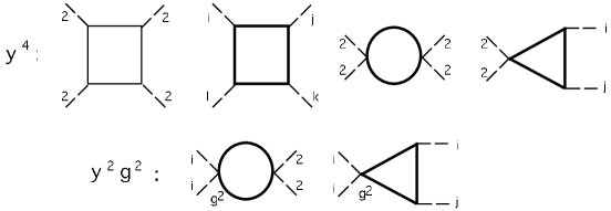
Figure 2: The 1PI diagrams needed for the 4-point function. For explanations see figure 1.

This is not yet the complete result for $\bar{\cal L}_{3}$; so far we have only integrated out the nonzero Matsubara frequency modes, which have masses of the order $\pi nT$. However there still remain particles with masses intermediate between this “superheavy” scale, and the light scale which is of order the magnetic mass of the transverse gauge bosons ($g^{2}T$). So we have to also integrate out the zero-Matsubara-frequency modes (called “heavy”) of the squarks, gauge bosons, and Higgs bosons, to an accuracy of $y^{2}$, $y^{4}$ or $g^{2}y^{2}$ in $\bar{\cal L}_{3}$. The diagrams that contribute are identical to the ones we already considered in deriving eq. (4); the difference is that the heavy particle masses are no longer given by $2\pi nT$, but rather the Debye mass.

To integrate out these remaining heavy modes, we must therefore determine their Debye masses, which consist of a tree-level part plus a thermal correction. For the left- and right-handed third-generation squarks in a vanishing background field ($H_{i}=0$) one finds [10]

$$m^{2}_{\tilde{q}_{L}} = m_{Q}^{2}+\frac{4g_{s}^{2}}{9}T^{2}+\frac{y_{t}^{2}+y_{b}^{2}}{6}T^{2}+\frac{g^{2}}{4}T^{2}+\frac{g^{\prime 2}}{108}T^{2}$$

$$m^{2}_{\tilde{t}_{R}} = m_{U}^{2}+\frac{4g_{s}^{2}}{9}T^{2}+\frac{y_{t}^{2}}{3}T^{2}+\frac{4g^{\prime 2}}{27}T^{2};$$

$$m^{2}_{\tilde{b}_{R}} = m_{D}^{2}+\frac{4g_{s}^{2}}{9}T^{2}+\frac{y_{b}^{2}}{3}T^{2}+\frac{g^{\prime 2}}{27}T^{2},$$ (5)

where the contributions from gauginos and charginos have been omitted, under the implicit assumption that they are so heavy that they decouple. (We have checked that including the latter contributions in the Debye masses has no qualitative effect on our subsequent numerical results.) In fact these are the only Debye masses we need because the squarks are the only particles in ${\cal L}_{3}$ whose tree-level couplings are proportional to $y$ or $y^{2}$. Ignoring the thermal loop corrections to these couplings, since they would only give two-loop corrections to $\bar{\lambda}_{3}$, the result of integrating out the heavy modes of the squarks is

$$\bar{\cal L}_{3}/T = {\cal L}_{3}/T+\frac{{\zeta_{t}}}{3M^{2}_{D_{t}}}|\mu\partial_{i}H_{1}+A_{t}\partial_{i}H_{2}|^{2}+\frac{{\zeta_{b}}}{3M^{2}_{D_{b}}}|\mu\partial_{i}H_{2}+A_{b}\partial_{i}H_{1}|^{2}$$ (6)

$$- {\zeta_{t}}M^{2}_{D_{t}}S^{t}_{+}-{\zeta_{b}}M^{2}_{D_{b}}S^{b}_{+}-D_{T}(|H_{1}|^{2}-|H_{2}|^{2})$$

$$- \frac{{\zeta_{t}}y_{t}^{2}}{4}\frac{M^{2}_{D_{t}}}{m_{\tilde{t}_{L}}m_{\tilde{t}_{R}}}(S^{t}_{-})^{2}-\frac{{\zeta_{b}}y_{b}^{2}}{4}\frac{M^{2}_{D_{b}}}{m_{\tilde{b}_{L}}m_{\tilde{b}_{R}}}(S^{b}_{-})^{2}$$

$$- \frac{{\zeta_{t}}g^{2}}{8}\frac{M_{D_{t}}}{m_{\tilde{t}_{L}}}\left(1+\frac{4g^{\prime 2}}{3g^{2}}\left(\frac{m_{\tilde{t}_{L}}}{m_{\tilde{t}_{R}}}-\frac{1}{4}\right)\right)S^{t}_{-}\left(|H_{1}|^{2}-|H_{2}|^{2}\right)$$

$$+ \frac{{\zeta_{b}}g^{2}}{8}\frac{M_{D_{b}}}{m_{\tilde{b}_{L}}}\left(1+\frac{2g^{\prime 2}}{3g^{2}}\left(\frac{m_{\tilde{b}_{L}}}{m_{\tilde{b}_{R}}}-\frac{1}{2}\right)\right)S^{b}_{-}\left(|H_{1}|^{2}-|H_{2}|^{2}\right),$$

where we defined $M_{D_{q}}\equiv m_{\tilde{q}_{L}}+m_{\tilde{q}_{R}}$, $\zeta_{q}\equiv 3y_{q}^{2}T/4\pi M_{D_{q}}$, $S^{t}_{\pm}\equiv|H_{2}|^{2}\pm M^{-2}_{D_{t}}|\mu H_{1}+A_{t}H_{2}|^{2}$, $S^{b}_{\pm}\equiv|H_{1}|^{2}\pm M^{-2}_{D_{b}}|\mu H_{2}+A_{b}H_{1}|^{2}$ and

$$D_{T}=\frac{g^{\prime 2}T}{8\pi}\left(2{m_{\tilde{t}_{R}}}-{m_{\tilde{q}_{L}}}-{m_{\tilde{b}_{R}}}\right).$$ (7)

The effective lagrangian so obtained is almost in the desired form, but it still depends on two Higgs doublets rather than one. At the phase transition, only one linear combination of the two is massless ($\Phi_{l}$), while the orthogonal direction is a heavy field ($\Phi_{h}$) which must also be integrated out. But since there are no self-couplings of the Higgs fields proportional to quark Yukawa couplings, this final step induces no new terms of the order of $y^{4}$ or $y^{2}g^{2}$ in ${\cal L}_{3}$; it is just a matter of projecting out the heavy field. Let the angle $\alpha$ describe the direction in field space whose eigenvalue in the temperature-dependent mass matrix of the two Higgs fields vanishes, at the phase transition temperature $T_{c}$:

$$\left(\begin{array}[]{c}H_{1}\\ H_{2}\end{array}\right)=\left(\begin{array}[]{cc}\cos\alpha&-\sin\alpha\\ \sin\alpha&\phantom{-}\cos\alpha\end{array}\right)\left(\begin{array}[]{c}\Phi_{l}\\ \Phi_{h}\end{array}\right).$$ (8)

Then the effect of integrating out the heavy field $\Phi_{h}$ is simply to replace $H_{1}$ by $\cos\alpha\;\Phi_{l}$ and $H_{2}$ by $\sin\alpha\;\Phi_{l}$.

Further let $m^{2}_{i,\rm eff}$ be the entries of the Higgs mass matrix, analogous to the tree-level $m^{2}_{i}$’s, but now corrected by the thermal loop diagrams. If we define the matrices

$${\bf m^{2}}=\left(\begin{array}[]{cc}m_{1}^{2}&m_{3}^{2}\\ m_{3}^{2}&m_{2}^{2}\\ \end{array}\right);\quad{\bf A}_{t}=\left(\begin{array}[]{cc}\mu^{2}&\mu A_{t}\\ \mu A_{t}&A^{2}_{t}\\ \end{array}\right);\quad{\bf A}_{b}=\left(\begin{array}[]{cc}A^{2}_{b}&\mu A_{b}\\ \mu A_{b}&\mu^{2}\\ \end{array}\right),$$ (9)

and

$${\bf P}_{b}=\left(\begin{array}[]{cc}1&0\\ 0&0\\ \end{array}\right);\quad{\bf P}_{t}=\left(\begin{array}[]{cc}0&0\\ 0&1\\ \end{array}\right);\quad{\bf P}_{3}=\left(\begin{array}[]{cc}1&0\\ 0&-1\\ \end{array}\right),$$ (10)

then ${\bf m^{2}_{\rm eff}}$ can be written as

$${\bf m^{2}_{\rm eff}} = {\bf m^{2}}+\Biggl{\{}-\frac{1}{2}{\eta_{t}}L_{f}\left\{{\bf P}_{t},\,{\bf m}^{2}\right\}-\frac{{\zeta_{t}}}{6M^{2}_{D_{t}}}\left\{{\bf A}_{t},\,{\bf m^{2}}\right\}$$ (11)

$$+ \left({\textstyle\frac{3}{4}}y^{2}_{t}T^{2}-{\eta_{t}}L_{B}(m^{2}_{Q}+m^{2}_{U})-{\zeta_{t}}M^{2}_{D_{t}}\right){\bf P}_{t}-\left({\eta_{t}}L_{B}+{\zeta_{t}}\right){\bf A}_{t}$$

$$+ (t\rightarrow b;\;m^{2}_{U}\rightarrow m^{2}_{D})\Biggr{\}}$$

$$- \left(\frac{g^{\prime 2}}{32\pi^{2}}L_{B}\,(2m^{2}_{U}-m^{2}_{D}-m^{2}_{Q})+D_{T}\right){\bf P}_{3}$$

$$\equiv {\bf m^{2}}+\frac{1}{2}\left\{\delta{\bf Z}_{T},{\bf m^{2}}\right\}+{\bf\Pi}_{T}(0),$$

where in the last line we made some definitions that will be useful later. The mixing angle is given by

$$\sin\alpha=\frac{-m^{2}_{1,\rm eff}}{(m^{4}_{1,\rm eff}+m^{4}_{3,\rm eff})^{1/2}}$$ (12)

at $T_{c}$, the temperature at which ${\rm Det}(m^{2}_{\rm eff})=0$. The anticommutators in eq. (11) arise due to wave function renormalization (rescaling $H_{i}$ so that the kinetic term in $\bar{\cal L}_{3}$ is properly normalized).

At one loop the gauge coupling $g_{3}$ is not renormalized by the Yukawa couplings. We checked this by computing the correction to $g_{3}$ from the correlator $\Phi_{l}\Phi_{l}A_{i}A_{i}$. The four relevant diagrams are shown in figure 3. After rescaling the fields to the canonical normalization, the direct contributions to this correlator are found to cancel those induced by wave function renormalization. So even after the heavy scale integration we have the tree level relation $\bar{g}^{2}_{3}=g^{2}T$.

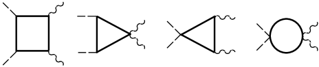
Figure 3: Diagrams contributing to the effective gauge coupling ${\bar{g}}_{3}$ in the heavy scale (zero-Matsubara-frequency) integration.

It is now straightforward to extract from eq. (6) the temperature-corrected quartic coupling of the light doublet $\Phi_{l}$. We find that

$${\bar{\lambda}_{3}\over\bar{g}^{2}_{3}} = {g^{2}+g^{\prime 2}\over 8g^{2}}\cos^{2}\!2\alpha$$ (13)

$$+ {3\ln 2\over 4\pi^{2}}\left({y_{t}^{4}\over g^{2}}\sin^{4}\!\alpha+\frac{g^{2}+g^{\prime 2}}{4g^{2}}y_{t}^{2}\cos 2\alpha\sin^{2}\!\alpha\right)$$

$$+ {3\ln 2\over 4\pi^{2}}\left({y_{b}^{4}\over g^{2}}\cos^{4}\!\alpha-\frac{g^{2}+g^{\prime 2}}{4g^{2}}y_{b}^{2}\cos 2\alpha\cos^{2}\!\alpha\right)$$

$$- \frac{3y_{t}^{4}}{16\pi g^{2}}\,\frac{M_{D_{t}}\,T}{m_{\tilde{t}_{L}}\,m_{\tilde{t}_{R}}}\,(S^{t}_{\alpha})^{2}-\frac{3y_{b}^{4}}{16\pi g^{2}}\,\frac{M_{D_{b}}\,T}{m_{\tilde{b}_{L}}\,m_{\tilde{b}_{R}}}\,(S^{b}_{\alpha})^{2}$$

$$- \frac{3y_{t}^{2}}{32\pi}\,\frac{T}{m_{\tilde{t}_{L}}}\left(1+\frac{4g^{\prime 2}}{3g^{2}}\left(\frac{m_{\tilde{t}_{L}}}{m_{\tilde{t}_{R}}}-\frac{1}{4}\right)\right)S^{t}_{\alpha}\cos 2\alpha$$

$$+ \frac{3y_{b}^{2}}{32\pi}\,\frac{T}{m_{\tilde{b}_{L}}}\left(1+\frac{2g^{\prime 2}}{3g^{2}}\left(\frac{m_{\tilde{b}_{L}}}{m_{\tilde{b}_{R}}}+\frac{1}{2}\right)\right)S^{b}_{\alpha}\cos 2\alpha$$

$$- \frac{y_{t}^{2}}{16\pi}\,\frac{g^{2}+g^{\prime 2}}{g^{2}}\,\frac{T}{M^{3}_{D_{t}}}\left(\mu^{2}\cos^{2}\alpha-A^{2}_{t}\sin^{2}\alpha\right)\cos 2\alpha,$$

$$+ \frac{y_{b}^{2}}{16\pi}\,\frac{g^{2}+g^{\prime 2}}{g^{2}}\,\frac{T}{M^{3}_{D_{b}}}\left(\mu^{2}\sin^{2}\alpha-A^{2}_{b}\cos^{2}\alpha\right)\cos 2\alpha,$$

where $S^{t}_{\alpha}\equiv\sin^{2}\!\alpha-M_{D_{t}}^{-2}(\mu\cos\alpha+A_{t}\sin\alpha)^{2}$ and $S^{b}_{\alpha}\equiv\cos^{2}\!\alpha-M_{D_{b}}^{-2}(\mu\sin\alpha+A_{b}\cos\alpha)^{2}$.

Eq. (13) gives the number that is directly bounded by the lattice results for the condition that the phase transition be sufficiently first order, eq. (2). However, the renormalization scale independence of the Lagrangian (6), is not yet apparent, and it contains undetermined parameters which must be expressed in terms of physical quantities. Once this is done, ${\cal L}_{3}$ becomes manifestly finite and independent of the scale $Q$.

3 Relation to the physical parameters

Figure 4: The tadpole diagrams needed for the 1-loop effective potential in the present approximation. The vertices marked by heavy circles (open circles) come from quartic terms of order $y^{2}$ ($g^{2}$), where one external Higgs field is replaced by its VEV.

The next step is to perform the zero-temperature renormalization to the same accuracy as we did at finite-temperature in order to express the parameters appearing in eq. (13) in terms of physical quantities, namely particle masses and the vacuum expectation values (VEV’s) of the two Higgs fields. The VEV’s are determined by minimizing the 1-loop effective potential, through the equations

$$\hskip-25.6073ptm^{2}_{1}+\tan\tilde{\beta}\;m^{2}_{3}+\frac{g^{2}+g^{\prime 2}}{4}(\tilde{v}^{2}_{1}-\tilde{v}^{2}_{2})\;+\;\frac{1}{2\tilde{v}_{1}}\frac{{\rm d}V_{1-\rm loop}}{{\rm d}\tilde{h}_{1}}=0,$$

$$\hskip-25.6073ptm^{2}_{2}+\cot\tilde{\beta}\;m^{2}_{3}-\frac{g^{2}+g^{\prime 2}}{4}(\tilde{v}^{2}_{1}-\tilde{v}^{2}_{2})\;+\;\frac{1}{2\tilde{v}_{2}}\frac{{\rm d}V_{1-\rm loop}}{{\rm d}\tilde{h}_{2}}=0,$$ (14)

where we have split the Higgs fields into CP-even and odd parts, $H_{i}=\tilde{h}_{i}+i\tilde{\chi}_{i}$, and $\tilde{v}_{i}=\langle H_{i}\rangle=\langle\tilde{h}_{i}\rangle$. The ratio of VEV’s is $\tan\tilde{\beta}=\tilde{v}_{2}/\tilde{v}_{1}$. Because we have not yet accounted for wave function renormalization at one loop, the $\tilde{v}_{i}$’s are not the physical VEV’s, defined to be $v_{i}=\langle h_{i}\rangle$, but the two sets of fields are related by matrix equations

$$\tilde{h}=({\bf Z}_{h})^{1/2}h\cong(1+{\textstyle\frac{1}{2}}\delta{\bf Z}_{h})h;\qquad\tilde{\chi}=({\bf Z}_{\chi})^{1/2}\chi\cong(1+{\textstyle\frac{1}{2}}\delta{\bf Z}_{\chi})\chi.$$ (15)

The matrices $\delta{\bf Z}$ can also be expressed in terms of the derivative of the 1-loop vacuum polarizations of the fields, $\delta{\bf Z}=({\rm d}{\bf\Pi}(p^{2})/{\rm d}p^{2})|_{p^{2}=0}={\bf\Pi}^{\prime}(0)$.

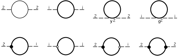
Figure 5: Diagrams contributing to the irreducible two point functions of the higgs fields in the broken phase. Vertices induced by spontaneous symmetry breaking do not contribute to the CP-odd two-point function. Again the indices on the external legs correspond to the top sector.

The minimization conditions (14) give us two equations for the three parameters $m^{2}_{i}$. To determine the third we must compute the physical mass of one of the Higgs bosons. A convenient choice is the CP-odd scalar, $A^{0}$. Its pole mass, $m_{A}$, is determined by

$${\rm Det}({\textstyle\frac{1}{2}}{\bf V}_{\!\!,\chi\chi}+{\bf\Pi}_{\chi}(m^{2}_{A})-m^{2}_{A})=0,$$ (16)

where ${\textstyle\frac{1}{2}}{\bf V}_{\!\!,\chi\chi}={\partial}^{2}V_{0}/{\partial}\chi_{i}{\partial}\chi_{j}$ is the tree-level mass matrix,

$${\textstyle\frac{1}{2}}{\bf V}_{\!\!,\chi\chi}={\bf m}^{2}+\frac{g^{2}+g^{\prime 2}}{4}(\tilde{v}^{2}_{1}-\tilde{v}^{2}_{2})\left(\begin{array}[]{cc}1&0\\ 0&-1\end{array}\right).$$ (17)

Of course an analogous expression could be used to relate the parameters to the CP-even Higgs masses, but the CP-odd sector is simpler because it contains a massless particle, the Goldstone boson. Rather than solving for the exact pole mass, we will renormalize at $p^{2}=0$, which means expanding ${\bf\Pi}_{\chi}(m^{2}_{A})\simeq{\bf\Pi}_{\chi}(0)+{\bf\Pi}^{\prime}_{\chi}(0)m^{2}_{A}$, so that ${\bf\Pi}_{\chi}(m^{2}_{A})+m^{2}_{A}$ becomes ${\bf\Pi}_{\chi}(0)-m^{2}_{A}{\bf Z}_{\chi}^{-1}$. After some manipulations using eq. (14) to eliminate the second term of (17), and using the explicit form of $dV_{1-\rm loop}/{\rm d}h_{i}$ (see the appendix), eq. (16) can be written as

$${\rm Det}\left(\begin{array}[]{cc}\Delta\tan\beta_{\chi}-m^{2}_{A}&-\Delta\\ -\Delta&\Delta\cot\beta_{\chi}-m^{2}_{A}\end{array}\right)=0,$$ (18)

where

$$\Delta\equiv-{m^{2}_{\chi 3}}+{\eta_{t}}\mu A_{t}F_{t}(Q)+{\eta_{b}}\mu A_{b}F_{b}(Q),$$ (19)

$m^{2}_{\chi 3}$ is the off-diagonal element of the symmetric matrix ${\bf m}^{2}_{\chi}\equiv{\bf m}^{2}+{\textstyle\frac{1}{2}}\{\delta{\bf Z}_{\chi},{\bf m}^{2}\}$, $F_{t,b}(Q)$ are the corrections due to squark loops,

$$F_{q}(Q)=\sum_{\pm}{\pm m^{2}_{\tilde{q}_{\pm}}\over m^{2}_{\tilde{q}_{+}}-m^{2}_{\tilde{q}_{-}}}\left(\ln\frac{Q^{2}}{m^{2}_{\tilde{q}_{\pm}}}+1\right),$$ (20)

and the squark masses are given by [11]

$$m^{2}_{\tilde{t}_{\pm}} = {\textstyle\frac{1}{2}}(m^{2}_{U}+m^{2}_{Q})+m^{2}_{t}+{\textstyle\frac{1}{4}}M^{2}_{Z}\cos 2\beta$$

$$\pm\sqrt{{\textstyle\frac{1}{4}}[m^{2}_{Q}-m^{2}_{U}+{\textstyle\frac{1}{2}}C_{t}M^{2}_{Z}\cos 2\beta]^{2}+m^{2}_{t}(A_{t}+\mu\cot\beta)^{2}};$$

$$m^{2}_{\tilde{b}_{\pm}} = {\textstyle\frac{1}{2}}(m^{2}_{D}+m^{2}_{Q})+m^{2}_{b}-{\textstyle\frac{1}{4}}M^{2}_{Z}\cos 2\beta$$ (21)

$$\pm\sqrt{{\textstyle\frac{1}{4}}[m^{2}_{Q}-m^{2}_{D}-{\textstyle\frac{1}{2}}C_{b}M^{2}_{Z}\cos 2\beta]^{2}+m^{2}_{b}(A_{b}+\mu\tan\beta)^{2}},$$

where $C_{t}=1-{\textstyle\frac{8}{3}}\sin^{2}\theta_{\rm W}$ and $C_{b}=1-{\textstyle\frac{4}{3}}\sin^{2}\theta_{\rm W}$.

To achieve the simple form (18) for the $A^{0}$ pole mass condition, we had to introduce the shifted angle $\beta_{\chi}$, defined by $\tan\beta_{\chi}\equiv v_{\chi 2}/v_{\chi 1}$, where $v_{\chi i}=(Z^{-1/2}_{\chi})_{ij}\tilde{v}_{j}$. The relation to the physical $\tan\beta$ is scale-independent: $\tan\beta_{\chi}=\tan\beta\left(1-{\textstyle\frac{1}{2}}\Delta Z_{11}+{\textstyle\frac{1}{2}}\Delta Z_{22}+\Delta Z_{12}\cot 2\beta\right),$ where $\Delta{\bf Z}={\bf Z}_{h}-{\bf Z}_{\chi}$. In the $\overline{\rm MS}$ subtraction scheme, which we are using throughout, the wave function renormalization matrices of the CP-odd and CP-even fields $\chi$ and $h$ are

$$\delta{\bf Z}_{\chi} = -{\eta_{t}}\;\ln\frac{Q^{2}}{m^{2}_{t}}\;{\bf P}_{t}-{\eta_{t}}H(m^{2}_{\tilde{t}_{+}},m^{2}_{\tilde{t}_{-}}){\bf A}_{t}\;+\;(t\rightarrow b);$$

$$\delta{\bf Z}_{h} = \delta{\bf Z}_{\chi}$$ (22)

$$+ {\eta_{t}}\left(\frac{2}{3}-\frac{m^{2}_{t}(m^{2}_{\tilde{t}_{+}}+m^{2}_{\tilde{t}_{-}})}{3m^{2}_{\tilde{t}_{+}}m^{2}_{\tilde{t}_{-}}}\right){\bf P}_{t}+\frac{{\eta_{t}}}{6}m_{t}\sin 2\theta_{t}\frac{m^{2}_{\tilde{t}_{+}}-m^{2}_{\tilde{t}_{-}}}{m^{2}_{\tilde{t}_{+}}m^{2}_{\tilde{t}_{-}}}{\bf P}_{A_{t}}$$

$$+ {\eta_{t}}\sin^{2}2\theta_{t}\left(H(m^{2}_{\tilde{t}_{+}},m^{2}_{\tilde{t}_{-}})-\frac{m^{2}_{\tilde{t}_{+}}+m^{2}_{\tilde{t}_{-}}}{12m^{2}_{\tilde{t}_{+}}m^{2}_{\tilde{t}_{-}}}\right){\bf A}_{t}$$

$$+ \frac{{\eta_{t}}}{24}M^{2}_{Z}\sin 2\beta\left(\frac{m^{2}_{\tilde{t}_{+}}+m^{2}_{\tilde{t}_{-}}}{m^{2}_{\tilde{t}_{+}}m^{2}_{\tilde{t}_{-}}}+C_{t}\cos 2\theta_{t}\frac{m^{2}_{\tilde{t}_{+}}-m^{2}_{\tilde{t}_{-}}}{m^{2}_{\tilde{t}_{+}}m^{2}_{\tilde{t}_{-}}}\right){\bf B}_{t}$$

$$+ \frac{3m_{t}}{128\pi^{2}}(g^{2}+g^{\prime 2})\sin 2\theta_{t}\left(\frac{m^{2}_{\tilde{t}_{+}}-m^{2}_{\tilde{t}_{-}}}{12m^{2}_{\tilde{t}_{+}}m^{2}_{\tilde{t}_{-}}}-C_{t}\cos 2\theta_{t}\left(H(m^{2}_{\tilde{t}_{+}},m^{2}_{\tilde{t}_{-}})-\frac{m^{2}_{\tilde{t}_{+}}+m^{2}_{\tilde{t}_{-}}}{12m^{2}_{\tilde{t}_{+}}m^{2}_{\tilde{t}_{-}}}\right)\right){\bf C}_{t}$$

$$+ (t\rightarrow b),$$

with ${\bf P}_{1,2}$ and ${\bf A}_{t,b}$ defined in (9 -10) and

$${\bf P}_{A_{t}}=\left(\begin{array}[]{cc}0&\mu\\ \mu&2A_{t}\end{array}\right)\;; {\bf P}_{A_{b}}\;=\;\left(\begin{array}[]{cc}2A_{b}&\mu\\ \mu&0\end{array}\right);$$ (27)

$${\bf B}_{t}=\left(\begin{array}[]{cc}0&-1\\ -1&2\tan\beta\end{array}\right)\;; {\bf B}_{b}\;=\;\left(\begin{array}[]{cc}2\cot\beta&-1\\ -1&0\end{array}\right)$$ (32)

$${\bf C}_{t}=\left(\begin{array}[]{cc}2\mu\cot\beta&A_{t}\cot\beta-\mu\\ A_{t}\cot\beta-\mu&-2A_{t}\end{array}\right)\;; {\bf C}_{b}=\left(\begin{array}[]{cc}-2A_{b}&A_{b}\tan\beta-\mu\\ A_{b}\tan\beta-\mu&2\mu\tan\beta\end{array}\right).$$ (37)

The squark mixing angles are defined by $\sin 2\theta_{t}=2m_{t}(A_{t}+\mu\cot\beta)/(m^{2}_{\tilde{t}_{+}}-m^{2}_{\tilde{t}_{-}})$ and $\cos 2\theta_{t}=(m^{2}_{U}-m^{2}_{Q}-{\textstyle\frac{1}{2}}C_{t}m^{2}_{Z}\cos 2\beta)/(m^{2}_{\tilde{t}_{+}}-m^{2}_{\tilde{t}_{-}})$ (for the bottom squarks let $t\to b$, $m^{2}_{U}\to m^{2}_{D}$ and $\cos\beta\leftrightarrow\sin\beta)$ and

$$H(m^{2}_{+},m^{2}_{-})\equiv\frac{1}{2(m^{2}_{+}-m^{2}_{-})}\left(\frac{m^{2}_{+}+m^{2}_{-}}{m^{2}_{+}-m^{2}_{-}}-\frac{2m^{2}_{+}m^{2}_{-}}{(m^{2}_{+}-m^{2}_{-})^{2}}\ln\frac{m^{2}_{+}}{m^{2}_{-}}\right).$$ (38)

Equation (18) has a vanishing eigenvalue corresponding to the Goldstone boson, and the nonzero eigenvalue is the mass of the $A^{0}$,

$$m^{2}_{A}=\frac{2\Delta}{\sin 2\beta_{\chi}}.$$ (39)

Our procedure for computing $m^{2}_{A}$ is somewhat more complicated than that of ref. [11] which parametrized all the effects of wave function renormalization in scale-dependent VEV’s, $v_{i}(Q^{2})$, whereas we take the VEV’s and hence $\tan\beta$ to be physical, scale-independent quantities. Our answer reduces to theirs if we neglect the wave function renormalization effects, i.e. by taking $\beta_{\chi}\to\beta$ and $m^{2}_{\chi 3}\to m^{2}_{3}$.

The solution (39) allows the lagrangian mass parameter $m^{2}_{3}$ to be expressed in terms of $m^{2}_{A}$. Then, having found $m^{2}_{3}$, the other elements $m_{1,2}^{2}$ are determined by the minimization conditions (14). It is convenient however, to give the results in terms of the scaled quantity $m^{2}_{\chi 3}$ (see below eq. (19)). We find:

$${\bf m}^{2}_{\chi}(Q) = {\textstyle\frac{1}{2}}m^{2}_{A}\sin 2\beta_{\chi}\left(\begin{array}[]{cc}\tan\beta_{\chi}&-1\\ -1&\cot\beta_{\chi}\end{array}\right)$$

$$+ {\eta_{t}}F_{t}(Q){\bf A}_{t}+{\eta_{b}}F_{b}(Q){\bf A}_{b}+{\eta_{t}}G_{t}(Q){\bf P}_{t}+{\eta_{t}}G_{b}(Q){\bf P}_{b}$$

$$- {\textstyle\frac{1}{2}}M^{2}_{Z}(Z^{h}_{11}\cos^{2}\beta-Z^{h}_{22}\sin^{2}\beta)({\bf P}_{b}Z^{\chi}_{11}-{\bf P}_{t}Z^{\chi}_{22})$$

$$+ {\textstyle\frac{3}{128\pi^{2}}}(g^{2}+g^{\prime 2})D(Q){\bf P}_{3},$$ (43)

where

$$G_{q}(Q)\equiv\sum_{\pm}m^{2}_{\tilde{q}_{\pm}}\left(\ln{Q^{2}\over m^{2}_{\tilde{q}_{\pm}}}+1\right)-2m^{2}_{q}\left(\ln\frac{Q^{2}}{m^{2}_{q}}+1\right)$$ (44)

and the other new function, coming from the tadpoles of the $g^{2}|\tilde{q}|^{2}|H|^{2}$ terms of eq. (3), is given by

$$D(Q) = \sum_{\pm}m^{2}_{\tilde{t}\scriptscriptstyle\pm}\left(\ln(Q^{2}/m^{2}_{\tilde{t}\scriptscriptstyle\pm})+1\right)-\sum_{\pm}m^{2}_{\tilde{b}\scriptscriptstyle\pm}\left(\ln(Q^{2}/m^{2}_{\tilde{b}\scriptscriptstyle\pm})+1\right)$$ (45)

$$+C_{t}(m^{2}_{Q}-m^{2}_{U}+{\textstyle\frac{1}{2}}C_{t}M^{2}_{Z}\cos 2\beta)F_{t}(Q)$$

$$-C_{b}(m^{2}_{Q}-m^{2}_{D}-{\textstyle\frac{1}{2}}C_{b}M^{2}_{Z}\cos 2\beta)F_{b}(Q).$$

These are all the expressions needed to solve for the entries of the effective mass matrix ${\bf m}^{2}_{\rm eff}$. It is convenient to do so in terms of the scaled matrix ${\bf m}_{\chi}$, using eq. (4):

$${\bf m}^{2}_{\rm eff}={\bf m}^{2}_{\chi}+\frac{1}{2}\{\delta{\bf Z}_{T}-\delta{\bf Z}_{\chi},{\bf m}^{2}_{\chi}\}+{\bf\Pi}_{T}(0),$$ (46)

where $\delta{\bf Z}_{T}$ and ${\bf\Pi}_{T}(0)$ were defined in (11). The difference between the wave function renormalization matrices at finite and at zero temperature is finite and scale-independent, as it must be. Moreover, the $Q$-dependence appearing in ${\bf m}_{\chi}^{2}$ (43) is precisely what is needed to cancel that coming from ${\bf\Pi}_{T}(0)$ at the accuracy to which we are working, so that the matrix ${\bf m}^{2}_{{\rm eff}}$ and hence the angle $\cos^{2}\!\alpha$ are scale-independent. The result is

$${\bf m}^{2}_{\rm eff} = {\bf m}^{2}_{\chi}(T)+\Biggl{\{}(2{\eta_{t}}c_{B}-{\zeta_{t}}){\bf A}_{t}+\left({\textstyle\frac{3}{4}}y_{t}^{2}T^{2}+2{\eta_{t}}c_{B}(m^{2}_{Q}+m^{2}_{U})-{\zeta_{t}}M^{2}_{D_{t}}\right){\bf P}_{t}$$ (47)

$$+ \frac{1}{2}\left({\eta_{t}}H(m^{2}_{\tilde{t}_{+}},m^{2}_{\tilde{t}_{-}})-\frac{{\zeta_{t}}}{3M^{2}_{D_{t}}}\right)\left\{{\bf A}_{t},{\bf m^{2}}\right\}+\frac{1}{2}{\eta_{t}}\left(2c_{F}+\ln\frac{T^{2}}{m^{2}_{t}}\right)\left\{{\bf P}_{t},{\bf m^{2}}\right\}$$

$$+ (t\rightarrow b;\;m^{2}_{U}\rightarrow m^{2}_{D})\Biggr{\}}+\left(\frac{g^{\prime 2}}{16\pi^{2}}c_{B}\,(2m^{2}_{U}-m^{2}_{D}-m^{2}_{Q})-D_{T}\right){\bf P}_{3},$$

where the matrix ${\bf m}^{2}_{\chi}(T)$ is as in (43) but with $Q=T$, and we define $c_{B}\equiv\ln 4\pi-\gamma_{E}$ and $c_{F}\equiv\ln\pi-\gamma_{E}$. To one-loop accuracy, it suffices to use the tree level expression for ${\bf m}^{2}$ appearing in the anticommutators, which in terms of physical parameters is given by

$${\bf m}^{2}_{\rm tree}={\textstyle\frac{1}{2}}m^{2}_{A}\sin 2\beta\left(\begin{array}[]{cc}\tan\beta&-1\\ -1&\cot\beta\end{array}\right)-{\textstyle\frac{1}{2}}M^{2}_{Z}\cos 2\beta\;{\bf P}_{3}.$$ (48)

In the next section we will identify the regions of parameter space where baryogenesis is allowed. One must check whether these parameters are in fact compatible with other constraints, including the experimental lower limit on the mass of the lightest Higgs boson $h^{0}$, whose tree level expression vanishes when $\tan\beta=1$. Since we will find that low values of $\tan\beta$ are relevant for electroweak baryogenesis, it is important to include loop corrections to $m_{h^{0}}$, which can be large. The pole mass of the $h^{0}$ is determined similarly to eq. (16):

$${\rm Det}({\textstyle\frac{1}{2}}{\bf V}_{\!\!,hh}-{\bf\Pi}_{h}(m^{2}_{h})-m^{2}_{h})=0,$$ (49)

where

$${\textstyle\frac{1}{2}}{\bf V}_{\!\!,\chi\chi}={\bf m}^{2}+\frac{g^{2}+g^{\prime 2}}{4}\left(\begin{array}[]{cc}3\tilde{v}^{2}_{1}-\tilde{v}^{2}_{2}&-2\tilde{v}_{1}\tilde{v}_{2}\\ -2\tilde{v}_{1}\tilde{v}_{2}&3\tilde{v}^{2}_{2}-\tilde{v}^{2}_{1}\end{array}\right).$$ (50)

Expanding the 2-point function $\Pi_{h}(m^{2}_{h})$ and performing other manipulations similar to the CP-odd case, eq. (49) can be put into the form

$${\rm Det}({\bf M}^{2}(\beta)-m^{2}_{h})=0,$$ (51)

where

$${\bf M^{2}}(\beta) = \frac{1}{2}m^{2}_{A}\sin 2\beta_{\chi}\left(\begin{array}[]{cc}\tan\beta_{\chi}&-1\\ -1&\cot\beta_{\chi}\end{array}\right)+{\textstyle\frac{1}{2}}M^{2}_{Z}\sin 2\beta\left(\begin{array}[]{cc}\cot\beta&-1\\ -1&\tan\beta\end{array}\right)$$

$$+ \frac{{\eta_{t}}}{2}\sin^{2}2\theta_{t}\;I(m^{2}_{\tilde{t}_{+}}/m^{2}_{\tilde{t}_{-}})\;{\bf A}_{t}+2{\eta_{t}}m^{2}_{t}\ln\frac{m^{2}_{\tilde{t}_{+}}m^{2}_{\tilde{t}_{-}}}{m^{4}_{t}}{\bf P}_{t}$$

$$+ {\eta_{t}}m_{t}\sin 2\theta_{t}\ln\frac{m^{2}_{\tilde{t}_{+}}}{m^{2}_{\tilde{t}_{-}}}{\bf P}_{A_{t}}+({\textstyle\frac{1}{2}}M^{2}_{Z}\sin 2\beta\;\delta Z^{h}_{22}+\Pi^{t}_{1}(Q)){\bf B}_{t}$$

$$+ \Pi^{t}_{2}\;{\bf C}_{t}\;\;+\;\;(t\rightarrow b),$$ (57)

with

$$I(r)=2-\frac{r+1}{r-1}\ln r$$ (58)

and

$$\Pi^{q}_{1}(Q) = \frac{1}{2}\eta_{q}M^{2}_{Z}\sin 2\beta\left(\ln\frac{Q^{2}}{m_{\tilde{q}_{+}}m_{\tilde{q}_{-}}}+\frac{1}{2}C_{q}\cos 2\theta_{q}\ln\frac{m^{2}_{\tilde{q}_{+}}}{m^{2}_{\tilde{q}_{-}}}\right);$$

$$\Pi^{q}_{2} = \frac{3m_{t}}{256\pi^{2}}(g^{2}+g^{\prime 2})\;\sin 2\theta_{t}\left(\ln\frac{m^{2}_{\tilde{t}_{+}}}{m^{2}_{\tilde{t}_{-}}}-C_{t}\cos 2\theta_{t}I(m^{2}_{\tilde{t}_{+}}/m^{2}_{\tilde{t}_{-}})\right).$$ (59)

It is easy to see that the $Q$-dependence in (57) due to $\Pi^{t}_{1}(Q)$ ($\Pi^{b}_{1}(Q)$) exactly cancels that of $\delta Z^{h}_{22}$ ($\delta Z^{h}_{22}$). We verified that the solution of eq. (51), giving $m^{2}_{h}$ as a function of $\tan\beta$, agrees with previous results [12].

4 Results

Having completely determined the quantity $\bar{\lambda}_{3}/\bar{g}^{2}_{3}$ in terms of the physical parameters, we now turn to the question of whether the baryons created during the electroweak phase transition can be preserved from subsequent sphaleron interactions within the MSSM. Specifically, for what values of the physical parameters does $\bar{\lambda}_{3}/\bar{g}^{2}_{3}$ satisfy the bound (2)? A priori there seems to be no simple, analytic answer to this question. No single term among the many loop corrections in eq. (11) could be identified as being dominant over the others, and furthermore the parameter space is large: $\tan\beta$, $m_{A^{0}}$, $m^{2}_{Q}$, $m^{2}_{U}$, $m^{2}_{D}$, $\mu$, $A_{t}$, $A_{b}$. We therefore chose to do a Monte Carlo search of this space for values which satisfy the constraint (2).

The preceding list of parameters does not include the gauge or Yukawa coupling constants because these can be defined through the tree level relations, $(g^{2}+g^{\prime 2})/g^{2}=m^{2}_{Z}/m^{2}_{W}$, $y^{2}_{t}=m^{2}_{t}/v^{2}\sin^{2}\!\beta$ and $y^{2}_{b}=m^{2}_{b}/v^{2}\cos^{2}\!\beta$. For the gauge couplings this is a consequence of the vanishing of the Yukawa contributions to the beta function at one loop, and our neglect of the difference between the pole masses and the masses defined at zero external momentum. As for the Yukawa couplings, these appear only in loop corrections for us, so to one-loop accuracy it is consistent to use their tree-level values.

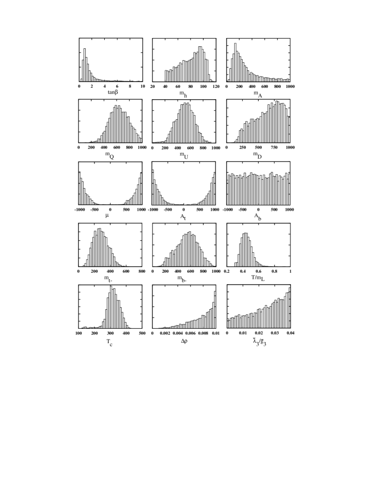
Figure 6: The projected distributions of the data satisfying the sphaleron washout bound (2) obtained from the Monte Carlo run described in the text. Units are GeV.

For the Monte Carlo search we found it convenient to take as independent parameters those listed in Table I, which shows the ranges over which they were varied. The massive parameters were allowed to be as large as 1 TeV. These MC-generated sets were subjected to various constraints. The lower limits for the pseudoscalar mass $m_{A^{0}}$ and the squark masses were taken to be 20 GeV and 45 GeV, respectively, and we used the recent top quark mass measurement of $m_{t}=175$ GeV [13]. We further required that the squark masses and mixings be consistent with deviations of the $\rho$ parameter from unity of less than 0.01 (see ref. [6]). Specifically, the contributions from the top-bottom quark and squark splittings as computed in ref. [14], including squark mixing effects, were constrained to satisfy $\Delta\rho(t,b)+\Delta\rho(\tilde{t},\tilde{b})<0.01$. Finally, the accepted data were required to satisfy the baryogenesis constraint (2) and stability of the potential ($\bar{\lambda}_{3}>0$). The distributions of the parameters within this set, as well as histograms of derived quantities like the squark and Higgs masses, $\bar{\lambda}_{3}/\bar{g}^{2}_{3}$, and the critical temperature, are shown in figure 6. As a rough indication of how special the 5,600 accepted sets were among all possibilities, including some with unphysical masses or couplings, we needed 40 million trials to generate them. The baryogenesis-allowed cases thus constitute approximately 0.014 percent of the full parameter space.

$\tan\beta$	$m_{A^{0}}$	$m^{2}_{Q,U,D}$	$\mu,A_{t},A_{b}$
0.4	20 GeV	0	$-$1 TeV
10	1 TeV	1 TeV2	-1 TeV

Table 1: Minimum and maximum values used in the Monte Carlo of the parameters.

One of the most striking features of the distributions is that $\tan\beta$ is sharply peaked near unity and falls to a small but constant value of approximately $10^{-2}$ of the maximum frequency. Thus it would appear that small values of $\tan\beta$ are strongly favored by our results. This is somewhat misleading however, because there is a strong correlation between $\tan\beta$ and $m_{A^{0}}$, as shown in figure 7. The probability of getting large values of $\tan\beta$ is very much dependent upon $m_{A^{0}}$. If for whatever reason it became known that $m_{A^{0}}$ was in the region of $40-120$ GeV, the distribution of $\tan\beta$ would be much flatter than is shown in figure 6, with very large values being almost as likely as small ones. This correlation is also evident in the distribution for $m_{A^{0}}$, which jumps up at small values, due to the enlargement of allowed parameters in the direction of increasing $\tan\beta$.

Moreover the distributions for $\mu$ and $A_{t}$ show a very clear preference for large mixings. There are allowed parameters also close to $\mu,A_{t}=0$, but those corresponding to large mixing are much more numerous. The large squark mixing angles are also correlated with the rather large average value of 300 GeV of the critical temperature. Due to the smallness of the coupling $y_{b}$, the bottom squark sector corrections are small, which shows in the flatness of the $A_{b}$-distribution.

Figure 7: The baryogenesis-allowed points in the $\tan\beta$-$m_{A^{0}}$ plane. The sphaleron bound (2) pushes the solutions close to axes; the region away from the axes is populated by points with $\bar{\lambda}_{3}/\bar{g}^{2}_{3}\gg 0.04$, in violation of the bound. Units of $m_{A^{0}}$ are GeV.

The other variables also display certain preferences. The lighter squark masses peak at 260 GeV and 480 GeV, showing some preference for a moderately light top squark, though not as light as that advocated by the perturbative study in reference [8]. Furthermore the probability for $m^{2}_{U}$ to be negative, suggested in ref. [7] as an optimum choice for strengthening the phase transition, appears to be quite small. The mass of the lightest Higgs boson, $m_{h^{0}}$, is in the range of 40 GeV (the experimental lower limit we imposed) to 130 GeV. The $\Delta\rho$-distribution [14] sharply increases for large $\Delta\rho$, showing the severity of this constraint on the data. It is important to note, however, that large squark mixing angles make it much easier to satisfy the $\rho$-parameter constraint. Finally, the parameter characterizing the strength of the phase transition, $\bar{\lambda}_{3}/\bar{g}^{2}_{3}$, is monotonically increasing, reflecting the difficulty of getting a strongly first order transition.

Figure 8: The density distributions in ($m_{Q}/\pi T_{c},m_{U}/\pi T_{c}$) and ($m_{Q}/\pi T_{c},m_{U}/\pi T_{c}$) planes. Dotted lines show the borders of the accepted regions $m_{Q,U,D}/\pi T_{c}<1$.

There are two further constraints that we imposed on our accepted data sets. First, care must be taken to ensure that the finite-temperature perturbative expansion is not breaking down where we need it. In particular, the thermal squark loop contributions as written in eq. (4) are only correct if the zero-Matsubara-frequency (“heavy”) modes are much lighter than the nonzero ones (“superheavy”), which requires that $m_{Q,U,D}<2\pi T$. We checked that the squark contribution to the quartic piece of ${\cal L}_{3}$ in eq. (4) differs from the exact result (not expanded in $m^{2}/T^{2}$) by less than 5% for $m_{Q,U,D}<\pi T$ and by a factor of $\sim 2$ at $m_{Q,U,D}\sim 2\pi T$. We imposed the more stringent cut of $m_{Q,U,D}<\pi T_{c}$ on our data, which reduced the size of the sample roughly by a factor of six. The effect of these cuts is clearly seen in figure 8, where we show the density plots of the distributions $m_{Q,U,D}/\pi T_{c}$, based on a separate run with the constraint $m_{Q,U,D}<2\pi T_{c}$.

Second, one has to insure the validity of the heavy scale perturbation theory. A typical expansion parameter for integrating out the heavy modes is $\zeta_{t}=3y^{2}_{t}T/4\pi M_{D_{t}}$, which should not become too large; we required that $T/m<1$ for all Debye masses m. From the distribution for $T/m_{\tilde{t}_{L}}$ in figure 6 one sees however that the other cuts (in particular the requirement $m_{Q,U,D}<\pi T_{c}$) already confine the heavy scale expansion parameters to the range needed to insure $\zeta<1$. This is partly because we did not consider negative values for $m^{2}_{U}$ in the present work.

Clearly, making these consistency cuts can lead us to neglect parameter values that might actually be acceptable for electroweak baryogenesis. However it is difficult to consistently implement the dimensional reduction program except for the relatively light squark masses that pass our cuts, or in the opposite limit of $m_{Q,U,D}\gg 2\pi T_{c}$ where the heavy modes decouple, since only then is there a clear hierarchy between the superheavy and heavy scales. (Of course the same problem exists in the purely perturbative effective potential approach.) A naive way to interpolate between these limits would be to replace the $m^{2}/T^{2}$ expansions with the exact expressions for the corresponding finite temperature integrals. While not quite rigorous, this might provide a reasonable approximation to the exact result. An investigation along these lines is in progress.

5 Conclusions

We examined the strength of the first order electroweak phase transition in the MSSM with respect to the prospects for safeguarding electroweak baryogenesis from washout by residual sphaleron interactions, finding rather encouraging results. Although our calculations were perturbative, the method—computing the three-dimensional finite-temperature effective action of the light Higgs and gauge fields at the phase transition—enabled us to take advantage of nonperturbative results that have been obtained from lattice gauge theory computations. This is therefore the first study of the phase transition in the MSSM that can claim to be free from the infrared divergences that make the usual perturbative calculations untrustworthy. Indeed, we find that the results of these two distinct approaches disagree.

The most serious constraint on electroweak baryogenesis in the MSSM, seen also in the earlier investigations [6]-[8], seems to be the bias toward small values of $\tan\beta\mbox{\raisebox{-2.58334pt}{~{}$\stackrel{{\scriptstyle<}}{{\sim}}$~{}}}2$. But in our approach this bias is very different from a prohibition on large values of $\tan\beta$; in fact such values are not ruled out, but they must appear in conjunction with low values ($40-120$ GeV) of the $A^{0}$ boson mass, as is clear from our figure (7). Since there is no intrinsically “correct” integration measure for the space of all parameters in the MSSM, the large $\tan\beta$ possibility can hardly be considered less natural, even if it comprised a smaller subset of our Monte Carlo results. If the limit on $m_{A^{0}}$ should be improved such as to exclude this region, then it will become a question of whether $\tan\beta\mbox{\raisebox{-2.58334pt}{~{}$\stackrel{{\scriptstyle<}}{{\sim}}$~{}}}1.5$ is viable.

There is one important caveat to our conclusions: as emphasized in [9], the approach used here assumes that the only light degrees of freedom at the phase transition are the transverse gauge bosons and a single linear combination of the two Higgs fields. It is possible that other fields which are generically heavy happen to also be light for special parameter values–for example, the Debye masses of the squarks can vanish if $m^{2}_{Q,U,D}<0$. In such cases we can say nothing until the lattice computations are redone to take into account these potential new sources of infrared divergences.

Note Added

Soon after this paper was completed, we received two articles where the same problem was considered. Losada [16] derived the dimensionally reduced lagrangian, keeping also the $g^{4}$-corrections (but setting $g^{\prime}=0$). Laine [17] made a complete analysis in an approximation similar to ours. Where comparison is possible, our results are in good agreement.

Appendix A Appendix

Here we give the derivatives of the effective potential and the zero-momentum limits of 2-point functions, which were necessary to derive, but not to finally express, the relevant quantities in the body of the text.

$$\frac{1}{2v_{1}}\frac{{\rm d}V_{1}}{{\rm d}h_{1}} = -{\eta_{t}}(\mu^{2}+\mu A_{t}\tan\beta)F_{t}(Q)-{\eta_{b}}(A^{2}_{b}+\mu A_{b}\tan\beta)F_{b}(Q)$$

$$-{\eta_{b}}G_{b}(Q)-{\textstyle\frac{3}{128\pi^{2}}}(g^{2}+g^{\prime 2})D(Q)$$

$$\frac{1}{2v_{2}}\frac{{\rm d}V_{1}}{{\rm d}h_{2}} = -{\eta_{t}}(A_{t}^{2}+\mu A_{t}\cot\beta)F_{t}(Q)-{\eta_{t}}(\mu^{2}+\mu A_{b}\cot\beta)F_{b}(Q)$$ (60)

$$-{\eta_{t}}G_{t}(Q)+{\textstyle\frac{3}{128\pi^{2}}}(g^{2}+g^{\prime 2})D(Q),$$

with $F_{q}(Q)$ defined in (20), $G_{q}(Q)$ in (44) and $D(Q)$ in (45). The two-point function of the CP-odd sector at the zero momentum is given by

$${\bf\Pi}(0)^{\chi} = -{\eta_{t}}G_{t}(Q){\bf P}_{t}-{\eta_{t}}F_{t}(Q){\bf A}_{t}\;+\;(t\rightarrow b)$$ (61)

$$-{\textstyle\frac{3}{128\pi^{2}}}(g^{2}+g^{\prime 2})D(Q){\bf P}_{3},$$

with ${\bf P}_{i}$ defined in (10). In the CP-even sector we find the result

$${\bf\Pi}(0)^{h} = {\bf\Pi}(0)^{\chi}$$ (62)

$$+ \frac{{\eta_{t}}}{2}\sin^{2}2\theta_{t}\;I(m^{2}_{\tilde{t}_{+}}/m^{2}_{\tilde{t}_{-}})\;{\bf A}_{t}+\eta_{t}m_{t}\sin 2\theta_{t}\;\ln\frac{m^{2}_{\tilde{t}_{+}}}{m^{2}_{\tilde{t}_{-}}}{\bf P}_{A_{t}}$$

$$+ 2\eta_{t}\;m^{2}_{t}\ln\frac{m^{2}_{\tilde{t}_{+}}m^{2}_{\tilde{t}_{-}}}{m^{4}_{t}}{\bf P}_{t}+\Pi^{t}_{1}(Q){\bf B}_{t}+\Pi^{t}_{2}\;{\bf C}_{t}$$

$$+ (t\rightarrow b),$$

with ${\bf P}_{Aq}$, ${\bf B}_{i}$ and ${\bf C}_{i}$ defined in (37), $I(r)$ in (58) and $\Pi^{q}_{i}$ in (59).