UFTP preprint 414/1996

IR-Renormalon Contribution to the
Polarized Structure Function $g_{1}$

M. Meyer-Hermann^†, M. Maul^†, L. Mankiewicz^††, E. Stein^†, and A. Schäfer^†

^†Institut für Theoretische Physik, J. W. Goethe Universität Frankfurt,

Postfach 11 19 32, D-60054 Frankfurt am Main, Germany

^††Institut für Theoretische Physik, TU-München, D-85747 Garching, Germany

Abstract: An estimation of the higher twist contribution to the polarized nonsinglet structure function $g_{1}$ is given. Its first moment is generally assumed to be small but this could be due to a cancellation of its contribution in different Bjorken-$x$ ranges. We estimate the magnitude of $g_{1}^{tw4}$ as a function of $x$ in the framework of the renormalon method. The calculated higher-twist-correction to $g_{1}$ turn out to be in fact small for all $x$ values. The correction to the determination of the nonsinglet matrix element $d_{NS}^{(2)}$ from data for transversely nucleon polarization due to the calculated higher twist effects is of order $10\%$.

Recently the E143 collaboration measured the transverse polarized structure function for proton and neutron [1] and obtained a first approximate result for the nonsinglet twist-3 matrix element $d_{NS}^{(2)}$. This analysis relies on the assumption that the higher twist contributions to $g_{1}^{p-n}$ are negligible. This experimental result is in strong disagreement with predictions from lattice calculations [2], and in marginal agreement with predictions from QCD sum rule calculations [3] such that possible sources of error have to be looked into very carefully. One such uncertainty in the experimental determination of $d_{NS}^{(2)}$ is the size of higher twist contributions to $g_{1}^{p-n}$. Theoretically they could be large even if they give only a small contribution to the first moment of $g_{1}^{p-n}$, for example if the latter is due to a cancellation of twist-4 contributions from different Bjorken-$x$ regions with different signs.

To know the size of the higher twist contributions is also very important for recent attempts to obtain $\Delta G(x)$ from the $Q^{2}$-dependence of $g_{1}(x,Q^{2})$ [4, 5]. We present a renormalon estimate showing that there are in fact cancelations for the first moment of $g_{1}^{tw4}$. The higher twist contributions to $g_{1}(x,Q^{2})$ are nevertheless small, such that the mentioned analysis of experimental data is valid.

Neglecting higher twist contributions the moments of the nonsinglet polarized structure function $g_{1}(x,Q^{2})$ can, in the framework of operator product expansion, be identified with the twist-2 nonsinglet operator matrix elements $A_{g_{1},n}$ (we abbreviate $g_{1}(x,Q^{2}):=g_{1}^{p}(x,Q^{2})-g_{1}^{n}(x,Q^{2})$):

$$M_{g_{1},n}(Q^{2}) = \int_{0}^{1}dx\;x^{n-1}g_{1}(x,Q^{2})$$ (1)

$$= C_{g_{1},n}\left(\frac{Q^{2}}{\mu^{2}},a_{s}\right)A_{g_{1},n}(\mu^{2})$$

Here we introduced the factorization scale $\mu$ and the Wilson-coefficient $C_{n}$. $a_{s}$ is the strong coupling, defined by $a_{s}:=\frac{g^{2}}{(4\pi)^{2}}$. Higher twist operator matrix elements are not written.

To estimate higher twist contributions to eq. (1) we use the renormalon-method [6]. The forward Compton-scattering-amplitude is calculated in the Borel-plane with an effective gluon propagator, taking only one gluon exchange into account. In the Landau gauge the effective gluon propagator resums arbitrary many quark loop insertions in the gluon line, which is an exact procedure in QED. The gluon propagator reads in the Borel representation [7]:

$${\cal B}_{1/a_{s}}[a_{s}D^{ab}_{\mu\nu}(k)](u)\;=\;\delta^{ab}\frac{g_{\mu\nu}-\frac{k_{\mu}k_{\nu}}{k^{2}}}{k^{2}}\left(\frac{\mu^{2}e^{-C}}{-k^{2}}\right)^{\beta_{0}u}\;,$$ (2)

$C$ corrects for the renormalization scheme dependence ($C=-\frac{5}{3}$ for $\overline{MS}$-scheme) and $u$ is the Borel transformation parameter. In QCD the restriction to one gluon exchange is an exact procedure in the large $N_{F}$-limit [8, 9, 10], where $N_{F}$ is the number of quark-flavors. The next-to-leading $N_{F}$-order terms are approximated by naive-nonabelianization (NNA) [7, 11, 12, 13], which means to replace the one loop beta-function of QED by the QCD beta-function $\beta_{0}=11-\frac{2}{3}N_{F}$ and corresponds to the replacement $N_{F}\rightarrow N_{F}-\frac{33}{2}$. The quality of this approximation has to be checked by comparing the NNA-perturbative-coefficients with the known exact ones.

The IR-renormalon-poles lead to an factorial growth of the perturbative series, which has to be interpreted as an asymptotic expansion. In agreement with the general theory of asymptotic series it has to be truncated after the minimal term, which determines the best accuracy which can be achieved using perturbative expansion. As its $Q^{2}$ dependence is power-like, it has been suggested to use it as an estimate of higher-twist contributions. Despite the fact that the conceptual basis for this approach is controversial [14], the procedure has given previously reasonable estimates [15, 16, 17] and is much simpler than genuine higher twist estimates due to lattice or QCD sum rules calculations.

Finally, let us mention that there are two popular methods of computing the renormalon ambiguity in the QCD perturbative series. Apart from the Borel-transformed propagator (2) one can use a gluon propagator with a small gluon mass $\lambda^{2}$. The coefficient of the $n$-th renormalon pole is the same as the coefficient of the $\lambda^{2n}ln(\lambda^{2})$-term in the small gluon-mass approach. Despite seemingly different physical meaning, both methods are exactly equivalent [13, 18].

The paper is organized as follows: first the Wilson-coefficient for all moments of $g_{1}$ are calculated in the NNA approximation using the Borel-transformed gluon-propagator. Then the perturbative coefficients are calculated in the NNA approximation and are compared to known exact values. Next the IR renormalon ambiguity is calculated and used for an estimate of the twist-4 corrections to the polarized structure function. As the calculation is done for all moments, the twist-4 corrections are given as a function of Bjorken-$x$. Finally we give a phenomenological analysis of the twist-4 contribution.

The forward Compton scattering amplitude corresponding to the polarized structure function $g_{1}$ reads after an expansion in $\omega=1/x$:

$$T_{\mu\nu}^{g_{1}}\;=\;2i\varepsilon_{\mu\nu\lambda\rho}\frac{q^{\lambda}s^{\rho}}{p\cdot q}\sum_{\stackrel{{\scriptstyle n=1}}{{\rm odd}}}^{\infty}C_{g_{1},n}\left(\frac{Q^{2}}{\mu^{2}},a_{s}\right)A_{g_{1},n}(\mu^{2})\,\omega^{n}$$ (3)

We have computed the one-gluon-exchange diagrams contributing to deep inelastic lepton-nucleon scattering using the effective gluon propagator (2).

The result in the Borel plane is expanded in $\omega$ and compared to eq. (3) to read off the Borel transformed Wilson coefficient. Note that the Borel transformation of eq. (3) is given by a similar expression with the Borel transformed Wilson coefficient on the right hand side. The resulting antisymmetric part is (we use the notation of Muta [19] and $s=\beta_{0}u$):

$${\cal B}_{\frac{1}{a_{s}}}\!\left[C_{g_{1},n}\left(\frac{Q^{2}}{\mu^{2}},a_{s}\right)\right]\!(u) \!\!\!=\!\!\! -2C_{F}\left(\frac{\mu^{2}e^{-C}}{Q^{2}}\right)^{s}$$ (4)

$$\Bigg{\{}\frac{1}{s}\bigg{[}\frac{\Gamma(s+n)}{\Gamma(1+s)\Gamma(n)}\left(\frac{1}{(s+n)(1+s+n)}+\frac{1}{1+s+n}+\frac{1}{2}\right)$$

$$\hskip 17.07164pt-\sum_{k=1}^{n}\frac{\Gamma(s+k)}{\Gamma(1+s)\Gamma(k)}\left(\frac{1}{s+k}+\frac{1}{1+s+k}\right)\bigg{]}$$

$$+\frac{2}{1-s}\bigg{[}\frac{\Gamma(s+n)}{\Gamma(1+s)\Gamma(n)}\left(\frac{1}{(s+n)(1+s+n)}+\frac{1}{1+s+n}+\frac{1}{2}\right)$$

$$\hskip 36.98857pt-\sum_{k=1}^{n}\frac{\Gamma(s+k)}{\Gamma(1+s)\Gamma(k)}\frac{1}{1+s+k}\bigg{]}$$

$$-\frac{1}{2-s}\bigg{[}\frac{\Gamma(s+n)}{\Gamma(1+s)\Gamma(n)}\left(\frac{1}{1+s+n}+\frac{1}{2}\right)$$

$$\hskip 36.98857pt+\sum_{k=1}^{n}\frac{\Gamma(s+k)}{\Gamma(1+s)\Gamma(k)}\left(\frac{1}{s+k}-\frac{1}{1+s+k}\right)\bigg{]}\Bigg{\}}$$

For the first moment this result coincides with the one obtained by [9]. There are IR-renormalons appearing at $s=1,2$ and UV-renormalons depending on the considered moment of $g_{1}$. The fact that there are only $2$ IR-renormalons appearing is general for the case of deep inelastic lepton-nucleon scattering, but not imperative for other processes. The $1/s$-term has still to be renormalized by a corresponding counterterm, which, to lowest order, is given by the coefficient in front of the $1/s$ singularity:

$$C_{1/s}\;=\;-2C_{F}\left(\frac{1}{n(1+n)}-\frac{1}{2}-2\sum_{k=2}^{n}\frac{1}{k}\right)\;=\;-2\gamma_{n}^{\Delta}$$ (5)

where $\gamma_{n}^{\Delta}$ is the anomalous dimension [20] corresponding to the parton to parton branching with helicity transfer. This expression vanishes for $n=1$, so that there exists no $1/s$ singularity in the case of the Bjorken sum rule. The factor $2$ is due to the fact that we defined $a_{s}=\alpha_{s}/(4\pi)$ instead of $\alpha_{s}/(2\pi)$. The relative sign can be understood as follows: The coefficient of $1/s$ has to be identified with the coefficient of $\ln(\mu^{2})$ [12], while the anomalous dimension appears in front of $\ln(Q^{2}/\mu^{2})=\ln(Q^{2})-\ln(\mu^{2})$. This gives rise to the minus sign.

The Bjorken sum rule has been determined perturbatively up to high orders in $a_{s}$ [21]. Writing the result in form of an expansion in $N_{F}$ one gets:

$$\int_{0}^{1}dx\,g_{1}(x,Q^{2}) = \frac{1}{6}\left|\frac{g_{A}}{g_{V}}\right|\bigg{\{}1-4a_{s}-\left(\frac{220}{3}-\frac{16}{3}N_{F}\right)a_{s}^{2}$$ (6)

$$\hskip 39.83368pt-\left(2652.15-486.87N_{F}+\frac{920}{81}N_{F}^{2}\right)a_{s}^{3}+{\cal O}(a_{s}^{4})\bigg{\}}$$

$$= \frac{1}{6}\left|\frac{g_{A}}{g_{V}}\right|\left\{1-4a_{s}-57.33\;a_{s}^{2}-1302.76\;a_{s}^{3}+{\cal O}(a_{s}^{4})\right\}$$

where the Riemann zeta functions are given in decimal form and in the last line $N_{F}=3$ was inserted.

The perturbative corrections to the Bjorken sum rule can be reconstructed from the Borel transformed Wilson coefficient $C_{g_{1},1}$ in eq. (4) in the NNA approximation by successive differentiation with respect to $s$. Let $m$ be the order of the perturbative correction and $B_{n}^{(m)}$ the corresponding coefficient. Then

$$B_{g_{1},1}^{(m+1)}\;=\;\left.\beta_{0}^{m}\frac{d^{m}}{ds^{m}}{\cal B}_{\frac{1}{a_{s}}}\!\left[C_{g_{1},1}\left(Q^{2}=\mu^{2},a_{s}\right)\right](s)\right|_{s=0}$$ (7)

This equation remains valid for higher moments if the renormalized Wilson coefficient is inserted on the right hand side. In the $\overline{MS}$ scheme we get for the NNA approximated perturbative coefficients:

$$\int_{0}^{1}dx\,g_{1}(x,Q^{2}) = \frac{1}{6}\left|\frac{g_{A}}{g_{V}}\right|\bigg{\{}1-4a_{s}-\left(\frac{264}{3}-\frac{16}{3}N_{F}\right)a_{s}^{2}$$ (8)

$$\hskip 39.83368pt-\left(3092.22-374.81N_{F}+\frac{920}{81}N_{F}^{2}\right)a_{s}^{3}+{\cal O}(a_{s}^{4})\bigg{\}}$$

$$= \frac{1}{6}\left|\frac{g_{A}}{g_{V}}\right|\left\{1-4a_{s}-72\;a_{s}^{2}-2070\;a_{s}^{3}+{\cal O}(a_{s}^{4})\right\}$$

where we inserted $N_{F}=3$ in the last line. So the contributions from leading order in $N_{F}$ are reproduced exactly, while the nonleading terms are found to be approximated with an relative error of about $30\%$ (see also [10]).

As already mentioned the terms in perturbative series in QCD have the general behaviour to reach a minimum at some order $m_{0}$ of the coupling and to diverge for orders $m>m_{0}$. So the series has to be truncated at the order $m_{0}$ to get a meaningful result.

$$C_{g_{1},n}\left(Q^{2}=\mu^{2},a_{s}\right)\;=\;\sum_{k=0}^{m_{0}}B_{g_{1},n}^{(k)}a_{s}^{k}+C_{g_{1},n}^{(1)}\frac{\Lambda_{C}^{2}e^{-C}}{Q^{2}}+C_{g_{1},n}^{(2)}\frac{\Lambda_{C}^{4}e^{-2C}}{Q^{4}}$$ (9)

The ambiguity of this procedure is just of the order of the smallest term and has the form of a power suppressed contribution. In the Borel plane this uncertainty is related to an IR-renormalon pole, which prevents the unambiguous reconstruction of the resummed series. This ambiguity appears as the imaginary part of the Laplace integral:

$$\sum_{k}C_{g_{1},n}^{(k)}\left(\frac{\Lambda_{C}^{2}e^{-C}}{Q^{2}}\right)^{k}\;=\;\frac{1}{\pi\beta_{0}}{\rm Im}\int_{0}^{\infty}ds\;e^{-s/(\beta_{0}a_{s})}{\cal B}_{\frac{1}{a_{s}}}\!\left[C_{g_{1},n}\left(\frac{Q^{2}}{\mu^{2}},a_{s}\right)\right](s)$$ (10)

Using the Borel transformed Wilson coefficient (4) we get for the leading IR-renormalon ambiguity

$$C_{g_{1},n}^{(1)}\;=\;\pm\frac{4C_{F}}{\beta_{0}}\left\{\frac{n(3+n)}{2(1+n)}-\sum_{k=1}^{n}\frac{k}{2+k}\right\}$$ (11)

The formally undetermined sign is due to the two possibilities to choose the integration path in eq. (10) avoiding the renormalon singularity. We checked in the case of the Bjorken sum rule, that this result is reproduced up to logarithms by the explicit calculation of the minimal term in the asymptotic perturbative series. It is tempting to assume that the resulting sign of the higher-twist contribution is identical to that of the minimal term in the perturbative series generated by the IR-renormalon. In earlier applications this procedure lead to results, which agree with experimental data [17]. Accordingly we suppose that the sign in eq. (11) should be negative, but strictly speaking it remains unknown.

In an analogous way the nonleading IR-renormalon contribution is calculated:

$$C_{g_{1},n}^{(2)}\;=\;\pm\frac{2C_{F}}{\beta_{0}}\left\{\frac{n(1+n)}{4}+\frac{1}{3}+\sum_{k=2}^{n}\frac{k}{2+k}\right\}$$ (12)

Note that it is not clear at this point whether this contribution is more important than the $a_{s}$-correction to the leading power correction or not.

To use this result for an estimate of power corrections to $g_{1}$ as a function of Bjorken-$x$, eq. (11) and (12) are transformed back to momentum space

$$C_{g_{1}}^{{}^{\prime}(1)}(x)\;=\;\pm\frac{2C_{F}}{\beta_{0}}\left\{4+2x+4x^{2}-\frac{4}{(1-x)_{+}}+\delta^{\prime}(x-1)-5\delta(x-1)\right\}$$ (13)

and

$$C_{g_{1}}^{{}^{\prime}(2)}(x)\;=\;\pm\frac{C_{F}}{\beta_{0}}\left\{-4-4x-4x^{2}+\frac{4}{(1-x)_{+}}+9\delta(x-1)-4\delta^{\prime}(x-1)+\frac{1}{2}\delta^{\prime\prime}(x-1)\right\}$$ (14)

with

$$C_{g_{1},n}^{(i)}\;=\;\int_{0}^{1}dx\;x^{n-1}C_{g_{1}}^{{}^{\prime}(i)}(x)$$ (15)

and $1/(1-x)_{+}$ is the singularity subtracted contribution to the integral (15).

While writing up this contribution we learned of an independent calculation [22] for this quantity using the equivalent small gluon mass approach. Both calculations agree completely.

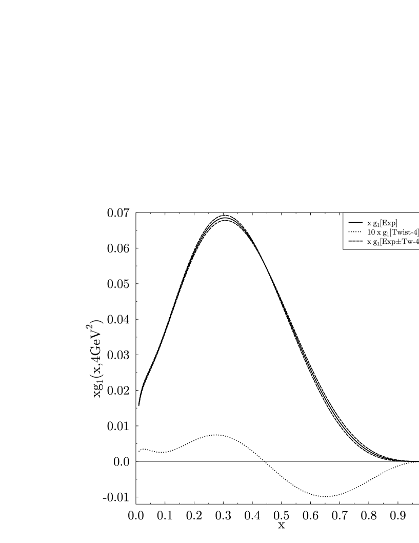
Figure 1: The experimental fit for $g_{1}(x,4\,{\rm GeV}^{2})$ (full line) [23]. The estimate for the twist-4 correction is given explicitly multiplied by a factor of $10$ (dotted line), showing a change in sign at $x\approx 0.43$. The correction was added and subtracted from the experimental values (dashed lines), so that the theoretical prediction of the twist-2 part of $g_{1}$ has to lie within this region ($\Lambda_{\overline{MS}}=200~{}{\rm MeV}$, $Q^{2}=4~{}{\rm GeV}$ and $N_{f}=4$).

Figure 2: The relative magnitude of the predicted twist-4 contribution to $g_{1}$ with respect to the experimental fit. $\Lambda_{\overline{MS}}=200~{}{\rm MeV}$, $Q^{2}=4~{}{\rm GeV}$ and $N_{f}=4$.

The ratio of the moments $M_{g_{1},n}^{tw4}$ of the twist-4 part of $g_{1}$ and $M_{g_{1},n}^{exp}$ of the experimental values for $g_{1}$ (containing all twist) reads

$$\frac{M_{g_{1},n}^{tw4}(Q^{2})}{M_{g_{1},n}^{exp}(Q^{2})} = \frac{C_{g_{1},n}^{(1)}\frac{\Lambda_{C}^{2}e^{-C}}{Q^{2}}+{\cal O}\left(\frac{a_{s}}{Q^{2}},\frac{1}{Q^{4}}\right)}{\sum_{k=0}^{m_{0}}B_{g_{1},n}^{(k)}a_{s}^{k}+C_{g_{1},n}^{(1)}\frac{\Lambda_{C}^{2}e^{-C}}{Q^{2}}+{\cal O}\left(\frac{a_{s}}{Q^{2}},\frac{1}{Q^{4}}\right)}$$ (16)

$$= C_{g_{1},n}^{(1)}\frac{\Lambda_{C}^{2}e^{-C}}{Q^{2}}+{\cal O}\left(\frac{a_{s}}{Q^{2}},\frac{1}{Q^{4}}\right)\,,$$

where we used $B_{g_{1},n}^{(0)}=1$. In this way $g_{1}^{tw4}(x,Q^{2})$ is expressed by a convolution of $g_{1}^{exp}(x,Q^{2})$:

$$g_{1}^{tw4}(x,Q^{2}) \!\!\!=\!\! \frac{\Lambda_{C}^{2}e^{-C}}{Q^{2}}\int_{x}^{1}\frac{dy}{y}\,g_{1}^{exp}\left(\frac{x}{y}\right)\,C_{g_{1}}^{{}^{\prime}(1)}(y)$$ (17)

$$\!\!\!=\!\! \frac{2C_{F}}{\beta_{0}}\frac{\Lambda_{C}^{2}e^{-C}}{Q^{2}}\bigg{\{}\int_{x}^{1}\frac{dy}{y}\,g_{1}^{exp}\left(\frac{x}{y}\right)(4+2y+4y^{2})-4\int_{x}^{1}\frac{dy}{y}\,g_{1}^{exp}\left(\frac{x}{y}\right)\frac{1}{(1-y)_{+}}$$

$$\hskip 62.59596pt+x\frac{d}{dx}g_{1}^{exp}(x)-4g_{1}^{exp}(x)\bigg{\}}$$

where $C_{g_{1}}^{{}^{\prime}(1)}(y)$ eq. (13) was inserted.

Using a fit to the available experimental data for $g_{1}$ [23], this expression indeed leads to very small twist-4 corrections to $g_{1}(x)$ (see fig. 1, 2). This result is not significant for the small $x$ region, where the large-$N_{F}$ limit is no longer justified.

From our general result for $g_{1}^{tw4}(x,Q^{2})$ eq. (17) we can also reproduce the renormalon prediction for the nonsinglet twist-4 matrix element [15]

$$\int_{0}^{1}dx\;g_{1}^{tw4}(x,Q^{2})\;=\;\pm\frac{4C_{F}}{3\beta_{0}}\frac{\Lambda_{C}^{2}e^{-C}}{Q^{2}}\int_{0}^{1}dx\;g_{1}^{exp}(x,Q^{2})\;\approx\;\pm\frac{0.017\,GeV^{2}}{Q^{2}}$$ (18)

in good agreement with our QCD sum rule result of $-\frac{0.0094\,GeV^{2}}{Q^{2}}$ [24]. Another renormalon estimate based on Padé approximants [25] gave a value of $\frac{\pm(0.04\pm 0.016)\,GeV^{2}}{Q^{2}}$. In the same way as we did in [17] we checked the cancellation of the above IR-renormalon contribution by the UV-renormalon contribution to the genuine twist-4 correction. Note that in addition to the twist-4 power correction to the Bjorken sum rule there exist twist-2 and twist-3 matrix elements, which are also power suppressed by $1/Q^{2}$ [26].

Finally we give an estimate for the error made in the determination of the nonsinglet twist-3 matrix element $d^{(2)}$ due to higher-twist corrections. The third moment of the nonsinglet structure function $g_{2}(x,Q^{2}):=g_{2}^{p}(x,Q^{2})-g_{2}^{n}(x,Q^{2})$ is given by

$$\int_{0}^{1}dx\,x^{2}g_{2}(x,Q^{2})\;=\;-\frac{1}{3}a^{(2)}+\frac{1}{3}d^{(2)}+{\cal O}\left(\frac{M^{2}}{Q^{2}}\right)$$ (19)

where $a^{(2)}$ is a pure twist-2 nonsinglet operator matrix element. So the twist-3 nonsinglet matrix element $d^{(2)}$ can be obtained by measuring $g_{2}(x,Q^{2})$ and $a^{(2)}$, which in turn is determined by the third moment of $g_{1}(x,Q^{2})$:

$$\int_{0}^{1}dx\,x^{2}g_{1}(x,Q^{2})\;=\;\frac{1}{2}a^{(2)}+{\cal O}\left(\frac{M^{2}}{Q^{2}}\right)$$ (20)

If one uses $a^{(2)}$ from the total measured $g_{1}(x,Q^{2})$, higher twist corrections to $g_{1}(x,Q^{2})$ are not distinguished from the twist-2 part. This leads to an error in the determination of $d^{(2)}$ of the order of the higher-twist correction to $g_{1}(x,Q^{2})$ [1]. Using our estimate for the nonsinglet twist-4 contribution to $g_{1}(x,Q^{2})$, we obtain the following uncertainty for $a^{(2)}$

$$2\int_{0}^{1}dx\;x^{2}g_{1}^{tw4}(x,Q^{2})\approx 0.0003\sim\Delta(a^{(2)})$$ (21)

The main contribution to the third moment of $g_{2}(x,Q^{2})$ comes from $a^{(2)}$, so that the above uncertainty leads to an error for $d^{(2)}$ of about $10\%$, which is substantially smaller than the present experimental error bars. We conclude that the mentioned procedures to determine $d^{(2)}$ and $\Delta G(x)$ from experimental data are not invalidated by higher-twist effect.

Acknowledgements. This work has been supported by BMBF, DFG (G.Hess Programm) and KBN grant 2 P03B 065 10. A.S. thanks also the MPI für Kernphysik in Heidelberg for support.

References

- [1] E143 Collaboration, K. Abe et al., Phys.Rev.Lett. 76 (1996), 587
- [2] M. Göckeler et al., Phys.Rev. D53 (1996), 2317
-
[3]
I.I. Balitsky, V.M. Braun, A.V. Kolesnichenko, Phys.Lett. B242
(1990), 245; Phys.Lett. 318 (E) (1993), 648
E. Stein, P. Górnicki, L. Mankiewicz, A. Schäfer, W. Greiner, Phys.Lett. B343 (1995), 369 - [4] R. Ball, S. Forte, G. Ridolfi, NLO determination of the singlet axial charge and the polarized gluon content of the nucleon. hep-ph/9510449
- [5] J. Lichtenstadt et al. (SMC collaboration), Contribution to the HERA-Workshop 1995/96: Future Physics at HERA, unpublished
-
[6]
A.H. Mueller, The QCD perturbation series.,
in “QCD - Twenty Years Later”, edited by P.M. Zerwas and H.A. Kastrup,
162, (World Scientific 1992)
V.I. Zakharov, Nucl.Phys. B385 (1992), 452
A.H. Mueller, Phys.Lett. B308 (1993), 355 -
[7]
M. Beneke, Nucl.Phys. B405 (1993), 424
M. Beneke, V.M. Braun, Nucl.Phys. B426 (1994), 301 -
[8]
D.J. Broadhurst,
Z.Phys. C58 (1993), 339
J.A. Gracey, Phys.Lett. B323 (1994), 141 - [9] D.J. Broadhurst and A.L. Kataev, Phys.Lett. B315 (1993), 179
- [10] C.N. Lovett-Turner, C.J. Maxwell, Nucl. Phys. B452 (1995), 188
-
[11]
D.J.Broadhurst and A.G.Grozin,
Phys.Rev. D 52 (1995), 4082
M. Neubert, Phys.Rev. D51 (1995), 5924 - [12] M. Beneke and V.M. Braun, Phys.Lett. B348 (1995), 513
- [13] P. Ball, M. Beneke and V.M. Braun, Nucl. Phys. B452 (1995), 563
-
[14]
Yu. L. Dokshitzer and N. G. Uraltsev,
Are IR renormalons a good probe for the strong interaction domain? hep-ph/9512407 (1995)
G. Grunberg, Phys.Lett. B372 (1996), 121 -
[15]
V. M. Braun,
QCD Renormalons and Higher Twist Effects. hep-ph/9505317 (1995)
M. Beneke and V.M. Braun, Nucl.Phys. B454 (1995), 253 - [16] Yu. L. Dokshitzer, G. Marchesini and B.R. Webber, Dispersive Approach to Power-Behaved Contributions in QCD Hard Processes, hep-ph/9512336 (1995), to appear in Nucl.Phys.
- [17] E. Stein, M. Meyer-Hermann, L. Mankiewicz, A. Schäfer, IR-renormalon Contribution to the Longitudinal Structure Function . hep-ph/9601356 (1996), to appear in Phys.Lett.B
- [18] M. Beneke, V.M. Braun, V.I. Zakharov, Phys.Rev.Lett. 73 (1994), 3058
- [19] T. Muta, Foundations of Quantum Chromodynamics, World Scientific 1987
- [20] N.S. Craigie, K. Hidaka, M. Jacob, F.M. Renard, Phys.Rep. 99 (1983), 69
- [21] S.A. Larin, J.A.M. Vermaseren, Phys.Lett. B259 (1991), 345
- [22] M. Dasgupta, B.R. Webber, Power Corrections and Renormalons in Deep Inelastic Structure Functions. hep-ph/9604388
- [23] T. Gehrmann, W.J. Stirling, Polarized Parton Distributions in the Nucleon. hep-ph/9512406 (1995), to appear in Phys.Rev.D
- [24] E. Stein, P. Gornicki, L. Mankiewicz, A. Schäfer, Phys.Lett. B353 (1995), 107
- [25] J. Ellis, E. Gardi, M. Karliner, M.A. Samuel, Phys.Lett. B366 (1996), 268
-
[26]
E.V. Shuryak, A.I. Vainshtein, Nucl.Phys. B201 (1982), 141
B. Ehrnsperger, L. Mankiewicz, A. Schäfer, Phys.Lett. B323 (1994), 439