Abstract

The present review gives a survey of recent developments and applications of the Nambu–Jona-Lasinio model with $N_{f}=2$ and $N_{f}=3$ quark flavors for the structure of baryons. The model is an effective chiral quark theory which incorporates the SU(N_f)${}_{L}\otimes$SU(N_f)${}_{R}\otimes$U(1)_V approximate symmetry of Quantum chromodynamics. The approach describes the spontaneous chiral symmetry breaking and dynamical quark mass generation. Mesons appear as quark-antiquark excitations and baryons arise as non-topological solitons with three valence quarks and a polarized Dirac sea. For the evaluation of the baryon properties the present review concentrates on the non-linear Nambu–Jona-Lasinio model with quark and Goldstone degrees of freedom which is identical to the Chiral quark soliton model obtained from the instanton liquid model of the QCD vacuum. In this non-linear model, a wide variety of observables of baryons of the octet and decuplet is considered. These include, in particular, electromagnetic, axial, pseudoscalar and pion nucleon form factors and the related static properties like magnetic moments, radii and coupling constants of the nucleon as well as the mass splittings and electromagnetic form factors of hyperons. Predictions are given for the strange form factors, the scalar form factor and the tensor charge of the nucleon.

“Though this be madness, yet there is method in it.”                                                                                               Shakespeare, Hamlet, II-2

——————————- E-mail: christov@hadron.tp2.ruhr-uni-bochum.de blotz@nuclear.physics.sunysb.edu kim@hadron.tp2.ruhr-uni-bochum.de pavelp@hadron.tp2.ruhr-uni-bochum.de watabe@hadron.tp2.ruhr-uni-bochum.de meissner@nuc003.psc.scarolina.edu earriola@ugr.es goeke@hadron.tp2.ruhr-uni-bochum.de

1.	Introduction	4
2.	SU(2) NJL model: vacuum sector and meson properties	8
2.1	Bosonization of the NJL model	8
2.2	Divergences and regularization	12
2.3	Spontaneously broken chiral symmetry and constituent quark mass	14
2.4	Mesonic properties	15
2.5	Fixing of the parameters in the vacuum sector	18
2.6	Restriction to Goldstone degrees of freedom: the chiral circle	19
2.7	Generalization to higher flavor groups and relation to the topological approach	21
3.	Nucleon as a non-topological soliton in the NJL model	23
3.1	Nucleon correlation function	24
3.2	“Classical” soliton	25
3.3	Baryon number of the soliton	27
3.4	Stationary hedgehog meson-field configuration	29
3.5	Selfconsistent soliton solution	32
3.6	Semiclassical quantization of the soliton	35
3.7	Nucleon matrix elements of quark current	41
4.	Nucleon properties in the SU(2) NJL model	47
4.1	Electromagnetic properties	47
4.2	$E2/M1$ ratio for the $\gamma N\rightarrow\Delta$ transition	53
4.3	Axial properties	55
4.4	Pion nucleon form factor	61
4.5	PCAC and the Goldberger-Treiman relation	63
4.6	Tensor charges	65
4.7	Electric polarizability of the nucleon	66
5.	SU(3)–Flavor NJL model	68
5.1	Extension of the NJL model to SU(3) flavors	68
5.2	Vacuum solutions and fixing of parameters	69
5.3	Restriction to Goldstone modes	71
5.4	Trivial embedding of SU(2) hedgehog soliton into SU(3)	72
5.5	Expansion in angular velocity	72
5.6	Strange mass terms of the collective lagrangian	75
5.7	Hyperon splittings in linear order - Sum rules	77
5.8	Hyperon splitting in second order - wave functions	78
5.9	Yabu-Ando diagonalization method	80
5.10	Results: mass splittings in the SU(3) NJL model	81
6.	Baryon properties in the SU(3) NJL model	84
6.1	Electromagnetic properties	84
6.2	Strange vector form factors of the nucleon and related observables	87
6.3	Scalar form factor and the sigma term $\pi N$	92
6.4	Axial charges of the nucleon	92
6.6	Gottfried sum rule	95
7.	Summary	97
	References	98

1 Introduction

The structure and the dynamics of hadrons are generally believed to be described by Quantum chromodynamics (QCD). A prominent feature of QCD is the asymptotic freedom which allows the processes at high energies to be described perturbatively in terms of these degrees of freedom. However, at energies comparable to the low-lying hadron masses QCD shows non-perturbative phenomena such as confinement of quarks and gluons and the spontaneous breakdown of chiral symmetry. It makes the description in terms of quarks and gluons enormously complicated and the only direct source of information from QCD is the lattice Monte Carlo simulations. In this situation it is natural to invoke effective models of the strong interaction which incorporate the relevant degrees of freedom in the low energy regime. Those are all related to chiral symmetry and its dynamical breaking. In fact, the spontaneous breakdown of the chiral symmetry has been phenomenologically recognized to be an essential feature of the strong interaction long before the advent of QCD. One has by now accumulated a large number of empirical facts and, following from this, somewhat generally accepted features of low energy hadronic dynamics, which have to be respected by effective models:

• The existence of light pseudoscalar mesons (pions) and the fact that there is no degenerate partner of the nucleon with negative parity suggests that the pions are Goldstone bosons associated with the dynamical breaking of SU(2)${}_{L}\otimes$SU(2)_R chiral flavor symmetry down to SU(2)_V. This picture can be extended to SU(3), although obviously the larger masses of kaons and $\eta$ indicate that the explicit chiral symmetry breaking is larger in this case.

• The relatively large mass of $\eta^{\prime}$ suggests that the flavor $U_{A}$(1)-current is not conserved even in chiral limit.

• The hadron mass differences in the SU(3)-flavor multiplets appear as being governed by a linear breaking of the SU(3)_V-symmetry in a rather simple fashion and follow phenomenologically the Gell-Mann-Okubo mass formula.

• The masses of the low lying mesons and baryons, apart from the Goldstone bosons, are quite well described in terms of the constituent quark model whose basic ingredients are massive constituent up and down ($M_{u,d}~{}\approx 350$ MeV) and strange ($M_{s}~{}\approx 500$ MeV) quarks.

Actually the above empirical facts can be understood from the viewpoint of QCD. Its lagrangian is given by

$${\cal L}_{\rm QCD}=\bar{\Psi}(i\gamma^{\mu}\partial_{\mu}+g\gamma^{\mu}A_{\mu}-\hat{m})\Psi-{1\over 2}{\rm Sp}F_{\mu\nu}F^{\mu\nu}\,.$$ (1)

Here $\Psi$ comprises a quark field with $N_{c}=3$ colors and $N_{f}=6$ flavors, and $A_{\mu}$ and $F_{\mu\nu}$ are the corresponding SU(3)-color gauge field and field strength tensor, respectively.

The current quark masses are represented in (1) by the matrix $\hat{m}={\rm diag}(m_{u},m_{d},m_{s},m_{c},m_{b},m_{t})$. Since up-, down- and strange current quark masses are much smaller than those of other quarks, there is a natural separation between “light quark physics”, relevant for energies $\sim~{}1$ GeV, and “heavy quark physics” for higher energies. Thus for systems composed of up-, down- and strange quarks one can ignore the heavy quarks and work with $N_{f}=2$ or 3. Accordingly it is physically reasonable to consider the limit of vanishing (light) current quark masses and if needed the current quark masses can be treated as perturbations. This limit corresponds to exact chiral symmetry. The latter is broken spontaneously which results in a non-zero chiral condensate $\langle 0|\bar{\Psi}\Psi|0\rangle$. The breakdown of chiral symmetry leads to the appearance of Goldstone bosons and to a dynamical generation of a constituent quark mass of a few hundred MeV. Although for many observables one can probably neglect $m_{u}$ and $m_{d}$, the finite value of $m_{s}~{}\approx~{}175$ MeV is too large to be ignored. In particular, the relatively large current strange mass $m_{s}$ is responsible for the baryon mass splitting summarized in the Gell-Mann-Okubo mass formula.

The number of colors $N_{c}$ plays a special role in QCD. The inverse number of colors $1/N_{c}$ can be considered (’t Hooft, 1974) as a small parameter of QCD. Although in the real world $N_{c}=3$, the $1/N_{c}$ expansion is a very useful tool to analyze non-perturbative phenomena in the QCD. We will use this technique also in the effective theory considered below. In fact, concepts like that of constituent quarks and the idea of describing baryons as chiral solitons with a polarized Dirac sea emerge naturally from the large $N_{c}$ limit of QCD and have proven to be phenomenologically quit useful.

In this report we shall concentrate on theory and applications of an effective model, which on one hand is formulated in terms of quarks interacting via a simple and tractable quark-antiquark interaction, and on the other hand fulfills basically the above mentioned phenomenological demands, in particular the dynamical chiral symmetry breaking and the explicit symmetry breaking due to current quark masses. The model has first been proposed by Nambu and Jona-Lasinio (1961a,b) in a different context. It has become quite popular and successful in a form where the fermion fields are re-interpreted as quark fields. In the meson sector it has already been the subject of several review articles (Vogl and Weise, 1991, Klevansky, 1992, Hatsuda and Kunihiro, 1994). In the baryon sector the most interesting aspect is the applications to physical observables of nucleon and hyperons and this is the subject of the present report. Previous reviews cover only partially these topics (Meissner et al., 1993, Alkofer et al., 1995). The Nambu – Jona-Lasinio (NJL) model provides an excellent account of the today’s experimental data if both the collective quantization and the perturbative expansion in $m_{s}$ are performed properly. The model describes the physics in a way quite different from the other well known baryonic effective model, i.e. the Skyrme model (Skyrme 1961, 1962). In the Skyrme-approach (Adkins et al., 1993, Holzwarth and Schwesinger, 1986, Zahed and Brown, 1986) one does not have quarks but meson fields and the baryons are described as topological solitons. In fact, the NJL model contains this physical picture as a limiting case, though being a genuine non-topological model. The relationship between these two approaches will also be a subject of discussion of our review.

The NJL model in its simplest SU($N_{f}=2$)-form is given by

$${\cal L}=\bar{\Psi}(i\gamma^{\mu}\partial_{\mu}-m_{0})\Psi+{G\over 2}[(\bar{\Psi}\Psi)^{2}+(\bar{\Psi}i\gamma_{5}\vec{\tau}\Psi)^{2}]\,.$$ (2)

Here $\Psi$ are quarks fields, which are flavor doublets with $N_{c}=3$ colors, and $m_{0}$ is the average up and down quark current mass. The corresponding semibosonized lagrangian is

$${\cal L}^{\prime}={\bar{\Psi}}(i\hbox to0.0pt{\hbox to5.30904pt{\hfil/\hfil}\hss}\partial-\sigma-i\vec{\pi}\cdot\vec{\tau}\,\gamma_{5})\Psi-{1\over 2G}(\sigma^{2}+\vec{\pi}^{2})+{m_{0}\over G}\sigma\,,$$ (3)

where $\sigma$ and $\vec{\pi}$ are auxiliary meson fields. The model is not renormalizable and lacks confinement. Although these features were for many years a reason to ignore the NJL model, nowadays the view is different. For an effective model in the low energy regime, the problem of non-renormalizability can be avoided if one has a reasonable means to fix a suitable ultraviolet cut-off. The lack of confinement provides in NJL model unphysical $\bar{\Psi}\Psi$-thresholds. However, there are strong arguments that the basic properties of light hadrons can be reproduced without invoking confinement and one of them is the recent lattice QCD results for the correlation functions of hadronic currents in the cooled vacuum (Chu et al., 1994). This point of view will be also supported by the results reviewed in the present paper.

In the NJL model, baryons appear as large $N_{c}$ solutions consisting of valence quarks bound to the Dirac sea via classical (mean-field) meson fields in accordance with the arguments of Witten (1979). This physical picture was proposed by Kahana and Ripka (1984), and by Diakonov et al. (1986). However, the mean-field solutions exist only if the classical meson fields are subjected to the condition of the chiral circle

$$\sigma^{2}+\vec{\pi}^{2}=M^{2}\,,$$ (4)

where $M$ is the dynamically generated constituent quark mass. Under this constraint the NJL lagrangian (3) reduces to an effective lagrangian

$${\cal L}^{\prime}=\bar{\Psi}(i\gamma^{\mu}\partial_{\mu}-m_{0}-MU^{\gamma_{5}})\Psi\,,$$ (5)

in which the quarks interact only with Goldstone fields and the SU(2) matrix $U$ corresponds to a non-linear representation of the pion field $MU^{\gamma_{5}}=\sigma+i\gamma_{5}\vec{\pi}\vec{\tau}$. For SU(3) the chiral field configuration $U$ also encompasses kaon and eta fields. In the actual calculations $U$ will be determined selfconsistently by minimizing the effective action which corresponds to ${\cal L}^{\prime}$ (5). The model with constraint (4) is usually referred to as the non-linear NJL model or, when applied to baryons, the Chiral quark soliton model.

The assumption of the chiral circle (non-linear pion field configuration) is not an ad hoc device to allow for solitonic solutions of NJL. Physically, it is a means of separating low-energy mesonic degrees of freedom (Goldstone bosons) from heavier ones (sigma meson) and to “freeze” the latter. The physics, which apparently goes beyond the scope of the NJL model, can be understood in the framework of the underlying theory, the low-energy QCD.

There are various attempts (McKay and Munczek, 1985, Cahill and Roberts, 1985, Diakonov and Petrov, 1986, Ball, 1989, Schaden et al., 1990) to relate the NJL model to some low-energy limit of QCD. Further, arguments to illuminate the chiral structure of the NJL model are given by Ebert and Volkov (1983), Volkov (1984), Dhar and Wadia (1984) and Ebert and Reinhardt (1986). The relationship to the chiral perturbation theory (Gasser and Leutwyler, 1982) is studied by Hansson et al. (1990), Bernard and Meissner (1991), Ruiz Arriola (1991), Schüren et al. (1992) and Bijnens et al. (1993). In fact, the physics behind the present model can be well understood in the framework of the instanton liquid model of QCD (Shuryak 1982, 1983, Diakonov and Petrov, 1984, 1986) which is also supported by recent lattice QCD calculations (Chu et al., 1994). The assumption that the non-perturbative ground state of QCD is governed by a dilute liquid of interacting instantons and anti-instantons allows to obtain in large $N_{c}$ limit an effective low-energy theory (Diakonov and Petrov, 1986) which can be used to justify the NJL lagrangian on the chiral circle, i.e. eq. (5). In fact, by assuming the instanton model of the QCD vacuum, Diakonov and Petrov (1984, 1986) derived an effective low-energy QCD lagrangian in terms of a ’t Hooft-like $2N_{f}$-fermion interaction. The crucial quantity in the instanton vacuum is the ratio $\bar{\rho}/\bar{R}$ of the average size $\bar{\rho}$ of instantons to the average distance $\bar{R}$ between them. Both the phenomenological analysis (Shuryak 1982, 1983) and the variational estimates (Diakonov and Petrov, 1984) suggested a relatively small value $\bar{\rho}/\overline{R}\approx 1/3$ which has been confirmed by the lattice calculations (Chu et al., 1994). Thus, besides the inverse number of colors $1/N_{c}$ this small ratio plays also an important role of a small parameter in the theory. If one places light quarks in the instanton vacuum, one observes that chiral symmetry is dynamically broken due to the delocalization of the would-be fermion zero modes related to the individual instantons. Spontaneous chiral symmetry breaking manifests itself in a non-zero chiral condensate $\langle 0|\bar{\Psi}\Psi|0\rangle$, massless Goldstone bosons, and in a momentum dependent dynamical quark mass $M(k)$ with $M(0)\approx 350$ MeV and $M(k)$ vanishing for momenta $k\gg 1/\bar{\rho}$. Due to the instanton-induced ’t Hooft-like interaction the $\eta^{\prime}$ is not a Goldstone boson, so that the $U_{A}(1)$ problem is properly solved. The momentum dependence of $M(k)$ provides a natural cut-off $1/\bar{\rho}$ which makes the resulting theory finite. It is important that the dynamical quark mass is parametrically small $M\bar{\rho}=O(\bar{\rho}^{2}/\bar{R}^{2})\ll 1$ compared to the cutoff $1/\bar{\rho}$. As a final result, due to the diluteness parameter $\bar{\rho}/\overline{R}$ in this instanton model of QCD vacuum, at low momenta $k<1/\bar{\rho}$ and large $N_{c}$ the QCD is reduced to an effective quark meson theory with a lagrangian which includes only constituent quarks of mass $M(k)$ interacting with Goldstone pion fields. If both quark and pion momenta are smaller than $1/\bar{\rho}$ the dynamical mass $M(k)$ can be approximated by $M=M(0)$. In this approximation one reproduces the semibosonized NJL lagrangian (5). Since the inverse size of nucleons corresponds to $\sim 300$ MeV this can be considered as “much” less than the cutoff $1/\bar{\rho}$ and the effective lagrangian (5) can be also applied to describe baryons. Hence a systematic treatment of the nucleons and hyperons involves only quarks and Goldstone bosons, and the implementation of the chiral circle in (3) is justified. It should be noted that the only relevant degrees of freedom are pions and quarks and excitations connected with other degrees of freedom like vector mesons have $k\sim 1/\bar{\rho}$ and do not contribute essentially to the dynamics at momenta $k\ll 1/\bar{\rho}$. Following this logic one realizes that for a proper description of the baryon ground-state properties the only relevant degrees of freedom are those of quarks and pions, and heavier meson degrees of freedom like scalar and vector mesons are not important.

The present paper concentrates on the results for the baryon properties in the non-linear NJL model. The paper reviews applications in flavor SU(2) and SU(3) versions to electromagnetic, axial, scalar and strange vector form factors and the related static properties like magnetic moments, radii and coupling constants of the nucleon, and to the mass splittings and electromagnetic properties of the hyperons of the octet and decuplet. Calculations of the spin properties are discussed in connection with the “spin crisis”. Predictions are reviewed also for nucleon strange form factors and tensor charges. For all observables, the calculations reported are performed with one and the same set of parameter values. These values are fixed in the meson sector by fitting the physical values of the pion mass and the pion decay constant, and additionally to the kaon mass in the case of SU(3). The only parameter, which is free, is the constituent mass $M$. However, as we will show for the constituent mass of about $M=420$ MeV the model is rather successful in describing the baryon properties. Actually, the comparison of the model results with the experimental data of the nucleon and also of the hyperons in the octet and decuplet shows that the NJL model on the chiral circle indeed is able to reproduce most of the data within 15 %. This includes critical observables like the axial vector coupling constant, $g_{A}$, and the magnetic moments of proton and neutron. Only a few observables are less successfully described (within 30 %) as e.g. the neutron electric form factor and the corresponding charge radius.

Since the present theory yields a rather good agreement with the experimental data one can use the model picture to obtain some insight into the low-energy structure of the nucleon and the other octet and decuplet baryons. The basic mechanism is obviously the interaction of quarks with pseudoscalar Goldstone bosons, the latter being themselves quark-antiquark excitations of the spontaneously broken chiral vacuum. Heavier mesons like scalar mesons or vector mesons are apparently not needed in this scenario. In addition, the confining forces seem also not to be much relevant in describing the ground-state properties of low mass mesons and baryons. Hence, the only important mechanism seems to be chiral symmetry breaking. The calculations support the physical picture of baryons as non-topological solitons of $N_{c}=3$ valence quarks bound to a polarized Dirac sea via classical (mean-field) meson fields and being well separated from the negative Dirac continuum. The polarized Dirac sea phenomenologically corresponds to a meson cloud. Most of the observables receive about 30 % contributions from the Dirac sea quarks. This valence picture of the baryon in the present model differs from the one of the topological solitons favored in the Skyrme model. In principle, the NJL model can be reduced to a topological approach similar to the Skyrme model by an expansion of the effective action in terms of gradients of the meson fields (gradient expansion). This expansion does only converge if the valence level is close to the negative Dirac continuum. This, however, requires in the NJL model unphysically large values of the constituent mass for which the baryon properties are not reproduced. Hence, within the NJL model there is no way to recover Skyrme type models.

2 SU(2) NJL model: vacuum sector and meson properties

In this chapter we deal with the Nambu – Jona Lasinio model with two lightest quark flavors. To begin with, we study the NJL lagrangian and its symmetries. Using the functional integral approach we bosonize the theory and solve the effective bosonized theory in the mean-field approximation which corresponds to the leading order of the expansion in inverse number of quark colors. In the functional integral approach the mean-field solution naturally appears as a saddle point of the bosonized action. We analyze the structure of the ultraviolet divergences of the model and introduce the regularization scheme. We show that in the mean-field treatment of the model chiral symmetry is spontaneously broken, which leads to a generation of the constituent quark mass. An important consequence of the spontaneous breakdown of chiral symmetry is the appearance of light Goldstone mesons (pions). We discuss shortly the description of mesons in the model and sketch the derivation of the meson propagators, masses and of the meson decay constant needed to fix the model parameters.

2.1 Bosonization of the NJL model

NJL lagrangian and its symmetries. The NJL lagrangian contains a local four-fermion interaction. In the simplest SU(2) version it includes only scalar and pseudoscalar couplings:

$${\cal L}=\bar{\Psi}(x)\Bigl{[}i\hbox to0.0pt{\hbox to5.30904pt{\hfil/\hfil}\hss}\partial-{\hat{m}}\Bigr{]}\Psi(x)+{G\over 2}\Bigl{[}\Bigl{(}\bar{\Psi}(x)\Psi(x)\Bigr{)}^{2}+\Bigl{(}\bar{\Psi}(x)i\gamma_{5}{\vec{\tau}}\Psi(x)\Bigr{)}^{2}\Bigr{]}$$ (6)

where one recognizes the free and the interaction parts

$${\cal L}_{free}=\bar{\Psi}(x)\Bigl{[}i\hbox to0.0pt{\hbox to5.30904pt{\hfil/\hfil}\hss}\partial-{\hat{m}}\Bigr{]}\Psi(x)\,,$$

$${\cal L}_{int}={G\over 2}\Bigl{[}\Bigl{(}\bar{\Psi}(x)\Psi(x)\Bigr{)}^{2}+\Bigl{(}\bar{\Psi}(x)i\gamma_{5}{\vec{\tau}}\Psi(x)\Bigr{)}^{2}\Bigr{]}$$ (7)

respectively. Here $\Psi(x)$ denotes a quark field with $u$ and $d$ flavors and $N_{c}$ colors. The matrices $\tau^{a}$ $(a=1,2,3)$ are usual Pauli matrices. The $\hat{m}$ represents the current quark mass matrix given by

$${\hat{m}}=\left(\matrix{m_{u}&0\cr 0&m_{d}}\right)=m_{0}{\bf 1}+\tau_{3}m_{3}\,.$$ (8)

It is useful to divide it in the average mass $m_{0}$ and in the isospin mass difference $m_{3}$ defined as

$$m_{0}={1\over 2}(m_{u}+m_{d}),\qquad m_{3}={m_{u}-m_{d}\over 2}\,.$$ (9)

In (6) $G$ is the coupling constant of the four fermion interaction.

Lagrangian (6) possesses a number of symmetries which we also have in QCD. In particular, it is symmetric under the global $U(1)$ transformation

$$\Psi(x)\rightarrow\Psi^{\prime}(x)=\exp(i\delta)\Psi(x)\,.$$ (10)

If one neglects the quark isospin mass difference $m_{3}$ and considers $m_{u}=m_{d}=m_{0}$, which corresponds to exact isospin symmetry, lagrangian (6) is also invariant under the transformation

$$\Psi(x)\to\Psi^{\prime}(x)=\exp(i\vec{\tau}\cdot\vec{\rho})\Psi(x)\,.$$ (11)

If we additionally neglect the current mass $m_{0}$, it becomes invariant under global chiral transformations:

$$\Psi(x)\to\Psi^{\prime}(x)=\exp(i\gamma_{5}\vec{\tau}\cdot\vec{\kappa})\Psi(x)\,.$$ (12)

Thus, in chiral limit $m_{u}=m_{d}=0$, the NJL lagrangian has an $SU_{L}(2)\otimes SU_{R}(2)\otimes U_{V}(1)$ symmetry. Therefore, many well-known results obtained within the current algebra can be reproduced in the NJL model. Later we will show that chiral symmetry is spontaneously broken which leads to such fundamental consequences as the appearance of Goldstone bosons (pions) and to the generation of the dynamical quark mass.

The above transformations correspond to the following Noether currents

$$B_{\mu}(x)=\bar{\Psi}(x)\gamma_{\mu}\Psi(x)\qquad\hskip 24.18501pt{\rm(baryon\,current)}\,,$$ (13)

$$V_{\mu}^{a}(x)=\bar{\Psi}(x)\gamma_{\mu}{\tau^{a}\over 2}\Psi(x)\qquad\hskip 11.38092pt{\rm(vector\,current)}\,,$$ (14)

$$A_{\mu}^{a}(x)=\bar{\Psi}(x)\gamma_{\mu}\gamma_{5}{\tau^{a}\over 2}\Psi(x)\qquad\hskip 8.5359pt{\rm(axial\,current)}\,,$$ (15)

whose divergences are given by

$$\partial^{\mu}B_{\mu}=0\,,$$ (16)

$$\partial^{\mu}V_{\mu}^{a}=i\bar{\Psi}[{\hat{m}},{\tau^{a}\over 2}]\Psi\,,$$ (17)

$$\qquad\partial^{\mu}A_{\mu}^{a}=i\bar{\Psi}\gamma_{5}\{{\hat{m}},{\tau^{a}\over 2}\}\Psi\,.$$ (18)

The baryon current and the third component of the vector isotopic current $V_{\mu}^{3}$ are conserved for any values of the quark masses. For the conservation of $V_{\mu}^{1}$, $V_{\mu}^{2}$ we need equal quark masses $m_{u}=m_{d}$, whereas the axial current $A_{\mu}^{a}$ is conserved only in chiral limit $m_{u}=m_{d}=0$, so that the last equation (18) expresses the partial conservation of the axial current (PCAC).

Below for simplicity we work with the NJL model in the approximation $m_{u}=m_{d}=m_{0}$. However, most of our formalism can be easily generalized to the case $m_{u}\neq m_{d}$ at least in the linear approximation in small quark masses.

The NJL lagrangian is assumed to mimic the low energy effective theory of QCD with gluon degrees of freedom integrated out. However the quark fields carry a color index that runs from $1$ to $N_{c}$ ($N_{c}=3$ in the real world). Instead of the $SU(N_{c})$ local gauge invariance of QCD, in the NJL lagrangian, we have only the global $SU(N_{c})$ invariance. Although the color degrees of freedom enter the NJL lagrangian in a rather trivial way, their role will be very important for the justification of the mean-field approximation to the NJL model. Later we shall show that the mean-field approach becomes asymptotically exact in the limit of large number of quark colors $N_{c}$.

Auxiliary boson fields. The NJL lagrangian (6) contains only quark degrees of freedom. On the other hand, the light mesons which we are going to describe by using this effective lagrangian are pions. Therefore, it is desirable to find an equivalent formulation of the theory that involves meson fields and not only quarks. Another reason why we need the bosonization is that we are going to solve the model by using the mean field approximation. In terms of the functional integral approach the mean field solution corresponds to the saddle-point approximation. The saddle-point solution can be obtained only in terms of boson fields so that the bosonization of the NJL lagrangian is a natural step towards the mean-field solution of this model.

Historically, the bosonization has first been formulated in solid state physics where it is known as Hubbard-Stratononovich transformation. In the present theory it has been first applied by Eguchi (1976), Kikkawa (1976) and Kleinert (1976).

For simplicity we describe the bosonization of NJL on the level of the partition function

$$Z=\int{\cal D}\Psi{\cal D}\bar{\Psi}\mbox{e}^{i\int{d}^{4}x{\cal L}(x)}$$ (19)

keeping in mind that the generalization to other quantities is straightforward.

Under proper normalization of the integration measure one can write the following identity

$$1=\int{\cal D}\sigma{\cal D}\vec{\pi}\exp\biggl{\{}-i\int d^{4}x{1\over 2G}\left[\left(\sigma+G\left(\bar{\Psi}\Psi-{m_{0}\over G}\right)\right)^{2}+\left(\vec{\pi}+G\bar{\Psi}i\vec{\tau}\,\gamma_{5}\Psi\right)^{2}\right]\biggr{\}}$$ (20)

with a gaussian path integral over auxiliary boson fields $\sigma$ and $\vec{\pi}$ on the rhs. Inserting this identity into the partition function $Z$ we obtain:

$$Z=\int{\cal D}\bar{\Psi}{\cal D}\Psi{\cal D}\sigma{\cal D}\vec{\pi}\mbox{e}^{i\int\mbox{d}^{4}x{\cal L}^{\prime}(x)}\,,$$ (21)

where the path integral runs over both the quark and auxiliary meson fields. The corresponding semibosonized lagrangian is

$${\cal L}^{\prime}={\bar{\Psi}}(i\hbox to0.0pt{\hbox to5.30904pt{\hfil/\hfil}\hss}\partial-\sigma-i\vec{\pi}\cdot\vec{\tau}\,\gamma_{5})\Psi-{1\over 2G}(\sigma^{2}+\vec{\pi}^{2})+{m_{0}\over G}\sigma\,.$$ (22)

One should keep in mind that on this stage the introduced auxiliary fields $\sigma$ and $\vec{\pi}$ are non-dynamical fields and no kinetic term ${1\over 2}\left[\partial_{\mu}\sigma\partial^{\mu}\sigma+\partial_{\mu}\vec{\pi}\partial^{\mu}\vec{\pi}\right]$ appears in lagrangian (22). However, after integrating out the quarks in (21), i.e. after including the quark loop effects, the fields will be “dressed” and can describe the physical mesons. It should be stressed that since the bosonization procedure is exact, the semibosonized lagrangian ${\cal L^{\prime}}$ has the same symmetries as the initial lagrangian (6). Note that the meson fields $\sigma$, $\vec{\pi}$ transform under the chiral rotation (12) as follows

$$(\sigma+i\vec{\pi}\cdot\vec{\tau})\to(\sigma^{\prime}+i\vec{\pi}{}^{\prime}\cdot\vec{\tau})=\exp(-i\vec{\tau}\cdot\vec{\kappa})(\sigma+i\vec{\pi}\cdot\vec{\tau})\exp(-i\vec{\tau}\cdot\vec{\kappa})\,.$$ (23)

Diagrammatically, the described bosonization procedure corresponds to rearrangement and resummation of the graphs of the 4-fermion point interaction into quark-meson vertices of the Yukawa type by introducing collective scalar-isoscalar ($\sigma$) and pseudoscalar-isovector ($\vec{\pi}$) auxiliary boson fields, both carrying the quantum numbers of the composite operators $({\bar{\Psi}}\Psi)$ and $({\bar{\Psi}}i\vec{\tau}\gamma_{5}\Psi)$ but not color. The idea has a long history and traces back to the sixties (see for instance (Coleman, 1985) and references therein).

Effective action. Now instead of the four-fermion interaction we have a theory of quarks interacting with boson fields. Next we notice that the integral over quark fields in eq. (21) is gaussian and can be done exactly, which leads to a determinant of the Dirac operator

$$\int{\cal D}\bar{\Psi}{\cal D}\Psi\exp\left[i\int\mbox{d}^{4}x{\bar{\Psi}}(i\hbox to0.0pt{\hbox to5.30904pt{\hfil/\hfil}\hss}\partial-\sigma-i\vec{\pi}\cdot\vec{\tau}\,\gamma_{5})\Psi\right] = \mbox{Det}^{N_{c}}(i\hbox to0.0pt{\hbox to5.30904pt{\hfil/\hfil}\hss}\partial-\sigma-i\vec{\pi}\cdot\vec{\tau}\,\gamma_{5})$$ (24)

$$= \exp\left[N_{c}\mbox{Tr}\,\log(i\hbox to0.0pt{\hbox to5.30904pt{\hfil/\hfil}\hss}\partial-\sigma-i\vec{\pi}\cdot\vec{\tau}\,\gamma_{5})\right]\,.$$

Here the power of $N_{c}$ appeared due to $N_{c}$ colors of the quark fields.

The Dirac operator can be rewritten in the form

$$i\hbox to0.0pt{\hbox to5.30904pt{\hfil/\hfil}\hss}\partial-\sigma-i\vec{\pi}\cdot\vec{\tau}\,\gamma_{5}=\gamma^{0}[i\partial_{t}-h(\sigma,\vec{\pi})]\,.$$ (25)

where $h(\sigma,\vec{\pi})$ is the one-particle Dirac hamiltonian

$$h(\sigma,\vec{\pi})=-i\gamma^{0}\gamma^{k}\nabla_{k}+\gamma^{0}(\sigma+i\vec{\pi}\cdot\vec{\tau}\gamma_{5})\,.$$ (26)

Below we prefer to work with the euclidean time $\tau$ and perform the Wick rotation

$$\tau=it\,.$$ (27)

In the euclidean case the following change should be done in (24)

$$\mbox{Det}(i\hbox to0.0pt{\hbox to5.30904pt{\hfil/\hfil}\hss}\partial-\sigma-i\vec{\pi}\cdot\vec{\tau}\,\gamma_{5})=\mbox{Det}[i\partial_{t}-h(\sigma,\vec{\pi})]\to\mbox{Det}[\partial_{\tau}+h(\sigma,\vec{\pi})]\,.$$ (28)

Integrating out the quarks as it is done in (24) we arrive at the following completely bosonized euclidean effective action

$$S(\sigma,\vec{\pi})=-N_{c}\mbox{Tr}\,\log\,D(\sigma,\vec{\pi})+{1\over 2G}\int\mbox{d}^{4}x(\sigma^{2}+\vec{\pi}^{2})-{m_{0}\over G}\int d^{4}x\sigma\,.$$ (29)

Here we use the notation

$$D(\sigma,\vec{\pi})=\partial_{\tau}+h(\sigma,\vec{\pi})\,.$$ (30)

Large $N_{c}$ and mean-field approximation. In terms of the effective action (29) the partition function of the model is given by equation

$$Z=\int{\cal D}\sigma{\cal D}\vec{\pi}\mbox{e}^{-S(\sigma,\vec{\pi})}\,.$$ (31)

All our formulas, which have been derived so far, are exact. However, in order to evaluate the functional integral (31) we need some approximation. Note that the fermion determinant contribution to the effective action (29) has a prefactor of $N_{c}$. For a consistent large $N_{c}$ treatment of the effective action (29) we take the coupling constant of the NJL model to be of order

$$G=O(N_{c}^{-1})\,.$$ (32)

Then all terms in (29) will be of order $O(N_{c})$ and in large $N_{c}$ limit the functional integral (31) can be evaluated in the saddle-point approximation. The stationary meson configuration $\sigma_{c},\vec{\pi}_{c}$ minimizing the effective action $S(\sigma,\vec{\pi})$ can be found by solving the saddle point equations

$${\delta S(\sigma,\vec{\pi})\over\delta\sigma}\Bigr{|}_{\sigma=\sigma_{c}\atop\pi=\pi_{c}}=0\,,\qquad{\delta S(\sigma,\vec{\pi})\over\delta\vec{\pi}}\Bigr{|}_{\sigma=\sigma_{c}\atop\pi=\pi_{c}}=0\,.$$ (33)

Thus, in the leading order of the $1/N_{c}$ expansion the functional integral (31) is simply given by the value of the integrand at the saddle point. One can show that this approximation is nothing else but the Hartree mean-field approximation in the original $4$-fermion version, which has been used repeatedly (Bernard et al., 1984, Bernard, 1986, Ferstl et al., 1986, Bernard et al., 1987, Providencia et al., 1987, Bernard et al., 1988, Klimt et al., 1990) and has been reviewed by Vogl and Weise (1991) and Klevansky (1992).

2.2 Divergences and regularization

Like the Fermi theory of weak interaction the Nambu–Jona-Lasinio model is non-renormalizable, because the coupling constant of the 4-fermion interaction $G$ has the dimension $[G]=mass^{-2}$. This means that in each increasing order in $G$ new graphs with a higher degree of ultraviolet divergence appear. In order to get a well defined theory it is therefore necessary to specify how the infinities of the model have to be treated.

One faces the ultraviolet divergences in the effective action (29) already in the leading order in $N_{c}$ which are due to the Dirac determinant $\mbox{Det}\,D(\sigma,\vec{\pi})$. It is convenient to consider separately the divergences of the real part

$${\rm Re}\,\mbox{Tr}\,\log\,D={1\over 2}\,\mbox{Tr}\,\log\,(D^{{\dagger}}D)\,,$$ (34)

as well as of the imaginary part

$${\rm Im}\,\mbox{Tr}\,\log\,D={1\over 2i}\,\mbox{Tr}\,\log\,(D/D^{{\dagger}})\,.$$ (35)

UV divergences. Let us start from the real part of the effective action (34). The functional determinant $\mbox{Det}(D^{{\dagger}}D)$ is a complicated non-local functional of fields $\sigma,\vec{\pi}$ and the simplest way to study its divergences is to consider the case of slowly changing fields $\sigma,\vec{\pi}$ and to expand this functional determinant in a series of integrals of local polynomials in derivatives of fields $\sigma,\vec{\pi}$ (Aitchison and Fraser, 1984, 1985a, 1985b). It should be noted that in the case of the proper-time regularized effective action (see next subsection eq. (41)) for a systematic expansion it is more convenient to use the heat kernel method (Kleinert, 1976, Nepomechie, 1985, Ebert and Reinhardt, 1986). However, the structure of divergent terms can be determined by a simple dimensional analysis without explicit calculations. Since the effective action is dimensionless and the divergent terms should contain a positive power or the logarithm of the cutoff, the local integrals of the fields and their derivatives in the divergent terms should have a dimension of $mass^{m}$ where $m\geq 0$. Combining this dimensional argumentation with the chiral symmetry it is easy to see that the divergent terms are of the form

$${\rm Re}\,\mbox{Tr}\,\log\,\,D = c_{1}\int d^{4}x(\sigma^{2}+\vec{\pi}^{2})+c_{2}\int d^{4}x(\sigma^{2}+\vec{\pi}^{2})^{2}$$ (36)

$$+ c_{3}\int d^{4}x[(\partial^{\mu}\sigma)(\partial_{\mu}\sigma)+(\partial^{\mu}\vec{\pi})(\partial_{\mu}\vec{\pi})]+{\tilde{S}}(\sigma,\vec{\pi})\,.$$

Here $c_{1}$, $c_{2}$, $c_{3}$ are some divergent coefficients and ${\tilde{S}}(\sigma,\vec{\pi})$ stands for the ultraviolet finite part. Apparently, in order to examine the particular divergent structure of coefficients $c_{i}$ one should perform explicitly a gradient expansion of the real part of the effective action (34). Note that among the divergent terms there appeared the kinetic term for meson fields $\sigma,\vec{\pi}$. Later we will introduce a regularization so that this kinetic term will be finite but non-vanishing. The presence of this kinetic term means that the mesonic fields, which initially have been introduced as auxiliary unphysical fields, become dynamical fields after taking into account the quark loop effects.

Imaginary part of the effective action. In the case of the $SU(2)$ flavor group the imaginary part of the effective action vanishes. It is connected to the fact that operators $D(\sigma,\vec{\pi})$ and $D^{\ast}(\sigma,\vec{\pi})$ (the asterisk stands for usual complex, not hermitian, conjugation) are unitary equivalent in the $SU(2)$ case

$$D^{\ast}(\sigma,\vec{\pi})=V\tau^{2}D(\sigma,\vec{\pi})(V\tau^{2})^{\dagger}\,.$$ (37)

Here $V$ is some unitary spin matrix defined by

$$\gamma_{\mu}^{\ast}=V\gamma_{\mu}V^{-1}\qquad(\mu=1,2,3,4,5)\,,$$ (38)

where the asterisk stands for complex conjugation and $\gamma_{\mu}$ are euclidean hermitian Dirac matrices.

Using equality (37) one immediately concludes that

$$\mbox{Det}\,(D/D^{{\dagger}})=1\,,$$ (39)

which means that the imaginary part of the effective action vanishes exactly in the $SU(2)$ case.

In the case of higher flavor groups the imaginary part of the effective action is not necessarily vanishing. However, it still remains finite. The simplest way to check it is again to consider the gradient expansion.

Regularization scheme. The NJL model is a non-renormalizable effective theory which should be considered as a low-energy approximation to QCD and hence is physically relevant only up to some momentum scale. Actually, in the instanton liquid model (Diakonov and Petrov, 1986) the inverse size of the instantons $1/\bar{\rho}$ plays the role of a natural cutoff in the theory free from the UV divergences. Therefore, we have to regularize the present theory introducing a cutoff at this scale. There are many ways to do it and there is no reason to prefer some scheme in favor of the other provided certain constraints such as Lorentz invariance, gauge invariance, current conservation, integer baryon number, are obeyed (Ball, 1989). We have already shown that only the real part of the effective action contains ultraviolet divergences and hence needs regularization. In general, one is free to regularize the finite imaginary part as well. However, it would lead to additional complications related for instance to the definitions of the baryon number and the charge. Some insights into the problem can be gained from the underlying non-local theory (Diakonov and Petrov, 1986) which because of the momentum dependent dynamical mass $M(k)$ is finite. In fact, Diakonov and Petrov (1986), and Ball and Ripka (1994) have shown that the results for the amplitude of the anomalous processes $\pi^{0}\to 2\gamma$ in the non-local theory are very similar to those of the NJL model with non-regularized imaginary part of the effective action.

In this review we regularize only the divergent real part and keep the finite imaginary part unaffected. We will discuss the results obtained in the proper-time scheme based on the identity

$$\mbox{Tr}[\log\,K-\log\,K_{0}]=-\int_{0}^{\infty}{\mbox{d}u\over u}\mbox{Tr}\Bigl{(}\mbox{e}^{-uK}-\mbox{e}^{-uK_{0}}\Bigr{)}\,.$$ (40)

In the case of our interest $K=D^{\dagger}D$ and the ultraviolet divergence appears as a singularity in the integration over small $u$. We make this integral finite by simply introducing a cutoff $\Lambda^{-2}$ in the lower limit

$${1\over 2}\mbox{Tr}\,\log\,(D^{\dagger}D)_{reg}-{1\over 2}\mbox{Tr}\,\log\,(D^{\dagger}_{0}D_{0})_{reg}=-{1\over 2}\mbox{Tr}\int_{1/\Lambda^{2}}^{\infty}{\mbox{d}u\over u}\Bigl{[}\mbox{e}^{-uD^{\dagger}D}-\mbox{e}^{-uD_{0}^{\dagger}D_{0}}\Bigr{]}\,.$$ (41)

Here we subtract the fermion determinant of the ”free” Dirac operator $D_{0}=D(\sigma_{0},\vec{\pi}_{0})$ corresponding to some fixed fields $\sigma_{0},\vec{\pi}_{0}$. One can generalize the proper-time regularization in the form

$${1\over 2}\mbox{Tr}\,\log\,(D^{\dagger}D)_{reg}-{1\over 2}\mbox{Tr}\,\log\,(D^{\dagger}_{0}D_{0})_{reg}=-{1\over 2}\mbox{Tr}\int_{0}^{\infty}{\mbox{d}u\over u}\phi(u,\Lambda)\Bigl{[}\mbox{e}^{-uD^{\dagger}D}-\mbox{e}^{-uD_{0}^{\dagger}D_{0}}\Bigr{]}\,,$$ (42)

where $\phi(u,\Lambda)$ is a function properly chosen to make the integral finite. In particular, for the specific choice $\phi(u)=\theta({1\over\Lambda^{2}}-u)$ one recovers (41). Different cutoff schemes have been considered in detail by Meissner Th. et al. (1990) for the vacuum, and by Blotz et al. (1990) and Döring et al. (1992a) in the soliton sectors. In both regimes the results of using other regularization schemes, Pauli-Villars and both sharp and soft O(3)- and O(4)-cuttofs, were rather similar to those of the proper-time scheme if the real part was only regularized.

2.3 Spontaneously broken chiral symmetry and constituent quark mass

The main observation of Nambu and Jona-Lasinio (1961a,b) in their original work is that if the coupling constant $G$ is larger than a certain critical value, the four fermion interaction leads to a non-trivial vacuum solution in which chiral symmetry is spontaneously broken and in this way fermions acquire a dynamical mass. This was done in the canonical formalism using a Bogoliubov-Valatin transformation from bare massless fermions to constituent massive fermions as quasiparticles. This phenomenon is called dynamical mass generation. In the present section we will see explicitly how the spontaneous chiral symmetry breaking is realized within the path-integral approach to the NJL model in large $N_{c}$ limit.

We look for the vacuum saddle-point solution of eqs.(33) in the form

$$\sigma_{c}\neq 0,\hskip 56.9055pt\vec{\pi}_{c}=0\,.$$ (43)

where the expectation value $\sigma_{c}$ is a constant field. Using non-regularized effective action (29) the saddle-point equation (33) reads

$${\delta S(\sigma,\vec{\pi})\over\delta\sigma}{\Biggr{|}}_{\sigma=\sigma_{c}}={1\over G}\sigma_{c}-N_{c}\mbox{Tr}{1\over D(\sigma_{c})}-{m_{0}\over G}={1\over G}\sigma_{c}-8N_{c}\sigma_{c}I_{1}(\sigma_{c})-{m_{0}\over G}=0\,,$$ (44)

In the case of the proper-time regularization of the fermion determinant (41) the divergent integral $I_{1}(M)$ in the saddle-point eq. (44) should be replaced by:

$$I_{1}(M)=\int{\mbox{d}^{4}k\over(2\pi)^{4}}{1\over\left({k^{2}+M^{2}}\right)}\to I_{1}^{\Lambda}(M)={1\over(4\pi)^{2}}\int_{\Lambda^{-2}}^{\infty}{\mbox{d}u\over u^{2}}\mbox{e}^{-uM^{2}}\,.$$ (45)

Eq. (44) is a non-linear equation for $\sigma_{c}$ which is known as gap equation. In fact, it corresponds to the Schwinger-Dyson equation in the mean-field Hartree approximation.

The non-zero value $\sigma_{c}$ enters the Dirac operator (26) in the same way as the quark current mass and as such plays a role of a quark mass which is usually called constituent quark mass

$$M=\sigma_{c}$$ (46)

The gap equation is illustrated in fig. 1. Because of the quark-loop contribution the quark line gets “dressed” and the quarks become massive even in chiral limit. As a result in the Dirac quark spectrum there appears a mass gap of $2M$ between the positive and negative energy continua.

Figure 1: Diagram representation of the gap equation. The thin line corresponds to “bare” quarks whereas the thick line represents the constituent “dressed” quarks.

Note that the non-vanishing saddle-point expectation value $\sigma_{c}\neq 0$ is not invariant under the chiral transformation (23) even in chiral limit. This means that in the saddle-point solution chiral symmetry is spontaneously broken and the non-zero value for the constituent quark mass (46) is the consequence of this spontaneous breakdown of chiral symmetry.

Analogous to the magnetization in ferromagnets an order parameter for the non-trivial vacuum can be introduced. In fact, it is the quark condensate $\langle\bar{\Psi}\Psi\rangle=\langle\bar{u}u\rangle+\langle\bar{d}d\rangle$, which characterizes the strength of the spontaneous breakdown of chiral symmetry, and as such plays the role of the chiral order parameter. In the leading order of the large $N_{c}$ approximation we obtain

$$<\bar{\Psi}\Psi>\>=-{1\over V_{4}}{\partial\over\partial m_{0}}\,\log Z=-{\partial\over\partial m_{0}}\left[{1\over V_{4}}S(\sigma_{c},\vec{\pi}_{c})-{m_{0}^{2}\over 2G}\right]$$ (47)

Here $V_{4}$ is the four-dimensional euclidean space-time volume. Note that the additional term $m_{0}^{2}/(2G)$ appearing here should have been written already in the semibosonized lagrangian (22) but we have dropped it there since it is a field independent constant. Differentiating the bosonized action $S(\sigma_{c},\vec{\pi}_{c})$ (29) with respect to $m_{0}$ at the saddle point $\sigma_{c}\equiv M,\vec{\pi}_{c}=0$ we get:

$$<\bar{\Psi}\Psi>\>=-\,{1\over G}(\sigma_{c}-m_{0})=-\,{1\over G}(M-m_{0})\,.$$ (48)

Using explicitly the gap equation (44) we can rewrite this result in the form

$$<\bar{\Psi}\Psi>\>=-8N_{c}MI_{1}(M)\to-8N_{c}M{1\over(4\pi)^{2}}\int_{\Lambda^{-2}}^{\infty}{\mbox{d}u\over u^{2}}\mbox{e}^{-uM^{2}}\,.$$ (49)

One realizes that the condensate $<\bar{\Psi}\Psi>$ is a quadratically divergent quantity and depends strongly on details of the regularization scheme.

2.4 Mesonic properties

The evaluation of the mesonic two-point functions within the NJL model has been undertaken by several authors, both in a pure fermionic theory using a Bethe-Salpeter formalism in the ladder approximation (Blin et al., 1988, Bernard et al., 1988, Bernard and Meissner U.-G., 1988, Klimt et al., 1990, Takizawa et al., 1990) and in a bosonized version (Jaminon et al., 1989, 1992) in the path integral formalism. In this section we sketch the calculation of mesonic spectra in the bosonized version of the model as it has been done by Jaminon et al. The advantage of their calculations is that using path integrals one is able to start directly from the regularized theory.

The mesonic two-point function $K_{ab}$ can be obtained from the generating functional

$$Z(j)=\int{\cal D}\phi_{a}e^{-S+j\cdot\phi}\,$$ (50)

with explicit meson source $j_{a}$ included

$$K_{ab}(x-y)={\delta^{2}\ln Z\over\delta j_{a}(x)\delta j_{b}(y)}\Bigg{|}_{j=0}\,.$$ (51)

Here we use an abbreviation $j\cdot\phi=\int\mbox{d}^{4}x\,j_{a}(x)\phi_{a}(x)$ where $\phi_{a}\equiv(\sigma,\vec{\pi})$ stands for both meson fields.

In the model the mesons appear as low-lying collective $\bar{\Psi}\Psi$ excitations. In order to describe these modes one should consider meson fluctuations around the stationary meson field configuration:

$$\phi_{a}=\phi^{0}_{a}+\tilde{\phi}_{a}\,.$$ (52)

In the leading order in $N_{c}$, the saddle-point value $\phi^{0}_{a}$, which minimizes the effective action (29), coincides with the “classical” value $<\phi_{a}>$

$$<\phi_{a}(x)>={\delta\ln Z\over\delta j_{a}(x)}\Bigg{|}_{j=0}\equiv\phi_{a}^{0}(x)\,.$$ (53)

Since the meson fluctuations are small (lowest excitations) we can expand the effective action (29) up to the second order in the fluctuating meson fields (small amplitude approximation):

$$Z(j)=\mbox{e}^{-S(\phi_{a}^{0})+j\cdot\phi_{0}}\int{\cal D}\tilde{\phi}\mbox{e}^{-{1\over 2}\tilde{\phi}{\delta^{2}S\over\delta\phi\delta\phi}\tilde{\phi}+j\cdot\tilde{\phi}}\,,$$ (54)

where we use the short notation

$$\tilde{\phi}{\delta^{2}S\over\delta\phi\delta\phi}\tilde{\phi}=\int\mbox{d}^{4}x\mbox{d}^{4}y\tilde{\phi}_{a}(x){\delta^{2}S\over\delta\phi_{a}(x)\delta\phi_{b}(y)}\Bigg{|}_{\phi_{a}^{0}}\tilde{\phi}_{b}(y)\,,$$ (55)

In the exponent we have a bilinear form and the integral can be easily evaluated

$$\ln Z(j)=-S(\phi^{0})+j\cdot\phi^{0}-{1\over 2}\mbox{Tr}\log\Bigl{[}{\delta^{2}S\over\delta\phi\delta\phi}\Bigr{]}+{1\over 2}j\Bigl{[}{\delta^{2}S\over\delta\phi\delta\phi}\Bigr{]}^{-1}j\,.$$ (56)

For the last term in (56) we use the same short notation as (55) and Tr is the functional trace over the meson degrees of freedom. The first term in rhs is the effective action in leading order in $N_{c}$ (29). The third one is the one-meson loop contribution. Compared to the leading term $S(\phi_{a}^{0})\sim N_{c}$ it is suppressed by $1/N_{c}$. It means that it is parametrically small (large $N_{c}$) and we do not include it in our considerations (zero-meson-loop approximation). From eq.(56) one also realizes that the inverse meson propagators in leading order in $N_{c}$ are given by the second variation of the effective action $S$ with respect to the meson fields at the stationary point $\phi_{0}$:

$$K_{\phi}^{-1}(x-y)={\delta^{2}S\over\delta\phi(x)\delta\phi(y)}\Bigg{|}_{\phi_{0}}\,.$$ (57)

The particular calculations of the r.h.s. of the above equation are straightforward but quite lengthy and we skip it here. We refer the reader to (Jaminon et al., 1989, 1992) for details. After Fourier transform to the momentum space the final result for the meson propagator in leading order in $N_{c}$ is

$$K_{\phi}(q^{2})={1\over Z_{p}(q^{2})}\ {1\over q^{2}+4M^{2}\delta_{\phi\sigma}+{m_{0}\over GMZ_{p}(q^{2})}}\,.$$ (58)

The function $Z_{p}(q^{2})$ corresponds to a quark-loop with two pseudoscalar-isovector insertions ($i\gamma_{5}\tau_{a}$). Here we present only the proper-time regularized expression for it:

$$Z_{p}(q^{2})={4N_{c}\over(4\pi)^{2}}\int\limits_{0}^{1}\mbox{d}\beta\int\limits_{\Lambda^{-2}}^{\infty}{\mbox{d}u\over u}\mbox{e}^{-u\biggl{[}M^{2}+{q^{2}\over 4}(1-\beta^{2})\biggr{]}}\,.$$ (59)

The Pauli-Villars regularized expression can be found in (Schüren et al., 1993). The on-shell meson mass corresponds to the pole of the meson propagator

$$K_{\phi}^{-1}\Bigl{(}q^{2}=-m^{2}_{\phi}\Bigr{)}=0\,.$$ (60)

From (58) one can see that in chiral limit $m_{0}\to 0$, the pions become massless Goldstone bosons whereas $m_{\sigma}=2M$. The meson coupling constants are given by the residue of the propagator at the pole

$$g_{\phi}^{2}=\lim\limits_{q^{2}\rightarrow-m^{2}_{\phi}}(q^{2}+m^{2}_{\phi})K_{\phi}(q^{2})\,,$$ (61)

and as usual the physical meson fields are defined as

$$\pi^{a}_{ph}={\pi^{a}\over g_{\pi}}\qquad\mbox{and}\qquad\sigma_{ph}={\sigma\over g_{\sigma}}\,.$$ (62)

Another important quantity, which we need to fix our parameters, is the pion decay constant. It is defined as the matrix element of the axial current between the physical vacuum and a physical pion state of a four momenta $q$:

$$<0\mid A_{\mu}^{a}(z)\mid\pi^{b}(q)>=iq_{\mu}f_{\pi}\mbox{e}^{-iqz}\delta^{ab}\,.$$ (63)

Using the Lehmann-Symanzik-Zimmermann reduction formula one can write the pion decay constant as

$$f_{\pi}=f(q^{2}=-m^{2}_{\pi})\,.$$ (64)

which is given by

$$i\delta^{ab}\int{\mbox{d}^{4}q\over(2\pi)^{4}}q_{\mu}{f(q^{2})\over q^{2}+m_{\pi}^{2}}\mbox{e}^{-iqz}=<0\mid{\cal T}[A_{\mu}^{a}(z)\pi^{b}_{ph}(0)]\mid 0>\,,$$ (65)

where ${\cal T}$ stands for time ordering. In order to calculate the rhs of eq.(65) we couple an external axial source $J_{\mu}^{a}$

$$D(\sigma,\vec{\pi})\longrightarrow D(\sigma,\vec{\pi})+J_{\mu}^{a}(z)\gamma^{\mu}\gamma_{5}{\tau_{a}\over 2}\,.$$ (66)

in the effective action (29) and in eq.(50). Using the generating functional $Z$ which now explicitly depends on $J_{\mu}^{a}$ we can write

$$<0\mid{\cal T}[A_{\mu}^{a}(z)\pi^{b}_{ph}(0)]\mid 0>={1\over g_{\pi}}{\delta^{2}\ln Z\over\delta J^{a}_{\mu}(z)\delta j^{b}(0)}\,.$$ (67)

From (56) one can calculate directly

$${\delta^{2}\ln Z\over\delta J^{a}_{\mu}(z)\delta j_{b}(0)}=\int\mbox{d}^{4}x{\delta^{2}S\over\delta J^{a}_{\mu}(z)\delta\pi_{b}(x)}K_{\pi}(x)\,,$$ (68)

and combining eqs.(65) and (68) one gets

$$q_{\mu}f(q^{2})\delta^{ab}={1\over g_{\pi}}(q^{2}+m_{\pi}^{2})K_{\pi}(q^{2})\int\mbox{d}^{4}z{\delta^{2}S\over\delta J^{a}_{\mu}(z)\delta\pi^{b}(0)}\mbox{e}^{-iqz}\,.$$ (69)

The calculation of ${\delta^{2}S\over\delta J^{a}_{\mu}\delta\pi_{b}}$ is almost identical to one of the inverse pion propagator (57). The final result for the physical pion decay constant reads

$$f_{\pi}=Mg_{\pi}Z_{p}(q^{2}=-m_{\pi}^{2})\,,$$ (70)

where the regularized function $Z_{p}(q^{2})$ is defined in (59). In chiral limit the pion coupling constant (61) is given by

$$g^{2}_{\pi}={1\over Z_{p}(0)}\,.$$ (71)

Inserting this result in (70) one recovers the Goldberger-Treiman relation on the quark level:

$$f_{\pi}g_{\pi}=M\,.$$ (72)

In chiral limit using the above relation and the explicit expression for $Z_{p}(0)$ (59) we get for the pion decay constant a simple expression

$$f_{\pi}^{2}=M^{2}{N_{c}\over 4\pi^{2}}\int\limits_{\Lambda^{-2}}^{\infty}{\mbox{d}u\over u}\mbox{e}^{-uM^{2}}\,.$$ (73)

2.5 Fixing of the parameters in the vacuum sector

The SU(2) NJL model, treated in the leading order in $N_{c}$ (no meson loops), contains three free parameters. Two of them, the coupling constant $G$ and the quark current mass $m_{0}$, are presented in the NJL lagrangian (6). The third one, the cutoff $\Lambda$ is needed to make the theory finite. The parameters $m_{0}$ and $\Lambda$ are fixed to reproduce the physical pion mass $m_{\pi}=139$ MeV and the physical pion decay constant $f_{\pi}=93$ MeV. As usual, using the gap equation (44), the last model parameter, the coupling constant $G$, is eliminated in favor of the constituent quark mass $M$.

Thus, starting with a particular value for $M$ one fixes the cutoff $\Lambda$ reproducing the physical value of the pion decay constant (70). For the pion mass we use the equation obtained from (58) and (60) and also the gap equation (44):

$$m_{\pi}^{2}={m_{0}\over GMZ_{p}(q^{2}=-m_{\pi}^{2})}={m_{0}<\bar{\Psi}\Psi>\over f_{\pi}^{2}}+O(m_{0}^{2})\,,$$ (74)

where the quark condensate is given by (49). In fact, we recover the Gell-Mann – Oakes – Renner (GMOR) relation:

$$m_{\pi}^{2}f_{\pi}^{2}=-m_{0}<\bar{\Psi}\Psi>\,.$$ (75)

Now, we are left with only one free parameter, the constituent quark mass $M$. In principle, the latter can be related to the phenomenological value of the quark condensate $\langle\bar{\Psi}\Psi\rangle$. We remind that we work in an effective non-renormalizable theory with a finite cutoff, so that the quantities which in QCD depend on the normalization point should be compared to the particular values of these quantities in our model at the scale of order of the model cutoff. Analysis of (Gasser and Leutwyler, 1982) shows $\langle\bar{\Psi}\Psi\rangle=(-280\pm 30\mbox{MeV})^{3}$ at $\overline{\mbox{MS}}$ renormalization scale $\mu=1$ GeV. (Gasser and Leutwyler, 1982).

Figure 2: Cutoff $\Lambda$ on the left and the quark condensate $\langle\bar{u}u\rangle$ (solid line) and current quark mass $m_{0}$ (dashed line) on the right in the case of the proper-time regularization as a function of the constituent quark mass $M$.

The dependence of $\Lambda$ on $M$ can be seen on fig.2. The numerical value of the cutoff $\Lambda$ depends noticeably on the regularization scheme chosen. The results for the quark condensate $\langle\bar{u}u\rangle$ and the current quark mass $m_{0}$ can be also seen on the right side of fig.2 as a function of $M$. For both observables there is a plateau for $M$ larger than 350 MeV.

2.6 Restriction to Goldstone degrees of freedom: The chiral circle

Up to now we have considered the meson sector of the model bosonized in terms of independent fields $\sigma$ and $\vec{\pi}$ (linear NJL model). However, our main aim is to apply the model to baryons. Although it is successful in describing the meson sector (for review see Klevansky 1992, Vogl and Weise, 1991, Hatsuda and Kunihiro, 1994), the version with independent $\sigma$ and $\vec{\pi}$ does not provide a soliton solution with non-zero baryon number and therefore cannot be applied to baryons. In fact, it has been shown (Sieber et al., 1992, Watabe and Toki, 1992) that this solution collapses to an infinitely bound point-like solution in the linear NJL-model . Apparently, the success of the NJL model in the meson sector shows that the model incorporates some essential physics and should be not discarded but rather modified. In order to understand which ingredient of the NJL model should be revised let us recall that we are looking for a model describing the low-energy baryon properties. The particle spectrum of the NJL model with independent fields $\sigma$, $\vec{\pi}$ includes quarks, pions and sigma mesons, and the sigma meson appears to be much heavier than the others. Furthermore, it is precisely the sigma field which drives the collapse of the soliton in the linear NJL model. Thus, we argue that the NJL model in its linear formulation does not correctly describe the degrees of freedom related to the sigma meson. Since we are interested in the low-energy properties of pions and baryons this degree of freedom seems to be not relevant. Therefore, a natural solution to this problem is simply to freeze the sigma-degree of freedom. This will be done by invoking the chiral circle condition. The corresponding model is called non-linear NJL model which applied to the baryon sector is equivalent to the Chiral quark soliton model of Diakonov et al., (1988).

In order to separate the degrees of freedom corresponding to pions from the sigma meson degrees of freedom, let us note that in chiral limit we have a whole family of vacuum solutions connected by the chiral transformations (23)

$$\sigma+i\vec{\pi}\cdot\vec{\tau}=MU\,,$$ (76)

where $U$ is a constant $SU(2)$ flavor matrix, and the meson fields fulfill the chiral circle constraint (4)

$$\sigma^{2}+\vec{\pi}^{2}=M^{2}\,.$$ (77)

The pions are massless Goldstone particles and in order to construct the effective theory of soft pions it is sufficient to consider only slowly changing $SU(2)$ fields $U(x)$ of the form (76). With meson fields of the form (76) the corresponding semibosonized lagrangian (22) can be written in the form

$$L=\Psi^{\dagger}[\partial_{\tau}+h(U)]\Psi\,,$$ (78)

where the current quark mass $m_{0}$ is included in the one-particle hamiltonian

$$h(U)=-i\gamma^{0}\gamma^{k}\nabla_{k}+M\gamma^{0}U^{\gamma_{5}}+m_{0}\gamma^{0}\,.$$ (79)

In fact, this treatment of $m_{0}$ corresponds to a redefinition of auxiliary scalar field $\sigma$ used in the identity (20). Here we use notation

$$U^{\gamma_{5}}={1+\gamma_{5}\over 2}U+{1-\gamma_{5}\over 2}U^{\dagger}\,.$$ (80)

Integrating out the quarks we arrive at the bosonized non-local effective action

$$S(U)=-N_{c}\mbox{Tr}\log D(U)\,,$$ (81)

where

$$D(U)=\partial_{\tau}+h(U)\,.$$ (82)

From now on we will work with this effective action, i.e. with the non-linear version of NJL model.

Although, as we will see, the solutions of the non-linear and linear version of the NJL model are qualitatively different in the soliton sector, they are equivalent in the meson sector as far as soft pions are concerned. This has the important consequence that we do not have to change the way in which the parameters of the model are fixed. The pion decay constant is given by the same expression (73) and the GMOR relation (75) also remains. In fact, the GMOR formula is valid with accuracy $O(m_{0}^{2})$ in any model where chiral symmetry is spontaneously broken.

As explained above, the lagrangian (78) is suitable for the description of soft pions. In the case of baryons, however, the pions are no longer “soft”, although their momenta are low (of the order of the inverse baryon size) compared to the baryon mass. This leads us to ask: can one use the lagrangian (78) for the description of baryons? Apparently the answer to this question goes beyond the model itself. It depends on the dynamics of the underlying theory, which in our case is QCD, related to the low-energy baryon properties. The physical aspect of the problem is to what extent the chiral lagrangian (78) can mimic the ”exact” effective low-energy lagrangian of QCD. Indeed, we understand that the NJL model is only a model and that the ”true” effective lagrangian of QCD has a much more complicated structure including non-local multi-fermion interactions. Various attempts (McKay and Munczek, 1985, Cahill and Roberts, 1985, Diakonov and Petrov, 1986, Ball, 1989, Schaden et al., 1990), have been made to ”derive” the lagrangian (78) from QCD. In the instanton liquid model (Diakonov and Petrov, 1984, 1986) it has been shown that indeed the lagrangian (78) can be used to describe the pion dynamics relevant for the low-energy baryon structure.

The instanton liquid model assumes that the QCD vacuum is described by a gluon field configuration corresponding to interacting instantons and anti-instantons. The model successfully describes the spontaneous breakdown of chiral symmetry which can be understood already on the level of quarks interacting with instantons before the reformulation of this interaction in terms of the effective quark-pion interaction. Due to the spontaneous breakdown of chiral symmetry quarks acquire a dynamical mass $M(k)$. In contrast to the NJL model, however, this dynamical quark mass depends on the quark momentum $k$ and the effective lagrangian describing the quark interactions induced by instantons is non-local. Therefore, again in contrast to the NJL model, which due to the local four fermion interaction is not renormalizable and has to be regularized, the instanton liquid model is ultraviolet finite. The typical momentum scale above which the non-locality of the effective quark action becomes important is the inverse average size of the instanton $1/\overline{\rho}$. In particular, the dynamical quark mass $M(k)$ can be treated as a constant at momenta $k\ll{1/\overline{\rho}}$ and vanishes at momenta $k\gg 1/\overline{\rho}$. Thus the scale ${1/\overline{\rho}}$ effectively plays a role of a cutoff.

Besides the average instanton size $\overline{\rho}$ there is another important parameter of the instanton model, namely the average distance $\overline{R}$ between instantons. The instanton medium is rather dilute: $\overline{\rho}/\overline{R}\approx 1/3$, so that one can develop a systematic expansion in this small parameter. Since the dynamical quark mass $M(k)$ appears as a collective effect of the whole instanton medium, it is parametrically small for a dilute medium. Indeed, a detailed analysis (Diakonov and Petrov, 1984) shows that for $\overline{\rho}\ll\overline{R}$

$$M(0)\overline{\rho}=O\Biggl{(}{\overline{\rho}^{2}\over\bar{R}^{2}}\Biggr{)}\ll 1$$ (83)

which means that the dynamical quark mass $M(k)$ is much less than the cutoff ${1/\overline{\rho}}$. On the other hand, as mentioned above, $M(k)$ remains constant as long as $k$ is less than this cutoff. Thus the presence of the small parameter $\overline{\rho}/\overline{R}$ in the instanton model allows to approximate this non-local effective theory by a theory with a local (non-renormalizable) lagrangian and with a cutoff $\Lambda$ of the order of ${1/\overline{\rho}}$.

A detailed analysis of the non-local four quark interaction of the instanton model leads to the conclusion that in the case of the small parameter $\overline{\rho}/\overline{R}$, the pion and quark degrees of freedom can be consistently treated within the local lagrangian (78) up to momenta $k\sim M\ll{1/\overline{\rho}}$. The degrees of freedom, which lead to the violation of the chiral circle condition, correspond to excitations with momentum $k$ of order of ${\overline{\rho}\,}^{-1}$. Indeed, the specific characteristics of the pion and quark degrees of freedom are that the pions are light Goldstone bosons and the quarks have a parametrically small dynamical mass $M$.

It is important to note that in the lagrangian (78) and the effective action (81), the only interactions are those of quarks with Goldstone degrees of freedom. These are pions in SU(2) and in addition, kaons and $\eta$-mesons in SU(3). Furthermore, there is no need to include heavier mesons like e.g. vector mesons $\rho$, $\omega$ and $A_{1}$ in the lagrangian (78) on the chiral circle.

Altogether, the instanton model not only naturally leads to the lagrangian (78) with meson fields restricted to the chiral circle, it also determines the region of the applicability of this lagrangian. In particular, it can be used to describe the baryons since the characteristic pion momenta are low compared to the cutoff.

2.7 Generalization to higher flavor groups and relation to the topological approach

The NJL lagrangian (6) has a structure which suggests a trivial generalization to three and more flavors. In such a case, however, the resulting lagrangian is invariant under $\mbox{U}(3)_{L}\otimes\mbox{U}(3)_{R}$ and some terms have to be added in order to break the $U_{A}(1)$ symmetry (Vogl and Weise, 1991, Klevansky, 1992, Hatsuda and Kunihiro, 1994). On the other hand, if one works in the instanton liquid model (Diakonov and Petrov, 1986) one arrives at a SU(3) effective quark lagrangian of ’t Hooft-like form which breaks the $\mbox{U}_{A}(1)$ symmetry explicitly. Further, after bosonization of this ’t Hooft-like terms one ends up after a couple of approximations with a lagrangian describing the interaction of quarks with SU(3) Goldstone bosons. This lagrangian has then exactly the structure (78) after simply replacing the SU(2) matrix $U$ by a SU(3) one in it. In this way, the lagrangian (78) can be immediately generalized to any number of flavors. In fact, in section 5 we will eventually apply it to hyperons.

Although the present model with the meson fields restricted to the $SU(N_{f})$ has the same meson degrees of freedom as the Skyrme model, in contrast to it our bosonized action (81) is a complicated non-local functional. For slowly changing fields $U(x)$ we can perform a gradient expansion for the action (81). From the regularized real part one obtains (in chiral limit $m_{0}=0$)

$${\rm Re}S(U)={f_{\pi}^{2}\over 4}\int d^{4}x\mbox{Sp}(\partial_{\mu}U)(\partial_{\mu}U^{\dagger})-{N_{c}\over 192\pi^{2}}\int\mbox{d}^{4}x\bigl{[}2\mbox{Sp}(\partial_{\mu}L_{\mu})^{2}+\mbox{Sp}(L_{\mu}L_{\nu}L_{\mu}L_{\nu})\bigr{]}+\ldots\,,$$ (84)

where $L_{\mu}=iU^{\dagger}\partial_{\mu}U$ and the ellipsis stands for the terms with higher derivatives. One recognizes the kinetic term and the four derivative terms similar to those of the Skyrme lagrangian although the latter differ in signs and coefficients.

The analogy with the Skyrme model gets closer if one considers the imaginary part of the effective action. As we already stated before, the imaginary part of the effective action exactly vanishes in the $SU(2)$ case. However, for higher flavor groups $SU(N_{f})$ the effective action $S(U)$ is generally speaking complex. In contrast to the real part, the imaginary part of the effective action is free of the ultraviolet divergences. A straightforward way to show this is to perform a gradient expansion for this imaginary part. In the leading order of the gradient expansion one finds (Dhar and Wadia, 1984, Dhar et al., 1985) the famous Wess-Zumino term (Wess and Zumino, 1971, Wess, 1972)

$${\rm Im}S(U)\Big{|}_{grad}=-{{iN_{c}}\over{240\pi^{2}}}\int d^{5}x\epsilon_{\mu_{1}\mu_{2}\mu_{3}\mu_{4}\mu_{5}}\mbox{Sp}\left[\left({U^{{\dagger}}}\partial_{\mu_{1}}U\right)\left({U^{{\dagger}}}\partial_{\mu_{2}}U\right)\left({U^{{\dagger}}}\partial_{\mu_{3}}U\right)\left({U^{{\dagger}}}\partial_{\mu_{4}}U\right)\left({U^{{\dagger}}}\partial_{\mu_{5}}U\right)\right]\,.$$ (85)

Note that for time-independent fields $U(x)$ the imaginary part ${\rm Im}\log\mbox{Det}D(U)$ vanishes, because the one-particle hamiltonian $h(U)$ is hermitian. The same is also valid for the Wess-Zumino term.

In the Skyrme model the Wess-Zumino term generates the baryon current

$$B^{\mu}(x)=-{{1}\over 24\pi^{2}}\epsilon^{\mu\nu\alpha\beta}\mbox{Sp}\Bigl{(}U^{\dagger}\partial_{\nu}UU^{\dagger}\partial_{\alpha}UU^{\dagger}\partial_{\beta}U\Bigr{)}\,.$$ (86)

The corresponding baryon charge

$$B=\int d^{3}xB^{0}(x)=Q_{T}$$ (87)

is exactly the winding number $Q_{T}$ of the chiral field $U(x)$:

$$Q_{T}=-{{1}\over 24\pi^{2}}\epsilon^{ijk}\int d^{3}x\mbox{Sp}\Bigl{(}U^{\dagger}\partial_{i}UU^{\dagger}\partial_{j}UU^{\dagger}\partial_{k}U\Bigr{)}\,.$$ (88)

Thus, we see that using the gradient expansion one can trace a rather interesting relation between the model with the non-local action (81) and a local Skyrme-type lagrangian with the Wess-Zumino term. However, although this relation is rather attractive from the mathematical point of view, we have the problems of the higher order terms as well as with the validity of the gradient expansion itself. We remind that the above gradient expansions of both the real and the imaginary parts of the effective action are valid only for slowly changing fields $U(x)$. However, as we shall see in the next part, in the case of the nucleon the corresponding saddle-point field $U(x)$ varies rather fast, so that the gradient expansion generally cannot be used. Therefore, in the present model, the relation between the baryon and topological charges used in the Skyrme model is not valid.

3 Nucleon as a non-topological soliton in SU(2) NJL model

This chapter is devoted to the description of the nucleon in the NJL model. Using the functional integral approach we show that in the large $N_{c}$ approximation the nucleon naturally appears as a many-body bound state of quarks in the selfconsistent mean chiral field $U$. The spectrum of the Dirac one-particle hamiltonian with this field $U$ contains a discrete valence level. The nucleon state corresponds to the Hartree picture where all negative Dirac sea levels and the valence level are occupied by quarks. In fact, a similar physical picture of the nucleon has been first considered by (Kahana et al., 1984) in the context of the sigma model.

Although the mean chiral field $U$ resembles to some extent the soliton of the Skyrme model, the important difference is that, whereas in the Skyrme model the baryon number of the nucleon is identified with the winding number of the chiral mean field $U$, in the NJL model the nucleon baryon number $B=1$ is explicitly given by the presence of the valence level occupied by $N_{c}$ quarks. In order to distinguish the NJL mean-field solution from the chiral soliton of the Skyrme model, it is commonly called a non-topological soliton.

Depending on constituent mass $M$ in the NJL model we have two different and to some extent controversial physical pictures of the nucleon:

• At $M\approx 400$ MeV a clear valence picture prevails. The valence quarks occupy a bound state in the gap between the positive and negative continuum and its single-particle energy is around 200 MeV. The number of quarks in this valence level determines the baryon number and the polarization of the Dirac sea plays the role of the pion cloud. The mean field is noticeably varying over the size of the soliton and the gradient expansion of the action does not converge.

• At $M>1000$ MeV the valence level has come asymptotically close to the negative continuum and its single-particle energy is slightly above $-M$. Still the number of quarks in this valence level determines the baryon number and the polarization of the Dirac sea plays the role of the pion cloud. However, the gradient expansion in this situation works well, and the non-local effective action of the NJL model can be well approximated by a local one. Hence, a Skyrme-type picture emerges in which the winding number of the meson field equals the baryon number of the system.

• Obviously, since $M$ is a free model parameter, only the agreement with the experiment can give a preference to one of these physically different pictures. In fact, all calculations within the present model, which reproduce the experimental data, support the picture of valence quarks with polarized Dirac sea and not the Skyrme picture.

Actually, there has been a debate in the literature whether the valence quark picture is still valid if vector mesons are explicitly taken into account in the NJL lagrangian. In fact, several theoretical and numerical investigations have been performed to clarify the role of $\rho$, $\omega$ and $A_{1}$ mesons in the solitonic sector (Alkofer and Reinhardt, 1990, Alkofer et al., 1992, Döring et al., 1992b, 1993, 1995, Schüren et al., 1992, 1993, Zückert et al., 1994, Weigel et al., 1995). Unfortunately, no clear conclusion on the formalism and on the effects of the vector mesons on the nucleon observables has been obtained and none of the above approaches is beyond criticism. In the present paper, we do not consider vector quark couplings or vector meson fields at all.

The picture of bound valence quarks interacting with a polarized Dirac sea bears some similarity to the idea of chiral quark models where the Dirac sea is replaced by the dynamical meson clouds and the quarks are confined by a bag (Theberge et al., 1980, Thomas, 1993). In the chiral sigma model one does not have confining walls but the system is bound by sigma and pion fields respecting the spontaneous breaking of chiral symmetry (Gell-Mann and Lévy, 1960, Birse and Banerjee, 1984, 1985, Birse 1990). This model allows to use the Peierls-Yoccoz projection method for the quantization of collective degrees of freedom (Birse, 1986, Fiolhais et al., 1988, Neuber et al., 1993). There are also hybrid models which combine valence quarks with meson clouds. This is e.g. the chiral bag model of Brown and Rho (1979). In the model, the pion field outside the bag carries a fractional baryon number, and it is connected to the interior by the axial current. The linear chiral sigma model of Kahana and Ripka (1984) involves both sea quarks and dynamical pion and sigma fields, and is renormalizable. In fact, these authors were the first to treat the polarization of the Dirac sea in the context of the valence picture for the baryon (Kahana and Ripka, 1984, Soni, 1987, Li et al., 1988). The model shows, however, a vacuum instability and hence has never been applied in a selfconsistent way to baryons.

One should also mention some papers in which the nucleon is not described as a soliton but as a three-body bound state as a solution of Faddeev-type equations (Johii et al., 1993, Huang and Tjon, 1994, Buck et al., 1993, Weiss et al., 1993b, Hellstern and Weiss, 1995).

In order to describe the nucleon in the NJL model, we consider the nucleon correlation function at large euclidean time separation. First, we concentrate on the solution in strict large $N_{c}$ limit - the “classical” soliton solution. We discuss the classical part of the soliton mass and the baryon number. The selfconsistent hedgehog soliton is presented and the results are discussed. As a second step, the quantization of the hedgehog soliton is done. The rotational zero modes are considered and the related moment of inertia and the energy of the quantized soliton are given. The translational zero modes are also shortly discussed. In the end, we present the evaluation of the nucleon matrix element of a quark current in this quantization scheme.

3.1 Nucleon correlation function

The correlation functions are a general tool to study the structure of any kind of matter and in particular, they provide a powerful method to study the structure of the vacuum and the hadronic spectrum in the QCD. The main idea behind this is that the correlation function of a given current $\hat{O}$

$$\Pi(t)=<0|\hat{O}(t)\hat{O}^{\dagger}(0)|0>$$ (89)

can be written in terms of intermediate physical states

$$\Pi(t)=\sum_{n}|<0|\hat{O}|n>|^{2}\mbox{e}^{-iE_{n}t}\,,$$ (90)

which in euclidean space-time ($\tau=it$) becomes a sum of decreasing exponents. Hence, from the behavior of the correlator at very large euclidean separation $\tau$,

$$\Pi(\tau)\sim\exp(-m\tau)\,,$$

one is able to extract the energy (mass) $m$ of the lowest state with quantum numbers of the current $\hat{O}$.

In the case of the nucleon, the correlation function is given by

$$\Pi_{N}(T)=<0|J_{N}(0,T/2)J_{N}^{\dagger}(0,-T/2)|0>\,,$$ (91)

where the $N_{c}$-quark current $J_{N}$ carries the nucleon quantum numbers $JJ_{3},TT_{3}$ and no color (Ioffe, 1981):

$$J_{N}(\vec{x},t)={1\over N_{c}!}\ \varepsilon^{\beta_{1}\cdots\beta_{N_{c}}}\ \Gamma^{\{f\}}_{JJ_{3},TT_{3}}\ \Psi_{\beta_{1}f_{1}}(\vec{x},t)\cdots\Psi_{\beta_{N_{c}}f_{N_{c}}}(\vec{x},t)\,.$$ (92)

Here $\beta_{i}$ are color indices and $\Gamma^{f_{1}\cdots f_{N_{c}}}_{JJ_{3},TT_{3}}$ is a matrix with $f_{i}$ standing for both flavor and spin indices. $J$ and $T$ denote the nucleon spin and isospin, respectively.

The asymptotics of the correlation functions at large euclidean time separations determines the nucleon mass $M_{N}$

$$\lim_{T\to+\infty}\Pi_{N}(T)\sim\mbox{e}^{-M_{N}T}\,.$$ (93)

The nucleon correlation function can be written as a path integral with the action (81)

$$\Pi_{N}(T)=<0|J_{N}(0,T/2)J_{N}^{\dagger}(0,-T/2)|0>={1\over Z}\int{\cal D}\Psi^{\dagger}{\cal D}\Psi{\cal D}UJ_{N}(0,T/2)J_{N}^{\dagger}(0,-T/2)\mbox{e}^{-\int{\rm d}^{4}xL}\,,$$ (94)

The effective lagrangian (78) is quadratic in the quark fields and a gaussian integration can be performed. In this we apply the Wick theorem contracting $\Psi$ and $\Psi^{\dagger}$ from the currents which leads to a product of $N_{c}$ quark propagator (diagonal in color indices) in the background of meson field $U$:

$$\Pi_{N}(T)=\Gamma^{\{f\}}_{N}\Gamma^{\{g\}*}_{N}{1\over Z}\int{\cal D}U\prod_{i=1}^{N_{c}}\langle 0,T/2|{1\over D(U)}|0,-T/2\rangle_{f_{i}g_{i}}\mbox{e}^{-S(U)}\,.$$ (95)

3.2 “Classical” soliton

In order to integrate over the chiral field $U$, as in chapter 2, we use the large $N_{c}$ argumentation and perform the integration in the saddle-point approximation which is exact in large $N_{c}$ limit. In this we make use of the fact that in the limit of large time $T$ the saddle-point field configuration is time independent which allows us to consider only static fields $U$ below. Here we concentrate on the properties of the “classical” soliton which is given by this large $N_{c}$ saddle-point solution.

Saddle-point solution and the nucleon mass in the leading order of $N_{c}$. A specific feature of the nucleon case is that the functional integral contains now not only the action exponential $\mbox{e}^{-S(U)}$ with $S(U)=O(N_{c})$ but also a product of $N_{c}$ quark propagators which also depend on the chiral field $U$. Thus, in the leading order of $N_{c}$ these quark propagators also contribute to the saddle-point solution.

We start with the pre-exponential factor in eq.(95). For the quark propagator in the case of the static field $U$ we use its spectral representation

$$\langle{\vec{x}}^{\prime},x_{4}^{\prime}|{1\over D(U)}|{\vec{x}},x_{4}\rangle = \theta(x_{4}^{\prime}-x_{4})\sum\limits_{\epsilon_{n}>0}\mbox{e}^{-\epsilon_{n}(x_{4}^{\prime}-x_{4})}\,\Phi_{n}({\vec{x}}^{\prime})\,\Phi_{n}^{\dagger}(\vec{x})$$ (96)

$$-\theta(x_{4}-x_{4}^{\prime})\sum\limits_{\epsilon_{n}<0}\mbox{e}^{-\epsilon_{n}(x_{4}^{\prime}-x_{4})}\,\Phi_{n}({\vec{x}}^{\prime})\,\Phi_{n}^{\dagger}(\vec{x})$$

where $\Phi_{n}$ and $\epsilon_{n}$ are the eigenfunctions and eigenvalues of the one-particle hamiltonian $h(U)$ (79) in the static background field $U$

$$h(U)\Phi_{n}=\epsilon_{n}\Phi_{n}\,.$$ (97)

In the case $x_{4}^{\prime}-x_{4}=T>0$, we have

$$\langle 0,T/2|{1\over D(U)}|0,-T/2\rangle=\sum\limits_{\epsilon_{n}>0}\mbox{e}^{-\epsilon_{n}T}\,\Phi_{n}({\vec{0}})\,\Phi_{n}^{\dagger}(\vec{0})$$ (98)

where the sum goes over all levels of positive energy. At $T\to\infty$ only the level with the lowest positive energy will survive in the sum and hence, for the product of $N_{c}$ quark propagators we have

$$\prod_{i=1}^{N_{c}}\langle 0,T/2|{1\over D(U)}|0,-T/2\rangle\mathop{\sim}_{T\to\infty}\mbox{e}^{-TN_{c}\epsilon_{val}(U)}\,.$$ (99)

Here, we refer to this lowest energy level as valence level $\epsilon_{val}$.

Now, we turn to the fermion determinant. Although this determinant contains ultraviolet divergences, we start with the non-regularized version, because it will clarify the physics behind the saddle-point approximation. For a static field $U$ following (81) we can write

$$S(U)-S(U_{0})=-N_{c}\mbox{Tr}\log[D(U)/D(U_{0})]$$

$$=-N_{c}\mbox{Tr}[\log(\partial_{\tau}+h)-\log(\partial_{\tau}+h_{0})]=-N_{c}T\int\limits_{-\infty}^{+\infty}{\mbox{d}\omega\over 2\pi}\int\mbox{d}^{3}x\,\mbox{Sp}\langle x\,|\log(i\omega+h)-\log(i\omega+h_{0})|\,x\rangle$$

$$=N_{c}T\int_{-\infty}^{+\infty}{\mbox{d}\omega\over 2\pi}\int\mbox{d}^{3}x\,\mbox{Sp}\langle x\,|{i\omega\over i\omega+h}-{i\omega\over i\omega+h_{0}}|\,x\rangle=TN_{c}\sum_{{\epsilon_{\alpha}<0}\atop{\epsilon_{\alpha}^{0}<0}}(\epsilon_{\alpha}-\epsilon_{\alpha}^{0})\equiv TE_{sea}(U)\,.$$ (100)

Here $D(U_{0})$ is the Dirac operator corresponding to the vacuum saddle point solution $U_{0}\equiv 1$. The vacuum part $N_{c}\mbox{Tr}\log D(U_{0})$ appears due to the normalization $1/Z$ factor in (95). $h_{0}$ is the Dirac hamiltonian corresponding to the vacuum solution. In (100) we used that $\mbox{Sp}(h-h_{0})=0$ and integrated by parts over $\omega$. The energies $\epsilon_{\alpha}(\epsilon_{\alpha}^{0})$ are the eigenvalues of $h$ ($h_{0}$).

We see that $S(U)$ is proportional to the sum of all negative energies, i.e. to the energy of the Dirac sea from which the analogous vacuum contribution is subtracted.

Combining (99) and (100) we see that

$${1\over Z}\prod_{i=1}^{N_{c}}\langle 0,T/2|{1\over D(U)}|0,-T/2\rangle\mbox{e}^{-S(U)}\mathop{\sim}_{T\to\infty}\mbox{e}^{-[N_{c}\epsilon_{val}(U)+E_{sea}(U)]T}\,.$$ (101)

Now the functional integral over $U$ in (95) can be performed in the saddle point approximation justified in the large $N_{c}$ limit. The saddle-point meson configuration $U_{c}$ can be found from the stationary condition

$$\delta_{U}[N_{c}\epsilon_{val}(U)+E_{sea}(U)]\Big{|}_{U_{c}}=0\,$$ (102)

and the large $T$ asymptotics of $\Pi_{N}(T)$ in the saddle-point approximation is

$$\Pi_{N}(T)\mathop{\sim}_{T\to\infty}\mbox{e}^{-[N_{c}\epsilon_{val}(U_{c})+E_{sea}(U_{c})]T}\,.$$ (103)

In contrast to the vacuum case, the stationary meson field configuration $U_{c}$ is a static localized solution which is commonly called a non-topological soliton. Comparing (103) with (93) we see that in leading order in $N_{c}$ the nucleon mass is

$$M_{cl}=\min_{U}[N_{c}\epsilon_{val}(U)+E_{sea}(U)]=N_{c}\epsilon_{val}(U_{c})+E_{sea}(U_{c})$$ (104)

This result has a simple physical meaning. In our model the nucleon appears as a bound state of quarks in a mean field $U_{c}$ and the energy (mass) of the nucleon state is a sum of one-particle energies of all occupied states. These states are eigenstates of the Dirac hamiltonian $h(U_{c})$. In order to get a colorless state, each level is occupied by $N_{c}$ quarks. Therefore, the contribution of each level to the total energy of the nucleon (104) contains a common factor $N_{c}$.

Thus, we see that in the path integral approach, the saddle-point approximation for the correlation function of nucleon currents agrees with the Hartree picture of the nucleon as a bound state of quarks in the selfconsistent mean field $U_{c}$.

In the above euclidean treatment, the lowest positive level in the spectral representation (98) plays a privileged role and we called it a valence level. Indeed, as we shall see later, in the case of physically relevant parameter values in the NJL model the valence energy is positive, so that the euclidean calculation with $E_{sea}$ including all negative levels and with $\epsilon_{val}$ understood as the lowest positive level gives correct result. However, let us assume that under some change of the parameters of the model the valence level crosses the zero energy and becomes negative. Formally, in the euclidean treatment we face a problem, since in this case the large time asymptotics of the euclidean quark propagator (99) would be dominated by another lowest positive level. On the other hand, from the physical point of view, there is nothing special about crossing zero and the nucleon still remains the bound state of the Dirac sea and valence quarks although the valence level is negative. Apparently not the sign of the valence level but the way in which the levels are occupied is important. In order to overcome this problem, we can generalize the euclidean treatment identifying the valence level with the bound occupied level which does not belong to the polarized Dirac sea, i.e. which originates from the upper positive continuum. In principle, the valence level can have any sign of the energy. Similarly, the Dirac sea energy $E_{sea}$ should be understood as the total energy of all levels which belong to the polarized Dirac sea. Actually, the case in which the valence level crosses zero and becomes negative is important for understanding the relation between the current approach and the Skyrme-like models.

3.3 Baryon number of the soliton

Now we turn to the baryon number of the soliton. We remind that starting from the correlation function of two $N_{c}$ quark currents $J_{N}$ (92), simply by construction, the state with baryon number $B=1$ is created. The saddle-point treatment described above does not destroy this feature. It is easy to see that the physical picture associated with the saddle-point (large $N_{c}$) approximation really agrees with $B=1$. The nucleon in the model appears as a bound state of the Dirac sea and valence quarks. Since the sea quarks originate from the lower Dirac continuum, they carry the same baryon number $B=0$ as the vacuum Dirac sea. Hence, the baryon number $B=1$ is given by the $N_{c}$ valence quarks, each of them carrying the baryon charge $1/N_{c}$, i.e. due to the presence of the valence quarks the nucleon has a baryon number $B=1$. Explicit proof will be given later when we will evaluate the nucleon isoscalar electric form factor.

We conclude that the quark configuration determines the baryon number of the NJL soliton and it is carried by the valence quarks. In particular, in order to consider solutions with a larger, for instance $B=2$, baryon number one should consider a correlation function of two currents made of $2N_{c}$ quarks. It corresponds to a quark configuration in which besides the filled Dirac sea the first two levels (coming from upper continuum) are additionally occupied.

Apparently, this physical picture differs from the one of the Skyrme model where the baryon charge is identified with the winding number of the meson field and the field configurations with different winding numbers are isolated from each other from the very beginning. The effective action of the NJL model is non-local and the transitions between different topological sectors are allowed. Therefore, in the NJL model there is no a priori connection between the winding number and the baryon charge. On the other hand, in section 2 we stated that in the leading order of the gradient expansion the imaginary part of the effective action of the NJL model coincides with the Wess-Zumino term which generates the topological current in the Skyrme model. As we will see later, indeed the baryon charge, which we discussed above in terms of occupied levels, originates from the imaginary part of the effective action. Hence, one expect that if the gradient expansion is valid the baryon charge $B$ could be related to the winding number $Q_{T}$. In order to examine this connection let us consider the following quantity

$$\tilde{B}(U)={1\over N_{c}}\int\mbox{d}^{3}x\Bigl{\{}<\Psi^{\dagger}\Psi>_{U}-<\Psi^{\dagger}\Psi>_{U_{0}}\Bigr{\}}\,,$$ (105)

where the brackets mean the euclidean functional integral over the fermion field in a classical background chiral field $U$:

$$<\Psi^{\dagger}\Psi>_{U}={\int D\Psi D\Psi^{\dagger}\Psi^{\dagger}\Psi\exp\left\{-\int d^{4}z\Psi^{\dagger}[\partial_{t}+h(U)]\Psi\right\}\over\int D\Psi D\Psi^{\dagger}\exp\left\{-\int d^{4}z\Psi^{\dagger}[\partial_{t}+h(U)]\Psi\right\}}\,.$$ (106)

Formally $\tilde{B}(U)$ looks like the baryon charge. However, the baryon charge of the soliton depends not on the mean field $U_{c}$ itself but on the way in which the quark levels of the hamiltonian $h(U_{c})$ are occupied, whereas the quantity $\tilde{B}(U)$ depends only on the background field $U$. Indeed, for the time-independent field $U$

$$\tilde{B}(U) = -\int\mbox{d}^{3}x\mbox{Sp}<x|{1\over\partial_{\tau}+h(U)}-{1\over\partial_{\tau}+h(U_{0})}|x>$$ (107)

$$= -\int_{-\infty}^{+\infty}{\mbox{d}\omega\over 2\pi}\int\mbox{d}^{3}x\mbox{Sp}\langle x\,|{1\over i\omega+h(U)}-{1\over i\omega+h(U_{0})}|\,x\rangle=\mbox{Tr}\left[\theta[-h(U)]-\theta[-h(U_{0})]\right]\,$$

we see that $\tilde{B}(U)$ counts the number of negative states of the hamiltonian $h(U)$ from which the number of negative vacuum quark states is subtracted. We rewrite (105) in the form

$$\tilde{B}(U)=\int_{-\infty}^{+\infty}{\mbox{d}\omega\over 2\pi}\int\mbox{d}^{3}x\mbox{Sp}\langle x\,|{h(U)\over\omega^{2}+h^{2}(U)}-{h(U_{0})\over\omega^{2}+h^{2}(U_{0})}|\,x\rangle\,,$$ (108)

where

$$h^{2}(U)=-\partial_{k}^{2}+M^{2}+iM\gamma_{k}\partial_{k}U^{\gamma_{5}}\quad\mbox{and}\quad h^{2}(U_{0})=-\partial_{k}^{2}+M^{2}\,,$$ (109)

and perform a local expansion in derivatives $\partial_{k}U/M$. The leading term of the gradient expansion

$$\tilde{B}(U)=-{1\over 24\pi^{2}}\epsilon_{ikl}\int\mbox{d}^{3}x\mbox{Sp}(U^{\dagger}\partial_{i}U)(U^{\dagger}\partial_{k}U)(U^{\dagger}\partial_{l}U)+\cdots\,$$ (110)

gives exactly the winding number $Q_{T}(U)$ (88) of the field $U$. The higher order corrections in the gradient expansion vanish. Indeed, from (107) follows that $\tilde{B}(U)$ is an integer number and any higher order correction would destroy this feature. However, the equality (110) exists only if the gradient expansion is valid, i.e. for chiral fields $U(x)$ with characteristic size $RM\gg 1$. We remind that for such fields the non-local action can be also approximated by the first terms of the gradient expansion which are similar to those of the Skyrme lagrangian. Thus, we see that the NJL model exhibits a certain similarity with local Skyrme-like lagrangians in the case of solitons with $MR\gg 1$. In this limit:

• the baryon charge coincides with the topological charge (if all and only the negative-energy levels are occupied);

• the non-local action can be approximated by the first terms of the gradient expansion which are similar to those of the Skyrme lagrangian.

Regularization. As we already know from the vacuum sector the fermion determinant is divergent and must be regularized. We start from the proper time regularization formula (41). In the case of static fields $U(\vec{x})$ it gives

$${1\over 2}\mbox{Tr}\,\log\,(D^{\dagger}D)_{reg}-{1\over 2}\mbox{Tr}\,\log\,(D^{\dagger}_{0}D_{0})_{reg}=-{1\over 2}T\int_{-\infty}^{\infty}{d\omega\over 2\pi}\int_{1/\Lambda^{2}}^{\infty}{\mbox{d}u\over u}\mbox{Tr}\Bigl{[}\mbox{e}^{-u(h^{2}+\omega^{2})}-\mbox{e}^{-u(h_{0}^{2}+\omega^{2})}\Bigr{]}\,,$$ (111)

where $D_{0}\equiv D(U_{0})$ corresponds to the vacuum. The regularized analog of the Dirac sea energy $E_{sea}$ (100) is given by

$$E_{sea}^{\Lambda}(U)={N_{c}\over 2}\mbox{Tr}\,\log\,(D^{\dagger}D)_{reg}-{N_{c}\over 2}\mbox{Tr}\,\log\,(D^{\dagger}_{0}D_{0})_{reg}\,.$$ (112)

We perform the integral over $\omega$ in (111) and express the trace through the sum over the eigenstates of the Dirac operators $h(h_{0})$. Finally, we get

$$E_{sea}^{\Lambda}=N_{c}\sum_{n}R^{\Lambda}_{1}(\epsilon_{n})-N_{c}\sum_{n}R^{\Lambda}_{1}(\epsilon_{n}^{v})\,,$$ (113)

where the regularization function $R^{\Lambda}_{1}(\epsilon_{n})$ is given by

$$R^{\Lambda}_{1}(\epsilon_{n})={1\over 4\sqrt{\pi}}\int_{\Lambda^{-2}}^{\infty}{\mbox{d}u\over u^{3/2}}\mbox{e}^{-u\epsilon_{n}^{2}}\,.$$ (114)

In the limit of the large cutoff $\Lambda\to\infty$ the regularized sea energy $E_{sea}^{\Lambda}$ reduces to the non-regularized sum over negative energies (100). If the valence level is positive its energy should be added to this sum but if the valence level energy is negative its contribution is already contained in $E_{sea}^{\Lambda}$, so that the total regularized energy of the soliton is

$$M_{cl}=N_{c}\epsilon_{val}\theta(\epsilon_{val})+E_{sea}^{\Lambda}\,.$$ (115)

3.4 Stationary hedgehog meson field configuration.

Even in the simplest SU(2) meson field configuration $U$ (76), in which the meson fields are constrained on the chiral circle (4), one needs additional assumptions in order to solve eq. (102) numerically. Usually for the stationary meson field configuration a hedgehog structure is used

$$U_{c}(\vec{r})=\mbox{e}^{i\Theta(r)(n^{a}\tau^{a})}\,.$$ (116)

The hedgehog is the most symmetric meson field configuration in which

$$\pi^{a}(\vec{r})\equiv n^{a}\pi(r)\,$$ (117)

and the classical meson fields are parametrized in terms of the profile function of the soliton $\Theta(r)$ as follows

$$\sigma(r)=M\cos\Theta(r)\quad\mbox{and}\quad\pi(r)=M\sin\Theta(r)\,.$$ (118)

The chiral profile function satisfies the boundary condition

$$\Theta(r)\mathop{\sim}_{r\to\infty}0\,,$$ (119)

which ensures that the physical vacuum $U=1$ is recovered at $r\to\infty$. In the Skyrme model, additionally to condition (119), it is imposed that

$$\Theta(r=0)\,=\,-\pi Q_{T}\,,$$ (120)

where the number $Q_{T}$ (winding number) is identified with the baryon number and as such it should be integer. In the present NJL model the $Q_{T}$ is not necessarily an integer number, since due to the non-locality of the effective action we could have in principle singular saddle-point solutions. In addition, even an integer $Q_{T}$ in the NJL model is not necessary identical to the baryon number.

At first glance the assumption of the hedgehog structure (116) appears arbitrarily in the NJL model and, indeed, there is no general proof that it corresponds to a stationary solution of (102). However, such a proof exists in the Gell-Mann and Levy sigma model with valence quarks (Ruiz Arriola et al., 1989). Additionally, there is a general argument in favor of the hedgehog choice. In particular, one expects that the classical solution should have the most symmetric structure which is the hedgehog one. A deviation from the hedgehog configuration would lead to a rather complicated spectrum of rotational excitations of the nucleon which is difficult to be classified and in fact it is not observed in nature.

For the hedgehog meson fields the stationary condition (102) can be written in terms of the profile function $\Theta(r)$

$$\delta_{\Theta}[N_{c}\epsilon_{val}(\Theta)+E_{sea}(\Theta)]\Biggr{|}_{\Theta=\Theta_{c}}=0\,.$$ (121)

In particular, it leads to the following classical equations of motion written in terms of $\Theta(r)$

$$\sin\Theta(r)S(\vec{r})-\cos\Theta(r)P(\vec{r})=0\,,$$ (122)

where the scalar $S(\vec{r})$ and pseudoscalar $P(\vec{r})$ densities read

$$S(\vec{r})=N_{c}M\left[\sum_{n}R_{2}^{\Lambda}(\epsilon_{n})\bar{\Phi}_{n}(\vec{r})\Phi_{n}(\vec{r})+\theta(\epsilon_{val})\bar{\Phi}_{val}(\vec{r})\Phi_{val}(\vec{r})\right]\,,$$ (123)

$$P(\vec{r})=N_{c}M\left[\sum_{n}R_{2}^{\Lambda}(\epsilon_{n})\bar{\Phi}_{n}(\vec{r})i\gamma_{5}(\tau^{a}\hat{n}^{a})\Phi_{n}(\vec{r})+\theta(\epsilon_{val})\bar{\Phi}_{val}(\vec{r})i\gamma_{5}(\tau^{a}\hat{n}^{a})\Phi_{val}(\vec{r})\right]\,,$$ (124)

respectively. The regularization function $R_{2}^{\Lambda}(\epsilon_{n})$ is given by (Reinhardt and Wünsch, 1988, Meissner Th. et al., 1988)

$$R^{\Lambda}_{2}(\epsilon_{n})={1\over 4\sqrt{\pi}}\int_{\Lambda^{-2}}^{\infty}{\mbox{d}u\over u^{1/2}}\epsilon_{n}\mbox{e}^{-u\epsilon_{n}^{2}}\,.$$ (125)

One-particle hamiltonian $h$ and Dirac spectrum. Due to the hedgehog ansatz (116), the one-particle hamiltonian $h$ (79) is invariant only with respect to simultaneous space-isospin rotations. It means that it commutes with the grand spin $\vec{G}=\vec{j}+\vec{t}$, but not separately with the total momentum $\vec{j}=\vec{l}+\vec{s}$ and the isospin $\vec{t}$ of the one-particle eigenstates of $h$. Since it also commutes with the parity operator $\Pi$, the hamiltonian $h$, the grand spin $G$, its $z$-component $G_{z}$ and the parity operator $\Pi$ form a complete set of commuting operators. Therefore, the eigenstates $\Phi_{n}$ of $h$:

$$h\Phi_{n}(\vec{r})=\epsilon_{n}\Phi_{n}(\vec{r})$$ (126)

can be characterized by the energies $\epsilon_{n}$ and three quantum numbers, which correspond to $G$, $G_{z}$ and $\Pi$.

Following Kahana and Ripka (1984) the eigenvalue problem (126) can be solved numerically in a finite quasi–discrete basis. The basis is made discrete by putting system in a large box of radius $D$ and imposing boundary conditions at $r=D$. Also, it is made finite by restricting momenta of the basis states to be smaller than the numerical cutoff $K_{max}$. Both quantities have no physical meaning and the results should not depend on them. In particular, $K_{max}$ has nothing to do with the model cutoff $\Lambda$ (111). The typical values used are $D\sim 20/M$ and $K_{max}\sim 7M$.

Figure 3: Quark spectrum of the one-particle hamiltonian $h$ for an exponential profile form $\Theta(r)=-\pi\exp(-r/R)$ as a function of the profile size $R$. Both the energies $\epsilon_{n}$ and $R$ are given in scaled units: ($\epsilon_{n}\over M$ and $MR$).

As an illustration a typical spectrum of $h$ for a simple meson profile function $\Theta(r)=-\pi\exp(-r/R)$ are shown in Fig. 3. This $\Theta$ is not a selfconsistent solution and it is purely chosen for didactic purposes. The parameter $R$ is the size of the meson profile. Together with the constituent quark mass $M$, which describes the strength coupling between quarks and mesons (or equally the magnitude of the chiral field), the product $RM$ characterizes the deviation of the actual field configuration from the vacuum ($MR=0$) one. One can vary $MR$ either changing $M$ at a fixed profile size $R$ or vice verse. In most of our discussions, we prefer to use a language in which $M$ is kept fixed.

At some $R$ the lowest quark level $G^{\Pi}=0^{+}$ starts to deviate from the positive continuum and at large enough ($R\geq 0.5/M$) one finds a bound level which we call the valence level ${|\,n\rangle}\equiv|\,val\rangle$. Its single-particle energy $\epsilon_{val}$ decreases with increasing $R$, changes sign and at very large $R$ ($RM\gg 1$) this level approaches the negative continuum (Dirac sea). Thus, for large $R$ the valence level approaches the negative continuum. In this cases the chiral field is slow varying ($RM\gg 1$) and the equality (110) is valid, i.e. the baryon number can be related to the topological winding number. Similar considerations hold for higher winding numbers (Kahana et al., 1984). At sufficiently large $RM\gg 1$ one therefore gets close to the picture of the topological soliton models like e.g. the Skyrme model which contains no quark degree of freedom and the winding number of the chiral field is related to the baryon number of the soliton. At moderate values of $R$ ($RM\approx 1$), however, the NJL model supports a different physical (i.e. valence) picture: there is a positive valence level which originates from the positive continuum, and it gets bound due to the interaction of the valence quarks with the polarized negative continuum (Dirac sea). This mechanism creates the non-topological soliton as a bound many-quark state. In order to illustrate it, we plot the soliton energy as well as the separated valence and Dirac sea parts for the same meson profile as a function of the profile size $R$ in fig.4. One clearly recognizes that $M_{cl}$ has a local minimum at $R\,M\approx 1$ which corresponds to a solitonic solution of $B=1$. This minimum is due to the competing behavior of the valence energy $E_{val}$ and of the sea contribution $E_{sea}$. At very small $RM\ll 1$ we have actually the vacuum quark spectrum with both unpolarized continua which means that $E_{sea}=0$ (no polarization). With increasing $R$ due to the interaction between the valence quarks and the Dirac sea, the latter gets more and more polarized and the polarization energy $E_{sea}$ increases. The valence level becomes more bound and the valence energy decreases. Thus, at small $R$ the valence part dominates over the sea one and it changes to the opposite at large $R$. The $B=1$ soliton solution which minimizes the soliton energy occurs at intermediate $RM\approx 1$ and the soliton consists of a positive valence level (well separated from the Dirac sea) and a polarized Dirac sea, and both parts contribute almost equally to the soliton energy.

Figure 4: Classical soliton energy $M_{cl}$ split in Dirac sea and valence parts in the case of an exponential profile form. The energies are given in unit of the constituent quark mass $M$ and the size of the soliton $R$ is given in terms of the scaled unit $MR$.

3.5 Selfconsistent soliton solution

After some pioneering calculations with fixed meson profile (Diakonov et al., 1988, Meissner Th. et al., 1988) the selfconsistent soliton solution with baryon number one has been first obtained by Reinhardt and Wünsch (1988), and by Meissner Th. et al. (1989). Using a selfconsistent procedure, similar to ones known from Hartree and Hartree-Fock mean-field calculations in atomic and nuclear physics, (122) and (126) have been solved numerically. One starts with a reasonably chosen profile $\Theta(r)$, diagonalizes the $h$ in the quasi-discrete finite basis (Kahana and Ripka, 1984) and using the eigenfunctions $\Phi_{n}(\vec{r})$ and the eigenvalues $\epsilon_{n}$ obtains a new profile function $\Theta^{\prime}(r)$ from the equation of motion (122). The procedure is repeated until a desired degree of selfconsistency is reached.

Figure 5: Classical energy $M_{cl}$ of the selfconsistent soliton split in sea and vacuum contributions as a function of the constituent quark mass $M$.

Typical results for the energy $M_{cl}$ of the selfconsistent $B=1$ soliton and the separated valence and sea contributions are presented in fig.5 as a function of the constituent quark mass $M$. The solitonic solutions exist if the $M$ exceeds a critical value $M>M_{cr}\approx 350$ MeV. This cusp behavior is typical for localized (soliton) solutions of a system of coupled non-linear equations (see e.g. Lee, 1981 and refs. therein) and has been observed also in other chiral quark meson models (Birse, 1990 and refs. therein). The soliton energy shows a rather weak dependence on $M$ as it slightly decreases with $M$ increasing. However, both the valence and the sea parts depend strongly on the mass $M$: with increasing $M$ the valence energy decreases and correspondingly the sea one increases. It is a behavior, similar to the one obtained with the fixed profile and variation of $R$, and apparently, this is an indication for a change in the soliton structure. Below $M_{cr}$ there is no soliton solution and the $N_{c}$ free quarks is the most preferable configuration. At $M>M_{cr}$ there is a soliton which is characterized by a bound valence orbit and polarized Dirac sea. With increasing $M$ the valence level goes down and at very large values $M\sim 1$ GeV approaches the negative continuum. In the latter case, since the mass $M$ is large enough ($MR\gg 1$) and all negative-energy states are occupied, the baryon number can be identified via gradient expansion with the winding number of the chiral field as already discussed in the context of the fixed profile. Obviously, $\tilde{B}(U)$ has a non-zero value and it is equal to the baryon number $B=1$. Thus, the model allows for two different and to some extent opposite nucleon scenarios. At $M<600$ MeV the soliton consists of a well pronounced bound valence level and a polarized Dirac sea which corresponds to the widely accepted phenomenological valence picture of the nucleon as valence quarks surrounded by the pion cloud. At much larger values $M>1$ GeV the valence level can be considered as a part of the Dirac sea and we are close to the Skyrme picture of the nucleon as a topological soliton. In order to make a definite decision which picture is favored one has to calculate the baryonic observables using $M$ as a free model parameter to reproduce as many as possible experiment data. As we will see later, fixing the parameters of the model in the vacuum to reproduce the physical values of the pion decay constant and the pion mass, the model is able to provide an overall good description of the baryon properties for $M$ between 400 and 450 MeV. Higher $M$ values are excluded. It means that in the case of phenomenologically acceptable values of the parameters of the NJL lagrangian the saddle point field $U_{c}$ does not fulfill the condition $MR\gg 1$. Hence, the gradient expansion cannot be used, and the approximation of the non-local NJL effective action by a local one similar to those of the topological Skyrme-like models is not justified.

Figure 6: Selfconsistent profile function $\Theta$ (left) and the selfconsistent scalar $S$ and pseudoscalar $P$ mean fields (right) for three different values of the constituent quark mass $M$ and $m_{\pi}=140$ MeV.

On fig.6 one can see the profile function of the selfconsistent $B=1$ soliton solutions for three values of $M$ as well as the corresponding mean-field densities (saddle-point meson fields) $S(r)$ and $P(r)$. As one can see the actual form of the profile function and the meson fields as function of the distance $r$ are rather independent of $M$. The typical size of the soliton is about $0.6$ fm which means that $RM\approx 1$. The profile function fulfills the boundary conditions (119) and (120). There is, however,a priori no reason in this model to fix $Q_{T}$ to one because the baryon number $B=1$ is carried by the valence quarks. This is different from the topological soliton models (e.g. the Skyrme model), where the baryon number is identified with the winding number from the very beginning. There is even no a priori reason why $Q_{T}$ should be an integer number, if one leaves mathematical arguments like continuity of the $\vec{\pi}$ field in the origin. In contrast to the Skyrme model, where an integer $Q_{T}$ is required in order to obtain a finite energy, the total regularized mass $M_{cl}$ is finite for any value of $Q_{T}$ in the present approach. Apparently, we cannot expect that the saddle-point field $U_{c}$ describing the baryon with the baryon charge $B=1$ should have the same topological charge $Q_{T}(U_{c})=B$. Looking for the solution of the stationary equation (102) we have to minimize the functional (104) over all fields $U$ which could have in principle different topological charges. However, the explicit calculations show that the saddle-point field for the $B=1$ soliton indeed has the winding number $Q_{T}=1$. Diakonov et al. (1988,1989) and Berg et al. (1992) have investigated the behavior of the energy $M_{cl}(Q_{T})$ of the $B=1$ soliton as a function of $Q_{T}$ for a fixed profile form. It turned out, that the minimum of the soliton energy $M_{cl}$ definitely lies at the point $Q_{T}=1$, which means that this feature at least for the case $B=1$ seems to be a dynamical consequence of the equations of motion. Unfortunately the whole analysis is based purely on numerical arguments and up to now there is no general proof of this fact.

In addition Berg et al. (1992) also studied selfconsistent solutions with higher baryon numbers $B>1$. They found that a local minimum which corresponds to a solitonic solution only exists if $Q_{T}\leq B$ and in any case these local minima appear for integer winding number $Q_{T}$. For example, for the $B=2$ system they found a soliton in the $Q_{T}=1$ sector with 2 valence orbitals ($0^{+}$,$0^{-}$) occupied if $M>370$ MeV. In the $Q_{T}=2$ sector, solitonic solutions exist if $M>560$ MeV. The main difference between the two cases is that for $Q_{T}=2$ and large mass $M$ both the $0^{+}$ and the $0^{-}$ orbital cross the zero line and approach the Dirac sea, whereas in the case of $Q_{T}=1$ only the $0^{+}$ orbital comes down and the $0^{-}$ orbital moves back to the positive continuum.

Sieber et al. (1992) performed a detailed analysis of the NJL model without the chiral circle condition (4) and showed that in contrast to claims of Meissner Th. et al. (1989) and Reinhardt and Wünsch, (1989), at least in case of the proper time regularization scheme, no localized solitonic solution with a finite energy exists. Using a modified version of the NJL model, which in addition to the spontaneously broken chiral symmetry also simulates the anomalous breaking of scale invariance in QCD, Meissner Th. et al. (1993b) and Weiss et al. (1993a) have shown that in this case stable solitonic solutions exist without the non-linear constraint which could be considered also as a physical motivation for the chiral circle condition (4) in the present model.

3.6 Semiclassical quantization of the soliton

In the previous section we have shown that in the leading order of the large $N_{c}$ approximation the calculation of the nucleon mass reduces to solving the saddle point equation (104). Apparently, if we want to compute the $1/N_{c}$ corrections to it we have to take into account the quantum fluctuations of the chiral field $U(x)$ around this classical saddle point solution $U_{c}(x)$. Among all possible fluctuations a special role is played by those which do not change the classical soliton energy. Since the hedgehog soliton is not invariant under translations, space rotations and isotopic transformations (although it is invariant under the simultaneous space and isotopic rotations), applying these symmetry transformations to the saddle point solution we can construct a whole family of new solutions which correspond to one and the same classical energy $M_{cl}$. We remind that we had an analogous situation in the vacuum sector where in the chiral limit there also was a family of vacuum solutions (76) with a spontaneous breakdown of the chiral symmetry. However, since all vacuum solutions reflect the fact that the chiral symmetry is spontaneously broken, in the vacuum sector we can choose one of the vacuum solutions and forget about the others. In the soliton sector the classical hedgehog solution cannot be associated directly with the nucleon physical state. Indeed, the physical nucleon state should have proper quantum numbers like spin, isospin momentum. Such quantum states can be obtained as quantum superposition of classical states with different space and isotopic orientations and with different space locations. The corresponding techniques are well known in the non-relativistic many-body physics (see Ring and Shuck, 1980) and they are also used in the field theory. In particular, the cranking (semiclassical quantization) scheme is successfully applied for the quantization of the Skyrmion soliton (Adkins et al., 1983) as well as in the chiral sigma model with valence quarks (Cohen and Broniowski 1986). However, in the present model we have a more complicated case because of both the non-locality of the effective action (fermion determinant) and the ultraviolet divergences which require regularization.

The symmetry of the hedgehog solution leads to the equivalence of the space-rotational and of the isotopic zero modes, so that we are left with three rotational and three translational zero modes. In order to restore the rotational, isotopic and translational symmetries, we have to treat the degrees of freedom related to these symmetries on the quantum level. Even if we treat the meson fields in the leading order of the $1/N_{c}$ approximation (no meson loops), in order to obtain states with good quantum numbers, we have to include the zero modes in our considerations. In contrast to other normal modes the zero-mode fluctuations are not small. Since they cannot be treated in a perturbative way, one should integrate over these fluctuations exactly in terms of path integrals. In fact, the semiclassical quantization scheme for the soliton of the NJL model, including polarized Dirac sea, is elaborated in (Diakonov et al., 1988). The problems arising in this scheme due to the regularization are considered at first in (Reinhardt, 1989).

Rotational zero modes and the quantum rotational corrections to the soliton energy. In this part we restrict ourselves to consider only the rotational zero modes needed to construct the nucleon states with certain spin and isospin eigenvalues. To this end we restrict the path integral in (94) to the meson fields of the form:

$$U(\tau,\vec{x})=R(\tau)U_{c}({\vec{x}})R^{\dagger}(\tau)\,,$$ (127)

where $R(\tau)$ is a unitary time-dependent $SU(2)$ orientation matrix of the soliton and $U_{c}$ is the stationary meson field configuration. Now we are left with a path integral over time dependent matrices $R$

$$\Pi_{N}(T)=\Gamma^{\{f\}}_{N}\Gamma^{\{g\}\ast}_{N}\int{\cal D}R\prod_{i=1}^{N_{c}}\langle 0,T/2|{1\over D(RU_{c}R^{\dagger})}|0,-T/2\rangle_{f_{i}g_{i}}\mbox{e}^{-S(RU_{c}R^{\dagger})}\,.$$ (128)

For ansatz (127) the operator $D(U)$ (82) can be rewritten as

$$D(U)=R\,[D(U_{c})+R^{\dagger}\dot{R}]\,R^{\dagger}=R\,[D(U_{c})+i\Omega]\,R^{\dagger}\,,$$ (129)

where the dot stands for the derivative with respect to the euclidean time $\tau$. In (129) we introduced a hermitian angular velocity matrix

$$\Omega=-iR^{\dagger}\dot{R}=-{i\over 2}\mbox{Sp}(R^{\dagger}\dot{R}\tau^{a})\tau^{a}\equiv{1\over 2}\Omega_{a}\tau^{a}\,.$$ (130)

With Dirac operator (129) the effective action reads (before regularization)

$$S(RU_{c}R^{\dagger})=-N_{c}\mbox{Tr}\log[D(U_{c})+i\Omega]\,.$$ (131)

In fact, the $D(U_{c})+i\Omega$ corresponds to the body-fixed frame of the soliton in which the quark fields are transformed as

$$\Psi\longrightarrow R(t)\Psi\qquad\hbox{and}\qquad\Psi^{\dagger}\longrightarrow\Psi^{\dagger}R^{\dagger}(t).$$

Similarly, the quark propagator in the background meson field $U$ can be presented in the form

$$\langle x\,|\,{1\over D(U)}\,|\,x^{\prime}\rangle_{fg}\,=\,\,\langle x\,|R(x_{4}){1\over D(U_{c})+i\Omega}\,R^{\dagger}(x^{\prime}_{4})|\,x^{\prime}\rangle_{fg}\,\,.$$ (132)

In order to perform the integration over $R$ in (128) we treat the angular velocity $R^{\dagger}\dot{R}$ of the soliton as a small quantity and neglect its derivatives. In fact, as we will see later this is justified by $1/N_{c}$ arguments. Therefore, in the local expansion in powers of the angular velocity and its derivatives we can restrict to the terms

$$N_{c}\mbox{Tr}\log[D(U_{c})+i\Omega]=N_{c}\mbox{Tr}\log[D(U_{c})]-{I_{sea}\over 2}\int d\tau\Omega_{a}^{2}+\ldots\,.$$ (133)

The coefficient $I_{sea}$ is the Dirac sea contribution to the moment of inertia of the soliton. If we forget about the regularization, after some straightforward calculations we get

$$I_{sea}\delta_{ab} = {1\over 4T}N_{c}\mbox{Tr}\Bigl{[}{1\over D(U_{c})}\tau^{a}{1\over D(U_{c})}\tau^{b}\Bigr{]}$$ (134)

$$= {1\over 4}N_{c}\int_{-\infty}^{+\infty}{\mbox{d}\omega\over 2\pi}\mbox{Tr}\left[{1\over i\omega+h(U_{c})}\tau^{a}{1\over i\omega+h(U_{c})}\tau^{b}\right]$$

$$= {1\over 2}N_{c}\sum_{\epsilon_{m}<0\atop\epsilon_{n}>0}{\langle n\,|\tau^{a}|\,m\rangle\langle m\,|\tau^{b}|\,n\rangle\over\epsilon_{n}-\epsilon_{m}}\,,$$

Here, similarly to the baryon number the trace is calculated explicitly in terms of quark matrix elements. Since the sea contribution to the moment of inertia originates from the effective action, it is divergent and should be regularized. It is done (Reinhardt, 1989) using the proper-time regularized expression for the real part (41) and the expansion

$$\mbox{e}^{{\hat{A}}+{\hat{B}}}= e^{\hat{A}} \,+\,\int\limits^{1}_{0}\mbox{d}\alpha\,\mbox{e}^{\alpha{\hat{A}}}\ {\hat{B}}\ \mbox{e}^{(1-\alpha){\hat{A}}}$$ (135)

$$\quad+ \,\int\limits^{1}_{0}\mbox{d}\beta\,\int\limits^{1-\beta}_{0}\mbox{d}\alpha\,\mbox{e}^{\alpha{\hat{A}}}\ {\hat{B}}\ \mbox{e}^{\beta{\hat{A}}}\ {\hat{B}}\ \mbox{e}^{(1-\alpha-\beta){\hat{A}}}+...$$

The final regularized expression for the soliton moment of inertia reads

$$I_{sea}\delta_{ab}={1\over 2}N_{c}\sum_{n\neq m}{\cal R}_{I}^{\Lambda}(\epsilon_{m},\epsilon_{n})\langle n\,|\tau^{a}|\,m\rangle\langle m\,|\tau^{b}|\,n\rangle\,,$$ (136)

where the proper-time regulator is given by (Reinhardt, 1989)

$${\cal R}_{I}^{\Lambda}(\epsilon_{m},\epsilon_{n})={1\over 4\sqrt{\pi}}\int\limits_{1/\Lambda^{2}}^{\infty}{du\over\sqrt{u}}\left({1\over u}{\mbox{e}^{-u\epsilon_{n}^{2}}-\mbox{e}^{-u\epsilon_{m}^{2}}\over\epsilon_{m}^{2}-\epsilon_{n}^{2}}-{\epsilon_{n}\mbox{e}^{-u\epsilon_{n}^{2}}+\epsilon_{m}\mbox{e}^{-u\epsilon_{m}^{2}}\over\epsilon_{m}+\epsilon_{n}}\right)\,.$$ (137)

For the quark propagator using its spectral representation and treating $\Omega$ as a perturbation we obtain

$$\langle 0,T/2\,|{1\over D(U_{c})+i\Omega}|\,0,-T/2\rangle^{N_{c}}\mathop{\sim}_{T\to\infty}\exp\left(-N_{c}\epsilon_{val}T-{I_{val}\over 2}\int d\tau\Omega_{a}^{2}\right)\,.$$ (138)

Analogously, $I_{val}$ is the valence quark contribution to the moment of inertia

$$I_{val}\delta_{ab}={1\over 2}N_{c}\sum_{n\neq val}{\langle val\,|\tau^{a}|\,n\rangle\langle n\,|\tau^{b}|\,val\rangle\over\epsilon_{n}-\epsilon_{val}}\,.$$ (139)

It originates from the quark propagators and is not affected by the regularization. The total moment of inertia of the soliton is now

$$I=I_{val}+I_{sea}\sim N_{c}\,.$$ (140)

Combining (139) with the non-regularized $I_{sea}$ (134)

$$I\delta_{ab}={1\over 2}N_{c}\sum_{\epsilon_{m}\leq val\atop\epsilon_{n}>val}{\langle n\,|\tau^{a}|\,m\rangle\langle m\,|\tau^{b}|\,n\rangle\over\epsilon_{n}-\epsilon_{m}}\,,$$ (141)

we recover the Inglis formula for the moment of inertia in the cranking approximation known from the many-body theory (Ring and Schuck, 1980).

Now, using expansions (133) and (138) we arrive at a functional integral over time-dependent orientation matrices $R(\tau)$ with an action quadratic in $\Omega$. The quadratic action is in fact the action of a symmetric rotator and hence, the path integral reduces to the euclidean evolution matrix element for the corresponding quantum rotator:

$$\int\limits_{R(-T/2)=R_{1}}^{R(T/2)=R_{2}}{\cal D}R\exp\left(-{I\over 2}\int\limits_{-T/2}^{T/2}d\tau\Omega_{a}^{2}\right)=\langle R_{2}\,|e^{-H_{rot}T}|\,R_{1}\rangle\,.$$ (142)

Here we fixed the boundary conditions in the path integral at $\tau=\pm T/2$ postponing the integral over $R(\pm T/2)$ for later. The quantum hamiltonian $H_{rot}$ acts in the Hilbert space of functions $\psi(R)$ where $R$ is the $SU(2)$ orientation matrix of the soliton and in the rhs of (142) we have the evolution matrix element in this $R$ representation. From quantum mechanics we know that the hamiltonian of the symmetric rotator can be expressed through the squared angular momentum:

$$H_{rot}={J_{a}^{2}\over 2I}={T_{a}^{2}\over 2I}\,,$$ (143)

where the action of generators $J_{a}$ and $T_{a}$ on the wave function $\psi(R)$ is as follows

$$\exp(i\omega_{a}T_{a})\psi(R)=\psi\left(\exp(-i\omega_{a}\tau_{a}/2)R\right)\,,$$ (144)

$$\exp(i\omega_{a}J_{a})\psi(R)=\psi\left(R\exp(i\omega_{a}\tau_{a}/2)\right)\,.$$ (145)

Comparing these formulas with the form of the rotating soliton $RU_{c}R^{\dagger}$ we see that the left generator $T_{a}$ is nothing else but the isospin operator, whereas $J_{a}$ is the spin one. We stress that the identity (142) corresponds to the canonical quantization rule (in the euclidean time)

$$\Omega_{a}\to-i{J_{a}\over I}$$ (146)

The eigenfunctions of the operators $J^{2}=T^{2},J_{3},T_{3}$ can be expressed through the Wigner $D$-functions as follows

$$\psi_{JJ_{3}TT_{3}}(R)=(-1)^{T+T_{3}}\sqrt{2T+1}\,D^{T=J}_{-T_{3},J_{3}}(R)\,.$$ (147)

Obviously these functions are also eigenstates of the hamiltonian $H_{rot}$ (143)

$$H_{rot}\psi_{JJ_{3}TT_{3}}(R)={J(J+1)\over 2I}\psi_{JJ_{3}TT_{3}}(R)\,.$$ (148)

The path integral over the orientation matrices $R$ with the local action quadratic in $\Omega$ is computed exactly in (142) although this local quadratic form of the action is an approximation to the non-local rotational action (133) justified in the large $N_{c}$ limit. Indeed, we are interested in nucleon rotational excitations with $J=T$ of order of $O(N_{c}^{0})$. For such excitations the angular velocity of the semiclassical trajectories, which saturate our path integral in the large $N_{c}$ limit, is $\Omega_{a}\sim 1/I\sim 1/N_{c}$

The above argumentation that the left and right generators $T_{a}$ and $J_{a}$ can be interpreted as spin and isospin operators is based rather on physical intuition than on a consistent derivation. In fact, the spin and isospin of the nucleon state created by current $J_{N}^{\dagger}$ are determined by the tensor $\Gamma^{\{g\}*}_{N}$ on the rhs of (92). Let us show how the quantum numbers $T^{2}=J^{2},T_{3},J_{3}$ of the current $J_{N}^{\dagger}$ penetrate into the rotational wave functions of the nucleon. We can rewrite the quark propagator in the background field of the rotating soliton $RU_{c}R^{\dagger}$ in the form

$$\langle 0,T/2|{1\over D(RU_{c}R^{\dagger})}|0,-T/2\rangle=R(T/2)\langle 0,T/2|{1\over D(U_{c})+i\Omega}|0,-T/2\rangle R^{\dagger}(-T/2)\,.$$ (149)

Inserting this into (128) we arrive at the following product

$$\sum\limits_{t_{1}^{\prime}\ldots t_{N_{c}}^{\prime}}\Gamma^{(t_{1}^{\prime},j_{1}),\dots(t_{N_{c}}^{\prime},j_{N_{c}})}_{JJ_{3}TT_{3}}\prod_{i=1}^{N_{c}}R_{t_{1}^{\prime},t_{1}}(T/2)\dots R_{t_{N_{c}}^{\prime},t_{N_{c}}}(T/2)=\sum\limits_{T_{3}^{\prime}}\Gamma^{(t_{1},j_{1}),\dots(t_{N_{c}},j_{N_{c}})}_{JJ_{3}TT_{3}^{\prime}}D^{T}_{T_{3}T_{3}^{\prime}}[R(T/2)]\,.$$ (150)

Here we have taken into account that tensor $\Gamma^{\{f\}}_{N}$ contains Clebsh-Gordan coefficients which relate the isospins of separate quarks $t_{i}$ to the isospin $T$ of the nucleon, so that the isospin rotation of $N_{c}$ quarks is equivalent to the corresponding isospin rotation of the nucleon isospin index $T_{3}$. Next, tensor $\Gamma^{\{f\}}_{N}$ also contains spin indices of separate quarks that are contracted with spin indices of the quark propagators (149). At large euclidean time separation $T$, the quark propagator is saturated by the valence quark contribution (99), so that effectively the spin and isospin indices of $\Gamma^{\{f\}}_{N}$ become contracted with the indices of the $N_{c}$ valence wave functions. Using the fact that the valence level has the grand spin $G=0$ one can see that after some manipulations the valence wave functions contracted with the function $D^{T}_{T_{3}T_{3}^{\prime}}(R)$ in (150) result in

$$(-1)^{J+J_{3}}D^{T}_{T_{3},-J_{3}}[R(T/2)]=(-1)^{T+T_{3}}D^{T\ast}_{-T_{3},J_{3}}[R(T/2)]$$ (151)

which up to a normalization factor is identical with the rotational wave function of the final state $\psi_{JJ_{3}TT_{3}}^{\ast}[R(T/2)]$ (147). In a similar way, one obtains the wave function $\psi_{JJ_{3}TT_{3}}[R(T/2)]$ of the initial nucleon. Note that in eq. (142) we fixed the boundary conditions for $R(-T/2)=R_{1}$ and $R(T/2)=R_{2}$. Now we can turn back to (128) and perform the integral over $R_{1}$, $R_{2}$. We get a rather simple result

$$\int{\cal D}R\psi_{JJ_{3}TT_{3}}^{*}[R(T/2)]\,\psi_{JJ_{3}TT_{3}}[R(-T/2)]\exp\left\{-{I\over 2}\int d\tau\Omega^{2}\right\}$$ (152)

$$= \int\mbox{d}R\,\psi_{JJ_{3}TT_{3}}^{*}(R)\,\psi_{JJ_{3}TT_{3}}(R)\,\mbox{e}^{-{J(J+1)\over 2I}T}\equiv\langle JJ_{3}TT_{3}\,|\mbox{e}^{-H_{rot}T}|\,JJ_{3}TT_{3}\rangle=\mbox{e}^{-{J(J+1)\over 2I}T}\,.$$

From the asymptotics of the nucleon correlation function

$$\Pi_{N}(T)\mathop{\sim}_{T\to\infty}\exp\Biggl{[}-\Bigl{(}M_{cl}+{J(J+1)\over 2I}\Bigr{)}T\Biggr{]}\,.$$ (153)

we obtain the quantized soliton energy

$$E_{J}=M_{cl}+{J(J+1)\over 2I}\,,$$ (154)

which contains the familiar rotational corrections. In this formula the classical contribution is $M_{cl}=O(N_{c})$ and the rotational correction is of order $1/I=O(N_{c}^{-1})$. On the other hand, there exist $O(N_{c}^{0})$ corrections coming from the non-zero modes which were neglected in our derivation. These non-zero mode corrections are parametrically larger than the $O(N_{c}^{-1})$ rotational corrections. However the non-zero mode corrections do not depend on the spin and isospin of the nucleon state so that the non-zero mode corrections cancel in mass splittings. In particular, in the semiclassical quantization scheme the nucleon-delta mass difference is simply given by the rotational corrections

$$E_{N\Delta}=E_{3/2}-E_{1/2}={3\over 2I}\sim{1\over N_{c}}\,.$$ (155)

We get the expected results that in large $N_{c}$ limit the nucleon and Delta are degenerate in mass.

The moment of inertia has been calculated numerically by Wakamatsu and Yoshiki, (1991) and Goeke et al. (1991). The results are shown in fig. 7 as a function of the constituent quark mass $M$. One notices a clear decrease of the moment of inertia with $M$ increasing. At $M\approx 420$ MeV the experimental nucleon-Delta mass difference of 294 MeV can be reproduced (see eq. (155). In this region, the valence quarks dominate and the sea contribution to $I$ is about 20 %. The $N-\Delta$ mass difference increase with $M$ and as can be seen the values for $M\approx 420$ MeV are favored.

Figure 7: Moment of inertia and its valence (dashed) and sea (dash-dotted) parts (left), and the nucleon-Delta mass splitting (right) for the selfconsistent solution and $m_{\pi}=140$ MeV in dependence of the constituent quark mass $M$. The experimental nucleon-Delta mass difference is also shown.

Translational zero modes. So far we have considered only the rotational zero modes. However, the hedgehog soliton $U_{c}$ breaks not only the rotational and but also the translational symmetries. In order to take into account the translational zero modes, we consider the “moving soliton” extending the path integral over all time-dependent meson fields of the form:

$$U(x)=U_{c}({\vec{x}-\vec{X}(\tau)})=T_{X(\tau)}U_{c}(\vec{x})T^{\dagger}_{X(\tau)}\,.$$ (156)

Here $T_{X}$ is a unitary translation operator which corresponds to a translation $X$. Analogously to (129) it enters the Dirac operator

$$D(U)=T_{X}\,[D(U_{c})+T^{\dagger}_{X}\dot{T}_{X}]\,T^{\dagger}_{X}=T_{X}\,[D(U_{c})-\dot{\vec{X}}\cdot\vec{\nabla}]\,T^{\dagger}_{X}\,,$$ (157)

where dot stands for the derivative with respect to the euclidean time $\tau$. Further, the effective action can be transformed to

$$S(T_{X}U_{c}T^{\dagger}_{X})=-\mbox{Tr}\,\log\,[D(U_{c})-\dot{X}_{k}\partial_{k}]\,.$$ (158)

and expanded in $\dot{X}_{k}$

$$N_{c}\mbox{Tr}\,\log\,[D(U_{c})-\dot{X}_{k}\partial_{k}]=N_{c}\mbox{Tr}\,\log\,[D(U_{c})]-{M_{sea}\over 2}\int d\tau{\dot{X}}^{2}+\ldots\,,$$ (159)

For the quark propagator the expansion leads to

$$\langle 0,T/2\,|T_{X}{1\over D(U_{c})-\dot{X}_{k}\partial_{k}}T^{\dagger}_{X}|\,0,-T/2\rangle^{N_{c}}\mathop{\sim}_{T\to\infty}\mbox{e}^{-N_{c}\epsilon_{val}T-{M_{val}\over 2}\int d\tau{\dot{X}}^{2}}\,.$$ (160)

It can be shown (Pobylitsa et al., 1992) that

$$M_{sol}=M_{val}+M_{sea}\sim N_{c}\,.$$ (161)

coincides with the soliton mass $M_{cl}$. The integral over $X$ with an action quadratic $\dot{X}$ can be easily computed and now we arrive at the following expression for the nucleon mass

$$E_{J}=M_{cl}+{J(J+1)\over 2I}+{P^{2}\over 2M_{sol}}\,.$$ (162)

As it is expected the large $N_{c}$ limit leads to a non-relativistic approximation.

One realizes that although the model is able to reproduce the $N-\Delta$ mass difference, the masses itself are by 25% too large. The reason is that the hedgehog soliton as a mean-field solution breaks the translational and rotational symmetry and because of that the classical mass $M_{cl}$ contains spurious contributions of the center-of-mass motion which should be subtracted. The problem is well-known in the many-body theory (Ring and Schuck, 1980) and analogously to so called RPA scheme one expects two main subtraction terms, both of order of $O(N_{c}^{0})$:

$$\Delta E=-{<p^{2}>\over 2M_{sol}}-{<j^{2}>\over 2I}\,,$$ (163)

where $p$ and $j$ are the linear and angular momentum operators, and $M_{sol}$ and $I$ are the mass and the moment of inertia of the soliton . A rather crude estimate of the first term can be done in an simple oscillator potential model. An estimate of the spurious contributions using directly the formula (163) and calculating $<p^{2}>$ and $<j^{2}>$ for the soliton reduces the nucleon mass by more than 30 % (Pobylitsa et al., 1992). In the Skyrme model this question has been investigated quite in detail by including pion loop effects (Moussallam, 1993, Holzwarth, 1994, Holzwarth and Walliser, 1995). The final value for the nucleon mass comes out close to experiment.

Despite the problem of the spurious contributions to the soliton energy and the related overestimation of the masses has attracted a lot of attention (Pobylitsa et al., 1992, Weigel et al., 1995b, Broniowski et al., 1995) a strict derivation and a reliable quantitative estimate of those contributions in the present model is still missing. The reason is that in order to solve this problem rigorously one has to include the meson fluctuations. In the path integral formalism it means that we have to go beyond the present large $N_{c}$ saddle-point treatment of the path integral (classical meson fields). Note that although using the semiclassical quantization scheme we are able to assign proper spin and isospin number to the soliton, now the ansatz (127) is not enough. The quantum meson contributions to the effective action, which we neglect as parametrically small (of order $O(N_{c})$ and hence suppressed by $1/N_{c}$) in the present considerations, have to be taken into account. They are given by the third term in (56) ${1\over 2}\mbox{Tr}\log\Bigl{[}{\delta^{2}S\over\delta\phi\delta\phi}\Bigr{]}$. However, including this term one encounters the following problems:

• The functional trace over the meson fields includes new divergences and one needs a new cutoff in order to make the theory finite. It should be done in a consistent way for both the vacuum and the soliton.

• The meson-loop term should be evaluated directly in euclidean space-time, since the used proper-time regularization makes the analytical continuation to Minkowski space-time ill defined (Broniowski et al., 1995). The usual dispersion relations for the Green’s function are not valid and hence, one cannot use the convenient particle-hole description as it is nevertheless done in (Weigel et al., 1995b).

3.7 Nucleon matrix elements of quark currents

Most of the nucleon observables are related to the evaluation of the nucleon matrix element ${\langle N\,|(p^{\prime})}j|\,N(p)\rangle$ of various quark currents $j$. In this subsection, we will demonstrate how this matrix element can be written in terms of path integrals and can be evaluated by using the $1/N_{c}$ expansion in the semiclassical quantization scheme.

We start with a matrix element of an arbitrary quark current $\Psi^{\dagger}\hat{O}\Psi$, where $\hat{O}$ is some matrix with spin and isospin indices. Analogously to the nucleon correlation function (94), the nucleon matrix element can be expressed as an euclidean functional integral:

$$\langle N^{\prime}({\vec{p}}^{\prime})|\Psi^{\dagger}(0)\hat{O}\Psi(0)|N({\vec{p}})\rangle\mathop{=}_{T\to+\infty}{1\over Z^{\prime}}\int\mbox{d}^{3}x\,\mbox{d}^{3}x^{\prime}\,\mbox{e}^{-i{\vec{p}}^{\prime}{\vec{x}}^{\prime}+i{\vec{p}}{\vec{x}}}$$

$$\int{\cal D}U\int{\cal D}\Psi\int{\cal D}\Psi^{\dagger}J_{N^{\prime}}(\vec{x}^{\prime},T/2)\Psi^{\dagger}(0)\hat{O}\Psi(0)J_{N}^{\dagger}(\vec{x},-T/2)\mbox{e}^{-\int d^{4}z\Psi^{\dagger}D(U)\Psi}\,.$$ (164)

Here the nucleon state $|N\rangle$ is created by the nucleon current $J_{N}^{\dagger}$ (92). The constant $Z^{\prime}$ in eq. (164) is chosen, so that the nucleon states obey the non-relativistic normalization condition:

$$\langle N({\vec{p}}^{\prime})|N({\vec{p}})\rangle=(2\pi)^{3}\delta^{(3)}({\vec{p}}^{\prime}-{\vec{p}})\,.$$ (165)

Figure 8: Diagrams corresponding to the expansion in $\Omega$ of the current matrix element: a) the valence contribution and b) the Dirac sea contribution.

Integrating out the quarks in (164) the result is naturally split in valence and Dirac sea parts (see Fig.8):

$$\langle N^{\prime}({\vec{p}}^{\prime})|\Psi^{\dagger}\hat{O}\Psi|N({\vec{p}})\rangle=\langle N^{\prime}({\vec{p}}^{\prime})|\Psi^{\dagger}\hat{O}\Psi|N({\vec{p}})\rangle^{sea}+\langle N^{\prime}({\vec{p}}^{\prime})|\Psi^{\dagger}\hat{O}\Psi|N({\vec{p}})\rangle^{val}\,,$$ (166)

where

$$\langle N^{\prime}({\vec{p}}^{\prime})|\Psi^{\dagger}\hat{O}\Psi|N({\vec{p}})\rangle^{sea}\mathop{=}_{T\to+\infty}N_{c}{1\over Z^{\prime}}\int\mbox{d}^{3}x\,\mbox{d}^{3}x^{\prime}\,\mbox{e}^{-i{\vec{p}}^{\prime}{\vec{x}}^{\prime}+i{\vec{p}}{\vec{x}}}$$

$$\times\int{\cal D}U\,\Gamma_{N^{\prime}}^{\{f\}}\Gamma_{N}^{\{g\}\ast}\prod\limits_{k=1}^{N_{c}}\langle x^{\prime},T/2|{1\over D(U)}|x,-T/2\rangle_{f_{k}g_{k}}\mbox{Sp}\Bigl{\{}\hat{O}_{dd^{\prime}}\langle 0,0|{-1\over D(U)}|0,0\rangle_{d^{\prime}d}\Bigr{\}}\mbox{e}^{N_{c}{\rm Tr}\log[D(U)]}\,$$ (167)

and

$$\langle N^{\prime}({\vec{p}}^{\prime})|\Psi^{\dagger}\hat{O}\Psi(0)|N({\vec{p}})\rangle^{val}\mathop{=}_{T\to+\infty}N_{c}{1\over Z^{\prime}}\int\mbox{d}^{3}x\mbox{d}^{3}x^{\prime}\mbox{e}^{-i{\vec{p}}^{\prime}{\vec{x}}^{\prime}+i{\vec{p}}{\vec{x}}}$$

$$\times\int{\cal D}U\,\Gamma_{N^{\prime}}^{\{f\}}\Gamma_{N}^{\{g\}\ast}\prod\limits_{k=2}^{N_{c}}\langle\vec{x}^{\prime},T/2|{1\over D(U)}|\vec{x},-T/2\rangle_{f_{k}g_{k}}$$

$$\times\langle x^{\prime},T/2|{1\over D(U)}|0,0\rangle_{f_{1}d}\hat{O}_{dd^{\prime}}\langle 0,0|{1\over D(U)}|\vec{x},-T/2\rangle_{d^{\prime}g_{1}}\mbox{e}^{N_{c}{\rm Tr}\log[D(U)]}\,.$$ (168)

As in the case of the nucleon correlation function, the integral over the meson fields can be done in the saddle-point approximation. Since the hedgehog stationary solution $U_{c}$ breaks the rotational and translational symmetries and we need nucleon states of both good spin and isospin numbers and a well defined linear momentum, we have to consider both the rotational and the translational zero modes. To this end we extend the path integral over all time-dependent meson fields of the form:

$$U(x)=R(\tau)U_{c}({\vec{x}-\vec{X}(\tau)})R^{\dagger}(\tau)\,,$$ (169)

and follow the same steps as in the case of the nucleon correlation function. In the leading order in $1/N_{c}$, we obtain (neglecting regularization) for the sum of the level and sea contributions to the matrix element

$$\langle N^{\prime}(\vec{p}^{\prime})\,|\Psi^{\dagger}\hat{O}\Psi(0)|\,N(\vec{p})\rangle=N_{c}\int d^{3}xe^{i({\vec{p}}^{\prime}-{\vec{p}}){\vec{x}}}$$

$$\times\int dR\,\psi_{J^{\prime}J_{3}^{\prime}T^{\prime}T_{3}^{\prime}}^{\ast}(R)\sum_{\epsilon_{n}\leq\epsilon_{val}}\Phi_{n}^{\dagger}({\vec{x}})R^{\dagger}\hat{O}R\Phi_{n}({\vec{x}})\psi_{JJ_{3}TT_{3}}(R)\,$$ (170)

a simple expression with a clear physical meaning: in the mean-field approach the nucleon consists of quarks occupying all the levels with the energy $\epsilon_{n}\leq\epsilon_{val}$. In deriving (170) we took into account the zero modes of the soliton. The rotational motion of the soliton results in the rotational wave functions of the soliton $\psi_{JJ_{3}TT_{3}}(R)$ and the isospin rotation of the matrix $\hat{O}\to R^{\dagger}\hat{O}R$. Similarly, the integral over $x$ and $\exp(i(\vec{p}^{\prime}-\vec{p})\vec{x})$ appear due to the translational zero modes. In the large $N_{c}$ approach the mass of the nucleon is $O(N_{c})$, whereas the momentum transfer in the nucleon matrix element is $\vec{q}=\vec{p}^{\prime}-\vec{p}=O(N_{c}^{0})$, so that we work in the non-relativistic limit $|\vec{q}|\ll M_{cl}$.

Expression (170) corresponds to the leading order of $1/N_{c}$ expansion. In the subleading order in $1/N_{c}$, there appear various corrections to this leading-order result. Below we concentrate on the $1/N_{c}$ corrections connected to the rotational motion of the soliton. One of the reasons why we do it is that for some quantities the leading result vanishes identically and the non-vanishing contributions come from the rotational corrections.

Note that the rotational matrix element in (170) is trivial if the quark current $\Psi^{\dagger}\hat{O}\Psi$ is isosinglet, since in this case $R^{\dagger}\hat{O}R=\hat{O}$ and the integral over $R$ in (170) reduces to the normalization matrix element. In the case of the isovector current, we replace in the above formulas:

$$\hat{O}\to O^{a}=\tilde{O}\tau^{a}\,,$$ (171)

where we separate explicitly the isospin part of $O^{b}$. Hence, we have

$$R^{\dagger}\,O^{a}\,R=D_{ab}(R)\,\tilde{O}\tau^{b}\,,$$ (172)

where function $D_{ab}(R)$ is defined by

$$D_{ab}(R)={1\over 2}\,\mbox{Sp}(R^{\dagger}\tau^{a}R\tau^{b})\,.$$ (173)

We see that the rotational part of the matrix element (170) reduces to the calculation of the integral

$$\int{\cal D}R\,\psi_{N^{\prime}}^{*}[R(T/2)]\,D_{ab}[R(0)]\,\psi_{N}[R(-T/2)]\,\mbox{e}^{-{I\over 2}\int d\tau\Omega^{2}}=\int\mbox{d}R\,\psi_{N^{\prime}}^{*}(R)\,D_{ab}(R)\,\psi_{N}(R)\mbox{e}^{-{J(J+1)\over 2I}T}\,.$$ (174)

In the left hand side, we have written the corresponding path integral over the time dependent orientation matrices $R(\tau)$ which appears in the systematic derivation of eq. (170) from the path integral formulas (167), (168).

Now we turn to the rotational corrections to formula (170). As it was explained earlier the angular velocity of the soliton is parametrically small ($\Omega=O(1/N_{c})$) and we can expand in it

$$<\vec{x},\tau|{1\over D(U_{c})+i\Omega}|\vec{x},\tau>=<\vec{x},\tau|{1\over D(U_{c})}|\vec{x},\tau>$$

$$-\int\mbox{d}^{3}x^{\prime}\mbox{d}\tau^{\prime}<\vec{x},\tau|{1\over D(U_{c})}|\vec{x}^{\prime},\tau^{\prime}>i\Omega(\tau^{\prime})<\vec{x}^{\prime},\tau^{\prime}|{1\over D(U_{c})}|\vec{x},\tau>+\ldots\,.$$ (175)

Inserting this expansion into the general formulas (167), (168), we arrive at the path integral containing both angular velocity $\Omega[R(\tau)]$ and the D-function $D_{ab}[R(0)]$. As long as we are working with the path integral approach these two quantities are $c$-numbers. However, if we compute this path integral and express it in terms of the operator approach, we arrive at non-commuting collective operators and the result generally depends on the ordering of these operators. This point has provoked a lot of discussion (Schechter and Weigel, 1995a,b), (Christov et al., 1995a), (Wakamatsu, 1995) and it is often misunderstood. The reason is that the canonical quantization rule is considered independently of the path integral. Indeed, using some “naive” ordering of the collective variables $\Omega$ and $D_{ab}$ (e.g. Wakamatsu and Watabe (1993) kept the order in which these variables appear after the expansion (175)) one faces the problem of violation of the Pauli principle and of the $G$-parity symmetry (Schechter and Weigel, 1995a,b). Such a problem does not exist using the $1/N_{c}$ expansion in the present semiclassical quantization scheme (Christov et al., 1994, 1995a). In this scheme, as it was already shown, the canonical quantization rule is a consequence of the exactly calculated path integral over $R$ with the action quadratic in $\Omega$ and hence, it must be considered in the context of this path integral. It is well known that the general formula connecting the path integral and the operator approaches leads to time-ordering of the operators which correspond to the time-dependent $c$-number quantities of the path integral. Therefore, using the quantization rule (146) we arrive at the following result for the rotational path integral appearing in the formula for the rotational corrections to the nucleon matrix element of a quark current:

$$\int{\cal D}R\,\psi_{N}^{*}[R(T/2)]\,D_{ab}[R(0)]\,\Omega^{c}[R(\tau)]\psi_{N}[R(-T/2)]\,\mbox{e}^{-{I\over 2}\int d\tau\Omega^{2}}$$

$$=-{i\over I}\int\mbox{d}R\,\psi_{N}^{*}(R)\,[\vartheta(-\tau)\,D_{ab}(R)\,J_{c}+\vartheta(\tau)\,J_{c}\,D_{ab}(R)]\,\psi_{N}(R)\mbox{e}^{-{J(J+1)\over 2I}T}\,,$$ (176)

sandwiched between the nucleon rotational wave functions. Using the spectral representation of the quark propagator (96) we can integrate over $\tau$ and finally get for the quark valence contribution

$$\langle N^{\prime}({\vec{p}}^{\prime})|\Psi^{\dagger}O^{a}\Psi|N({\vec{p}})\rangle^{val}=N_{c}\int\mbox{d}^{3}x\mbox{e}^{i({\vec{p}}^{\prime}-{\vec{p}}){\vec{x}}}\int\mbox{d}R\,\psi_{N^{\prime}}^{\ast}(R)\Biggl{\{}\Bigl{[}\Phi_{val}^{\dagger}({\vec{x}})\,O^{b}\,\Phi_{val}({\vec{x}})\Bigr{]}\,D_{ab}(R)$$

$$+{1\over 2I}\sum\limits_{\epsilon_{n}\neq\epsilon_{val}}{1\over\epsilon_{val}-\epsilon_{n}}\Bigl{\{}[\Phi_{n}^{\dagger}({\vec{x}})\,O^{b}\,\Phi_{val}({\vec{x}})]\langle val|\tau^{c}|n\rangle[\theta(\epsilon_{n})\,J_{c}\,D_{ab}(R)+\theta(-\epsilon_{n})\,D_{ab}(R)J_{c}]$$

$$+[\Phi_{val}^{\dagger}({\vec{x}})\,O^{b}\,\Phi_{n}({\vec{x}})]\,\langle n|\tau^{c}|val\rangle[\theta(\epsilon_{n})D_{ab}J_{c}+\theta(-\epsilon_{n})J_{c}\,D_{ab}(R)]\Bigr{\}}\Biggr{\}}\psi_{N}(R)$$ (177)

In the case of the sea part of the matrix element (167) we have an additional problem with the divergences of the model. The integrand in the r.h.s. of eq. (167) contains the fermionic determinant Det$[\,D(U)]$ and the related generally divergent matrix element

$$\mbox{Sp}\Bigl{[}\hat{O}\langle 0|{-1\over D(U)}|0\rangle\Bigr{]}={\delta\over\delta\xi(0)}\mbox{Tr}\log D_{\xi}\Bigr{|}_{\xi=0}\,.$$ (178)

where

$$D_{\xi}=D(U_{c})+i\Omega-\xi R^{\dagger}\hat{O}R\,.$$ (179)

As we already stated only the real part of the fermion determinant is divergent and needs to be regularized whereas the imaginary part is finite and it is not regularized.

Let us first consider the sea part of the matrix element of a particular current which contributes only to the imaginary part of $\mbox{Tr}\log D_{\xi}(U)$. In this case the matrix element given by (178) is finite and does not contain any regulator. Following the same steps as for the valence contribution, namely the expansion (175) keeping the terms up to linear order in $\Omega$ and making use of the identities (130) and (172), we get for the sea part

$$\langle N^{\prime}({\vec{p}}^{\prime})|\Psi^{\dagger}O^{a}\Psi|N({\vec{p}})\rangle^{sea}=N_{c}\int\mbox{d}^{3}x\mbox{e}^{i({\vec{p}}^{\prime}-{\vec{p}}){\vec{x}}}\int\mbox{d}R\,\psi_{N^{\prime}}^{\ast}(R)\Biggl{\{}\sum\limits_{\epsilon_{n}<0}\Phi_{n}^{\dagger}({\vec{x}})\,O^{b}\,\Phi_{n}({\vec{x}})D_{ab}(R)$$

$$+{1\over 2I}\sum\limits_{\epsilon_{n}>0\atop\epsilon_{m}<0}{1\over\epsilon_{n}-\epsilon_{m}}\Bigl{\{}J_{c}D_{ab}(R)\left[\Phi_{n}^{\dagger}({\vec{x}})\,O^{b}\,\Phi_{m}({\vec{x}})\right]\langle m|\tau^{c}|n\rangle+\left[\Phi_{m}^{\dagger}({\vec{x}})\,O^{b}\,\Phi_{n}({\vec{x}})\right]\,J_{c}D_{ab}(R)\Bigr{\}}\langle n|\tau^{c}|m\rangle\Biggr{\}}$$

$$\times\psi_{N}(R)\,.$$ (180)

Adding the valence contribution (177) to the sea part (180), we obtain the final results for the matrix element of a given current whose sea part originates from the imaginary part of the effective action:

$$\langle N^{\prime}({\vec{p}}^{\prime})|\Psi^{\dagger}O^{a}\Psi|N({\vec{p}})\rangle=N_{c}\int\mbox{d}^{3}x\mbox{e}^{i({\vec{p}}^{\prime}-{\vec{p}}){\vec{x}}}\int\mbox{d}R\,\psi_{N^{\prime}}^{\ast}(R)\Biggl{\{}\sum\limits_{\epsilon_{n}\leq\epsilon_{val}}\Phi_{n}^{\dagger}({\vec{x}})\,O^{b}\,\Phi_{n}({\vec{x}})\,D_{ab}(R)$$

$$-{1\over 2I}\sum\limits_{\epsilon_{n}>\epsilon_{val}\atop\epsilon_{m}\leq\epsilon_{val}}{1\over\epsilon_{n}-\epsilon_{m}}\Bigl{\{}[\Phi_{n}^{\dagger}({\vec{x}})\,O^{b}\,\Phi_{m}({\vec{x}})]\,\langle m|\tau^{c}|n\rangle J_{c}D_{ab}(R)+[\Phi_{m}^{\dagger}({\vec{x}})\,O^{b}\,\Phi_{n}({\vec{x}})]\,\langle n|\tau^{c}|m\rangle\,D_{ab}(R)J_{c}\Bigr{\}}\Biggr{\}}$$

$$\times\psi_{N}(R)\,.$$ (181)

It is easy to see that expression (181) has the same structure as the sea contribution but with the valence quark included into the occupied states.

In the case that the matrix element (178) comes from the divergent real part of $\mbox{Tr}\log D_{\xi}(U)$ it must be regularized. Actually, in order to make it finite it is sufficient to start with the proper-time regularized real part

$$\mbox{Re}[\mbox{Tr}\log D_{\xi}(U)]_{reg}\equiv{1\over 2}\mbox{Tr}\log[D_{\xi}^{\dagger}(U)D_{\xi}(U)]_{reg}$$

$$=-{1\over 2}\int\limits_{1/\Lambda^{2}}^{\infty}{du\over u}\,\mbox{Tr}\left[\mbox{e}^{-uD_{\xi}^{\dagger}D_{\xi}}-\mbox{e}^{-uD_{0}^{\dagger}D_{0}}\right]\,.$$ (182)

in the evaluation of the matrix element

$$\mbox{Sp}\Bigl{[}\hat{O}\langle x|{-1\over D(U)}|x\rangle\Bigr{]}={\delta\over\delta\xi(x)}\mbox{Re}\,(\mbox{Tr}\log D_{\xi})_{reg}$$

$$=-{1\over 2}\,\mbox{Sp}\,R^{\dagger}(x_{4})\hat{O}R(x_{4})\langle x|\mbox{e}^{-D^{\dagger}D/\Lambda^{2}}D^{-1}|x\rangle-{1\over 2}\,\mbox{Sp}\,R^{\dagger}(x_{4})\hat{O}^{\dagger}R(x_{4})\langle x|(D^{\dagger})^{-1}\mbox{e}^{-D^{\dagger}D/\Lambda^{2}}|x\rangle\,.$$ (183)

Here $D$ stands for

$$D=D_{\xi=0}=\partial_{\tau}+h(U_{c})+i\Omega\,$$ (184)

Note that we assume $\xi(x)$ to be real but the matrix $\hat{O}$ is not necessarily hermitian. After quantization (146) of the time-ordered collective operators and using the spectral representation for the quark propagator (96) we get the regularized sea contribution in the form

$$\langle N^{\prime}({\vec{p}}^{\prime})|\Psi^{\dagger}O^{a}\Psi|N({\vec{p}})\rangle_{reg}^{sea}=N_{c}\int\mbox{d}^{3}x\mbox{e}^{i({\vec{p}}^{\prime}-{\vec{p}}){\vec{x}}}\int dR\,\psi_{N^{\prime}}^{\ast}(R)\biggl{\{}\sum\limits_{n}{1+\eta\over 2}{\cal R}_{1}(\epsilon_{n})\,\Phi_{n}^{\dagger}({\vec{x}})\,O^{b}\,\Phi_{n}({\vec{x}})\,D_{ab}(R)$$

$$+{1\over 4I}\sum\limits_{m,n}\Bigl{[}\,[\Phi_{m}^{\dagger}({\vec{x}})\,O^{b}\,\Phi_{n}({\vec{x}})]\langle n|\tau^{a}|m\rangle\,-\eta[\Phi_{n}^{\dagger}({\vec{x}})\,O^{b}\,\Phi_{m}({\vec{x}})]\,\langle m|\tau^{c}|n\rangle\Bigr{]}\,$$

$${}_{\times}\Bigl{[}{\cal R}_{2}^{(+)}(\epsilon_{m},\epsilon_{n})\,J_{c}D_{ab}(R)+{\cal R}_{2}^{(-)}(\epsilon_{m},\epsilon_{n})\,D_{ab}(R)J_{c}\Bigr{]}\biggr{\}}\psi_{N}(R)\,.$$ (185)

The coefficient $\eta=1$ for hermitian matrix $\hat{O}$ and $\eta=-1$ for anti-hermitian one:

$$\hat{O}^{\dagger}=\eta\hat{O}\,.$$ (186)

The regularization functions are given by

$${\cal R}_{1}(\epsilon_{n})=-\epsilon_{n}\int\limits_{-\infty}^{\infty}{\mbox{d}\omega\over 2\pi}\,{\mbox{e}^{[-(\omega^{2}+\epsilon_{n}^{2})/\Lambda^{2}]}\over\omega^{2}+\epsilon_{n}^{2}}\,$$ (187)

and

$${\cal R}_{2}^{(\pm)}(\epsilon_{m},\epsilon_{n})=\int\limits_{-\infty}^{\infty}{\mbox{d}\omega\over 2\pi}\int\limits_{-\infty}^{\infty}{\mbox{d}\omega^{\prime}\over 2\pi}\,{1\over\pm i(\omega-\omega^{\prime})+0}$$

$$\times\biggl{\{}{\mbox{e}^{-[\omega^{2}+\epsilon_{n}^{2}]/\Lambda^{2}}\over(i\omega+\epsilon_{n})(i\omega^{\prime}+\epsilon_{m})}-{1\over\Lambda^{2}}\left[1+{i\omega-\epsilon_{n}\over i\omega^{\prime}+\epsilon_{m}}\right]\int_{0}^{1}\mbox{d}\alpha\mbox{e}^{-[\alpha(\omega^{2}+\epsilon_{n}^{2})+(1-\alpha)({\omega^{\prime}}^{2}+\epsilon_{m}^{2})]/\Lambda^{2}}\biggr{\}}.$$ (188)

As can be seen in the present scheme, the matrix element of a given current is factorized in a quark and collective part. The latter determines the spin-flavor structure. The particular form of the matrix element depends on the hermitian properties of the current $\hat{O}$ and of the symmetry of the quark matrix element under $m\leftrightarrow n$.

4 Nucleon properties in the SU(2) NJL model

Using the formalism developed in the previous section, we are in a position to calculate the nucleon observables. We start with the electromagnetic form factors of the nucleon and the related static properties like radii and magnetic moments. The $E2/M1$ ratio for the $\gamma N\rightarrow\Delta$ transition is also considered. Further, the axial properties of the nucleon, namely the weak axial and pseudoscalar form factors and the axial and induced pseudoscalar coupling constants, are examined. The results for the pion nucleon form factor and the related strong pion nucleon coupling constant are also presented. We discuss the PCAC and the Goldberger-Treiman relation and consider the nucleon electric polarizability. We make some prediction for the tensor charges which is related to the quark transverse structure function.

4.1 Electromagnetic Properties

The nucleon electromagnetic Sachs form factors are related to the matrix element of the electromagnetic current

$$j^{\mu}=\Psi^{\dagger}\gamma^{0}\gamma^{\mu}\hat{Q}\Psi$$ (189)

in the standard way:

$$\langle N^{\prime}(p^{\prime})|j^{0}(0)|N(p)\rangle=G_{E}(q^{2})\delta_{J_{3}^{\prime}J_{3}}\,,$$ (190)

$$\langle N^{\prime}(p^{\prime})|j^{k}(0)|N(p)\rangle={i\over 2M_{N}}\varepsilon^{klm}(\tau^{l})_{J_{3}^{\prime}J_{3}}q^{m}G_{M}(q^{2})\,,$$ (191)

Here $M_{N}=938$ MeV is the physical nucleon mass, $Q$ is the quark charge matrix

$$\hat{Q}=\left(\begin{array}[]{cc}2/3&0\\ 0&-1/3\end{array}\right)={1\over 6}+{\tau^{3}\over 2}\,.$$ (192)

and

$$q=p^{\prime}-p\,$$ (193)

is the momentum transfer. For convenience, we also will use the notation $Q^{2}=-q^{2}$. Accordingly, the isoscalar and isovector parts of the form factors are defined by

$$G_{E(M)}={1\over 2}G_{E(M)}^{T=0}+T_{3}G_{E(M)}^{T=1}\,.$$ (194)

In order to examine the divergent structure of the nucleon matrix element of the current $j^{\mu}$ it is enough to consider the regularized determinant with a small external source $\xi$ (178). In the case of the electromagnetic form factors this external source is an electromagnetic field $A_{\mu}$ coupled to the current $j^{\mu}$:

$$D(U)-\xi\hat{O}\quad\to\quad D(U,\hat{Q}A_{\mu})=\gamma_{0}[\gamma_{\mu}(\partial_{\mu}-i\hat{Q}A_{\mu})+MU^{\gamma_{5}}]\,.$$ (195)

The proper-time regularization in the Euclidean space (182) contains operator $D^{\dagger}D$, and in order to preserve the gauge invariance the Euclidean electromagnetic field $A_{\mu}$ must be consider real. Since the complex conjugate euclidean Dirac matrices $\gamma_{\mu}^{\ast}$ are connected to $\gamma_{\mu}$ by some unitary transformation $V$ (38), it is easy to show that

$$\mbox{Tr}\log D(U,\hat{Q}A_{\mu})=\mbox{Tr}\log[(V\tau^{2})D(U,\hat{Q}A_{\mu})(V\tau^{2})^{-1}]=\mbox{Tr}\log[D(U,\hat{Q}^{\prime}A_{\mu})]^{\ast}\,.$$ (196)

Here

$$\hat{Q}^{\prime}=-{1\over 6}+{\tau^{3}\over 2}\,,$$ (197)

and the asterisk stands for the complex (not hermitian!) conjugation. Equality (196) shows that the isoscalar electromagnetic form factors originate from the imaginary part of $\mbox{Tr}\log D(U,\hat{Q}A_{\mu})$, whereas the isovector form factors are generated by the real part of $\mbox{Tr}\log D(U,\hat{Q}A_{\mu})$. Since the imaginary part of $\mbox{Tr}\log D(U,\hat{Q}A_{\mu})$ is ultraviolet finite, for the isoscalar form factors we use directly the non-regularized expression (181), whereas the sea contribution to the isovector form factors must be regularized (185).

Under the transformation $V\tau^{2}$ (196) we also have

$$(V\tau^{2})\gamma_{\mu}(V\tau^{2})^{-1}=\gamma_{\mu}^{T},\quad(V\tau^{2})\tau^{a}(V\tau^{2})^{-1}=-(\tau^{a})^{\ast}=-(\tau^{a})^{T},$$ (198)

$$(V\tau^{2})h(V\tau^{2})^{-1}=h^{\ast}=h^{T}\,,$$ (199)

where the superscript $T$ stands for the transposition in both the matrix indices and the coordinate space. The last equation shows that the eigenfunctions of $h$ can be chosen in such a way that

$$(V\tau^{2})\Phi_{m}({\vec{x}})=\Phi_{m}^{\ast}({\vec{x}})\,.$$ (200)

Hence, the following relations hold:

$$[\Phi_{n}^{\dagger}({\vec{x}})\gamma_{0}\gamma_{\mu}\Phi_{m}({\vec{x}})]\langle m|\tau^{a}|n\rangle=\eta\,[\Phi_{m}^{\dagger}({\vec{x}})\gamma_{0}\gamma_{\mu}\Phi_{n}({\vec{x}})]\langle n|\tau^{a}|m\rangle\,,$$ (201)

and

$$[\Phi_{n}^{\dagger}({\vec{x}})\gamma_{0}\gamma_{\mu}\tau^{a}\Phi_{m}({\vec{x}})]\langle m|\tau^{a}|n\rangle=-\eta\,[\Phi_{m}^{\dagger}({\vec{x}})\gamma_{0}\gamma_{\mu}\tau^{a}\Phi_{n}({\vec{x}})]\langle n|\tau^{a}|m\rangle$$ (202)

where the values for $\eta$ are determined by the hermitian properties of $i\gamma_{0}\gamma_{\mu}\tau^{a}$:

$$\eta=\left\{\begin{array}[]{ll}-1&\mbox{if }\mu=0\\ 1&\mbox{if }\mu=1,2,3.\end{array}\right.$$ (203)

The rotational matrix elements, which we need, can be easily computed with the relations

$$\langle T_{3}^{\prime}J_{3}^{\prime}|J_{a}|T_{3}J_{3}\rangle={1\over 2}\,\delta_{T_{3}^{\prime}T_{3}}\,(\tau^{a})_{J_{3}^{\prime}J_{3}}\,,$$ (204)

$$\langle T_{3}^{\prime}J_{3}^{\prime}|D_{ab}(R)|T_{3}J_{3}\rangle=-{1\over 3}\,(\tau^{a})_{T_{3}^{\prime}T_{3}}\,(\tau^{b})_{J_{3}^{\prime}J_{3}}\,.$$ (205)

Now using the symmetry properties of the quark matrix element we can apply the general formulas for the nucleon matrix elements derived in the previous section to the case of the electromagnetic current (189) for evaluation of the nucleon electromagnetic form factors (190).

For the isoscalar electric form factor we obtain a simple result:

$$G_{E}^{T=0}(q^{2})={N_{c}\over 3}\int\mbox{d}^{3}x\mbox{e}^{i{\vec{q}}{\vec{x}}}\Bigl{\{}\sum\limits_{\epsilon_{n}\leq\varepsilon_{val}}\Phi_{n}^{\dagger}({\vec{x}})\Phi_{n}({\vec{x}})-\sum\limits_{\epsilon_{n}^{(0)}<0}\Phi_{n}^{(0)\dagger}({\vec{x}})\Phi_{n}^{(0)}({\vec{x}})\Bigr{\}}\,,$$ (206)

where the vacuum contribution is subtracted. Since the rotational corrections exactly vanish this form factor contains only leading order terms . The baryon number is given by the form factor at $q^{2}=0$:

$$B=G_{E}^{T=0}(0)=\int\mbox{d}^{3}x\Bigl{\{}\sum\limits_{\epsilon_{n}\leq\epsilon_{val}}\Phi_{n}^{\dagger}({\vec{x}})\Phi_{n}({\vec{x}})-\sum\limits_{\epsilon_{n}^{(0)}<0}\Phi_{n}^{(0)\dagger}({\vec{x}})\Phi_{n}^{(0)}({\vec{x}})\Bigr{\}}=\int\mbox{d}^{3}x\Phi_{val}^{\dagger}({\vec{x}})\Phi_{val}({\vec{x}})=1\,.$$ (207)

As it was mentioned in the previous chapter it originates from the imaginary part of the effective action and is determined by the valence quarks.

For the electric isovector form factor we obtain:

$$G_{E}^{T=1}(q^{2})={N_{c}\over 6I}\,\int\mbox{d}^{3}x\mbox{e}^{i\vec{q}\vec{x}}\biggl{\{}\sum\limits_{m,n}{\cal R}_{I}^{\Lambda}(\epsilon_{m},\epsilon_{n})[\Phi_{m}^{\dagger}({\vec{x}})\,\tau^{a}\,\Phi_{n}({\vec{x}})]\,\langle n|\tau^{a}|m\rangle$$

$$-\sum\limits_{\epsilon_{n}\neq\epsilon_{val}}{1\over\epsilon_{val}-\epsilon_{n}}[\Phi_{n}^{\dagger}({\vec{x}})\,\tau^{a}\,\Phi_{val}({\vec{x}})]\,\langle val|\tau^{a}|n\rangle\biggl{\}}\,,$$ (208)

where the proper-time regulator ${\cal R}_{I}^{\Lambda}$ is the same as in the case of the moment of inertia (137). Hence, the isovector electric form factor has a proper normalization (electric charge):

$$G_{E}^{T=1}(0)=1\,.$$ (209)

It should be mentioned that in contrast to the isoscalar electric form factor the isovector one vanishes in leading order ($\Omega^{0}\sim N_{c}^{0}$) and the only non-zero contribution comes from the rotational corrections (next to leading order terms in $\Omega$).

As in the case of the isovector electric form factor, the isoscalar magnetic one also vanishes in the leading order in $\Omega$, and we find non-vanishing contributions only from the $1/N_{c}$ rotational corrections:

$$G_{M}^{T=0}(q^{2})={N_{c}M_{N}\over 6I}\,\varepsilon^{kaj}\,{iq^{j}\over|q^{2}|}\int\mbox{d}^{3}x\mbox{e}^{i{\vec{q}}{\vec{x}}}\sum\limits_{\scriptstyle\epsilon_{n}>\epsilon_{val}\atop\epsilon_{m}\leq\epsilon_{val}}{[\Phi_{m}^{\dagger}({\vec{x}})\gamma^{0}\gamma^{k}\Phi_{n}({\vec{x}})]\,\langle n|\tau^{a}|m\rangle\over\epsilon_{m}-\epsilon_{n}}\,.$$ (210)

The calculations of the magnetic isovector form factor are more involved and the final expression

$$G_{M}^{T=1}(q^{2}) = {N_{c}{\cal M}_{N}\over 3}\,\varepsilon^{kbj}\,{iq^{j}\over|q^{2}|}\int\mbox{d}^{3}x\mbox{e}^{i{\vec{q}}{\vec{x}}}\Biggl{\{}[\Phi_{val}^{\dagger}({\vec{x}})\gamma^{0}\gamma^{k}\tau^{b}\Phi_{val}({\vec{x}})]-\sum\limits_{n}{\cal R}_{M1}^{\Lambda}(\epsilon_{n})\,[\Phi_{n}^{\dagger}({\vec{x}})\gamma^{0}\gamma^{k}\tau^{b}\Phi_{n}({\vec{x}})]$$ (211)

$$-{i\over 2I}\varepsilon_{abc}\Biggl{[}\sum\limits_{n,m}{\cal R}_{M2}^{\Lambda}(\epsilon_{m},\epsilon_{n})\,[\Phi_{m}^{\dagger}({\vec{x}})\gamma^{0}\gamma^{k}\tau^{a}\Phi_{n}({\vec{x}})]\,\langle n|\tau^{c}|m\rangle$$

$$-\sum\limits_{\epsilon_{n}\neq\epsilon_{val}}{\mbox{sign}(\epsilon_{n})\over\varepsilon_{val}-\epsilon_{n}}\,[\Phi_{n}^{\dagger}({\vec{x}})\gamma^{0}\gamma^{k}\tau^{a}\Phi_{val}({\vec{x}})]\,\langle val|\tau^{c}|n\rangle\Biggr{]}\Biggr{\}}\,$$

includes leading order terms (the first two terms in the rhs) as well as rotational corrections. Accordingly, two different regularization functions appear:

$${\cal R}_{M1}^{\Lambda}(\epsilon_{n})=-{\cal R}_{1}(\epsilon_{n})={\epsilon_{n}\over 2\sqrt{\pi}}\int\limits_{1/\Lambda^{2}}^{\infty}{\mbox{d}u\over\sqrt{u}}\mbox{e}^{-u\epsilon_{n}^{2}}\,,$$ (212)

$${\cal R}_{M2}^{\Lambda}(\epsilon_{m},\epsilon_{n})={1\over 4\pi}\int_{0}^{1}{\mbox{d}\beta\over\sqrt{\beta(1-\beta)}}\,{(1-\beta)\epsilon_{m}-\beta\epsilon_{n}\over(1-\beta)\epsilon_{m}^{2}+\beta\epsilon_{n}^{2}}\,\mbox{e}^{-[(1-\beta)\epsilon_{m}^{2}+\beta\epsilon_{n}^{2}]/\Lambda^{2}}\,.$$ (213)

Eqs. (206), (208), (210) and (211) are our final expressions for the electromagnetic isoscalar and isovector form factors in the NJL model. According to (194) the proton and neutron form factors are expressed in terms of the isoscalar and isovector form factors as follows

$$G_{E(M)}^{p}={1\over 2}[G_{E(M)}^{T=0}+G_{E(M)}^{T=1}]\,,$$ (214)

$$G_{E(M)}^{n}={1\over 2}[G_{E(M)}^{T=0}-G_{E(M)}^{T=1}]\,.$$ (215)

The nucleon electric and magnetic form factors are displayed in figs.9 a) and b). The theoretical curves (Christov et al., 1995b) are given for three different values of the constituent quark mass, $370,420$ and $450$ MeV. The magnetic form factors are normalized to the experimental values of the corresponding magnetic moments at $Q^{2}=0$.

Figure 9: Electric (left) and magnetic (right) form factors of the nucleon as functions of $Q^{2}$ for three different values of $M$: 370 (dashed line), 420 (solid line) and 450 (dash-dotted line) MeV in the SU(2)-NJL model (Christov et al., 1995). The experimental data in the case of the electric form factor are from (Höhler et al., 1976) for the proton and from (Platchkov et al., 1990, Eden et al., 1994, Meyerhoff et al., 1994) for the neutron. For the magnetic form factors they are from (Höhler et al., 1976, Bruins et al., 1995). The theoretical magnetic form factors are normalized to the experimental values of the magnetic moments.

With one exception, the neutron electric form factor, all other form factors agree with the experimental data quite well for the constituent quark mass around $420$ MeV. It should be noted, however, that the neutron electric form factor, which deviates from the experimental data, is most sensitive to the used approximations and numerical errors. According to the formula (215) the form factor has been calculated as a difference of the electric isoscalar and electric isovector form factors. Both form factors are of order of one, whereas the resulting neutron form factor has experimental values of order $0.04$, i.e. about $4\%$ of the value of its components. It means that the numerical accuracy together with the used large $1/N_{c}$ approximation behind the model are strongly magnified and could in principle be an explanation for the deviation from the experimental data. It should be also stressed that the experimental data (see Platchkov et al., 1990), available for the neutron electric form factor, are strongly model dependent and a different N - N potential used in the analysis of the data can lead to an enhancement of the experimental numbers by more than 50 %.

The mean squared radii and the magnetic moments are obtained from the form factors:

$$\langle r^{2}\rangle^{T=0,1}_{E(M)}=-{6\over G_{E(M)}^{T=0,1}}\,{\mbox{d}G_{E(M)}^{T=0,1}\over\mbox{d}q^{2}}\,\Bigg{|}_{q^{2}=0}\ ,$$ (216)

$$\mu^{T=0,1}=G_{M}^{T=0,1}(q^{2})\Big{|}_{q^{2}=0}\ .$$ (217)

and the results (Christov et al., 1995b) for three values of the quark constituent mass, 370, 420 and 450 MeV, and pion mass $m_{\pi}=140$ MeV are presented in table 1. The value $\sim 420$ MeV is favored which agrees with the conclusion drawn from the form factors. With the exception of the neutron electric squared radii, to which remarks similar to the case of the neutron electric form factor are valid, the contribution of the valence quarks is dominant. However, the contribution of the Dirac sea is non-negligible and it varies within the range 15 – 40%. As can be seen, the numerical results for the nucleon $N$–$\Delta$ mass splitting, the mean squared proton, isovector electric radii as well as the $q$-dependence of the proton electric and magnetic and the neutron magnetic form factor differ from the experimental data by no more than about $\pm 5\%$. Finally, for the magnetic moments the results are by 25–30% below their experimental values. However, the experimental ratio $\mu_{p}/\mu_{n}$ is almost exactly reproduced which is not the case of other chiral models of nucleon.

Table 1: Nucleon observables calculated in the SU(2) NJL model with the physical pion mass.

        Constituent Quark Mass           Quantity 370 MeV 420 MeV 450 MeV   Exper.                       total sea total sea total sea                     $<r^{2}>_{T=0}$ [fm²] 0.63 0.05 0.52 0.07 0.48 0.09   0.62                 $<r^{2}>_{T=1}$ [fm²] 1.07 0.33 0.89 0.41 0.84 0.45   0.86                 $<r^{2}>_{p}$ [fm²] 0.85 0.19 0.70 0.24 0.66 0.27   0.74                 $<r^{2}>_{n}$ [fm²] –0.22 –0.14 –0.18 –0.17 –0.18 –0.18   –0.11                 $\mu_{T=0}\hfill$ [n.m.] 0.68 0.09 0.62 0.03 0.59 0.05   0.88                 $\mu_{T=1}$ [n.m.] 3.56 0.77 3.44 0.97 3.16 0.80   4.71                 $\mu_{p}$ [n.m.] 2.12 0.43 2.03 0.50 1.86 0.43   2.79                 $\mu_{n}$ [n.m.] –1.44 –0.34 –1.41 –0.47 –1.29 –0.38   –1.91                 $|\mu_{p}/\mu_{n}|$ 1.47 — 1.44 — 1.44 —   1.46                 $<r^{2}>^{\mu}_{p}$ [fm²] 1.08 0.32 0.66 0.28 0.56 0.25   0.74                 $<r^{2}>^{\mu}_{n}$ [fm²] –1.17 –0.51 –0.65 –0.31 –0.52 –0.24   –0.77                 $M_{\Delta}-M_{N}$ [MeV] 213 — 280 — 314 —   294                 $g_{A}$ 1.26 0.08 1.21 0.11 1.13 0.06   1.26          

The magnetic isovector form factor is the only one which includes non-zero contributions in both leading ($N_{c}^{0}$) and next to leading order ($1/N_{c}$) rotational corrections. However, the numerical calculations show that the ($1/N_{c}$) rotational corrections do not affect the $q^{2}$-dependence (slope) of the form factor but rather the value at the origin, $G_{M}^{T=1}(0)\,=\,\mu^{T=1}$ which is the isovector magnetic moment. It is not surprising, since (as can be seen from eq.(211)) in both the leading and next to leading order terms the shape of the wave functions $\Phi_{n}$ determines the $q^{2}$-dependence of the form factor, whereas the value at $q^{2}=0$ depends on the particular matrix elements included. In leading order the isovector magnetic moment is strongly underestimated (Wakamatsu and Yoshiki, 1991). The enhancement for this quantity due to the $1/N_{c}$ corrections is of order $(N_{c}+2)/N_{c}$ (Christov et al., 1994) and it improves considerably the agreement with experiment. It is also important to note that since the $1/N_{c}$ rotational corrections have the same spin-flavor structure like the leading term, they do not violate the consistency condition of Dashen and Manohar (1993) derived in the large-$N_{c}$ of QCD. The latter means that other $1/N_{c}$ corrections (e.g. meson loops) should contribute to both the leading and next to leading orders.

Figure 10: Charge density distribution of the proton (lower) and neutron (upper) for the constituent quark mass $M=420$ MeV taken from (Christov et al., 1995b).

In fig.10 we plot the typical proton and neutron charge distributions from (Christov et al., 1995b) which is similar to those of Wakamatsu (1992) and Gorski et al. (1992) for the constituent quark mass $M\,=\,420\,$ MeV. For the proton we have a positive definite charge distribution completely dominated by the valence contribution whereas in the case of the neutron the Dirac sea is dominant. In accordance with the well accepted phenomenological picture, one realizes a positive core coming from the valence quarks and a long negative tail due to the polarization of the Dirac sea. Using the gradient expansion the latter can be expressed in terms of the dynamical pion field – pion cloud. It is reflected on the proton and neutron charge radii shown on fig.11. In the case of proton the sea contribution is about 30% whereas for the neutron charge radius the negative sea part is dominating and the valence contribution is negligible.

Figure 11: Electric charge radii of proton and neutron as functions of the constituent quark mass $M$ in the SU(2) NJL model. The valence and sea parts are marked by the dashed and dash-dotted lines, respectively (Christov et al., 1995b).

The theoretical values of the static nucleon properties but with the physical pion mass set to zero can be found in (Christov et al., 1995b) and the corresponding electric form factors in (Gorski et al., 1992). The chiral limit ($m_{\pi}\to 0$) mostly influences the isovector charge radius. In fact, as it is expected (Bég and Zapeda 1972, Adkins et al., 1983), the isovector charge radius diverges in chiral limit and the calculations with zero pion mass confirms it. Another quantity strongly influenced by the chiral limit is the neutron electric form factor. For the $m_{\pi}\to 0$ the discrepancy from the experiment is by almost a factor two larger than in the case $m_{\pi}\neq 0$. The other observables differ in the chiral limit by about 30%. The reason is that in chiral limit one observes much larger contributions from the sea effects, up to 50% of the total value. One concludes that using the physical pion mass one is able to get a much better agreement with the experimental data.

4.2 $E2/M1$ ratio for the $\gamma N\rightarrow\Delta$ transition

Here, we consider the ratio of electric quadrupole to magnetic dipole amplitude $E2/M1$ ratio for the process $\gamma+N\rightarrow\Delta$. It is a quantity of a current interest, since it is sensitive to a presence of charge deformations in the baryon structure and can be measured experimentally. In a very recent $\pi^{0(+)}$-photoproduction experiment (Beck et al., 1995) performed at MAMI, Mainz the direct model-independent estimate of the ratio $E2/M1=(-2.4\pm 0.2)\%$ indicates a presence of an oblate charge deformation in the nucleon or/and delta, and as such it imposes a strong constraint for the effective models of baryon structure. Explicitly one has

$${E2\over M1}\equiv{1\over 3}\ {M^{E2}(\vec{k},\lambda=+1\ ;\ p(J_{3}=-{1\over 2})\rightarrow\Delta^{+}(J_{3}=+{1\over 2}))\over M^{M1}(\vec{k},\lambda=+1\ ;\ p(J_{3}=-{1\over 2})\rightarrow\Delta^{+}(J_{3}=+{1\over 2}))}$$ (218)

of the electric quadrupole amplitude $M^{E2}$ to the magnetic dipole one $M^{M1}$. Here $k$ is the momentum of a photon of helicity $\lambda$ in the $\Delta$ rest frame:

$$k={M_{\Delta}^{2}-M_{N}^{2}\over 2M_{\Delta}}\,.$$ (219)

Both amplitudes are related to the corresponding matrix element of the isovector current:

$$j^{\mu}_{3}(z)=\bar{\Psi}(z)\gamma^{\mu}{\tau_{3}\over 2}\Psi(z)\,.$$ (220)

For the electric quadrupole amplitude $M^{E2}$, according to the Siegert’s theorem (see for instance (Eisenberg and Greiner, 1970)), one can use the zero component $j^{0}_{T=1}$ as well the space component $\nabla\cdot\vec{j}_{T=1}$. Similarly to (Wirzba and Weise, 1987), we decide to express the amplitude $M^{E2}$ via the $N-\Delta$ transition matrix element of $j^{0}_{T=1}$ (charge density) of the current $j^{\mu}_{T=1}$:

$$M^{E2}(\vec{k},\lambda;N\rightarrow\Delta)=\sqrt{15\pi}\int d^{3}x\ \langle\Delta|j^{0}_{3}(\vec{x})|N\rangle Y_{2\lambda}(\hat{x})j_{2}(kx),$$ (221)

The reason is that in the large $N_{c}$ treatment this quantity can be calculated (Christov et al., 1995b) directly in terms of quark matrix elements, whereas the matrix element of $\nabla\cdot\vec{j}_{T=1}$ is suppressed additionally by $1/N_{c}$ and in order to evaluate it one should use supplementary the saddle-point equation (122) for which the ansatz (127) is apparently not a solution.

The amplitude $M^{M1}$ is directly related to the $N-\Delta$ transition matrix element of the space components $j^{k}_{3}$:

$$M^{M1}(\vec{k},\lambda;N\rightarrow\Delta)=-\lambda{3\over 2}\int d^{3}x\langle\Delta|(\hat{x}\times\vec{j}_{3})_{\lambda}|N\rangle_{N\Delta}j_{1}(kx).$$ (222)

The matrix elements the current $j^{\mu}$ are calculated in a way similar to those of the nucleon electromagnetic form factors.

In the particular case of $\lambda=+1$, $J_{3}^{p}=-{1\over 2}$ $J_{3}^{\Delta}=+{1\over 2}$, we have

$$M^{E2}={15\sqrt{3}\over 4}\int drr^{2}j_{2}(kr)\rho^{E2}_{N\Delta}(r)\,,$$ (223)

and

$$M^{M1}=-3\int drr^{2}j_{1}(kr)\rho^{M1}_{N\Delta}(r)\,,$$ (224)

respectively. The corresponding transition charge density $\rho^{E2}_{N\Delta}(x)$ has a more complicated structure (Watabe et al., 1995a) including a spherical harmonics tensor $Y_{2\mu}$ which acts on the quark wave function as a projector for the charge deformation.

In the $k\,r\ll 1$ approximation, one can relate the ratio $E2/M1$ to the electric quadrupole $N\Delta$ transition moment:

$${E2\over M1}={1\over 2}M_{N}\,k\,{<Q_{zz}>_{N\Delta}\over\mu_{N\Delta}}\,,$$ (225)

where $Q_{zz}>_{N\Delta}$ is the electric quadrupole transition moment and $\mu_{N\Delta}$ is the transition magnetic moment.

In table 2, the results (Watabe et al., 1995a) for the ratio $E2/M1$ as well as for some related observables, namely the isovector charge m.s.radius, the $N-\Delta$ transition magnetic moment $\mu_{N\Delta}$, the $N-\Delta$ mass difference, and the quadrupole electric transition moment $\langle Q_{zz}\rangle_{N\Delta}$, are given for three different values of the constituent quark mass $M$ in comparison with the experiment. For the constituent quark mass $M$ around 420 MeV the $E2/M1$ ratio is between $-2.5\%$ and $-2.3\%$ quite in agreement with the experiment estimate (Beck et al., 1995). From the relation (225) we also present an estimate for the electric quadrupole transition moment $<Q_{zz}>_{N\Delta}=-0.026$ using the experimental values for $E2/M1=-2.4\pm 0.2$ and $\mu_{N\Delta}=3.3$ which is not far from the model prediction $-0.02$. This negative non-zero value indicates a charge deformations of oblate type in the nucleon or/and delta structure. As can be seen from table 2 the dominant contribution to the $<Q_{zz}>_{N\Delta}$ in the NJL model comes from the Dirac sea. It means that the main charge deformation is due to the polarized Dirac sea, whereas the valence quarks are almost spherically distributed. Since using the gradient expansion, the polarization of the Dirac sea can be expressed in terms of the dynamical pion field – pion cloud, one can think of the nucleon or/and of the delta as consisting of an almost spherical valence quark core surrounded by a deformed pion cloud. One should note, however, that in the present approach the Delta is a stable particle and has no width which is in fact a result of the large $N_{c}$ treatment. The implications of this approximation are discussed by Cohen (1995).

We remind that for the same values of the constituent quark mass $M\approx 420$ MeV the nucleon properties (including also the nucleon form factors) are reproduced fairly well. The only exception is the $N-\Delta$ transition magnetic moment which similar to the isovector magnetic moment is underestimated by 25%. The results for other observables in table 2 show an overall good agreement with the experiment.

Table 2: Ratio $E2/M1$ and some related observables, calculated in the SU(2) NJL model (Watabe et al., 1995a) for three different values of the constituent mass $M=400,420$ and $450$ MeV, compared with experimental values.

	Constituent quark mass $M$
Quantity	400 MeV		420 MeV		450 MeV		Exp
	total	sea	total	sea	total	sea
$<r^{2}>_{I=1}\ [\mbox{fm}^{2}]$	0.88	0.35	0.84	0.37	0.79	0.41	0.86
$\mu_{\Delta N}\ [n.m.]$	2.34	0.57	2.28	0.58	2.20	0.60	3.33
$M_{\Delta}-M_{N}\ [\mbox{MeV}]$	255		278		311		294
$<Q_{zz}>_{\Delta N}$  [fm2]	$-$0.020	$-$0.014	$-$0.020	$-$0.015	$-$0.021	$-$0.016	$-0.026$
$E2/M1$ [%]	$-$2.19		$-$2.28		$-$2.42		$-2.4\pm$0.2

4.3 Axial properties

The axial and pseudoscalar form factors reflect the nucleon structure seen by the weak probes, and as such provide an important test for any effective model of the nucleon. Most of the theoretical efforts are concentrated on the axial whereas the pseudoscalar one is believed to be generally understood in the context of the chiral symmetry.

The general decomposition of the nucleon matrix element of the axial current

$$A^{a}_{\mu}(x)=\Psi^{\dagger}(x)\gamma_{0}\gamma_{\mu}\gamma_{5}{\tau_{a}\over 2}\Psi(x)$$ (226)

in terms of the axial $G_{A}$ and pseudoscalar form factor $G_{p}$ reads

$$\langle N(p^{\prime},\xi^{\prime})|A^{a}_{\mu}(0)|N(p,\xi)\rangle={\bar{u}}(p^{\prime},\xi^{\prime})\Bigl{[}G_{A}(q^{2})\gamma_{\mu}+{G_{p}(q^{2})\over 2M_{N}}q_{\mu}\Bigr{]}\gamma_{5}{\tau_{a}\over 2}u(p,\xi)\,.$$ (227)

where $\xi$ stands for both spin and isospin.

In the large $N_{c}$ limit the time component of the axial current is suppressed by $1/N_{c}$ compared to the space one. It means that in the present large $N_{c}$ treatment the matrix element of the space component of the axial current, which we use for the evaluation of the weak form factors, is “enhanced”.

In the calculations, one makes use of the general expressions (177) and (185) for the nucleon matrix element derived in the previous section. As for the case of the isovector magnetic current the Dirac sea contribution comes from the real part of the effective action and needs regularization. Also $i\gamma_{0}\gamma_{\mu}\tau^{a}$ is hermitian ($\eta=1$) and the quark matrix elements have the same symmetry properties under $n\leftrightarrow m$ as those in the isovector magnetic case. Thus, the matrix element of the space components of the axial current $A^{k}_{3}$ includes leading order terms $\sim\Omega^{0}$ as well as next to leading order ones $\sim\Omega$ ($1/N_{c}$)

$$\langle N(p^{\prime})\,|A^{k}_{3}(\vec{x})|\,N(p)\rangle=-N_{c}\int\mbox{d}^{3}x\,\mbox{e}^{iqx}\Biggl{\{}\Bigl{(}\Phi^{\dagger}_{val}({\vec{x}})\,\gamma^{0}\gamma^{k}\gamma_{5}\tau_{3}\,\Phi_{val}({\vec{x}})\Bigr{)}$$

$$-\sum\limits_{n}{\cal R}^{\Lambda}_{M1}(\epsilon_{n})\Bigl{(}\Phi^{\dagger}_{n}({\vec{x}})\gamma^{0}\gamma^{k}\gamma_{5}\tau_{b}\Phi_{n}({\vec{x}})\Bigr{)}+{i\over 2\Theta}\varepsilon^{cb3}\Biggl{[}\sum\limits_{n\neq val}\mbox{sign}({\epsilon_{n}}){\Bigl{(}\Phi^{\dagger}_{val}({\vec{x}})\gamma^{0}\gamma^{k}\gamma_{5}\tau_{b}\Phi_{n}({\vec{x}})\Bigr{)}\langle n\,|\tau_{c}|\,val\rangle\over\epsilon_{n}-\epsilon_{val}}$$

$$-\sum\limits_{n,m}{\cal R}^{\Lambda}_{M2}(\epsilon_{n},\epsilon_{m})\Bigl{(}\Phi_{m}^{\dagger}({\vec{x}})\gamma^{0}\gamma^{k}\gamma_{5}\tau_{b}\Phi_{n}({\vec{x}})\Bigr{)}\langle n\,|\tau_{c}|\,m\rangle\Biggl{]}\Biggr{\}}\,,$$ (228)

where the first and third terms are valence quark contributions in leading and next to leading order in angular velocity, respectively. The other terms represent the divergent Dirac sea part.

Using result (228) after some straightforward calculations one can express the axial and pseudoscalar form factors in terms of two axial densities $A_{0}(r)$ and $A_{2}(r)$ (Watabe et al., 1995b)

$$G_{A}(q^{2})={M_{N}\over E}\ \int r^{2}dr\,[j_{0}(qr)A_{0}(r)-j_{2}(qr)A_{2}(r)]\,.$$ (229)

and

$$G_{P}(q^{2})=-{M_{N}^{2}\over E(E+M_{N})}\,\int r^{2}dr\,j_{0}(qr)A_{0}(r)-24{M_{N}^{2}\over q^{2}}(1+{M_{N}\over 2E})\,\int r^{2}\mbox{d}rj_{2}(qr)A_{2}(r)\,,$$ (230)

where

$$A_{0}(r)=\langle N|A^{3}_{3}|N\rangle\,,$$ (231)

$$A_{2}(r)=\langle N|{1\over 3}A^{3}_{3}-A_{3}^{i}x^{i}x^{3}|N\rangle\,.$$ (232)

In the above expressions $M_{N}$ and $E$ are the nucleon mass and energy $E=\sqrt{M_{N}^{2}+\vec{q}^{2}/4}$ in the Breit frame, respectively.

Axial form factor and the axial-vector coupling constant. The results for the axial form factor (Watabe et al., 1995b) are shown in fig.12 for four different values of the constituent mass $M$, 360, 400, 420 and 440 MeV. The main contribution to the axial form factor in the leading as well as in the next to leading order in angular velocity comes from the valence quarks and the Dirac sea contribution is almost negligible. As for the other nucleon properties a value for constituent mass around 420 MeV is preferred. For this mass value the theoretical curve agrees well with the experimental data without any scaling. On fig.12 we also show the leading order results (Meissner Th. and Goeke, 1992). As can be seen the two groups of curves differ in both magnitude and slope. The dipole masses (see table 3) for the axial form factors, calculated in leading order, are slightly larger.

The axial charge radius calculated as

$$\langle r^{2}\rangle_{A}=-{6\over G_{A}(0)}\ {\mbox{d}G_{A}(Q^{2})\over\mbox{d}Q^{2}}\Bigg{|}_{Q^{2}=0}={1\over G_{A}(0)}\int r^{4}\mbox{d}r\ [A_{0}(r)+{2\over 5}A_{2}(r)]+{3\over 4M_{N}^{2}}\,.$$ (233)

is presented in Table 3 together with the values from the dipole fit (in brackets) in comparison with the estimate from the experimental dipole fit. As can be seen the numbers directly calculated from the corresponding densities $A_{0}$ and $A_{2}$ are very close to those of the dipole fit which is an indication that even at small $q^{2}$ the dipole fit is a good approximation to the theoretical curves.

Figure 12: Axial form factor in the SU(2) NJL model (Watabe et al., 1995b) in leading (lower curves) and next to leading order (upper curves) in angular velocity in comparison with the experimental data (Baker et al., 1981, Kitagaki et al., 1983).

The axial-vector coupling constant is given by

$$g_{A}=G_{A}(0)=2\int\mbox{d}^{3}x<N|A^{3}_{3}(x)|N>\,.$$ (234)

which means that only the density $A_{0}$ contributes (229). The strong underestimation of $g_{A}$ in most of the chiral models of nucleon is a problem which have attracted a lot of attention and theoretical efforts in both the Skyrme-like models (see Holzwarth, 1994 and references therein) and the NJL model (Wakamatsu and Watabe, 1993, Blotz et al., 1993c, Christov et al., 1994, 1995a,b, Wakamatsu 1995, Schechter and Weigel, 1995). Wakamatsu and Watabe (1993) made an important observation that since after the canonical quantization, the collective operators do not commute, it may lead to non-zero rotational corrections to $g_{A}$ which could resolve the problem of the underestimation of $g_{A}$ in the leading order in $\Omega$ (Wakamatsu and Yoshiki, 1991, Meissner Th. and Goeke, 1991). However, in their calculations, the non-zero result is due to a chosen order of the collective operators being not justified by path integrals or many-body techniques. As a consequence their expression violate the $G$-parity symmetry (Schechter and Weigel, 1995) and the Pauli principle (even though, numerically, this Pauli violating contribution turns out to be only a tiny fraction of the valence contribution), and the rotational ($1/N_{c}$) corrections from the Dirac sea are missing. As it was already mentioned in chapter 3 such a problem does not exist in the present semiclassical quantization scheme (Christov et al., 1994) and it can be easily checked directly from (228) (Christov et al., 1995a).

Figure 13: Axial coupling constant $g_{A}$ evaluated in the leading ($\Omega^{0}$) and next to leading order $\Omega^{0}+\Omega^{1}$ in the SU(2) NJL model as a function of the constituent quark mass $M$ (Christov et al., 1994).

On fig.13 we present the results for the axial-vector coupling constant in leading and next to leading order in angular velocity $\Omega$ as a function of the constituent mass $M$ (Christov et al., 1994). As can be seen, in both the leading and next to leading order the valence part dominates and the Dirac sea contribution is almost negligible. The enhancement due to the $1/N_{c}$ rotational corrections improves considerably the agreement with experiment and for the constituent quark mass of about 420 MeV the experimental value of $g_{A}$ is almost exactly reproduced. It is interesting to notice that this enhancement numerically is very close to ${N_{c}+2\over N_{c}}$.

Table 3: Axial properties of the nucleon, calculated in the NJL model (Watabe et al., 1995b) for four different values of the constituent mass $M=360,400,420$ and $440$ MeV, compared with experimental values. The obtained dipole mass for the axial form factor and the axial m.s.radius are given in both leading and next to leading order in angular velocity. The radius is also calculated from the dipole fit (in brackets). The induced pseudoscalar coupling constant $g_{P}$ is also presented.

	Constituent quark mass $M$ [MeV]
Quantity	360	400	420	440	Exp
$M_{A}^{\Omega^{0}}$ [GeV]	$0.91$	$1.01$	$1.04$	$1.072$	$1.05^{+0.12}_{-0.16}$
$M_{A}^{\Omega^{0}+\Omega^{1}}$ [GeV]	$0.85$	$0.96$	$0.99$	$1.03$	$1.05^{+0.12}_{-0.16}$
$<r^{2}>_{A}$ [${\rm fm}^{2}$]	0.70 (0.65)	0.51 (0.51)	0.46 (0.47)	0.43 (0.44)	$0.42^{+0.18}_{-0.08}$
$g_{A}^{\Omega^{0}}$	0.83	0.80	0.78	0.77	1.26
$g_{A}^{\Omega^{0}+\Omega^{1}}$	1.31	1.24	1.21	1.18	1.26
$g_{P}^{\Omega^{0}+\Omega^{1}}$	6.09	6.05	6.01	6.00	$8.6\pm 1.9$

In the present large $N_{c}$ treatment, only the rotational $1/N_{c}$ corrections coming from the rotational zero modes are taken into account . Apparently, they are only a part of the existing $1/N_{c}$ corrections and the inclusion of all $1/N_{c}$ corrections could in principle changes the obtained results. In the present approach the only source of additional $1/N_{c}$ corrections is the term ${1\over 2}\mbox{Tr}\log\Bigl{[}{\delta^{2}S\over\delta\phi\delta\phi}\Bigr{]}$ in (56) which represents the meson quantum (loop) effects. One generally expects that the meson loops would affect mostly the contribution of the polarized Dirac sea (represents the meson clouds) and not much that of the valence quarks. It means that for the physical quantity which are dominated by the valence quarks like the axial vector coupling constant one should not expect large changes due to the $1/N_{c}$ corrections from the meson loops. Additionally, the rotational $1/N_{c}$ corrections obey $G$-parity symmetry and fulfill the consistency condition of Dashen and Manohar (1993) derived in the large-$N_{c}$ of QCD. The latter means that the other $1/N_{c}$ contributions should contribute to both the leading and next to leading order terms, and the enhancement due to the rotational corrections will survive in a strict next to leading order in $1/N_{c}$.

Praszalowicz et al., (1995) studied the behavior of $g_{A}$ in the limit of both small and large soliton size $R$. We remind that at $MR\gg 1$ the NJL soliton shows a structure similar to the topological soliton of the Skyrme model. At small $R$ limit the contribution of the Dirac sea vanishes and we have a physical picture of three quarks of constituent mass $M$ similar to the one of the constituent quark model (CQM). The results of (Praszalowicz et al., 1995) are shown in fig.14. One immediately sees that only in the case with the rotational $1/N_{c}$ corrections included, the results ${N_{c}+2\over 3}$ for $g_{A}$ of CQM can be reproduced. It should be stressed that since in the NJL model the nucleon appears as a non-trivial bound state of valence quarks and polarized Dirac sea, and the CQM is based on pure symmetry assumptions concerning the wave functions, this agreement is by no means obvious. Apparently, the semiclassical quantization with expansion up to first order in the rotational velocity for the observables and up to the second order for the energy provides a consistent and powerful method to describe the rotational degrees of freedom. In the large $R$ limit, the rotational $1/N_{c}$ corrections exactly vanish and we recover the Skyrme case of no rotational $1/N_{c}$ corrections.

Figure 14: Axial vector coupling constant $g_{A}$ as a function of the soliton size $R$ in the leading ($\Omega^{0}$) and next to leading order $\Omega^{0}+\Omega^{1}$ for a fixed profile function in the SU(2) NJL model (Praszalowicz et al., 1995).

Pseudoscalar form factor. For the pseudoscalar form factor the chiral symmetry predicts (Amaldi et al., 1979) to be entirely dominated by the pion pole and as such to be very sensitive to the pion content of the nucleon. The model result for $M=420$ MeV is shown in fig.15. The experimental points are from the first exclusive experiment (Choi et al., 1993) determining independently both weak form factors. The muon capture point (Esaulov et al., 1978) is included as well. We also present the pion pole dominance prediction (dashed line). As can be seen, despite the fact that the magnitude of $G_{P}$ is underestimated, its $q^{2}$-behavior is in a good agreement with both the experimental points and the pion pole dominance. As it is expected, the pseudoscalar form factor is entirely dominated by the polarized Dirac sea (the main contribution comes from $A_{2}$) and the valence contribution is almost negligible. We remind that using the gradient expansion the polarization of the Dirac sea can be expressed in terms of the dynamical pion field – the pion cloud. It means that even in the approximation of no meson loops the model is able to account for an essential part of the pion dynamics relevant for the nucleon structure. It should be also noted that the pseudoscalar form factor is very insensitive to the particular value of $M$ and that the enhancement due to the rotational corrections in the case of $G_{P}$ is much smaller than for the axial one. The latter feature is related to the fact that the $G_{P}$ is dominated by the Dirac sea. Since the rotational corrections are $\sim 1/I$ (see eq.(228)) and the moment of inertia $I$ is dominated by the valence quarks, one expects that these corrections in the case of Dirac sea should be much smaller than in the case of the valence contribution.

Figure 15: Pseudoscalar form factor of the SU(2) NJL model in leading and next to leading order in angular velocity in comparison with the experimental data (Choi et al., 1993, Esaulov et al., 1978). The pion pole dominance fit (dash-dotted line) is also presented.

The calculated values of the induced pseudoscalar coupling constant defined at the muon capture point

$$g_{P}={M_{\mu}\over 2M_{N}}G_{P}(q^{2}=-0.88M_{\mu}^{2})$$ (235)

are presented in table 3. As experimental value we take the value at the muon capture point directly from the experiment (Esaulov et al., 1978). As can be seen, the model calculations yield numbers for $g_{P}$ which are slightly outside the experimental error bars. If we use the estimate of Bernabeu $g_{P}=8.2\pm 2.1$ (Bernabeu, 1978), extracted from the same experimental data (Esaulov et al., 1978), the theoretical predictions are even better. Apparently, despite the agreement in the $q$-dependence on fig.15 this underestimation shows that some physics is still missing in the present model picture. Indeed, in the approximation of large $N_{c}$, used in the calculations, the meson quantum (loop) effects are not taken into account. Since $g_{P}$ is dominated by the Dirac sea, this could be the reason (Bernard et al., 1994) for the underestimation of $g_{P}$.

4.4 Pion nucleon form factor

We parametrize the pion nucleon vertex in terms of the pion nucleon form factor $G_{\pi NN}$ and relate it to the matrix element of the pseudoscalar density:

$$\langle N(p^{\prime},\xi^{\prime})|\bar{\Psi}i\gamma_{5}\tau^{a}\Psi|N(p,\xi)\rangle={m_{\pi}^{2}f_{\pi}\over m_{0}}{\bar{u}}(p^{\prime},\xi^{\prime})i\gamma_{5}{\tau_{a}\over 2}u(p,\xi){G_{\pi NN}(q^{2})\over m_{\pi}^{2}-q^{2}}\,,$$ (236)

where $q^{2}={p^{\prime}}^{2}-p^{2}$ and the denominator $m_{\pi}^{2}-q^{2}$ represents the pion pole. The factor ${m_{\pi}^{2}f_{\pi}\over m_{0}}$ ensures that the definition of $G_{\pi NN}$ is for a physical pion field:

$$\pi^{a}={m_{0}\over m_{\pi}^{2}f_{\pi}}\bar{\Psi}i\gamma_{5}\tau^{a}\Psi\,,$$ (237)

which is consistent with (18).

Using the same techniques as before, we evaluate the pion nucleon form factor $G_{\pi NN}$ and the final results reads

$$G_{\pi NN}(q^{2})={2M_{N}\over q}{m_{\pi}^{2}f_{\pi}\over m_{0}}{N_{c}\over 3}(m_{\pi}^{2}-q^{2})\,\int\mbox{d}^{3}xj_{1}(qr)<N|\gamma^{0}\gamma_{5}x^{3}\tau^{3}|N>\,.$$ (238)

The pseudoscalar density $<N|\Psi\gamma^{0}\gamma_{5}x^{3}\tau^{3}\Psi|N>$ has the following structure:

$$<N|\Psi\gamma^{0}\gamma_{5}x^{3}\tau^{3}\Psi|N>={1\over 3}[\Phi_{val}^{\dagger}({\vec{x}})\gamma^{0}\gamma_{5}\tau^{b}{x^{b}\over r}\Phi_{val}({\vec{x}})]-\sum\limits_{n}{\cal R}_{M1}^{\Lambda}(\epsilon_{n})\,[\Phi_{n}^{\dagger}({\vec{x}})\gamma^{0}\gamma_{5}\tau^{b}{x^{b}\over r}\Phi_{n}({\vec{x}})]$$

$$-{i\over 6I}\varepsilon_{abc}\Biggl{[}\sum\limits_{n,m}{\cal R}_{M2}^{\Lambda}(\epsilon_{m},\epsilon_{n})\,[\Phi_{m}^{\dagger}({\vec{x}})\gamma^{0}\gamma_{5}\tau^{a}{x^{b}\over r}\Phi_{n}({\vec{x}})]\,\langle n|\tau^{c}|m\rangle$$

$$-\sum\limits_{\epsilon_{n}\neq\epsilon_{val}}{\mbox{sign}(\epsilon_{n})\over\varepsilon_{val}-\epsilon_{n}}\,[\Phi_{n}^{\dagger}({\vec{x}})\gamma^{0}\gamma_{5}\tau^{a}{x^{b}\over r}\Phi_{val}({\vec{x}})]\,\langle val|\tau^{c}|n\rangle\Biggr{]}\,,$$ (239)

including both leading and next to leading terms.

The pion nucleon coupling constant $g_{\pi NN}(0)$ at $q^{2}=0$ is given by

$$g_{\pi NN}(0)=G_{\pi NN}(0)=2M_{N}{m_{\pi}^{2}f_{\pi}\over m_{0}}\int\mbox{d}^{3}x<N|\bar{\Psi}\gamma_{5}x^{3}\tau^{3}\Psi|N>\,,$$ (240)

and it differs slightly (at the level of about 5%) from the physical pion nucleon coupling constant $g_{\pi NN}(m_{\pi}^{2})$ defined via the residue at the pole in (236).

Table 4: Monopole cutoff mass and $g_{\pi}NN$ coupling constant in the SU(2) NJL model

	$M$ [MeV]
Quantity	370	420	450	Phen
$\Lambda_{\pi}$ [MeV]	835	1086	1242	$\approx 0.9$ GeV
$g_{\pi NN}^{(\Omega^{0})}(0)$	8.1	7.8	7.5	13.1
$g_{\pi NN}^{(\Omega^{0}+\Omega^{1})}(0)$	10.2	10.3	10.3	13.1

The calculated pion form factor is presented on fig.16 for $M=420$ MeV together with separated valence and Dirac sea contributions. We plot also the corresponding monopole fit:

$$G_{\pi NN}(q^{2})=g_{\pi NN}{\Lambda_{mon}^{2}-m_{\pi}^{2}\over\Lambda_{mon}^{2}-q^{2}}\,,$$ (241)

with $g_{\pi NN}\equiv g_{\pi NN}(m_{\pi}^{2})$ being the on-shell pion coupling constant. The monopole fit with a monopole cutoff mass of order of 1 GeV is commonly used for phenomenological parametrizations of the pion nucleon vertex. The extracted values for the monopole cutoff mass are given in table 4. As can be seen, the calculations deviate from the monopole fit. Although the form factor is a smooth monotonically decreasing function of the momentum transfer $q^{2}$, the valence and the sea contributions have rather different and to some extent opposite behavior. The sea contribution increases rapidly with $q^{2}\to 0$ and hence, entirely dominates at small $q^{2}$. Keeping in mind that in the model the polarized Dirac sea plays the role of the pion cloud, it can be easily understood as a dominance of the pion-pion resonance interaction at small $q^{2}$. On the other hand, at larger $q^{2}$ this interaction is suppressed and the valence part contribution, almost negligible at small $q^{2}$, increases with $q^{2}$ and becomes dominant.

Figure 16: Pion nucleon form factor calculated in the next to leading order in angular velocity for $M=420$ MeV in the SU(2) NJL model. The valence (dashed line) and Dirac sea (dash-dotted line) contributions as well as the monopole fit are presented.

The obtained values of $g_{\pi NN}(0)$ evaluated in leading as well as in the next to leading order in $\Omega$ are presented in table 4. As in the case of the axial coupling constant $g_{A}$, the strong pion nucleon one $g_{\pi NN}$ is also strongly underestimated in leading order. However, despite the enhancement due to the rotational $1/N_{c}$ corrections, in the next to leading order it is still underestimated by 20 %. Similarly to $g_{P}$ the strong constant $g_{\pi NN}$ is dominated by the Dirac sea, and the meson loop effects ($1/N_{c}$ corrections) could be of importance.

4.5 PCAC and the Goldberger-Treiman relation

Because of the non-zero current mass $m_{0}$ the axial current is only partially conserved (18) (PCAC). According to the PCAC hypothesis its divergence is related to the pion field

$$m_{\pi}^{2}f_{\pi}\pi^{a}(x)=\partial^{\mu}A_{\mu}^{a}=m_{0}\bar{\Psi}i\gamma_{5}\tau^{a}\Psi\,,$$ (242)

which we have already used in the case of the pion nucleon vertex (236). However, as we discuss below, this identity is not necessary valid in the case of nucleon matrix element

$$q^{\mu}<N(p^{\prime})|A_{\mu}^{a}|N(p)>=m_{0}<N(p^{\prime})|\bar{\Psi}i\gamma_{5}\tau^{a}\Psi|N(p)>=m_{\pi}^{2}f_{\pi}<N(p^{\prime})|\pi^{a}|N(p)>\,,$$ (243)

evaluated in a particular model.

In the present model, the nucleon appears as a large $N_{c}$ soliton (localized mean-field solution) and the zero modes are taken into account in order to assign proper quantum numbers to the soliton solution. In the many-body theory, it is known as projection after variation (Ring and Schuck, 1980). In evaluating (243) two problems arises: First, the term $q^{0}\langle A_{0}\rangle$ is by two orders in $1/N_{c}$ suppressed compared to $q^{i}\langle A_{i}\rangle$. Hence, one cannot expect the NJL model to describe $q^{0}\langle A_{0}\rangle$ properly. Second, one also cannot evaluate $q^{i}\langle A_{i}\rangle$ systematically. This is due to the fact that one needs the Dirac equation (97) in order to replace $i\gamma_{i}\partial_{i}\Phi_{n}$ by $\epsilon_{n}-\gamma_{0}MU_{c}^{\gamma_{5}}$ where $U_{c}$ is the selfconsistent solution of large $N_{c}$ saddle-point equation (122). This, however, is inconsistent, since $\epsilon_{\alpha}-MU_{c}$ is evaluated without rotational $1/N_{c}$ corrections, whereas the rhs of (243) are evaluated including those corrections. Actually the mismatch between the lhs and rhs of (243) tells something about the theoretical errors we do by taking from the $1/N_{c}$ corrections only those which correspond to the rotational zero modes. This mismatch may also be seen in connection with a virial theorem used in the chiral sigma model by Birse and Banerjee (1985), Birse (1986, 1990) and Fiolhais et al. (1988).

Let us estimate to what extend the violation of the equality (243) will affect the axial coupling constant $g_{A}$. In the case of a finite pion mass, $g_{A}$ (234) can be rewritten as

$$g_{A}=2\int\mbox{d}^{3}x<N|A^{3}_{3}(\vec{x})|N>=-2\int\mbox{d}^{3}xx^{3}\partial^{\mu}<N|A^{3}_{\mu}(\vec{x})|N>\,.$$ (244)

Using the PCAC (237) we can obtain another estimate $g_{A}^{\pi}$ from the pion field (or from the pseudoscalar density):

$$g_{A}^{\pi}=m_{\pi}^{2}f_{\pi}\int\mbox{d}^{3}xx^{3}<N|\pi^{3}(\vec{x})|N>=m_{0}\int\mbox{d}^{3}x<N|\bar{\Psi}ix^{3}\gamma_{5}\tau^{3}(\vec{x})\Psi|N>$$ (245)

In the case that the equality (243) is valid, we would have $g_{A}^{\pi}=g_{A}$. The numerical calculations, however, show that $g_{A}^{\pi}$ is by 15 % lower than $g_{A}$ calculated directly from the matrix element of the axial current. The reason for this discrepancy can be easily seen if one calculates explicitly $<N|\partial_{\mu}A^{3}_{\mu}(\vec{x})|N>$ making use of (97) with (247):

$$g_{A}-g_{A}^{\pi}=N_{c}M\int\mbox{d}^{3}x\bigl{[}<N|\bar{\Psi}ix^{3}\gamma_{5}\tau^{3}\Psi|N>S_{c}(r)-<N|\bar{\Psi}\Psi|N>P_{c}(r)\bigl{]}\,.$$ (246)

where the scalar $S_{c}(r)$ and the pseudoscalar $P_{c}(r)$ mean-field densities are selfconsistent solutions of large $N_{c}$ saddle-point equation (122):

$$S_{c}(r)=M\cos\Theta_{c}(r)\qquad\mbox{and}\qquad P_{c}(r)=M\sin\Theta_{c}(r)\,.$$ (247)

Using that the pseudoscalar density (239) contains non-zero both leading and next to leading terms

$$<N|\bar{\Psi}i\gamma_{5}x^{3}\tau^{3}\Psi|N>=P_{c}(r)+<N|\bar{\Psi}i\gamma_{5}x^{3}\tau^{3}\Psi|N>^{(\Omega^{1})}\,,$$ (248)

whereas the scalar density is given only by the leading order term $S_{c}(r)$, and also that both $S_{c}(r)$ and $P_{c}(r)$ are solutions of (122), we get

$$g_{A}-g_{A}^{\pi}=N_{c}M\int\mbox{d}^{3}x<N|\bar{\Psi}i\gamma_{5}x^{3}\tau^{3}\Psi|N>^{(\Omega^{1})}S_{c}(r)>0\,.$$ (249)

Obviously, in the leading order ($\Omega^{0}$) the two estimates, $g_{A}$ and $g_{A}^{\pi}$, coincide and the PCAC equality (243) is valid. However, in the next to leading order they differ and it is probably due to the fact that no rotational $1/N_{c}$ corrections are present in the saddle-point equations. In the present scheme the PCAC relation (243) is fulfilled within 15 % “measured” in terms of the axial coupling constant.

Alkofer and Weigel (1993) proposed as a solution to this problem to use the rhs of (246) as a new “equation of motion” which respects the PCAC. Making use of the fact that the moment of inertia $I(\Theta)$ is a functional of the profile function $\Theta$ they solved this new equation together with (97) iteratively and found a new selfconsistent solution which satisfies PCAC. In fact, in their calculations following the incomplete treatment of Wakamatsu and Watabe (1993), they disregarded the Dirac sea contribution. The full calculations, however, including the Dirac sea as well, show no solution, which is not surprising, since this new “equation of motion” does not correspond to any stationary point of the effective action.

Apparently, as argued above the present scheme based essentially on the large $N_{c}$ approximation is not very appropriate for evaluation of quantities like the divergence of the axial current which requires the use of the equations of motion. Hence, on theoretical grounds, the estimate $g_{A}$ calculated directly from the matrix element of the space component of the axial current is preferred to $g_{A}^{\pi}$. Accordingly, the numbers of fig.12 correspond to $g_{A}$ and not to $g_{A}^{\pi}$.

On the other hand, it is not an easy task to generalize the present large $N_{c}$ treatment in order to include the zero-mode rotational corrections in the saddle-point equation. It would correspond to projection before variation and a deviation from the hedgehog structure already for the saddle-point solution would be inevitable. It would also lead to conceptual problems related to the consistency of $1/N_{c}$ expansion which we have used so far. Therefore, the most general solution would be to go consistently beyond the large $N_{c}$ approximation including the quantum meson (loop) effects from the very beginning.

Closely related to the PCAC is the Goldberger-Treiman (GT) relation. It makes an important link between the strong $g_{\pi NN}$ and the axial vector $g_{A}$ coupling constants and the pion decay constant $f_{\pi}$. In fact, this relation is valid in nature within some percents. Let us assume that the PCAC equality (243) is valid and use (245) to evaluate $g_{A}$. Inserting it in (240) one gets

$$g_{A}={g_{\pi NN}(0)f_{\pi}\over M_{N}}\,.$$ (250)

which differs from the GT relation in $g_{\pi NN}(0)$ taken at $q^{2}=0$ and not at the pole $q^{2}=m_{\pi}^{2}$. In fact, in the model $g_{A}$ differs from $g_{A}^{\pi}$ by 15 % which means that with the estimate $g_{A}$ the relation (250) is fulfilled at the 15% level and apparently, due to the approximations used, the present model scheme cannot describe the Goldberger-Treiman discrepancy observed in nature.

4.6 Tensor charges

The nucleon tensor charges $g_{T}^{(a)}$ ($a=0,3$ corresponds to the singlet and isovector charges, respectively) are defined as the nucleon forward (zero momentum transfer) matrix element of the tensor current:

$$\langle N(p)|\bar{\Psi}\sigma_{\mu\nu}{\tau^{a}\over 2}\Psi|N(p)\rangle=g_{T}^{(a)}\bar{u}(p)\sigma_{\mu\nu}{\tau^{a}\over 2}u(p)\,,$$ (251)

where $\sigma_{\mu\nu}={i\over 2}[\gamma_{\mu},\gamma_{\nu}]$ and $\tau(0)\equiv{\bf 1}$. Although the tensor charge like other nucleon charges is a fundamental quantity, which characterizes the nucleon, too little is known about its values and its implication to the nucleon structure. The reason is that the tensor charge is difficult to access experimentally, since there is no experimental probes coupled directly to the tensor current. However, as it is shown by Jaffe and Ji, (1991) the nucleon tensor charge is related to the first moment of the transversity quark distribution $h_{1}(x)$:

$$\int\limits_{0}^{1}\mbox{d}x(h_{1}^{(a)}(x)-\bar{h}_{1}^{(a)}(x))=g_{T}^{(a)}\,,$$ (252)

where $a=0,3$ stands for the singlet and isovector transversity quark distributions, respectively. This sum rule gives a hope to gain some experimental information about the tensor charge. It should also be noted that the tensor charge depends on the renormalization-scale dependent. However, the dependence on the normalization point is rather weak

$$g_{T}^{(f)}(\mu^{2})=\Biggl{(}{\alpha_{s}(\mu^{2})\over\alpha_{s}(\mu_{0}^{2})}\Biggr{)}^{{4\over 29}}g_{T}^{(f)}(\mu_{0}^{2}),$$ (253)

which means that the initial value of the normalization point is not of big importance.

In the non-relativistic limit using the identity $\sigma_{ik}=\varepsilon_{ikj}\gamma_{0}\gamma_{j}\gamma_{5}$ one can easily see that the nucleon matrix element of the tensor current has a structure similar to those of the axial current:

$$g_{T}^{(0)}={N_{c}\over 6I}\sum_{nm}R_{T}^{\Lambda}(\epsilon_{n},\epsilon_{m})<n|\tau^{a}|m><m|\gamma_{0}\sigma_{a}|n>=\alpha N_{c}^{0}\,,$$ (254)

$$g_{T}^{(3)}=N_{c}\sum_{\epsilon_{n}\leq val}<n|\gamma_{0}\vec{\sigma}\cdot\vec{\tau}|n>+{N_{c}\over 9}{1\over 2I}\sum_{\epsilon_{n}>val\atop\epsilon_{m}\leq val}{1\over\epsilon_{n}-\epsilon_{m}}<m|\gamma_{0}[\vec{\sigma}\times\vec{\tau}]_{a}|n><n|\tau^{a}|m>=\beta N_{c}+\delta N_{c}^{0}$$ (255)

In contrast to the case of the axial current, here the singlet tensor charge diverges and needs regularization:

$${\cal R}_{T}^{\Lambda}(\epsilon_{n},\epsilon_{m})=-{1\over 2\sqrt{\pi}}\int{\mbox{d}u\over\sqrt{u}}{\epsilon_{n}\mbox{e}^{-u\epsilon_{n}^{2}}+\epsilon_{m}\mbox{e}^{-u\epsilon_{m}^{2}}\over\epsilon_{n}+\epsilon_{m}}\,,$$ (256)

whereas the isovector tensor charge is finite and is not regularized. In large $N_{c}$ limit $g_{T}^{(0)}\sim N_{c}^{0}$ and $g_{T}^{(3)}\sim N_{c}$, which is the same as in case of the non-relativistic quark model. In fact, the isovector charge, similar to the axial vector coupling constant, contains non-zero contributions from both the leading ($N_{c}$) and next to leading terms ($N_{c}^{0}$) and the consistency condition of Dashen and Manohar (1993) is also fulfilled.

The model prediction for the nucleon tensor charges for $M=420$ MeV (Kim et al., 1995d):

$$g_{T}^{(3)}\approx 1.45,\qquad g_{T}^{(0)}\approx 0.69\,,$$ (257)

or

$$g_{T}^{(u)}\approx 1.07,\qquad g_{T}^{(d)}\approx-0.38$$ (258)

are close to those in bag model (Jaffe and Ji, 1991) and not so far (within the error bars) from the QCD sum rule estimates of (He and Ji, 1995).

4.7 Electric polarizability of the nucleon

So far we have considered nucleon observables which are related to matrix element of a single quark current. In this subsection, we discuss a more complicated case of an physical quantity which is related to a matrix element of two quark currents, namely the nucleon electric polarizability.

Recent measurements of the electric, $\alpha$, and magnetic, $\beta$, polarizabilities of the nucleon (Federspiel et al., 1991, Zieger et al., 1992, Schmiedmayer et al., 1991) narrowed considerably the experimental uncertainties in these observables, and were accompanied by a number of theoretical studies.

The electric polarizability is given by the change of the nucleon energy in an external electric field and it can be expressed in terms of the correlator of two nucleon currents (94). Apart from the regularization the explicit calculations give for the leading-$N_{c}$ contribution to $\alpha$

$$\alpha^{(0)} = {1\over 2}{N_{c}}\;e^{2}\langle N\mid D^{(1)}_{a3}D^{(1)}_{b3}\mid N\rangle\sum_{\epsilon_{n}>\epsilon_{val}\atop\epsilon_{m}\leq\epsilon_{val}}{\langle m|\tau^{a}z|n\rangle\langle n|\tau^{b}z|m\rangle\over\epsilon_{n}-\epsilon_{m}},$$ (259)

where $|N\rangle$ is the collective nucleon state, $D^{(1)}_{a3}$ is an element of a Wigner $D$-matrix, and $|n\rangle$ and $\epsilon_{n}$ denote the eigenstates and eigenvalues of the Dirac hamiltonian. This formula can be split into the valence and sea parts. The sea contribution is divergent and includes a cut-off function. The vacuum contribution has to be subtracted as well. Finally, evaluating the collective matrix element one obtains the leading-$N_{c}$ valence and sea contributions to the electric polarizability of the nucleon in the form

$$\alpha^{(0)}_{\rm val}={N_{c}\over 6}\;e^{2}\sum_{n\neq{\rm val}}{\langle{\rm val}|\tau^{a}z|n\rangle\langle n|\tau^{a}z|{\rm val}\rangle\over\epsilon_{n}-\epsilon_{\rm val}}\,,$$ (260)

$$\left.\alpha^{(0)}_{\rm sea}={N_{c}\over 6}\;e^{2}\sum_{n\neq m}{\cal R}^{\Lambda}_{I}(\epsilon_{m},\epsilon_{n}){\langle m|\tau^{a}z|n\rangle\langle n|\tau^{a}z|m\rangle}-\right.{\rm vac},$$ (261)

where ${\cal R}^{\Lambda}_{I}(\epsilon_{m},\epsilon_{n})$ is the proper-time regularization function of the moment of inertia $I$ (137). The subtracted vacuum contribution in (261) has the same structure as the first term, but the free quark states and eigenvalues are used.

The rotational $1/N_{c}$ correction $\alpha^{(1)}$ is given by a triple sum over quark states (Nikolov et al., 1994). The valence part $\alpha^{(1)}_{\rm val}$ has been calculated exactly, whereas the sea part $\alpha^{(1)}_{\rm sea}$ has been approximated by the leading term in the gradient expansion $\alpha^{(1)}_{\rm sea,lowest}$.

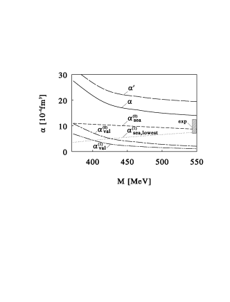
Figure 17: Electric polarizability of the nucleon of the SU(2) NJL model (Nikolov et al., 1994) as a function of the constituent quark mass $M$. The $\alpha^{\prime}$ indicates the direct result of the NJL model, the $\alpha$ incorporates corrections due to $N-\Delta$ mass splitting. The polarizability of the nucleon is defined as $\alpha=(\alpha_{p}+\alpha_{n})/2$.

In fig. 17 we present the results (Nikolov et al., 1994) for the average electric polarizability of the proton and neutron, $\alpha\equiv{1\over 2}(\alpha_{p}+\alpha_{n})$ obtained in the NJL model as a function of the constituent quark mass $M$. The different contributions as well as the total nucleon electric polarizability are presented. The long-dashed line corresponds to $\alpha^{\prime}=\alpha^{(0)}_{\rm sea}+\alpha^{(0)}_{\rm val}+\alpha^{(1)}_{\rm sea,lowest}+\alpha^{(1)}_{\rm val}$ and this is the direct result of the NJL model. The solid line shows the total $\alpha$, roughly corrected for the effects of the $N$-$\Delta$ mass splitting. For values of $M$ in the physically relevant range 400–450 MeV the changes of $\alpha$ with $M$ are small. The present results are in qualitative agreement with the results of other models (Weiner and Weise, 1985, Broniowski and Cohen, 1993) with explicit pion degrees of freedom.

The sea contributions clearly dominate over the valence ones both on leading order in $N_{c}$ and for the rotational $1/N_{c}$ corrections. These contributions are very well reproduced by the leading two terms in the gradient expansion and the first term is the so called “seagull” contribution to $\alpha$, discussed in many previous papers.

The inclusion of rotational corrections has important phenomenological consequences. The dominant contribution to the electric polarizability is obtained from pion tail effects, and is proportional to the axial constant $g_{A}^{2}$. Since the rotational corrections have been shown (Christov et al., 1994) to be crucial for reproducing the experimental value of $g_{A}$ in the model, it is important to take into account these rotational corrections for the electric polarizability. The calculation shows that indeed the rotational corrections give a sizeable contribution of about 50–60% of the leading-$N_{c}$ result. After including approximately the corrections due to the $N$-$\Delta$ mass splitting, the theoretical value is closer to experiment than in other studies in soliton models. For the typical choice of the constituent quark mass $M=420\ \rm{MeV}$ we obtain $\alpha^{\prime}\simeq 25\times 10^{-4}\ {\rm fm}^{3}$ and $\alpha\simeq 19\times 10^{-4}\ {\rm fm}^{3}$, compared to the experimental value $\alpha_{\rm exp}=9.6\pm 1.8\pm 2.2\times 10^{-4}\ \rm fm^{3}$ (Federspiel et al., 1991, Zieger et al., 1992, Schmiedmayer et al., 1991). The model prediction is, however, still too large indicating that the inclusion of other $1/N_{c}$ effects (such as e.g. meson loops) is necessary. In other approaches like e.g. the chiral perturbation theory with nucleons (for review see (Bernard et al., 1995)) the pion loops provide the main effect. In our model, parts of those meson effects are taken into account already in the leading $1/N_{c}$ order due to the presence of the mean-field. The effects of meson loops in the next to leading order in $1/N_{c}$ remains to be investigated. In particular, one hopes that the meson-loop $1/N_{c}$ effects related to the zero modes would lead to a reduction in the case of the electric polarizability.

5 SU(3)-NJL model

In the previous chapters, we have reviewed the Nambu–Jona-Lasinio model with scalar isoscalar and pseudoscalar isovector couplings. The extension of this model to the larger symmetry of SU(3) introduces not only the kaon and eta mesons to the model but offers in the baryon sector, which is the main concern of the present article, the possibility to calculate the properties of strange baryons as well as the contributions of strange quarks to the properties of the nucleon and Delta. In fact, at present these effects are in the case of the spin structure functions or the strange vector form factors under vivid discussion.

We start with a very short review of the mesonic sector which is already extensively discussed in the reviews of Klevansky (1992), Vogl and Weise (1991) and Hatsuda and Kunihiro (1994). After performing the bosonization and saddle-point approximation we fix the parameters of the model by reproducing pion and kaon properties and have again the constituent quark mass of the non-strange quarks as the only free parameter. Actually, the extension from SU(2) to SU(3) is formally not trivial, since the current mass of the strange quark, $m_{s}$, is noticeably larger than that of the up and down quarks, $m_{u}$ and $m_{d}$. This corresponds to a non-negligible explicit breaking of the SU(3)-symmetry which plays an important role in the baryon sector. We remind that the semiclassical treatment of the NJL model is justified in the large $N_{c}$ limit. In the SU(3) case, apart from the $1/N_{c}$ expansion one has to deal also with the expansion in powers of $m_{s}$. These expansions in two small parameters $1/N_{c}$ and $m_{s}$ are very sensitive to which limit is being taken first: $N_{c}\to\infty$ or $m_{s}\to 0$. This leads to certain difficulties in the collective quantization of the soliton rotation. We discuss the perturbative approaches (Weigel et al., 1992, Blotz et al., 1992, 1993a), which in view of explicit calculations of baryonic observables are most far developed at the present time. Special emphasis then is put on the possible representations of the collective hamiltonian. After a discussion of the mass spectra of the hyperon multiplets in SU(3) we review baryonic observables like the electromagnetic form factors, sigma terms, axial vector couplings, spin properties of the proton and the Gottfried sum rule. Predictions will be done for the nucleon strange form factors.

Besides the perturbative approach one can also consider the hyperons as bound states of kaon mesons in the background field of the SU(2) soliton. This approach has been invented by the Callan and Klebanov (1985) and has been applied in the chiral sigma model by McGovern and Birse (1990) and in the case of the NJL model by Weigel et al. (1994).

5.1 Extension of the NJL model to SU(3) flavors

An extension of the SU(2) flavor NJL lagrangian (1) to SU(3) can be done by a direct generalization ($\tau^{a}\to\lambda^{a}$) of the SU(2) case with scalar and pseudoscalar couplings. Then the simplest SU(3) form of a four-fermion interaction with scalar and pseudoscalar couplings reads

$${\cal L}={\bar{\Psi}}(x)\left[i\hbox to0.0pt{/\hss}{\partial}-{\hat{m}}\right]\Psi(x)+{G\over 2}\sum_{a=0}^{8}\left[\left({\bar{\Psi}}(x)\lambda^{a}\Psi(x)\right)^{2}+\left({\bar{\Psi}}(x)\lambda^{a}i\gamma_{5}\Psi(x)\right)^{2}\right]$$

where the $\lambda_{a}$ are the Gell-Mann matrices with $\mbox{Sp}\lambda^{a}\lambda^{b}=2\delta_{ab}$ and the sum over the $\lambda^{a}$ matrices includes $\lambda^{0}=\sqrt{2\over 3}{\bf 1}_{3}$ as well. This form of the couplings is demanded by requiring a chiral $SU(3)_{R}\otimes~{}SU(3)_{L}$ symmetry. The mass matrix in (5) is now enlarged by the strange quark mass

$${\hat{m}}=\left(\begin{array}[]{ccc}m_{u}&0&0\\ 0&m_{d}&0\\ 0&0&m_{s}\end{array}\right)={\bar{m}}_{0}{\bf 1}+\lambda^{3}m_{3}+\lambda^{8}m_{8}$$

where ${\bar{m}}_{0}=(m_{u}+m_{d}+m_{s})/3$, $m_{3}=(m_{u}-m_{d})/2$ and $m_{8}=(m_{u}+m_{d}-2m_{s})/(2\sqrt{3})$. Note that in contrast to SU(2), where one could write a minimal lagrangian with the singlet scalar field only and a triplet of pion fields, the rank 2 of the SU(3) group compared with rank 1 of SU(2) together with chiral symmetry requires the presence of the whole nonet of scalar and pseudoscalar couplings. Using integral identities similar to eq. (15) the bosonized form of (5) reads

$${\cal L}^{\prime}={\bar{\Psi}}(x)\left(i\hbox to0.0pt{/\hss}{\partial}-{\hat{m}}-\sum_{a=0}^{8}\left(\sigma_{a}\lambda^{a}+i\gamma_{5}\pi_{a}\lambda^{a}\right)\right)\Psi(x)-{1\over 2G}\sum_{a=0}^{8}\left[\sigma_{a}^{2}+\pi_{a}^{2}\right]-{\cal L}^{\prime}_{A}[\sigma_{a},\pi_{a}]\,.$$

Here we have added ”by hand” an extra term ${\cal L}^{\prime}_{A}[\sigma_{a},\pi_{a}]$. The necessity of this additional term is related to the U${}_{A}(1)$ problem. Besides $SU(3)_{R}\otimes~{}SU(3)_{L}\otimes~{}U_{V}(1)$ symmetry, the lagrangian ${\cal L}$ (5) has in addition the $U_{A}(1)$ symmetry. On the other hand, it is well know that in QCD the $U_{A}(1)$ symmetry is broken by the anomaly. As a consequences the $\eta^{\prime}$ meson remains massive even in the chiral limit. This means the effective low energy theory should contain some term ${\cal L}^{\prime}_{A}[\sigma_{a},\pi_{a}]$ explicitly breaking the $U_{A}(1)$ symmetry. In fact, we use the presence of ${\cal L}^{\prime}_{A}$ as an argument to consider $\eta^{\prime}$ massive and not as a Goldstone boson. For the fixing of the parameters of the NJL model only Goldstone bosons are needed. In the baryonic sector, we will use the chiral circle (5) and hence the detailed structure of ${\cal L}^{\prime}_{A}$ is irrelevant for our considerations.

After integrating over the quark fields the partition function in Euclidean space is given by

$$Z=\int{\cal D}\sigma_{a}{\cal D}\pi_{a}e^{-S(\sigma,\pi)}$$

where

$$S(\sigma,\pi)=-N_{c}{\rm Tr}\ \log D(\sigma,\pi)+{1\over 2G}\int d^{4}x\sum_{a=0}^{8}\left(\sigma_{a}^{2}+\pi_{a}^{2}\right)+\int d^{4}x{\cal L}^{\prime}_{A}[\sigma_{a},\pi_{a}]$$

with $D(\sigma,\pi)=\partial_{\tau}+h$ and

$$h=-i\gamma_{0}\gamma^{k}\partial_{k}+\gamma_{0}{\hat{m}}+\gamma_{0}\sum_{a=0}^{8}\left(\sigma_{a}\lambda^{a}+i\gamma_{5}\pi_{a}\lambda^{a}\right)\,.$$

5.2 Vacuum solutions and fixing of parameters

In the vacuum we make again a saddle point approximation similar to eq. (28)

$${{\delta S(\sigma,\pi)\over\delta\sigma_{a}}=0\ \vrule height=14.0pt,depth=7.0pt\ }_{\sigma_{a}=\sigma_{ac}\atop\pi_{a}=\pi_{ac}}\ \ \ {{\delta S(\sigma,\pi)\over\delta\pi_{a}}=0\ \vrule height=14.0pt,depth=7.0pt\ }_{\sigma_{a}=\sigma_{ac}\atop\pi_{a}=\pi_{ac}}\,.$$

For three flavors there are the $\sigma_{0}$, $\sigma_{3}$ and $\sigma_{8}$ fields which can have non-vanishing vacuum expectation values. Therefore, instead of eq. (44) one has in general one gap equation for each flavor degree of freedom. Neglecting isospin breaking (${m_{0}}=m_{u}=m_{d}$) in the following the non-trivial gap equations read

$${1\over G}\sigma_{1}-8N_{c}\sigma_{1}I_{1}(\sigma_{1}) = {{m_{0}}\over G}$$

$${1\over G}\sigma_{2}-8N_{c}\sigma_{2}I_{1}(\sigma_{2}) = {m_{s}\over G}$$ (262)

where we set $\sigma_{1}=\sqrt{2\over 3}\sigma_{0c}+{1\over\sqrt{3}}\sigma_{8c}+{m_{0}}$ and $\sigma_{2}=\sqrt{2\over 3}\sigma_{0c}-{2\over\sqrt{3}}\sigma_{8c}+m_{s}$. Deriving these equations we neglected the contribution of the ${\cal L}^{\prime}_{A}[\sigma_{a},\pi_{a}]$.

The spontaneous breaking of chiral symmetry leads now to the appearance of constituent quark masses for the non-strange and strange sector according to

$$M_{u}=M_{d}=\sigma_{1},\ \ \ \ \ M_{s}=\sigma_{2}\,.$$

This resembles two independent Dirac equations with mass gaps $M_{u}$ and $M_{s}$. In addition, there are two quark condensates

$$<{\bar{u}}u>\>=\><{\bar{d}}d> = -{1\over V_{4}}\,{1\over 2}{\partial\over\partial{m_{0}}}Z$$

$$<{\bar{s}}s> = -{1\over V_{4}}{\partial\over\partial m_{s}}Z$$ (263)

which become equal in the chiral limit and actually are of the order of $-(250\,\mbox{MeV})^{3}$. Using the gap equations eqs. (262) the eqs. (263) can be cast into the form

$$<{\bar{u}}u+{\bar{d}}d> = -{1\over G}\left(M_{u}-{m_{0}}\right)$$

$$<{\bar{s}}s> = -{1\over 2G}\left(M_{s}-m_{s}\right)\,.$$ (264)

Similarly to the definition of the pion decay constant in eq. (70), we can define the corresponding vacuum matrix element of the axial vector current $A_{\mu}^{a},\>a=4,5,6,7$ with the physical kaon fields $\pi_{a},\>a=4,5,6,7$. As a result one obtains (Schneider et al., 1995)

$$f_{\pi} = M_{u}g_{\pi}Z_{p}(q^{2}=-m_{\pi}^{2})$$

$$f_{K} = {M_{s}+M_{u}\over 2}g_{K}Z_{p}(q^{2}=-m_{K}^{2})$$ (265)

where $g_{K}$ can be determined from the corresponding eq. (61). In the chiral limit, from the (264) and the gap equation (262) it follows that

$$f_{\pi}=f_{K}=M_{u}g_{\pi}Z_{p}(q^{2}=0)$$

and

$${m_{K}^{2}\over m_{\pi}^{2}}={m_{s}+m_{0}\over 2{m_{0}}}\,.$$

For finite quark current masses the kaon decay constant deviates from the pion decay constant but however it is still underestimated by 10 %.

The masses of the pion and kaon are determined from the two-point meson functions (50)

$$m_{\pi}^{2} = {{m_{0}}\over GM_{u}Z_{p}(q^{2}=-m_{\pi}^{2})}$$

$$m_{K}^{2} = \left({m_{s}\over M_{s}}+{{m_{0}}\over M_{u}}\right){1\over 2GZ_{p}(q^{2}=-m_{K}^{2})}+\Delta^{2}_{M_{s}}$$ (266)

with $\Delta_{M_{s}}=M_{s}-M_{u}$.

Fixing of the parameters. The SU(3) NJL model in the present form contains four unknown parameters: the coupling constant $G$, the current quark masses $m_{0}$ and $m_{s}$, and the regularization cut-off $\Lambda$. First, instead of $G$ the constituent quark mass $M_{u}$ is used as parameter which is related to $G$ by the first gap equation (262). Second, for a given $M_{u}$ the $m_{0}$, $m_{s}$ and $\Lambda$ are fixed to reproduce $f_{\pi}=93$ MeV, $m_{\pi}=139$ MeV and the kaon mass $m_{K}=496$ MeV. The $M_{u}$ is not fixed in the meson sector but in the baryon sector, in order to reproduce best the experimental data of the nucleon. This results, as in SU(2), in preferred values of $M_{u}$ about 420 MeV. The strange constituent mass $M_{s}$ is not an independent quantity but determined by $M_{u}$ according to the second gap equation (262).

In contrast to the SU(2) case, where the average current quark mass $m_{0}$ is rather small and the results do not depend on its particular value fixed by the physical pion mass, in the SU(3) case, the explicit chiral symmetry breaking due to the strange current mass $m_{s}\approx 175$ MeV (Bijnens et al., 1995) will be treated perturbatively up to the second order corrections in $m_{s}$. Apparently we need to reproduce the value of the strange quark current mass properly. Actually, if one follows the above scheme and uses the proper time regularization (41) with $\phi(u)=\theta({1\over\Lambda^{2}}-u)$, the absolute values of $m_{u}$, $m_{d}$ and $m_{s}$ come out about two times larger than expected. To that end we make use essentially of the freedom to choose the particular form of the function $\phi(u)$ in the proper-time regulator (41) in order to adjust the quark condensate and the current quark masses to their phenomenologically accepted values. In our practical calculations we use

$$\phi(u)=c\theta(u-\Lambda_{1}^{-2})+(1-c)\theta(u-\Lambda_{2}^{-2})$$ (267)

in which two additional parameters $c$ and $\Lambda_{2}$ appear. The $c$ is used to obtain a value for $m_{0}$ of 6.1 MeV. The $\Lambda_{2}$ is chosen as small as possible in order to facilitate the numerical effort in the calculation of the soliton.

5.3 Restriction to Goldstone modes

Up to now we have considered the meson sector of SU(3) NJL in terms of independent fields $\sigma^{a}$ and $\pi^{a}$ with $a=0,1,\dots,8$. The parameters of the model are fixed by pion and kaon properties. Like in the SU(2) case the model as such does not support solitonic solutions and, again, one has to subject the field to the condition of the chiral circle. In analogy to (76) this is defined as

$$\sigma_{a}(x)\lambda^{a}+i\pi_{a}(x)\lambda^{a}=MU^{(3)}_{c}({\vec{x}})=Me^{i\pi_{a}^{\prime}\lambda^{a}}$$

where $U_{c}^{(3)^{\dagger}}({\vec{x}})U^{(3)}_{c}({\vec{x}})=1$ similar to the case of SU(2) chiral fields. The sum goes over $a=0,1,\dots,8$ and $M$ is given by $M=M_{u}$ even in the case of $M_{s}\neq M_{u}$. This is consistent with the so called trivial embedding of SU(2) into SU(3) discussed in the next subsection.

The condition of the chiral circle corresponds to a clear separation between the Goldstone degrees of freedom, i.e. pions, kaons and eta, and non-Goldstone ones like sigmas. Since we are interested in describing the ground state properties of the nucleon and the hyperons, the degrees of freedom corresponding to heavy mesons are of less importance and hence, will be ignored. With the $U_{c}^{(3)}(x)$ of eq.(5) in the solitonic sector, the present model is identical to the SU(3) version of the Chiral quark soliton model of Diakonov et al. (1988). This model is based on the instanton model of the QCD vacuum (Diakonov and Petrov, 1986). We remind that the effective quark lagrangian derived by Diakonov and Petrov (1986) from the instanton model of the QCD vacuum has a form of a ‘t Hooft-like interaction which explicitly breaks the U${}_{A}(1)$ symmetry. Its bosonization leads to meson fields of the form (5).

5.4 Trivial embedding of SU(2) hedgehog soliton into SU(3)

By analogy with the SU(2) case we expect that the low-lying baryons can be described as rotational excitations of some classical soliton solution. The spectrum of these baryons in the real world imposes certain restrictions on the symmetry of the SU(3) soliton. It was suggested by Witten (1983) that one should consider the trivial embedding of the SU(2) hedgehog soliton into SU(3)

$$U^{(3)}_{c}({\vec{x}})=\left(\begin{array}[]{ccc}U^{(2)}_{c}({\vec{x}})&\ \vrule height=14.0pt,depth=7.0pt&0\\ \hline\cr 0&\ \vrule height=14.0pt,depth=7.0pt&1\end{array}\right)$$

where $U^{(2)}_{c}({\vec{x}})=\cos\Theta(r)+i{\vec{\tau}}{\hat{x}}\sin\Theta(r)$ coincides with the SU(2) stationary meson field configuration $U_{c}({\vec{x}})$ of eq. (116). The advantage of this ansatz for the saddle point solution is that its rotational excitations naturally describe the particles of the SU(3) octet and decuplet.

If one neglects the quark masses then there is a continuous set of saddle point solutions $R^{\dagger}U^{(3)}_{c}({\vec{x}})R$ where $R$ is an arbitrary SU(3) matrix. Similarly to the SU(2) case, in the path integral scheme we have to take into account the path integral over time dependent fields of the form

$$U^{(3)}(\tau,{\vec{x}})=R(\tau)U^{(3)}_{c}({\vec{x}})R^{\dagger}(\tau)\,.$$

After this path integral is computed one arrives at the baryon rotational wave functions $\psi(R)$ depending on the SU(3) orientation matrix $R$. As in the SU(2) case the SU(3) flavor generators and the spin operator acting in the space of this rotational wave functions are nothing else but the generators of the left and right rotations of the matrix $R$. By analogy with (144), (145) we obtain

$$\exp(i\omega_{a}T_{a})\psi(R)=\psi\left(\exp(-i\omega_{a}\lambda_{a}/2)R\right)\,,$$ (268)

$$\exp(i\omega_{a}J_{a})\psi(R)=\psi\left(R\exp(i\omega_{a}\lambda_{a}/2)\right)\,.$$ (269)

Here $T_{a}$ are eight SU(3) flavor generators. As for the right generators $J_{a}$, the components with $a=1,2,3$ have the meaning of the spin operator. The other components of $J_{a}$ have no direct physical meaning. Note that under the rotation associated with $J_{8}$ the field $U^{(3)}(\tau,{\vec{x}})$ does not change. This means that the parametrization of the rotating soliton by the SU(3) matrix $R$ contains ”non-physical” degrees of freedom. As it will be seen later this leads to a constraint on the allowed eigenvalues of $J_{8}$.

5.5 Expansion in angular velocity

Restricting the path integral over $U(x)$ in ((94) to meson configurations of the form $U^{(3)}(\tau,{\vec{x}})$ (5) we obtain by analogy with (128)

$$\Pi_{B}(T)=\Gamma_{B}^{\{f\}}\Gamma_{B}^{\{g\}*}\int{\cal D}R\prod_{i=1}^{N_{c}}\langle 0,T/2\mid{1\over D(RU^{(3)}_{c}R^{\dagger})}\mid 0,-T/2\rangle_{f_{i}g_{j}}e^{-S(RU^{(3)}_{c}R^{\dagger})}$$

where the $\Gamma_{B}^{\{f\}}$ carry the quantum numbers of the hyperons and the Dirac operator in the body-fixed frame of the soliton is now given by:

$$D(U^{(3)}_{c}(\tau,{\vec{x}}))=R\left[\partial_{\tau}+h_{0}+h_{1}+i\Omega\right]R^{\dagger}\,.$$

Here $h_{0}$ is the single particle hamiltonian

$$h_{0} = -i\gamma_{0}\gamma^{k}\partial_{k}+M_{u}\gamma_{0}U^{(3)\gamma_{5}}_{c}+\gamma_{0}m_{0}{\bf 1}$$ (270)

which includes the two flavor hamiltonian eq. (79) embedded in SU(3). In contrast to SU(2) case in (5) we have additionally the term

$$h_{1}=\gamma^{0}\left({\Delta_{M_{s}}\over 3}{\bf 1}-{\Delta_{M_{s}}\over\sqrt{3}}D_{8a}^{(8)}(R(\tau))\lambda_{a}\right)$$

which appears due to the fact, that the mass matrix ${\hat{m}}$ does not commute with the rotation matrix $R(\tau)$. We also have defined

$$\Delta_{M_{s}}=M_{s}-M_{u}\,.$$

Below we consider $h_{1}$ as a perturbation. Note that there is a freedom of the redistribution of the singlet part of the strange quark mass between $h_{0}$ and $h_{1}$. Different saddle points corresponding to this freedom have been studied by Schneider et al. (1995). In the following we will discuss the case where the saddle point is determined by using hamiltonian (270) and $h_{1}$ is treated as a perturbation.

Expanding the correlation function (5) in powers of $\Omega$ and $\Delta_{M_{s}}(m_{s})$ up to the second order in the rotational velocity we get for the propagators

$$\prod_{i=1}^{N_{c}}\langle 0,T/2\mid{1\over D(RU^{(3)}_{c}R^{\dagger})}\mid 0,-T/2\rangle_{f_{i}g_{i}}{}_{\stackrel{{\scriptstyle\displaystyle\sim}}{{T\to\infty}}}$$

$$\exp{\left(-N_{c}\epsilon_{val}(U)T-{1\over 2}I_{ab}^{val}\int d\tau\Omega^{a}\Omega^{b}-{N_{c}\over 2\sqrt{3}}i\int d\tau\Omega^{8}-\int d\tau L_{val}[\Delta_{M_{s}}]\right)}$$ (271)

as well as from the effective action

$$\exp(-S(RU^{(3)}_{c}R^{\dagger}))=\exp{\left(-TE_{sea}(U)-{1\over 2}I_{ab}^{sea}\int d\tau\Omega^{a}\Omega^{b}-\int d\tau L_{sea}[\Delta_{M_{s}}]\right)}$$

where $L[\Delta_{M_{s}}]=L_{sea}[\Delta_{M_{s}}]+L_{val}[\Delta_{M_{s}}]=O(\Delta_{M_{s}})$ and will be discussed below. The tensor of the moments of inertia $I_{ab}$ is diagonal but in contrast to the SU(2) case its components are different

$$I_{ab}=\left\{\begin{array}[]{l}I_{1},\>a=b=1,2,3\\ I_{2},\>a=b=4,5,6,7\\ 0,\>{\rm otherwise.}\end{array}\right.$$

The second important difference from the SU(2) case is the linear term in $\Omega^{8}$ in (271). In Skyrme type models, this expression is proportional to the topological winding number of the chiral field which in these models coincides with the baryon number. In the present non-topological chiral model the term with $\Omega^{8}$ is due to the discrete valence level in the Dirac spectrum. The presence of the $\Omega^{8}$ term is a reflection of the fact that right rotations associated with the generator $J_{8}$ have no effect on the chiral field. Therefore, the generator $J_{8}$ corresponding the rotational velocity $\Omega^{8}$ is constrained. From the term linear in $\Omega^{8}$ in eq. (271) we see that

$$J_{8}=-{N_{c}\over 2\sqrt{3}}\,.$$

By analogy with the hypercharge

$$Y=(2/\sqrt{3})T_{8}\,,$$

one can introduce the ”right” hypercharge

$$Y_{R}=(2/\sqrt{3})J_{8}\,,$$

in terms of which the constraint (5) can be rewritten in the form

$$Y_{R}=-N_{c}/3\,.$$

This in turn transforms into a constraint for the possible representations of SU(3). Actually, one can show that only representations with zero triality survive. These are the octet and decuplet representations with spin $1/2$ and $3/2$ respectively.

By analogy with the case of the SU(2) case the effective rotational lagrangian leads to the following quantization rules

$$J_{a}=\left\{\begin{array}[]{ll}i{\Omega^{a}I_{1}},&a=1,2,3\\ i{\Omega^{a}I_{2}},&a=4,5,6,7\\ {\sqrt{3}\over 2}Y_{R}=-{N_{c}\over 2\sqrt{3}},&a=8\,.\end{array}\right.$$

Here, the components $J_{a}$ with $a=1,2,3$ correspond to the spin operator. Using these quantization rules we obtain a collective hamiltonian from (271) and (5) in the form

$$H_{coll}^{(0)}={1\over 2}\left({1\over I_{1}}-{1\over I_{2}}\right){\cal C}_{2}(SU(2))+{1\over 2I_{2}}{\cal C}_{2}(SU(3))-{3\over 8I_{2}}\,.$$

Here

$${\cal C}_{2}(SU(3))=\sum\limits_{a=1}^{8}J_{a}^{2}=\sum\limits_{a=1}^{8}T_{a}^{2}$$ (272)

is the quadratic Casimir operator of the SU(3) group and

$${\cal C}_{2}(SU(2))=\sum\limits_{a=1}^{3}J_{a}^{2}$$ (273)

is the Casimir operator of the SU(2) subgroup corresponding to spin generators $J_{a}$ $(a=1,2,3)$.

The upper index $(0)$ in $H_{coll}^{(0)}$ indicates that we are working in the chiral limit without any mass corrections. Those will be incorporated later and will yield additional terms $H_{coll}^{(1)}$ and $H_{coll}^{(2)}$.

The Hamiltonian $H_{coll}^{(0)}$ commutes with all flavor SU(3) generators $T_{a}$. Therefore the eigenstates of $H_{coll}^{(0)}$ can be classified according to the irreducible representations of SU(3). Below we use the well known $(p,q)$ parametrization the SU(3) representations in which the octet is $(1,1)$ and the decuplet is $(3,0)$.

Since in our model the spin $J_{a}$ and flavor $T_{a}$ operators are realized as the generators of right and left rotations of the same orientation matrix $R$, the representation $(p,q)$ should be the same for $T_{a}$ and for $J_{a}$. Apart from the representation $(p,q)$ the eigenstates of $H_{coll}^{(0)}$ are also characterized by the quantum numbers corresponding to the following set of commuting operators:

$$Y={2\over\sqrt{3}}T_{8},\qquad\sum\limits_{a=1}^{3}T_{a}^{2},\qquad T_{3}\,,$$

$$Y_{R}={2\over\sqrt{3}}J_{8},\qquad\sum\limits_{a=1}^{3}J_{a}^{2},\qquad J_{3}\,.$$ (274)

The corresponding wave functions are

$$\psi_{(Y,T,T_{3})(Y_{R},J,J_{3})}^{(p,q)}(R)=\sqrt{\mbox{dim}(p,q)}\,(-1)^{Y_{R}/2+J_{3}}D_{(Y,T,T_{3})(-Y_{R},J,-J_{3})}^{(p,q)\ast}(R)$$ (275)

where the asterisk stands for the complex conjugation and $\mbox{dim}(p,q)$ is the dimension of the representation $(p,q)$.

With these wave functions the Casimir operator has the following spectrum

$${\cal C}_{2}(SU(3))\psi_{Y,T,T_{3};Y_{R},J,J_{3}}^{(p,q)}={1\over 3}(p^{2}+q^{2}+3(p+q)+pq)\psi_{(Y,T,T_{3})(Y_{R},J,J_{3})}^{(p,q)}\,,$$ (276)

$${\cal C}_{2}(SU(2))\psi_{(Y,T,T_{3})(Y_{R},J,J_{3})}^{(p,q)}=J(J+1)\psi_{(Y,T,T_{3})(Y_{R},J,J_{3})}^{(p,q)}\,.$$ (277)

In the chiral limit presently considered, the members of each multiplet are degenerate in energy. Using (276), (277) we find the eigenvalues of the rotational hamiltonian (5) which leads to the following result for the energy of the center of the multiplets, defined as the average mass of all the members,

$$E_{p,q,J}=M_{cl}+{1\over 2}\left({1\over I_{1}}-{1\over I_{2}}\right)J(J+1)+{1\over 6I_{2}}\left(p^{2}+q^{2}+3(p+q)+pq\right)-{3\over 8I_{2}}\,.$$

Note that constraint (5) fixes the spin of the particles of the $(p,q)$ multiplet. The analog of the nucleon delta splitting (155) has to be interpreted in SU(3) as octet and decuplet-splitting, i.e. the energy difference between the centers of the octet and decuplet, and follows as

$$E_{8-10}=E_{3,0,3/2}-E_{1,1,1/2}={3\over 2I_{1}}\,.$$

Formally this coincides with $E_{N\Delta}$ in SU(2), however, the phenomenological value for the difference of the average octet and decuplet masses is now $E_{8-10}^{ph}=230\mbox{MeV}$.

5.6 Strange mass terms of the collective lagrangian

In order to calculate the splitting within the multiplets we have to include the SU(3) symmetry breaking terms due to $h_{1}$ in (5). Note that we deal with two quantities which may be considered as small quantities. The first one is the rotational velocity $\Omega$, which is of the order of $1/N_{c}$. The second one is the mass difference $\Delta_{M_{s}}=M_{s}-M_{u}$. Assuming both corrections to be roughly of the same order we use systematic expansions up to the second order.

Expanding the baryon correlator (5) and considering sea and valence contributions together, one obtains for $L[\Delta_{M_{s}}]$ in (271) and (5)

$$L[\Delta_{M_{s}}] = L_{1}[\Delta_{M_{s}}]+L_{2}[\Delta_{M_{s}},\Omega]$$ (278)

$$+L_{3}[\Delta_{M_{s}}^{2}]+O\left(\Delta_{M_{s}}^{m}\Omega^{n}\right)\ \ \ m+n\geq 3\,.$$

The first term in this expansion

$$L_{1}[\Delta_{M_{s}}]={\sigma\over{m_{0}}}{\Delta_{M_{s}}\over 3}\left(1-D_{88}^{(8)}(R(\tau))\right)$$

contains the SU(2) sigma term $\sigma$, which in the present model is given by

$$\sigma={m_{0}}{{\partial M_{cl}[{m_{0}}]\over\partial{m_{0}}}\ \vrule height=14.0pt,depth=7.0pt\ }_{{m_{0}}=0}\,.$$

Then we have in the next order $O\left(\Omega\Delta_{M_{s}}\right)$

$$L_{2}[\Delta_{M_{s}},\Omega] = {\Delta_{M_{s}}\over\sqrt{3}}2K_{1}\sum_{i=1}^{3}D_{8i}^{(8)}(R(\tau))\Omega_{i}(\tau)$$ (279)

$$+{\Delta_{M_{s}}\over\sqrt{3}}2K_{2}\sum_{a=4}^{7}D_{8a}^{(8)}(R(\tau))\Omega_{a}(\tau)\,,$$

where $K_{1}$ and $K_{2}$ similar to $I_{1},I_{2}$ are related to tensor $K_{ab}$

$$K_{ab}=\left\{\begin{array}[]{ll}K_{1},&a=b=1,2,3\\ K_{2},&a=b=4,5,6,7\\ 0,&{\rm otherwise.}\end{array}\right.$$

The latter can be split in valence

$$K_{ab}^{val}={N_{c}\over 2}\sum_{n\neq m}{\langle val\mid\lambda^{a}\mid n\rangle\langle n\mid\lambda^{b}\gamma_{0}\mid val\rangle\over\epsilon_{n}-\epsilon_{val}}\,.$$

and sea part

$$K_{ab}^{sea}={N_{c}\over 4}\sum_{\epsilon_{n}>0\atop\epsilon_{m}<0}{\langle m\mid\lambda^{a}\mid n\rangle\langle n\mid\lambda^{b}\gamma_{0}\mid m\rangle\over\epsilon_{n}-\epsilon_{m}}$$

In contrast to the sea contributions of $I_{1}$ and $I_{2}$ that of $K_{ab}$ originates from the imaginary part of the effective euclidean action. Hence, it is ultraviolet finite and needs no regularization. One should note that in Skyrme approaches with vector mesons such contributions from the effective action are obtained only by adding the gauged Wess-Zumino term (Park and Weigel, 1991).

From the quadratic corrections in the symmetry breaking we obtain

$$L_{3}[\Delta_{M_{s}}^{2}] = \left({\Delta_{M_{s}}\over\sqrt{3}}\right)^{2}2N_{1}\sum_{i=1}^{3}D_{8i}^{(8)}(R(\tau))D_{8i}^{(8)}(R(\tau))$$ (280)

$$+\left({\Delta_{M_{s}}\over\sqrt{3}}\right)^{2}2N_{2}\sum_{a=4}^{7}D_{8a}^{(8)}(R(\tau))D_{8a}^{(8)}(R(\tau))$$

$$+\left({\Delta_{M_{s}}\over\sqrt{3}}\right)^{2}{2\over 3}N_{0}\left(1-D_{88}^{(8)}(R(\tau))\right)\left(1-D_{88}^{(8)}(R(\tau))\right)\,,$$

where $N_{1}$ and $N_{2}$ are diagonal elements of tensor $N_{ab}$

$$N_{ab}=\left\{\begin{array}[]{l}N_{1},\qquad a=b=1,2,3\\ N_{2},\qquad a=b=4,5,6,7\\ N_{0},\qquad a=b=8\,.\end{array}\right.$$

It consists of a valence part

$$N_{ab}^{val}={N_{c}\over 2}\sum_{n\neq val}{\langle val\mid\lambda^{a}\gamma_{0}\mid n\rangle\langle n\mid\lambda^{b}\gamma_{0}\mid val\rangle\over E_{n}-E_{val}}$$

and a regularized sea contribution

$$N_{ab}^{sea}={N_{c}\over 4}\sum_{n,m}\langle m\mid\lambda^{a}\gamma_{0}\mid n\rangle\langle n\mid\lambda^{b}\gamma_{0}\mid m\rangle{\cal R}_{N}^{\Lambda}(\epsilon_{n},\epsilon_{m})\,.$$

The regularization function ${\cal R}_{N}^{\Lambda}$ is given by

$${\cal R}_{N}^{\Lambda}(\epsilon_{n},\epsilon_{m})={1\over 2\sqrt{\pi}}\int_{0}^{\infty}{du\over\sqrt{u}}\phi(u)\left[{\epsilon_{n}e^{-u\epsilon_{n}^{2}}-\epsilon_{m}e^{-u\epsilon_{m}^{2}}\over\epsilon_{n}-\epsilon_{m}}\right]\,.$$

Before we can study the mass splittings from the collective hamiltonian resulting from (280) , one has to remember that in the presence of the linear terms in the rotational velocity $\Omega$, the generators of the group are modified according to

$$J_{a}=\left\{\begin{array}[]{ll}i{\Omega^{a}I_{1}}-2{\Delta_{M_{s}}\over\sqrt{3}}K_{1}D_{8a}^{(8)}(R(\tau)),&a=1,2,3\\ i{\Omega^{a}I_{2}}-2{\Delta_{M_{s}}\over\sqrt{3}}K_{2}D_{8a}^{(8)}(R(\tau)),&a=4,5,6,7\\ -{N_{c}\over 2\sqrt{3}}={\sqrt{3}\over 2}Y_{R},&a=8\,.\end{array}\right.$$

5.7 Hyperon splittings in linear order - Sum rules

Here, we consider the hyperon splitting of the octet and decuplet in linear order in $\Delta_{M_{s}}$ and neglect the isospin breaking, i.e. set $m_{u}=m_{d}=m_{0}$. As shown in the meson sector in linear order of $\Delta_{M_{s}}$ the difference $M_{s}-{M_{u}}$ equals $m_{s}$. Now the collective Hamiltonian

$$H_{coll}=H_{coll}^{(0)}+H_{coll}^{(1)}$$

includes a new term

$$H_{coll}^{(1)} = {\sigma\over{m_{0}}}{m_{s}\over 3}\left(1-D_{88}^{(8)}(R)\right)+{2m_{s}\over\sqrt{3}}\left({K_{1}\over I_{1}}-{K_{2}\over I_{2}}\right)\sum_{i=1}^{3}D_{8i}^{(8)}(R)J_{i}$$ (281)

$$-{m_{s}}{K_{2}\over I_{2}}Y+{N_{c}m_{s}\over 3}{K_{2}\over I_{2}}D_{88}^{(8)}(R)\,.$$

The moments of inertia and the matrix elements of the Wigner functions can be found in (Blotz et al., 1993a).

Although $H_{coll}^{(1)}$ contains three different operators $Y,D_{88}^{(8)}(R)$ and $\sum_{i=1}^{3}D_{8i}^{(8)}(R)J_{i}$, the mass splitting can be parametrized in terms the two quantities

$$\Delta^{hyp}={1\over 3}{m_{s}\over{m_{0}}}\sigma+m_{s}\left(2{K_{2}\over I_{2}}-3{K_{1}\over I_{1}}\right)$$

and

$$\delta^{hyp}=m_{s}{K_{1}\over I_{1}}\,.$$

For the masses of the octet and decuplet baryons, calculated relative to the mass of the $\Sigma^{*}$, one gets (Blotz et al., 1993a)

$$\begin{array}[]{lllrlrll}&\Delta m_{N}&=&-{3\over 10}&\Delta^{hyp}&-&\delta^{hyp}&-E_{8-10}\\ &\Delta m_{\Lambda}&=&-{1\over 10}&\Delta^{hyp}&&&-E_{8-10}\\ &\Delta m_{\Sigma}&=&{1\over 10}&\Delta^{hyp}&&&-E_{8-10}\\ &\Delta m_{\Xi}&=&{1\over 5}&\Delta^{hyp}&+&\delta^{hyp}&-E_{8-10}\\ &\Delta m_{\Delta}&=&-{1\over 8}&\Delta^{hyp}&-&\delta^{hyp}&\\ &\Delta m_{\Sigma^{*}}&=&0&&&\\ &\Delta m_{\Xi^{*}}&=&{1\over 8}&\Delta^{hyp}&+&\delta^{hyp}&\\ &\Delta m_{\Omega}&=&{1\over 4}&\Delta^{hyp}&+&2\delta^{hyp}&\\ \end{array}$$

The reason that we consider the mass spectrum relative to the $\Sigma^{*}$ is that the mass of the $\Sigma^{*}$ almost corresponds to the center of the mass of the decuplet. From the formulas (LABEL:c6pl) above, it follows the mass relation of Guadagnini (1984)

$$m_{\Xi^{*}}-m_{\Sigma^{*}}+m_{N}={1\over 8}(11m_{\Lambda}-3m_{\Sigma})\,.$$

Here it is interesting to note that this sum rule can be obtained in the pseudoscalar Skyrme model only by introducing the hypercharge operator by hand with some unknown coefficients. In the present approach, this term arises naturally (281).

Furthermore, one obtains also the Gell-Mann – Okubo relations

$${3\over 4}m_{\Lambda}+{1\over 4}m_{\Sigma}={1\over 2}(m_{N}+m_{\Xi})$$

and

$$m_{\Omega}-m_{\Xi^{*}}=m_{\Xi^{*}}-m_{\Sigma^{*}}=m_{\Sigma^{*}}-m_{\Delta}\,.$$

It should be noted that these relations are mass sum rules which rely basically on the fact, that the SU(3) flavor symmetry breaking part of the strong interaction can be treated in first order perturbation theory. Their validity shows in some way the consistency of the quantization procedure. On the other hand the values of the hyperon masses themselves depend on the dynamics of the present model and this goes beyond the perturbative sum rule approach.

5.8 Hyperon splitting in second order - Wave functions

In the present scheme, the corrections in second order of the strange quark mass have three different origins. The first one results from the expansion of the baryon correlator in $\Delta_{M_{s}}=M_{s}-M_{u}$. The second one is due to the quantization formulas (5) , which replace the angular velocities in (280) by the corresponding generators. Accordingly, the collective hamiltonian contains not only

$$H_{coll}^{(1)} = {\sigma\over{m_{0}}}{\Delta_{M_{s}}\over 3}\left(1-D_{88}^{(8)}(R)\right)$$ (282)

$$+{2\Delta_{M_{s}}\over\sqrt{3}}{K_{1}\over I_{1}}\sum_{i=1}^{3}D_{8i}^{(8)}(R)J_{i}+{2\Delta_{M_{s}}\over\sqrt{3}}{K_{2}\over I_{2}}\sum_{a=4}^{7}D_{8a}^{(8)}(R)J_{a}$$

but also second order terms in the $\Delta_{M_{s}}(m_{s})$

$$H_{coll}^{(2)} = 2{\Delta_{M_{s}}^{2}\over 3}{K_{1}^{2}\over I_{1}}\sum_{i=1}^{3}D_{8i}^{(8)}(R)D_{8i}^{(8)}(R)+2{\Delta_{M_{s}}^{2}\over 3}{K_{2}^{2}\over I_{2}}\sum_{a=4}^{7}D_{8a}^{(8)}(R)D_{8a}^{(8)}(R)$$ (283)

$$-2N_{1}{\Delta_{M_{s}}^{2}\over 3}\sum_{i=1}^{3}D_{8i}^{(8)}(R)D_{8i}^{(8)}(R)-2N_{2}{\Delta_{M_{s}}^{2}\over 3}\sum_{a=4}^{7}D_{8a}^{(8)}(R)D_{8a}^{(8)}(R)$$

$$-2N_{0}{\Delta_{M_{s}}^{2}\over 3}\left(1-D_{88}^{(8)}(R)\right)^{2}\,.$$

To study the third contribution in second order of the symmetry breaking we recall the perturbation theory for our system of $H_{coll}^{(0)}+H_{coll}^{(1)}+H_{coll}^{(2)}$. For the energy of a baryon $B$ in the representation $[n]$, which has to be the lowest dimensional one where the quantum numbers of the baryon appears, we can write in increasing order of the perturbation:

$$E_{B,n}^{(0)} = \langle B,n\mid H_{coll}^{(0)}\mid B,n\rangle$$ (284)

$$E_{B,n}^{(1)} = \langle B,n\mid H_{coll}^{(1)}\mid B,n\rangle$$ (285)

$$E_{B,n}^{(2)} = \langle B,n\mid H_{coll}^{(2)}\mid B,n\rangle+\sum_{n\neq n^{\prime}}{\mid\langle B,n^{\prime}\mid H_{coll}^{(1)}\mid B,n\rangle\mid^{2}\over E_{B,n}^{(0)}-E_{B,n^{\prime}}^{(0)}}\,.$$ (286)

Here, $E_{B,n}^{(m)}$ is the energy of baryon of quantum numbers $B$ in the representation $[n]$ with strangeness corrections of the order $m$ taken into account. In the lowest order the energies $E_{B,n}^{(0)}$ (284) are degenerate for each multiplet and correspond to the mass center of the multiplet. In the next order $E_{B,n}^{(1)}$ include linear strange mass contributions from the matrix elements of $H_{coll}^{(1)}$ between the unperturbed wave functions $\mid B,n\rangle$. This removes the degeneracy for the zero-order results $E_{B,n}^{(0)}$. The second-order contributions $E_{B,n}^{(2)}$ (286) are from $H_{coll}^{(2)}$ between the wave functions of lowest order as well as from the last term in (286) . There the summation is over all representations $[n^{\prime}]\neq[n]$. In fact, this term appears since the baryon wave-functions of the collective hamiltonian $H_{coll}^{(0)}+H_{coll}^{(1)}$ after diagonalization in the space of all $\mid B,n\rangle$ are no longer pure octet or decuplet states. Because the operator $H_{coll}^{(1)}$ commutes with $Y,T,T_{3}$ and $J$ operators, there are in addition only higher representations like $[{\bar{1}0}]$ of $[27]$ in the case of octet baryons and $[27]$ and $[35]$ in the case of decuplet ones. These higher representations enter the baryon wave functions implicit in (286) perturbatively in first order of the symmetry breaking and therefore the total contribution to the energy in (286) is quadratic in the symmetry breaking.

Actually, if the baryon is a member of the octet, the only non-vanishing matrix elements can be parametrized by the quantum numbers of the baryons according to

$$\mid\langle B,{\bar{10}}\mid H_{coll}^{(1)}\mid B,8\rangle\mid^{2}={1\over 40}\left(\alpha+\gamma{1\over 2}\right)^{2}\left(Y+{1\over 4}Y^{2}+T(T+1)\right)$$

and

$$\mid\langle B,{{27}}\mid H_{coll}^{(1)}\mid B,8\rangle\mid^{2}={1\over 100}\left(\alpha-\gamma{1\over 6}\right)^{2}\left(9+{5\over 2}\left(T(T+1)-{1\over 4}Y^{2}\right)-{7\over 4}Y^{2}\right)$$

with the abbreviations

$$\alpha = -{1\over 3}{\Delta_{M_{s}}\over{m_{0}}}\sigma+{K_{2}\over I_{2}}\Delta_{M_{s}}$$

$$\beta = -\Delta_{M_{s}}{K_{2}\over I_{2}}$$

$$\gamma = 2\Delta_{M_{s}}\left({K_{1}\over I_{1}}-{K_{2}\over I_{2}}\right)\,.$$ (287)

Similarly, if the baryon is in the decuplet, the only non-vanishing matrix elements are given by

$$\langle B,27\mid H_{coll}^{(1)}\mid B,10\rangle={1\over 16}\left(\alpha+\gamma{5\over 6}\right)^{2}\left(1+{3\over 4}Y+{1\over 8}Y^{2}\right)$$

and

$$\langle B,35\mid H_{coll}^{(1)}\mid B,10\rangle={5\over 112}\left(\alpha-{1\over 2}\gamma\right)^{2}\left(1-{1\over 4}Y-{1\over 8}Y^{2}\right)\,.$$

We will consider expectation values of external current operators, for which we need also the wave function $\mid B\rangle$ itself in the next to leading order of the symmetry breaking. Then the wave functions can be written in first order perturbation theory as

$$\mid B\rangle=\mid n,B\rangle+\sum_{n\neq n^{\prime}}\mid n^{\prime},B\rangle{\langle B,n^{\prime}\mid H_{coll}^{(1)}\mid B,n\rangle\over E_{B,n}^{(0)}-E_{B,n^{\prime}}^{(0)}}\,.$$

Furthermore, the wave functions for the octet baryons, which will be the case of special interest in the next sections, in linear approximation in $\Delta_{M_{s}}$ read

$$\mid B\rangle = \mid B,8\rangle-{I_{2}\over 6\sqrt{5}}\left(\alpha+{1\over 2}\gamma\right)\left(Y+{1\over 4}Y^{2}+T(T+1)\right)\mid B,{\bar{10}}\rangle$$ (288)

$$-{2I_{2}\over 50}\left(\alpha-{1\over 6}\gamma\right)\left(\sqrt{6}Y^{2}+3(1-{7\over 8}Y^{2})-{1\over 2}T(T+1)\right)\mid B,{{27}}\rangle$$

The expectation values of these current operators, corresponding to some observable quantity, can be obtained consistently by sandwiching the operators, calculated up to the linear order in the symmetry breaking, between the unperturbed wave functions ( (275) ) and then adding the matrix element of the operators, calculated now in zeroth order of the symmetry breaking, between the perturbed wave function ((288)). In this scheme, one can calculate consistently the same type of corrections from the symmetry breaking to the expectation values of these current operators as it was previously in the case of the energy. However, because of technical reasons, current expectation values are always calculated with linear rotational and linear strangeness corrections.

5.9 Yabu-Ando diagonalization method

In contrast to the former perturbative methods of evaluating the collective hamiltonian either between the unperturbed eigenfunctions (275) or the first order perturbated ones (288), in the case of the wave-function corrections, Yabu and Ando (1988) developed a method for treating the baryonic wave functions to all orders in $m_{s}$ or in our scheme in $\Delta_{M_{s}}=M_{s}-M_{u}$. Without reviewing technical details, which can be found in the original work (Yabu and Ando, 1988), the method is based on diagonalizing the collective hamiltonian $H_{coll}^{(0)}+H_{coll}^{(1)}+H_{coll}^{(2)}$ in the basis, spanned by the eigenfunctions of $H_{coll}^{(0)}$. Therefore, the wave functions for the octet or decuplet baryons after the diagonalization do not only have an admixture of the representations mentioned above, but contain representations of arbitrary high dimensions. Of course, if the symmetry breaking can be considered as small, these higher representations are also suppressed in the wave functions. Nevertheless, this method is able to calculate the strange mass corrections from the wave function to all orders. On the other hand, as we have seen above, there are contributions of the same order from expanding the baryon correlator itself. Therefore it seems to be more consistent to calculate all kinds of strange mass corrections up to the second order instead of calculating only one of these corrections up to all orders and the others up to the second. The fact that the latter ones are calculated only up to the second order is a technical problem to which no solution is seen.

However, apart from these theoretical considerations a numerical comparison between the Yabu-Ando treatment and the perturbative treatment of the wave function correction up to the second order has been performed recently (Blotz et al., 1995a). As can be seen clearly in this investigation both methods lead to almost identical results for the mass splittings. This means that higher order corrections, at least for the wave function, $O\left(m_{s})^{3}\right)$ do not play a significant role.

5.10 Results: Mass splittings in the SU(3) NJL model

Several authors have performed numerical calculations for the hyperon mass splittings. First order perturbative results can be found in (Weigel et al., 1992, Blotz et al., 1992, 1993a). These papers present also the numbers obtained in the Yabu-Ando approach which has been compared to the the second order results by (Blotz et al., 1995a). The inclusion of the second order corrections in the strange mass improves the agreement with the experiment and the corresponding second order results from (Schneider et al., 1995) are presented in the Table 5.

It is also interesting to see to what extent the numbers of table 5 fulfill the the Gell-Mann – Okubo mass relations. If the nucleon mass in the NJL model is put to 938 meV one obtains for ${3\over 4}m_{\Lambda}+{1\over 4}m_{\Sigma}-{1\over 2}(m_{N}+m_{\Xi})$ a value of $-9.2$ MeV (from table 5) and $+6.7$ MeV for the experimental masses. Both values of these violations are on the scale of 1 % in the baryon masses, nevertheless one should note the different sign. For the baryon decuplet (5) the three terms in (5) are $138,149\mbox{ and }150$ MeV from table 5 compared to $139,149\mbox{ and }152$ MeV for the experimental masses. Apparently, both the experiment and the SU(3) NJL model calculations fulfill the ll-Mann – Okubo mass relations equally well.

Table 5: Hyperon mass splittings in second order perturbative calculations in the SU(3) NJL model (Schneider et al., 1995).

Baryon	$M_{B}-M_{N}$ [MeV]	$M_{B}^{exp}-M_{N}^{exp}$ [MeV]
$N$	0	0
$\Sigma$	224	254
$\Xi$	354	379
$\Lambda$	149	177
$\Delta$	288	293
$\Sigma^{\ast}$	438	445
$\Xi^{\ast}$	587	594
$\Omega$	725	733

Figure 18: Hadronic part of the octet isospin splittings $N(n-p)$, $\Xi(\Xi^{-}-\Xi^{0})$, $\Sigma(\Sigma^{-}-\Sigma^{+})$. The SU(3)-NJL calculations are presented by solid lines (with $m_{s}$- corrections) and dashed lines (without $m_{s}$-corrections). The experimental values including error are indicated by dashed-dotted lines. The double lines indicate the regions where the SU(3)-NJL calculations with $m_{s}$-corrections overlap with the experimental numbers.

The above mass splittings of the baryons belonging to the octet and decuplet are due to the finite value of $m_{s}$. It is also interesting to calculate the mass splittings within the isospin multiplets. It consists of the hadronic and the electromagnetic part

$$\Delta M_{B}=\left(\Delta M_{B}\right)_{h}+\left(\Delta M_{B}\right)_{e}\,.$$ (289)

The origin of this is theoretically clear, since the electromagnetic part is due to the baryon electromagnetic self-energy and the hadronic part is due to the current mass difference $\delta m_{ud}=m_{d}-m_{u}$. Gasser and Leutwyler (1982) quote the following values for the experimental estimates of the electromagnetic parts of the octet baryons (in MeV):

$$\left(n-p\right)_{e}=-0.76\pm 0.3\,,\ \ \ \left(\Sigma^{-}-\Sigma^{+}\right)_{e}=0.17\pm 0.3\,,\ \ \ \left(\Xi^{-}-\Xi^{0}\right)_{e}=0.86\pm 0.3\,.$$ (290)

These values have to be subtracted from the measured mass differences

$$\left(n-p\right)_{exp}=1.29\,,\ \ \ \left(\Sigma^{-}-\Sigma^{+}\right)_{exp}=8.07\pm 0.09\,,\ \ \ \left(\Xi^{-}-\Xi^{0}\right)_{exp}=6.4\pm 0.6\,,$$ (291)

and one obtains for the hadronic parts

$$\left(n-p\right)_{h}=2.05\pm 0.3\,,\ \ \ \left(\Sigma^{-}-\Sigma^{+}\right)_{h}=7.89\pm 0.3\,,\ \ \ \left(\Xi^{-}-\Xi^{0}\right)_{h}=5.5\pm 0.7\,.$$ (292)

Unfortunately, these simple estimates do not exist for the baryon decuplets. In chiral quark models, the hadronic part of the mass splitting is related to the current quark mass difference $\Delta m_{ud}=m_{d}-m_{u}$ and in Skyrme type models to the corresponding boson fields. Actually, in the SU(2) NJL the hadronic part of the neutron-proton mass difference vanishes identically in the leading order in $N_{c}$. One way to cure this disease is to enlarge the symmetry group. Jain et al. (1989) used a U(2) $\otimes$ U(2) extension of the Skyrme model with pseudoscalar and vector fields. They predicted, however, a n-p hadronic mass difference which was 35$\%$ too small. Some increase was obtained by the same authors in the case of U(3) $\otimes$ U(3). Similar results were obtained in the chiral bag model (Park and Rho, 1989), where quark degrees of freedom are explicitly taken into account. The symmetry breaking in the Skyrme model has recently successfully been reinvestigated by Walliser (1993).

In contrast to some of these estimates, the SU(3) NJL calculations of Praszalowicz et al. (1993) and Blotz et al. (1994) show good agreement with the experimental data not only for the n-p system but also for $\Sigma^{-}-\Sigma^{+}$ and $\Xi^{-}-\Xi^{0}$. In these calculations, the hadronic part of the isospin splittings is evaluated perturbatively to orders $O(m_{s}^{2})$ and $O(m_{s}\Delta m_{ud})$. The results for a constituent mass of $M=420$MeV they obtained are shown in fig. 18. As can be seen, for a common value of $\Delta m_{ud}$ of 4.4MeV the experimental data are reproduced within the error bars. If one ignores strange mass corrections, the difference $\Delta m_{ud}$ reduces to about 3.5MeV. Obviously the SU(3) NJL offers a satisfactory description for the isospin mass differences in the octet. Predictions for the decuplet can be found in (Praszalowicz et al., 1993).

6 Baryon properties in the SU(3) NJL model

In the previous chapter, we have presented the collective quantization in SU(3) case and showed that the SU(3) model provides a successful description of the mass splittings of the SU(3) baryon octet and decuplet. From the mass splittings for the constituent quark mass $M=420\;\mbox{MeV}$ has been chosen and this value will be used throughout all calculations, which we will present in this subsection, so that there will be no more free adjustable parameter. Since the SU(3)-formalism is a generalization of the SU(2) NJL model, though being quite involved and complicated, we will not repeat the details of the calculations but concentrate on the results for the static properties as well as for various form factors of the SU(3) octet baryons. We will consider the contributions up to the first order in both $\Omega$ and $\Delta_{M_{s}}(m_{s})$.

The investigations in SU(3) case has two significant meanings: First, stimulated by recent experiments, it is now an important issue of hadron physics to understand the role of the strangeness in the nucleon structure. Second, to study the properties of the other members of the SU(3) multiplets.

We will start with studying the electromagnetic properties of the SU(3) octet baryons.

6.1 Electromagnetic properties

The electromagnetic Sachs form factors $G_{E}(q^{2})$ and $G_{M}(q^{2})$

$$\langle B^{\prime}(p^{\prime})|j^{0}(0)|B(p)\rangle=G_{E}(q^{2})\delta_{J_{3}^{\prime}J_{3}}\,,$$ (293)

$$\langle B^{\prime}(p^{\prime})|j^{k}(0)|B(p)\rangle={i\over 2M_{N}}\varepsilon^{klm}(\tau^{l})_{J_{3}^{\prime}J_{3}}q^{m}G_{M}(q^{2})\,,$$ (294)

are related to the matrix element of the time and space components of the electromagnetic current

$$j_{\mu}(x)\;=\;\bar{\Psi}(x)\gamma_{\mu}\hat{Q}\Psi(x)\,.$$ (295)

Here $M_{N}$ denotes the experimental nucleon mass and $\hat{Q}$ is the quark charge matrix

$$\hat{Q}\;=\;\left(\begin{array}[]{ccc}{2\over 3}&0&0\\ 0&-{1\over 3}&0\\ 0&0&-{1\over 3}\end{array}\right)$$ (296)

The $q$ is the four momentum transfer and we also use $Q^{2}=-q^{2}$. Hence, the electromagnetic current $j_{\mu}$ can be decomposed in third and eighth SU(3) octet currents

$$j_{\mu}\;=\;j^{(3)}_{\mu}\;+\;{1\over\sqrt{3}}j^{(8)}_{\mu}$$ (297)

with

$$j^{(3)}_{\mu}={1\over 2}\bar{\Psi}\gamma_{\mu}\lambda^{3}\Psi\qquad\mbox{and}\qquad j^{(8)}_{\mu}={1\over 2}\bar{\Psi}\gamma_{\mu}\lambda^{8}\Psi.$$ (298)

The matrix element of the electromagnetic current are evaluated according to the technique developed in chapter 3 (for details, see (Kim et al., 1995a)).

Fig. 20 shows the electromagnetic form factor of the nucleon for three different values of the constituent quark mass $M$ (Kim et al. 1995a). As can be seen, the model results agree very well with the presented experimental data. In particular, the $q$-dependence of the form factors are reproduced rather well. The deviations from the experimental data, seen in the case of the magnetic form factors, is due to a slight underestimation of both proton and neutron magnetic moments. It should be also mentioned that the electromagnetic form factors depend weakly on the particular values of the constituent quark mass if this is chosen between 400 and 450 MeV. As in the case of SU(2) version, values of the constituent mass around $M=420$ MeV seem to be preferable. In the case of the magnetic form factors on fig. 20, one should note that the results are presented without any additional normalization to the experimental values of the magnetic moments.

Figure 19: Electric (left) and magnetic (right) form factors of the nucleon as functions of $Q^{2}$ evaluated in the SU(3) NJL model for three different values of $M$: $M=370\mbox{MeV}$ (dashed line), $M=420\mbox{MeV}$ (solid line) and $M=450\mbox{MeV}$ (dash-dotted line) (Kim et al., 1995a). For the strange mass $m_{s}=180\;\mbox{MeV}$ is used. The experimental data are from (Höhler et al., 1976, Platchkov et al., 1990, Eden et al., 1994, Meyerhoff et al., 1994, Bruins et al., 1995). The results for the magnetic form factors are presented without any scaling.

Figure 20: Neutron electric form factor as a function of $Q^{2}$ evaluated in the SU(3) NJL model (Kim et al., 1995a) with $m_{s}=180\;\mbox{MeV}$ (solid line) and without $m_{s}$ corrections (dashed line) in comparison with the SU(2) result (dash-dotted line). The experimental data are the same as in fig. 19.

On fig. 21 we plot again the neutron electric form factor with and without the strange mass corrections compared to the experimental data as well as to the results of SU(2) case. As can be seen, the $m_{s}$ corrections influence the results at low momentum transfer and in particular, the neutron charge radius. It should be also noted that in SU(3) case the results for the neutron electric form factors are quite different from those of the SU(2) version and are in a better agreement with experiment. In fact, this difference can be understood looking at the structure of the quark charge matrix. In contrast to SU(2) case where $\hat{Q}={1\over 6}(T=0)+{\tau_{3}\over 2}(T=1)$, i.e. the isoscalar part is a constant, in SU(3) it includes $\lambda_{8}$, $\hat{Q}={\lambda_{8}\over 2\sqrt{3}}(T=0)+{\lambda_{3}\over 2}(T=1)$. Thus the isoscalar part of electromagnetic current (295) is not invariant under rotation $R$. This leads to a reduction of the electric isoscalar form factor in SU(3) and results in considerably smaller numbers compared to those of the SU(2) model.

On fig. 21 and fig. 22 we present the electromagnetic form factors for the SU(3) octet hyperons from (Kim et al., 1995a).

Figure 21: Electric form factors of charged (left) and neutral (right) octet baryons as a function of $Q^{2}$ in the SU(3) NJL model for $M=420$ MeVwith $m_{s}$ corrections taken into account (Kim et al., 1995a).

Figure 22: The same as in fig. 21 but for magnetic form factors (Kim et al., 1995a). The experimental values for the magnetic moments are also shown (full circles).

Without $m_{s}$ corrections, for all momentum transfers the form factors fulfill the relations

$$G^{p}_{E,M} = G^{\Sigma^{+}}_{E,M},\;\;G^{\Sigma^{-}}_{E,M}=G^{\Xi{-}}_{E,M},$$

$$G^{n}_{E,M} = G^{\Xi^{0}}_{E,M},\;\;G^{\Lambda}_{E,M}\;=\;-G^{\Sigma^{0}}_{E,M}\,,$$ (299)

which follow from the $U$-spin symmetry.

In table 6 we present the magnetic moments and the charge and magnetic squared radii of the SU(3) octet baryons. The results agree with the experimental data within $20\%$. It should be mentioned that Bae and McGovern (1996) made a $\chi^{2}$ analysis of the hyperon magnetic moments for effective theories and found that the present NJL model provides the best description among the hedgehog approaches to these quantities. It should be mentioned that the SU(3) version provides a better description of the nucleon magnetic moments compared to the SU(2) one.

Table 6: Electromagnetic properties of the octet baryons in the SU(3) NJL model (Kim et al. 1995e).

Baryons	$<r^{2}>_{e}[\mbox{fm}^{2}]$	exp.	$\mu_{B}[n.m.]$	exp.	$<r^{2}>_{m}[\mbox{fm}^{2}]$	exp.
$p$	$~{}0.78$	$~{}0.74$	$~{}2.39$	$~{}2.79$	$0.70$	$0.74$
$n$	$-0.09$	$-0.11$	$-1.76$	$-1.91$	$0.78$	$0.77$
$\Lambda$	$-0.04$	–	$-0.77$	$-0.61$	$0.70$	–
$\Sigma^{+}$	$~{}0.79$	–	$~{}2.42$	$~{}2.46$	$0.71$	–
$\Sigma^{0}$	$~{}0.02$	–	$~{}0.75$	–	$0.70$	–
$\Sigma^{-}$	$-0.75$	–	$-0.92$	$-1.16$	$0.74$	–
$\Xi^{0}$	$-0.06$	–	$-1.64$	$-1.25$	$0.75$	–
$\Xi^{-}$	$-0.72$	–	$-0.68$	$-0.65$	$0.51$	–

6.2 Strange vector form factors of the nucleon and related observables

We now proceed to discuss the strange vector form factors which recently have attracted much attention. The success of the model in describing the electromagnetic properties of the nucleon encourages one to apply it for studying also the strange vector form factors. Experimentally, although several experimental proposals have been suggested and a series of experiments is in progress (Musolf et al., 1994), there is still no experimental result for the strange vector form factors available. From the side of the theory the strange form factors of the nucleon have been studied within different model schemes. Using pole fit analyses based on dispersion relations, Jaffe (1989) first calculated the strange form factors and gave estimates for the squared strange radius and magnetic moment of the nucleon. These quantities have been also studied in the SU(3) Skyrme model without (Park et al., 1991) and with vector mesons (Park and Weigel, 1992), in a kaon-cloud model including kaon-loops (Musolf and Burkardt, 1994) and also based on the vector dominance (Cohen et al., 1993). Forkel et al., (1994) have evaluated the strange vector form factors using different models, in particular, a vector dominance model with $\omega-\phi$-mixing and a kaon cloud. Hammer et al., (1996) updated the Jaffe’s results using a new dispersion theoretical analysis of the nucleon electromagnetic form factor (Mergell et al., 1996). In a very recent work, using some QCD equalities for the baryon current elements Leinweber (1995) estimated the strange magnetic moment of the nucleon. In the NJL model, including both the $m_{s}$ and the rotational $1/N_{c}$ corrections the strange vector form factors have been studied recently by Kim et al., (1995c).

The information of the strange vector form factors in the nucleon is contained in the quark matrix elements:

$$\langle N(p^{\prime})|J^{s}_{\mu}|N(p)\rangle=\langle N(p^{\prime})|\bar{s}\gamma_{\mu}s|N(p)\rangle.$$ (300)

The strange quark current $j^{s}_{\mu}$ can be expressed in terms of the baryon current $j^{B}_{\mu}$ and the hypercharge current $j^{Y}_{\mu}$:

$$j^{s}_{\mu}\;=\;\bar{s}\gamma_{\mu}s={1\over N_{c}}\bar{q}\gamma_{\mu}q-{1\over\sqrt{3}}\bar{q}\gamma_{\mu}\lambda_{8}q\equiv j^{B}_{\mu}-j^{Y}_{\mu}$$ (301)

Here, the sign convention of Jaffe (1989) is used.

As in case of the electromagnetic form factors, Sachs isoscalar and isovector form factors $G^{s}_{E}(q^{2})$ and $G^{s}_{M}(q^{2})$

$$\langle N^{\prime}(p^{\prime})|J^{s}_{0}(0)|N(p)\rangle = G^{s}_{E}(q^{2})$$

$$\langle N^{\prime}(p^{\prime})|J^{s}_{i}(0)|N(p)\rangle = {1\over 2M_{N}}G^{s}_{M}(q^{2})i\epsilon_{ijk}q^{j}\langle s^{\prime}|\sigma_{k}|s\rangle\,$$ (302)

can be defined related to the matrix element of the time and space components of the strange current, respectively. However, in contrast to the isoscalar electric form factor, which at $q^{2}=0$ determines the baryon number $B=1$, the strangeness of the nucleon is zero, $G^{s}_{E}(0)=0$.

Figure 23: Strange electric form factor $G^{s}_{E}$ evaluated in the SU(3) NJL model (Kim et al., 1995c) as functions of $Q^{2}$ without $m_{s}$ (left) and with $m_{s}$ corrections (right) for different values of the constituent quark mass $M$: $370$ MeV (dash-dotted line), 420 MeV (solid line) and 450 MeV (dashed line).

Fig. 24 shows the strange electric form factor $G^{s}_{E}$ with the constituent quark mass $M$ between 370 and 450 MeV calculated in the NJL model (Kim et al., 1995c). As can be seen, the strange electric form factor $G^{s}_{E}$ depends weakly on $M$ but it is rather sensitive to the $m_{s}$ corrections. The inclusion of these strange mass corrections leads to a strong enhancement of more than 70 % of the form factor at finite momentum transfers. Similarly to Forkel et al., (1994), the strange electric form factor $G^{s}_{E}$ in the NJL model (Kim et al., 1995c), has a sign opposite to the one of the pole-fit analyses of Jaffe, (1989) and Hammer et al., (1996).

The strange electric squared radius is given by

$$\langle r^{2}\rangle_{s}\;=\;-6{dG^{s}_{E}(Q^{2})\over dQ^{2}}\left.\right|_{Q^{2}=0}.$$ (303)

and the results from different model calculations are summarized in table 7.

Table 7: Comparison of the strange magnetic moments and strange electric squared radii calculated in different models. In the SU(3) NJL calculations a constituent mass $M=420$ MeV is used (Kim et al., 1995c).

models	$\mu_{s}[\mu_{N}]$	$\langle r^{2}\rangle^{Sachs}_{s}[\mbox{fm}^{2}]$	references
pole-fit	$-0.31\pm 0.09$	$0.14\pm 0.07$	Jaffe 89
pole-fit	$-0.24\pm 0.03$	$0.19\pm 0.03$	Hammer 95
kaon cloud	$-(0.31\to 0.40)$	$-(0.027\to 0.032)$	Musolf & Burkardt 94
VMD	$-(0.24\to 0.32)$	$-0.04$	Forkel 94
Skyrme	$-0.13$	$-0.11$	Park 91
Skyrme with VM	$-0.13$	0.05	Park $\&$ Weigel 92
QCD equalities	$-0.75\pm 0.3$		Leinweber 95
NJL ($\Omega^{0}+\Omega^{1}$)	$-0.45$	$-0.35$	Kim 95

In the lack of experimental data, it is useful to compare the results of different model calculations presented in table 7. In fact, only two approaches, pole-fit analysis (Jaffe, 1989, Hammer et al., 1996) and NJL with $m_{s}$ and rotational corrections (Kim et al., 1995c), predict clear non-zero values for the strange radius but of opposite signs which simply reflect the opposite signs of the corresponding strange electric form factors. It should be stressed that both approaches incorporate a proper description of the nucleon electric form factors and the corresponding charge radii.

Figure 24: Strange electric densities split in valence and Dirac sea contributions in the SU(3) NJL model (Kim et al., 1995c). The sign convention of Jaffe (1989) is used.

In fig. 24 we show the strange electric density from (Kim et al., 1995c). As in the case of the neutron charge densities (see fig. 10), this density has a negative tail which is due to the contribution of the polarized Dirac sea. In fact, the shape of this tail is determined by the behavior of quark wave function at large distances. Because of the embedding ansatz (5) it is simply given by the pion mass, $\exp(-m_{\pi}r)$. On the other hand, it is generally expected that the tail of the strange electric density should be related to the kaon cloud with asymptotics $\exp(-m_{K}r)$. Hence, one can expect some overestimation for the quantities related to the strangeness in the NJL approach for which the contribution of the Dirac sea is dominant. In particular, this caveat applies to the strange radius. As one can see in fig. 24 the present model yields a valence contribution to the strange charge distribution localized in the interior of nucleon. In terms of a baryon-meson picture this corresponds to a $\Lambda$ or $\Sigma$ core coupled to the corresponding kaon cloud.

Figure 25: Strange magnetic form factor $G^{s}_{M}$ (Kim et al., 1995c) as functions of $Q^{2}$ evaluated in the SU(3) NJL model without $m_{s}$ (left) as well as with $m_{s}$ corrections (right) for different values of the constituent quark mass: $M=370$ MeV (dash-dotted line), 420 MeV (solid line) and 450 MeV (dashed line).

The strange magnetic form factor (Kim et al., 1995c) is plotted on fig. 26. As in the case in the case of the strange electric form factor the magnetic one shows a weak dependence on the constituent mass whereas the inclusion of the $m_{s}$ corrections leads to a common enhancement of more than 50 %. The results are similar to those of Jaffe (1989), Hammer et al. (1996) and Forkel et al. (1994).

The strange magnetic moments for different models are given in table 7. All presented model calculations predict a negative sign and similar values for $\mu^{s}$. We remind the reader that both the pole-fit analyses (Jaffe, 1989, Hammer et al., 1996) and NJL model (Kim et al., 1995c) provide a proper description of both proton and neutron magnetic form factors and the corresponding magnetic moments.

There are also some results of strange form factors using the NJL model performed by Weigel et al., (1995a). The authors have used non-selfconsistent profiles and have ignored the rotational $1/N_{c}$ corrections. In addition, there seem to be also some purely numerical shortcomings of the calculations of Weigel et al., (1995a).

6.3 Scalar Form Factor and $\pi N$ sigma term

The scalar form factor $\sigma(t)$ is defined as

$$\sigma(t)\;=\;m_{0}\langle N(p^{\prime})|\bar{u}u+\bar{d}{d}|N(p)\rangle$$ (304)

with $m_{0}=(m_{u}+m_{d})/2\simeq 6\;\mbox{MeV}$. The mass $m_{0}$ is fixed using the additional free parameter in the proper-time regularization integral (42). Here we use the usual notation $t$ for the square of the momentum transfer.

Because of a factor-of-two discrepancy between empirical value for the $\pi N$ sigma term ($\Sigma=64\pm 8$ MeV) (Koch, 1982) from the analyses of $\pi N$ data and naive estimates of the $\sigma$-term ($\sigma\simeq 25$ MeV) from the baryon mass spectrum (Cheng, 1976), which contradicts to the prediction of the low-energy theorem of current algebra, there have been a lot of discussion in the literature (see (Gasser et al., 1991, Gasser and Leutwyler, 1991) and references therein) devoted to this problem. Donoghue and Nappi (1986) suggested that the discrepancy is due to the presence of strange quarks in the nucleon, i.e. $\langle N|\bar{s}s|N\rangle\neq 0$. However, using both the Skyrme model and bag model they got unlikely large $\langle N|\bar{s}s|N\rangle$ contribution (almost $30\%$) to the quark condensate in the nucleon. Gasser et al. (1991) reanalysed the $\sigma$ term carefully taking into account all currently available $\pi N$ scattering data. They concluded a stronger $t$-dependence of the scalar form factor $\sigma(t)$ resulting in

$$\Delta_{\sigma}=\sigma(2m^{2}_{\pi})-\sigma(0)\simeq 15\;\mbox{MeV}\,,$$

and a larger value for sigma term $\sigma(0)=45\pm 8\mbox{MeV}$ which means that the value at the Cheng-Dashen point $\sigma(2m^{2}_{\pi})\equiv\Sigma\simeq 60\mbox{MeV}$. This value differs from the estimates from the baryon spectrum and it is due to both non-zero strange current mass and the strange content $\langle N|\bar{s}s|N\rangle$ in the quark condensate. For $y=2\langle N|\bar{s}s|N\rangle/\langle N|\bar{u}u+\bar{d}d|N\rangle$, the strange contribution to the $\sigma$ term, Gasser et al. (1991) suggested a value of about 0.2, which means that the strange contribution to $\langle N|\bar{u}u+\bar{d}d+\bar{s}s|N\rangle$ should be about 10 % and hence much smaller than suggested by Donoghue and Nappi (1986).

Figure 26: Scalar form factor as a function of $Q^{2}$ evaluated in the SU(3) NJL model (Kim et al., 1996): On the left for different values of the constituent up and down quark mass 370 MeV (dotted line), 420 MeV (solid line) and 450 MeV (dashed line) and with $m_{s}$ corrections, and on the right, for $M=420$ MeV and with (solid line) and without (dashed line) $m_{s}$ corrections. The empirical value for $\sigma(0)=45\pm 8$ MeV of (Gasser et al., 1991) is also presented.

Fig. 26 shows the scalar form factor as a function of the constituent quark mass $M$ (Kim et al., 1996). As can be seen, the scalar form factor is very sensitive to the the particular value of $M$ only in the time-like region close to the Cheng-Dashen point. For $M=420\;\mbox{MeV}$ both the empirical estimate $\sigma(0)=45\pm 8$ MeV and the deduced $t$ dependence $\Delta_{\sigma}=15.2\pm 0.4$ MeV as well as the slope at zero momentum transfer (strange scalar ms radius $\langle r^{2}\rangle^{S}_{N}\simeq 1.6\mbox{fm}^{2}$) (Gasser et al., 1991) are reproduced. The actual values of (Kim et al., 1996) are $\sigma=41$ MeV, $\Delta_{\sigma}=18.2MeV$ and $\langle r^{2}\rangle^{S}_{N}=1.5~{}\mbox{fm}^{2}$. It should be noted that the $m_{s}$ corrections do not influence $\sigma(t)$ much. However, the $m_{s}$ corrections play an important role of reducing strongly the strangeness contribution $\langle N|\bar{s}s|N\rangle$. With the $m_{s}$ corrections taken into account, Kim et al. (1996) obtain $y=0.27$ in case of $M=420\mbox{MeV}$. This qualitatively agrees with the value $y\simeq 0.2$ of Gasser et al. (1991), whereas without the $m_{s}$ corrections $y$ it is strongly overestimated $y=0.48$.

6.5 Axial charges of the nucleon

The axial charges of the nucleon are defined as forward matrix elements of the axial current

$$\langle N(p)|\bar{\psi}\gamma_{\mu}\gamma_{5}\lambda^{a}\Psi|N(p)\rangle=g_{A}^{(a)}\bar{u}(p)\gamma_{\mu}\gamma_{5}u(p),$$ (305)

where $a=0,3,8$ and $\lambda^{3}$, $\lambda^{8}$ are Gell-Mann matrices, $\lambda^{0}$ is in this context $3\times 3$ unit matrix and $u(p)$ is a standard Dirac spinor.

The flavor non-singlet axial charges $g^{(3)}_{A}$ and $g^{(8)}_{A}$ can be measured in the experiments on hyperon semileptonic decays. In particular, the $g^{(3)}_{A}$ is known with good accuracy from the neutron $\beta$-decay data (Particle Data Group 1994):

$$g_{A}^{(3)}\equiv g_{A}=1.257\pm 0.0028.$$ (306)

In order to extract $g^{(8)}_{A}$ from experiment an additional assumption of flavor $SU(3)$ symmetry is usually used for analysing the data on hyperon $\beta$-decays. In particular, Hsueh et al. (1988) give the following estimate

$$g_{A}^{(8)}=0.34\pm 0.02.$$ (307)

and for a recent discussion of the applicability of flavor $SU(3)$ symmetry see (Lichtenstadt and Lipkin, 1995). The flavor singlet axial charge $g^{(0)}_{A}$ cannot be obtained directly from hyperon weak decay experiments, but it can be related to the first moment of the polarized quark distribution in the proton. The latter is defined as

$$g^{p}_{1}(x) = {1\over 2}\sum_{q=u,d,s}e_{q}^{2}\left[q_{\uparrow}(x)-q_{\downarrow}(x)+\bar{q}_{\uparrow}(x)-\bar{q}_{\downarrow}(x)\right]$$ (308)

$$= {1\over 2}\sum_{q=u,d,s}e_{q}^{2}\Delta q(x).$$

In the parton model, the moment $\Delta q=\int_{0}^{1}\mbox{d}x\Delta q(x)$ is related to the light quark (of flavor $q$) contribution to the proton spin. The distribution (308) has been measured in deep inelastic scattering experiments. Using (308) and the relations

$$g_{A}^{(3)} = \Delta u-\Delta d$$

$$g_{A}^{(8)} = {1\over\sqrt{3}}\left(\Delta u+\Delta d-2\Delta s\right)$$

$$g_{A}^{(0)} = \Delta u+\Delta d+\Delta s=\Delta\Sigma.$$ (309)

the moments of separate polarized quark distributions $\Delta u,\Delta d$ and $\Delta s$ as well as the singlet axial charge $g_{A}^{(0)}$ can be obtained from the experimentally measured moment $\int_{0}^{1}\mbox{d}xg_{1}^{p}$ and axial charges $g_{A}^{(3)}$ and $g_{A}^{(8)}$. The 1988 EMC result (Ashman et al.1988) suggested that the flavor singlet axial charge $g^{(0)}_{A}$ is close to zero which indicates that none of the proton spin is carried by its constituent quarks. In addition the EMC data disagreed with the assumption $\Delta s=0$. This has sometimes been called the “proton spin crisis”. This EMC result was rather surprising from the point of view of the constituent quark model (CQM), which would suggest $g^{(0)}_{A}=1$ and $\Delta s=0$. Soon after the first data became available it was demonstrated by Brodsky et al. (1988) that in the Skyrme model the singlet axial charge is suppressed by $1/N_{c}$ in comparison with CQM and this was suggested as a solution of the “ spin crisis”.

Figure 27: Proton spin fraction carried by light quarks as a function of the soliton size $R$ for a fixed profile function of the SU(2) NJL model.

In the NJL model, the $g^{(0)}_{A}$ has a contribution which originates from the imaginary part of the effective action and hence it has no counterpart in the Skyrme model (Blotz et al. 1993b). An analogous contribution is also pertinent to the Skyrme model with explicit vector mesons (Park and Weigel, 1991), though its origin and particular value differ from that of NJL model. It should be noted that in the large $N_{c}$ limit this NJL contribution is non-vanishing. However, it is suppressed in large soliton size $R$ (or large constituent quark mass) limit $g^{(0)}_{A}\sim 1/(MR)^{4}$. In fig. 27 the proton spin fraction carried by light quarks ${1\over 2}\Delta\Sigma={1\over 2}g_{A}^{(0)}$ in dependence of $MR$ is plotted. At small $MR$, corresponding to CQM, it is close to one half whereas it is rapidly vanishing with increasing $MR$, so that in the limit of large $MR$ the Skyrme model result $g^{(0)}_{A}=0$ is reproduced. This figure illustrates how the NJL model in some sense interpolates between two models of baryons, namely the constituent quark model and the Skyrme model. Indeed, if $MR$ is small, the valence level is situated just below the threshold $M$, and the picture resembles the non-relativistic constituent quark model. In the opposite case of $MR\gg 1$ the NJL picture of nucleon appears to be ideologically close to that of the Skyrme–Witten topological soliton. Actually, the truth seems to be just between these two cases, because in the NJL model for the selfconsistent solution, which provides an overall good description of the baryon properties, $MR\approx 1$ .

Table 8: Axial constants and the light quark contributions to the proton spin calculated in the SU(3) NJL model (Blotz et al., 1993b, 1996) compared with the experimental values taken from the analysis of Ellis and Karliner (1995).

	$g_{A}^{(3)}$	$g_{A}^{(8)}$	$g_{A}^{(0)}$	$\Delta u$	$\Delta d$	$\Delta s$
NJL SU(3)	$1.38$	$0.30$	$0.37$	$0.90$	$-0.48$	$-0.05$
exp.	$1.26$	$0.34\pm 0.02$	$0.31\pm 0.07$	$0.83\pm 0.03$	$-0.43\pm 0.03$	$-0.10\pm 0.03$

The results of the selfconsistent calculations of the axial charges $g_{A}^{(3)}$, $g_{A}^{(8)}$ and $g_{A}^{(0)}$ in the three flavor NJL model are summarized in table 8 (Blotz et al. 1993b, 1996a). These results are obtained in the $SU(3)$ NJL model with both linear in $m_{s}$ and rotational $1/N_{c}$ corrections taken into account with a constituent quark mass $M=420$ MeV.

As can be seen from the table, the values of axial charges calculated in the three flavor NJL model are in a good agreement with experimental values from hyperon $\beta$ decays ( Hsueh et al. 1988) and recent analysis of experimental data on polarized deep inelastic scattering (Ellis and Karliner, 1995).

In QCD, the value of $g_{A}^{(0)}$ is related to the nucleon matrix element of the topological charge, $\langle N|F\widetilde{F}|N\rangle$, by the $U(1)_{A}$ anomaly. Recently, using the instanton model of QCD vacuum, a method has been developed to represent systematically QCD gluon operators as constituent quark operators in the NJL model derived from the instanton model. (Diakonov et al., 1995b). It was shown that this method fully preserves the $U(1)_{A}$ anomaly. Thus, in the context of the instanton vacuum, the result $g_{A}^{(0)}=0.37$ of (Blotz et al., 1993b) can be regarded as a consistent estimate of the nucleon matrix element of $F\widetilde{F}$.

6.6 Gottfried sum rule

The Gottfried sum rule, which is the unpolarized analogue of the Bjorken sum rule for the polarized structure functions, was reexamined in the recent NMC experiment (Arneondo et al., 1994) and the result of the measurement is again in contradiction to the naive quark model expectation. The Gottfried sum is defined as

$$S_{G}=\int_{0}^{1}\mbox{d}x{1\over x}\left(F_{2}^{p}(x)-F_{2}^{n}(x)\right)$$

where the $F_{2}^{(p/n)}(x)$ are the unpolarized structure functions.

Table 9: NJL estimates of (Wakamatsu 1992) and of (Blotz et al., 1995b), respectively, for the Gottfried sum $S_{G}$ for SU(2) and SU(3). The values are given for $M=420$ MeV in the chiral limit as well as with $m_{s}$ corrections.

$M$ [MeV]	$S_{G}^{SU(2)}$	$S_{G}^{SU(3)}$ no $m_{s}$	$S_{G}^{SU(3)}$ with $m_{s}$	Exp
420	0.2091	0.2336	0.2341	$0.221\pm~{}0.008$

In the language of the parton model and in terms of quark distribution functions:

$$S_{G} = \int_{0}^{1}\mbox{d}x\sum_{i=u,d}e_{i}^{2}\left(q_{i}^{p}+{\bar{q}}_{i}^{p}-q_{i}^{n}-{\bar{q}}_{i}^{n}\right)$$ (310)

$$= \int_{0}^{1}\mbox{d}x{1\over 3}\left(u+{\bar{u}}-d-{\bar{d}}\right)$$ (311)

where in the last line the SU(2) flavor symmetry is used. The $u,{\bar{u}},d$ and ${\bar{d}}$ are the quark distribution functions of proton. Using standard quark sum rules for the valence part of the proton

$$\int\mbox{d}x(u-{\bar{u}})=2,\ \ \int\mbox{d}x(d-{\bar{d}})=1,$$

the Gottfried sum (311) becomes

$$S_{G}={1\over 3}+{2\over 3}\int\mbox{d}x\left({\bar{u}}^{p}-{\bar{d}}^{p}\right)$$

where the second part in rhs of (6) is related to the flavor asymmetry of the sea. If it is flavor symmetric one obtains the Gottfried sum rule

$$S_{G}={1\over 3}.$$

However, the recent NMC data (Arneondo et al., 1994) leads to a different value

$$S_{G}=0.221\pm 0.008$$

which suggests that the Dirac sea carries some flavor asymmetry.

Assuming a particular ansatz (Wakamatsu, 1992) for the integrated distributions (second term in (6)) Wakamatsu (1992) in SU(2) and Blotz et al. (1996b) in SU(3) version analyzed the Gottfried sum rule in terms of the flavor asymmetry of the Dirac sea in the NJL model. The obtained estimations are given in table 9. In the SU(3) case the $m_{s}$ corrections are also included (Blotz et al., 1995b). It should be noted that in the NJL model the deviation from of $S_{G}=1/3$ occurs even in the chiral limit.

7 Summary

The present article reviews the theory and applications of the Nambu–Jona-Lasinio model with two and three flavors for the description of low-mass baryons. The model corresponds to an effective chiral theory where quarks interact with selfconsistently generated bosonic mean fields. After concentrating on Goldstone fields (pion, kaon and eta) and after semiclassical quantization of the collective rotational degrees of freedom the model coincides with the Chiral quark soliton model of Diakonov, Petrov and Pobylitsa obtained from QCD assuming an instanton liquid for the QCD vacuum. After adjusting the parameters of the model in the meson sector to the pion decay constant and the pion and kaon masses, the constituent quark mass is left as the only free parameter. This parameter is tuned in the baryonic sector so that the model using a hedgehog form for the meson fields reproduces best the wealth of experimental data with a value of the constituent quark mass $M$ around 420 MeV. With this uniquely defined parameter set the calculations are performed for various radii, magnetic moments, mass splittings of the baryon octet and decuplet, and axial and spin properties of the nucleon. Particular emphasis is put on electromagnetic and axial form factors. Predictions are made for strange form factors and tensor charges. Without any readjustment of the parameters, a very good agreement between the theory and nearly all low-energy experimental data is obtained. Therefore, one can consider the present model as a quite useful tool to describe the ground-state properties of the octet and decuplet baryons.

For the parameter set associated with a constituent quark mass of 420 MeV, the practical outcome of the calculations can be summarized as follows. SU(2) case: Within 15 % we reproduce the proton charge radius, the axial vector coupling constant, the pion-nucleon sigma term, the delta-nucleon splitting, the E2/M1-ratio, the electric proton form factor and the momentum dependence of the the magnetic form factors of proton and neutron. The nucleon magnetic moments deviate by 25 % from the experiment. The electric neutron form factor and the corresponding charge radius appear to be overestimated by 50 %. Predictions are given for tensor charges. SU(3) case: Within 15 % we reproduce the proton charge radius, the axial vector coupling constant, the pion nucleon sigma term, the delta-nucleon splitting, the mass splitting within the octet and decuplet, the isospin splittings within the octet. The electric proton form factor and the magnetic form factors of proton and neutron and the corresponding magnetic moments deviate also less than 15 % from experiment. The electric neutron form factor and the neutron charge radius are by 20 % too small compared to the experimental data. The flavor singlet and octet axial constants come out within the experimental errors. These quantities are connected with the ”spin crisis” of the proton. Predictions are given for strange electric and magnetic form factors of the nucleon and for electromagnetic form factors of octet and decuplet baryons. The corresponding magnetic moments agree well with experiment.

The present model reproduces most of the relevant low-energy observables of the nucleon and of various hyperons. It is important to note that this agreement is rather good and hence the model might be used to obtain some insight into the microscopic structure of the baryons. The structure of the baryons emerges to be based on chiral symmetry breaking as a dominating mechanism and the important resulting forces are those between quarks and Goldstone bosons. Confining forces, being absent in the model, seem not to play a relevant role for the baryonic ground states. Also vector mesons and scalar mesons are apparently not needed. This simple picture of the interactions is associated with a simple picture of the microscopic structure of the baryons. They appear as composed of three valence quarks in a bound state together with a continuum of the polarized Dirac sea. In fact, the contribution of the polarized Dirac sea to the baryon observables is at about the 30 % level. It should be stressed that the polarized Dirac sea contribution is absolutely necessary since it causes the valence quarks and hence the whole baryon to be bound. The baryon number of this system is given by the occupation of the valence level and not by the topological properties of the meson fields, as it is in the Skyrme model. For the parameter values used, an approximation of the present non-local NJL effective action by a local Skyrme-type action is not justified. Thus, the present model picture of the baryon with clearly distinguished valence quarks differs from the topological soliton and hence, the present approach does not support topological baryon models like the Skyrme one.

The above considerations are all made within the non-linear version of the Nambu-Jona-Lasinio model (on the chiral circle) being in this form equivalent to the Chiral quark soliton model. There are several problems still within this model, which need further consideration. One consists in the undesired asymptotic form $\exp(-m_{\pi}r)$ of the meson profile in the strange direction (kaon field) as it turns out in the present treatment of the strange mass corrections. This affects the applicabilty of the formalism to those “strangeness” quantities which strongly depend on the tail of the polarized Dirac sea, as e.g. strange radii. Another problem is related to the present large $N_{c}$ treatment in which only the $1/N_{c}$ corrections originating from the zero modes are taken into account. This question is closely connected with the fact that the absolute masses of the of the baryons come out noticeably too high and the meson-loop corrections, being presently very much discussed in other chiral effective theories, are needed to provide a remedy for this. In the present model it seems to be quite a formidable task, both formally and numerically.

There is also an interesting field of applications of the model that is related to gluonic degrees of freedom in baryons. For example, the evaluation of matrix elements of operators related to higher twist contributions to moments of nucleon structure functions has recently attracted much attention. The Nambu–Jona-Lasinio model as such, based on a four quark interaction, cannot be used here since it does not contain gluon degrees of freedom. However, the non-linear version of NJL model, having been bosonized and restricted to Goldstone modes by invoking the chiral circle, corresponds directly to the effective quark meson action obtained in the instanton liquid model of QCD. One therefore has a link between the description of baryons, as it is presented in this review, and the instanton configuration of the gluon field. Making use of that, the present approach has the potentiality systematically to represent gluon operators as effective quark operators, so that baryon matrix elements of gluon operators can be evaluated using the techniques presented in this review (Diakonov et al., 1995). In this way useful information for the understanding of nucleon structure functions may be obtained.

Acknowledgements: The authors are indebted to W.Broniowski, D.Diakonov, V.Petrov, M.Praszalowicz, G.Ripka and H.Weigel for useful discussions. The suggestions and criticism of M.Polyakov and a contribution of E.Nikolov, while preparing the article, were most welcome. A.B. and P.P acknowledge grants from the Alexander von Humboldt foundation. The work has been supported partially by the Deutsche Forschungsgemeinschaft, the Bundesministerium für Bildung und Wissenschaft, the COSY-Project Jülich, the Volkswagen-Foundation, the INTAS-93-0283 Contract (P.P.) and the Bulgarian Science Foundation under contract $\Phi$–32 (C.V.C.).

REFERENCES

Adkins, G. S., C. R. Nappi and E. Witten (1983). Nucl.Phys., B228, 552.
Ahrens, L. A., et al. (1987). Phys.Rev., D35, 785.
Aitchison, I. J. R. and C. M. Fraser (1984). Phys.Lett., B146, 63.
Aitchison, I. J. R. and C. M. Fraser (1985a). Phys.Rev., D31, 2605.
Aitchison, I. J. R. and C. M. Fraser (1985b). Phys.Rev., D32, 2190.
Alkofer, R. and H. Reinhardt (1990). Phys.Lett., B244, 461.
Alkofer, R., H. Reinhardt and H. Weigel (1994). Phys.Rep., 265 139
Alkofer, R., H. Reinhardt, H. Weigel and U. Zückert (1992). Phys.Lett., B298, 132.
Alkofer, R. and H. Weigel (1993). Phys.Lett., B319, 1.
Alkofer, R. and I. Zahed (1990). Phys.Lett., B238, 149.
Amaldi, E., S. Fubini and G. Furlan (1979). In: Springer tracts in modern physics,

Pion-electroproduction, Vol.83. Springer-Voerlag.
Arneodo M. et al. (1994). Phys.Rev.D50, 1
Bae, M.-S. and J. A. McGovern (1996).J.Phys. G22, 199.
Baker, N. J., et al. (1981). Phys.Rev., D23, 2499.
Balachandran, A. P., F. Lizzi, V. G. J. Rodgers and A. Stern (1985). Nucl.Phys., B256, 525.
Ball, R. (1989). Phys.Rep., 182, 1.
Ball, R. D., S. Forte and J. Tigg (1994). Nucl.Phys., B428, 485.
Bass, S. D. (1994a). Phys.Lett., B329, 358.
Bass, S. D. (1994b). Cavendish Preprint HEP 94/11., nucl-th/9408023.
Beck, R. (1995). private communication.
Bég, M. A. B., and A. Zepeda (1972). Phys.Rev., D6, 2912.
Beise, E. J. and R.D. McKeown (1991). Comm.Nucl.Part.Phys., 20, 105.
Berg, D., F. Gruemmer, K. Goeke and E. Ruiz Arriola, (1992). J.Phys., G18, 35.
Bernabeu, J. (1978). Nucl.Phys., A374, 593c.
Bernard, V. (1986). Phys.Rev., D34, 1601.
Bernard, V., R. Brockmann, M. Schaden, W. Weise and E. Werner (1984). Nucl.Phys., A412, 349.
Bernard, V., U.-G. Meissner and I. Zahed (1987). Phys.Rev., D36, 819.
Bernard, V., R. L. Jaffe and U.-G. Meissner (1988). Nucl.Phys., B308, 753.
Bernard, V. and U.-G. Meissner (1988). Nucl.Phys., A489, 647.
Bernard, V. and Ulf-G. Meissner (1991). Phys.Lett., B266, 403.
Bernard, V., N. Kaiser and U.-G. Meissner (1994). Phys.Rev., D50, 6899.
Bernard, V., N. Kaiser and U.-G. Meissner (1995). Int.J.Mod.Phys., E4, 193.
Bijnens, J., C. Bruno and E. de Rafael (1993). Nucl.Phys., B390, 501.
Bijnens, J., J. Prades and E. de Rafael (1995). Phys.Lett., B348, 226.
Birse, M. C. and M. K. Banerjee (1984). Phys.Lett., B136, 284.
Birse, M. C. and M. K. Banerjee (1985). Phys.Rev., D31, 118.
Birse, M. C. (1986). Phys.Rev., D33, 1934.
Birse, M. C. (1990). In: Progress in particle and nuclear physics, Vol.25 (A. Faessler, ed.), pp.1.
Blin, A. H., B. Hiller and M. Schaden (1988). Z.Phys., A331, 75.
Blotz, A., F. Döring, Th. Meissner and K. Goeke (1990). Phys.Lett., B251, 235.
Blotz, A., K. Goeke, N. W. Park, D. Diakonov, V. Petrov and P. V. Pobylitsa (1992)

Phys.Lett., B287, 29.
Blotz, A., D. Diakonov, K. Goeke, N. W. Park, V. Petrov and P. V. Pobylitsa (1993a).

Nucl.Phys., A555, 765;
Blotz, A., M. Polyakov and K. Goeke (1993b). Phys.Lett., B302, 151.
Blotz, A., M. Praszalowicz and K. Goeke (1993c). Phys.Lett., B317, 195.
Blotz, A., K. Goeke and M. Praszalowicz (1994). Acta Phys. Polonics, B25, 1443.
Blotz, A., M. Praszalowicz and K. Goeke (1995a). Phys.Rev., D53, (1996) 484.
Blotz, A., M. Praszalowicz and K. Goeke (1995b). Phys.Rev., D53, (1996) 551.
Broniowski, W. and T. D. Cohen, (1993). Phys. Rev. D47, 299.
Broniowski, W., G. Ripka, E. Nikolov and K. Goeke (1995). Z.Phys, A, (in press).
Brodsky, S. J., J. Ellis and M. Karliner (1988). Phys.Lett., B206, 309.
Bruins, E. E. W., et al. (1995). Phys.Rev.Lett., 75, 21.
Buck, A., R. Alkofer and H. Reinhardt (1992). Phys. Lett., B 286, 29.
Cahill R. T. and C. D. Roberts, (1985). Phys.Rev., D32, 2419.
Callan, C. G. and I. Klebanov (1985). Nucl.Phys., B262, 365.
Chemtob, M. (1985). Nucl.Phys., B256, 600.
Cheng, T. P. (1976). Phys.Rev., D13, 2161.
Choi, S., et al. (1993). Phys.Rev.Lett., 71, 3927.
Christov, Chr. V., A. Blotz, K. Goeke, P. Pobylitsa, V. Petrov, M. Wakamatsu and T. Watabe

(1994). Phys.Lett., B325, 467.
Christov, Chr. V., K. Goeke and P. V. Pobylitsa (1995a). Phys.Rev., C52, 425.
Christov, Chr. V., A. Z. Gorski, K. Goeke and P. V. Pobylitsa (1995b). Nucl.Phys., A592, 513.
Chu, M. C., J. M. Grandy, S. Huang and J. W. Negele (1994). Phys.Rev., D49, 6039.
Cohen, T. D. (1995). Phys.Lett., B359, 23.
Cohen, T. D. and W. Bronjowski (1986). Phys.Rev., D34, 3472.
Cohen, T. D., H. Forkel and M. Nielsen (1993). Phys.Lett., B316, 1.
Coleman, S. (1985). In: Aspects of Symmetry. Cambridge: University Press.
Dashen, R. and A. V. Manohar (1993). Phys.Lett., B315, 425.
Dhar, A. and S. R. Wadia (1984). Phys.Rev.Lett., 52, 959.
Dhar, A., R. Shankar and S. R. Wadia (1985). Phys.Rev., D31, 3256.
Diakonov, D. I. and V. Yu. Petrov (1984). Nucl.Phys., B245, 259.
Diakonov, D. I. and V. Yu. Petrov (1986). Nucl.Phys., B272, 457.
Diakonov, D. I. and V. Yu. Petrov (1992). In: Quark cluster dynamics, Lecture notes in physics,

Vol.417, pp.288., Springer-Verlag.
Diakonov, D., V. Petrov and P. Pobylitsa (1988). Nucl.Phys., B306, 809.
Diakonov, D., V. Petrov and M. Praszalowicz (1989). Nucl.Phys., B323, 53.
Diakonov, D., M. Poliakov and C.Weiss (1996). Nucl.Phys., B, (in press)
Donoghue, J. F., and C. R. Nappi (1986). Phys.Lett., B168, 105.
Döring, F., A. Blotz, C. Schüren, Th. Meissner, E. Ruiz Arriola and K. Goeke (1992a).

Nucl.Phys., A536, 548.
Döring, F., E. Ruiz Arriola and K. Goeke (1992b). Z.Phys., A344, 159.
Döring, F., C. Schüren, E. Ruiz Arriola and K. Goeke (1993). Phys.Lett., B298, 11.
Döring, F., C. Schüren, E. Ruiz Arriola, T. Watabe and K. Goeke (1995).

Granada Preprint UG-DFM-2/95, (submitted to Nucl.Phys., A).
Eden, T., et al. (1994). Phys.Rev., C50, R1749.
Ebert, D. and M. K. Volkov, (1983). Z.Phys., C16, 205.
Ebert, D. and H. Reinhardt (1986). Nucl.Phys., B271, 188.
Eguchi, T. (1976). Phys.Rev., D14, 2755.
Eisenberg, J. M. and W. Greiner (1970). In: Excitation mechanisms of the nucleus. North-Holland.
Ellis, J. and M. Karliner (1995). Preprint CERN-TH-95-279, hep-ph/9510402.
EMC Collaboration, Ashman, J., et al. (1988). Phys.Lett., B206, 364.
EMC Collaboration, Ashman, J., et al. (1989). Nucl.Phys., B328, 1.
Esaulov, A. S., A. M. Pilipenko and Yu. I. Titov (1978). Nucl.Phys., B136, 511.
Federspiel, F. et al. (1991). Phys. Rev. Lett. 67, 1511.
Ferstl, P., M. Schaden and E. Werner (1986). Nucl.Phys., A452, 680.
Fiolhais, M., K. Goeke, F. Grümmer, J. N. Urbano (1988). Nucl.Phys., A481, 727.
Forkel, H., M. Nielsen, X. Jin and T. D. Cohen (1994). Phys.Rev., C50, 3108.
Forte, S. (1993). Phys.Rev., D47, 1842.
Garvey, G. T., W. C. Louis and D. H. White (1993). Phys.Rev., C48, 761.
Gasser, J., H. Leutwyler and M. E. Sainio (1991). Phys.Lett., B253, 252.
Gasser, J. and H. Leutwyler (1982). Phys.Rep., 87, 77.
Gasser, J., H. Leutwyler and M. E. Sainio (1991). Phys.Lett., B253, 260.
Gell-Mann, M. and M. Lévy (1960). Nuovo Cim., 16, 705.
Goeke, K., A. Z. Gorski, F. Gruemmer, Th. Meissner, H. Reinhardt and R. Wünsch (1991).

Phys.Lett., B256, 321.
Gorski, A. Z., F. Gruemmer and K. Goeke, (1992). Phys.Lett., B278, 24.
Guadagnini, E. (1984). Nucl.Phys., B236, 35.
Hammer, H.-W., U.-G. Meissner and D. Drechsel (1996). Phys.Lett., B367, 323.
Hansson, T. H., M. Prakash and I. Zahed (1990). Nucl.Phys., B335, 67.
Hatsuda, T. (1990). Phys.Rev.Lett., 65, 543.
Hatsuda, T. and T. Kunihiro (1994). Phys.Rep., 247, 221.
He, H. and X. Ji (1995). Phys.Rev., D52, 2960.
Höhler, G., E. Pietarinen and I. Sabba-Stefanescu (1976). Nucl.Phys., B114, 505.
Holzwarth, G. and B. Schwesinger (1986). Rep.Prog.Phys., 49, 825.
Holzwarth, G. (1994). Nucl.Phys., A572, 69.
Holzwarth, G. and H. Walliser (1995). Nucl.Phys., A587, 721.
Hsueh, S. Y. et al. (1988). Phys.Rev., D38, 2056.
Huang, S.–Zh. and J. Tjon, Phys.Rev., C 49, 1702.
Ioffe, B. L. (1981). Nucl.Phys., B188, 317, ibid. B191, 591(E).
Ioffe, B. L. and A. Khodzhamirian (1995). Phys.Rev., D51, 3373.
Ishii, N., W. Bentz and K. Yazaki (1993). Phys.Lett., B 301, 165, ibid. B 318, 26.
Jaffe, R. L. and X. Ji (1991). Phys.Rev.Lett., 67, 552.
Jaffe, R. L. and C. L. Korpa (1987). Comm.Nucl.Part.Phys., 17, 163.
Jaffe, R. L. (1989). Phys.Lett., B229, 275.
Jain, P., R. Johnson, N. W. Park, J. Schechter and H. Weigel (1989). Phys.Rev., D40, 855.
Jaminon, M., G. Ripka and P. Stassart (1989). Nucl.Phys., A504, 733.
Jaminon, M., R. Mendez-Galain, G. Ripka and P. Stassart (1992). Nucl.Phys., A537, 418.
Jones-Woodward, C. E., et al. (1991). Phys.Rev., C44, R571.
Kahana, S. and G. Ripka (1984). Nucl.Phys., A429, 462.
Kahana, S., G. Ripka and V. Soni (1984). Nucl.Phys., A415, 351.
Kaplan, D. B. and I. Klebanov (1990). Nucl.Phys., B335, 45.
Kaplan, D. B. and A. Manohar (1988). Nucl.Phys., B310, 527.
Kikkawa, K. (1976). Prog.Theor.Phys., 56, 947.
Kim, H.-C., A. Blotz, M. Polyakov and K. Goeke (1996a). Phys.Rev., D53 4013.
Kim, H.-C., M. Polyakov, A. Blotz and K. Goeke (1996b). Nucl.Phys., A598 379.
Kim, H.-C., T. Watabe and K. Goeke (1996c). Bochum Preprint RUB-TPII-11-95, 11pp.,

hep-ph/9506344), Nucl.Phys., A (in print)
Kim, H.-C., M. V. Polyakov and K. Goeke (1996d). Phys.Rev., D53 4715R.
Kim, H.-C., A. Blotz, C. Schneider and K. Goeke (1996). Nucl.Phys., A596, 415.
Kirchbach, M. and D. O. Riska (1991). Nuovo Cim., A104, 1837.
Kitagaki, T., et al. (1983). Phys.Rev., D28, 436.
Kleinert, H. (1976). In: Erice Summer Institute, Understanding the fundamental constituents

of matter (ed. A. Zichichi), pp.289. Plenum Press, NY.
Klevansky, S. P. (1992). Rev.Mod.Phys., 64, 649.
Klimt, S., M. Lutz, U. Vogl and W. Weise (1990). Nucl.Phys., A516, 429.
Koch, R. (1982). Z.Phys., C15, 161.
Lee, T. D. (1981). In: Particle Physics and Introduction to Field Theory. Harwood Chur.
Leinweber, D. B. (1995). Preprint DOE/ER/40427-27-N95, 20pp, hep-ph/9512319.
Lichtenstadt, J. and H. J. Lipkin (1995). Phys.Lett., B353, 119.
Nueber, T., Fiolhais, M., K. Goeke, J. N. Urbano (1993). Nucl.Phys., A560, 909.
Mazur, P. O., M. A. Nowak and M. Praszalowicz (1984). Phys.Lett., B147, 137.
McGovern, J.A. and M. C. Birse (1990). Nucl. Phys., A506, 392.
McKay D.W. and H. J. Munczek, (1985). Phys.Rev., D32, 266.
McNamee, P., S. J. Chilton and F. Chilton (1964). Rev.Mod.Phys., 36, 1005.
Meissner, Th. and K. Goeke (1991). Z.Phys., A339, 513.
Meissner, Th., E. Ruiz Arriola, A. Blotz and K. Goeke (1993a). Bochum Preprint RUB-TPII-42-93,

123pp., hep-ph/9401216.
Meissner, Th., G. Ripka, R. Wünsch, P. Sieber, F. Gruemmer and K. Goeke (1993b).

Phys.Lett., B299, 183.
Meissner, Th., E. Ruiz Arriola and K. Goeke (1990). Z.Phys., A336, 91.
Meissner, Th., E. Ruiz Arriola, F. Gruemmer, H. Mavromatis and K. Goeke (1988).

Phys.Lett., B214, 312.
Meissner, Th., F. Gruemmer and K. Goeke (1989). Phys.Lett., B227, 296.
Mergell, P., U.-G. Meissner and D. Drechsel (1996). Nucl. Phys., A596, 367.
Meyerhoff, M., et al. (1994). Phys.Lett., B327, 201.
Moussallam, B., (1993). Ann.Phys., 225, 284.
Musolf, M. J. and M. Burkardt (1994). Z.Phys., C61, 433.
Musolf, M. J., et al. (1994). Phys.Rep., 239, 1.
Nambu, Y. and G. Jona-Lasinio (1961a). Phys.Rev., 122, 345.
Nambu, Y. and G. Jona-Lasinio (1961b). Phys.Rev., 124, 246.
Nelson, T. J. (1967). J.Math.Phys., 8, 857.
Nepomechie, R. I. (1985). PhysRev., D31, 3291.
Nikolov, E. N., W. Broniowski and K. Goeke (1994). Nucl. Phys. A579, 398
NMC Collaboration, Arneondo, M., et al. (1994). Phys.Rev., D50, 1.
Park, B.-Y. and M. Rho (1989). Phys.Lett., B220, 7.
Park, N. W., J. Schechter and H. Weigel (1991). Phys.Rev., D43, 869.
Park, N. W. and H. Weigel (1991). Phys.Lett., B268, 155.
Park, N. W. and H. Weigel (1992). Nucl.Phys., A541, 453.
Particle Data Group (1994). Phys.Rev., D50, 1218.
Pearce, B. C., K. Holinde and J. Speth (1992). Nucl.Phys., A541, 663.
Platchkov, S., et al. (1990). Nucl.Phys., A510, 740.
Pobylitsa, P., E. Ruiz Arriola, Th. Meissner, F. Gruemmer, K. Goeke and W. Broniowski (1992).

J.Phys., G18, 1455.
Praszalowicz, M. (1985). Phys.Lett., B158, 264.
Praszalowicz, M., A. Blotz and K. Goeke (1993). Phys.Rev., D47, 1127.
Praszalowicz, M., A. Blotz and K. Goeke (1995). Phys.Lett., B354, 415.
da Providencia, J., M. A. Ruivo and C. A. de Sousa (1987). Phys.Rev., D36, 1882.
Reinhardt, H. (1989). Nucl.Phys., A503, 825.
Reinhardt, H. and R. Alkofer (1988). Phys.Lett., B207, 482.
Reinhardt, H. and R. Wünsch (1988). Phys.Lett., B215, 577.
Reinhardt, H. and R. Wünsch (1989). Phys.Lett., B230, 93.
Ring, P. and P. Schuck (1980). In: The Nuclear Many Body Problem. Springer Verlag.
Ruiz Arriola, E., P. Alberto, J. N. Urbano and K. Goeke (1989). Z.Phys., A333, 203.
Ruiz Arriola, E., (1991). Phys.Lett., B253, 430.
Salam, A. and J. Strathdee (1982). Ann.Phys., 141, 316.
Schaden, M., H. Reinhardt, P. A. Amundsen and M. J. Lavelle (1990). Nucl.Phys., B339, 595.
Schechter, J. and H. Weigel (1995a). Phys.Rev., D51, 6296.
Schechter, J. and H. Weigel (1995b). Mod.Phys.Lett., A10, 885.
Schmiedmayer, J., P. Riehs, J. Harvey, and N. Hill (1991). Phys. Rev. Lett. 66, 1015.
Schneider, C., A. Blotz and K. Goeke (1995). Bochum Preprint RUB-TPII-23-95.
Schüren, C., F. Döring, E. Ruiz Arriola and K. Goeke (1993). Nucl.Phys., A565, 687.
Schüren, C., E. Ruiz Arriola and K. Goeke (1992). Nucl.Phys., A547, 612.
Shuryak, E. V. (1982).Nucl.Phys., B203, 93, 116, 140.
Shuryak, E. V. (1983). Nucl.Phys., B214, 237.
Sieber, P., Th. Meissner, F. Gruemmer and K. Goeke (1992). Nucl.Phys., A547, 459.
Skyrme, T. H. R. (1961). Proc.R.Soc., A260, 127.
Skyrme, T. H. R. (1962). Nucl.Phys., 31, 556.
SMC Collaboration, Adeva, B., et al. (1993). Phys.Lett., B302, 533.
SMC Collaboration, Adeva, B., et al. (1994). Phys.Lett., B320, 400.
Steininger, K. and W. Weise (1994). Phys.Lett., B329, 169.
de Swart, J. J. (1963). Rev.Mod.Phys., 35, 916.
Takizawa, M., K. Tsushima, Y. Kohyama and K. Kubodera (1990). Nucl.Phys., A507, 611.
Theberge, S., A. W. Thomas and G. A. Miller (1980). Phys.Rev., D22, 2838.
Thomas, A. W. (1983). Adv.Nucl.Phys., 13, 1.
Thompson, A. K., et al. (1992). Phys.Rev.Lett., 68, 2901.
’t Hooft, G. (1974). Nucl.Phys., B72, 461.
’t Hooft, G. (1975). Nucl.Phys., B75, 461.
’t Hooft, G. (1976a). Phys.Rev.Lett., 37, 8.
’t Hooft, G. (1976b). Phys.Rev., D14, 3432.
Veneziano, G. (1979). Nucl.Phys., B159, 213.
Vogl, U. and W. Weise (1991). Prog.Part.Nucl.Phys., 27, 195.
Volkov, M. K., (1984), Ann.Phys., 157, 282.
Wakamatsu, M. (1992). Phys.Rev., D46, 3762.
Wakamatsu, M. (1995). Phys.Lett., B349, 204.
Wakamatsu, M. and H. Yoshiki (1991). Nucl.Phys., A524, 561.
Wakamatsu, M. and T. Watabe (1993). Phys.Lett., B312, 184.
Walliser, H. (1993). in “Baryons as Skyrme Solitons”, ed.: G. Holzward, World Scientific Publ.Comp., Singapore 1993, p.247
Watabe, T., Chr. V. Christov and K. Goeke (1995a). Phys.Lett., B349, 197-203.
Watabe, T., Chr. V. Christov and K. Goeke (1995b). Bochum Preprint RUB-TPII-03-95, 9pp.,

hep-ph/9506440.
Watabe, T., H.-C. Kim and K. Goeke (1995c). Bochum Preprint RUB-TPII-17-95, 13pp.,

hep-ph/9507318.
Watabe, T. and H. Toki (1992). Prog.Theor.Phys., 87, 651.
Weigel, H., A. Abada, R. Alkofer and H. Reinhardt (1995a). Phys.Lett., B353, 20.
Weigel, H., R. Alkofer and H. Reinhardt (1992). Nucl.Phys., B387, 638; Phys.Lett. B284, 296
Weigel, H., R. Alkofer and H. Reinhardt (1994). Nucl.Phys., A576, 477.
Weigel, H., R. Alkofer and H. Reinhardt (1995b). Nucl.Phys., A582, 484.
Weiner, R. and W. Weise (1985). Phys. Lett. B159, 85
Weiss, C., R. Alkofer and H. Weigel (1993a). Mod.Phys.Lett., A8, 79.
Weiss, C., A. Buck, R. Alkofer and H. Reinhardt (1993b). Phys.Lett., B 312, 6.
Wess, J. (1972). Acta Phys.Austr., 10, 494.
Wess, J. and B. Zumino (1971). Phys.Lett., B37, 95.
Wirzba, A. and W. Weise (1987). Phys.Lett., B188, 6.
Witten, E. (1979). Nucl.Phys., B156, 269.
Witten, E. (1983). Nucl.Phys., B223, 422.
Yabu, H. and K. Ando (1988). Nucl.Phys., B301, 601.
Zahed, I. and G. E. Brown (1986). Phys.Rep., 142, 1.
Zieger, A. et al. (1992). Phys. Lett. B278, 34.
Zückert, U., R. Alkofer, H. Reinhardt and H. Weigel (1994). Nucl.Phys., A570, 445.