Solving the Gluon Dyson–Schwinger Equation in the Mandelstam Approximation

Abstract

Truncated Dyson–Schwinger equations represent finite subsets of the equations of motion for Green’s functions. Solutions to these non–linear integral equations can account for non–perturbative correlations. We describe the solution to the Dyson–Schwinger equation for the gluon propagator of Landau gauge QCD in the Mandelstam approximation. This involves a combination of numerical and analytic methods: An asymptotic infrared expansion of the solution is calculated recursively. In the ultraviolet, the problem reduces to an analytically solvable differential equation. The iterative solution is then obtained numerically by matching it to the analytic results at appropriate points. Matching point independence is obtained for sufficiently wide ranges. The solution is used to extract a non–perturbative $\beta$–function. The scaling behavior is in good agreement with perturbative QCD. No further fixed point for positive values of the coupling is found which thus increases without bound in the infrared. The non–perurbative result implies an infrared singular quark interaction relating the scale $\Lambda$ of the subtraction scheme to the string tension $\sigma$.

PACS Numbers: 02.30Rz 11.15.Tk 12.38.Aw 14.70.Dj

UNITU-THEP-2/1998 FAU-TP3-98/1

, ,

PROGRAM SUMMARY

Title of program: mandelstam

Catalogue identifier:

Program obtainable from: CPC Program Library, Queen’s University of Belfast, N. Ireland

Computers: Workstation DEC Alpha 500

Operating system under which the program has been tested: UNIX

Programming language used: Fortran 90

Memory required to execute with typical data: 200 kB

No. of bits in a word: 32

Peripherals used: standard output, disk

No. of lines in distributed program, including test data, etc.: 347

Keywords:
Non–perturbative QCD, Dyson–Schwinger equations, gluon propagator, Landau gauge, Mandelstam approximation, non–linear integral equations, infrared asymptotic series, constrained iterative solution.

Nature of physical problem:
An approach to describing non–pertubative correlations in field theories is to investigate their Dyson–Schwinger equations in suitable truncation schemes. Thereby one generally encounters non–linear integral equations which in many cases have infrared singular solutions imposing stability problems in the numerical procedures.

Method of solution:
The infrared singular part of the integral equation is studied analytically and transformed into constraints. Infrared subleading conributions are then obtained in form of an asymptotic series. This expansion of the solution can be calculated recursively and, together with the ultraviolet behavior obtained from a differential equation, it makes a numerical solution tractable.

Restrictions on the complexity of the problem:
So far all contributions from Faddeev–Popov ghosts are neglected. An extended model based on analogous techniques is presented elsewhere [1, 2].

Typical running time: Approximately 10 sec.

LONG WRITE-UP

1 The physical problem

1.1 Introduction

The knowledge of the infrared behavior of the running coupling $\alpha_{S}(\mu^{2})$ in QCD is crucial for an understanding of confinement. Should the theory have no further fixed point for $\alpha_{S}>0$ then the running coupling increases without bound in the infrared, and confinement might be realized by an absence of the cluster decomposition property in QCD.

Due to the intrinsically non–perturbative nature of the problem, very little is known about the strong coupling $\alpha_{S}$ in the infrared. This is in contrast to its accurate knowledge in the ultraviolet, obtained via the perturbative calculation of the Callan–Symanzik $\beta$ function. The logarithmic decrease of $\alpha_{S}$ signals asymptotic freedom and is verified experimentally in an impressive manner.

Non–perturbative methods are required to study the strong coupling $\alpha_{S}$ in the infrared. One important framework for non–perturbative studies of QCD is provided by the infinite tower of its Dyson–Schwinger equations. These studies rely on specific truncation schemes of this tower. In the present paper we focus on an approximation scheme for the gluon Dyson–Schwinger equation in Landau gauge originally proposed by Mandelstam [1]. The corresponding equation will be referred to as Mandelstam’s equation in the following. Two distinct approaches to its numerical solution are reported in the literature [2, 3].

It was already pointed out by Mandelstam that for selfconsistent solutions to exist, certain conditions on the behavior of the gluon propagator in the infrared have to be met [1]. An existence proof, a discussion of the singularity structure and an asymptotic expansion in the infrared for the solution to Mandelstam’s original equation can be found in [2]. Taking care of various violations of gauge invariance in the approximation, one arrives at a slightly different equation [3]. We present an approach to the numerical solution of both equations, which combines methods of refs. [2] and [3]. The general arguments that follow apply to both versions of the equation.

To remove the ultraviolet divergences in the equation for the gluon self–energy, wave–function renormalization is required, thus introducing an arbitrary scale $\mu$. We demonstrate, how the renormalized equation can be cast in a renormalization group invariant form. We solve this equation numerically and determine the running coupling from the solution via the renormalization condition. We show that the product of the coupling and gluon propagator, $gD_{\mu\nu}(k)$, does not acquire multiplicative renormalisation in the Mandelstam approximation. This allows to identify a physical scale, the string tension, from the infrared singular result for this quantity. Consequently, our non–perturbative and renormalisation group invariant results yield a relation between the string tension and the only parameter in our calculation, the QCD scale $\Lambda$. This relation is in reasonable agreement with the respective phenomenological values. We obtain a non–perturbative $\beta$ function and recover the scaling behavior of perturbative QCD at the ultraviolet fixed point modulo small corrections due to the presence of ghosts in Landau gauge. For positive values of the coupling no further fixed point exists. The running coupling increases without bound in the infrared.

The situation changes dramatically when ghosts are included [4, 5]. Then the running coupling approaches an infrared stable fixed point. As the corresponding calculations are very involved, however, we demonstrate the numerical method within the less complex case of solving Mandelstam’s equation in this paper first. A generalization to the solution of the coupled gluon–ghost equations will be presented elsewhere [6]. Nevertheless, the central idea of how to treat anticipated infrared singularities in non–linear integral equations is much more transparent and easier developed from the simplified equations discussed here. The present results allow furthermore for a detailed comparison of the two schemes. In particular, this allows to asses the influence and importance of ghosts in Landau gauge.

1.2 Mandelstam’s approximation

Besides all elementary two–point functions, i.e., the quark, ghost and gluon propagators, the Dyson–Schwinger equation for the gluon propagator also involves the three– and four–point vertex functions which obey their own Dyson–Schwinger equations. These equations involve successive higher n–point functions. Typical truncation schemes for this infinite tower rely on neglecting all higher but three–point functions expressing the latter in terms of propagators. This can be done with additional sources of information like the Slavnov–Taylor identities, which are entailed by gauge invariance. In the present study we neglect fermions considering a pure Yang–Mills theory, which is believed to reflect characteristic features of QCD. Studies by Brown and Pennington [7] indicate that the inclusion of quarks results in a suppression of the infrared part of the gluon propagator, however, no qualitative changes were observed. In the Mandelstam approximation ghosts are also neglected, because their contribution was anticipated to be small [1, 3]. As a result, one obtains a simplified equation for the inverse gluon propagator in momentum space,

$${D^{-1}}^{\mu\nu}(k)={D_{0}^{-1}}^{\mu\nu}(k)+\frac{g_{0}^{2}N_{C}}{32\pi^{4}}\int\!d^{4}\!q\>\Gamma_{0}^{\mu\rho\alpha}(k,q-k,-q)\\ \times D^{\alpha\beta}(q)D^{\rho\sigma}(k-q)\Gamma^{\beta\sigma\nu}(q,k-q,-k)\quad,$$ (1)

where $D_{0}$ and $\Gamma_{0}$ are the bare gluon propagator and the bare three–gluon vertex, and $\Gamma$ is the fully dressed vertex (we will use $N_{c}=3$ colors). This together with a particularly simple form for the three–gluon vertex is the Mandelstam approximation [1].

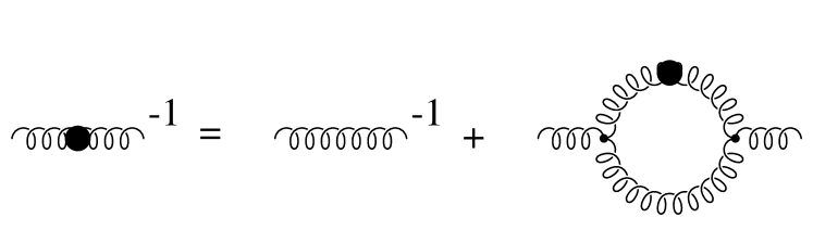
Figure 1: Diagrammatic representation of the gluon Dyson–Schwinger equation in Mandelstam’s approximation.

The form for the three–gluon vertex is motivated by its Slavnov-Taylor identity, which neglecting all ghost contributions in the covariant gauge reads:

$$p^{\mu}\Gamma^{\mu\nu\rho}(p,q,k)=\frac{k^{2}}{Z(k^{2})}\left(\delta^{\nu\rho}-\frac{k^{\nu}k^{\rho}}{k^{2}}\right)-\frac{q^{2}}{Z(q^{2})}\left(\delta^{\nu\rho}-\frac{q^{\nu}q^{\rho}}{q^{2}}\right)\quad,$$ (2)

where $p,q$ and $k$ are incoming momenta and $Z(k^{2})$ is the invariant function of the dressed gluon propagator,

$$D^{\mu\nu}(k^{2})=\frac{Z(k^{2})}{k^{2}}\left(\delta^{\mu\nu}-\frac{k^{\mu}k^{\nu}}{k^{2}}\right)+\xi\frac{k^{\mu}k^{\nu}}{k^{4}}\quad.$$ (3)

The Slavnov–Taylor identity fixes the longitudinal part of the vertex. It can be derived along the general procedure of ref. [8]. In the simple version of Eq. (2) without ghost contributions the solution is:

$$\Gamma_{L}^{\mu\nu\rho}(p,q,k)=A_{+}(p^{2},q^{2})\delta^{\mu\nu}(p-q)^{\rho}+A_{-}(p^{2},q^{2})\delta^{\mu\nu}(p+q)^{\rho}\\ +C(p^{2},q^{2})(\delta^{\mu\nu}pq-p^{\nu}q^{\mu})(p-q)^{\rho}+\text{cycl. permut.},$$ (4)

with

$$A_{\pm}(p^{2},q^{2})=\frac{1}{2}\left(\frac{1}{Z(p^{2})}\pm\frac{1}{Z(q^{2})}\right)\quad\text{and}\quad C(p^{2},q^{2})=2\frac{A_{-}(p^{2},q^{2})}{p^{2}-q^{2}}\;.$$ (5)

Assuming that $Z(q^{2})$ is a slowly varying function one may write

$$\Gamma_{L}^{\mu\nu\rho}(p,q,k)=A_{+}(p^{2},q^{2})\Gamma_{0}^{\mu\nu\rho}(p,q,k)\;.$$ (6)

While this form for the full three–gluon vertex simplifies equation (1) even more than the use of another bare vertex, $\Gamma=\Gamma_{0}$, it is regarded superior to the latter since it accounts for some of the dressing of the vertex as it results from the Slavnov–Taylor identity. With $\Gamma=\Gamma_{L}$ from (6) the Dyson–Schwinger equation can now be cast in the simple form

$${D^{-1}}^{\mu\nu}(k) = {D_{0}^{-1}}^{\mu\nu}(k)\,+\,\frac{g_{0}^{2}N_{C}}{32\pi^{4}}\int\!d^{4}\!q\>\Gamma_{0}^{\mu\rho\alpha}(k,q-k,-q)$$ (7)

$$\hskip-19.91684pt\times D^{\alpha\beta}(q)D_{0}^{\rho\sigma}(k-q)\Gamma_{0}^{\beta\sigma\nu}(q,k-q,-k)\quad.$$

This equation is schematically depicted in Fig. 1. In solving it an additional condition is implemented in the Mandelstam approximation. Eq. (2) and its solution (4,5) for $p^{2}\to 0$ entail that

$$\lim_{k^{2}\to 0}\frac{k^{2}}{Z(k^{2})}=0,\qquad\text{or}\qquad\lim_{k^{2}\to 0}D_{\!\mu\nu}^{-1}(k^{2})=0\quad.$$ (8)

While imposing this additional condition seems consistent with the other assumptions in the Mandelstam approximation, it has to be emphasized that concluding (8) as a result of (2) relies on neglecting all ghost contributions in covariant gauges. In fact, if ghosts are included in resolving the Slavnov–Taylor identity for the 3–gluon vertex, condition (8) has to be modified [4].

In a manifestly gauge invariant formulation the Dyson–Schwinger equation for the inverse gluon propagator in the covariant gauge would be transverse without further adjustments. The longitudinal part of the gluon propagator does not acquire dressing and cancels with the one of the bare propagator. This may be violated due to the neglect of ghosts, the violation of Slavnov–Taylor identities and also due to a regularization that does not preserve the residual local invariance, i.e., the invariance under transformations generated by harmonic gauge functions ($\partial^{2}\Phi(x)=0$). The latter is the case for an $O(4)$ invariant Euclidean cutoff $\Lambda$, which we will use to regularize Eq. (7). In the present approximation, longitudinal terms can be eliminated by contracting Eq. (7) with the transversal projector,

$$P^{\mu\nu}(k)=\delta^{\mu\nu}-\frac{k^{\mu}k^{\nu}}{k^{2}}\;.$$ (9)

After performing the angular integrations the equation for the gluon renormalization function $Z(k^{2})$ in Landau gauge ($\xi=0$) then becomes [1]

$$\frac{1}{Z(k^{2})}=1+\frac{g_{0}^{2}}{16\pi^{2}}\int_{0}^{k^{2}}\frac{dq^{2}}{k^{2}}\left(\frac{7}{8}\frac{q^{4}}{k^{4}}-\frac{25}{4}\frac{q^{2}}{k^{2}}-\frac{9}{2}\right)Z(q^{2})\\ +\frac{g_{0}^{2}}{16\pi^{2}}\int_{k^{2}}^{\Lambda^{2}}\frac{dq^{2}}{k^{2}}\left(\frac{7}{8}\frac{k^{4}}{q^{4}}-\frac{25}{4}\frac{k^{2}}{q^{2}}-\frac{9}{2}\right)Z(q^{2})\;.$$ (10)

However, the above equation contains a quadratically ultraviolet divergent term. This term violates the masslessness condition (8) and has therefore been dismissed. As observed by Brown and Pennington [7], in general, quadratic ultraviolet divergences can occur only in the part of the inverse gluon propagator proportional to $\delta^{\mu\nu}$. Therefore, that part cannot be unambiguously determined, it depends on the routing of the momenta. This is due to the various violations of gauge invariance mentioned above. The unambiguous term proportional to $k^{\mu}k^{\nu}$ can be obtained by contracting (7) with

$$R^{\mu\nu}(k)=\delta^{\mu\nu}-4\frac{k^{\mu}k^{\nu}}{k^{2}}\quad.$$ (11)

In this case, upon angle integration instead of (10) one obtains [7]

$$\frac{1}{Z(k^{2})}=1+\frac{g_{0}^{2}}{16\pi^{2}}\int_{0}^{k^{2}}\frac{dq^{2}}{k^{2}}\left(\frac{7}{2}\frac{q^{4}}{k^{4}}-\frac{17}{2}\frac{q^{2}}{k^{2}}-\frac{9}{8}\right)Z(q^{2})\\ +\frac{g_{0}^{2}}{16\pi^{2}}\int_{k^{2}}^{\Lambda^{2}}\frac{dq^{2}}{k^{2}}\left(\frac{7}{8}\frac{k^{4}}{q^{4}}-7\frac{k^{2}}{q^{2}}\right)Z(q^{2}).$$ (12)

It is clear that the assumptions made so far are drastic, and it is questionable how much of the original theory survived.Furthermore, inclusion of ghosts changes the conclusions on the infrared behavior of gluon propagator and the running coupling even qualitatively [4]. For the sake of a detailed understanding of what exactly can be attributed to ghosts, it is nevertheless necessary to thoroughly study the implications of the Mandelstam approximation, most remarkably on the running coupling, in order to compare to conclusions of the present and earlier work on the Dyson–Schwinger equations of Landau gauge QCD. Besides this, the major numerical concepts used in the present paper, entirely devoted to the Mandelstam approximation, will apply to the coupled system of ghosts and gluons in Landau gauge with little changes.

One might think that the particular problem problem with ghosts can be avoided using gauges such as the axial gauge, in which there are no ghosts in the first place. As for studies of the gluon Dyson–Schwinger equation in axial gauge [9, 10, 11] it is important to note that these rely on an ad hoc assumption on the tensor structure of the gluon propagator. The occurrence of a second independently possible term, which happens to vanish in perturbation theory, has been disregarded so far [12]. In fact, if the complete tensor structure of the gluon propagator in axial gauge is taken into account properly, one arrives at a coupled system of equations which is of similar complexity as the ghost–gluon system in the Landau gauge [13]. Progress is desirable in axial gauge as well, of course. A necessary prerequisite for this, however, is a proper treatment of the spurious infrared divergences which are well known to be present in axial gauge due to zero modes. This can be achieved by either introducing redundant degrees of freedom, i.e. ghosts, also in this gauge (by which it obviously looses its particular advantage) or by using a modified axial gauge [14], which is specially designed to account for those zero modes. Eventually, progress in more than one gauge will be the only reliable way to asses the influence of spurious gauge dependencies.

1.3 Renormalization

The logarithmic ultraviolet divergences in equations (10) and (12) can be removed by multiplicative renormalization. Introducing the renormalized gluon propagator $D_{R}$ and the renormalized coupling $g$ the renormalization constants $Z_{3}$ and $Z_{g}$ are defined by $D=Z_{3}D_{R}$ and $g_{0}=Z_{g}g$ respectively. From the Dyson–Schwinger equation for the gluon propagator in Mandelstam approximation (7), renormalized this way, we obtain

$$Z_{R}(k^{2})=\left[Z_{3}+Z_{3}^{2}Z_{g}^{2}\,\frac{g^{2}}{16\pi^{2}}\,I_{Z_{R}}(k^{2})\right]^{-1}\;.$$ (13)

Here, $I_{Z_{R}}:=I[Z_{R}]$ is a functional of $Z_{R}(k^{2})$; for Eq. (12) $I_{Z_{R}}(k^{2})$ is given by

$$I_{Z_{R}}(k^{2})=\frac{1}{k^{2}}\int_{0}^{k^{2}}dq^{2}\left(\frac{7}{2}\frac{q^{4}}{k^{4}}-\frac{17}{2}\frac{q^{2}}{k^{2}}-\frac{9}{8}\right)Z_{R}(q^{2})\\ +\frac{1}{k^{2}}\int_{k^{2}}^{\Lambda^{2}}dq^{2}\left(\frac{7}{8}\frac{k^{4}}{q^{4}}-7\frac{k^{2}}{q^{2}}\right)Z_{R}(q^{2})\;.$$ (14)

An analogous form follows for Mandelstam’s original equation. After the subtraction of the ultraviolet divergences, we use the limit $\Lambda\to\infty$ for the cutoff $\Lambda$ implicitly. Confessing that we are dealing with renormalized quantities in the following, we dismiss the subscript $R$ again. Below we will prove the identity $Z_{g}Z_{3}=1$ for the Mandelstam approximation. Furthermore, we adopt a momentum subtraction scheme requiring the gluon self–energy to vanish at the renormalization point $\mu$, i.e.,

$$Z(\mu^{2})=1\qquad\Rightarrow\qquad Z_{3}=1-\frac{g^{2}}{(4\pi)^{2}}\,I_{Z}(\mu^{2})\;.$$ (15)

With this and $\alpha_{S}(\mu^{2})=g^{2}(\mu^{2})/4\pi$ Eq. (13) reads,

$$Z(k^{2})=\left[1+\frac{\alpha_{S}(\mu^{2})}{4\pi}\left[I_{Z}(k^{2})-I_{Z}(\mu^{2})\right]\right]^{-1}\;.$$ (16)

To determine the behavior of $Z(k^{2})$ for $k^{2}\to 0$ we first notice that

1. for a constant $Z(k^{2})$ the last term in (14) yields an infrared logarithm. Therefore, a solution to (16) cannot approach a constant as $k^{2}\to 0$. Any constant term in the denominator on the r.h.s. of (16) has to vanish. This is a first constraint for a possible solution.

2. Similarly $Z(k^{2})\sim k^{2}$ as $k^{2}\to 0$ is inconsistent since then the next to leading term yields a logarithmic contribution.

3. Now let us assume $Z(k^{2})\sim 1/k^{2}$. This form yields exclusively terms that violate the condition (8). Such terms have to be subtracted. Since the kernels of all integrals are linear in $Z$, this is achieved by simply subtracting a corresponding contribution from $Z$ in the integrands. Thus defining $F(k^{2})$ by

   $$Z(k^{2})=\frac{b}{k^{2}}+F(k^{2})$$ (17)

   with some constant $b$, we further explore Ansätze for $F$, which is the remainder of $Z$ in the integrals.

To isolate the infrared singular term $b/k^{2}$ we rewrite equation (16) as:

$$Z(k^{2})=\frac{b}{k^{2}}+F(k^{2})=\frac{1}{A+Bk^{2}+J(k^{2})}\;,$$ (18)

where

$$A =1-\frac{\alpha_{S}(\mu^{2})}{4\pi}\left[7\int_{0}^{\Lambda^{2}}dq^{2}\>\frac{F(q^{2})}{q^{2}}+I_{F}(\mu^{2})\right],$$ (19)

$$B =\frac{7}{8}\frac{\alpha_{S}(\mu^{2})}{4\pi}\int_{0}^{\infty}dq^{2}\>\frac{F(q^{2})}{q^{4}}\;,$$ (20)

$$J(k^{2}) =\frac{\alpha_{S}(\mu^{2})}{4\pi}\int_{0}^{k^{2}}dq^{2}\biggl{(}\frac{7}{2}\frac{q^{4}}{k^{6}}-\frac{17}{2}\frac{q^{2}}{k^{4}}-\frac{9}{8}\frac{1}{k^{2}}+7\frac{1}{q^{2}}-\frac{7}{8}\frac{k^{2}}{q^{4}}\biggr{)}F(q^{2})\;.$$ (21)

As already stated in (1) above, a possible solution will have to obey $A=0$. We will verify below that $A=0$ is not an independent constraint but an identity. In addition, we see that $b=1/B$ must be met, which will be imposed as a constraint on a possible solution.

Introducing dimensionless variables and appropriately scaled gluon self–energy functions $\tilde{Z}$ and $\tilde{F}$ by

$$x=\frac{k^{2}}{b}\sqrt{\frac{4\pi}{\alpha_{S}(\mu^{2})}}=:\frac{k^{2}}{\lambda^{2}}\quad\hbox{and}\quad\tilde{Z}(x)=\sqrt{\frac{\alpha_{S}(\mu^{2})}{4\pi}}\,Z(k^{2})=\frac{1}{x}+\tilde{F}(x)\;,$$ (22)

the equation under consideration can be rendered dimensionless and scale–independent. From equation (18) we obtain

$$\frac{x}{1+x\tilde{F}(x)}=\tilde{A}+\tilde{B}x+\int_{0}^{x}\frac{dy}{x}\left(\frac{7}{2}\frac{y^{2}}{x^{2}}-\frac{17}{2}\frac{y}{x}-\frac{9}{8}+7\frac{x}{y}-\frac{7}{8}\frac{x^{2}}{y^{2}}\right)\tilde{F}(y)\;.$$ (23)

Here,

$$\tilde{B}=bB=\frac{7}{8}\int_{0}^{\infty}dy\>\frac{\tilde{F}(y)}{y^{2}}\stackrel{{\scriptstyle!}}{{=}}1\;,$$ (24)

from the constraint mentioned above. Since $\tilde{F}(x)$ vanishes for $x\to 0$ as will be shown later, in this limit equation (23) shows explicitly that the $x$-independent constant

$$\tilde{A}=\frac{4\pi}{g}A=0\;.$$ (25)

With (24) equation (23) therefore yields

$$\frac{x^{2}\tilde{F}(x)}{1+x\tilde{F}(x)}=-\int_{0}^{x}\frac{dy}{x}\left(\frac{7}{2}\frac{y^{2}}{x^{2}}-\frac{17}{2}\frac{y}{x}-\frac{9}{8}+7\frac{x}{y}-\frac{7}{8}\frac{x^{2}}{y^{2}}\right)\tilde{F}(y)\;.$$ (26)

Before we turn to the numerical solution of (26) with the constraint (24), some remarks need to be made.

First note that the renormalization condition $Z(\mu^{2})=1$ implies that

$$\tilde{\alpha}_{S}(s)=4\pi\,\tilde{Z}^{2}(s)\;,$$ (27)

with $s:=\mu^{2}/\lambda^{2}$ and $\tilde{\alpha}_{S}(s):=\alpha_{S}(\mu^{2})$. This is compatible with the definition of $\tilde{A}$ which yields ($L:=\Lambda^{2}/\lambda^{2}$)

$$\tilde{\alpha}_{S}(s) =4\pi\left[\tilde{A}+7\int_{0}^{L}\!dy\>\frac{\tilde{F}(y)}{y}+I_{\tilde{F}}(s)\right]^{-2}$$ (28)

$$=4\pi\biggl{[}\tilde{A}+\tilde{B}s+\frac{1}{s}\int_{0}^{s}\!dy\left(\frac{7}{2}\frac{y^{2}}{s^{2}}-\frac{17}{2}\frac{y}{s}-\frac{9}{8}+7\frac{s}{y}-\frac{7}{8}\frac{s^{2}}{y^{2}}\right)\tilde{F}(y)\biggr{]}^{-2}\!.$$

The right hand side above is identical to the one of (23) with $x\leftrightarrow s$, and thus (28) to (27). The fact that only $\tilde{A}=0$ is consistent, i.e., the infrared behavior of the solution, entails that the running coupling is singular in the infrared.

Furthermore, we observe that a solution to the system of equations (26) and (24) is a renormalization group invariant function. The argument for this is as follows: Assume that the product $gD_{\mu\nu}(k)$ does not acquire multiplicative renormalization. This means that $\tilde{Z}\propto gZ$ is a renormalization group invariant combination. For solutions of the form as given in (18) we conclude that $\sqrt{\alpha_{S}/(4\pi)}b=:\lambda^{2}$ is a renormalization group invariant of mass dimension two. Therefore, the introduction of the dimensionless variable $x=k^{2}/\lambda^{2}$ in (22) does not introduce an implicit dependence on the renormalization scale $\mu$ in the explicitly scale–independent set of equations (26,24). This verifies the assumption, i.e., a solution $\tilde{Z}(x)=gZ(k^{2})/(4\pi)$ of (26,24) is a renormalization group invariant. For the renormalization constants this entails that $Z_{g}Z_{3}=1$ in the Mandelstam approximation. This is to be compared to the Abelian approximation to QCD, in which $Z_{g}Z_{3}^{1/2}=1$ or, equivalently, $g^{2}D_{\mu\nu}(k)$ is a renormalization group invariant combination (one application of this is ref. [15]). Closer to the present case is the renormalization group improved one–loop result in QCD. In perturbative QCD the power $\delta$ of the coupling in the invariant combination $g^{\delta}D_{\mu\nu}(k)$ depends on the number of quark–flavors $N_{f}$. Two examples are $\delta=13/11$ for $N_{f}=0$ and $\delta=1$ for $N_{f}=3$. Even though $N_{f}=0$ in Mandelstam approximation, it resembles the three flavor result at this point. However, in contrast to perturbation theory the identity $Z_{g}Z_{3}=1(\delta=1)$ holds for all momentum scales $\mu$ in Mandelstam approximation.

We conclude the discussion of the renormalization with a comment on the choice of the non–perturbative subtraction scheme (15). Since $gZ(k^{2})$ is a dimensionless renormalization group invariant in Mandelstam approximation, it is a function of the running coupling $\bar{g}(t,g)$,

$$gZ(k^{2})=f(\bar{g}(t_{k},g))\;,\quad t_{k}=\frac{1}{2}\ln k^{2}/\mu^{2}\;.$$ (29)

Asymptotically, the momentum subtraction scheme is defined by $f(x)\to x$ for $x\to 0$. If the product $gZ(k^{2})$ is to have a physical meaning, e.g., as potential between static color sources, it should be independent under changes $(g,\mu)\to(g^{\prime},\mu^{\prime})$ according to the renormalization group. Taken the idea of renormalization group invariance literally for arbitrary scales $\mu^{\prime}$,

$$gZ({\mu^{\prime}}^{2})\stackrel{{\scriptstyle!}}{{=}}g^{\prime}=\bar{g}(\ln(\mu^{\prime}/\mu),g)\;.$$ (30)

Then, $f(x)\equiv x$, $\forall x$, and, accordingly, $Z(\mu^{2})=1$, $\forall\mu$. This is the only physically sensible non–perturbative extension of the momentum subtraction scheme in the present context. Note that (29) with $f(x)\equiv x$ is identical to (27) with $s\leftrightarrow x$, the renormalization scheme is thus equivalent to defining the non–perturbative running coupling by the product of the coupling constant and the gluon renormalization function in the Mandelstam approximation.

2 Numerical methods

2.1 Series expansion in the infrared and asymptotic behavior in the ultraviolett

A straightforward implementation of (26) fails due to delicate cancelations in the infrared. Therefore the expansion in the the infrared has to be pushed beyond leading order for $\tilde{Z}(x)$. Making the Ansatz $\tilde{F}(x)=ax^{\gamma}$ one sees that no solution exists for $\gamma\leq 1$. For $\gamma>1$ eqn. (26) yields

$$x^{2+\gamma}=-C_{00}(\gamma)x^{\gamma}-aC_{00}(\gamma)x^{1+2\gamma}$$ (31)

with

$$C_{00}(\gamma)=\frac{7}{2(\gamma+3)}-\frac{17}{2(\gamma+2)}-\frac{9}{8(\gamma+1)}+\frac{7}{\gamma}-\frac{7}{8(\gamma-1)}\quad.$$ (32)

Obviously the coefficient $C_{00}(\gamma)$ has to vanish in order to permit a selfconsistent solution. This yields a cubic equation with a unique solution for $\gamma>1$:

$$\gamma_{0}=\frac{2}{9}\sqrt{229}\cos\left(\frac{1}{3}\arccos\left(-\frac{1099}{229\sqrt{229}}\right)\right)-\frac{13}{9}\approx 1.2705\quad.$$ (33)

An analogous condition was already found by Mandelstam for his original equation [1]. It is interesting to note that the value of $\gamma_{0}$ given here is numerically very close to the one obtained by Mandelstam ($\gamma_{0}=\sqrt{\frac{31}{6}}-1\approx 1.273$), even though the coefficients in (12) and in (10) are completely different.

Looking at the corresponding results given in [3] one observes that their infrared leading terms for $F(k^{2})$ do not obey the constraint (33) for $\gamma_{0}$. We verified numerically that the expressions given in ref. [3] reproduce themselves under the integral equation in the momentum range given in the corresponding figure in this reference (Fig. 3 in [3]). However, trying to extend the numerical calculations further to the infrared along the lines of [3] we observed that $Z(k^{2})$ became singular at lower but finite $k^{2}$. Due to this fact an iterative numerical solution proved impossible without constraining the infrared behavior of $Z(k^{2})$ to that according to the discussion of the solution given above. Therefore, we conclude that while the expressions for $Z(k^{2})$ in [3] with the parameters given there are a numerical approximation to the solution of Eq. (16), they do not represent the exact analytic result particularly for $k^{2}\ll\Lambda_{QCD}^{2}$.

For the numerical solution of Eq. (26) it turns out to be necessary to study the subleading infrared behaviour of $\tilde{F}(x)$ in more detail. This is possible by an asymptotic expansion of $\tilde{F}(x)$ at small $x$ analogous to what was introduced by Atkinson et al. for Mandelstam’s original equation in ref. [2],

$$\tilde{F}(x)=\sum_{m=0}^{M}\sum_{n=0}^{N}\>a_{mn}\,x^{\gamma_{0}+n\gamma_{0}+n+2m}\quad.$$ (34)

The coefficients $a_{mn}$ can be determined from Eq. (26):

$$a_{0n} =0\qquad\qquad\text{for $n>0$}$$ (35)

$$a_{m0} =\frac{a_{m-1,0}}{C_{m0}}\qquad\text{for $m>0$}$$

$$a_{mn} =\frac{1}{C_{mn}}\biggl{(}a_{m-1,n}-\sum_{m^{\prime}=0}^{m-1}\sum_{n^{\prime}=0}^{n-1}\>a_{m^{\prime}n^{\prime}}a_{m-m^{\prime},n-n^{\prime}}C_{m-m^{\prime},n-n^{\prime}}\biggr{)}\,,\;m,n>0$$

with the matrix $C_{mn}$ given by

$$C_{mn}= -\frac{7}{2(\gamma_{0}+n\gamma_{0}+n+2m+3)}+\frac{17}{2(\gamma_{0}+n\gamma_{0}+n+2m+2)}$$

$$+\frac{9}{8(\gamma_{0}+n\gamma_{0}+n+2m+1)}-\frac{7}{\gamma_{0}+n\gamma_{0}+n+2m}$$

$$+\frac{7}{8(\gamma_{0}+n\gamma_{0}+n+2m-1)}\quad.$$ (36)

The double series (34) is thus fixed up to the coefficient $a_{00}$ of the infrared leading term. With this at hand the infrared region up to a matching point $x_{0}$ is treated analytically and the equation for $\tilde{F}(x)$ becomes:

$$\frac{x^{2}\tilde{F}(x)}{1+x\tilde{F}(x)}=\sum_{m=0}^{M}\sum_{n=0}^{N}\Biggl{[}-\frac{7}{2(\gamma_{0}+n\gamma_{0}+n+2m+3)}\left(\frac{x_{0}}{x}\right)^{3}\\ +\frac{17}{2(\gamma_{0}+n\gamma_{0}+n+2m+2)}\left(\frac{x_{0}}{x}\right)^{2}+\frac{9}{8(\gamma_{0}+n\gamma_{0}+n+2m+1)}\left(\frac{x_{0}}{x}\right)\\ -\frac{7}{\gamma_{0}+n\gamma_{0}+n+2m}+\frac{7}{8(\gamma_{0}+n\gamma_{0}+n+2m-1)}\left(\frac{x_{0}}{x}\right)^{-1}\Biggr{]}a_{mn}x_{0}^{\gamma_{0}+n\gamma_{0}+n+2m}\\ -\int_{x_{0}}^{x}\frac{dy}{y}\left(\frac{7}{2}\frac{y^{3}}{x^{3}}-\frac{17}{2}\frac{y^{2}}{x^{2}}-\frac{9}{8}\frac{y}{x}+7-\frac{7}{8}\frac{x}{y}\right)\tilde{F}(y)\quad.$$ (37)

Similarly the infrared part of the constraint (24) is rewritten with the help of the asymptotic series. In the numerical evaluation of the (ultraviolet finite) integral in Eq. (24) large momentum contributions are also truncated. Though the resulting error becomes negligible for a sufficiently large ultraviolet cutoff $x_{1}$, convergence is improved by correcting this error analytically. This is possible because $\tilde{F}(x)$ can be replaced by its leading perturbative from for $x>x_{1}$ and sufficiently large $x_{1}$, which allows to calculate the finite correction term for the integration from $x_{1}$ to infinity on the r.h.s. of Eq. (24) analytically. To obtain this ultraviolet behaviour, the l.h.s. of eqn. (26) is expanded for $x\tilde{F}(x)\rightarrow\infty$. The leading terms cancel each other due to the constraint (24). The next to leading order terms upon differentiation yield the differential equation

$$x\tilde{F}^{\prime}(x)=-7\tilde{F}^{3}(x)\;,$$ (38)

which is solved by

$$\tilde{F}(x)=\frac{1}{\sqrt{14\ln x}}\quad\text{for}\quad x\rightarrow\infty\;.$$ (39)

Going to higher orders one starts by expanding (26), neglecting terms of order $1/x$ and higher and making use of Eq. (24). Substituting $t=\sqrt{\ln x}$ one arrives at

$$\frac{d}{dt}\frac{1}{\tilde{F}(t)}=\sqrt{14}+\frac{dg(t)}{dt}=\frac{14\,t}{\sqrt{14}\,t+g(t)}+\frac{10}{3\sqrt{14}}\frac{1}{t^{2}}+\ldots\;,$$ (40)

where we defined the function $g(t)$ for convenience. Thus

$$\frac{dg(t)}{dt}=-\frac{g(t)}{t}+\frac{10}{3\sqrt{14}}\,\frac{1}{t^{2}}+\mathcal{O}\left(\frac{g^{2}(t)}{t^{2}}\right)$$ (41)

which is solved by

$$g(t)=-\frac{c\sqrt{14}}{t}+\frac{10}{3\sqrt{14}}\,\frac{\ln t}{t}+\mathcal{O}\left(\frac{1}{t^{4}}\right)+\mathcal{O}\left(\frac{1}{\text{e}^{x^{2}}}\right)\;.$$ (42)

Resubstituting for $x$ finally gives

$$\tilde{F}(x)=\frac{1}{\sqrt{\kappa_{0}\ln x}}-\frac{(\kappa_{1}/\kappa_{0})\ln\ln x-\kappa_{0}c}{(\kappa_{0}\ln x)^{3/2}}+\mathcal{O}\left(\frac{1}{(\ln x)^{5/2}}\right)+\mathcal{O}\left(\frac{1}{x}\right)\;,$$ (43)

where $\kappa_{0}=14$ and $\kappa_{1}=70/3$. The integration constant $c$ is difficult to determine numerically because of the unknown contribution of the terms neglected and the extremely large scales necessary for the leading logarithms to dominate. We find roughly that $c\approx 1$, its exact value is irrelevant, however. With $x=k^{2}/\lambda^{2}$ and $\tilde{Z}(x)=gZ(k^{2})/(4\pi)$ the leading term in (43) is equivalent to

$$Z(k^{2})\to\frac{1}{\sqrt{\kappa_{0}/(4\pi)^{2}\,g^{2}\ln(k^{2}/\lambda^{2})}}\qquad\text{for $k^{2}\to\infty$}\;.$$ (44)

This resembles the renormalization group improved perturbative result,

$$Z_{pt}(k^{2})=\left(\beta_{0}\,g^{2}\ln k^{2}/\Lambda^{2}\right)^{-\delta/2}\quad,$$ (45)

and allows for the following identifications:

• The Callan–Symanzik coefficient $\beta_{0}$ is given by $\beta_{0}=\kappa_{0}/(4\pi)^{2}$, and the above value for $\kappa_{0}$ has to be compared to its perturbative result $\kappa_{0}=11-(2/3)N_{f}$.

• Since we use a momentum subtraction scheme, we identify the QCD scale to be used as $\Lambda_{\text{MOM}}=\lambda$.

• The anomalous dimension of the gluon field $\gamma_{A}(g)$ in perturbation theory is given by $\gamma_{A}(g)=\gamma_{A}^{0}g^{2}$ with $\gamma_{A}^{0}=(13/2-(2/3)N_{f})/(4\pi)^{2}$, and the exponent in the r.h.s. of (45) is $\delta/2=\gamma_{A}^{0}/\beta_{0}$. The fact that $\delta=1$ for the asymptotic behavior in the Mandelstam approximation confirms that $Z_{g}Z_{3}=1$, which is equivalent to $\gamma_{A}^{0}=\beta_{0}/2$. We thus obtain $\gamma_{A}^{0}=7/(4\pi)^{2}$.

The values for the scaling coefficients $\beta_{0}$ and $\gamma_{A}^{0}$ obtained from the Mandelstam approximation are reasonably close to their perturbative values for $N_{f}=0$. The respective values for Mandelstam’s original equation (10) are $\beta_{0}=(25/2)/(4\pi)^{2}$ and $\gamma_{A}^{0}=(25/4)/(4\pi)^{2}$.

With the asymptotic infrared as well as ultraviolet contributions integrated analytically, the constraint (24) can now be written,

$$1=\frac{7}{8}\Biggl{[}\sum_{m=0}^{M}\sum_{n=0}^{N}a_{mn}\frac{x_{0}^{\gamma_{0}+n\gamma_{0}+n+2m-1}}{\gamma_{0}+n\gamma_{0}+n+2m-1}\\ +\int_{x_{0}}^{x_{1}}dy\frac{\tilde{F}(y)}{y^{2}}+\sqrt{\frac{\pi}{14}}\operatorname{erfc}\sqrt{\ln x_{1}}\Biggr{]}\;.$$ (46)

The integrals in eqn. (37) and (46) are calculated with a Simpson integration routine of fourth order. The meshpoints have been chosen equidistant on a logarithmic scale, i.e. we have substituted

$$\int dy\longrightarrow\int du\,y\quad\text{with}\quad u=\ln y\quad.$$ (47)

Note that choosing an equidistant mesh in $y$ will not result in a convergent iterative process.

Equation (37) can now be solved iteratively. Starting with a trial function for $\tilde{F}(x)$ the r.h.s. of (37) is evaluated and, in order to account for the constraint, the result is rescaled appropriately before it is used in the next iteration. To leading order the contribution from the infrared expansion is proportional to $a_{00}$. It is therefore sufficient to rescale $a_{00}$ linearly. This way, the coefficient $a_{00}$ is determined numerically from the iteration process. For Eq. (12) we obtain $a_{00}=0.29446...$, and for (10) its value is $a_{00}=0.29421...$. The infrared matching point $x_{0}$ is chosen in a region around $0.2$. For this value it proves sufficient to truncate the series (34) at $M=N=4$ (see Fig. 2). For lower orders of the series we observe small bumps at the matching point. Changing the matching point in a regime from 0.15 to 0.25 has no influence on the numerical solution. The lower limit is dictated by convergence of the iterative process; the upper limit by a reasonable accuracy of the asymptotic series.

Using the numerical solution for $Z$, see Eq. (12), the renormalization group invariant product $gZ$ as a function of $k^{2}/\Lambda_{\text{MOM}}^{2}$ is shown in Fig. 3. The solution to Mandelstam’s original equation (10) is almost indistinguishable on this scale.

Figure 2: The numerical solution $\tilde{F}(x)$ together with several asymptotic series of different order.

Figure 3: The numerical solution $\tilde{F}(x)$ and for comparison $\tilde{Z}(x)=1/x+\tilde{F}(x)$.

2.2 The running strong coupling

With the solution $\tilde{Z}(x)$ the running coupling $\alpha_{S}(\mu^{2})=\tilde{\alpha}_{S}(s)$ with $s=\mu^{2}/\Lambda_{\text{MOM}}^{2}$ follows for the subtraction scheme (15) from Eq. (27). The result together with its analytically extracted asymptotic forms is shown in the left graph of Fig. 4. In the infrared we have,

$$\tilde{\alpha}_{S}(s)\to 4\pi\frac{1}{s^{2}}\quad\text{or}\quad g(\mu^{2})\to 4\pi\frac{\Lambda_{\text{MOM}}^{2}}{\mu^{2}}\quad\text{for $\mu^{2}\to 0$ .}$$ (48)

In the ultraviolet one obtains from Eq. (43) the leading logarithmic behavior,

$$\alpha_{S}(\mu^{2})=\tilde{\alpha}_{S}(s)=\frac{4\pi}{\kappa_{0}\ln s}\left(1-\frac{2\kappa_{1}}{\kappa_{0}^{2}}\frac{\ln\ln s}{\ln s}+\frac{2c}{\ln s}\right)+\mathcal{O}\left(\frac{1}{(\ln s)^{3}}\right)+\mathcal{O}\left(\frac{1}{s}\right)\;.$$ (49)

This form resembles the two–loop perturbative result if the integration constant $c$ is set to zero. The value of $\kappa_{1}=70/3$ compares to $\kappa_{1}=51-(19/3)N_{f}$ in perturbation theory [16]. The Callan–Symanzik $\beta$ function, $\beta(g)=\mu(dg/d\mu)$, follows readily for all positive values of the coupling. The numerical result is shown in the right graph of Fig. 4. Its limits are

$$\beta(g)\to-\beta_{0}g^{3}\quad\text{for}\quad g\to 0\quad\text{and}\quad\beta(g)\to-2g\quad\text{for}\quad g\to\infty\;.$$ (50)

An alternative way to obtain the $\beta$ function follows directly from the coupling renormalization $g_{0}=Z_{g}g$. Because of $Z_{g}Z_{3}=1$ the gluon field renormalization (15) is equivalent to a renormalization condition that relates the $\mu$–independent bare coupling to the renormalized one,

$$\frac{4\pi}{g_{0}}=4\pi\frac{Z_{3}}{g}=\frac{4\pi}{g}-I_{\tilde{Z}}(\mu^{2})\;.$$ (51)

This determines the $\beta$ function of the Mandelstam approximation with a momentum subtraction scheme (fixing $Z(\mu^{2})$ to a $\mu$ independent constant as in (15)). Since $Z_{g}Z_{3}=1$ the anomalous dimension of the gluon $\gamma_{A}(g)$ is,

$$\gamma_{A}(g)=-\frac{1}{2}\frac{\mu}{Z_{3}}\frac{dZ_{3}}{d\mu}=-\frac{\beta(g)}{2g}\;.$$ (52)

From the infrared behavior of the renormalization group invariant product $gD_{\mu\nu}(k)$ we may deduce a linear rising potential between static color sources for large distances. This allows us to relate the coefficient of the $1/k^{4}$ term in the interaction to the string tension $\sigma$,

$$\frac{gZ(k^{2})}{k^{2}}\to 8\pi\frac{\sigma}{k^{4}}\quad\text{for}\quad k^{2}\to 0\;.$$ (53)

With the identification $\Lambda_{\text{MOM}}^{2}=\lambda^{2}$ (from the ultraviolet) and the infrared behavior of the solution,

$$gZ(k^{2})\to 4\pi\frac{\lambda^{2}}{k^{2}}\;,$$ (54)

the non–perturbative result for the gluon propagator relates the string tension to the scale $\Lambda_{\text{MOM}}$, yielding

$$2\sigma=\Lambda_{\text{MOM}}^{2}$$ (55)

in the Mandelstam approximation. The string tension can be fixed from quarkonia potentials and Regge phenomenology [17, 18]. The result is a value of about $\sigma=0.18\text{GeV}^{2}$. This has also been confirmed in lattice calculations [19]. Here, it corresponds to a scale $\Lambda_{\text{MOM}}$ of 600 MeV.

Figure 4: The strong coupling $\alpha_{S}(\mu^{2})$ with $\mu^{2}$ in units of the QCD scale $\Lambda_{\text{MOM}}^{2}$ and its asymptotic forms according to (48) and (49) with $c=1$ (left); and the non–perturbative $\beta$ function of the Mandelstam approximation (right).

3 Conclusions

In this paper we have derived the infrared behavior of the strong coupling constant from Mandelstam’s approximation [1] to the gluon Dyson–Schwinger equation. This approximation results in a gluon propagator diverging like $\sigma/k^{4}$ for $k^{2}\to 0$. This highly infrared singular behavior of the gluon propagator generates a linearly rising potential between static color sources. The corresponding string tension $\sigma$ can be used to fix the scale in the resulting gluon self–energy. In particular, the non–perturbative solution allows to relate the string tension to the QCD scale $\Lambda_{\text{MOM}}$. This relation is in reasonable agreement with the phenomenological values of the respective physical constants. Note that dimensional transmutation occurs here: The coefficient $\lambda^{2}=2\sigma$ of the infrared singular term is a dimensionful physical quantity, whereas all input is dimensionless except for the renormalization scale $\mu$.

We have shown that the product of the coupling and the gluon propagator, $gD_{\mu\nu}(k)$, does not acquire multiplicative renormalization in Mandelstam approximation ($Z_{g}Z_{3}=1$). We calculated the gluon self–energy in a renormalization group invariant fashion. Besides the running coupling $\alpha_{S}(\mu^{2})$ we obtained the non–perturbative Callan–Symanzik $\beta$ function and the anomalous dimension of the gluon field for the Mandelstam approximation. In the ultraviolet the leading logarithmic decrease of the gluon renormalization function allows to identify the scaling coefficients $\beta_{0}$ and $\gamma_{A}^{0}$ at the fix point. The scaling coefficients we obtain are in reasonable agreement with the perturbative results. In addition, we have shown that there is no further fix point for positive values of the coupling in the Mandelstam approximation. The resulting strong coupling constant increases without bound in the infrared.

We have demonstrated how to solve an integral equation with infrared singlular solution. This combines numerical and analytic methods based on asymptotic expansions. It can sucessfully be extended to physically more realistic situations in which coupled sets of truncated Dyson–Schwinger equations have to be solved allowing for similarly infrared divergent solutions for the propagators in QCD [4].

4 Description of the program

4.1 The main program

On startup all relevant variables are initialized. These include the maximum number of iterations (NITMAX), the number of meshpoints (MESHPTS) used to represent $\tilde{F}(x)$ on a grid, and the orders in the asymptotic expansion (NMAX, MMAX). Furthermore the infrared matching point $x_{0}$ and the ultraviolet cut-off $x_{1}$ are set to some appropriate values (XMIN, XMAX respectively). The variable EPS is introduced to assess the accuracy of the result.

After this, the initial gluon function and the corresponding asymptotic series are generated. In the following, in each iteration a new temporary gluon function is calculated from equation (37). In order to fullfill the constraint (46) this temporary gluon function together with the asymptotic series, i.e., the constant $a_{00}$, are rescaled appropriately before the result of this two–step process is used in the next iteration.

Convergence is monitored by pointwise comparing the relative deviation between the current result for the gluon function and the result of the previous iteration. Once the maximum deviation is below the desired accuracy EPS, the iteration process is halted.

Finally, from $\tilde{F}(x)$ the running coupling $\alpha_{\text{S}}(\mu^{2})=g^{2}(\mu^{2})/4\pi$ is calculated along with the $\beta$-function defined by $\beta(g)=\mu(dg/d\mu)$. The datafile for the gluon function (gluon.out) is written in three columns containing (from left) $x=k^{2}/\Lambda^{2}_{\text{MOM}}$, $\tilde{F}(x)$, and $\tilde{Z}(x)=1/x+\tilde{F}(x)$. The running coupling in the format “$s=\mu^{2}/\Lambda^{2}_{\text{MOM}}$, $\tilde{\alpha}_{\text{S}}(s)$”, and “$g$, $\beta(g)$” are written to the datafiles alpha.out and beta.out respectively.

4.2 Subroutines and functions

Subroutine diff
Calculates the first derivative using a five-point formula [20].

Function erfc
Returns the complementary error function $\mathrm{erfc}(x)$ [21].

Function Simpson
Returns the integral of a function which is given at equally spaced abscissas. For a sufficient number of abscissas this function uses a closed Simpson rule of order $1/N^{4}$ [21].

5 Testing the program

Extensive tests were performed to establish resonable ranges to be used for the infrared matching point $x_{0}$ als well as the ultraviolet cut-off $x_{1}$. Independence of the results on these matching points was obtained within these ranges to sufficiently high accuracy. To achieve this, tests have been performed to find the necessary order in the asymptotic infrared expansion. The inclusion of even higher orders in this expansion was verified to have no considerable effect on the results. Similar tests were done to verify the independence of the (sufficiently large) number of momentum meshpoints as well as the independence of the initial values chosen for the gluon renormalization function.

We solved both, Mandelstam’s original equation (10) as well as the improved equation (12) obtained by Brown and Pennington in the same truncation scheme, with the method presented here. Even though both equations contain rather different coefficients, identical qualitative features of their solutions were obtained. In particular, the results from the original Mandelstam equation were verified to reproduce those of ref. [2] where this equation was solved by a different procedure matching the result of an infrared expansion to a numerically solved differential equation.

TEST RUN

standard output

Number of meshpoints :  500
Order of asymptotic series :  M = 4  N = 4
Infrared matching point :  0.20
Ultraviolet cut-off :  1.0E+08
eps =  1.0E-07

Convergence achieved after 136 iterations!
a(0,0) =  2.9446751985E-01
max. deviation between Fin and Fout:  8.95681E-08

gluon.out

    0.4000000000E-09    0.3380217288E-12    0.2500000000E+10
    0.4163493887E-09    0.3556712162E-12    0.2401828914E+10
    0.4333670337E-09    0.3742422549E-12    0.2307512852E+10
                              ...
    0.9230051410E+08    0.6494579660E-01    0.6494580744E-01
    0.9607315655E+08    0.6486822745E-01    0.6486823786E-01
    0.1000000000E+09    0.6479095232E-01    0.6479096232E-01

alpha.out

    0.3641128406E-02    0.9478445822E+06
    0.3789953965E-02    0.8748652799E+06
    0.3944862541E-02    0.8075050070E+06
                              ...
    0.9230051410E+08    0.5300442226E-01
    0.9607315655E+08    0.5287788367E-01
    0.1000000000E+09    0.5275197512E-01

beta.out

    0.6327320355E+02   -0.1244249422E+03
    0.6082727354E+02   -0.1197555950E+03
    0.5847666993E+02   -0.1149508614E+03
                              ...
    0.8161330861E+00   -0.4875758004E-01
    0.8151583181E+00   -0.4857271919E-01
    0.8141872450E+00   -0.4838870479E-01

References

- [1] A. Hauck, L. von Smekal and R. Alkofer, Solving a Coupled Set of truncated QCD Dyson–Schwinger Equations, submitted to Computer Physics Communications.
-
[2]
L. von Smekal, A. Hauck and R. Alkofer, Phys. Rev. Lett. 79 (1997), 3591;
L. von Smekal, A. Hauck and R. Alkofer, A Solution to Coupled Dyson–Schwinger Equations for Gluons and Ghosts in Landau Gauge, hep–ph 9707327, e–print, submitted to Ann. Phys.

References

- [1] S. Mandelstam, Phys. Rev. D 20 (1979), 3223.
-
[2]
D. Atkinson et al., J. Math. Phys. 22 (1981), 2704;
D. Atkinson, P. W. Johnson and K. Stam, J. Math. Phys. 23 (1982), 1917. -
[3]
N. Brown and M. R. Pennington, Phys. Rev. D 39 (1989), 2723;
N. Brown, Ph. D. Thesis, University of Durham, August 1988. -
[4]
L. von Smekal, A. Hauck and R. Alkofer, Phys. Rev. Lett. 79 (1997), 3591;
L. von Smekal, A. Hauck and R. Alkofer, A Solution to Coupled Dyson–Schwinger Equations for Gluons and Ghosts in Landau Gauge, e–print hep–ph 9707327, submitted to Ann. Phys. - [5] D. Atkinson and J. C. R. Bloch, e–print hep–ph/9712459.
- [6] A. Hauck, L. von Smekal and R. Alkofer, Solving a Coupled Set of truncated QCD Dyson–Schwinger Equations, submitted to Computer Physics Communications.
- [7] N. Brown and M. R. Pennington, Phys. Rev. D 38 (1988), 2266.
-
[8]
J. S. Ball and T.-W. Chiu, Phys. Rev. D 22 (1980), 2550;
S. K. Kim and M. Baker, Nucl. Phys. B164 (1980), 152. - [9] M. Baker, J. S. Ball and F. Zachariasen, Nucl. Phys. B186 (1981), 531; 560.
- [10] W. J. Schoenmaker, Nucl. Phys. B194 (1982), 535.
- [11] J. R. Cudell and D. A. Ross, Nucl. Phys. B358 (1991), 247.
- [12] K. Büttner and M. R. Pennington, Phys. Rev. D 52 (1995), 5220.
- [13] R. Alkofer, M. R. Pennington, L. von Smekal and P. Watson, work in progress.
-
[14]
F. Lenz, H. W. L. Naus, K. Otha and M. Thies, Ann. Phys. 233 (1994), 12; 51;
F. Lenz, H. W. L. Naus and M. Thies, Ann. Phys. 233 (1994), 317. - [15] L. v. Smekal, P. A. Amundsen and R. Alkofer, Nucl. Phys. A529 (1991), 633.
- [16] R. M. Barnett et al., Phys. Rev. D 54 (1996), sect. 9, p. 77-84.
- [17] E. Eichten, K. Gottfried, T. Kinoshita, K. D. Lane and T. M. Yan, Phys. Rev. D 21 (1980), 203.
- [18] W. Buchmüller and S. H. H. Tye, Phys. Rev. D 24 (1981), 132.
- [19] H. Q. Ding, C. F. Baillie and G. C. Fox, Phys. Rev. D 41 (1990), 2912.
- [20] M. Abramowitz and I. A. Stegun, eds., Pocketbook of Mathematical Functions (Verlag Harri Deutsch, Frankfurt/Main, 1984).
- [21] W. H. Press, S. A. Teukolsky, W. T. Vetterling and B. B. Flannery, Numerical Recipes in FORTRAN (Cambridge Univ. Press, Cambridge, 1994).