QCD and QED renormalization group functions - a large $N_{\!f}$ approach

The large $N_{\!f}$ self-consistency programme is reviewed. As an application the QCD $\beta$-function is computed at $O(1/N_{\!f})$ and the anomalous dimensions of polarized twist-$2$ singlet operators are determined at the same order.

LTH-369

1 INTRODUCTION

The principle of computing higher order perturbative corrections to quantities in a quantum field theory is simple to state. Specifically one wishes to determine the coefficients of a series expansion in powers of the coupling constant, $g$, which is assumed to be small. The difficulty is that each coefficient arises from a set of Feynman diagrams. Since the number of graphs increases rapidly with each order in $g$, this becomes a huge computational exercise. Indeed few calculations are available beyond the third order for four dimensional gauge theories, [1-3]. Such computations, however, can be complemented by alternative methods. For example, if a quantity whose perturbative structure is required, depends on parameters other than the coupling constant, then it may be possible to perform some sort of expansion in those other variables. In other words, to approach the calculation of the coefficients from another angle. Such a possibility exists for models where the basic fields lie in a multiplet of an internal symmetry group like $SU(N_{\!f})$. Then an expansion in powers of the dimensionless variable $1/N_{\!f}$ can be performed when $N_{\!f}$ is large. Included in this class of theories are QED and QCD.

2 BASIC FORMALISM

We can express this more concretely for such theories by considering the structure of a typical quantity, $F(g)$, whose expansion is of the form,

$$F(g)~{}=~{}a_{1}g~{}+~{}(a_{2}N_{\!f}+b_{1})g^{2}~{}+~{}(a_{3}N_{\!f}^{2}+b_{2}N_{\!f}+c_{1})g^{3}~{}+~{}O(g^{4})$$ (1)

The aim is to determine $\{a_{i}\}$, $\{b_{i}\}$ and $\{c_{i}\}$ and so on, with respect to some renormalization scheme. For this article we will consider only the $\overline{\mbox{MS}}$ scheme. We have included the dependence on $N_{\!f}$ explicitly. Perturbative calculations systematically extract $\{a_{1}\}$, $\{a_{2},b_{1}\}$ and $\{a_{3},b_{2},c_{1}\}$ and so on. However, $F(g)$ can equally be calculated as an expansion in powers of $1/N_{\!f}$ with $N_{\!f}$ large provided $gN_{\!f}$ is held fixed. Such an approach is in effect a reordering of the set of Feynman diagrams making up $F(g)$. Clearly the coefficients which are computed successively at each order in $1/N_{\!f}$ are $\{a_{i}\}$, $\{b_{i}\}$ and $\{c_{i}\}$ and so on. The question that now arises is how to determine an infinite set of coefficients in a compact way.

For the first part of this article we review the method to compute the structure of the functions of the renormalization group equation, (RGE). This is achieved by using ideas from statistical physics and the critical renormalization group and which were initially applied to the $O(N)$ $\sigma$ model in [4]. Basically at a phase transition universal quantities can be measured experimentally or calculated theoretically which characterise the physics. These critical exponents are fundamental and are determined from the renormalization group functions evaluated at the fixed point. They are functions of the space-time dimension, $d$ $=$ $2\mu$, and the parameters of any internal symmetries of the underlying field theory, [5]. For example, the exponent $\eta$ $=$ $\eta(d,N_{\!f})$ is related to the wave function renormalization. With this relation to the RGE functions, if one computes critical exponents directly, in say the $1/N_{\!f}$ approximation, and provided one knows the location of the critical coupling, $g_{c}$, as a function of $d$ in powers of $1/N_{\!f}$, then one can deduce the coefficients of the RGE functions from an $\epsilon$-expansion of the exponent where $d$ $=$ $4$ $-$ $2\epsilon$.

For QED and QCD this procedure is possible provided one considers each theory in $d$-dimensions, when $\beta(g)$ has a non-trivial zero. Specifically, [1],

$$\beta(g)=(d-4)g+\left[\frac{2}{3}T(R)N_{\!f}-\frac{11}{6}C_{2}(G)\right]g^{2}$$ (2)

has a fixed point at, [6],

$$g_{c}~{}=~{}3\epsilon/[T(R)N_{\!f}]~{}+~{}O(1/N_{\!f}^{2})$$ (3)

where the colour group Casimirs are defined by $\mbox{tr}(T^{a}T^{b})$ $=$ $T(R)\delta^{ab}$, $T^{a}T^{a}$ $=$ $C_{2}(R)$ and $f^{acd}f^{bcd}$ $=$ $C_{2}(G)\delta^{ab}$ with $T^{a}_{IJ}$ the generator of the colour group and $f^{abc}$ its structure constants. So if $F(g)$ is the quark wave function renormalization then

$$F(g_{c})~{}=~{}\frac{1}{N_{\!f}}\left[\sum_{n=1}^{\infty}a_{n}(3\epsilon/T(R))^{n}\right]~{}+~{}O(1/N_{\!f}^{2})$$

and the coefficients $\{a_{i}\}$ are clearly related to those of $\eta_{1}(\epsilon)$ $=$ $F(g_{c})$ where $\eta$ $=$ $\sum_{n=1}^{\infty}\eta_{n}(\epsilon)/N_{\!f}^{n}$.

Exponents such as $\eta$ are defined by considering the action as a dimensionless quantity at $g_{c}$. With the usual QCD lagrangian

$$L~{}=~{}i\bar{\psi}^{iI}D\!\!\!\!/\psi^{iI}~{}-~{}(G^{a}_{\mu\nu})^{2}/4e^{2}$$ (4)

where $1$ $\leq$ $i$ $\leq$ $N_{\!f}$, $D_{\mu}$ $=$ $\partial_{\mu}$ $+$ $iT^{a}A^{a}_{\mu}$ and $G^{a}_{\mu\nu}$ $=$ $\partial_{\mu}A^{a}_{\nu}$ $-$ $\partial_{\nu}A^{a}_{\mu}$ $+$ $f^{abc}A^{b}_{\mu}A^{c}_{\nu}$, then the quark and gluon propagators at criticality will have the asymptotic form, [6], in an arbitrary covariant gauge with parameter $b$, as $k^{2}$ $\rightarrow$ $\infty$,

$$\psi(k) \sim \frac{Ak\!\!\!/}{(k^{2})^{\mu-\alpha}}$$

$$A_{\mu\nu}(k) \sim \frac{B}{(k^{2})^{\mu-\beta}}\left[\eta_{\mu\nu}{}~{}-~{}(1-b)\frac{k_{\mu}k_{\nu}}{k^{2}}\right]$$ (5)

Here $A$ and $B$ are $k$-independent amplitudes and the anomalous parts of the dimensions $\alpha$ and $\beta$ are defined relative to the canonical pieces as $\alpha$ $=$ $\mu$ $-$ $1$ $+$ $\eta/2$ and $\beta$ $=$ $1$ $-$ $\eta$ $-$ $\chi$. The exponent $\chi$ is the quark gluon vertex anomalous dimension. Indeed each operator built out of the fields of (4) will have an associated critical exponent.

Several leading order exponents have been determined in QCD. For example, in the Landau gauge at leading order in $1/N_{\!f}$, [6],

$$\eta~{}=~{}\frac{C_{2}(R)\eta^{\mbox{o}}_{1}}{T(R)N_{\!f}}~{}~{}~{},~{}~{}~{}\eta~{}+~{}\chi~{}=~{}-~{}\frac{C_{2}(G)\eta^{\mbox{o}}_{1}}{2(\mu-2)T(R)N_{\!f}}$$ (6)

where $\eta^{\mbox{o}}_{1}$ $=$ $(2\mu-1)(\mu-2)\Gamma(2\mu)/[4\Gamma^{2}(\mu)\Gamma(\mu+1)\Gamma(2-\mu)]$. These have been deduced respectively by substituting the critical propagators (5) into the quark and gluon $2$-point functions and the quark gluon $3$-point function and examining the scaling behaviour of the resulting integrals in the critical region. The expansion of (6) in powers of $\epsilon$ agrees exactly with the explicit $3$-loop perturbative calculation of the corresponding renormalization group functions in the Landau gauge, [3]. One feature which leads to a simplification in these calculations is that one does not need to consider any diagrams where there are radiative corrections on an internal line. The reason is that one is using propagators which have non-zero anomalous dimensions. As these represent the effect of such corrections, including them in a calculation would in effect be a double counting. For higher order $1/N_{\!f}$ corrections this reduces the number of diagrams that need to be computed at criticality.

3 QCD $\beta$-FUNCTION

We now consider the computation of the QCD $\beta$-function as an application of the above formalism. First, we need to recall another simplification of the critical point approach. Sometimes more than one field theory underlies the description of a phase transition. In this case there is a choice of models which can be used to determine the critical exponents and such models are said to be in the same universality class. An example of this is the equivalence of the $O(N)$ $\sigma$ model and $\phi^{4}$ theory with an $O(N)$ symmetry. In three dimensions the exponents calculated in either determine the critical behaviour in the Heisenberg ferromagnet. However, if one model in the universality class has a simpler structure then an exponent calculation could be substantially reduced by computing with it. This is the case for (4). In the large $N_{\!f}$ limit it has been shown, [7], that QCD is equivalent to the non-abelian Thirring model, (NATM), which has the lagrangian,

$$L~{}=~{}i\bar{\psi}^{iI}D\!\!\!\!/\psi^{iI}\,-\,(A^{a}_{\mu})^{2}/2\lambda$$ (7)

where $\lambda$ is the coupling constant which is dimensionless in two dimensions. It is more efficient to use (7) to deduce universal critical exponents due to the absence of the additional triple and quartic gluon self-interactions. It was also shown in [7], however, that these interactions are correctly recovered in integrating quarks out of the gluon $3$- and $4$-point functions. Of course, (3) must be used to determine the perturbative coefficients of quantities in QCD, [6]. Also, as we are considering a non-abelian gauge theory in covariant gauges the ghost sector must be added to both lagrangians. At leading order in $1/N_{\!f}$, though, we do not need to consider contributions from graphs with ghosts as they are supressed by an additional factor of $1/N_{\!f}$.

To find $\beta(g)$ at $O(1/N_{\!f})$ we use a scaling law between various anomalous dimensions to determine the non-zero exponent $\omega$ $=$ $-$ $\beta^{\prime}(g_{c})/2$. It is deduced from the gluon kinetic term of (4), as

$$\omega~{}=~{}\eta~{}+~{}\chi~{}+~{}\chi_{G}$$ (8)

where the first two terms arise from the gluon fields in the field strength composite operator $G$ $=$ $(G^{a}_{\mu\nu})^{2}$ which has anomalous dimension $\chi_{G}$. It is determined by examining a Green’s function with $G$ as an insertion and, using (5), calculating the leading order $1/N_{\!f}$ set of contributing graphs. These are illustrated in figure 1.

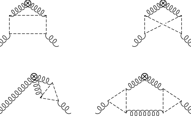
Figure 1: Graphs for $\omega_{1}$.

In [9], however, the structure of the QED $\beta$-function at $O(1/N_{\!f})$ was determined by explicitly carrying out the leading order bubble sum and using $\overline{\mbox{MS}}$ renormalization. This was later extended to the critical formalism in [10], which corresponds to the calculation of the first two graphs of figure 1. Therefore for the non-abelian extension one need only compute the remaining two graphs which involve the colour group factor $C_{2}(G)$. Although the critical exponent associated with the $\beta$-function is independent of the gauge parameter, to avoid mixing with the operator $(\partial^{\mu}A^{a}_{\mu})^{2}$, [11], we compute $\omega$ in the Landau gauge. With $b$ $=$ $0$ we find, [8],

$$\omega_{1}~{}=~{}-~{}\frac{C_{2}(G)\eta^{\mbox{o}}_{1}}{T(R)}\left[(2\mu-3)(\mu-3)\frac{C_{2}(R)}{C_{2}(G)}~{}-~{}\frac{(4\mu^{4}-18\mu^{3}+44\mu^{2}-45\mu+14)}{4(2\mu-1)(\mu-1)}\right]$$ (9)

where $\omega_{0}$ $=$ $(\mu-2)$. The $\epsilon$-expansion of (9) correctly reproduces the $3$-loop (gauge independent) result of [1-3] and allows us to deduce new coefficients at higher orders. In the notation of (1),

$$a_{4} = -~{}[154C_{2}(R)~{}+~{}53C_{2}(G)]/3888$$ (10)

$$a_{5} = C_{2}(R)(144\zeta(3)~{}+~{}107)/15552{}~{}+~{}C_{2}(G)(480\zeta(3)~{}-~{}229)/31104$$ (11)

where $\zeta(n)$ is the Riemann $\zeta$-function.

We close this section by noting some technical points in the determination of $\chi_{G}$ and anomalous dimensions of other operators. The contribution from each graph is found from the residue of the simple pole in the regulator of the critical theory, [12]. This (analytic) regularization is introduced by shifting the dimension of the gluon field by an infinitesimal amount, $\Delta$. In other words we calculate the graphs using (5) but with the replacement $\beta$ $\rightarrow$ $\beta$ $-$ $\Delta$. It is important to appreciate that the dimension of space-time is fixed in these exponent calculations, unlike in explicit perturbative computations using dimensional regularization.

4 POLARIZED OPERATORS

We have extended this analysis to other operators whose renormalization is necessary for the operator product expansion used in deep inelastic scattering. For instance, one can study the twist-$2$ flavour singlet polarized operators, [13],

$${\cal O}_{G} = \frac{i^{n}}{2}{\cal S}\epsilon^{\mu_{1}\alpha\beta\gamma}\mbox{tr}G_{\beta\gamma}D^{\mu_{2}}\ldots D^{\mu_{n-1}}G^{\mu_{n}}_{~{}~{}\,\alpha}$$

$${\cal O}_{F} = i^{n}{\cal S}\bar{\psi}\gamma^{5}\gamma^{\mu_{1}}D^{\mu_{2}}\ldots D^{\mu_{n}}\psi$$ (12)

where ${\cal S}$ denotes symmetrization in the Lorentz indices and subtraction of all combinations of traces and $n$ is the moment of the operator. The treatment of unpolarized flavour non-singlet and singlet operators at $O(1/N_{\!f})$ was given in [14]. We recall that the gauge independent anomalous dimension of these physical operators is responsible for the way in which the associated Wilson coefficients vary with energy. It is important to have large $N_{\!f}$ information available on the renormalization of (12) as the matrix of anomalous dimensions, $\gamma_{ij}(g)$, has recently been evaluated at second order, [15, 16]. A matrix of renormalization constants arises in perturbation theory due to the mixing under renormalization of both operators as they have the same quantum numbers and canonical dimensions, [14].

The computation of the corresponding exponent matrix, $\gamma_{ij}(g_{c})$, is by the technique outlined in the previous section. We substitute the operators in Green’s functions and determine the scaling behaviour. In the large $N_{\!f}$ approach there is a simplification. At criticality, due to the field content, the operators have different canonical dimensions and therefore do not mix. Alternatively this can be seen by calculating $\gamma_{ij}(g_{c})$ directly and observing that it is triangular at $O(1/N_{\!f})$, [14].

In order to relate exponent results to perturbation theory one observes that the exponent derived from the insertion of ${\cal O}_{F}$ actually corresponds to the eigenoperator of the perturbative mixing matrix which is predominantly fermionic in its content. In other words working at $g_{c}$ one circumvents the need to construct operators which diagonalize the RGE governing the evolution of the fermionic and gluonic singlet Wilson coefficients. The result of our calculation is, for even $n$,

$$\eta^{(n)}_{{\mbox{\footnotesize{F}}},1} = \frac{2C_{2}(R)\eta^{\mbox{o}}_{1}}{(2\mu-1)(\mu-2)T(R)}\left[\frac{}{}(\mu-1)^{2}{}~{}-~{}\frac{\mu(\mu-1)^{3}}{(\mu+n-1)(\mu+n-2)}\right.$$ (13)

$$\left.+~{}2\mu(\mu-1)[\psi(\mu-1+n)-\psi(\mu)]{}~{}-~{}\frac{\mu(2\mu+n-5)(n+2)S(n)}{2(\mu+n-1)(\mu+n-2)}\right]$$

where $S(n)$ $=$ $\Gamma(n)\Gamma(2\mu)/\Gamma(2\mu+n-2)$ and $\psi(x)$ is the logarithmic derivative of the $\Gamma$-function. It agrees with the two loop results of [15, 16] when $\gamma_{ij}(g)$ is diagonalized. The leading order $1/N_{\!f}$ value of the dimension of ${\cal O}_{G}$ is equivalent to the one loop value, which follows from the $N_{\!f}$ structure of the entries in $\gamma_{ij}(g)$. For the sake of comparison we note the exponent for the corresponding unpolarized operator ${\cal O}_{f}$ $=$ $i^{n}{\cal S}\bar{\psi}\gamma^{\mu_{1}}D^{\mu_{2}}$ $\ldots$ $D^{\mu_{n}}\psi$ is, [14],

$$\eta^{(n)}_{{\mbox{\footnotesize{f}}},1} = \frac{(\mu-1)C_{2}(R)\eta^{\mbox{o}}_{1}}{(2\mu-1)(\mu-2)T(R)N_{\!f}}\left[\frac{}{}2(\mu-1){}~{}-~{}\frac{2\mu(\mu-1)^{2}}{(\mu+n-1)(\mu+n-2)}\right.$$ (14)

$$+~{}\left.4\mu[\psi(\mu-1+n)-\psi(\mu)]\right.$$

$$-~{}\left.\frac{\mu(2\mu-1+n)\Gamma(n-1)\Gamma(2\mu)}{(\mu+n-1)(\mu+n-2)\Gamma(2\mu+n)}\right.$$

$$~{}~{}~{}~{}\times\left.[(n(n-1)+2(\mu-1+n))^{2}+2n(n-1)(\mu-2)(2\mu-3+2n)\right.$$

$$~{}~{}~{}~{}~{}~{}\left.+~{}4(\mu-2)(\mu-1+n)]\frac{}{}\right]$$

The purely four dimensional object $\gamma^{5}$ needs to be carefully treated in the large $N_{\!f}$ method, [17]. Unlike in some approaches in dimensional regularization we can use a fully anticommuting $\gamma^{5}$ in $d$-dimensions since our regularization is achieved by a shift in the gluon dimension, [18]. For closed fermion loops one performs the integral in $d$-dimensions before projecting with, for example, [17],

$$\mbox{tr}(\gamma^{5}\gamma^{\mu}\gamma^{\nu}\gamma^{\sigma}\gamma^{\rho})~{}=~{}4\epsilon_{\mu\nu\sigma\rho}$$ (15)

As a final application we have also computed the anomalous dimension of the singlet axial current, ${\cal O}_{5}$ $=$ $\bar{\psi}\gamma^{\mu}\gamma^{5}\psi$. The renormalization of this operator is more involved as it is not conserved in the quantum theory due to the chiral anomaly, [19]. However, in perturbation theory methods have been developed to obtain the three loop anomalous dimension in the $\overline{\mbox{MS}}$ scheme. (See, for example, [20].) Briefly this is a two part exercise. One part involves carrying out a standard $d$-dimensional renormalization using dimensional regularization. A finite renormalization is also required. This is determined by ensuring the one loop character of the operator form of the anomaly is preserved, [20]. A similar two part approach in $1/N_{\!f}$, using the above rules for graphs involving $\gamma^{5}$, yields the critical dimension of ${\cal O}_{5}$ as, [18],

$$\eta_{5,1}~{}=~{}-~{}\frac{3\mu C_{2}(R)\eta^{\mbox{o}}_{1}}{(\mu-1)T(R)}$$ (16)

The $\epsilon$-expansion of (16) agrees with the three loop result of [21, 20].

5 STRUCTURE FUNCTIONS

A second area of application of $1/N_{\!f}$ methods is in the determination of the higher order structure of the finite parts of Green’s functions or amplitudes. Not only are such calculations important in obtaining new coefficients of a series, they can also be used to study summability problems. As the $1/N_{\!f}$ approach is a reordering of perturbation theory in which graphs with infinite chains of quark loops are treated first, one could substitute such chains into the appropriate amplitude and carry out the renormalization to leave a finite result. In practice this will be tedious and inefficient. For a better approach we recall a feature of perturbative calculations. In dimensionally regularized calculations with massless fields, the effect of performing a quark loop integral is to obtain a $d$-dependent result with a factor which involves the momentum raised to a $d$-dependent power. In the renormalization process this latter part is important in obtaining the finite piece. Motivated by this and the simple structure of the fixed point propagators, we can obtain $O(1/N_{\!f})$ information on the finite part efficiently by using the propagators, [14],

$$\psi(k) = \frac{k\!\!\!/}{k^{2}}$$

$$A_{\mu\nu}(k) = \frac{1}{(k^{2})^{1+\delta}}\left[\eta_{\mu\nu}{}~{}-~{}\frac{k_{\mu}k_{\nu}}{k^{2}}\right]$$ (17)

We stress that this approach is not at a fixed point and is closer in spirit to perturbative calculations. The gluon propagator has an adjusted power, $\delta$, where $\delta$ $=$ $4N_{\!f}T(R)g/3$. Calculations are performed by substituting (13) into Green’s functions with undressed gluon lines with the integration restricted to four dimensions. The resulting $\delta$-dependent function can be expanded in powers of $\delta$ and it transpires that the coefficients are in direct correspondence with those obtained in perturbation theory.

Several applications are available. For instance, the finite part of the photon propagator has been determined in QED, [22]. In deep inelastic scattering the $O(1/N_{\!f})$ part of the longitudinal non-singlet structure function has been studied. The Wilson coefficients at the $L$th loop is, [14],

$$C^{\mbox{\footnotesize{NS}}}_{\mbox{\footnotesize{long}}}(1,g,L)~{}=~{}\frac{d^{L}~{}}{d\delta^{L}}\!\left[\frac{8C_{2}(R)e^{5\delta/3}\bar{S}(n,\delta)g}{(2-\delta)(1-\delta)x^{n}}\right]$$ (18)

where $\bar{S}(n,\delta)$ $=$ $\Gamma(n+\delta)/[\Gamma(n)\Gamma(1+\delta)/(n+1+\delta)]$, and $x$ is the Bjorken scaling variable. It agrees with the three loop results of [23].

The poles in $\delta$ at $\delta$ $=$ $1$ and $2$ correspond to renormalons in the series. Recently, these have been used with the naive non-abelianization procedure, [24], to estimate the effect of higher twist contributions to the full structure function, [25]

6 CONCLUSIONS

We have focussed primarily on the $O(1/N_{\!f})$ corrections to the RGE functions. One important feature of the fixed point approach, however, is that $O(1/N_{\!f}^{2})$ calculations are also possible in $d$-dimensions. For example, the anomalous dimension of the electron mass in QED has been determined at this order, [26]. With the simplification that occurs from the equivalence of QCD and NATM the extension of this and other results will be possible for the non-abelian case.

References

- [1] D.J. Gross and F.J. Wilczek, Phys. Rev. Lett. 30 (1973) 1343; H.D. Politzer, Phys. Rev. Lett. 30 (1973) 1346.
- [2] W.E. Caswell, Phys. Rev. Lett. 33 (1974) 244; D.R.T. Jones, Nucl. Phys. B75 (1974) 531.
- [3] O.V. Tarasov, A.A. Vladimirov and A.Yu. Zharkov, Phys. Lett. 93B (1980) 429; S.A. Larin and J.A.M. Vermaseren, Phys. Lett. B303 (1993) 334.
- [4] A.N. Vasil’ev, Yu.M. Pis’mak and J.R. Honkonen, Theor. Math. Phys. 46 (1981) 157; Theor. Math. Phys. 47 (1981) 291.
- [5] J. Zinn-Justin, Quantum Field Theory and Critical Phenomena, Clarendon Press, Oxford, 1989.
- [6] J.A. Gracey, Phys. Lett. B318 (1993) 177.
- [7] A. Hasenfratz and P. Hasenfratz, Phys. Lett. B297 (1992) 166.
- [8] J.A. Gracey, hep-ph/9602214.
- [9] A. Palanques-Mestre and P. Pascual, Commun. Math. Phys. 95 (1984) 277.
- [10] J.A. Gracey, Int. J. Mod. Phys. A8 (1993) 2465.
- [11] A.N. Vasil’ev, M.Yu. Nalimov and J.R. Honkonen, Theor. Math. Phys. 58 (1984), 111.
- [12] A.N. Vasil’ev and M.Yu. Nalimov, Theor. Math. Phys. 55 (1982) 423; Theor. Math. Phys. 56 (1982) 643.
- [13] M.A. Ahmed and G.G. Ross, Nucl. Phys. B111 (1976), 441.
- [14] J.A. Gracey, Phys. Lett. B322 (1994) 141; hep-ph/9609276.
- [15] R. Mertig and W.L. van Neerven, hep-ph/9506451.
- [16] W. Vogelsang, hep-ph/9603366.
- [17] G. ’t Hooft and M. Veltman, Nucl. Phys. B44 (1972) 189.
- [18] J.A. Gracey, paper in preparation.
- [19] S.L. Adler, Phys. Rev. 177 (1969) 2426; J.S. Bell and R. Jackiw, Nuovo Cim. 60A (1969) 47; S.L. Adler and W. Bardeen, Phys. Rev. 182 (1969) 1517.
- [20] S.A. Larin, Phys. Lett. B303 (1993) 113.
- [21] J. Kodaira, Nucl. Phys. B165 (1980) 129.
- [22] D.J. Broadhurst, Z. Phys. C58 (1993) 339; M. Beneke, Nucl. Phys. B405 (1993), 424.
- [23] S.A. Larin, T. van Ritbergen and J.A.M. Vermaseren, Nucl. Phys. B427 (1994) 41.
- [24] M. Beneke and V.M. Braun, Phys. Lett. B348 (1995) 513; D.J. Broadhurst and A.G. Grozin, Phys. Rev. D52 (1995) 4082.
- [25] E. Stein, M. Meyer-Hermann, L. Mankiewicz and A. Schäfer, hep-ph/9601356.
- [26] J.A. Gracey, Phys. Lett. B317 (1993) 415.