Renormalization and Chiral Symmetry Breaking in Quenched QED in Arbitrary Covariant Gauge

Abstract

We extend a previous Landau-gauge study of subtractive renormalization of the fermion propagator Dyson-Schwinger equation (DSE) in strong-coupling, quenched QED₄ to arbitrary covariant gauges. We use the fermion-photon proper vertex proposed by Curtis and Pennington with an additional correction term included to compensate for the small gauge-dependence induced by the ultraviolet regulator. We discuss the chiral limit and the onset of dynamical chiral symmetry breaking in the presence of nonperturbative renormalization. We extract the critical coupling in several different gauges and find evidence of a small residual gauge-dependence in this quantity.

I Introduction

Strong coupling QED₄ has been studied for some time within the Dyson-Schwinger equation (DSE) formalism both for its intrinsic interest and also as the basis for abelianized models of nonperturbative phenomena in technicolor theories and QCD. For recent reviews of Dyson-Schwinger equations and their application and numerous references see for example Refs. [1, 2, 3]. The usual approach is to write the DSE for the fermion propagator or self-energy, possibly including equations for the photon vacuum polarization or the fermion-photon proper vertex. In a recent study [4] it was shown for the first time how to implement nonperturbative renormalization in a numerical way within the DSE formalism. In that work the calculations were carried out in quenched approximation in Landau gauge. Here we will extend these studies to arbitrary covariant gauges and will also discuss the chiral limit.

The DSE’s are an infinite tower of coupled integral equations and so it is always necessary to truncate this tower at some point and introduce an Ansatz for any necessary undefined Green’s functions. It is of course important to ensure that this Ansatz be consistent with all appropriate symmetries of the theory and that it have the correct perturbative limit. The resulting nonlinear integral equations are solved numerically in Euclidean space by iteration. Dynamical (or spontaneous) chiral symmetry breaking (DCSB) occurs when the fermion propagator develops a nonzero scalar self-energy in the absence of an explicit chiral symmetry breaking (ECSB) fermion mass. We will refer to coupling constants strong enough to induce DCSB as supercritical and those weaker are called subcritical. We write the fermion propagator as

$$S(p)=\frac{Z(p^{2})}{\not\!p-M(p^{2})}=\frac{1}{A(p^{2})\not\!p-B(p^{2})}$$ (1)

where we refer to $A(p^{2})\equiv 1/Z(p^{2})$ as the finite momentum-dependent fermion renormalization and where $M(p^{2})\equiv B(p^{2})/A(p^{2})$ is the fermion mass function. In the massless theory (i.e., in the absence of an ECSB bare fermion mass) by definition DCSB occurs when $M(p^{2})\neq 0$.

Until relatively recently, most studies have used the bare vertex as an Ansatz for the one-particle irreducible (1-PI) vertex $\Gamma^{\nu}(k,p)$, [5, 6, 7, 8, 9] despite the fact that this violates the Ward-Takahashi Identity (WTI) [10]. The resulting fermion propagator is not gauge-covariant, i.e., physical quantities such as the critical coupling for dynamical symmetry breaking and the fermion mass pole are gauge-dependent [11, 12, 13]. There have been several studies which attempted to make the fermion DSE gauge-covariant by using improved vertex forms which satisfy the WTI but which possess kinematic singularities in the limit of zero photon momentum [13, 14]. A general form for $\Gamma^{\nu}(k,p)$ which does satisfy the Ward Identity and which has no unphysical kinematic singularities was given by Ball and Chiu in 1980 [15]; it consists of a minimal longitudinally constrained term which satisfies the WTI, and a set of tensors spanning the subspace transverse to the photon momentum $q$.

While the WTI is necessary for gauge-invariance, it is not a sufficient condition and in itself does not ensure gauge covariance of the fermion propagator. Furthermore, with many vertex Ansätze the fermion propagator DSE is not multiplicatively renormalizable, which is equivalent to saying that overlapping logarithms are present. There has been much recent research on the use of the transverse parts of the vertex to ensure both gauge-covariant and multiplicatively renormalizable solutions [12, 16, 17, 18, 19, 20, 21, 22, 23, 24], some of which will be discussed below.

With the exception of Ref. [4], studies have mostly neglected the issue of the subtractive renormalization of the DSE for the fermion propagator. Typically these studies have assumed an initially massless theory and have renormalized at the ultraviolet cutoff of the loop integration, taking $Z_{1}=Z_{2}=1$. Where a nonzero bare mass has been used, it has simply been added to the scalar term in the propagator. While in some circumstances for the special case of Landau gauge this can be a reasonable approximation, it is in general incorrect. Although there have been earlier formal discussions of renormalization [2, 12, 19], the important step of subtractive renormalization had not been performed prior to the recent study in Landau gauge [4].

Here we present the results of a study of subtractive renormalization in the fermion DSE in arbitrary covariant gauge for quenched strong-coupling QED₄. Note that here the term “quenched” means that the bare photon propagator is used in the fermion self-energy DSE, so that $Z_{3}=1$ and there is no renormalization of the electron charge. This is a somewhat different usage to that found in lattice gauge theory studies, since in our study virtual fermion loops may still be present in the proper fermion-photon vertex.

The organization of the paper is as follows: The formalism is discussed in Sec. II. This section contains discussions of the DSE for the renormalized fermion propagator, the Ansätze for the proper vertex, the subtractive renormalization procedure, the chiral limit, and renormalization point transformations. Our detailed numerical results are presented in Sec. III and we present our summary and conclusions in Sec. IV.

II Formalism

A Renormalized DSE

The DSE for the renormalized fermion propagator, in an arbitrary covariant gauge, is

$$S^{-1}(p)=Z_{2}(\mu,\Lambda)[\not\!p-m_{0}(\Lambda)]-iZ_{1}(\mu,\Lambda)e^{2}\int^{\Lambda}\frac{d^{4}k}{(2\pi)^{4}}\gamma^{\mu}S(k)\Gamma^{\nu}(k,p)D_{\mu\nu}(q)\>;$$ (2)

here $q=k-p$ is the photon momentum, $\mu$ is the renormalization point, and $\Lambda$ is a regularizing parameter (taken here to be an ultraviolet momentum cutoff). We write $m_{0}(\Lambda)$ for the regularization-parameter dependent bare mass. The renormalized charge is $e$ (as opposed to the bare charge $e_{0}$), and the general form for the renormalized photon propagator is

$$D^{\mu\nu}(q)=\left\{\left(-g^{\mu\nu}+\frac{q^{\mu}q^{\nu}}{q^{2}}\right)\frac{1}{1+\Pi(q^{2})}-\xi\frac{q^{\mu}q^{\nu}}{q^{2}}\right\}\frac{1}{q^{2}}\>,$$ (3)

with $\xi$ the renormalized covariant gauge parameter and $\xi_{0}\equiv Z_{3}(\mu,\Lambda)\xi$ the corresponding bare one. Since we work in the quenched approximation, we have for the coupling strength and gauge parameter respectively $\alpha\equiv e^{2}/4\pi=\alpha_{0}\equiv e_{0}^{2}/4\pi$ and $\xi=\xi_{0}$, and for the photon propagator we have

$$D^{\mu\nu}(q)\to D_{0}^{\mu\nu}(q)=\left\{\left(-g^{\mu\nu}+\frac{q^{\mu}q^{\nu}}{q^{2}}\right)-\xi\frac{q^{\mu}q^{\nu}}{q^{2}}\right\}\frac{1}{q^{2}}\>.$$ (4)

B Vertex Ansatz

The requirement of gauge invariance in QED leads to a set of identities referred to as the Ward-Takahashi Identities (WTI). The WTI for the fermion-photon vertex is

$$q_{\mu}\Gamma^{\mu}(k,p)=S^{-1}(k)-S^{-1}(p)\;,$$ (5)

where $q=k-p$ . This is a generalization of the original differential Ward identity, which expresses the effect of inserting a zero-momentum photon vertex into the fermion propagator,

$$\frac{\partial S^{-1}(p)}{\partial p_{\nu}}=\Gamma^{\nu}(p,p)\>.$$ (6)

The Ward identity Eq. (6) follows immediately from the WTI of Eq. (5) after setting to zero all but the $\nu$ component of $q$, dividing both sides of the WTI by $q_{\nu}$ and then taking $q_{\nu}\to 0$. In general, for nonvanishing photon momentum $q$, only the longitudinal component of the proper vertex is constrained, i.e., the WTI provides no information on $\Gamma^{\nu}_{\rm T}(k,p)\equiv{\cal T}^{\mu\nu}\Gamma_{\nu}(p,k)$ for $q\neq 0$. [We use the notation ${\cal T}^{\mu\nu}\equiv g^{\mu\nu}-(q^{\mu}q^{\nu}/q^{2})$ and ${\cal L}^{\mu\nu}\equiv(q^{\mu}q^{\nu}/q^{2})$ for the transverse and longitudinal projectors respectively.] In particular, the WTI guarantees the equality of the propagator and vertex renormalization constants, $Z_{2}\equiv Z_{1}$ (at least in any reasonable subtraction scheme [1].) The WTI can be shown to be satisfied order-by-order in perturbation theory and can also be derived nonperturbatively.

As discussed in [1, 25], this can be thought of as just one of a set of six general requirements on the vertex: (i) the vertex must satisfy the WTI; (ii) it should contain no kinematic singularities; (iii) it should transform under charge conjugation ($C$), parity inversion ($P$), and time reversal ($T$) in the same way as the bare vertex, e.g.,

$$C^{-1}\Gamma_{\mu}(k,p)C=-\Gamma_{\mu}^{\rm T}(-p,-k)$$ (7)

(where the superscript T indicates the transpose); (iv) it should reduce to the bare vertex in the weak-coupling limit; (v) it should ensure multiplicative renormalizability of the DSE in Eq. (2); (vi) the transverse part of the vertex should be specified to ensure gauge-covariance of the DSE.

Ball and Chiu [15] have given a description of the most general fermion-photon vertex that satisfies the WTI; it consists of a longitudinally-constrained (i.e., “Ball-Chiu”) part $\Gamma^{\mu}_{\rm BC}$, which is a minimal solution of the WTI, and a basis set of eight transverse vectors $T_{i}^{\mu}(k,p)$, which span the hyperplane specified by ${\cal L}_{\mu\nu}T_{i}^{\nu}(k,p)=0$ (i.e., $q_{\nu}T_{i}^{\nu}(k,p)=0$), where $q\equiv k-p$. The minimal longitudinally constrained part of the vertex will be referred to as the Ball-Chiu vertex and is given by

$$\Gamma^{\mu}_{\rm BC}(k,p)=\frac{1}{2}[A(k^{2})+A(p^{2})]\gamma^{\mu}+\frac{(k+p)^{\mu}}{k^{2}-p^{2}}\left\{[A(k^{2})-A(p^{2})]\frac{{\not\!k}+{\not\!p}}{2}-[B(k^{2})-B(p^{2})]\right\}\>.$$ (8)

Note that since neither ${\cal L}_{\mu\nu}\Gamma^{\nu}_{\rm BC}(k,p)$ nor ${\cal T}_{\mu\nu}\Gamma^{\nu}_{\rm BC}(k,p)$ vanish identically, the Ball-Chiu vertex has both longitudinal and transverse components. The transverse tensors can be conveniently written as [26]

$$T_{1}^{\mu}(k,p) = p^{\mu}(k\cdot q)-k^{\mu}(p\cdot q)\>,$$ (9)

$$T_{2}^{\mu}(k,p) = \left[p^{\mu}(k\cdot q)-k^{\mu}(p\cdot q)\right]({\not\!k}+{\not\!p})\>,$$ (10)

$$T_{3}^{\mu}(k,p) = q^{2}\gamma^{\mu}-q^{\mu}{\not\!q}\>,$$ (11)

$$T_{4}^{\mu}(k,p) = q^{2}\left[\gamma^{\mu}(\not\!p+\not\!k)-p^{\mu}-k^{\mu}\right]-2i(p-k)^{\mu}k^{\lambda}p^{\nu}\sigma_{\lambda\nu}\>,$$ (12)

$$T_{5}^{\mu}(k,p) = -iq_{\nu}{\sigma^{\nu\mu}}\>,$$ (13)

$$T_{6}^{\mu}(k,p) = \gamma^{\mu}(p^{2}-k^{2})+(p+k)^{\mu}{\not\!q}\>,$$ (14)

$$T_{7}^{\mu}(k,p) = \frac{1}{2}(p^{2}-k^{2})\left[\gamma^{\mu}({\not\!p}+{\not\!k})-p^{\mu}-k^{\mu}\right]-i\left(k+p\right)^{\mu}k^{\lambda}p^{\nu}\sigma_{\lambda\nu}\>,$$ (15)

$$T_{8}^{\mu}(k,p) = i\gamma^{\mu}k^{\nu}p^{\lambda}{\sigma_{\nu\lambda}}+k^{\mu}{\not\!p}-p^{\mu}{\not\!k}\>,$$ (16)

where we use the conventions $g^{\mu\nu}={\rm diag}(1,-1,-1,-1)$, $\{\gamma^{\mu},\gamma^{\nu}\}=2g^{\mu\nu}$, and $\sigma^{\mu\nu}\equiv(i/2)[\gamma^{\mu},\gamma^{\nu}]$. Note that these tensors have been written in a different linear combination to the ones presented in Ref. [4]. A general vertex is then written as

$$\Gamma^{\mu}(k,p)=\Gamma_{BC}^{\mu}(k,p)+\sum_{i=1}^{8}\tau_{i}(k^{2},p^{2},q^{2})T_{i}^{\mu}(k,p)\>,$$ (17)

where the $\tau_{i}$ are functions that must be chosen to give the correct $C$, $P$, and $T$ invariance properties.

Curtis and Pennington published a series of articles [12, 19, 20, 21] describing their specification of a particular transverse vertex term, in an attempt to produce gauge-covariant and multiplicatively renormalizable solutions to the DSE. In the framework of massless QED₄, they eliminated the four transverse vectors which are Dirac-even and must generate a scalar term. By requiring that the vertex $\Gamma^{\mu}(k,p)$ reduce to the leading log result for $k\gg p$ they were led to eliminate all the transverse basis vectors except $T_{6}^{\mu}$, with a dynamic coefficient chosen to make the DSE multiplicatively renormalizable. This coefficient had the form

$$\tau_{6}(k^{2},p^{2},q^{2})=-\frac{1}{2}[A(k^{2})-A(p^{2})]/d(k,p)\>,$$ (18)

where $d(k,p)$ is a symmetric, singularity-free function of $k$ and $p$, with the limiting behavior $\lim_{k^{2}\gg p^{2}}d(k,p)=k^{2}$. [Here, $A(p^{2})\equiv 1/Z(p^{2})$ is their $1/{\cal F}(p^{2})$.] For purely massless QED, they found a suitable form, $d(k,p)=(k^{2}-p^{2})^{2}/(k^{2}+p^{2})$. This was generalized to the case with a dynamical mass $M(p^{2})$, to give

$$d(k,p)=\frac{(k^{2}-p^{2})^{2}+[M^{2}(k^{2})+M^{2}(p^{2})]^{2}}{k^{2}+p^{2}}\>.$$ (19)

They then showed that multiplicative renormalizability is retained up to next-to-leading-log order in the DCSB case. Subsequent papers established the form of the solutions for the renormalization and the mass [21] and studied the gauge-dependence of the solutions [12]. Dong, Munczek and Roberts [22] subsequently showed that the lack of exact gauge-covariance of the solutions was due to the use of a momentum cutoff in the integral equations, since this type of regularization is not Poincaré invariant. The fact that there is still some residual gauge-dependence in the physical observables such as the chiral critical point shows that with a momentum cutoff the C-P vertex Ansatz is not yet the ideal choice. Dong, Munczek and Roberts [22] derived an Ansatz for the transverse vertex terms which satisfies the WTI and makes the fermion propagator gauge-covariant under hard momentum-cutoff regularization.

Bashir and Pennington [23, 24] subsequently described two different vertex Ansätze which make the fermion self-energy exactly gauge-covariant, in the sense that the critical point for the chiral phase transition is independent of gauge. Specific constraints they have assumed for the vertex are, in [23] that the transverse vertex parts vanish in the Landau gauge, and in [24] that the anomalous dimension of the fermion mass function $\gamma_{m}$ is exactly 1 at the critical coupling. Their work is a continuation of that of Dong, Munczek and Roberts, and indeed their vertex Ansatz corresponds to the general form suggested in [22].

However, the kinematic factors $\tau_{2,3,6,8}$ in both vertex forms are rather complicated and depend upon a pair of as yet undetermined functions $W_{1,2}(k^{2},p^{2})$ which must be chosen to guarantee that the weak-coupling limit of $\Gamma^{\mu}$ matches the perturbative result. Renormalization studies of the DSE using these new vertex Ansätze should be interesting and represent a direction for further research.

For the solutions to the fermion DSE using the C-P vertex, the critical point for the chiral phase transition has been shown to have a much weaker gauge-dependence than that for the DSE with the bare or minimal Ball-Chiu vertices [27]. In this work we will use the Curtis-Pennington Ansatz as the basis for our calculations.

The equations are separated into a Dirac-odd part describing the finite propagator renormalization $A(p^{2})$, and a Dirac-even part for the scalar self-energy, by taking $\frac{1}{4}{\rm Tr}$ of the DSE multiplied by $\not\!p/p^{2}$ and 1, respectively. The equations are solved in Euclidean space and so the volume integrals $\int d^{4}k$ can be separated into angle integrals and an integral $\int dk^{2}$; the angle integrals are easy to perform analytically, yielding the two equations which will be solved numerically.

One refinement of our treatment of the C-P vertex in the present work is associated with subtleties in the ultraviolet regularization scheme. Although there have been some exploratory studies of dimensional regularization for the DSE [28], this has not yet proven practical in nonperturbative field theory and momentum cutoffs for now remain the regularization scheme of choice in such studies. Naive imposition of a momentum cutoff destroys the gauge covariance of the DSE because the self-energy integral contains terms, related to the vertex WTI, which should vanish but which are nonzero when integrated under cutoff regularization [22, 23]. In Appendix A we derive an expression for one such undesirable term and show how it may subtracted in a simple way from the regularized self-energy. We have also calculated some DSE solutions with the usual uncorrected UV cut-off method for comparison purposes, but otherwise we use this “gauge-improved” regularization combined with the C-P vertex throughout this work. This will be commented on futher in the discussion of numerical results in Sec. III.

C Subtractive Renormalization

The subtractive renormalization of the fermion propagator DSE proceeds similarly to the one-loop renormalization of the propagator in QED. (This is discussed in [1] and in [29], p. 425ff.) One first determines a finite, regularized self-energy, which depends on both a regularization parameter and the renormalization point; then one performs a subtraction at the renormalization point, in order to define the renormalization parameters $Z_{1}$, $Z_{2}$, $Z_{3}$ which give the full (renormalized) theory in terms of the regularized calculation.

A review of the literature of DSEs in QED shows, however, that this step is never actually performed. Curtis and Pennington [12] for example, define their renormalization point at the UV cutoff.

Many studies take $Z_{1}=Z_{2}=1$ [12, 16, 18, 19, 20, 21]; this is a reasonable approximation in Landau gauge in cases where the coupling $\alpha$ is sufficiently small (i.e., $\alpha$ $\stackrel{{\scriptstyle<}}{{\sim}}$ 1), but if $\alpha$ is chosen large enough, the value of the dynamical mass at the renormalization point may be significantly large compared with its maximum in the infrared. For instance, in Ref. [12], figures for the fermion mass are given with $\alpha$ = 0.97, 1.00, 1.15 and 2.00 in various gauges. For $\alpha=2.00$, the fermion mass at the cutoff is down by only an order of magnitude from its limiting value in the infrared. In general for strong coupling and/or gauges other than Landau gauge this approximation is unreliable.

As shown in Ref. [4] subtractive renormalization can be properly implemented in numerical DSE studies without such approximations. We begin with a summary of the renormalization procedure [1, 4]. One defines a regularized self-energy $\Sigma^{\prime}(\mu,\Lambda;p)$, leading to the DSE for the renormalized fermion propagator,

$$\widetilde{S}^{-1}(p) = Z_{2}(\mu,\Lambda)[\not\!p-m_{0}(\Lambda)]-\Sigma^{\prime}(\mu,\Lambda;p)$$ (20)

$$= \not\!p-m(\mu)-\widetilde{\Sigma}(\mu;p)=A(p^{2})\not\!p-B(p^{2})\>,$$ (21)

where the (regularized) self-energy is

$$\Sigma^{\prime}(\mu,\Lambda;p)=iZ_{1}(\mu,\Lambda)e^{2}\int^{\Lambda}\frac{d^{4}k}{(2\pi)^{4}}\gamma^{\lambda}\widetilde{S}(\mu;k)\widetilde{\Gamma}^{\nu}(\mu;k,p)\widetilde{D}_{\lambda\nu}(\mu;(p-k))\>.$$ (22)

[To avoid confusion we will follow Ref. [1] and in this section only we will denote regularized quantities with a prime and renormalized ones with a tilde, e.g. $\Sigma^{\prime}(\mu,\Lambda;p)$ is the regularized self-energy depending on both the renormalization point $\mu$ and regularization parameter $\Lambda$ and $\widetilde{\Sigma}(\mu;p)$ is the renormalized self-energy.] As suggested by the notation (i.e., the omission of the $\Lambda$-dependence) renormalized quantities must become independent of the regularization-parameter as the regularization is removed (i.e., as $\Lambda\to\infty$). The self-energies are decomposed into Dirac and scalar parts,

$$\Sigma^{\prime}(\mu,\Lambda;p)=\Sigma^{\prime}_{d}(\mu,\Lambda;p^{2})\not\!p+\Sigma^{\prime}_{s}(\mu,\Lambda;p^{2})$$ (23)

(and similarly for the renormalized quantity, $\widetilde{\Sigma}(\mu,p)$). By imposing the renormalization boundary condition,

$$\left.\widetilde{S}^{-1}(p)\right|_{p^{2}=\mu^{2}}=\not\!p-m(\mu)\>,$$ (24)

one gets the relations

$$\widetilde{\Sigma}_{d,s}(\mu;p^{2})=\Sigma^{\prime}_{d,s}(\mu,\Lambda;p^{2})-\Sigma^{\prime}_{d,s}(\mu,\Lambda;\mu^{2})$$ (25)

for the self-energy,

$$Z_{2}(\mu,\Lambda)=1+\Sigma^{\prime}_{d}(\mu,\Lambda;\mu^{2})$$ (26)

for the renormalization constant, and

$$m_{0}(\Lambda)=\left[m(\mu)-\Sigma^{\prime}_{s}(\mu,\Lambda;\mu^{2})\right]/Z_{2}(\mu,\Lambda)$$ (27)

for the bare mass. The mass renormalization constant is then given by

$$Z_{m}(\mu,\Lambda)=m_{0}(\Lambda)/m(\mu)\>,$$ (28)

i.e., as the ratio of the bare to renormalized mass.

The vertex renormalization, $Z_{1}(\mu,\Lambda)$, is identical to $Z_{2}(\mu,\Lambda)$ as long as the vertex Ansatz satisfies the Ward Identity; this is how it is recovered for multiplication into $\Sigma^{\prime}(\mu,\Lambda;p)$ in Eq. (22).

In order to obtain numerical solutions, the final Minkowski-space integral equations are first rotated to Euclidean space. [Note that all equations in Secs. I and II are written in Minkowski space.] They are then solved by iteration on a logarithmic grid from an initial guess. The solutions are confirmed to be independent of the initial guess and are solved with a wide range of cutoffs ($\Lambda$), renormalization points ($\mu$), couplings ($\alpha$), covariant gauge choices ($\xi$), and renormalized masses ($m(\mu)$).

The chiral limit occurs by definition when the bare mass is taken to zero sufficiently rapidly as the regularization is removed. This is guaranteed, for example, by maintaining $m_{0}(\Lambda)=0$ as $\Lambda\to\infty$. Explicit chiral symmetry breaking (ECSB) occurs when the bare mass $m_{0}(\Lambda)$ is not zero, (or more precisely, whenever it is not taken to zero sufficiently rapidly as $\Lambda\to\infty$). Dynamical chiral symmetry breaking (DCSB) is said to have occured when $M(p^{2})\not=0$ in the absence of ECSB. As the coupling strength increases from zero, there is a transition to a DCSB phase at the critical coupling $\alpha_{c}$. Concisely, the absence of ECSB means that we can set $m_{0}(\Lambda)=0$, and the absence of both ECSB and DCSB (i.e., $\alpha<\alpha_{c}$) means that $M(p^{2})$, $m(\mu)$, and $m_{0}(\Lambda)$ simultaneously vanish. (Recall that in the notation that we use here, $M(p^{2})\equiv B(p^{2})/A(p^{2})$ and $m(\mu)\equiv M(\mu^{2})$.) This is the same definition of the chiral limit that is used in nonperturbative studies of QCD, see e.g. Refs. [1, 2, 3, 30] and references therein. Obviously, any limiting procedure where we take $m_{0}(\Lambda)\to 0$ sufficiently rapidly as $\Lambda\to\infty$ will also lead to the chiral limit [2].

D Renormalization Point Transformations

A renormalization point transformation is a change of renormalization scale [i.e., ${\cal R}(\mu,\mu^{\prime})$ for $\mu\to\mu^{\prime}$] such that the bare mass(es) and coupling(s) remain fixed for fixed regularization parameter ($\Lambda$) and fixed renormalization scheme. This ensures that the physical observables of the theory are invariant under such a transformation. This set of transformations is associative [${\cal R}(\mu,\mu^{\prime}){\cal R}(\mu^{\prime},\mu^{\prime\prime})={\cal R}(\mu,\mu^{\prime\prime})$], contains the identity [${\cal R}(\mu,\mu)={\cal I}$], and contains all inverses [${\cal R}(\mu,\mu^{\prime})^{-1}={\cal R}(\mu^{\prime},\mu)$] and hence is called the renormalization group.

For the purposes of the discussion here we will now explicitly indicate the choice of renormalization point by a $\mu$-dependence of the renormalized quantities, i.e., $A(\mu;p^{2})\equiv 1/Z(\mu;p^{2})$, $M(\mu;p^{2})\equiv B(\mu;p^{2})/A(\mu;p^{2})$, etc. Note that Eq. (20) implies that

$$A(\mu;p^{2}) = Z_{2}(\mu,\Lambda)-\Sigma^{\prime}_{d}(\mu,\Lambda;p^{2})=1-\widetilde{\Sigma}_{d}(\mu,\Lambda;p^{2})\;,$$ (29)

$$B(\mu;p^{2}) = Z_{2}(\mu,\Lambda)m_{0}(\Lambda)+\Sigma^{\prime}_{s}(\mu,\Lambda;p^{2})=m(\mu)+\widetilde{\Sigma}_{s}(\mu,\Lambda;p^{2})\;.$$ (30)

The renormalization point boundary condition in Eq. (24) then leads to $\widetilde{\Sigma}(\mu,\Lambda;\mu^{2})=0$, or equivalently, to the two boundary conditions $A(\mu;\mu^{2})=1$ and $M(\mu;\mu^{2})=B(\mu;\mu^{2})=m(\mu)$. From Eq. (30) and the fact that $Z_{1}(\mu,\Lambda)=Z_{2}(\mu,\Lambda)$ we have

$$\left[A(\mu;p^{2})/Z_{2}(\mu,\Lambda)\right] = 1-\left[\Sigma^{\prime}_{d}(\mu,\Lambda;p^{2})/Z_{1}(\mu,\Lambda)\right]\;,$$ (31)

$$\left[B(\mu;p^{2})/Z_{2}(\mu,\Lambda)\right] = m_{0}(\Lambda)+\left[\Sigma^{\prime}_{s}(\mu,\Lambda;p^{2})/Z_{1}(\mu,\Lambda)\right]\;.$$ (32)

Consider the effects of an an arbitrary rescaling $A(p^{2})\to cA(p^{2})$ and $B(p^{2})\to cB(p^{2})$, [i.e., $M(p^{2})$ fixed], for some real constant $c$. It is straightforward to see that under such a rescaling we have $S(p)\to(1/c)S(p)$ and $\Gamma^{\nu}(p^{\prime},p)\to c\Gamma^{\nu}(p^{\prime},p)$. It follows that the RH sides of Eqs. (32) are unaffected by such an arbitrary rescaling. Hence, it follows that the choice of renormalization point boundary conditions is equivalent to the choice of scale for the functions $A$ and $B$.

Let us consider this observation in more detail. Since we are working in the quenched approximation, where $e^{2}$ and $\widetilde{D}$ are unaffected by a change of renormalization point, it follows from Eq. (22) that $\Sigma^{\prime}(\mu,\Lambda;p^{2})/Z_{1}(\mu,\Lambda)$ is renormalization point independent since a change of renormalization point is a rescaling of $A$ and $B$. Then since $m_{0}(\Lambda)$ is renormalization point independent by definition, the entire RHS of Eqs. (32) must be independent of the choice of renormalization point. Thus, under a renormalization point transformation we must have for all $p^{2}$

$$M(\mu^{\prime};p^{2}) = M(\mu;p^{2})\equiv M(p^{2})\;,$$ (33)

$$\frac{A(\mu^{\prime};p^{2})}{A(\mu;p^{2})} = \frac{Z_{2}(\mu^{\prime},\Lambda)}{Z_{2}(\mu,\Lambda)}=A(\mu^{\prime};\mu^{2})=\frac{1}{A(\mu;\mu^{\prime 2})}\;,$$ (34)

from which it follows for the fermion propagator that $\widetilde{S}(\mu^{\prime};p)/\tilde{S}(\mu;p)=Z_{2}(\mu,\Lambda)/Z_{2}(\mu^{\prime},\Lambda)$ in the usual way. The behavior in Eq. (34) is explicitly tested for our numerical solutions. It is clear from Eq. (34) that having a solution at one renormalization point ($\mu$) completely determines the solution at any other renormalization point ($\mu^{\prime}$) without the need for any further computation.

An alternative derivation of this result which starts from the renormalized action and which applies to the general unquenched case can be found for example in Sec. 2.1 of Ref. [1]. For brevity we can denote the above renormalization point dependence of the fermion propagator by $\widetilde{S}(\mu;p)\propto 1/Z_{2}(\mu,\Lambda)$. In the general unquenched case [29] we would have in addition $\widetilde{D}^{\sigma\nu}(\mu;q)\propto\xi(\mu)\propto 1/Z_{3}(\mu,\Lambda)$, $e(\mu)\propto Z_{2}(\mu,\Lambda)\sqrt{Z_{3}(\mu,\Lambda)}/Z_{1}(\mu,\Lambda)$, and $e(\mu)\widetilde{\Gamma}^{\nu}(\mu;q,p)\propto Z_{2}(\mu,\Lambda)\sqrt{Z_{3}(\mu,\Lambda)}$.

III Results

Solutions were obtained in Euclidean space for the DSE for couplings $\alpha$ from 0.1 to 1.30, in gauges with $\xi$ from -0.25 to 3, and with a variety of renormalization points and renormalized masses. All results in this section refer to Euclidean space quantities. In the graphs and tables that follow, there are no explicit mass units. Since the equations have no inherent mass-scale, the cutoff $\Lambda$, renormalization point $\mu$, $m(\mu)$, and units of $M(p^{2})$ or $B(p^{2})$ all scale multiplicatively, and the units are arbitrary. In four dimensions the coupling has no mass dimension, therefore it remains unchanged for all such choices of mass units.

Fig. 1 shows a family of solutions characterized by $\alpha=1.00$, $\mu^{2}=1\times 10^{8}$, $m(\mu)=400$, and gauge parameters from -0.25 to 1.25. We see that while $A$ and $B$ are strongly gauge dependent, the mass function $M(p^{2})\equiv B(p^{2})/A(p^{2})$ is relatively insensitive to $\xi$. The location of the mass pole of the physical electron must of course be independent of gauge, and this gauge independence has been demonstrated explicitly using the WTI for example by Atkinson and Fry [31]. Their proof assumes that the bare mass $m_{0}(\Lambda)$ is itself independent of gauge. Hence, in a fully gauge covariant treatment the mass function is independent of gauge at two scales (i.e., at the mass pole and at the UV regularization scale $\Lambda$). In our study we find that the mass function is relatively insensitive to the choice of gauge for all $p^{2}$. The nature of the Landau-Khalatnikov transformations [32] makes the possibility of a gauge independent $M(p^{2})$ seem rather unlikely.

The stability of the renormalized DSE solutions with respect to variations in the ultraviolet cutoff is evident in Fig. 2. This graph shows solutions with $\alpha=1.15$, $\mu^{2}=10^{8}$, $m(\mu)=400$, and gauge $\xi=0.25$. The cutoff $\Lambda^{2}$ was varied over several orders of magnitude with no apparent change in the solutions over the common range of momenta. This numerical stability was shown in other tests as well. For instance, we extracted the mass $M(p^{2}=0)$ for solutions with $\alpha=1.00$, $\mu^{2}=10^{4}$, $m(\mu)=0$, and observed variations of less than one part in $10^{4}$ as the UV cutoff was varied over six orders of magnitude.

Tables I, II, and III show the evolution of the renormalization constants $Z_{2}(\mu,\Lambda)$, $Z_{m}(\mu,\Lambda)$, and the cutoff-dependent bare mass $m_{0}(\Lambda)$ as a function of the UV regulator $\Lambda$. We see that as we move further from Landau gauge $Z_{2}(\mu,\Lambda)$ decreases more rapidly with increasing $\Lambda$. In addition, we observe that the bare mass exhibits decaying oscillations with increasing $\Lambda$, which is directly related to the oscillations characteristic of the supercritical coupling and subtractive renormalization at large $p^{2}$ (see additional discussion later).

Fig. 3 shows solutions with the coupling varying from subcritical ($\alpha=0.6$) to supercritical ($\alpha=1.4$) values, with identical renormalization point, renormalized mass and gauge. Here we see that the the nodes in the mass function $M(p^{2})$ move to lower momenta and the oscillations become more pronounced as the coupling is increased further and further above critical coupling.

In order to test the gauge-invariance of the chiral critical point, we extracted the critical coupling from solutions in the Landau gauge and in two other covariant gauges, with $\xi=0.25$ and 0.5. Miransky et al., [3, 6] working in the quenched ladder approximation in Landau gauge, found that the infrared limit of the dynamical mass $M(0)$ has an infinite-order phase transition,

$$M(0)\simeq 4\Lambda\exp\left[-\frac{\pi}{\sqrt{(\alpha/\alpha_{c})-1}}\right]\>.$$ (35)

Following their approach, we assume a similar form for the dynamical mass near the critical coupling,

$$M(0)=M\exp\left[-\frac{c}{\left((\alpha/\alpha_{c})-1\right)^{\beta}}\right]\>,$$ (36)

and construct an order parameter which is expected to have a second-order phase transition, $-1/\log[M(0)/M^{\prime}]$. Since the inherent mass scale $M$ is not known a priori, it is necessary to choose a reasonable scale $M^{\prime}$, and then calculate a corrected fit, which also yields the actual value of $M$.

DSE solutions were obtained for several values of the coupling in each gauge, with the renormalization $\mu^{2}=10^{4}$. We set $m(\mu)=0$ for the purpose of studying the transition. The IR mass limit was extrapolated for each solution and then the order parameters were calculated using an assumed mass scale $M^{\prime}=200$. The resulting critical curves are shown along with the $M(0)$ values from the solutions, in Fig. 4. The parameters from the nonlinear fits are given in Table IV. The critical exponents $\beta$ are the same to within their numerical tolerance, and suggest that $\beta$ may be independent of gauge. Although the values of $\alpha_{c}$ are close in value, there is clear evidence of residual gauge-dependence.

Our value for $\alpha_{c}$ in the Landau gauge is very close to the value of 0.933667 found by Atkinson et al [27] in their bifurcation analysis of the solutions of the fermion DSE with the Curtis-Pennington vertex. In addition we find that the critical coupling varies with $\xi$ in the same direction. Recall that these authors used the unrenormalized equations and relaxed the UV momentum cutoff to infinity in order to remove cutoff artifacts, whereas we have used subtractive renormalization and our gauge covariance correction. Hence we can anticipate a small difference between the critical couplings in our approaches.

Fig. 5 shows a family of equivalent solutions renormalized at different momentum scales $\mu$ and these provide a direct check on the behavior predicted in Eq. (34). All have coupling $\alpha=1.15$ and $\xi=0.5$, and the renormalization scale $\mu^{2}$ is stepped by powers of 10, with renormalized masses $m(\mu)$ chosen such that $m(\mu)=M(\mu^{2})$ for each $\mu$. It is clear that the resulting mass curves are identical at all $p^{2}$ as expected, and in each case $A(\mu;p^{2})$ scales as predicted in Eq. (34) showing that the renormalized DSE does transform correctly.

The anomalous dimension of the mass, $\gamma_{m}$, is defined by the asymptotic scaling of the dynamical mass with $p^{2}$,

$$M(p^{2})\sim\left(\frac{p^{2}}{\mu^{2}}\right)^{(\gamma_{m}/2)-1}\>.$$ (37)

As well as depending on the coupling, it shows a slight dependence on the gauge, as shown in Fig. 6. The dynamical masses shown are from DSE solutions with $\alpha=0.5$, $\mu^{2}=10^{8}$, and $m(\mu)=400$, in Landau gauge and in gauges $\xi=0.25$ and 0.5. They are scaled by multiplication with $(p^{2}/\mu^{2})^{1-(\gamma_{m}/2)}$, where the value of $\gamma_{m}$ used was that extracted from the Landau gauge solution, $\gamma_{m}=1.716638$. The gauge-dependence of $\gamma_{m}$ shows up as the slight difference in slopes on the log-log plot. (The dips apparent at the end of the curves are due to having a hard momentum cut-off $\Lambda^{2}=10^{16}$. As $\Lambda$ is increased these move to higher momenta also.) In Landau gauge, the actual power of $1/p^{2}$ with which $M(p^{2})$ falls asymptotically is $s=1-(\gamma_{m}/2)=0.141681$. For the gauges $\xi=0.25$ and 0.5, the anomalous dimensions are 1.713948 and 1.711274, giving powers of $1/p^{2}$ equal to 0.143026 and 0.144363 respectively.

Miransky has studied the form of the mass renormalization $Z_{m}$ in the bare vertex approximation in Landau gauge, and without subtractive renormalization [7, 8]. In this treatment he finds $Z_{m}(\mu,\Lambda)=(\mu^{2}/\Lambda^{2})^{\frac{1}{2}-\gamma^{\prime}}$, with the exponent

$$\gamma^{\prime}(\alpha)=\frac{1}{2}\sqrt{1-\alpha/\alpha_{c}}\>,$$ (38)

where the critical coupling for DCSB in that approximation is $\alpha_{c}=\pi/3$. This would imply an asymptotic scaling for the dynamical mass that goes like $M(p^{2})\sim(p^{2})^{\gamma^{\prime}-1/2}$, so that the anomalous mass dimension would be related to $\gamma^{\prime}$ by $\gamma^{\prime}=(\gamma_{m}-1)/2$. Recent articles by Holdom [33] and Mahanta [34, 35] claim that for quenched theories at criticality the mass anomalous dimension $\gamma_{m}$ should be exactly 1, giving $M(p^{2})\sim 1/p$ as in the bare approximation, and that in particular this result should be independent of the gauge [35]. In Miransky’s treatment this corresponds to the vanishing of $\gamma^{\prime}$ at the critical coupling. We find for subcritical couplings that $\gamma_{m}\simeq 1.71$ and that it is gauge insensitive. Hence, as for the pure CP-vertex case, our gauge corrected CP vertex does not lead to $\gamma_{m}=1$.

The gauge covariance correction described in the Appendix leads to an exact restoration of gauge covariance in the subcritical case with no explicit chiral symmetry breaking, i.e., no bare mass (see, e.g., Ref. [22]). The difference between a DSE solution with naive cutoff regularization and those with the gauge covariance correction is shown in Fig. 7. Both solutions have $\alpha=1.15$, $\xi=0.5$, and are renormalized at $\mu^{2}=10^{8}$ and $m(\mu)=400$. The quantitative change induced by our gauge covariance correction was found to be relatively small in the presence of a substantial mass function $M(p^{2})$.

We find, as in our previous study in Landau gauge [4], that for supercritical couplings the dynamic mass crosses zero; for solutions away from the chiral limit, the position of the first node depends on the gauge, as shown in Fig. 8. In fact as the cutoff is increased $M(p^{2})$ shows damped oscillations periodic in $\log{p^{2}}$, as shown in Fig. 9. This has been discussed by several authors [7, 35, 36]; in particular it is shown using some simplifying approximations, in [36] that in Landau gauge, the DSE reduces to a differential equation for $M(p)$ which has the solution

$$M(p)=\kappa\left(\frac{p}{\mu}\right)^{-1}\cos\left(\frac{1}{2}\ln(p^{2}/\mu^{2})\sqrt{\alpha/\alpha_{c}-1}+\phi\right)\>,$$ (39)

with $\kappa\cos\phi=m(\mu)$. However, the approximations used in deriving this result are not applicable outside Landau gauge and even in Landau gauge lead to differences from the present treatment. We find that the functional form is substantially correct, but that both the mass dimension and the period of oscillations depend on the coupling and the choice of gauge. In fact, for the case shown in Fig. 9, the mass dimension that fits $|M(p^{2})|$ is $\gamma_{m}=1.115$. The dependence of the period on $\alpha$ and $\alpha_{c}$ is also not as simple as that in Eq. (39).

IV Summary and Conclusions

We have extended our previous work on the numerical renormalization of the DSE [4] to arbitrary covariant gauges. The procedure is straightforward to implement and extremely stable. It becomes numerically more challenging for covariant gauges far removed from Landau gauge and for large couplings ($\alpha\gg 1$). The importance of the approach is that it removes the issue of cut-off dependence and allows solutions to be obtained for any choice of renormalization point. We have described the procedure for performing renormalization group transformations between solutions with different renormalization points. We saw that a knowledge of the solution at one renormalization point automatically provides the solutions at all renormalization points.

This then allows also comparisons with results from lattice studies of QED, which should prove useful in providing further guidance in the choice of reasonable Ansätze for the vertex and photon propagator. Without renormalization only the unrenormalized, regulated quantities would be be obtained and any such comparisons would be meaningless. In addition, in order to study the nonperturbative behaviour of renormalization constants such as $Z_{1}(\mu,\Lambda)$, $Z_{2}(\mu,\Lambda)$, and $Z_{m}(\mu,\Lambda)$ they must be numerically extracted and so a method such at that described here would be essential.

The context of this study has been quenched four-dimensional QED with a modified Curtis-Pennington vertex, since that vertex Ansatz has the desirable properties of making the solutions approximately gauge-invariant and also multiplicatively renormalizable up to next-to-leading log order. The technique described can be generalized to apply elsewhere (e.g., QCD), whenever numerical renormalization is required.

The solutions are stable and the renormalized quantities become independent of regularization as the regularization is removed, which is as expected. For example, the mass function $M(p^{2})$ and the momentum-dependent renormalization $A(p^{2})\equiv 1/Z(p^{2})$ are unchanged to within the numerical accuracy of the computation as the integration cutoff is increased by many orders of magnitude. The mass renormalization constant $Z_{m}(\mu,\Lambda)$ converges to zero with increasing $\Lambda$ because the mass function $M(p^{2})$ falls to zero sufficiently rapidly at large $p^{2}$. The absence of divergences of $Z_{1}(\mu,\Lambda)=Z_{2}(\mu,\Lambda)$, $m_{0}(\Lambda)$, and $Z_{m}(\mu,\Lambda)$ in the limit $\Lambda\to\infty$ is a purely nonperturbative result and is in sharp contrast to the perturbative case where these constants diverge at all orders.

In order to study the critical point and exponents for the transition to DCSB, one sets the renormalized mass $m(\mu)$ to 0 and varies the coupling. For subcritical couplings $m_{0}(\Lambda)$ remains zero, and the dynamical mass $M(p^{2})$ is identically zero, while for supercritical couplings $M(p^{2})\neq 0$ [and $m_{0}(\Lambda)\neq 0$ for finite $\Lambda$]. We have extracted the critical coupling for DCSB in Landau gauge ($\xi=0$), and in gauges with $\xi=0.25$ and 0.5. Our Landau gauge result is very close to the value found in [27]; the values in the other gauges show a small residual gauge-dependence.

For subcritical couplings, we find that the mass renormalization $Z_{m}(\mu,\Lambda)$ scales approximately as $Z_{m}(\mu,\Lambda)\propto(\mu^{2}/\Lambda^{2})^{1-\gamma_{m}(\alpha,\xi)/2}$, where e.g. $\gamma_{m}(0.5,0)=1.716638$. Above the critical coupling, the mass function shows damped oscillations around zero, periodic in $\ln(p^{2})$. We have extracted mass anomalous dimensions $\gamma_{m}$ for some subcritical and supercritical couplings, and find them all greater than 1.

We have shown that our modified Curtis-Pennington vertex, while removing the violation of gauge covariance in the massless subcritical case (i.e., when there is no explicit or dynamical chiral symmetry breaking), has not been sufficient to remove the small residual violation of gauge covariance in the general case. Hence it is important to attempt to extend this work to include other regularization schemes (e.g., dimensional regularization) and to vertices of the Bashir-Pennington type [23, 24].

A UV Regulator and Gauge Covariance

Regulators applied to divergent integrals in field theory always destroy some continuous symmetry, and in particular the use of a momentum cutoff destroys gauge covariance. This appendix describes a modification of the self-energy integrals in the regularized DSE, which will at least partially restore this symmetry.

The basis of this change in the regularization scheme is that when the self-energy $\Sigma$, given in Eq. (22), is evaluated under cutoff regularization, it contains a term related to the vertex WTI, which should vanish but which integrates to give a nonzero contribution because the cutoff regularization scheme is not translationally invariant [22, 23]. We therefore evaluate this term separately and subtract it from the self-energy. It turns out to affect only the value of the renormalization $Z_{2}(\mu,\Lambda)$.

We write the photon propagator, in Minkowski momentum space and in an arbitrary covariant gauge, as

$$D_{\mu\nu}(q) = \left(-g_{\mu\nu}+\frac{q_{\mu}q_{\nu}}{q^{2}}\right)\frac{1}{1+\Pi(q^{2})}\frac{1}{q^{2}}-\xi\frac{q_{\mu}q_{\nu}}{q^{2}}\frac{1}{q^{2}}$$ (A1)

$$\equiv -{\cal T}_{\mu\nu}(q)\frac{1}{1+\Pi(q^{2})}\frac{1}{q^{2}}-{\cal L}_{\mu\nu}(q)\xi\frac{1}{q^{2}}$$ (A2)

$$\equiv D^{\rm T}_{\mu\nu}(q)+D^{\rm L}_{\mu\nu}(q)\>.$$ (A3)

where ${\cal T}_{\mu\nu}(q)$ and ${\cal L}_{\mu\nu}(q)$ are the transverse and longitudinal projectors respectively, ${\cal T}_{\mu\nu}(q)=g_{\mu\nu}-q_{\mu}q_{\nu}/q^{2}$, ${\cal L}_{\mu\nu}(q)=q_{\mu}q_{\nu}/q^{2}$.

The renormalized fermion propagator is as in Eq. (1). $\Gamma_{\nu}(k,p)$ is the renormalized proper vertex; $q=k-p$ is the photon momentum. The renormalization point for $S$, $\Gamma$, and $D$ is $p^{2}=\mu^{2}$, however, we will not always write it explicitly.

The “naively” regularized self-energy (under a regularization scheme with parameter $\Lambda$) is

$$\Sigma^{\Lambda}(p)=iZ_{1}(\mu,\Lambda)e^{2}\int^{\Lambda}\frac{d^{4}k}{(2\pi)^{4}}\gamma^{\mu}S(k)\Gamma^{\nu}(k,p)D_{\mu\nu}(q)$$ (A4)

(where we write the regularization as though it were a momentum cutoff, but it need not be). If $\Gamma^{\nu}(k,p)$ satisfies the WTI, $q_{\nu}\Gamma^{\nu}(k,p)=S^{-1}(k)-S^{-1}(p)\>,$ we can rewrite the DSE as

$$\Sigma^{\Lambda}(\mu,\Lambda;p) = iZ_{1}(\mu,\Lambda)e^{2}\int^{\Lambda}\frac{d^{4}k}{(2\pi)^{4}}\gamma^{\mu}S(k)\Gamma^{\nu}(k,p)D^{\rm T}_{\mu\nu}(q)$$ (A6)

$$\;\;-iZ_{1}(\mu,\Lambda)e^{2}\int^{\Lambda}\frac{d^{4}k}{(2\pi)^{4}}\gamma^{\mu}S(k)\Gamma^{\nu}(k,p)\xi\frac{q_{\mu}q_{\nu}}{q^{2}}\frac{1}{q^{2}}$$

$$= iZ_{1}(\mu,\Lambda)e^{2}\int^{\Lambda}\frac{d^{4}k}{(2\pi)^{4}}\gamma^{\mu}S(k)\Gamma^{\nu}(k,p)D^{\rm T}_{\mu\nu}(q)$$ (A9)

$$\;\;-\;\framebox{$\displaystyle i\xi Z_{1}(\mu,\Lambda)e^{2}\int^{\Lambda}\frac{d^{4}k}{(2\pi)^{4}}\frac{\not\!q}{q^{2}}\frac{1}{q^{2}}$}$$

$$+i\xi Z_{1}(\mu,\Lambda)e^{2}\int^{\Lambda}\frac{d^{4}k}{(2\pi)^{4}}\frac{\not\!q}{q^{2}}S(k)S^{-1}(p)\frac{1}{q^{2}}$$

The boxed integral is odd in $q$, and should vanish in any translationally invariant regularization scheme; otherwise, it contributes and we expect it to destroy the gauge-covariance of $\Sigma^{\Lambda}$. However, we can define a “gauge-improved” self-energy by cancelling this undesirable term

$$\Sigma^{\prime}(\mu,\Lambda;p)\equiv\Sigma^{\Lambda}(\mu,\Lambda;p)+i\xi Z_{1}(\mu,\Lambda)e^{2}\int^{\Lambda}\frac{d^{4}k}{(2\pi)^{4}}\frac{\not\!q}{q^{2}}\frac{1}{q^{2}}$$ (A11)

and since the added integral is Dirac-odd, upon decomposing into scalar and spinor parts as in Eq. (23) we have

$$\Sigma^{\prime}_{s}(\mu,\Lambda;p^{2}) = \Sigma^{\Lambda}_{s}(\mu,\Lambda;p^{2})\>,$$ (A12)

$$\Sigma^{\prime}_{d}(\mu,\Lambda;p^{2}) = \Sigma^{\Lambda}_{d}(\mu,\Lambda;p^{2})+i\xi Z_{1}(\mu,\Lambda)e^{2}\int^{\Lambda}\frac{d^{4}k}{(2\pi)^{4}}\frac{p\cdot q}{p^{2}q^{4}}\;.$$ (A13)

This modification combined with the C-P vertex is the Ansatz used in all calculations in this work unless explicitly stated otherwise.

Converting to Euclidean metric (but suppressing the “Euclidean” subscript on momenta for convenience) gives

$$\Sigma^{\prime}_{d}(\mu,\Lambda;p^{2}) = \Sigma^{\Lambda}_{d}(\mu,\Lambda;p^{2})-\xi Z_{1}(\mu,\Lambda)e^{2}\int^{\Lambda}\frac{d^{4}k}{(2\pi)^{4}}\frac{p\cdot q}{p^{2}q^{4}}\>.$$ (A14)

Since in our case the regularization is an ultraviolet cutoff in momentum, we have

$$\Sigma^{\prime}_{d}(\mu,\Lambda;p^{2})=\Sigma^{\Lambda}_{d}(\mu,\Lambda;p^{2})-\xi Z_{1}(\mu,\Lambda)\frac{\alpha}{2\pi^{2}}\int^{\Lambda^{2}}k^{2}dk^{2}\int_{0}^{\pi}\sin^{2}\theta d\theta\frac{p\cdot q}{p^{2}q^{4}}\;.$$ (A15)

Introducing the variables $x=p^{2}$, $y=k^{2}$, $z=(k-p)^{2}=x+y-2\sqrt{xy}\cos\theta$, $x_{>}=\max(x,y)$, $x_{<}=\min(x,y)$, we have

$$\Sigma^{\prime}_{d}(\mu,\Lambda;p^{2}) = \Sigma^{\Lambda}_{d}(\mu,\Lambda;p^{2})-\xi Z_{1}(\mu,\Lambda)\frac{\alpha}{2\pi^{2}}\int^{\Lambda^{2}}ydy\int_{0}^{\pi}\sin^{2}\theta d\theta\frac{\sqrt{xy}\cos\theta-x}{xz^{2}}$$ (A16)

$$= \Sigma^{\Lambda}_{d}(\mu,\Lambda;p^{2})-Z_{1}(\mu,\Lambda)\frac{\alpha\xi}{2\pi^{2}}\>\frac{\pi}{2}\>\frac{1}{x}\>\int_{0}^{\Lambda^{2}}dy\frac{(x_{<}-x)y}{(x_{>}-x_{<})x_{>}}$$ (A17)

$$= \Sigma^{\Lambda}_{d}(\mu,\Lambda;p^{2})+Z_{1}(\mu,\Lambda)\frac{\alpha\xi}{8\pi}\>,$$ (A18)

Thus the gauge covariance correction that we use here is to cancel the boxed term in Eq. (LABEL:Eq_box) by adding $Z_{1}(\mu,\Lambda)\alpha\xi/8\pi$ to the naive regularized self-energy in Eq. (A4) and this is how it is implemented in our program. The effects of including and not including this gauge covariance correction can be studied numerically.

FIG. 1.: The finite renormalization $A(p^{2})$ and the mass function $M(p^{2})$ are shown for various gauge parameters $\xi$. These results have coupling $\alpha=1.00$, renormalization point $\mu^{2}=10^{8}$, and renormalized mass $m(\mu)=400$. In the low $p^{2}$ region the larger gauge parameter has the larger value of $M(p^{2})$.

FIG. 2.: The finite renormalization $A(p^{2})$ and the mass function $M(p^{2})$ are shown for various choices of the regularization parameter (i.e., ultraviolet cut-off) $\Lambda$. These results have coupling $\alpha=1.15$, renormalization point $\mu^{2}=10^{8}$, renormalized mass $m(\mu)=400$, and gauge parameter $\xi=0.25$. The stability of the subtractive renormalization procedure is apparent.

FIG. 3.: The finite renormalization $A(p^{2})$ and the mass function $M(p^{2})$ are shown for various choices of the coupling strength $\alpha$. These results have renormalization point $\mu^{2}=10^{8}$, renormalized mass $m(\mu)=400$, and gauge parameter $\xi=0.50$.

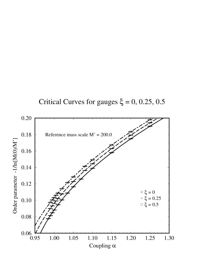
FIG. 4.: The critical curves for three choices of gauge parameter showing the existence of residual gauge-dependence in the Curtis-Pennington vertex. For the purposes of studying the chiral phase transition all solutions were renormalized with the choice, $m(\mu)=0$, with the renormalization point $\mu^{2}=10^{4}$. The order parameter is evaluated using an arbitrary reference mass scale choice of $M^{\prime}=200.0$. Diamonds ($\Diamond$) connected by the solid smooth curve, are order parameter values for the Landau gauge; pluses ($+$) connected by the dashed smooth curve, are values for $\xi=0.25$; and boxes ($\Box$) connected by the dot-dashed smooth curve, are values for $\xi=0.5$.

FIG. 5.: The finite renormalization $A(p^{2})$ and the mass function $M(p^{2})$ are shown for various choices of renormalization point. These results have coupling strength $\alpha=1.15$ and gauge parameter $\xi=0.50$. Each of these results corresponds to $M(p^{2})=400$ at $p^{2}=10^{8}$. Hence, $M(p^{2})$ is renormalization point independent and $A(p^{2})$ varies as described in Eq. (34).

FIG. 6.: Asymptotic mass scaling below critical coupling as a function of gauge, with $\alpha=0.5$, $\mu^{2}=10^{8}$, $m(\mu)=400$. The scaling applied to the masses uses the anomalous dimension found for the Landau guage, $\gamma_{m}(\xi=0)=1.716638$. the extracted anomalous dimensions for the other two curves are $\gamma_{m}(0.25)=1.713498$, and $\gamma_{m}(0.5)=1.711274$.

FIG. 7.: The finite renormalization $A(p^{2})$ and the mass function $M(p^{2})$ are shown with and without the gauge covariance correction. We see that the correction is a relatively small effect. These results have coupling strength $\alpha=1.15$, renormalization point $\mu^{2}=10^{8}$, renormalized mass $m(\mu)=400$, and gauge parameter $\xi=0.50$.

FIG. 8.: Detail of the node in the mass function $M(p^{2})$ for various gauge choices. These results have coupling strength $\alpha=1.15$, renormalization point $\mu^{2}=10^{8}$, and renormalized mass $m(\mu)=400$.

FIG. 9.: Absolute value of the dynamical mass, showing damped oscillations periodic in $\ln(p^{2})$. The solution shown has $\alpha=1.25$, $\xi=0.25$, and is renormalized with $\mu^{2}=10^{4}$, $m(\mu)=0$. The power-law fit, which runs tangent to the dynamical mass curve, is $C(p^{2}/\mu^{2})^{(\gamma_{m}/2)-1}$, with $C=4.394\times 10^{-2}$, $\gamma_{m}=1.115$.

TABLE I.: Renormalization constant $Z_{2}(\mu,\Lambda)$, bare masses $m_{0}(\Lambda)$, and mass renormalization $Z_{m}(\mu,\Lambda)$, as a function of UV cutoff for $\alpha=1.15$ in the Landau gauge ($\xi=0$). All solutions are with renormalization point $\mu^{2}=1.00\times 10^{8}$ and renormalized mass $m(\mu)=400.0$

$\Lambda^{2}$	$Z_{2}(\mu,\Lambda)$		$m_{0}(\Lambda)$		$Z_{m}(\mu,\Lambda)$
$1\times 10^{8}$	0.	9999135	2.	$306\times 10^{2}$	5.	$765\times 10^{-1}$
$1\times 10^{9}$	0.	9998483	5.	$358\times 10^{1}$	1.	$339\times 10^{-1}$
$1\times 10^{10}$	0.	9998468	4.	443	1.	$111\times 10^{-2}$
$1\times 10^{11}$	0.	9998469	-3.	932	-9.	$831\times 10^{-3}$
$1\times 10^{12}$	0.	9998469	-2.	847	-7.	$117\times 10^{-3}$
$1\times 10^{13}$	0.	9998469	-1.	182	-2.	$954\times 10^{-3}$
$1\times 10^{14}$	0.	9998469	-3.	$408\times 10^{-1}$	-8.	$520\times 10^{-4}$
$1\times 10^{15}$	0.	9998469	-5.	$390\times 10^{-2}$	-1.	$348\times 10^{-4}$
$1\times 10^{16}$	0.	9998469	1.	$043\times 10^{-2}$	2.	$607\times 10^{-5}$
$1\times 10^{17}$	0.	9998469	1.	$276\times 10^{-2}$	3.	$191\times 10^{-5}$
$1\times 10^{18}$	0.	9998469	6.	$171\times 10^{-3}$	1.	$543\times 10^{-5}$
$1\times 10^{19}$	0.	9998469	2.	$042\times 10^{-3}$	5.	$105\times 10^{-6}$

TABLE II.: Renormalization constant $Z_{2}(\mu,\Lambda)$, bare masses $m_{0}(\Lambda)$, and mass renormalization $Z_{m}(\mu,\Lambda)$, as a function of UV cutoff for $\alpha=1.15$ in the gauge with $\xi=0.25$. All solutions are with renormalization point $\mu^{2}=1.00\times 10^{8}$ and renormalized mass $m(\mu)=400.0$

$\Lambda^{2}$	$Z_{2}(\mu,\Lambda)$		$m_{0}(\Lambda)$		$Z_{m}(\mu,\Lambda)$
$1\times 10^{8}$	0.	999943	2.	$239\times 10^{2}$	5.	$598\times 10^{-1}$
$1\times 10^{9}$	0.	9486	4.	$918\times 10^{1}$	1.	$229\times 10^{-1}$
$1\times 10^{10}$	0.	8999	2.	034	5.	$085\times 10^{-3}$
$1\times 10^{11}$	0.	8537	-4.	898	-1.	$225\times 10^{-2}$
$1\times 10^{12}$	0.	8099	-3.	102	-7.	$756\times 10^{-3}$
$1\times 10^{13}$	0.	7683	-1.	193	-2.	$981\times 10^{-3}$
$1\times 10^{14}$	0.	7289	-3.	$059\times 10^{-1}$	-7.	$647\times 10^{-4}$
$1\times 10^{15}$	0.	6915	-2.	$886\times 10^{-2}$	-7.	$214\times 10^{-5}$
$1\times 10^{16}$	0.	6560	2.	$145\times 10^{-2}$	5.	$362\times 10^{-5}$
$1\times 10^{17}$	0.	6224	1.	$609\times 10^{-2}$	4.	$023\times 10^{-5}$
$1\times 10^{18}$	0.	5904	6.	$679\times 10^{-3}$	1.	$670\times 10^{-5}$

TABLE III.: Renormalization constant $Z_{2}(\mu,\Lambda)$, bare masses $m_{0}(\Lambda)$, and mass renormalization $Z_{m}(\mu,\Lambda)$, as a function of UV cutoff for $\alpha=1.15$ in the gauge with $\xi=0.5$. All solutions are with renormalization point $\mu^{2}=1.00\times 10^{8}$ and renormalized mass $m(\mu)=400.0$

$\Lambda^{2}$	$Z_{2}(\mu,\Lambda)$		$m_{0}(\Lambda)$		$Z_{m}(\mu,\Lambda)$
$1\times 10^{8}$	0.	99997	2.	$176\times 10^{2}$	5.	$441\times 10^{-1}$
$1\times 10^{9}$	0.	8999	4.	$513\times 10^{1}$	1.	$128\times 10^{-1}$
$1\times 10^{10}$	0.	8099	-1.	$455\times 10^{-1}$	-3.	$638\times 10^{-4}$
$1\times 10^{11}$	0.	7289	-5.	736	-1.	$434\times 10^{-2}$
$1\times 10^{12}$	0.	6560	-3.	299	-8.	$248\times 10^{-3}$
$1\times 10^{13}$	0.	5904	-1.	181	-2.	$954\times 10^{-3}$
$1\times 10^{14}$	0.	5314	-2.	$653\times 10^{-1}$	-6.	$632\times 10^{-4}$
$1\times 10^{15}$	0.	4783	-3.	$676\times 10^{-3}$	-9.	$190\times 10^{-6}$
$1\times 10^{16}$	0.	4304	3.	$151\times 10^{-2}$	7.	$877\times 10^{-5}$
$1\times 10^{17}$	0.	3874	1.	$870\times 10^{-2}$	4.	$674\times 10^{-5}$

TABLE IV.: Critical parameters for three choices of gauge, $\xi=0$, 0.25, and 0.50. These are extracted from nonlinear fits to the data in Fig. 4, using the form in Eq. (36).

Parameter	Landau ($\xi=0$)	$\xi=0.25$	$\xi=0.5$
$c$	$2.877\pm.027$	$2.858\pm.043$	$2.851\pm.055$
$\alpha_{c}$	$0.93307\pm.00023$	$0.92076\pm.00048$	$0.90946\pm.00071$
$\beta$	$0.512\pm.003$	$0.514\pm.005$	$0.516\pm.007$
$M$	$154.3\pm 5.2$	$148.5\pm 7.7$	$145.4\pm 9.4$
$\chi^{2}/{\rm DOF}$	0.0959	.0388	.0211

REFERENCES

- [1] C.D. Roberts and A.G. Williams, Dyson-Schwinger Equations and their Application to Hadronic Physics, in Progress in Particle and Nuclear Physics, Vol. 33 (Pergamon Press, Oxford, 1994), p. 477.
- [2] V. A. Miranskii, Dynamical Symmetry Breaking in Quantum Field Theories, (World Scientific, Singapore, 1993).
- [3] P. I. Fomin, V. P. Gusynin, V. A. Miransky and Yu. A. Sitenko, Riv. Nuovo Cim. 6, 1 (1983).
- [4] F.T. Hawes and A.G. Williams, Phys. Rev. D 51, 3081 (1995).
- [5] R. Haag and Th.A. Maris, Phys. Rev. 132, 2325 (1963); Th.A.J. Maris, V.E. Herscovitz and D. Jacob, Phys. Rev. Lett. 12, 313 (1964); T. Nonoyama and M. Tanabashi, Prog. Theor. Phys. 81, 209 (1989).
- [6] P. I. Fomin, V. P. Gusynin, and V. A. Miransky, Phys. Lett. 78B, 136 (1978).
- [7] V. A. Miransky, Sov. Phys. JETP 61 (5), 905 (1985).
- [8] V. A. Miransky, Nuovo Cimento 90A, 149 (1985).
- [9] P. E. L. Rakow, Nucl. Phys. B356, 27 (1991).
- [10] J.C. Ward, Phys. Rev. 78, 124 (1950); Y. Takahashi, Nuovo Cimento 6, 370 (1957).
- [11] K.-I. Aoki, M. Bando, T. Kugo, K. Hasebe and H. Nakatani, Prog. Theor. Phys. 81, 866 (1989).
- [12] D.C. Curtis and M.R. Pennington, Phys. Rev. D48, 4933 (1993).
- [13] K.-I. Kondo, Y. Kikukawa and H. Mino, Phys. Lett. 220B, 270 (1989).
- [14] D. Atkinson, P. W. Johnson and K. Stam, Phys. Lett. 201B, 105 (1988).
- [15] J.S. Ball and T.W. Chiu, Phys. Rev. D22, 2542 (1980); ibid., 2550 (1980).
- [16] J.E. King, Phys. Rev. D27, 1821 (1983).
- [17] P. Rembiesa, Phys. Rev. D41, 2009 (1990).
- [18] B. Haeri, Phys. Rev. D43, 2701 (1991).
- [19] D.C. Curtis and M.R. Pennington, Phys. Rev. D42, 4165 (1990).
- [20] D.C. Curtis and M.R. Pennington, Phys. Rev. D44, 536 (1991).
- [21] D.C. Curtis and M.R. Pennington, Phys. Rev. D46, 2663 (1992).
- [22] Z. Dong, H. Munczek, and C.D. Roberts, Phys. Lett. 333B, 536 (1994).
- [23] A. Bashir and M. R. Pennington, Phys. Rev. D 50, 7679 (1994).
- [24] A. Bashir and M. R. Pennington, Phys. Rev. D 53, 4694 (1996).
- [25] C.D. Roberts, Schwinger Dyson Equations: Dynamical chiral symmetry breaking and Confinement, in QCD Vacuum Structure, edited by H. M. Fried and B. Müller (World Scientific, Singapore, 1993).
- [26] A. Kizilersü, M. Reenders, and M. R. Pennington, Phys. Rev. D 52, 1242 (1995).
- [27] D. Atkinson, J.C.R. Bloch, V.P. Gusynin, M. R. Pennington, and M. Reenders, Phys. Lett. 329B, 117 (1994).
- [28] L. von Smekal, P. A. Amundsen, and R. Alkofer, Nucl. Phys. A529, 633 (1991); M. Becker, “Nichtperturbative Strukturuntersuchungen der QED mittels genäherter Schwinger-Dyson-Gleichungen in Dimensioneller Regularisierung,”, Ph.D. dissertation, W. W. U. Münster,1995.
- [29] C. Itzykson and J.B. Zuber, Quantum Field Theory, (McGraw-Hill, New York, 1980).
- [30] H. J. Rothe, Latticd Gauge Theories: an Introduction, (World Scientific, Singapore, 1992).
- [31] D. Atkinson and M.P. Fry, Nucl. Phys. B156, 301 (1979).
- [32] L. D. Landau and I. M. Khalatnikov, Sov. Phys. JETP 2, 69 (1956) [translation of Zhur. Eksptl. i Teoret. Fiz. 29, 89 (1955)]; K. Johnson and B. Zumino, Phys. Rev. Lett. 3, 351 (1959).
- [33] B. Holdom, Phys. Rev. Lett. 62, 997 (1989); (R) ibid. 63, 1889 (1989);
- [34] U. Mahanta, Phys. Lett. 225B, 181 (1989).
- [35] U. Mahanta, Phys. Rev. Lett. 62, 2349 (1989).
- [36] M. R. Frank and C. D. Roberts, Phys. Rev. D 53, 390 (1996).