LIGHT-CONE QUANTIZATION AND

HADRON STRUCTURE

Stanley J. Brodsky

Stanford Linear Accelerator Center

Stanford University, Stanford, California 94309

e-mail: sjbth@slac.stanford.edu

Talk presented at the

International Conference on Orbis Scientiae 1996

Miami Beach, Florida – January 25–28, 1996

1 INTRODUCTION

Quantum chromodynamics provides a fundamental description of hadronic and nuclear structure and dynamics in terms of elementary quark and gluon degrees of freedom. In practice, the direct application of QCD to reactions involving the structure of hadrons is extremely complex because of the interplay of nonperturbative effects such as color confinement and multi-quark coherence.

In this talk, I will discuss light-cone quantization and the light-cone Fock expansion as a tractable and consistent representation of relativistic many-body systems and bound states in quantum field theory. The Fock state representation in QCD includes all quantum fluctuations of the hadron wavefunction, including far off-shell configurations such as intrinsic strangeness and charm and, in the case of nuclei, hidden color. The Fock state components of the hadron with small transverse size, which dominate hard exclusive reactions, have small color dipole moments and thus diminished hadronic interactions. Thus QCD predicts minimal absorptive corrections, i.e., color transparency for quasi-elastic exclusive reactions in nuclear targets at large momentum transfer. In other applications, such as the calculation of the axial, magnetic, and quadrupole moments of light nuclei, the QCD relativistic Fock state description provides new insights which go well beyond the usual assumptions of traditional hadronic and nuclear physics.

2 QCD ON THE LIGHT CONE

The bound state structure of hadrons plays a critical role in virtually every area of particle physics phenomenology. For example, in the case of the nucleon form factors, pion electroproduction $ep\rightarrow e\pi^{+}n$, exclusive $B$ decays, and open charm photoproduction $\gamma p\rightarrow D\Lambda_{c}$, the cross sections depend not only on the nature of the quark currents, but also on the coupling of the quarks to the initial and final hadronic states. Exclusive decay amplitudes such as $B\rightarrow K^{*}\gamma$, processes which will be studied intensively at $B$ factories, depend not only on the underlying weak transitions between the quark flavors, but also the wavefunctions which describe how the $B$ and $K^{*}$ mesons are assembled in terms of their fundamental quark and gluon constituents. Unlike the leading twist structure functions measured in deep inelastic scattering, such exclusive channels are sensitive to the structure of the hadrons at the amplitude level and to the coherence between the contributions of the various quark currents and multi-parton amplitudes.

The analytic problem of describing QCD bound states is compounded not only by the physics of confinement, but also by the fact that the wavefunction of a composite of relativistic constituents has to describe systems of an arbitrary number of quanta with arbitrary momenta and helicities. The conventional Fock state expansion based on equal-time quantization quickly becomes intractable because of the complexity of the vacuum in a relativistic quantum field theory. Furthermore, boosting such a wavefunction from the hadron’s rest frame to a moving frame is as complex a problem as solving the bound state problem itself. The Bethe-Salpeter bound state formalism, although manifestly covariant, requires an infinite number of irreducible kernels to compute the matrix element of the electromagnetic current even in the limit where one constituent is heavy.

Light-cone quantization (LCQ) is formally similar to equal-time quantization (ETQ) apart from the choice of initial-value surface. In ETQ one chooses a surface of constant time in some Lorentz frame on which to specify initial values for the fields. In quantum field theory this corresponds to specifying commutation relations among the fields at some fixed time. The equations of motion, or the Heisenberg equations in the quantum theory, are then used to evolve this initial data in time, filling out the solution at all spacetime points.

In LCQ one chooses instead a hyperplane tangent to the light cone—properly called a null plane or light front—as the initial-value surface. To be specific, we introduce LC coordinates

$$x^{\pm}\equiv x^{0}\pm x^{3}$$ (1)

(and analogously for all other four-vectors). The selection of the 3 direction in this definition is of course arbitrary. In terms of LC coordinates, a contraction of four-vectors decomposes as

$$p\cdot x=\frac{1}{2}(p^{+}x^{-}+p^{-}x^{+})-p_{\perp}\cdot x_{\perp}\;,$$ (2)

from which we see that the momentum “conjugate” to $x^{+}$ is $p^{-}$. Thus the operator $P^{-}$ plays the role of the Hamiltonian in this scheme, generating evolution in $x^{+}$ according to an equation of the form (in the Heisenberg picture)

$$[\phi,P^{-}]=2i\,\frac{\partial\phi}{\partial x^{+}}\;.$$ (3)

As was first shown by Dirac [1], seven of the ten Poincaré generators become kinematical on the LC , the maximum number possible. The most important point is that these include Lorentz boosts. Thus in the LC representation boosting states is trivial—the generators are diagonal in the Fock representation so that computing the necessary exponential is simple. One result of this is that the LC theory can be formulated in a manifestly frame-independent way, yielding wavefunctions that depend only on momentum fractions and which are valid in any Lorentz frame. This advantage is somewhat compensated for, however, in that certain rotations become nontrivial in LCQ. Thus rotational invariance will not be manifest in this approach.

Another advantage of going to the LC is even more striking: the vacuum state seems to be much simpler in the LC representation than in ETQ. Note that the longitudinal momentum $p^{+}$ is conserved in interactions. For particles, however, this quantity is strictly positive,

$$p^{+}=\left(p_{3}^{2}+p_{\perp}^{2}+m^{2}\right)^{\frac{1}{2}}+p^{3}>0\;.$$ (4)

Thus the Fock vacuum is the only state in the theory with $p^{+}=0$, and so it must be an exact eigenstate of the full interacting Hamiltonian. Stated more dramatically, the Fock vacuum in the LC representation is the physical vacuum state. To the extent that this is really true, it represents a tremendous simplification, as attempts to compute the spectrum and wavefunctions of some physical state are not complicated by the need to recreate a ground state in which processes occur at unrelated locations and energy scales. Furthermore, it immediately gives a constituent picture; all the quanta in a hadron’s wavefunction are directly connected to that hadron. This allows a precise definition of the partonic content of hadrons and makes interpretation of the LC wavefunctions unambiguous. It also raises the question, however, of whether LC field theory can be equivalent in all respects to field theories quantized at equal times, where nonperturbative effects often lead to nontrivial vacuum structure. In QCD, for example, there is an infinity of possible vacua labelled by a continuous parameter $\theta$, and chiral symmetry is spontaneously broken. The question is how it is possible to identify and incorporate such phenomena into a formalism in which the vacuum state is apparently simple.

The description of relativistic composite systems using light-cone quantization [1] thus appears to be remarkably simple. The Heisenberg problem for QCD can be written in the form

$$H_{LC}|H\rangle=M_{H}^{2}|H\rangle\;,$$ (5)

where $H_{LC}=P^{+}P^{-}-P_{\perp}^{2}$ is the mass operator. The operator $P^{-}=P^{0}-P^{3}$ is the generator of translations in the light-cone time $x^{+}=x^{0}+x^{3}.$ The quantities $P^{+}=P^{0}+P^{3}$ and $P_{\perp}$ play the role of the conserved three-momentum. Each hadronic eigenstate $|H\rangle$ of the QCD light-cone Hamiltonian can be expanded on the complete set of eigenstates $\{|n\rangle\}$ of the free Hamiltonian which have the same global quantum numbers: $|H\rangle=\sum\psi^{H}_{n}(x_{i},k_{\perp i},\lambda_{i})|n\rangle.$ In the case of the proton, the Fock expansion begins with the color singlet state $|uud\rangle$ of free quarks, and continues with $|uudg\rangle$ and the other quark and gluon states that span the degrees of freedom of the proton in QCD. The Fock states $\{|n\rangle\}$ are built on the free vacuum by applying the free light-cone creation operators. The summation is over all momenta $(x_{i},k_{\perp i})$ and helicities $\lambda_{i}$ satisfying momentum conservation $\sum^{n}_{i}x_{i}=1$ and $\sum^{n}_{i}k_{\perp i}=0$ and conservation of the projection $J^{3}$ of angular momentum.

The wavefunction $\psi^{p}_{n}(x_{i},k_{\perp i},\lambda_{i})$ describes the probability amplitude that a proton of momentum $P^{+}=P^{0}+P^{3}$ and transverse momentum $P_{\perp}$ consists of $n$ quarks and gluons with helicities $\lambda_{i}$ and physical momenta $p^{+}_{i}=x_{i}P^{+}$ and $p_{\perp i}=x_{i}P_{\perp}+k_{\perp i}$. The wavefunctions $\{\psi^{p}_{n}(x_{i},k_{\perp i},\lambda_{i})\},n=3,\dots$ thus describe the proton in an arbitrary moving frame. The variables $(x_{i},k_{\perp i})$ are internal relative momentum coordinates. The fractions $x_{i}=p^{+}_{i}/P^{+}=(p^{0}_{i}+p^{3}_{i})/(P^{0}+P^{3})$, $0<x_{i}<1$, are the boost-invariant light-cone momentum fractions; $y_{i}=\log x_{i}$ is the difference between the rapidity of the constituent $i$ and the rapidity of the parent hadron. The appearance of relative coordinates is connected to the simplicity of performing Lorentz boosts in the light-cone framework. This is another major advantage of the light-cone representation.

The spectra of hadrons and nuclei as well as their scattering states can be identified with the set of eigenvalues of the light-cone Hamiltonian $H_{LC}$ for QCD. Particle number is generally not conserved in a relativistic quantum field theory, so that each eigenstate is represented as a sum over Fock states of arbitrary particle number. Thus in QCD each hadron is expanded as second-quantized sums over fluctuations of color-singlet quark and gluon states of different momenta and number. The coefficients of these fluctuations are the light-cone wavefunctions $\psi_{n}(x_{i},k_{\perp i},\lambda_{i}).$ The invariant mass ${\cal M}$ of the partons in a given $n$-particle Fock state can be written in the elegant form

$${\cal M}^{2}=\sum_{i=1}^{n}\frac{k_{\perp i}^{2}+m^{2}}{x_{i}}\;.$$ (6)

The dominant configurations in the wavefunction are generally those with minimum values of ${\cal M}^{2}$. Note that, except for the case where $m_{i}=0$ and $k_{\perp i}=0$, the limit $x_{i}\rightarrow 0$ is an ultraviolet limit, i.e., it corresponds to particles moving with infinite momentum in the negative $z$ direction: $k^{z}_{i}\rightarrow-k^{0}_{i}\rightarrow-\infty.$ The light-cone wavefunctions encode the properties of the hadronic wavefunctions in terms of their quark and gluon degrees of freedom, and thus all hadronic properties can be derived from them. The natural gauge for light-cone Hamiltonian theories is the light-cone gauge $A^{+}=0$. In this physical gauge the gluons have only two physical transverse degrees of freedom, and thus it is well matched to perturbative QCD calculations.

Since QCD is a relativistic quantum field theory, determining the wavefunction of a hadron is an extraordinarily complex nonperturbative relativistic many-body problem. In principle it is possible to compute the light-cone wavefunctions by diagonalizing the QCD light-cone Hamiltonian on the free Hamiltonian basis. In the case of QCD in one space and one time dimensions, the application of discretized light-cone quantization (DLCQ) [2] provides complete solutions of the theory, including the entire spectrum of mesons, baryons, and nuclei, and their wavefunctions [3, 4]. In the DLCQ method, one simply diagonalizes the light-cone Hamiltonian for QCD on a discretized Fock state basis. The DLCQ solutions can be obtained for arbitrary parameters including the number of flavors and colors and quark masses. More recently, DLCQ has been applied to new variants of QCD₁₊₁ with quarks in the adjoint representation, thus obtaining color-singlet eigenstates analogous to gluonium states [5].

The extension of this program to physical theories in 3+1 dimensions is a formidable computational task because of the much larger number of degrees of freedom; however, progress is being made. Analyses of the spectrum and light-cone wavefunctions of positronium in QED₃₊₁ are given elsewhere [6]. Hiller, Okamoto and I [7] have been pursuing a nonperturbative calculation of the lepton anomalous moment in QED using the DLCQ method. Burkardt has recently solved scalar theories with transverse dimensions by combining a Monte Carlo lattice method with DLCQ [8]. Also of interest is recent work of Hollenberg and Witte [9], who have shown how Lanczos tri-diagonalization can be combined with a plaquette expansion to obtain an analytic extrapolation of a physical system to infinite volume.

There has also been considerable work on the truncations required to reduce the space of states to a manageable level [10, 11, 12]. The natural language for this discussion is that of the renormalization group, with the goal being to understand the kinds of effective interactions that occur when states are removed, either by cutoffs of some kind or by an explicit Tamm-Dancoff truncation. Solutions of the resulting effective Hamiltonians can then be obtained by various means, for example using DLCQ or basis function techniques. Some calculations of the spectrum of heavy quarkonia in this approach have recently been reported [13].

One of the remarkable simplicities of the LC formalism is the fact that one can write down exact expressions for the spacelike electromagnetic form factors $\langle P+Q|J^{+}|P\rangle$ of any hadrons for any initial or final state helicity. At a fixed light-cone time, the exact Heisenberg current can be identified with the free current $j^{+}$. It is convenient to choose the frame in which $q^{+}=0$ so that $q_{\perp}^{2}$ is $Q^{2}=-q_{\mu}^{2}.$ Since the quark current $j^{+}$ has simple matrix elements between free Fock states, each form factor for a given helicity transition $\lambda\rightarrow\lambda^{\prime}$ can be evaluated from simple overlap integrals of the light-cone wavefunctions [14, 15]:

$$F_{\lambda^{\prime},\lambda}(Q^{2})=\sum_{n}\int\prod d^{2}k_{\perp i}\int{\prod dx_{i}}\overline{\psi}_{n,\lambda^{\prime}}(x_{i},k^{\prime}_{\perp i},\lambda_{i})\psi_{n,\lambda}(x_{i},k_{\perp i},\lambda_{i})\;,$$ (7)

where the integrations are over the unconstrained relative coordinates. The internal transverse momenta of the final state wavefunction are $k^{\prime}_{\perp}=k_{\perp}+(1-x)q_{\perp}$ for the struck quark and $k_{\perp}^{\prime}=k_{\perp}-xq_{\perp}$ for the spectator quarks. Thus given the light-cone wavefunctions $\{\psi_{n}(x_{i},k_{\perp_{i}},\lambda_{i})\}$ one can compute the electromagnetic and weak form factors from a simple overlap of light-cone wavefunctions, summed over all Fock states [14, 15]. For spacelike momentum transfer only diagonal matrix elements in particle number $n^{\prime}=n$ are needed. In contrast, in the equal-time theory one must also consider off-diagonal matrix elements and fluctuations due to particle creation and annihilation in the vacuum. In the nonrelativistic limit one can make contact with the usual formulae for form factors in Schrödinger many-body theory.

The structure functions of a hadron can be computed from the square integral of its LC wavefunctions [16]. For example, the quark distribution measured in deep inelastic scattering at a given resolution $Q^{2}$ is

$$q(x_{Bj},Q^{2})=\sum_{n}\int^{k_{\perp}^{2}<Q^{2}}\prod d^{2}k_{\perp i}\int{\prod dx_{i}}|\psi_{n}(x_{i},k_{\perp i},\lambda_{i})|^{2}\delta(x_{q}=x_{Bj})\;,$$ (8)

where the struck quark is evaluated with its light-cone fraction equal to the Bjorken variable: $x_{q}=x_{Bj}=Q^{2}/2p\cdot q.$ A summation over all contributing Fock states is required to evaluate the form factors and structure functions. Thus the hadron and nuclear structure functions are the probability distributions constructed from integrals over the absolute squares $|\psi_{n}|^{2}$, summed over $n.$ In the far off-shell domain of large parton virtuality, one can use perturbative QCD to derive the asymptotic fall-off of the Fock amplitudes, which then in turn leads to the QCD evolution equations for distribution amplitudes and structure functions. More generally, one can prove factorization theorems for exclusive and inclusive reactions which separate the hard and soft momentum transfer regimes, thus obtaining rigorous predictions for the leading power behavior contributions to large momentum transfer cross sections. One can also compute the far off-shell amplitudes within the light-cone wavefunctions where heavy quark pairs appear in the Fock states. Such states persist over a time $\tau\simeq P^{+}/{\cal M}^{2}$ until they are materialized in the hadron collisions. As we shall discuss below, this leads to a number of novel effects in the hadroproduction of heavy quark hadronic states [17].

Although we are still far from solving QCD explicitly, a number of properties of the light-cone wavefunctions of the hadrons are known from both phenomenology and the basic properties of QCD. For example, the endpoint behavior of light-cone wavefunctions and structure functions can be determined from perturbative arguments and Regge arguments. Applications are presented elsewhere [18]. There are also correspondence principles. For example, for heavy quarks in the nonrelativistic limit, the light-cone formalism reduces to conventional many-body Schrödinger theory. On the other hand, one can also build effective three-quark models which encode the static properties of relativistic baryons.

3 SOLVING NONPERTURBATIVE QUANTUM FIELD THEORY USING LCQ

A large number of studies have been performed of model field theories in the LC framework. This approach has been remarkably successful in a range of toy models in 1+1 dimensions: Yukawa theory [19], the Schwinger model (for both massless and massive fermions) [20, 21], $\phi^{4}$ theory [22], QCD with various types of matter [3, 4, 5, 23, 24], and the sine-Gordon model [25]. It has also been applied with promising results to theories in 3+1 dimensions, in particular QED [6] and Yukawa theory [26]. In all cases agreement was found between the LC calculations and results obtained by more conventional approaches, for example, lattice gauge theory. In many cases the physics of spontaneous symmetry breaking and vacuum structure of the equal-time theory is represented by the physics of zero modes in LCQ [27].

3.1 QCD₁₊₁ with Fundamental Matter

This theory was originally considered by ’t Hooft in the limit of large $N_{c}$ [28]. Later Burkardt [3], and Hornbostel, Pauli and I [4], gave essentially complete numerical solutions of the theory for finite $N_{c}$, obtaining the spectra of baryons, mesons, and nucleons and their wavefunctions. The results are consistent with the few other calculations available for comparison, and are generally much more efficiently obtained. In particular, the mass of the lowest meson agrees to within numerical accuracy with lattice Hamiltonian results [29]. For $N_{c}=4$ this mass is close to that obtained by ’t Hooft in the $N_{c}\rightarrow\infty$ limit [28]. Finally, the ratio of baryon to meson mass as a function of $N_{c}$ agrees with the strong-coupling results of Date, Frishman and Sonnenschein [30].

In addition to the spectrum, of course, one obtains the wavefunctions. These allow direct computation of, e.g., structure functions. As an example, Fig. 1 shows the valence contribution to the structure function for an SU(3) baryon, for two values of the dimensionless coupling $m/g$. As expected, for weak coupling the distribution is peaked near $x=1/3$, reflecting that the baryon momentum is shared essentially equally among its constituents. For comparison, the contributions from Fock states with one and two additional $q\overline{q}$ pairs are shown in Fig. 2. Note that the amplitudes for these higher Fock components are quite small relative to the valence configuration. The lightest hadrons are nearly always dominated by the valence Fock state in these super-renormalizable models; higher Fock wavefunctions are typically suppressed by factors of 100 or more. Thus the light-cone quarks are much more like constituent quarks in these theories than equal-time quarks would be. As discussed above, in an equal-time formulation even the vacuum state would be an infinite superposition of Fock states. Identifying constituents in this case, three of which could account for most of the structure of a baryon, would be quite difficult.

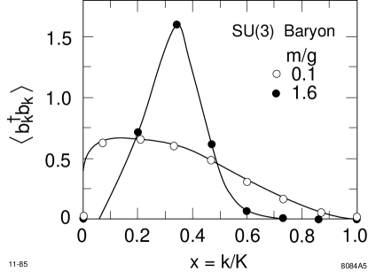
Figure 1: Valence contribution to the baryon structure function in QCD₁₊₁, as a function of the light-cone longitudinal momentum fraction. The gauge group is SU(3), $m$ is the quark mass, and $g$ is the gauge coupling [4].

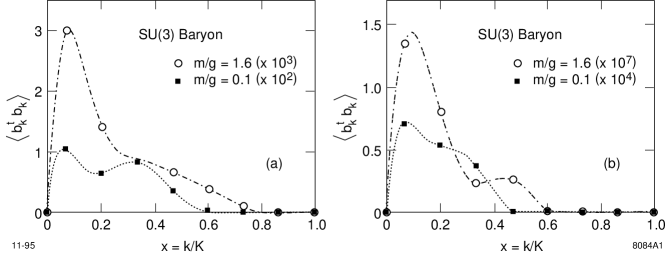
Figure 2: Contributions to the baryon structure function from higher Fock components: (a) valence plus one additional $q\overline{q}$ pair; (b) valence plus two additional $q\overline{q}$ pairs [4].

3.2 Collinear QCD

QCD can be simplified in a dramatic way by eliminating all interactions which involve nonzero transverse momentum. The trigluon interaction is eliminated but the four-gluon and helicity flip $q\overline{q}g$ vertices still survive. In this simplified “reduced” or “collinear” theory, one still has all of the degrees of freedom of QCD(3+1) including transversely polarized color adjoint gluons, but the theory is effectively a one-space, one-time theory which can be solved using discretized light-cone quantization. Recently Antonuccio and Dalley [24] have presented a comprehensive DLCQ analysis of collinear QCD, obtaining the full physical spectrum of both quarkonium and gluonium states. One also obtains the complete LC Fock wavefunctions for each state of the spectrum. An important feature of this analysis is the restoration of complete rotational symmetry through the degeneracy of states of the rest frame angular momentum. In fact as emphasized by Burkardt [31], parity and rotational invariance can be restored if one separately renormalizes the mass that appears in the helicity-flip $q\overline{q}g$ vertices and the light-cone kinetic energy.

Antonuccio and Dalley [24] have also derived ladder relations which connect the endpoint $x_{q}\to 0$ behavior of Fock states with $n$ gluons to the Fock state wavefunction with $n-1$ gluons, relations which follow most by imposing the condition that the $k^{+}=0$ mode of the constraint equations vanishes on physical states. An important condition for a bound state wavefunction is that gauge invariant quanta have should finite kinetic energy in a bound state, just as the square of the “mechanical velocity” operator ${\vec{v}}^{2}=(\vec{p}-e\vec{A})^{2}$ has finite expectation value in nonrelativistic electrodynamics. Such a condition automatically connects Fock states of different particle number. Thus the ladder relations should be generalizable to the full $3+1$ theory by requiring that the gauge-extended light-cone kinetic energy operator have finite expectation value.

4 EXCLUSIVE PROCESSES AND LIGHT-CONE QUANTIZATION

A central focus of future QCD studies will be hadron physics at the amplitude level. Exclusive reactions such as pion electroproduction $\gamma^{*}p\rightarrow np$ are more subtle to analyze than deep inelastic lepton scattering and other leading-twist inclusive reactions since they require the consideration of coherent QCD effects. Nevertheless, there is an extraordinary simplification: In any exclusive reaction where the hadrons are forced to absorb large momentum transfer $Q$, one can isolate the nonperturbative long-distance physics associated with hadron structure from the short-distance quark-gluon hard scattering amplitudes responsible for the dynamical reaction. In essence, to leading order in $1/Q,$ each exclusive reaction $AB\rightarrow CD$ factorizes in the form:

$$T_{AB\rightarrow CD}=\int^{1}_{0}\Pi dx_{i}\phi^{\dagger}_{D}(x_{i},Q)\phi^{\dagger}_{C}(x_{i},Q)\phi_{A}(x_{i},Q)\phi_{B}(x_{i},Q)T_{\rm quark}\;,$$ (9)

where $\phi_{A}(x_{i},Q)=\int^{k_{\perp}^{2}<Q^{2}}\prod d^{2}k_{\perp i}{\prod dx_{i}}\psi_{\rm valence}(x_{i},k_{\perp i},\lambda_{i})$ is the process-independent distribution amplitude—the light-cone wavefunction which describes the coupling of hadron $A$ to its valence quark with longitudinal light-cone momentum fractions $0<x_{i}<1$ at impact separation $b={\cal O}(1/Q)$—and $T_{\rm quark}$ is the amplitude describing the hard scattering of the quarks collinear with the hadrons in the initial state to the quarks which are collinear with the hadrons in the final state. Since the propagators and loop momenta in the hard scattering amplitude $T_{\rm quark}$ are of order $Q$, it can be computed perturbatively in QCD. The dimensional counting rules [32] for form factors and fixed CM scattering angle processes follow from the nominal power-law fall off of $T_{\rm quark}$. The scattering of the quarks all occurs at short distances; thus the hard scattering amplitude only couples to the valence-quarks the hadrons when they are at small relative impact parameter. Remarkably, there are no initial state or final state interaction corrections to factorization to leading order in $1/Q$ because of color coherence; final state color interactions are suppressed. This feature not only insures the validity of the factorization theorem for exclusive processes in QCD, but it also leads to the novel effect of “color transparency” in quasi-elastic nuclear reactions [33, 34].

An essential element of the factorization of high momentum transfer exclusive reactions is universality, i.e., the distribution amplitudes $\phi_{A}(x_{i},Q)$ are unique wavefunctions specific to each hadron [35]. The distribution amplitudes obey evolution equations and renormalization group equations [16] which can be derived through the light-cone equations of motion or the operator product expansion. Thus the same wavefunction that controls the meson form factors also controls the formation of the mesons in exclusive decay amplitudes of $B$ mesons such as $B\rightarrow\pi\pi$ at the comparable momenta.

5 THE EFFECTIVE CHARGE $\alpha_{V}(Q^{2})$ AND LIGHT-CONE QUANTIZATION

The heavy quark potential plays a central role in QCD, not only in determining the spectrum and wavefunctions of heavy quarkonium, but also in providing a physical definition of the running coupling for QCD. The heavy quark potential $V(Q^{2})$ is defined as the two-particle irreducible amplitude controlling the scattering of two infinitely heavy test quarks $Q\overline{Q}$ in an overall color-singlet state. Here $Q^{2}=-q^{2}={\vec{q}}^{2}$ is the momentum transfer. The effective charge $\alpha_{V}(Q^{2})$ is then defined through the relation $V(Q^{2})=-4\pi C_{F}\alpha_{V}(Q^{2})/Q^{2}$ where $C_{F}=(N_{c}^{2}-1)/2N_{c}=4/3.$ The running coupling $\alpha_{V}(Q^{2})$ satisfies the usual renormalization group equation, where the first two terms $\beta_{0}$ and $\beta_{1}$ in the perturbation series are universal coefficients independent of the renormalization scheme or choice of effective charge. Thus $\alpha_{V}$ provides a physical expansion parameter for perturbative expansions in PQCD.

By definition, all quark and gluon vacuum polarization contributions are summed into $\alpha_{V}$; the scale $Q$ of $\alpha_{V}(Q^{2})$ that appears in perturbative expansions is thus fixed by the requirement that no terms involving the QCD $\beta$-function appear in the coefficients. Thus expansions in $\alpha_{V}$ are identical to that of conformally invariant QCD. This argument is the basis for BLM scale-fixing [36] and commensurate scale relations [37], which relate physical observables together without renormalization scale, renormalization scheme, or other ambiguities arising from theoretical conventions.

There has recently been remarkable progress [38] in determining the running coupling $\alpha_{V}(Q^{2})$ from heavy quark lattice gauge theory using as input a measured level splitting in the $\Upsilon$ spectrum. The heavy quark potential can also be determined in a direct way from experiment by measuring $e^{+}e^{-}\to c\overline{c}$ and $e^{+}e^{-}\to b\overline{b}$ at threshold [39]. The cross section at threshold is strongly modified by the QCD Sommerfeld rescattering of the heavy quarks through their Coulombic gluon interactions. The amplitude near threshold is modified by a factor $S(\beta,Q^{2})=x/(1-\exp(-x))$, where $x=C_{F}\alpha_{V}(Q^{2})/\beta$ and $\beta=\sqrt{1-4m_{Q}^{2})/s}$ is the relative velocity between the produced quark and heavy quark. The scale $Q$ reflects the mean exchanged momentum transfer in the Coulomb rescattering. For example, the angular distribution for $e^{+}e^{-}\to Q\overline{Q}$ has the form $1+A(\beta)\cos^{2}\theta_{\rm cm}.$ The anisotropy predicted in QCD for small $\beta$ is then $A={\widetilde{A}}/(1+{\widetilde{A}})$, where

$${\widetilde{A}}=\frac{\beta^{2}}{2}\frac{S(\beta,4m_{Q}^{2}\beta^{2}/e)}{S(\beta,4m_{Q}^{2}\beta^{2})}\frac{1-\frac{4}{\pi}\alpha_{V}(m_{Q}^{2}\exp 7/6)}{1-\frac{16}{3\pi}\alpha_{V}(m_{Q}^{2}\exp 3/4)}.$$ (10)

The last factor is due to hard virtual radiative corrections. The anisotropy in $e^{+}e^{-}\to Q\overline{Q}$ will be reflected in the angular distribution of the heavy mesons produced in the corresponding exclusive channels.

The renormalization scheme corresponding to the choice of $\alpha_{V}$ as the coupling is the natural one for analyzing QCD in the light-cone formalism, since it automatically sums all vacuum polarization contributions into the coupling. For example, once one knows the form of $\alpha_{V}(Q^{2}),$ it can be used directly in the light-cone formalism as a means to compute the wavefunctions and spectrum of heavy quark systems. The effects of the light quarks and higher Fock state gluons that renormalize the coupling are already contained in $\alpha_{V}.$

The same coupling can also be used for computing the hard scattering amplitudes that control large momentum transfer exclusive reactions and heavy hadron weak decays. Thus when evaluating $T_{\rm quark}$ the scale appropriate for each appearance of the running coupling $\alpha_{V}$ is the momentum transfer of the corresponding exchanged gluon [40]. This prescription agrees with the BLM procedure. The connection between $\alpha_{V}$ and the usual $\alpha_{\overline{MS}}$ scheme is described elsewhere [37].

6 THE PHYSICS OF LIGHT-CONE FOCK STATES

The light-cone formalism provides the theoretical framework which allows for a hadron to exist in various Fock configurations. For example, quarkonium states not only have valence $Q\overline{Q}$ components but they also contain $Q\overline{Q}g$ and $Q\overline{Q}gg$ states in which the quark pair is in a color-octet configuration. Similarly, nuclear LC wave functions contain components in which the quarks are not in color-singlet nucleon sub-clusters. In some processes, such as large momentum transfer exclusive reactions, only the valence color-singlet Fock state of the scattering hadrons with small inter-quark impact separation $b_{\perp}={\cal O}(1/Q)$ can couple to the hard scattering amplitude. In reactions in which large numbers of particles are produced, the higher Fock components of the LC wavefunction will be emphasized. The higher particle number Fock states of a hadron containing heavy quarks can be diffractively excited, leading to heavy hadron production in the high momentum fragmentation region of the projectile. In some cases the projectile’s valence quarks can coalesce with quarks produced in the collision, producing unusual leading-particle correlations. Thus the multi-particle nature of the LC wavefunction can manifest itself in a number of novel ways. For example:

6.1 Color Transparency

QCD predicts that the Fock components of a hadron with a small color dipole moment can pass through nuclear matter without interactions [33, 34]. Thus in the case of large momentum transfer reactions, where only small-size valence Fock state configurations enter the hard scattering amplitude, both the initial and final state interactions of the hadron states become negligible.

Color Transparency can be measured though the nuclear dependence of totally diffractive vector meson production $d\sigma/dt(\gamma^{*}A\to VA).$ For large photon virtualities (or for heavy vector quarkonium), the small color dipole moment of the vector system implies minimal absorption. Thus, remarkably, QCD predicts that the forward amplitude $\gamma^{*}A\to VA$ at $t\to 0$ is nearly linear in $A$. One is also sensitive to corrections from the nonlinear $A$-dependence of the nearly forward matrix element that couples two gluons to the nucleus, which is closely related to the nuclear dependence of the gluon structure function of the nucleus [41].

The integral of the diffractive cross section over the forward peak is thus predicted to scale approximately as $A^{2}/R_{A}^{2}\sim A^{4/3}.$ Evidence for color transparency in quasi-elastic $\rho$ leptoproduction $\gamma^{*}A\to\rho^{0}N(A-1)$ has recently been reported by the E665 experiment at Fermilab [42] for both nuclear coherent and incoherent reactions. A test could also be carried out at very small $t_{\rm min}$ at HERA, and would provide a striking test of QCD in exclusive nuclear reactions. There is also evidence for QCD “color transparency” in quasi-elastic $pp$ scattering in nuclei [43]. In contrast to color transparency, Fock states with large-scale color configurations interact strongly and with high particle number production [44].

6.2 Hidden Color

The deuteron form factor at high $Q^{2}$ is sensitive to wavefunction configurations where all six quarks overlap within an impact separation $b_{\perp i}<{\cal O}(1/Q);$ the leading power-law fall off predicted by QCD is $F_{d}(Q^{2})=f(\alpha_{s}(Q^{2}))/(Q^{2})^{5}$, where, asymptotically, $f(\alpha_{s}(Q^{2}))\propto\alpha_{s}(Q^{2})^{5+2\gamma}$. [45] The derivation of the evolution equation for the deuteron distribution amplitude and its leading anomalous dimension $\gamma$ is given elsewhere [46]. In general, the six-quark wavefunction of a deuteron is a mixture of five different color-singlet states. The dominant color configuration at large distances corresponds to the usual proton-neutron bound state. However at small impact space separation, all five Fock color-singlet components eventually acquire equal weight, i.e., the deuteron wavefunction evolves to 80% “hidden color.” The relatively large normalization of the deuteron form factor observed at large $Q^{2}$ points to sizable hidden color contributions [47].

6.3 Spin-Spin Correlations in Nucleon-Nucleon Scattering and the Charm Threshold

One of the most striking anomalies in elastic proton-proton scattering is the large spin correlation $A_{NN}$ observed at large angles [48]. At $\sqrt{s}\simeq 5$ GeV, the rate for scattering with incident proton spins parallel and normal to the scattering plane is four times larger than that for scattering with anti-parallel polarization. This strong polarization correlation can be attributed to the onset of charm production in the intermediate state at this energy [49]. The intermediate state $|uuduudc\overline{c}\rangle$ has odd intrinsic parity and couples to the $J=S=1$ initial state, thus strongly enhancing scattering when the incident projectile and target protons have their spins parallel and normal to the scattering plane. The charm threshold can also explain the anomalous change in color transparency observed at the same energy in quasi-elastic $pp$ scattering. A crucial test is the observation of open charm production near threshold with a cross section of order of $1\mu$b.

6.4 Anomalous Decays of the $J/\psi$

The dominant two-body hadronic decay channel of the $J/\psi$ is $J/\psi\rightarrow\rho\pi$, even though such vector-pseudoscalar final states are forbidden in leading order by helicity conservation in perturbative QCD [50]. The $\psi^{\prime}$, on the other hand, appears to respect PQCD. The $J/\psi$ anomaly may signal mixing with vector gluonia or other exotica [50].

6.5 The QCD Van Der Waals Potential and Nuclear Bound Quarkonium

The simplest manifestation of the nuclear force is the interaction between two heavy quarkonium states, such as the $\Upsilon(b\overline{b})$ and the $J/\psi(c\overline{c})$. Since there are no valence quarks in common, the dominant color-singlet interaction arises simply from the exchange of two or more gluons. In principle, one could measure the interactions of such systems by producing pairs of quarkonia in high energy hadron collisions. The same fundamental QCD van der Waals potential also dominates the interactions of heavy quarkonia with ordinary hadrons and nuclei. The small size of the $Q\overline{Q}$ bound state relative to the much larger hadron allows a systematic expansion of the gluonic potential using the operator product expansion [51]. The coupling of the scalar part of the interaction to large-size hadrons is rigorously normalized to the mass of the state via the trace anomaly. This scalar attractive potential dominates the interactions at low relative velocity. In this way one establishes that the nuclear force between heavy quarkonia and ordinary nuclei is attractive and sufficiently strong to produce nuclear-bound quarkonium [51, 52].

6.6 Anomalous Quarkonium Production at the Tevatron

Strong discrepancies between conventional QCD predictions and experiment of a factor of 30 or more have recently been observed for $\psi$, $\psi^{\prime}$, and $\Upsilon$ production at large $p_{T}$ in high energy $p\overline{p}$ collisions at the Tevatron [53]. Braaten and Fleming [54] have suggested that the surplus of charmonium production is due to the enhanced fragmentation of gluon jets coupling to the octet $c\overline{c}$ components in higher Fock states $|c\overline{c}gg\rangle$ of the charmonium wavefunction. Such Fock states are required for a consistent treatment of the radiative corrections to the hadronic decay of $P$-waves in QCD [55].

7 INTRINSIC HEAVY QUARK CONTRIBUTIONS IN HADRONIC WAVEFUNCTIONS

It is important to distinguish two distinct types of quark and gluon contributions to the nucleon sea measured in deep inelastic lepton-nucleon scattering: “extrinsic” and “intrinsic” [56]. The extrinsic sea quarks and gluons are created as part of the lepton-scattering interaction and thus exist over a very short time $\Delta\tau\sim 1/Q$. These factorizable contributions can be systematically derived from the QCD hard bremsstrahlung and pair-production (gluon-splitting) subprocesses characteristic of leading twist perturbative QCD evolution. In contrast, the intrinsic sea quarks and gluons are multiconnected to the valence quarks and exist over a relatively long lifetime within the nucleon bound state. Thus the intrinsic $q\overline{q}$ pairs can arrange themselves together with the valence quarks of the target nucleon into the most energetically-favored meson-baryon fluctuations.

In conventional studies of the “sea” quark distributions, it is usually assumed that, aside from the effects due to antisymmetrization, the quark and antiquark sea contributions have the same momentum and helicity distributions. However, the ansatz of identical quark and antiquark sea contributions has never been justified, either theoretically or empirically. Obviously the sea distributions which arise directly from gluon splitting in leading twist are necessarily CP-invariant; i.e., they are symmetric under quark and antiquark interchange. However, the initial distributions which provide the boundary conditions for QCD evolution need not be symmetric since the nucleon state is itself not CP-invariant. Only the global quantum numbers of the nucleon must be conserved. The intrinsic sources of strange (and charm) quarks reflect the wavefunction structure of the bound state itself; accordingly, such distributions would not be expected to be CP symmetric. Thus the strange/anti-strange asymmetry of nucleon structure functions provides a direct window into the quantum bound-state structure of hadronic wavefunctions.

It is also possible to consider the nucleon wavefunction at low resolution as a fluctuating system coupling to intermediate hadronic Fock states such as non-interacting meson-baryon pairs. The most important fluctuations are most likely to be those closest to the energy shell and thus have minimal invariant mass. For example, the coupling of a proton to a virtual $K^{+}\Lambda$ pair provides a specific source of intrinsic strange quarks and antiquarks in the proton. Since the $s$ and $\overline{s}$ quarks appear in different configurations in the lowest-lying hadronic pair states, their helicity and momentum distributions are distinct.

Recently Bo-Qiang Ma and I have investigated the quark and antiquark asymmetry in the nucleon sea which is implied by a light-cone meson-baryon fluctuation model of intrinsic $q\overline{q}$ pairs [57]. We utilize a boost-invariant light-cone Fock state description of the hadron wavefunction which emphasizes multi-parton configurations of minimal invariant mass. We find that such fluctuations predict a striking sea quark and antiquark asymmetry in the corresponding momentum and helicity distributions in the nucleon structure functions. In particular, the strange and anti-strange distributions in the nucleon generally have completely different momentum and spin characteristics. For example, the model predicts that the intrinsic $d$ and $s$ quarks in the proton sea are negatively polarized, whereas the intrinsic $\overline{d}$ and $\overline{s}$ antiquarks provide zero contributions to the proton spin. We also predict that the intrinsic charm and anticharm helicity and momentum distributions are not strictly identical. We show that the above picture of quark and antiquark asymmetry in the momentum and helicity distributions of the nucleon sea quarks has support from a number of experimental observations, and we suggest processes to test and measure this quark and antiquark asymmetry in the nucleon sea.

7.1 Consequences of Intrinsic Charm and Bottom

Microscopically, the intrinsic heavy-quark Fock component in the $\pi^{-}$ wavefunction, $|\overline{u}dQ\overline{Q}\rangle$, is generated by virtual interactions such as $gg\rightarrow Q\overline{Q}$ where the gluons couple to two or more projectile valence quarks. The probability for $Q\overline{Q}$ fluctuations to exist in a light hadron thus scales as $\alpha_{s}^{2}(m_{Q}^{2})/m_{Q}^{2}$ relative to leading-twist production [58]. This contribution is therefore higher twist, and power-law suppressed compared to sea quark contributions generated by gluon splitting. When the projectile scatters in the target, the coherence of the Fock components is broken and its fluctuations can hadronize, forming new hadronic systems from the fluctuations [17]. For example, intrinsic $c\overline{c}$ fluctuations can be liberated provided the system is probed during the characteristic time $\Delta t=2p_{\rm lab}/M^{2}_{c\overline{c}}$ that such fluctuations exist. For soft interactions at momentum scale $\mu$, the intrinsic heavy quark cross section is suppressed by an additional resolving factor $\propto\mu^{2}/m^{2}_{Q}$ [59]. The nuclear dependence arising from the manifestation of intrinsic charm is expected to be $\sigma_{A}\approx\sigma_{N}A^{2/3}$, characteristic of soft interactions.

In general, the dominant Fock state configurations are not far off shell and thus have minimal invariant mass ${\cal M}^{2}=\sum_{i}m_{T,i}^{2}/x_{i}$ where $m_{T,i}$ is the transverse mass of the $i^{\rm th}$ particle in the configuration. Intrinsic $Q\overline{Q}$ Fock components with minimum invariant mass correspond to configurations with equal-rapidity constituents. Thus, unlike sea quarks generated from a single parton, intrinsic heavy quarks tend to carry a larger fraction of the parent momentum than do the light quarks [56]. In fact, if the intrinsic $Q\overline{Q}$ pair coalesces into a quarkonium state, the momentum of the two heavy quarks is combined so that the quarkonium state will carry a significant fraction of the projectile momentum.

There is substantial evidence for the existence of intrinsic $c\overline{c}$ fluctuations in the wavefunctions of light hadrons. For example, the charm structure function of the proton measured by EMC is significantly larger than that predicted by photon-gluon fusion at large $x_{Bj}$ [60]. Leading charm production in $\pi N$ and hyperon-$N$ collisions also requires a charm source beyond leading twist [58, 61]. The NA3 experiment has also shown that the single $J/\psi$ cross section at large $x_{F}$ is greater than expected from $gg$ and $q\overline{q}$ production [62]. The nuclear dependence of this forward component is diffractive-like, as expected from the BHMT mechanism. In addition, intrinsic charm may account for the anomalous longitudinal polarization of the $J/\psi$ at large $x_{F}$ seen in $\pi N\rightarrow J/\psi X$ interactions [63]. Further theoretical work is needed to establish that the data on direct $J/\psi$ and $\chi_{1}$ production can be described using the higher-twist intrinsic charm mechanism [17].

A recent analysis by Harris, Smith and Vogt [64] of the excessively large charm structure function of the proton at large $x$ as measured by the EMC collaboration at CERN yields an estimate that the probability $P_{c\overline{c}}$ that the proton contains intrinsic charm Fock states is of the order of $0.6\%\pm 0.3\%.$ In the case of intrinsic bottom, PQCD scaling predicts

$$P_{b\overline{b}}=P_{c\overline{c}}\frac{m^{2}_{\psi}}{m^{2}_{\Upsilon}}\frac{\alpha^{4}_{s}(m_{b})}{\alpha^{4}_{s}(m_{c})}\;,$$ (11)

more than an order of magnitude smaller. If super-partners of the quarks or gluons exist they must also appear in higher Fock states of the proton, such as $|uud~{}{\rm gluino}~{}{\rm gluino}\rangle$. At sufficiently high energies, the diffractive excitation of the proton will produce these intrinsic quarks and gluinos in the proton fragmentation region. Such supersymmetric particles can bind with the valence quarks to produce highly unusual color-singlet hybrid supersymmetric states such as $|uud~{}{\rm gluino}\rangle$ at high $x_{F}.$ The probability that the proton contains intrinsic gluinos or squarks scales with the appropriate color factor and inversely with the heavy particle mass squared relative to the intrinsic charm and bottom probabilities. This probability is directly reflected in the production rate when the hadron is probed at a hard scale $Q$ which is large compared to the virtual mass ${\cal M}$ of the Fock state. At low virtualities, the rate is suppressed by an extra factor of $Q^{2}/{\cal M}^{2}.$ The forward proton fragmentation regime is a challenge to instrument at HERA, but it may be feasible to tag special channels involving neutral hadrons or muons. In the case of the gas jet fixed-target $ep$ collisions such as at HERMES, the target fragments emerge at low velocity and large backward angles, and thus may be accessible to precise measurement.

7.2 Double Quarkonium Hadroproduction

It is quite rare for two charmonium states to be produced in the same hadronic collision. However, the NA3 collaboration has measured a double $J/\psi$ production rate significantly above background in multi-muon events with $\pi^{-}$ beams at laboratory momentum 150 and 280 GeV/c and a 400 GeV/c proton beam [65]. The relative double to single rate, $\sigma_{\psi\psi}/\sigma_{\psi}$, is $(3\pm 1)\times 10^{-4}$ for pion-induced production, where $\sigma_{\psi}$ is the integrated single $\psi$ production cross section. A particularly surprising feature of the NA3 $\pi^{-}N\rightarrow\psi\psi X$ events is that the laboratory fraction of the projectile momentum carried by the $\psi\psi$ pair is always very large, $x_{\psi\psi}\geq 0.6$ at 150 GeV/c and $x_{\psi\psi}\geq 0.4$ at 280 GeV/c. In some events, nearly all of the projectile momentum is carried by the $\psi\psi$ system! In contrast, perturbative $gg$ and $q\overline{q}$ fusion processes are expected to produce central $\psi\psi$ pairs, centered around the mean value, $\langle x_{\psi\psi}\rangle\approx$ 0.4–0.5, in the laboratory. There have been attempts to explain the NA3 data within conventional leading-twist QCD. Charmonium pairs can be produced by a variety of QCD processes including $B\overline{B}$ production and decay, $B\overline{B}\rightarrow\psi\psi X$ and ${\cal O}(\alpha_{s}^{4})$ $\psi\psi$ production via $gg$ fusion and $q\overline{q}$ annihilation [66, 67]. Li and Liu have also considered the possibility that a $2^{++}c\overline{c}c\overline{c}$ resonance is produced, which then decays into correlated $\psi\psi$ pairs [68]. All of these models predict centrally produced $\psi\psi$ pairs [69, 67], in contradiction to the $\pi^{-}$ data.

Over a sufficiently short time, the pion can contain Fock states of arbitrary complexity. For example, two intrinsic $c\overline{c}$ pairs may appear simultaneously in the quantum fluctuations of the projectile wavefunction and then, freed in an energetic interaction, coalesce to form a pair of $\psi$’s. In the simplest analysis, one assumes the light-cone Fock state wavefunction is approximately constant up to the energy denominator [58]. The predicted $\psi\psi$ pair distributions from the intrinsic charm model provide a natural explanation of the strong forward production of double $J/\psi$ hadroproduction, and thus gives strong phenomenological support for the presence of intrinsic heavy quark states in hadrons.

It is clearly important for the double $J/\psi$ measurements to be repeated with higher statistics and at higher energies. The same intrinsic Fock states will also lead to the production of multi-charmed baryons in the proton fragmentation region. The intrinsic heavy quark model can also be used to predict the features of heavier quarkonium hadroproduction, such as $\Upsilon\Upsilon$, $\Upsilon\psi$, and $(c\overline{b})$ $(\overline{c}b)$ pairs. It is also interesting to study the correlations of the heavy quarkonium pairs to search for possible new four-quark bound states and final state interactions generated by multiple gluon exchange [68], since the QCD Van der Waals interactions could be anomalously strong at low relative rapidity [51, 52].

7.3 Leading Particle Effect in Open Charm Production

According to PQCD factorization, the fragmentation of a heavy quark jet is independent of the production process. However, there are strong correlations between the quantum numbers of $D$ mesons and the charge of the incident pion beam in $\pi N\rightarrow DX$ reactions. This effect can be explained as being due to the coalescence of the produced intrinsic charm quark with co-moving valence quarks. The same higher-twist recombination effect can also account for the suppression of $J/\psi$ and $\Upsilon$ production in nuclear collisions in regions of phase space with high particle density [58].

There are other ways in which the intrinsic heavy quark content of light hadrons can be tested. More measurements of the charm and bottom structure functions at large $x_{F}$ are needed to confirm the EMC data [60]. Charm production in the proton fragmentation region in deep inelastic lepton-proton scattering is sensitive to the hidden charm in the proton wavefunction. The presence of intrinsic heavy quarks in the hadron wavefunction also enhances heavy flavor production in hadronic interactions near threshold. More generally, the intrinsic heavy quark model leads to enhanced open and hidden heavy quark production and leading particle correlations at high $x_{F}$ in hadron collisions, with a distinctive strongly shadowed nuclear dependence characteristic of soft hadronic collisions.

It is of particular interest to examine the fragmentation of the proton when the electron strikes a light quark and the interacting Fock component is the $|uudc\overline{c}\rangle$ or $|uudb\overline{b}\rangle$ state. These Fock components correspond to intrinsic charm or intrinsic bottom quarks in the proton wavefunction. Since the heavy quarks in the proton bound state have roughly the same rapidity as the proton itself, the intrinsic heavy quarks will appear at large $x_{F}$. One expects heavy quarkonium and also heavy hadrons to be formed from the coalescence of the heavy quark with the valence $u$ and $d$ quarks, since they have nearly the same rapidity. Since the heavy and valence quark momenta combine, these states are preferentially produced with large longitudinal momentum fractions

The role of intrinsic charm becomes dominant over leading-twist fusion processes near threshold, since the multi-connected intrinsic charm configurations in the higher light-cone Fock state of the proton are more efficient that gluon splitting in producing charm. The heavy $c$ and $\overline{c}$ will be produced at low velocities relative to each other and with the spectator quarks from the proton and virtual photon. As is the case of $e^{+}e^{-}\to\overline{c}c$ near threshold, the QCD Coulomb rescattering will give Sommerfeld correction factors $S(\beta,Q^{2})$ which strongly distort the Born predictions for the production amplitudes.

8 THE FORM FACTORS OF ELEMENTARY AND COMPOSITE SYSTEMS

In this section I will review the light-cone formalism for both elementary and composite systems [70, 71, 15]. We choose light-cone coordinates with the incident lepton directed along the $z$ direction [72] $(p^{\pm}\equiv p^{0}\pm p^{3})$:

$$p^{\mu}\equiv(p^{+},p^{-},\overrightarrow{\!\!p}_{1})=\left(p^{+},\frac{M^{2}}{p^{+}},\overrightarrow{\!\!0}\!\!_{\perp}\right)\ ,\qquad q=\left(0,\frac{2q\cdot p}{p^{+}},\overrightarrow{\!\!q}\!\!_{\perp}\right)\ ,$$ (12)

where $q^{2}=-2q\cdot p=-q^{2}\!\!_{\perp}$ and $M=m_{\ell}$ is the mass of the composite system. The Dirac and Pauli form factors can be identified [71] from the spin-conserving and spin-flip current matrix elements $(J^{+}=J^{0}+J^{3})$:

$${\cal M}^{+}_{\uparrow\uparrow} = \left\langle p+q,\uparrow\left|\frac{J^{+}(0)}{p^{+}}\right|p,\uparrow\right\rangle=2F_{1}(q^{2})\ ,$$ (13)

$${\cal M}^{+}_{\uparrow\downarrow} = \left\langle p+q,\uparrow\left|\frac{J^{+}(0)}{p^{+}}\right|p,\uparrow\right\rangle=-2(q_{1}-iq_{2})\ \frac{F_{2}(q^{2})}{2M}\ ,$$ (14)

where $\uparrow$ corresponds to positive spin projection $S_{z}=+\frac{1}{2}$ along the $\widehat{z}$ axis.

Each Fock-state wave function $\left|n\right\rangle$ of the incident lepton is represented by the functions $\psi^{(n)}_{p,S_{z}}(x_{i},\overrightarrow{\!\!k}\!\!_{\perp i},S_{i})$, where

$$k^{\mu}\equiv(k^{+},k^{-},\overrightarrow{\!\!k}\!\!_{\perp})=\left(xp^{+},\,\frac{k^{2}_{\perp}+m^{2}}{xp^{+}},\overrightarrow{\!\!k}\!\!_{\perp}\right)$$

specifies the light-cone momentum coordinates of each constituent $i=1,\ldots,n$, and $S_{i}$ specifies its spin projection $S^{i}_{z}$. Momentum observation on the light cone requires

$$\sum^{n}_{i=1}k_{\perp i}=0\ ,\qquad\sum^{n}_{i=1}x_{i}=1\ ,$$

and thus $0<x_{i}<1$. The amplitude to find $n$ (on-mass-shell) constituents in the lepton is then $\psi^{(n)}$ multiplied by the spinor factors $u_{S_{i}}(k_{i})/(k^{+}_{i})^{-1/2}$ or $v_{S_{i}}(k_{i})/(k^{+}_{i})^{1/2}$ for each constituent fermion or anti-fermion [73]. The Fock state is off the “energy shell”:

$$\left(p^{-}-\sum^{n}_{i=1}k^{-}_{i}\right)p^{+}=\sum^{n}_{i=1}\left(\frac{\overrightarrow{\!\!k}^{2}\!\!_{\perp i}+m^{2}_{i}}{x_{i}}\right)\ .$$

The quantity $(\overrightarrow{\!\!k}^{2}\!\!_{\perp i}+m^{2}_{i})/x_{i}$ is the relativistic analog of the kinetic energy $\overrightarrow{\!\!p}^{2}_{i}/2m_{i}$ in the Schrödinger formalism.

The wave function for the lepton directed along the final direction $p+q$ in the current matrix element is then

$$\psi^{(n)}_{p+q,S^{\prime}_{z}}(x_{i},\overrightarrow{\!\!k}^{\prime}\!\!_{\perp i},S^{\prime}_{i})\ ,$$

where [14]

$$\overrightarrow{\!\!k}^{\prime}\!\!_{\perp j}=\overrightarrow{\!\!k}\!\!_{\perp j}+(1-x_{j})\overrightarrow{\!\!q}\!\!_{\perp}$$

for the struck constituent and

$$\overrightarrow{\!\!k}^{\prime}\!\!_{\perp i}=\overrightarrow{\!\!k}\!\!_{\perp i}-x_{i}\overrightarrow{\!\!q}\!\!_{\perp}$$

for each spectator $(i\neq j)$. The $\overrightarrow{\!\!k}{}^{\prime}\!\!_{\perp}$ are transverse to the $p+q$ direction with

$$\sum^{n}_{i=1}\overrightarrow{\!\!k}^{\prime}\!\!_{\perp i}=0\ .$$

The interaction of the current $J^{+}(0)$ conserves the spin projection of the struck constituent fermion $(\overline{u}_{s},\gamma^{+}u_{s})/k_{+}=2\delta_{ss^{\prime}}$. Thus from Eqs. (13) and (14)

$$F_{1}(q^{2})=\frac{1}{2}{\cal M}^{+}_{\uparrow\uparrow}=\sum_{j}e_{j}\int[dx]\,\left[d^{2}\overrightarrow{\!\!k}\!\!_{\perp}\right]\,\psi^{*(n)}_{p+q,\uparrow}\left(x,\overrightarrow{\!\!k}^{\prime}\!\!_{\perp},S\right)\,\psi^{(n)}_{p,\uparrow}\left(x,\overrightarrow{\!\!k}\!\!_{\perp},S\right)\ ,$$ (15)

and

$$-\left(\frac{q_{1}-iq_{2}}{2M}\right)F_{1}(q^{2})=\frac{1}{2}{\cal M}^{+}_{\uparrow\downarrow}$$ (16)

$$= \sum_{j}e_{j}\int[dx]\,\left[d^{2}\overrightarrow{\!\!k}\!\!_{\perp}\right]\,\psi^{*(n)}_{p+q,\uparrow}\left(x,\overrightarrow{\!\!k}^{\prime}\!\!_{\perp},S\right)\,\psi^{(n)}_{p,\uparrow}\left(x,\overrightarrow{\!\!k}\!\!_{\perp},S\right)\ ,$$

where $e_{j}$ is the fractional charge of each constituent. [A summation of all possible Fock states $(n)$ and spins $(S)$ is assumed.] The phase-space integration is

$$[dx]\equiv\delta\left(1-\sum x_{i}\right)\prod^{n}_{i=1}dx_{i}\ ,$$ (17)

and

$$\left[d^{2}k_{\perp}\right]\equiv 16\pi^{3}\delta^{(2)}\left(\sum k_{\perp i}\right)\prod^{n}_{i=1}\frac{d^{2}k_{\perp}}{16\pi^{3}}\ .$$ (18)

Equation (15) evaluated at $q^{2}=0$ with $F_{1}(0)=1$ is equivalent to wave-function normalization. The anomalous moment $a=F_{2}(0)/F_{1}(0)$ can be determined from the coefficient linear in $q_{1}-iq_{2}$ from the coefficient linear in $q_{1}-iq_{2}$ from $\psi^{*}_{p+q}$ in Eq. (16). In fact, since [74]

$$\frac{\partial}{\partial\overrightarrow{\!\!q}\!\!_{\perp}}\,\psi^{*}_{p+q}\equiv-\sum_{i\neq j}x_{i}\frac{\partial}{\partial\overrightarrow{\!\!k}\!\!_{\perp i}}\,\psi^{*}_{p+q}$$ (19)

(summed over spectators), we can, after integration by parts, write explicitly

$$\frac{a}{M}=-\sum_{j}e_{j}\int[dx]\int\left[d^{2}k_{\perp}\right]\sum_{i\neq j}\psi^{*}_{p\uparrow}x_{i}\left(\frac{\partial}{\partial k_{1i}}+i\frac{\partial}{\partial k_{2i}}\right)\psi_{p\downarrow}\ .$$ (20)

The wave function normalization is

$$\int[dx]\int\left[d^{2}k_{\perp}\right]\,\psi^{*}_{p\uparrow}\,\psi_{p\uparrow}=\int[dx]\int d^{2}k_{\perp}\psi^{*}_{p\downarrow}\,\psi_{p\downarrow}=1\ .$$ (21)

A sum over all contributing Fock states is assumed in Eqs. (20) and (21).

We thus can express the anomalous moment in terms of a local matrix element at zero momentum transfer. It should be emphasized that Eq. (20) is exact; it is valid for the anomalous element of any spin-$\frac{1}{2}$ system.

As an example, in the case of the electron’s anomalous moment to order $\alpha$ in QED, [75] the contributing intermediate Fock states are the electron-photon states with spins $\left|-\frac{1}{2},1\right\rangle$ and $\left|\frac{1}{2},-1\right\rangle$:

$$\psi_{p\downarrow}=\frac{e/\sqrt{x}}{M^{2}-\frac{k^{2}_{\perp}+\lambda^{2}}{x}-\frac{k^{2}_{\perp}+\widehat{m}^{2}}{1-x}}\times\left\{\begin{array}[]{l}\sqrt{2}\ \frac{(k_{1}-ik_{2})}{x}\ \left(\left|-\frac{1}{2}\right\rangle\rightarrow\left|-\frac{1}{2},1\right\rangle\right)\\[5.0pt] \sqrt{2}\ \frac{M(1-x)-\widehat{m}}{1-x}\ \left(\left|-\frac{1}{2}\right\rangle\rightarrow\left|\frac{1}{2},-1\right\rangle\right)\end{array}\right.$$ (22)

and

$$\psi^{*}_{p\uparrow}=\frac{e/\sqrt{x}}{M^{2}-\frac{k^{2}_{\perp}+\lambda^{2}}{x}-\frac{k^{2}_{\perp}+\widehat{m}^{2}}{1-x}}\times\left\{\begin{array}[]{l}-\sqrt{2}\ \frac{M(1-x)-\widehat{m}}{1-x}\ \left(\left|-\frac{1}{2},1\right\rangle\rightarrow\left|\frac{1}{2}\right\rangle\right)\\[5.0pt] -\sqrt{2}\ \frac{(k_{1}-ik_{2})}{x}\ \left(\left|\frac{1}{2},-1\right\rangle\rightarrow\left|\frac{1}{2}\right\rangle\right)\ .\end{array}\right.$$ (23)

The quantities to the left of the curly bracket in Eqs. (22) and (23) are the matrix elements of

$$\frac{\overline{u}}{(p^{+}-k^{+})^{1/2}}\,\gamma\cdot\epsilon^{*}\,\frac{u}{(p^{+})^{1/2}}\quad\hbox{and}\quad\frac{\overline{u}}{(p^{+})^{1/2}}\,\gamma\cdot\epsilon\,\frac{u}{(p^{+}-k^{+})^{1/2}}\ ,$$

respectively, where $\widehat{\epsilon}=\widehat{\epsilon}_{\uparrow(\downarrow)}=\pm(1/\sqrt{2})(\widehat{x}\pm i\widehat{y})$, $\epsilon\cdot k=0$, $\epsilon^{+}=0$ in the light-cone gauge for vector spin projection $S_{z}=\pm 1$ [70, 71]. For the sake of generality, we let the intermediate lepton and vector boson have mass $\widehat{m}$ and $\lambda$, respectively.

Substituting (22) and (23) into Eq. (20), one finds that only the $\left|-\frac{1}{2},1\right\rangle$ intermediate state actually contributes to $a$, since terms which involve differentiation of the denominator of $\psi_{p\downarrow}$ cancel. We thus have [15]

$$a=4M\,e^{2}\int\frac{d^{2}k_{\perp}}{16\pi^{3}}\int^{1}_{0}dx\ \frac{\left[\widehat{m}-(1-x)M\right]/x(1-x)}{\left[M^{2}-(k^{2}_{\perp}+\widehat{m}^{2})/(1-x)-(k^{2}_{\perp}+\lambda^{2})/x\right]^{2}}\ ,$$ (24)

or

$$a=\frac{\alpha}{\pi}\int^{1}_{0}dx\ \frac{M\left[\widehat{m}-M(1-x)\right]x(1-x)}{\widehat{m}^{2}x+\lambda^{2}(1-x)-M^{2}x(1-x)}\ ,$$ (25)

which, in the case of QED $(\widehat{m}=M,\lambda=0)$ gives the Schwinger results $a=\alpha/2\pi$.

The general result (20) can also be written in matrix form:

$$\frac{a}{2M}=-\sum_{j}e_{j}\int[dx]\left[d^{2}k_{\perp}\right]\,\psi^{+}\overrightarrow{\!\!S}\!\!_{\perp}\cdot\overrightarrow{\!\!L}\!\!_{\perp}\psi\ ,$$ (26)

where $S$ is the spin operator for the total system and $\overrightarrow{\!\!L}\!\!_{\perp}$ is the generator of “Galiean” transverse boosts [70, 71] on the light cone, i.e., $\overrightarrow{\!\!S}\!\!_{\perp}\cdot\overrightarrow{\!\!L}\!\!_{\perp}=(S_{+}L_{-}+S_{-}L_{+})/2$ where $S_{\pm}=(S_{1}\pm iS_{2})$ is the spin-ladder operator and

$$L_{\pm}=\sum_{i\neq j}x_{i}\left(\frac{\partial}{\partial k_{\perp i}}\mp i\,\frac{\partial}{\partial k_{2i}}\right)$$ (27)

(summed over spectators) in the analog of the angular momentum operator $\overrightarrow{\!\!p}\times\overrightarrow{\!\!r}$. Equation (20) can also be written simply as an expectation value in impact space.

The results given in Eqs. (15), (16), and (20) may also be convenient for calculating the anomalous moments and form factors of hadrons in quantum chromodynamics directly from the quark and gluon wave functions $\psi(\overrightarrow{\!\!k}\!\!_{\perp},x,S)$. These wave functions can also be used to construct the structure functions and distribution amplitudes which control large momentum transfer inclusive and exclusive processes [71, 76]. The charge radius of a composite system can also be written in the form of a local, forward matrix element [77]:

$$\frac{\partial F_{1}(q^{2})}{\partial q^{2}}\Bigg{|}_{q^{2}=0}=-\sum_{j}e_{j}\int[dx]\,\left[d^{2}k_{\perp}\right]\,\psi^{*}_{p,\uparrow}\left(\sum_{i\neq j}x_{i}\,\frac{\partial}{\partial\overrightarrow{\!\!k}\!\!_{\perp i}}\right)^{2}\psi_{p,\uparrow}\ .$$ (28)

We thus find that, in general, any Fock state $\left|n\right\rangle$ which couples to both $\psi^{*}_{\uparrow}$ and $\psi_{\downarrow}$ will give a contribution to the anomalous moment. Notice that because of rotational symmetry in the $\widehat{x},\widehat{y}$ direction, the contribution to $a=F_{2}(0)$ in Eq. (20) always involves the form $(a,b=1,\ldots,n)$

$$M\psi^{*}_{\uparrow}\sum_{i\neq j}x_{i}\,\frac{\partial}{\partial k_{\perp i}}\,\psi_{\downarrow}\sim\mu M\rho\left(\overrightarrow{\!\!k}^{a}\!\!_{\perp}\cdot\overrightarrow{\!\!k}^{b}\!\!_{\perp}\right)\ ,$$ (29)

compared to the integral (21) for wave-function normalization which has terms of order

$$\psi^{*}_{\uparrow}\psi_{\uparrow}\sim\overrightarrow{\!\!k}^{a}\!\!_{\perp}\cdot\overrightarrow{\!\!k}^{b}\!\!_{\perp}\rho\left(\overrightarrow{\!\!k}^{a}\!\!_{\perp}\cdot\overrightarrow{\!\!k}^{b}\!\!_{\perp}\right)$$

and

$$\mu^{2}\rho\left(\overrightarrow{\!\!k}^{a}\!\!_{\perp}\cdot k^{b}_{\perp}\right)\ .$$ (30)

here $\rho$ is a rotationally invariant function of the transverse momenta and $\mu$ is a constant with dimensions of mass. Thus, in order of magnitude

$$a={\cal O}\,\left(\frac{\mu M}{\mu^{2}+\left\langle\overrightarrow{\!\!k}^{2}\!\!_{\perp}\right\rangle}\right)$$ (31)

summed and weighted over the Fock states. In the case of a renormalizable theory, the only parameters $\mu$ with the dimension of mass are fermion masses. In super-renormalizable theories, $\mu$ can be proportional to a coupling constant $g$ with dimension of mass [78].

In the case where all the mass-scale parameters of the composite state are of the same order of magnitude, we obtain $a={\cal O}(MR)$ as in Eqs. (17) and (18), where $R=\left\langle k^{2}_{\perp}\right\rangle^{-1/2}$ is the characteristic size [79] of the Fock State. On the other hand, in theories where $\mu^{2}\ll\left\langle k^{2}_{\perp}\right\rangle$, we obtain the quadratic relation $a={\cal O}(\mu\,MR^{2})$.

Thus composite models for leptons can avoid conflict with the high-precision QED measurements in several ways.

• There can be strong cancellations between the contribution of different Fock states.

• The parameter $\mu$ can be minimized. For example, in a renormalizable theory this can be accomplished by having the bound state of light fermions and heavy bosons. Since $\mu\geq M$, we then have $a\geq{\cal O}(M^{2}R^{2})$.

• If the parameter $\mu$ is of the same order s the other mass scales in the composite state, then we have a linear condition $a={\cal O}(MR)$.

9 MOMENTS OF NUCLEONS AND NUCLEI IN THE LIGHT-CONE FORMALISM

The use of covariant kinematics leads to a number of striking conclusions for the electromagnetic and weak moments of nucleons and nuclei. For example, magnetic moments cannot be written as the naive sum $\overrightarrow{\mu}=\sum\overrightarrow{\mu}_{i}$ of the magnetic moments of the constituents, except in the nonrelativistic limit where the radius of the bound state is much larger than its Compton scale: $R_{A}M_{A}\gg 1$. The deuteron quadrupole moment is in general nonzero even if the nucleon-nucleon bound state has no $D$-wave component [80]. Such effects are due to the fact that even “static” moments must be computed as transitions between states of different momentum $p^{\mu}$ and $p^{\mu}+q^{\mu}$, with $q^{\mu}\rightarrow 0$. Thus one must construct current matrix elements between boosted states. The Wigner boost generates nontrivial corrections to the current interactions of bound systems [81]. Remarkably, in the case of the deuteron, both the quadrupole and magnetic moments become equal to that of the Standard Model in the limit $M_{d}R_{d}\rightarrow 0.$ In this limit, the three form factors of the deuteron have the same ratios as do those of the $W$ boson in the Standard Model [80].

One can also use light-cone methods to show that the proton’s magnetic moment $\mu_{p}$ and its axial-vector coupling $g_{A}$ have a relationship independent of the specific form of the light-cone wavefunction [82]. At the physical value of the proton radius computed from the slope of the Dirac form factor, $R_{1}=0.76$ fm, one obtains the experimental values for both $\mu_{p}$ and $g_{A}$; the helicity carried by the valence $u$ and $d$ quarks are each reduced by a factor $\simeq 0.75$ relative to their nonrelativistic values. At infinitely small radius $R_{p}M_{p}\rightarrow 0$, $\mu_{p}$ becomes equal to the Dirac moment, as demanded by the Drell-Hearn-Gerasimov sum rule [83, 84]. Another surprising fact is that as $R_{1}\rightarrow 0$ the constituent quark helicities become completely disoriented and $g_{A}\rightarrow 0$.

One can understand the origins of the above universal features even in an effective three-quark light-cone Fock description of the nucleon. In such a model, one assumes that additional degrees of freedom (including zero modes) can be parameterized through an effective potential [16]. After truncation, one could in principle obtain the mass $M$ and light-cone wavefunction of the three-quark bound-states by solving the Hamiltonian eigenvalue problem. It is reasonable to assume that adding more quark and gluonic excitations will only refine this initial approximation [10]. In such a theory the constituent quarks will also acquire effective masses and form factors.

Since we do not have an explicit representation for the effective potential in the light-cone Hamiltonian $P^{-}_{\rm eff}$ for three quarks, we shall proceed by making an Ansatz for the momentum-space structure of the wavefunction $\Psi$. Even without explicit solutions of the Hamiltonian eigenvalue problem, one knows that the helicity and flavor structure of the baryon eigenfunctions will reflect the assumed global SU(6) symmetry and Lorentz invariance of the theory. As we will show below, for a given size of the proton the predictions and interrelations between observables at $Q^{2}=0,$ such as the proton magnetic moment $\mu_{p}$ and its axial coupling $g_{A},$ turn out to be essentially independent of the shape of the wavefunction [82].

The light-cone model given by Ma [85] and by Schlumpf [86] provides a framework for representing the general structure of the effective three-quark wavefunctions for baryons. The wavefunction $\Psi$ is constructed as the product of a momentum wavefunction, which is spherically symmetric and invariant under permutations, and a spin-isospin wave function, which is uniquely determined by SU(6)-symmetry requirements. A Wigner-Melosh rotation [87, 88] is applied to the spinors, so that the wavefunction of the proton is an eigenfunction of $J$ and $J_{z}$ in its rest frame [89, 90, 91]. To represent the range of uncertainty in the possible form of the momentum wavefunction, one can choose two simple functions of the invariant mass ${\cal M}$ of the quarks:

$$\psi_{\rm H.O.}({\cal M}^{2}) = N_{\rm H.O.}\exp(-{\cal M}^{2}/2\beta^{2}),$$ (32)

$$\psi_{\rm Power}({\cal M}^{2}) = N_{\rm Power}(1+{\cal M}^{2}/\beta^{2})^{-p}\;,$$ (33)

where $\beta$ sets the characteristic internal momentum scale. Perturbative QCD predicts a nominal power-law fall off at large $k_{\perp}$ corresponding to $p=3.5$ [16]. The Melosh rotation insures that the nucleon has $j=\frac{1}{2}$ in its rest system. It has the matrix representation [88]

$$R_{M}(x_{i},k_{\perp i},m)=\frac{m+x_{i}{\cal M}-i\overrightarrow{\sigma}\cdot(\vec{n}\times\vec{k}_{i})}{\sqrt{(m+x_{i}{\cal M})^{2}+k_{\perp i}^{2}}}$$ (34)

with $\vec{n}=(0,0,1)$, and it becomes the unit matrix if the quarks are collinear, $R_{M}(x_{i},0,m)=1.$ Thus the internal transverse momentum dependence of the light-cone wavefunctions also affects its helicity structure [81].

The Dirac and Pauli form factors $F_{1}(Q^{2})$ and $F_{2}(Q^{2})$ of the nucleons are given by the spin-conserving and the spin-flip matrix elements of the vector current $J^{+}_{V}$ (at $Q^{2}=-q^{2}$) [15]

$$F_{1}(Q^{2}) = \langle p+q,\uparrow|J^{+}_{V}|p,\uparrow\rangle,$$ (35)

$$(Q_{1}-iQ_{2})F_{2}(Q^{2}) = -2M\langle p+q,\uparrow|J^{+}_{V}|p,\downarrow\rangle\;.$$ (36)

We then can calculate the anomalous magnetic moment $a=\lim_{Q^{2}\rightarrow 0}F_{2}(Q^{2})$. The same parameters as given by Schlumpf [86] are chosen, namely $m=0.263$ GeV (0.26 GeV) for the up (down) quark masses, $\beta=0.607$ GeV (0.55 GeV) for $\psi_{\rm Power}$ ($\psi_{\rm H.O.}$), and $p=3.5$. The quark currents are taken as elementary currents with Dirac moments $\frac{e_{q}}{2m_{q}}.$ All of the baryon moments are well-fit if one takes the strange quark mass as 0.38 GeV. With the above values, the proton magnetic moment is 2.81 nuclear magnetons, and the neutron magnetic moment is $-1.66$ nuclear magnetons. (The neutron value can be improved by relaxing the assumption of isospin symmetry.) The radius of the proton is 0.76 fm, i.e., $M_{p}R_{1}=3.63$.

In Fig. 3(a) we show the functional relationship between the anomalous moment $a_{p}$ and its Dirac radius predicted by the three-quark light-cone model. The value of

$$R^{2}_{1}=-6\frac{dF_{1}(Q^{2})}{dQ^{2}}\Bigl{|}_{Q^{2}=0}$$ (37)

is varied by changing $\beta$ in the light-cone wavefunction while keeping the quark mass $m$ fixed. The prediction for the power-law wavefunction $\psi_{\rm Power}$ is given by the broken line; the continuous line represents $\psi_{\rm H.O.}$. Figure 3(a) shows that when one plots the dimensionless observable $a_{p}$ against the dimensionless observable $MR_{1}$ the prediction is essentially independent of the assumed power-law or Gaussian form of the three-quark light-cone wavefunction. Different values of $p>2$ also do not affect the functional dependence of $a_{p}(M_{p}R_{1})$ shown in Fig. 3(a). In this sense the predictions of the three-quark light-cone model relating the $Q^{2}\rightarrow 0$ observables are essentially model-independent. The only parameter controlling the relation between the dimensionless observables in the light-cone three-quark model is $m/M_{p}$ which is set to 0.28. For the physical proton radius $M_{p}R_{1}=3.63$ one obtains the empirical value for $a_{p}=1.79$ (indicated by the dotted lines in Fig. 3(a)).

The prediction for the anomalous moment $a$ can be written analytically as $a=\langle\gamma_{V}\rangle a^{\rm NR}$, where $a^{\rm NR}=2M_{p}/3m$ is the nonrelativistic ($R\rightarrow\infty$) value and $\gamma_{V}$ is given as [92]

$$\gamma_{V}(x_{i},k_{\perp i},m)=\frac{3m}{{\cal M}}\left[\frac{(1-x_{3}){\cal M}(m+x_{3}{\cal M})-\vec{k}_{\perp 3}^{2}/2}{(m+x_{3}{\cal M})^{2}+\vec{k}_{\perp 3}^{2}}\right]\;.$$ (38)

The expectation value $\langle\gamma_{V}\rangle$ is evaluated as

$$\langle\gamma_{V}\rangle=\frac{\int[d^{3}k]\gamma_{V}|\psi|^{2}}{\int[d^{3}k]|\psi|^{2}}\;.$$ (39)

Let us now take a closer look at the two limits $R\rightarrow\infty$ and $R\rightarrow 0$. In the nonrelativistic limit we let $\beta\rightarrow 0$ and keep the quark mass $m$ and the proton mass $M_{p}$ fixed. In this limit the proton radius $R_{1}\rightarrow\infty$ and $a_{p}\rightarrow 2M_{p}/3m=2.38$, since $\langle\gamma_{V}\rangle\rightarrow 1$. Thus the physical value of the anomalous magnetic moment at the empirical proton radius $M_{p}R_{1}=3.63$ is reduced by 25% from its nonrelativistic value due to relativistic recoil and nonzero $k_{\perp}$.

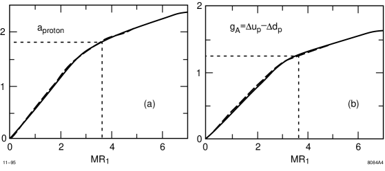
Figure 3: (a). The anomalous magnetic moment of the proton $a_{p}=F_{2}(0)$ as a function of its Dirac radius $M_{p}R_{1}$ in Compton units. (b). The axial vector coupling of the neutron to proton beta-decay as a function of $M_{p}R_{1}.$ In each figure, the broken line is computed from a wavefunction with power-law fall off and the solid curve is computed from a Gaussian wavefunction. The experimental values at the physical proton Dirac radius are indicated by the dotted line [82].

To obtain the ultra-relativistic limit we let $\beta\rightarrow\infty$ while keeping $m$ fixed. In this limit the proton becomes pointlike, $M_{p}R_{1}\rightarrow 0$, and the internal transverse momenta $k_{\perp}\rightarrow\infty$. The anomalous magnetic momentum of the proton goes linearly to zero as $a=0.43M_{p}R_{1}$ since $\langle\gamma_{V}\rangle\rightarrow 0$. Indeed, the Drell-Hearn-Gerasimov sum rule [83, 84] demands that the proton magnetic moment become equal to the Dirac moment at small radius. For a spin-$\frac{1}{2}$ system

$$a^{2}=\frac{M^{2}}{2\pi^{2}\alpha}\int_{s_{th}}^{\infty}\frac{ds}{s}\left[\sigma_{P}(s)-\sigma_{A}(s)\right]\;,$$ (40)

where $\sigma_{P(A)}$ is the total photoabsorption cross section with parallel (anti-parallel) photon and target spins. If we take the point-like limit, such that the threshold for inelastic excitation becomes infinite while the mass of the system is kept finite, the integral over the photoabsorption cross section vanishes and $a=0$. [15] In contrast, the anomalous magnetic moment of the proton does not vanish in the nonrelativistic quark model as $R\rightarrow 0$. The nonrelativistic quark model does not reflect the fact that the magnetic moment of a baryon is derived from lepton scattering at nonzero momentum transfer, i.e., the calculation of a magnetic moment requires knowledge of the boosted wavefunction. The Melosh transformation is also essential for deriving the DHG sum rule and low-energy theorems of composite systems [81].

A similar analysis can be performed for the axial-vector coupling measured in neutron decay. The coupling $g_{A}$ is given by the spin-conserving axial current $J_{A}^{+}$ matrix element

$$g_{A}(0)=\langle p,\uparrow|J^{+}_{A}|p,\uparrow\rangle\;.$$ (41)

The value for $g_{A}$ can be written as $g_{A}=\langle\gamma_{A}\rangle g_{A}^{\rm NR}$, with $g_{A}^{\rm NR}$ being the nonrelativistic value of $g_{A}$ and with $\gamma_{A}$ given by [92, 93]

$$\gamma_{A}(x_{i},k_{\perp i},m)=\frac{(m+x_{3}{\cal M})^{2}-k_{\perp 3}^{2}}{(m+x_{3}{\cal M})^{2}+k_{\perp 3}^{2}}\;.$$ (42)

In Fig. 3(b) the axial-vector coupling is plotted against the proton radius $M_{p}R_{1}$. The same parameters and the same line representation as in Fig. 3(a) are used. The functional dependence of $g_{A}(M_{p}R_{1})$ is also found to be independent of the assumed wavefunction. At the physical proton radius $M_{p}R_{1}=3.63$, one predicts the value $g_{A}=1.25$ (indicated by the dotted lines in Fig. 3(b)), since $\langle\gamma_{A}\rangle=0.75$. The measured value is $g_{A}=1.2573\pm 0.0028$ [94]. This is a 25% reduction compared to the nonrelativistic SU(6) value $g_{A}=5/3,$ which is only valid for a proton with large radius $R_{1}\gg 1/M_{p}.$ The Melosh rotation generated by the internal transverse momentum [93] spoils the usual identification of the $\gamma^{+}\gamma_{5}$ quark current matrix element with the total rest-frame spin projection $s_{z}$, thus resulting in a reduction of $g_{A}$.

Thus, given the empirical values for the proton’s anomalous moment $a_{p}$ and radius $M_{p}R_{1},$ its axial-vector coupling is automatically fixed at the value $g_{A}=1.25.$ This is an essentially model-independent prediction of the three-quark structure of the proton in QCD. The Melosh rotation of the light-cone wavefunction is crucial for reducing the value of the axial coupling from its nonrelativistic value 5/3 to its empirical value. The near equality of the ratios $g_{A}/g_{A}(R_{1}\rightarrow\infty)$ and $a_{p}/a_{p}(R_{1}\rightarrow\infty)$ as a function of the proton radius $R_{1}$ shows the wave-function independence of these quantities. We emphasize that at small proton radius the light-cone model predicts not only a vanishing anomalous moment but also $\lim_{R_{1}\rightarrow 0}g_{A}(M_{p}R_{1})=0$. One can understand this physically: in the zero radius limit the internal transverse momenta become infinite and the quark helicities become completely disoriented. This is in contradiction with chiral models, which suggest that for a zero radius composite baryon one should obtain the chiral symmetry result $g_{A}=1$.

The helicity measures $\Delta u$ and $\Delta d$ of the nucleon each experience the same reduction as does $g_{A}$ due to the Melosh effect. Indeed, the quantity $\Delta q$ is defined by the axial current matrix element

$$\Delta q=\langle p,\uparrow|\overline{q}\gamma^{+}\gamma_{5}q|p,\uparrow\rangle\;,$$ (43)

and the value for $\Delta q$ can be written analytically as $\Delta q=\langle\gamma_{A}\rangle\Delta q^{\rm NR}$, with $\Delta q^{\rm NR}$ being the nonrelativistic or naive value of $\Delta q$ and $\gamma_{A}$ given by Eq. (42).

The light-cone model also predicts that the quark helicity sum $\Delta\Sigma=\Delta u+\Delta d$ vanishes as a function of the proton radius $R_{1}$. Since $\Delta\Sigma$ depends on the proton size, it cannot be identified as the vector sum of the rest-frame constituent spins. The rest-frame spin sum is not a Lorentz invariant for a composite system [93]. Empirically, one can measure $\Delta q$ from the first moment of the leading-twist polarized structure function $g_{1}(x,Q).$ In the light-cone and parton model descriptions, $\Delta q=\int_{0}^{1}dx[q^{\uparrow}(x)-q^{\downarrow}(x)]$, where $q^{\uparrow}(x)$ and $q^{\downarrow}(x)$ can be interpreted as the probability for finding a quark or antiquark with longitudinal momentum fraction $x$ and polarization parallel or anti-parallel to the proton helicity in the proton’s infinite momentum frame [16]. [In the infinite momentum frame there is no distinction between the quark helicity and its spin projection $s_{z}.$] Thus $\Delta q$ refers to the difference of helicities at fixed light-cone time or at infinite momentum; it cannot be identified with $q(s_{z}=+\frac{1}{2})-q(s_{z}=-\frac{1}{2}),$ the spin carried by each quark flavor in the proton rest frame in the equal-time formalism.

Thus the usual SU(6) values $\Delta u^{\rm NR}=4/3$ and $\Delta d^{\rm NR}=-1/3$ are only valid predictions for the proton at large $MR_{1}.$ At the physical radius the quark helicities are reduced by the same ratio 0.75 as is $g_{A}/g_{A}^{\rm NR}$ due to the Melosh rotation. Qualitative arguments for such a reduction have been given elsewhere [95, 96]. For $M_{p}R_{1}=3.63,$ the three-quark model predicts $\Delta u=1,$ $\Delta d=-1/4,$ and $\Delta\Sigma=\Delta u+\Delta d=0.75$. Although the gluon contribution $\Delta G=0$ in our model, the general sum rule [97]

$$\frac{1}{2}\Delta\Sigma+\Delta G+L_{z}=\frac{1}{2}$$ (44)

is still satisfied, since the Melosh transformation effectively contributes to $L_{z}$.

Suppose one adds polarized gluons to the three-quark light-cone model. Then the flavor-singlet quark-loop radiative corrections to the gluon propagator will give an anomalous contribution $\delta(\Delta q)=-\frac{\alpha_{s}}{2\pi}\Delta G$ to each light quark helicity [98]. The predicted value of $g_{A}=\Delta u-\Delta d$ is of course unchanged. For illustration we shall choose $\frac{\alpha_{s}}{2\pi}\Delta G=0.15$. The gluon-enhanced quark model then gives the values in Table 1, which agree well with the present experimental values. Note that the gluon anomaly contribution to $\Delta s$ has probably been overestimated here due to the large strange quark mass. One could also envision other sources for this shift of $\Delta q$ such as intrinsic flavor [96]. A specific model for the gluon helicity distribution in the nucleon bound state is given elsewhere [18].

Quantity	NR	$3q$	$3q+g$	Experiment
$\Delta u$	$\frac{4}{3}$	1	0.85	$0.83\pm 0.03$
$\Delta d$	$-\frac{1}{3}$	$-\frac{1}{4}$	–0.40	$-0.43\pm 0.03$
$\Delta s$	0	0	–0.15	$-0.10\pm 0.03$
$\Delta\Sigma$	1	$\frac{3}{4}$	0.30	$0.31\pm 0.07$

Table 1: Comparison of the quark content of the proton in the nonrelativistic quark model (NR), in the three-quark model ($3q$), in a gluon-enhanced three-quark model ($3q+g$), and with experiment [99].

In the above analysis of the singlet moments, it is assumed that all contributions to the sea quark moments derive from the gluon anomaly contribution $\delta(\Delta q)=-\frac{\alpha_{s}}{2\pi}\Delta G$. In this case the strange and anti-strange quark distributions will be identical. On the other hand, if the strange quarks derive from the intrinsic structure of the proton, then one would not expect this symmetry. For example, in the intrinsic strangeness wavefunctions, the dominant fluctuations in the nucleon wavefunction are most likely dual to intermediate $\Lambda$-$K$ configurations since they have the lowest off-shell light-cone energy and invariant mass. In this case $s(x)$ and $\overline{s}(x)$ will be different.

The light-cone formalism also has interesting consequences for spin correlations in jet fragmentation. In LEP or SLC one produces $s$ and $\overline{s}$ quarks with opposite helicity. This produces a correlation of the spins of the $\Lambda$ and $\overline{\Lambda}$, each produced with large $z$ in the fragmentation of their respective jet. The $\Lambda$ spin essentially follows the spin of the strange quark since the $ud$ has $J=0$. However, this cannot be a 100% correlation since the $\Lambda$ generally is produced with some transverse momentum relative to the $s$ jet. In fact, from the light-cone analysis of the proton spin, we would expect no more than a 75% correlation since the $\Lambda$ and proton radius should be almost the same. On the other hand if $z=E_{\Lambda}/E_{s}\to 1,$ there can be no wasted energy in transverse momentum. At this point one could have 100% polarization. In fact, the nonvalence Fock states will be suppressed at the extreme kinematics, so there is even more reason to expect complete helicity correlation in the endpoint region.

We can also apply a similar idea to the study of the fragmentation of strange quarks to $\Lambda$s produced in deep inelastic lepton scattering on a proton. One can use the correlation between the spin of the target proton and the spin of the $\Lambda$ to directly measure the strange polarization $\Delta s.$ It is conceivable that any differences between $\Delta s$ and $\Delta\overline{s}$ in the nucleon wavefunction could be distinguished by measuring the correlations between the target polarization and the $\Lambda$ and $\overline{\Lambda}$ polarization in deep inelastic lepton proton collisions or in the target polarization region in hadron-proton collisions.

In summary, we have shown that relativistic effects are crucial for understanding the spin structure of nucleons. By plotting dimensionless observables against dimensionless observables, we obtain relations that are independent of the momentum-space form of the three-quark light-cone wavefunctions. For example, the value of $g_{A}\simeq 1.25$ is correctly predicted from the empirical value of the proton’s anomalous moment. For the physical proton radius $M_{p}R_{1}=3.63$, the inclusion of the Wigner-Melosh rotation due to the finite relative transverse momenta of the three quarks results in a $\sim 25\%$ reduction of the nonrelativistic predictions for the anomalous magnetic moment, the axial vector coupling, and the quark helicity content of the proton. At zero radius, the quark helicities become completely disoriented because of the large internal momenta, resulting in the vanishing of $g_{A}$ and the total quark helicity $\Delta\Sigma.$

10 CONCLUSIONS

One of the central problems in particle physics is to determine the structure of hadrons in terms of their fundamental QCD quark and gluon degrees of freedom. As I have outlined in this talk, the light-cone Fock representation of quantum chromodynamics provides both a tool and a language for representing hadrons as fluctuating composites of fundamental quark and gluon degrees of freedom. Light-cone quantization provides an attractive method to compute this structure from first principles in QCD. However, much more progress in theory and in experiment will be needed to fulfill this promise.

Acknowledgements

Much of this talk is based on an earlier review written in collaboration with Dave Robertson and on collaborations with Matthias Burkardt, Sid Drell, John Hiller, Kent Hornbostel, Paul Hoyer, Hung Jung Lu, Bo-Qiang Ma. Al Mueller, Chris Pauli, Steve Pinsky, Felix Schlumpf, Ivan Schmidt, Wai-Keung Tang, and Ramona Vogt. I also thank Simon Dalley and Francesco Antonuccio for helpful discussions.

References

- [1] P. A. M. Dirac, Rev. Mod. Phys. 21, 392 (1949); S. Weinberg, Phys. Rev. 150, 1313 (1966).
- [2] S. J. Brodsky and H.-C. Pauli, in Recent Aspects of Quantum Fields, H. Mitter and H. Gausterer, Eds., Lecture Notes in Physics, Vol. 396 (Springer-Verlag, 1991), and references therein.
- [3] M. Burkardt, Nucl. Phys. A 504, 762 (1989).
- [4] K. Hornbostel, S. J. Brodsky, and H.-C. Pauli, Phys. Rev. D 41, 3814 (1990).
- [5] K. Demeterfi, I. R. Klebanov, and G. Bhanot, Nucl. Phys. B 418, 15 (1994).
- [6] M. Krautgärtner, H.-C. Pauli, and F. Wölz, Phys. Rev. D 45, 3755 (1992); M. Kaluza and H.-C. Pauli, Phys. Rev. D 45, 2968 (1992).
- [7] J. R. Hiller, S. J. Brodsky, and Y. Okamoto, in progress (1995); J. R. Hiller, in Theory of Hadrons and Light-Front QCD, edited by St. D. Glazek (World Scientific, 1995), and talk presented at the 5th Meeting on Light-Cone Quantization and Nonperturbative QCD, Regensburg, Germany, June 1995.
- [8] M. Burkardt, Phys. Rev. D 49, 5446 (1994).
- [9] L.C.L. Hollenberg and N. S. Witte, Phys. Rev. D 50, 3382 (1994).
- [10] R. J. Perry, A. Harindranath and K. G. Wilson, Phys. Rev. Lett. 65, 2959 (1990).
- [11] R. J. Perry, Ann. Phys. 232, 116 (1994).
- [12] K. G. Wilson, T. S. Walhout, A. Harindranath, W.-M. Zhang, R. J. Perry, and St. D. Glazek, Phys. Rev. D 49, 6720 (1994).
- [13] M. Brisudova, talk presented at the 5th Workshop on Light-Cone QCD, Telluride, CO, August 1995; M. Brisudova and R. J. Perry, manuscript in preparation (1995).
- [14] S. D. Drell and T. M. Yan, Phys. Rev. Lett. 24, 181 (1970).
- [15] S. J. Brodsky and S. D. Drell, Phys. Rev. D 22, 2236 (1980).
- [16] G. P. Lepage and S. J. Brodsky, Phys. Rev. D 22, 2157 (1980).
- [17] S. J. Brodsky, P. Hoyer, A. H. Mueller, W.-K. Tang, Nucl. Phys. B369, 519 (1992).
- [18] S. J. Brodsky, M. Burkardt, and I. A. Schmidt, Nucl. Phys. B 441, 197 (1994).
- [19] H.-C. Pauli and S. J. Brodsky, Phys. Rev. D 32, 1993, 2001 (1985).
- [20] H. Bergknoff, Nucl. Phys. B 122, 215 (1977); T. Eller, H.-C. Pauli, and S. J. Brodsky, Phys. Rev. D 35, 1493 (1987); Y. Mo and R. J. Perry, J. Comp. Phys. 108, 159 (1993); K. Harada, A. Okazaki, and M. Taniguchi, Phys. Rev. D 52, 2429 (1995) and KYUSHU–HET 28, hep-th/9509136.
- [21] G. McCartor, Z. Phys. C 52, 611 (1991); ibid. 64, 349 (1994).
- [22] A. Harindranath and J. P. Vary, Phys. Rev. D 36, 1064, 1141 (1987); ibid. 37, 3010 (1988).
- [23] S. Dalley and I. R. Klebanov, Phys. Rev. D 47, 2517 (1993); G. Bhanot, K. Demeterfi, and I. R. Klebanov, Phys. Rev. D 48, 4980 (1993);
- [24] F. Antonuccio and S. Dalley, OUTP–9518P, hep-lat/9505009, and OUTP–9524P, hep-ph/9506456.
- [25] M. Burkardt, Phys. Rev. D 47, 4628 (1993).
- [26] St. D. Glazek, A. Harindranath, S. Pinsky, J. Shigemitsu, and K. G. Wilson, Phys. Rev. D 47, 1599 (1993); P. M. Wort, Phys. Rev. D 47, 608 (1993).
- [27] S. J. Brodsky and D. G. Robertson, SLAC-PUB-95-7056, OSU-NT-95- 06.
- [28] G. ’t Hooft, Nucl. Phys. B 75, 461 (1974).
- [29] C. J. Hamer, Nucl. Phys. B 195, 503 (1982).
- [30] G. D. Date, Y. Frishman and J. Sonnenschein, Nucl. Phys. B 283, 365 (1987).
- [31] M. Burkardt, New Mexico State University Preprint (1996), hep-ph/9601289.
- [32] S. J. Brodsky and G. R. Farrar, Phys. Rev. D 11, 1309 (1975).
- [33] G. Bertsch, S. J. Brodsky, A. S. Goldhaber, and J.F. Gunion, Phys. Rev. Lett. 47, 297 (1981).
- [34] S. J. Brodsky and A. H. Mueller, Phys. Lett. B 206, 685 (1988).
- [35] S. J. Brodsky and G. P. Lepage, in Perturbative Quantum Chromodynamics, edited by A. Mueller (World Scientific, Singapore, 1989).
- [36] S. J. Brodsky, G. P. Lepage, and P. Mackenzie, Phys. Rev. D28, 228 (1983).
- [37] S. J. Brodsky and H. J. Lu, Phys. Rev. D 51, 3652 (1995).
- [38] C. T. H. Davies, K. Hornbostel, G. P. Lepage, A. Lidsey, J. Shigemitsu, and J. Sloan, Phys. Lett. B 345, 42 (1995).
- [39] S. J. Brodsky, A. H. Hoang, J. H. Kühn, and T. Teubner, Phys. Lett. B 359, 355 (1995).
- [40] S. J. Brodsky, C. R. Ji, H. J. Lu, and A. Pang (in preparation).
- [41] S. J. Brodsky, L. Frankfurt, J. F. Gunion, A. H. Mueller, and M. Strikman, Phys. Rev. D 50, 3134 (1994).
- [42] Adams, et al., Phys. Rev. Lett. 74, 1525 (1995).
- [43] S. Heppelmann, Nucl. Phys. B (Proc. Suppl.) 12, 159 (1990), and references therein.
- [44] B. Blaettel, G. Baym, L.L. Frankfurt, H. Heiselberg, and M. Strikman, Phys. Rev. D 47, 2761 (1993).
- [45] S. J. Brodsky and B. T. Chertok, Phys. Rev. D 14, 3003 (1976).
- [46] S. J. Brodsky, C.-R. Ji, and G. P. Lepage, Phys. Rev. Lett. 51, 83 (1983).
- [47] G. R. Farrar, K. Huleihel, and H. Zhang, Phys. Rev. Lett. 74, 650 (1995).
- [48] A. D. Krisch, Nucl. Phys. B (Proc. Suppl.) 25, 285 (1992).
- [49] S. J. Brodsky and G. F. de Teramond, Phys. Rev. Lett. 60, 1924 (1988).
- [50] S. J. Brodsky, G. P. Lepage, and S. F. Tuan, Phys. Rev. Lett. 59, 621 (1987).
- [51] M. Luke, A. V. Manohar and M. J. Savage, Phys. Lett. B 288, 355 (1992).
- [52] S. J. Brodsky, G. F. de Teramond, and I. A. Schmidt, Phys. Rev. Lett. 64, 1011 (1990).
- [53] CDF Collaboration (F. Abe et al.), FERMILAB-PUB-95-271-E, Aug 1995.
- [54] E. Braaten and S. Fleming, Phys. Rev. Lett. 74, 3327 (1995).
- [55] G. T. Bodwin, E. Braaten, and G. P. Lepage, Phys. Rev. D 51, 1125 (1995).
- [56] S. J. Brodsky, P. Hoyer, C. Peterson, and N. Sakai, Phys. Lett. B 93, 451 (1980); S. J. Brodsky, C. Peterson, and N. Sakai, Phys. Rev. D 23 2745 (1981) .
- [57] S. J. Brodsky and Bo-Qiang Ma, SLAC-PUB 7126 (1996).
- [58] R. Vogt and S. J. Brodsky, Nucl. Phys. B 438, 261 (1995).
- [59] S. J. Brodsky, J. C. Collins, S. D. Ellis, J. F. Gunion, and A. H. Mueller, Snowmass Summer Study 1984:227 (QCD184:S7:1984).
- [60] J. J. Aubert, et al., Nucl. Phys. B 123, 1 (1983).
- [61] S. J. Brodsky, W.-K. Tang, and P. Hoyer, Phys. Rev. D52, 6285 (1995).
- [62] J. Badier, et al., Z. Phys. C 20, 1010 (1983).
- [63] C. Biino, et al., Phys. Rev. Lett. 58, 2523 (1987).
- [64] B. W. Harris, J. Smith, and R. Vogt, LBL-37266, (1995), hep-ph/9508403.
- [65] J. Badier, et al., Phys. Lett B 114, 457 (1982), ibid. 158, 85 (1985).
- [66] R. E. Ecclestone and D. M. Scott, Phys. Lett. B 120, 237 (1983).
- [67] V. G. Kartvelishvili and S. E’sakiya, Sov. J. Nucl. Phys. 38(3), 430 (1983) [Yad. Fiz. 38, 772 (1983)].
- [68] B. A. Li and K. F. Liu, Phys. Rev. D 29, 426 (1984).
- [69] V. Barger, F. Halzen, and W. Y. Keung, Phys. Lett. B 119, 453 (1983).
- [70] See J. D. Bjorken, J. B. Kogut, and D. E. Soper, Phys. Rev. D3, 1382 (1971), and references therein.
- [71] A summary of light-cone perturbative-theory calculation rules for gauge theories is given by Lepage and Brodsky [16]. We follow the notation of this reference here.
- [72] This is the light-cone analog of the infinite-momentum frame introduced in S. D. Drell. D. J. Levy, and T. M. Yan, Phys. Rev. Lett. 22, 744 (1969). See also S. J. Brodsky, F. E. Close, and J. F. Gunion, Phys. Rev. D6, 177 (1972).
- [73] The polarization of each vector-boson constituent is specified by the helicity index in as in Eq. (22).
- [74] We use momentum conservation to eliminate the dependence of on , where is the struck quark. Note that the results (15), (16), and (20) are independent of the charge of the constituents.
- [75] Related calculations in the infinite-momentum frame are given in S. J. Chang and S. K. Ma, Phys. Rev. 180, 1506 (1969); Bjorken, et al., Ref. [70]; D. Foerster, Ph.D. Thesis, University of Sussex, 1972; and S. J. Brodsky, R. Roskies, and R. Suaya, Phys. Rev. D8, 4574 (1973). The infinite-momentum-frame calculation of the order- contribution to the anomalous moment of the electron is also given in the last reference.
- [76] S. J. Brodsky, T. Huang, and G. P. Lepage, SLAC-PUB-2540 (unpublished).
- [77] Parton-model expression for other definitions of the charge radius are given in F. E. Close, F. Halzen, and D. M. Scott, Phys. Lett. 68B, 447 (1977).
- [78] For example, the contribution to the nucleon anomalous moment in the quark model gives a contribution if there is a trilinear coupling of scalars. It is thus possible to obtain a contribution to the anomalous moment of a fermion which is linear in its mass even if all of its consituent fermions are massless.
- [79] A better estimate is , where .
- [80] S. J. Brodsky and J. R. Hiller, Phys. Rev. C 28, 475 (1983).
- [81] S. J. Brodsky and J. R. Primack, Ann. Phys. 52 315 (1969); Phys. Rev. 174, 2071 (1968).
- [82] S. J. Brodsky and F. Schlumpf, Phys. Lett. B 329, 111 (1994).
- [83] S. B. Gerasimov, Yad. Fiz. 2, 598 (1965) [Sov. J. Nucl. Phys. 2, 430 (1966)].
- [84] S. D. Drell and A. C. Hearn, Phys. Rev. Lett. 16, 908 (1966).
- [85] B.-Q. Ma, Phys. Rev. C 43 2821 (1991); Int. J. Mod. Phys. E 1 809 (1992) .
- [86] F. Schlumpf, Phys. Rev. D 47, 4114 (1993); Mod. Phys. Lett. A 8, 2135 (1993); Phys. Rev. D 48, 4478 (1993); J. Phys. G 20, 237 (1994).
- [87] E. Wigner, Ann. Math. 40, 149 (1939).
- [88] H. J. Melosh, Phys. Rev. D 9, 1095 (1974); L. A. Kondratyuk and M. V. Terent’ev, Yad. Fiz. 31, 1087 (1980) [Sov. J. Nucl. Phys. 31, 561 (1980)]; D. V. Ahluwalia and M. Sawicki, Phys. Rev. D 47, 5161 (1993).
- [89] L. L. Frankfurt and M. I. Strikman, Nucl. Phys. B 148, 107 (1979), Phys. Rep. 76, 215 (1981); L. A. Kondratyuk and M. I. Strikman, Nucl. Phys. A 426, 575 (1984); L. L. Frankfurt, T. Frederico, and M. Strikman, Phys. Rev. C 48, 2182 (1993).
- [90] F. Coester and W. N. Polyzou, Phys. Rev. D 26, 1349 (1982); P. L. Chung, F. Coester, B. D. Keister and W. N. Polyzou, Phys. Rev. C 37, 2000 (1988).
- [91] H. Leutwyler and J. Stern, Ann. Phys. 112, 94 (1978).
- [92] P. L. Chung and F. Coester, Phys. Rev. D 44, 229 (1991).
- [93] B.-Q. Ma, J. Phys. G. 17, L53 (1991); B.-Q. Ma and Qi-Ren Zhang, Z. Phys. C 58, 479 (1993).
- [94] Particle Data Group, Phys. Rev. D 45 (Part 2), 1 (1992).
- [95] G. Karl, Phys. Rev. D 45, 247 (1992).
- [96] H. Fritzsch, Mod. Phys. Lett. A 5, 625 (1990).
- [97] R. L. Jaffe and A. Manohar, Nucl. Phys. B 337, 509 (1990).
- [98] A. V. Efremov and O. V. Teryaev, Proceedings of the International Symposium on Hadron Interactions (Bechyne), eds. J. Fischer, P. Kolar and V. Kundrat (Prague), 302 (1988); G. Altarelli and G. G. Ross, Phys. Lett. B 212, 391 (1988); R. D. Carlitz, J. C. Collins and A. H. Mueller, Phys. Lett. B 214, 229 (1988).
- [99] J. Ellis and M. Karliner, Phys. Lett. B 341, 397 (1995).