20 April 1996 CBPF-NF-020/96      hep - ph

QCD EVOLUTION OF THE GLUON
DENSITY IN A NUCLEUS
A. L. Ayala F${}^{\underline{o}}$ ${}^{a)\,b)}$^∗ , M. B. Gay Ducati ^a)∗∗
and

E.M. Levin ${}^{\dagger}\,{}^{c)\,d)}$

^a)Instituto de Física, Univ. Federal do Rio Grande do Sul
Caixa Postal 15051, 91501-970 Porto Alegre, RS, BRAZIL
^b)Instituto de Física e Matemática, Univ. Federal de Pelotas
Campus Universitario, Caixa Postal 354, 96010-900, Pelotas, RS, BRAZIL
^c) LAFEX, Centro Brasileiro de Pesquisas Físicas (CNPq)
Rua Dr. Xavier Sigaud 150, 22290 - 180 Rio de Janeiro, RJ, BRAZIL

^d) Theory Department, Petersburg Nuclear Physics Institute
188350, Gatchina, St. Petersburg, RUSSIA

Abstract: The Glauber approach to the gluon density in a nucleus, suggested by A. Mueller, is developed and studied in detail. Using the GRV parameterization for the gluon density in a nucleon, the value as well as energy and $Q^{2}$ dependence of the gluon density in a nucleus is calculated. It is shown that the shadowing corrections are under theoretical control and are essential in the region of small $x$. They change crucially the value of the gluon density as well as the value of the anomalous dimension of the nuclear structure function, unlike of the nucleon one. The systematic theoretical way to treat the correction to the Glauber approach is developed and a new evolution equation is derived and solved. It is shown that the solution of the new evolution equation can provide a selfconsistent matching of “soft” high energy phenomenology with “hard” QCD physics.

1 Introduction.

In this paper we discuss the QCD evolution for the gluon density in a nucleus. The gluon density is the most important physical observable that governs the physics at high energy (low Bjorken $x$) in deep inelastic processes [1]. Dealing with nucleus we have to take into account the shadowing correction (SC) due to rescattering of the gluon inside the nucleus, which is the main point of interest in this paper. We show that SC can be treated theoretically in the framework of perturbative QCD (pQCD) and can be calculated using the information on the behavior of the gluon structure function for the nucleon.

Our calculations were performed in the double log approximation ( DLA) of pQCD, or in other words in the GLAP evolution equations [2] for the region of low $x$ ( high energy ). In the DLA we consider the kinematic region where $\alpha_{\rm S}\ln(1/x)\,\ln(Q^{2}/Q^{2}_{0})\,\,\sim\,\,1$ while $\alpha_{\rm S}\ln(1/x)\,\,\ll\,\,1$ and $\alpha_{\rm S}\ln(Q^{2}/Q^{2}_{0})\,\,\ll\,\,1$ as well as $\alpha_{\rm S}\,\,\ll\,\,1$, where $Q^{2}$ is the virtuality of the photon and $\alpha_{\rm S}$ is the QCD coupling constant. In terms of the anomalous dimension ( see the next section for details) it means that we restrict ourselves by considering only the leading term in the anomalous dimension, namely $\gamma$ being $\alpha_{\rm S}\,\ll\,\gamma\,\ll\,1$.

The advantages of the DLA are (see Fig.1 for notations):

1) we can neglect the change in the distance between quark (gluon) and antiquark (gluon) $r_{t}$ during the passage of the $q\bar{q}$ ( GG) pair through the nucleus. This simplifies the derivation of all formulae for the SC and leads to an eikonal picture of classical propagation of the $q\bar{q}$ (GG) pair with high energy which receives independent kicks due to rescattering in a nucleus.

2) the cross section of the $q\bar{q}$ (GG) pair with transverse separation $r_{t}$ can be expressed through the gluon deep inelastic structure function for a nucleon.

Figure 1: The structure of the parton cascade in the Glauber formula. $A$ denotes the nucleus, N - the nucleon, $G^{*}(Q^{2})$ - the virtual gluon and $\sigma_{N}(r^{2}_{t})$ is the nucleon cross section.

We will discuss both points in the next section in more detail. However, it is worthwhile mentioning that the DLA allows us to obtain the simplest and closest expression for the SC in DIS with a nucleus.

The main goal of the paper is (i) to present a study of the SC in the Glauber approach using available information on the gluon distribution in the nucleon based mainly on new experimental data from HERA [3] and on the solution of the GLAP evolution equations [2]; and (ii) to find the generalization of the Glauber approach which will give the theoretical basis for the selfconsistent description of the gluon structure function for nuclei.

Considering the deep inelastic scattering (DIS), we have to answer two principal questions: (i) why and how the cross section of DIS with nucleus which is equal to $\sigma(\gamma^{*}A)\,=\,A\,\sigma(\gamma^{*}p)$ at $x\,\approx\,1$ changes its A-dependence and becomes $\sigma(\gamma^{*}A)\,\propto\,A^{\frac{2}{3}}$ at $x\,\rightarrow\,0$ ; and (ii) why $\sigma(\gamma^{*}A)$, which is proportional to $A^{\frac{2}{3}}$ at small values of $x$ and $Q^{2}$, approaches to $\sigma(\gamma^{*}A)=A\sigma(\gamma^{*}p)$ at large values of $Q^{2}$ even in the region of small $x$. The last statement is obvious from the intuitive physical picture because at large values of $Q^{2}$ $\sigma(\gamma^{*}p)$ is small and the virtual photon probes the number of nucleons in a nucleus.

The first question has been answered in the framework of the parton model ( see refs.[4] [5][6]) and the answer is based on the space-time picture of DIS in the rest frame of the nucleus. Indeed, the incident electron penetrates the nucleus and radiates the virtual photon whose lifetime $\tau_{\gamma^{*}}\,\propto\,\frac{1}{mx}$ [4]. We can recover three different kinematic regions:

1. $\tau_{\gamma^{*}}\,=\,\frac{1}{mx}\,\,<\,\,R_{NN}$, where $R_{NN}$ is the characteristic distances between the nucleons of the nucleus. This virtual photon can be absorbed only by one nucleon and the total cross section is $\sigma(\gamma^{*}A)\,=\,A\,\sigma(\gamma^{*}p)$.

2. $R_{A}\,\,>\,\,\tau_{\gamma^{*}}\,=\,\frac{1}{mx}\,\,>\,\,R_{NN}$, where $R_{A}$ is the nucleus radius. In this kinematic region the virtual photon can interact with the group of nucleons. However, $\sigma(\gamma^{*}A)$ is still proportional to $A$ since the number of nucleons in a group is much less than $A$.

3. $\tau_{\gamma^{*}}\,=\,\frac{1}{mx}\,\,>\,\,R_{A}$. Here, before reaching the front surface of the nucleus, the virtual photon “decomposes” in the developed parton cascade which then interacts with the nucleus. It can be shown [5] that the absorption cross section of the virtual photon will now be proportional to the surface area of the nucleus $\sigma(\gamma^{*}A)\,\propto\,A^{\frac{2}{3}}$, because the wee partons of the parton cascade are absorbed at the surface and do not penetrate into the centre of the nucleus.

However, the above simple picture cannot help us to answer the second question. Indeed, we can use it to explain the $A$ dependence of the initial partonic distributions but in the GLAP evolution equations the $A$ dependence is factorized out and do not affect the $Q^{2}$ evolution. Therefore, we have to change the evolution equations to incorporate the physical phenomenon which we have formulated as the second question. To recover the physical origin of the new evolution equations in nucleus let us consider the oversimplified structure of the parton cascade: the virtual photon decays only in quark - antiquark pair. In this case the cross section can be written in the form:

$$\sigma(\gamma^{*},A)\,\,\propto\,\,\int^{1}_{0}dz\int d^{2}r_{t}\Psi(z,r_{t})\,\sigma_{A}(zQ_{0},r^{2}_{t})\,\Psi^{*}(z,r_{t})$$ (1)

where $\sigma_{A}$ is the cross section for $\bar{q}q$ interaction with the nucleus, $z$ is the fraction of energy of the photon ($Q_{0}$) carried by quark and $r_{t}$ is the transverse separation between quark and antiquark. $\Psi$ is the wave function of the virtual photon, which is known and $|\Psi|^{2}$ is equal to $a^{2}K^{2}_{1}(ar_{t})[z^{2}+(1-z)^{2}]$, where $K_{1}$ is the McDonald function and $a^{2}=Q^{2}z(1-z)$. The main contribution in the eq. (1) comes from the region where $ar_{t}\,<\,1$. Expanding $K_{1}$ and integrating over $z(1-z)\,<\frac{1}{Q^{2}r^{2}_{t}}\,<\,\frac{1}{4}$ we derive

$$\sigma(\gamma^{*},A)\,\,\propto\,\,\frac{1}{Q^{2}}\int^{\infty}_{\frac{4}{Q^{2}}}\frac{dr^{2}_{t}}{r^{4}_{t}}\,\sigma_{A}(\frac{Q_{0}}{Q^{2}r^{2}_{t}},r^{2}_{t})\,$$ (2)

For very small $r_{t}$ the cross section in QCD is small and proportional to $r^{2}_{t}$. Such small cross section leads to $\sigma_{A}\,\propto\,A\,\frac{1}{Q^{2}}\ln Q^{2}$, since the probe with small cross section interacts with all nucleons in the nucleus. One can see that this is the first term of the GLAP evolution equations. With more complicated parton cascade we are able to reconstruct the GLAP evolution equations in a full. However, even at small $r^{2}_{t}$, $\sigma_{A}=A\sigma_{N}$ only if the rescattering of $\bar{q}q$ - pair in a nucleus is small. The parameter which controls the value of the rescatterings is the number of collisions which is equal $\nu\,=\,2\,\sigma_{N}\,\rho\,R_{A}$, where $\rho$ is the nucleon density in the nucleus. If $\nu\,\ll\,1$ we can neglect the rescatterings,but if $\nu\,\gg\,1$ $\sigma_{A}\,=\,2\pi R^{2}_{A}$ and does not depend on nucleon cross section. Therefore, we can trust the $\ln Q^{2}$ contribution in eq. (2) only for $\nu=r^{2}_{t}\rho R_{A}\,<\,1$ or for $Q^{2}>\rho R_{A}$. Really, this condition depends on $x$ too, since the nucleon cross section is a function of $x$, namely we will show that $\sigma_{N}\,\propto\,r^{2}_{t}xG(x,\frac{1}{r^{2}_{t}})$.

Therefore, the lesson learned from this simple exercise is that we can trust the GLAP evolution for the nucleus structure function only for $Q^{2}\,>\,Q^{2}_{0}(x)$. It means that we have to solve the GLAP evolution equation with the initial condition on the line $Q^{2}=Q^{2}_{0}(x)$ or we have to change the evolution equations if we want to solve them in an usual way, namely, starting from the structure functions at $Q^{2}=Q^{2}_{0}$.

The previous attempts to attack this problem were related to the GLR equation [1, 7], in which the interaction ( recombination ) between two partons from different parton cascades was taken into account ( see refs.[8, 7, 9, 10, 11, 12] ). It was shown that the GLR equation is able to describe the main features of the experimental data on the deep inelastic scattering off nucleus [14, 13]. The applications of the same ideas to description of other process such as J/$\Psi$ production [15] and Drell-Yan process [16] was also with reasonable success [17, 18].

However, the GLR equation was derived in the limited kinematic region where more complicated recombination processes have been proven to be negligible. Roughly speaking, we can trust the GLR equation only for small $x$ and big values of $Q^{2}$.

In this paper we reanalyse the situation with the shadowing corrections in QCD for nucleus gluon structure function starting with the Glauber approach. The Glauber formula for the gluon structure function in the nucleus has been proven by A. Mueller in ref.[19] but this was remained unnoticed by the majority of experts because his paper was devoted to quite different problem. In section 2 we rederive the Mueller formula and discuss the main properties of the Glauber approach in QCD.

In section 3, we present the result of our calculations based on Glauber approach and point out which information on nuclear gluon distribution is needed in order to provide a reliable calculation. We adopt to following semiquantative way to study the mechanism and value of the SC: we used the GRV parameterization for the gluon structure function in the nucleon, which describes quite well the current experimental data. However, we would like rather to study the main properties of the SC than to provide reliable predictions for an experiment.

In section 4 we consider the correction to the Glauber formula and discuss the generalization of the Glauber approach for deep inelastic scattering off nucleus. Here, we discuss the GLR evolution equation which was the basis of all previous attempts to go beyond the Glauber approach and suggest and solve a more general evolution equation which is correct in the whole kinematic region without the limitations of the GLR equation.

A summary and final discussion are presented is section 5.

2 The Glauber approach in QCD .

In this paper we will use the following notation (see Fig.1 and Fig.2):

$Q^{2}$ denotes the virtuality of the gluon in deep inelastic scattering (DIS);

$m$ is the mass of the proton nucleus specified otherwise;

Bjorken $x$ = $x_{Bj}\equiv\frac{Q^{2}}{s}$ where $\sqrt{s}\,=\,W$ is the c.m. energy of the incoming gluon.

$\vec{k}_{t}$ denotes the transverse momentum of the quark or gluon;

$\vec{r}_{t}$ is the transverse separation between quark (gluon) and antiquark (gluon);

$\vec{b}_{t}$ is the impact parameter of the reaction which is the variable conjugated to the momentum transfer ($\vec{q}_{t}$);

$\vec{l}_{1t}$ denotes the transverse momentum of the gluon attached to the quark - antiquark (gluon-gluon) pair.

Figure 2: Kinematics of diffractive production of a gluon pair. $Q^{*}$ is the virtual colorless probe of the gluon density.

We will use the GLAP evolution equations [2] for the parton densities in momentum space. For any function $f(x)$, we define the moment $f(\omega)$ as

$$f(\omega)=\int_{0}^{1}dx\,x^{\omega}f(x)\,.$$ (3)

Note that the moment variable $\omega$ is chosen such that the $\omega=0$ moment measure the number of partons, and the $\omega=1$ measure their momentum. An alternative moment variable $N=\omega-1$ is often found in the literature. The $x$-distribution can be reconstructed by considering the inverse Mellin transform. For example, for the gluon distribution it reads

$$xG(x,Q^{2})=\frac{1}{2\pi i}\int_{C}d\omega\,\,x^{-\omega}\,g(\omega,Q^{2})\,,\$$ (4)

where $g(\omega,Q^{2})$ is the moment of the gluon distribution. The contour of integration $C$ is taken to the right of all singularities.

The GLAP evolution equations have the solutions of the form

$$g(\omega,Q^{2})=g(\omega)e^{\gamma(\omega)lnQ^{2}}\,,$$ (5)

where $\gamma(\omega)$ denotes the anomalous dimension, which in the leading $ln(1/x_{B})$ approximation (LLA) of pQCD, is a function of $\alpha_{\rm S}/\omega$ and can be presented as the following series [20]:

$$\gamma(\omega)\,\,=\,\,\frac{\alpha_{\rm S}N_{c}}{\pi}\cdot\frac{1}{\omega}\,\,+\,\,\frac{2\alpha_{\rm S}^{4}N_{c}^{4}\zeta(3)}{\pi^{4}}\cdot\frac{1}{\omega^{4}}\,\,+\,\,O(\frac{\alpha_{\rm S}^{5}}{\omega^{5}})$$ (6)

where $\zeta(3)$ is the Riemman zeta function, and $N_{c}$ is the number of colors. In DLA, only the first term in the above series is taken into account.

The amplitude is normalized such that

$$\frac{d\sigma}{dt}\,\,=\,\,\pi\,|f(s,t)|^{2}\,\,,$$ (7)

$$\sigma_{tot}\,\,=\,\,4\pi\,\,Im\,f(s,0)\,\,,$$ (8)

and the scattering amplitude in $b_{t}$-space is defined as

$$a(s,b_{t})\,\,=\,\,\frac{1}{2\pi}\,\,\int\,\,d^{2}q_{t}\,\,e^{-i{\vec{q}}_{t}\,\cdot\,{\vec{b}}_{t}}\,\,f(s,t=-q^{2}_{t})\,.$$ (9)

In this representation

$$\sigma_{tot}\,\,=\,\,2\,\,\int\,d^{2}b_{t}\,\,Im\,\,a(s,b_{t}),$$ (10)

$$\sigma_{el}\,\,=\,\,\int\,d^{2}b_{t}\,\,|\,a(s,b_{t})|^{2}.$$ (11)

The normalization of the nucleus wave function $\Psi_{A}(r_{1},...r_{i},r_{A})$ is

$$\int\Psi_{A}(r_{1},...r_{i},r_{A})\Psi_{A}^{*}(r_{1},...r_{i},r_{A})\prod_{i=1}^{A}d^{3}r_{i}=A\,\,,$$ (12)

where $A$ is the number of nucleons in the nucleus, and the nucleon form factor in the nucleus is defined as

$$F_{A}(q_{z},b_{t})=\int\,d\,z_{1}\,e^{iq_{z}z_{1}}\Psi_{A}(z_{1},b_{t},r_{2},...r_{i},r_{A})\Psi_{A}^{*}(z_{1},b_{t},r_{2},...r_{i},r_{A})\prod_{i=2}^{A}d^{3}r_{i}\,.$$ (13)

Throughout this paper we use the Gaussian parameterization for $F_{A}(q_{z},b_{t})$, namely

$$F_{A}(q_{z},b_{t})=\frac{A}{\pi R_{A}^{2}}e^{-\frac{b_{t}^{2}}{R_{A}^{2}}-\frac{R_{A}^{2}}{4}q_{z}^{2}}\,,$$ (14)

where the mean radius of the nucleus $R_{A}^{2}$ is equal to

$$R_{A}^{2}=\frac{2}{5}R_{WS}^{2}\,\,,$$ (15)

and $R_{WS}^{2}$ is the size of the nucleus in the Wood-Saxon parameterization[21], which we choose $R_{WS}^{2}=r_{0}A^{1/3}$ with $r_{0}=1.3fm$.

In nonrelativistic theory for the nucleus we can neglect the change of energy for the recoil nucleon. Its energy is $E_{p^{\prime}}=m+q^{2}/2m$ in the rest frame of the nucleus and $q^{2}/2m\ll q_{z}$.

2.1 Passage of the $\bar{q}q$ ($GG$) pair through the target

The idea how to write the Glauber formula in QCD was originally formulated in Ref.[22] and it has been carefully developed in Ref.[19]. It is easier to explain the main idea considering the penetration of quark anti-quark pair, produced by the virtual photon, through the target. While the boson projectile is traversing the target, the distance $r_{t}$ between the quark and anti-quark can vary by amount $\Delta r_{t}\propto R_{A}\frac{k_{t}}{E}$ where $E$ denotes the energy of the pair in the target rest frame and $R_{A}$ is the size of the target (see Fig.2).

Figure 3: The structure of parton cascade in the Glauber ( Mueller ) formula.

The quark transverse momentum is $k_{t}\propto 1/r_{t}$. Therefore

$$\Delta\,r_{t}\,\propto\,R\,\,\frac{k_{t}}{E}\,\,\ll\,\,r_{t}\,,$$ (16)

and is valid if

$$\,r^{2}_{t}\,s\,\,\gg\,\,\,2\,m\,R\,,$$ (17)

where $s=2mE$. In terms of Bjorken $x$, the above condition looks as follows

$$x\,\,\ll\,\,\frac{1}{2\,m\,R}\,.$$ (18)

Therefore the transverse distance between quark and antiquark is a good degree of freedom [19][23][24]. As has been shown by A.Mueller, not only quark - antiquark pairs can be considered in such way. The propagation of a gluon through the target can be treated in a similar way as the interaction of gluon - gluon pair with definite transverse separation $r_{t}$ with the target. It is easy to understand if we remember that virtual colorless graviton or Higgs boson is a probe of the gluon density.

The total cross section of the absorption of gluon($G^{*}$) with virtuality $Q^{2}$ and Bjorken $x$ can be written in the form:

$$\sigma^{A}_{tot}(\,G^{*}\,)\,\,=\,\,$$ (19)

$$\int^{1}_{0}dz\,\,\int\,\frac{d^{2}r_{t}}{2\pi}\,\,\int\frac{d^{2}b_{t}}{2\pi}\Psi^{G^{*}}_{\perp}(Q^{2},r_{t},x,z)\,\,2\{1\,\,-\,\,exp[-\,\frac{1}{2}\sigma(r^{2}_{t})\,\,S(b^{2}_{t})\,]\,\}\,\,[{\Psi^{G^{*}}_{\perp}}(Q^{2},r_{t},x,z)]^{*}\,,$$

where $z$ is the fraction of energy which is carried by the gluon, $\Psi^{G^{*}}_{\perp}$ is the wave function of the transverse polarized gluon and $\sigma(r^{2}_{t})$ is the cross section of the interaction of the pair with transverse separation $r_{t}$ with the nucleon, and $S(b_{t})$ is the profile function of a nucleus which we will specify later.

The physical interpretation of Eq.$(17)$ is very simple, if one notices that the factor in curly brackets is the total cross section for the $GG$ pair with transverse separation $r_{t}$ passing through the nucleus

$$\sigma^{SC}_{tot}(r_{t})=2\int\frac{d^{2}b_{t}}{\pi}\{1\,\,-\,\,e^{-\,\frac{1}{2}\sigma_{N}(r^{2}_{t})\,\,S(b^{2}_{t})\,}\,\}\,.$$ (20)

Indeed, the above formula is a solution of the $s$-channel unitarity relation:

$$2\,\,Im\,a(s,b_{t})\,\,=\,\,|a(s,b_{t})|^{2}\,\,+\,\,G_{in}(s,b_{t})\,,$$ (21)

where $a$ denotes the elastic amplitude for the $GG$ pair with a transverse separation $r_{t}$, and $G_{in}$ is the contribution of all the inelastic processes. The inelastic cross section is equal to

$$\sigma_{in}\,\,=\,\,\int\,\,d^{2}\,b_{t}\,\,G_{in}(s,b_{t})\,\,=\,\,\int d^{2}b_{t}\,\,\left(\,\,1\,\,-\,\,e^{-\,\,\sigma_{N}(r_{t},q^{2}_{t}=0)\,\,S(b^{2}_{t})}\,\,\right)\,.$$ (22)

We assume that the form of the final state is a uniform parton distribution that follows from the QCD evolution equations. Note that we neglect the contribution of all diffraction dissociation processes to the inelastic final state (in particular to the “fan” diagrams which give an important contribution), as well as diffraction dissociation in the region of small masses, which cannot be presented as a decomposition of the $GG$ wave function. We evaluate this input hypothesis in section 4.

In the language of Feynman diagrams, Eq.(20) sums all diagrams of Fig.2 in which the $GG$ pair rescatters with the target, and exchanges “ladder” diagrams each of which corresponds to the gluon density. This sum has already been performed by Mueller[19], and we will only comment how one can obtain the result, without going into details. We borrow the presentation of the end of this subsection as well as the next two ones borrow Ref.[25].

The simplest way is to consider the inelastic cross section (see Refs.[19, 1, 26]), which has the direct interpretation through the parton wave function of the hadron (see Fig.3), as all partons that are produced are on the mass shell. In leading $ln{1}/{x}$ approximation we have two orderings in time:

1. The time of emission of each “ladder” by the fast $GG$ pair, which should obey the obvious ordering for $n$ produced “ladders” (see Fig.3)

$$t_{1}\,\,>\,\,t_{2}\,\,...\,\,>\,\,t_{i}\,\,>\,\,t_{i+1}\,\,...>\,\,t_{n}\,;$$ (23)

2. Each additional “ladder” which should live for a shorter time than the previous one. This gives a second ordering (see Fig.3):

$$t_{1}-t^{\prime}_{1}\,\,>\,\,t_{2}-t^{\prime}_{2}\,\,>\,\,...\,\,>\,\,t_{i}-t^{\prime}_{i}\,\,>\,\,...\,\,>\,\,t_{n}-t^{\prime}_{n}\,;$$ (24)

Each “ladder” in the leading log approximation is the same function of $t_{i}-t^{\prime}_{i}$ which we denote as $\sigma(t-t^{\prime},r^{2}_{t})$. This fact allows us to carry out the integration over $t_{i}$ and $t_{i}-t^{\prime}_{i}$, which gives for $n$ emitted cascades:

$$\sigma_{n}\,\,=\,\,\frac{1}{(n!)^{2}}\int^{t}dt_{1}\int^{t-t^{\prime}}d(t_{1}-t^{\prime}_{1})\,\,\sigma^{n}(t_{1}-t^{\prime}_{1},r^{2}_{t})\,.$$ (25)

For the case of the $GG$ pair, both last integrations are not logarithmic, and in the leading log approximation we can safely replace the above integral by

$$\sigma_{n}\,\,=\,\,\,\frac{1}{(n!)^{2}}\,\,\sigma^{n}(t-t^{\prime},r^{2}_{t})\,,$$ (26)

where $t-t^{\prime}$ is of the order of $\frac{1}{q_{\parallel}}$ due to uncertainty principle, where $q_{\parallel}\,\,=\,\,\frac{Q^{2}}{s}$. One $n!$ is compensated by the number of possible diagrams, since the order of the ”ladders” are not fixed. Therefore, the contribution of the $n$th “ladder” exchange gives

$$\sigma_{n}\,\,=\,\,\,\frac{1}{n!}\,\,\sigma^{n}(x,r^{2}_{t})\,.$$ (27)

Applying the AGK cutting rules[26] we reconstruct the total cross section which results in Eq.(20).

2.2 $\sigma(r_{t},q^{2}_{t})$ at $q_{t}$ = 0.

The expression for $\sigma(r_{t},q^{2}_{t})$ at $q_{t}=0.$ was first written down in Ref.[22] ( see Eq.(8) of this paper). It turns out that $\sigma$ can be expressed through the unintegrated parton function $\phi$ first introduced in the BFKL papers[27] and widely used in Ref.[1]. The relation of this function to the Feynman diagrams and the gluon density can be calculated using the following equation:

$$\alpha_{\rm S}(Q^{2})xG(x,Q^{2})\,\,=\,\,\int^{Q^{2}}\,\,dl^{2}_{t}\,\,\alpha_{\rm S}(l^{2}_{t})\,\,\phi(x,l^{2}_{t})$$ (28)

Using the above equation we reproduce the results of Ref.[22], which reads

$$\sigma(r_{t},q^{2}_{t})\,\,=\,\,\frac{16C_{F}}{N^{2}_{c}-1}\,\,\pi^{2}\int\phi(x,l^{2}_{t})\,\,\{\,\,1\,\,-\,\,e^{i\,\vec{l}_{t}\vec{r}_{t}}\,\,\}\,\,\frac{\alpha_{\rm S}(l^{2}_{t})}{2\pi}\,\frac{d^{2}l_{t}}{l^{2}_{t}}$$ (29)

where $\phi\,\,=\,\,\frac{\partial xG(x,Q^{2})}{\partial Q^{2}}$.

We evaluate this integral using Eqs.(4),(10) and (11) and integrate over the azimuthal angle. Introducing a new variable $\xi=r_{t}l_{t}$, the integral can be written in the form:

$$\sigma(r_{t},q^{2}_{t})\,\,=\,\,\frac{16C_{F}\alpha_{\rm S}}{N^{2}_{c}-1}\,\,\pi^{2}\int_{C}\frac{d\omega}{2\pi i}\,x^{-\omega}\,g(\omega)\,\,\gamma(\omega)\,\,(r^{2}_{t})^{1-\gamma(\omega)}\int^{\infty}_{0}d\,\,\xi\,\,\frac{1-J_{0}(\xi)}{(\xi)^{3-2\gamma(\omega)}}$$ (30)

Evaluating the integral over $\xi$ (see Ref.[34] 11.4.18) we have:

$$\sigma(r_{t},q^{2}_{t})\,\,=\,\,\frac{8C_{F}\alpha_{\rm S}}{N^{2}_{c}-1}\,\,\pi^{2}\int_{C}\frac{d\omega}{2\pi i}\,x^{-\omega}\,g(\omega)\,\,\gamma(\omega)\,\,(\frac{r^{2}_{t}}{4})^{1-\gamma(\omega)}\,\,\,\frac{\Gamma(\gamma(\omega))\,\,\Gamma(1-\gamma(\omega))}{(\,\Gamma(2-\gamma(\omega)\,))^{2}}$$ (31)

In the double log approximation of pQCD where $\gamma(\omega)\,\,\ll\,\,1$ the cross section for $N_{c}$ = 3 reads:

$$\sigma(r_{t},q^{2}_{t})\,\,=\,\,\frac{\alpha_{\rm S}(\frac{4}{r^{2}_{t}})}{3}\,\,\pi^{2}\,\,r^{2}_{t}\,\,\left(\,\,xG^{GLAP}(x,\frac{4}{r^{2}_{t}})\,\,\right)$$ (32)

This result coincides with the value of the cross section given in Refs.[28, 29] (if we neglect the factor 4 in the argument of the gluon density). We checked that Eq.(2.16) of Ref.[30] also leads to the same answer, unlike the value for $\sigma$ quoted in Ref.[16] (see Eq.(2.20)).

In the case of the passage of the $GG$ pair, Eq.(32) reads (for $N_{c}=3$)

$$\sigma(r_{t},q^{2}_{t}=0)=\frac{3\alpha_{\rm S}(\frac{4}{r^{2}_{t}})}{4}\pi^{2}r^{2}_{t}\left(xG_{N}^{GLAP}(x,\frac{4}{r^{2}_{t}})\right)$$ (33)

Eqs (32) and (33) are valid only on DLA of pQCD because we obtained these expressions considering $l_{it}\ll k_{t}$ and neglecting the longitudinal part of the momentum $l_{i}$ ($l_{i\parallel}\ll l_{it}$). It is very essential to realize this limitation of our approach for all further applications.

2.3 The $b_{t}$ dependence of the scattering amplitude with a nucleon

To deal with the SC we need to know the amplitude not only at $q_{t}=0$, but at all values of momentum transfer, so that we can calculate the profile function of the amplitude in impact parameter space. The gluon density in a nucleon depends only weakly on $q_{t}$ in the GLAP evolution (see Ref.[1] for details). Therefore, all the $q_{t}$-dependence comes from the form factor of the $G_{1}G_{2}$ ($\bar{q}q$) pair with the transverse separation $r_{t}$ and the form factor of the target nucleus.

The form factor for $G_{1}G_{2}$ ($\bar{q}q$) pair with the transverse separation $r_{t}$ is equal to

$$F_{G_{1}G_{2}}(q^{2}_{t})=\Psi^{i}_{GG}\left(\frac{(\vec{k_{1}}_{t}-\vec{k_{2}}_{t})}{2}\cdot\vec{r}_{t}\right){\Psi^{f}_{GG}}^{*}\left(\frac{({\vec{k_{1}}_{t}}^{\prime}-{\vec{k_{2}}_{t}}^{\prime})}{2}\cdot\vec{r}_{t}\right)$$ (34)

where $k_{i}$ ($k_{i}^{\prime}$) denotes the momentum of the gluon ‘$i$’ before and after collision. Each of the wave functions is exponential, and a simple sum of different attachment of gluons lines gives

$$F_{G_{1}G_{2}}(q^{2}_{t})=e^{i\frac{\vec{q}_{t}\cdot\vec{r}{t}}{2}}\left(1-e^{i\vec{l}_{t}\cdot\vec{r}_{t}}\right)$$ (35)

We have absorbed the last factor in the expression for the cross section, while the transform gives $q_{t}$ dependence of $F_{G_{1}G_{2}}$. After integration over the azimuthal angle it has the form

$$F_{G_{1}G_{2}}(q^{2}_{t})=J_{0}\left(\frac{q_{t}r_{t}}{2}\right)$$ (36)

The target form factor cannot be treated theoretically in pQCD. In our problem it consists of the nuclear form factor and the nucleon distribution in the nucleus. For our purpose the phenomenological exponential parameterization for the nucleon form factor will suffice, namely

$$F_{N}(q_{t}^{2})=e^{-\frac{B}{4}q_{t}^{2}}$$ (37)

with the slope $B=10$ Gev^-2[31] , extracted from experimental data on hadron - hadron collisions, if we put the Pomeron slope $\alpha^{\prime}=0$ [31]. For nucleon distribution in a nucleus we use Eq.(14). Finally, the resulting $b_{t}$ distribution looks as follows

$$S(b_{t}^{2})=\int S_{N}\left((b_{t}-b_{t}^{\prime})^{2}\right)F_{A}\left(q_{z},b_{t}^{\prime}\right)\frac{d^{2}b_{t}^{\prime}}{\pi}$$ (38)

where

$$S_{N}(b_{t}^{2})=\frac{1}{4\pi^{2}}\int d^{2}q_{t}e^{i\vec{b}_{t}\cdot\vec{q}_{t}}F_{G_{1}G_{2}}(q_{t}^{2})F_{N}(q_{t}^{2})$$

$$=\frac{1}{\pi B}I_{0}\left(\frac{b_{t}r_{t}}{B}\right)e^{-\frac{b_{t}^{2}+\frac{r_{t}^{2}}{4}}{B}}$$ (39)

Considering $R^{2}_{A}\gg B\gg r^{2}_{t}$ one notice that it can be safely neglected the $b_{t}$-dependence in gluon nucleon interaction. Indeed, $S_{N}(b_{t})$ is a steep function of $b_{t}$ in comparison with $F_{A}(q_{z},b_{t})$. It means that we can make the integral over $b_{t}^{\prime}$ in Eq. (38) putting $b_{t}^{\prime}=b_{t}$ in $F_{A}(q_{z},b_{t}^{\prime})$. The result is

$$S_{A}(b_{t})=F_{N}(q_{z},b_{t})$$ (40)

2.4 The $q_{z}$ dependence of nucleon density (gluon lifetime cutoff).

To calculate the value of $q_{z}$ we have to consider the process of diffractive dissociation pictured in Fig.(5). This process is the AGK cut with small multiplicity of produced hadron of the first diagram for the SC [26]. We can find $q_{z}$ from the obvious equation

$$(Q+q)^{2}=M^{2}$$ (41)

which gives

$$q_{z}=\frac{M^{2}+Q^{2}}{2Q_{0}}=\frac{M^{2}}{2Q_{0}}+mx$$ (42)

since $Q_{z}=Q_{0}-\frac{Q^{2}}{2Q_{z}}\,\,\longrightarrow Q_{0}$

Now, we have to calculate $M^{2}$ through $k_{t}$ and the fraction of energy $z$ (see Fig.5). Using the technique of ref.[31], one obtains

$$M^{2}=(k_{1}+k_{2})^{2}=\frac{k_{t}^{2}}{z}+\frac{k_{t}^{2}}{(1-z)}=\frac{k_{t}^{2}}{z(1-z)}$$ (43)

To calculate $z$ we have to consider the gluon structure function that enters in the value of $\sigma_{N}(r_{t}^{2})$ (Eq.(32)). Indeed, using $(k_{2}^{\prime}-l)^{2}=0$ (see Fig.(5)) we have

$$(k_{2}^{\prime}-l)^{2}=k_{2}^{\prime 2}-2(k_{\mu}^{\prime}l^{\mu})+l^{2}=0$$ (44)

since $l^{2}\ll k_{2}^{\prime 2}$, we have from Eq.(44)

$$k_{2}^{\prime 2}=-k_{t}^{2}=2\,(k_{\mu}l^{\mu})=2\,\left(k_{0}l_{0}-(k_{0}+\frac{k_{t}^{2}}{2k_{0}})(l_{0}+\frac{l^{2}}{2l_{0}})\right)$$

$$=-k_{0}\frac{l^{2}}{2l_{0}}=-2zQ_{0}x^{\prime}m$$ (45)

which gives

$$z=\frac{k_{t}^{2}}{2x^{\prime}Q_{0}m}$$ (46)

Substituting $z$ in the expression for $M^{2}$ we have $M^{2}=2x^{\prime}mQ_{0}$. Finally

$$q_{z}^{2}=(x^{\prime}+x)^{2}m^{2}$$ (47)

where $x^{\prime}>x$.

Eq.(47) has to be substituted in Eq.(14) to obtain the dependence of the nucleon distribution in a nucleus on $q_{z}$. The physical meaning of this $q_{z}$ dependence is very simple. The life time of the virtual gluon is equal to

$$\tau=\frac{Q_{0}}{Q^{2}}=\frac{1}{2mx}$$ (48)

If $\tau$ is smaller then the size of the nucleus $\tau<R_{A}$ the gluon cannot interact with all nucleons in a nucleus. The number of possible collisions is of the order of

$$\rho\,\tau=\frac{\rho}{2mx}$$ (49)

where $\rho$ is the density of nucleons in a nucleus. Eq.(14) and Eq.(47) give us a practical way to introduce the finite life time of the virtual gluon in our calculation.

2.5 The wave function of virtual gluon.

Here, we are going to discuss the last ingredient of the master formula of Eq.(20), namely, the wave function of initial gluon with virtuality $Q^{2}$. Basically, it was done by A. Mueller in Ref.[19], however, we will discuss it in this section to clarify the approximations that we have to do to get Mueller’s answer. It is easier to discuss the colorless probe with virtuality $Q^{2}$ that interacts with gluons than the virtual gluon. There is a number of such probes, for example, the graviton or Higgs meson. We do not need to specify what particle we use as a probe. We only need to write down the momentum structure for the meson-two gluon vertex. For a scalar particle such vertex has the following structure

$$\Gamma_{\mu\nu}=g\left((k_{1}k_{2})g_{\mu\nu}-k_{1\mu}k_{2\nu}\right)\,,$$ (50)

where all notation is clear from Fig.(4) (see, for example Ref.[33] for the vertex of Higgs meson to two gluons).

Figure 4: The vertex of a virtual colorless probe ( $Q^{*}$ ) to two gluons.

We intent to use a frame in which the nucleon with momentum $p$ is essentially at rest ($p_{+}\ll Q_{+}$) and where

$$Q=(Q_{+},Q_{-},Q_{t})=(Q_{+},-\frac{Q^{2}}{Q_{-}},\mbox{\boldmath{0}})\,.$$ (51)

To find the wave function we can use the technique developed in Ref.[32]. however, before doing so we need to specify the polarization of gluons that work in our case. The problem is that we know that the gluon which interacts with the target in Fig.(4) ($k_{2}$ in our case) has the longitudinal polarization at high energy (small $x$ ), while the second gluon indeed has been produced on mass shell and has only transversal polarization (see, for example, Ref.[1] for a detailed discussion). It means that we cannot treat the first gluon as a real particle on the mass shell, where gluons have only transverse polarization. Therefore, before introducing the wave function of the probe we have to make use of the polarization vectors and the Weisszaker-Williams transform from longitudinal polarized gluon to transverse one. Indeed $k_{(i)}^{\mu}.e^{(i)}_{\mu}=0$, where $e^{(i)}_{\mu}$ is the polarization vector of the ‘$i-th$’ gluon. Therefore

$$k_{(i)}^{\parallel}\cdot e^{(i)}_{\parallel}=-\vec{k}_{(i)}^{t}\cdot\vec{e}^{(i)}_{t}$$ (52)

Since only components along $Q_{+}$ of vectors $k_{(1)}^{\parallel}$ and $k_{(2)}^{\parallel}$ are big, we obtain

$$z_{i}Q_{+}e^{(i)}_{-}=-\vec{k}_{(i)}^{t}\cdot\vec{e}^{(i)}_{t}$$

or

$$Q_{+}e^{(i)}_{-}=-\frac{\vec{k}_{(i)}^{t}\cdot\vec{e}^{(i)}_{t}}{z_{i}}$$ (53)

Finally using Eq.(53) we can rewrite the vertex $\Gamma_{\mu\nu}$ in the form

$$\Gamma_{\mu\nu}=g\frac{k^{t}_{\mu}k^{t}_{\nu}}{z(1-z)}$$ (54)

where we sum over two possibilities: gluon $2$ interacts with the target and gluon $1$ interacts with the target.

We anticipate that sufficiently small transverse distances($r_{t}$) will contribute to the processes ($r_{soft}\gg r_{t}\gg\frac{1}{Q}$). In this case all interactions between gluon 1 and 2 before the interaction with the target are small since they are of the order of $\alpha_{\rm S}(r^{2}_{t})$ and $\alpha_{\rm S}(r_{t})\ll 1$. Therefore we have to calculate only the contribution of two gluon state to the wave function and using the technique of Ref.[32] and Eq.(54) for $\Gamma_{\mu\nu}$ we have

$$\Psi_{\mu\nu}(z,k_{t}) = \frac{gk^{t}_{\mu}k^{t}_{\nu}}{\sqrt{k_{+1}k_{+2}}\left(Q_{-}-\frac{k_{t}^{2}}{k_{1+}}-\frac{k_{t}^{2}}{k_{2-}}\right)}$$

$$\cdot \frac{1}{z(1-z)}$$

$$= \frac{gk^{t}_{\mu}k^{t}_{\nu}}{\sqrt{z(1-z)}\left(Q^{2}z(1-z)+k^{2}_{t}\right)}$$

Going to $r_{t}$- representation one obtains

$$\Psi_{\mu\nu}(r_{t},z)=-\nabla_{\mu}\nabla_{\nu}K_{0}(ar)\frac{1}{\sqrt{z(1-z)}}$$ (56)

where $a^{2}=Q^{2}z(1-z)$ and $K_{0}(ar)$ is the McDonald function. Making use of the properties of the McDonald functions we derive

$$\Psi_{\mu\nu}=\frac{1}{\sqrt{z(1-z)}}\left\{a^{2}K_{2}(ar)\frac{r_{t\mu}r_{t\nu}}{r^{2}}-\frac{aK_{1}(ar)\delta_{\mu\nu}}{r}\right\}$$ (57)

where $\mu,\,\nu\,=\,1,\,2$.

2.6 The Mueller formula.

Now we have all ingredients that we need to derive the Glauber formula for the percolation of $GG$ pair through the nucleus. Using the well known relationship between cross section and the deep inelastic structure function we can derive the following formula for $xG_{A}(x,Q^{2})$, for $N_{c}=3$ ( see Ref.[19])

$$xG_{A}(x,Q^{2})=\frac{2}{\pi^{2}}\int_{0}^{1}dz\int\frac{d^{2}r_{t}}{\pi}\int\frac{d^{2}b_{t}}{\pi}|\Psi(r_{t},z)|^{2}2\left\{1-e^{{-{1\over 2}}\sigma_{N}^{GG}(x^{\prime},r^{2}_{t})S(b^{2}_{t})}\right\}$$ (58)

where $x^{\prime}=\frac{1}{r^{2}_{t}zQ_{0}}$. To specify the region of integration we have to put in Eq.(58) the wave function of Eq.(57)

$$|\Psi(r_{t},z)|^{2}=\sum_{\mu\nu}\Psi(r_{t},z)\Psi^{*}(r_{t},z)=$$

$$\frac{1}{z(1-z)}\cdot\left\{\left(a^{2}K_{2}(ar)-\frac{aK_{1}(ar)}{r}\right)^{2}+\frac{1}{r^{2}}(aK_{1}(ar))^{2}\right\}$$ (59)

where $\sum_{\mu\nu}$ represents the sum over polarization of the gluon. The main contribution in Eq.(58) comes from the region of small $z$ ($a\,r_{t}\ll 1$), where

$$|\Psi(r_{t},z)|^{2}=\frac{2}{zr_{t}^{4}}$$ (60)

which can be easily derived from the expansion of McDonald function at $ar_{t}\ll 1$. In all terms of the expansion, except the first one, the integral over $z$ is convergent.

The condition of $a\,r_{t}\ll 1$ means that

$$z(1\,-\,z)\,<\,\frac{1}{Q^{2}r_{t}^{2}}\,<\,\frac{1}{4}$$ (61)

Introducing the new variable

$$x^{\prime}=\frac{1}{2zQ_{0}r^{2}_{t}m}$$ (62)

instead of $z$, one sees that Eq.(61) can be rewritten in the form

$$x^{\prime}>\frac{Q^{2}}{2mQ_{0}}=x_{Bj}=x$$ (63)

Substituting Eqs.(60) and (61) in Eq.(58), we derive the Mueller’s formula

$$xG_{A}(x,Q^{2})=\frac{4}{\pi^{2}}\int_{x}^{1}\frac{dx^{\prime}}{x^{\prime}}\int_{\frac{4}{Q^{2}}}^{\infty}\frac{d^{2}r_{t}}{\pi r_{t}^{4}}\int_{0}^{\infty}\frac{d^{2}b_{t}}{\pi}2\left\{1-e^{{-{1\over 2}}\sigma_{N}^{GG}(x^{\prime},r^{2}_{t})S(b^{2}_{t})}\right\}$$ (64)

The lower limit in $r_{t}$ integration comes from eq. (61).

It is easy to see that the first term in the expansion of Eq.(64) with respect to $\sigma$ gives the GLAP equation in the region of small $x$. Using Gaussian parameterization for $S(b_{t})$ ( see Eq.(14)) we can take the integral over $b_{t}$ and obtain the answer ($N_{c}=N_{f}=3$)

$$xG_{A}(x,Q^{2})=\frac{2R_{A}^{2}}{\pi^{2}}\int_{x}^{1}\frac{dx^{\prime}}{x^{\prime}}\int^{\frac{1}{Q^{2}_{0}}}_{\frac{1}{Q^{2}}}\frac{dr_{t}^{2}}{r_{t}^{4}}\left\{C+ln(\kappa_{G}(x^{\prime},r_{t}^{2}))+E_{1}(\kappa_{G}(x^{\prime},r_{t}^{2}))\right\}$$ (65)

where $C$ is the Euler constant and $E_{1}$ is the exponential integral (see Ref.[34] Eq. 5.7.11) and

$$\kappa_{G}(x^{\prime},r_{t}^{2})=\frac{3\alpha_{\rm S}A\pi r^{2}_{t}}{2R_{A}^{2}}x^{\prime}G_{N}^{GLAP}(x^{\prime},\frac{1}{r^{2}_{t}})$$ (66)

To understand the physical meaning of this equation it is instructive to write down the evolution equation for the gluon density. Indeed,

$$\frac{\partial^{2}xG(x,Q^{2})}{\partial\ln(1/x)\,\partial\ln Q^{2}}\,\,=$$ (67)

$$\frac{N_{C}\alpha_{\rm S}}{\pi}\,\,x\,G^{GLAP}(x,Q^{2})\,\,+\,\,\frac{2}{\pi^{2}}\,\sum_{k=1}\frac{(-1)^{k}}{kk!}\,\,\frac{1}{(R^{2}_{A}Q^{2})^{k}}\,\,\left(\frac{\pi N_{c}\,A\alpha_{\rm S}xG^{GLAP}(x,Q^{2})}{2}\right)^{k+1}$$

The first term corresponds to the usual GLAP equations, while the second one takes into account the SC. It should be stressed that the term with $k$ = 1 (if treated as an equation [1]), is the same term that appears in the nonlinear GLR equation which sums the “fan” diagrams. This term has been calculated using quite a different technique [7, 39]. The coefficient in front of the other terms reflects the fact that all correlations between the gluons have been neglected, despite the fact that gluons are uniformly distributed in the disc of radius $R_{A}$.

Mueller’s formula is not a nonlinear equation, it is the analogue of the Glauber formula for the interaction with a nucleus, which gives us the possibility to calculate the shadowing corrections using the solution of the GLAP evolution equation. Hence, this formula should be used as an input to obtain the complete effect of the SC, for the more complicated evolution equation, such as GLR[1], or the generalized evolution equations (see Ref.[40]).

Calculating the subsequent iterations of the Mueller’s formula gives us a practical way to estimate the value of the SC from more complicated Feynman diagrams, that have to be taken into account (diagrams such as in Fig.5). Certainly, the iteration of Mueller’s formula is not the most efficient way to calculate the SC correction in the region of extremely small $x$, but it could give sufficiently reliable results for the HERA kinematic region.

Figure 5: The interaction with nucleons that is not taken into account in the Glauber ( Mueller) formula.

At first sight eq. (67) looks like the Operator Product Expansion. However, it should be stressed that the Mueller formula itself takes into account not only the high twist contributions to the deep inelastic structure function but also changes crucially the leading twist term since it contains the full integral over $r_{t}$.

2.7 An instructive example.

Before discussing the numerical results of integration of the master equation (65) we will consider one example which gives the physical picture there originated.

The first observation is that Mueller formula itself gives a natural cutoff for the large distance contribution and can be used as a model for the behavior of the gluon distribution in a target even at very small values of $Q^{2}$.

Doing all calculations in double log approximation of pQCD ( or in other words, using the GLAP evolution equation in the region of small $x$ ), we have to assume that the anomalous dimension $\gamma(\omega)\ll 1$. It means that we can confidently take the gluon density independent of the integral at the low limit $r^{2}_{t}=4/Q^{2}$ and only integrate over the factor $r_{t}^{2}$ in the expression of $\sigma^{GG}$. Straightforward integration leads to the answer

$$xG_{A}(x,Q^{2})=\frac{N_{c}^{2}-1}{4\pi^{2}}\int_{x}^{1}\frac{dx^{\prime}}{x^{\prime}}R_{A}^{2}Q^{2}\left\{C\,+\,ln(\kappa_{G})+(1+\kappa_{G})E_{1}(\kappa_{G})+1-e^{-\kappa_{G}}\right\}$$ (68)

where

$$\kappa_{G}(x^{\prime})=\frac{3\alpha_{\rm S}\pi A}{2Q^{2}R^{2}_{A}}x^{\prime}G^{GLAP}(x^{\prime},Q^{2})$$ (69)

The last integration over $x^{\prime}$ has to be done numerically.

One can see from Eq.(68) that the answer mostly depends on $\kappa_{G}$. For $\kappa_{G}\ll 1$ Eq.(68) gives:

$$xG_{A}(x,Q^{2})=\frac{3\alpha_{\rm S}A}{\pi}\int_{x}^{1}\frac{dx^{\prime}}{x^{\prime}}x^{\prime}G_{N}^{GLAP}(x^{\prime},Q^{2})ln\left(\frac{Q^{2}}{Q_{0}^{2}(x^{\prime})}\right)$$ (70)

where $Q_{0}^{2}(x^{\prime})$ is the solution of the equation $\kappa_{G}=1$.

This result is very close to GLAP equations. The difference is due to the fact that one cannot substitute the gluon structure function at low limit of integration over $r_{t}$ for the first term of expansion for Eq.(65). This particular contribution is of the order of $1/\gamma(\omega)$. It is necessary to improve Eq. (68) by adding a term

$$\Delta xG_{A}(x,Q^{2}) = \frac{N_{c}\alpha_{\rm S}}{\pi}\int_{x}^{1}\frac{dx^{\prime}}{x^{\prime}}\int^{Q^{2}}_{max\{Q_{0}^{2},Q_{0}^{2}(x^{\prime})\}}\frac{dQ^{\prime 2}}{Q^{\prime 2}}xG^{GLAP}(x^{\prime},Q^{2})$$ (71)

$$- \frac{N_{c}\alpha_{\rm S}}{\pi}\int_{x}^{1}\frac{dx^{\prime}}{x^{\prime}}x^{\prime}G^{GLAP}(x^{\prime},Q^{2})ln(\frac{Q^{2}}{max\{Q_{0}^{2},Q_{0}^{2}(x^{\prime})\}})$$

where $Q_{0}^{2}$ is the initial virtuality from which we start the GLAP evolution. Eq.(70) illustrates the important point that the SC provides us a new scale in the evolution which crucially depends in $x^{\prime}$. It means that the first correction for the evolution equations can be found, just introducing this scale, namely

$$xG_{A}(x,Q^{2})=\frac{3\alpha_{\rm S}A}{\pi}\int_{x}^{1}\frac{dx^{\prime}}{x^{\prime}}\int^{Q^{2}}_{Q_{0}^{2}(x^{\prime})}\frac{dQ^{\prime 2}}{Q^{\prime 2}}x^{\prime}G_{N}^{GLAP}(x^{\prime},Q^{2})$$ (72)

In Fig.6 are plotted the contours of $\kappa$ for a nucleon target ( A = 1 in eq. (69) ) that give an idea in which kinematic region we expect big SC.

Figure 6: The contours of $\kappa$ for Nucleon, Ca and Au.

The large SC corresponds to $\kappa_{G}\gg 1$ where Eq.(68) gives

$$xG_{A}(x,Q^{2})=\frac{2}{\pi^{2}}R^{2}_{A}Q^{2}\int_{x}^{1}\frac{dx^{\prime}}{x^{\prime}}\left(C+ln(\kappa_{G})\right)$$ (73)

Sum of Eqs.(72) and (73) gives the answer

$$xG_{A}(x,Q^{2}) = \theta\left(Q^{2}-Q_{0}^{2}(x)\right)\frac{3\alpha_{\rm S}A}{\pi}\int_{x}^{1}\frac{dx^{\prime}}{x^{\prime}}\int^{Q^{2}}_{Q_{0}^{2}(x^{\prime})}\frac{dQ^{\prime 2}}{Q^{\prime 2}}x^{\prime}G_{N}^{GLAP}(x^{\prime},Q^{2})$$ (74)

$$+ \theta\left(Q_{0}^{2}(x)-Q^{2}\right)\frac{2}{\pi^{2}}R^{2}_{A}Q^{2}\int_{x}^{1}\frac{dx^{\prime}}{x^{\prime}}\left(C+ln(\kappa_{G})\right)$$

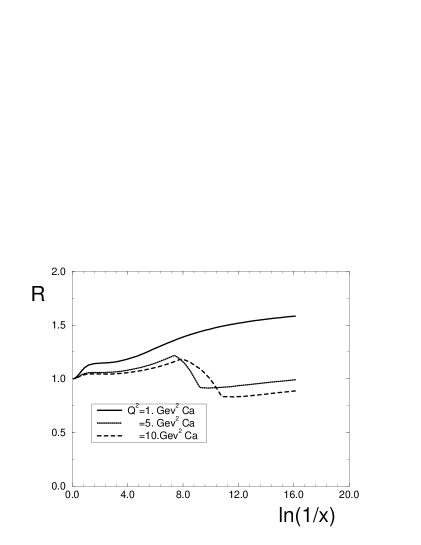
Figure 7: Ratio $xG_{A}^{APPROX}$/ $xG_{A}^{FULL}$.

Eq.(74) is very approximate but Fig.(7) shows that this equations describes the full formula quite well except the region where $Q^{2}\approx Q_{0}^{2}(x)$. The nice feature of this equation is that it illustrates in explicit way how the SC work. First, they provide the new scale for the transverse momentum inside the parton cascade ($Q_{0}(x)$). It means that we expect the GLAP evolution only for distances $r_{t}<1/Q_{0}(x)$. Second, the SC generate the surface term ( the second in Eq.(74) ) which gives $\sigma\propto A^{2/3}$ as for normal hadron nucleus interaction. Of course, all these properties have been anticipated (see Refs.[4, 6, 41]) and Eq.(74) gives the simplest example how they manifest themselves in the case of the deep inelastic scattering.

Now, let us try to understand $x^{\prime}$ dependence of our integrand. In our formula it is implicitly assumed that each gluon can interact with all nucleons in a nucleus. It is not the case because each gluon lives a certain time which is $\tau_{G}=\lambda/mx^{\prime}$ where coefficient $\lambda$ is not quite well known, but $\lambda>1/2$. It means that the gluon can interact only with $T=R^{2}_{A}\rho\tau_{G}$ nucleons unlike $T$ becomes smaller than $A$. Substituting $T$ instead of $A$ we have the following answer for Eq.(72)

$$xG_{A}(x,Q^{2})=\frac{3\alpha_{\rm S}}{\pi}\int_{x}^{1}\frac{dx^{\prime}}{x^{\prime}}T(x^{\prime})\int^{Q^{2}}_{Q_{0}^{2}(x^{\prime})}\frac{dQ^{\prime 2}}{Q^{\prime 2}}x^{\prime}G_{N}^{GLAP}(x^{\prime},Q^{2})$$ (75)

at $x^{\prime}>x_{A}=\lambda/mR_{A}$ we have no log integration over $x^{\prime}$. Therefore, basically, the GLAP equation can be reduced to the form

$$xG_{A}(x,Q^{2})=\frac{3\alpha_{\rm S}A}{\pi}\int_{x}^{x_{A}}\frac{dx^{\prime}}{x^{\prime}}\int^{Q^{2}}_{Q_{0}^{2}(x^{\prime})}\frac{dQ^{\prime 2}}{Q^{\prime 2}}x^{\prime}G_{N}^{GLAP}(x^{\prime},Q^{2})$$ (76)

One can see in Eq.(76) that a new cutoff in $x$ appears in the GLAP equation which has been discussed two decades ago in Ref.[42, 43].

2.8 Theory status of the Mueller formula.

In this section we shall recall the main assumptions that have been made to obtain the Mueller formula.

1. The gluon energy ($x$) should be high (small) enough to satisfy Eqs.(18) and $\alpha_{\rm S}ln(1/x)\leq 1$. The last condition means that we have to assume the leading $ln(1/x)$ approximation of perturbative QCD for the nucleon gluon structure function.

2. The GLAP evolution equations hold in the region of small $x$ or, in other words, $\alpha_{\rm S}ln(1/r^{2}_{t})\leq 1$. One of the lessons from HERA data is the fact that the GLAP evolution can describe the experimental data.

3. Only the fastest partons ($GG$ pairs) interact with the target and there are no correlations (interaction) between partons from the different parton cascades (see Fig.3).

4. There are no correlations between different nucleons in a nucleus.

5. The average $b_{t}$ for $GG$ pair-nucleon interaction is much smaller than $R_{A}$.

The first assumption allows us to treat successive rescatterings as independent and simplifies all formulas reducing the problem to an eikonal picture of the classical propagation of a relativistic particle with high energy ($E\gg\mu^{-1}$, where $\mu$ is the scattering radius in the nuclear matter) through the nucleus. The second one simplifies calculations but we can consider the BFKL evolution [27] instead of GLAP one. The third assumption is artifact of the eikonal approach and we shall discuss it in the following sections. The last two are usual assumptions to treat nucleus scattering. We have used the specific Gaussian parameterization for $b_{t}$ dependence. Also, one can easily generalize our formula in more general case, as Wood-Saxon parameterization [21].

3 pQCD calculations from the Mueller formula.

We use the GRV parameterization [44] for the nucleon gluon distribution, which describes all available experimental data quite well, including recent HERA data at low $x_{B_{j}}$. Moreover, GRV is suited for our purpose because (i) the initial virtuality for the GLAP evolution is small ($Q_{0}^{2}\approx 0.25GeV^{2}$) and we can discuss the contribution of the large distances in MF having some support from experimental data; (ii) in this parameterization the most essential contribution comes from the region where $\alpha_{s}lnQ^{2}\approx 1$ and $\alpha_{s}ln1/x_{B_{j}}\approx 1$. This allows the use of the double leading log approximation of pQCD, where the MF is proven [32]. It should be also stressed here, that we look at the GRV parameterization as a solution of the GLAP evolution equations, disregarding how much of the SC has been taken into account in this parameterization in the form of the initial gluon distribution.

However, in spite of the fact that the GLAP evolution in the GRV parameterization starts from very low virtuality ( $Q^{2}_{0}\,\sim\,0.25GeV^{2}$) it turns out that the DLA still does not work quite well in the accessible kinematic region ($Q^{2}\,>1GeV^{2},x\,>\,10^{-4}$). On the other hand, our master equation (see Eq.64) is proven in DLA. Willing to develop a realistic approach in the region of not ultra small $x$ ($x\,>\,10^{-4})$ we have to change our master equation (64). We suggest to integrate Eq.(67) and substitute the small $x$ kernel for the full GLAP kernel in the first term of the r.h.s. This procedure gives

$$xG_{A}(x,Q^{2})\,\, = \,\,xG_{A}(x,Q^{2})(\,{eq.~{}(\ref{xga2})}\,)\,\,+\,\,AxG^{GRV}_{N}(x,Q^{2})\,\,$$ (77)

$$- \,\,A\,\frac{\alpha_{\rm S}N_{c}}{\pi}\,\int^{1}_{x}\,\int^{Q^{2}}_{Q^{2}_{0}}\,\,\frac{dx^{\prime}}{x^{\prime}}\,\frac{dQ^{\prime 2}}{Q^{\prime 2}}\,x^{\prime}G^{GRV}_{N}(x^{\prime},Q^{\prime 2})\,\,.$$

The above equation includes also $AxG^{GRV}_{N}(x,Q^{2}_{0})$ as the initial condition for the gluon distribution and gives $AxG^{GRV}_{N}(x,Q^{2})$ as the first term of the expansion with respect to $\kappa_{G}$. Therefore, this equation is an attempt to include the full expression for the anomalous dimension for the scattering off each nucleon, while we use the DLA to take into account all SC. Our hope, which we will confirm by numerical calculation, is that the SC are small enough for $x\,>\,10^{-3}$ and we can be not so careful in the accuracy of their calculation in this kinematic region. Going to smaller $x$, the DLA becomes better and eq. (77) tends to our master equation (64).

3.1 The gluon structure function for nucleon.

In this subsection we are going to check how eq. (77) describes the gluon structure function for a nucleon, which is our main ingredient in the Mueller formula. We calculate first the ratio

$$R^{N}_{1}\,\,=\,\,\frac{xG^{A}(x,Q^{2})({eq.~{}(\ref{FINANS})})}{xG^{GRV}_{N}(x,Q^{2})}\,\,,$$ (78)

for $A=1$, which is shown in Fig.8. From this ratio we can see the general behavior of the SC as a function of $ln(1/x)$ and $Q^{2}$. When compared to the GRV gluon distribution, the $xG^{A}$ distribution presents a suppression which increases with $ln(1/x)$ and decreases with the virtuality $Q^{2}$. In the region of the HERA data, $3\,<\,ln(1/x)\,<10$, and $Q^{2}>2\,GeV^{2}$[3], the SC are not bigger than $15\,\%$. The SC give a contribution bigger than $20\,\%$ only at very small value of $x$, where we have no experimental data.

Figure 8: The SC for nucleon (A=1) as a function of $ln(1/x)$ and $Q^{2}$, where ratio $R_{1}$ compares $xG^{A}$ with $xG\,\,(GRV)$ distribution.

In the semiclassical approach (see [1]), the nucleon structure function is supposed to have $Q^{2}$ and $x$ dependence as

$$xG^{N}(x,Q^{2})\,\,\propto\,\,\{Q^{2}\}^{<\gamma>}\,\,\{\frac{1}{x}\}^{<\omega>}\,\,.$$ (79)

We can calculate both exponents using the definitions

$$<\omega>\,\,=\,\,\frac{\partial\ln(xG^{N}(x,Q^{2}))}{\partial\ln(1/x)}\,\,.$$ (80)

$$<\gamma>\,\,=\,\,\frac{\partial\ln(xG^{N}(x,Q^{2}))}{\partial\ln(Q^{2}/Q^{2}_{0})}\,\,;$$ (81)

The eq.(80) gives the average value of the effective power $<\omega>$ of the gluon distribution, $xG(x,Q^{2})\propto x^{-<\omega>}$, which is suitable to study the small $x$ behavior of the gluon distributions. Fig.9 shows the calculation of $<\omega>$ the nucleon distribution calculated using eq.(77) and for GRV gluon distribution, both as functions of $ln(1/x)$ for different values of $Q^{2}$. From the figure, we can see that the effective powers of $xG^{A}(A=1)$ and $xG(GRV)$ have the same general behavior in the small $x$ limit but the nucleon distribution is slightly suppressed.

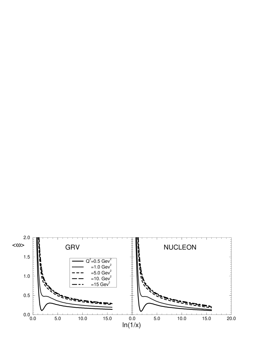
Figure 9: The effective power $<\omega>$ calculated for $xG^{A}(A=1)$ and the GRV distribution.

We calculate also, in the same kinematical region, the exponent $<\gamma>$, given by eq (81). This is the average value of the anomalous dimension, which describes the effective dependence of the distribution in $Q^{2}$ variable. Figs.10 shows $<\gamma>$ for the nucleon and GRV distributions, indicating that the $Q^{2}$ dependence is slightly soften by the SC.

Figure 10: The effective power of $Q^{2}$ dependence calculated for $xG^{A}(A=1)$ and the GRV distribution.

Comparing figures 9 and 10, we can conclude that even these more detailed characteristic of the gluon structure function have not been seriously affected by the SC in the nucleon case.

We also use the GLAP evolution equations to predict the value of the deep inelastic structure function $F_{2}$ from the $xG^{A}$ gluon distribution. Summing the GLAP evolution equations for each quark flavor, the function $F_{2}$ may be written [45]

$$F_{2}=\frac{\alpha_{\rm S}(Q^{2})}{\pi}\sum_{q}e_{q}^{2}\int^{{Q}^{2}}_{{Q}^{2}_{0}}\frac{dQ^{\prime 2}}{Q^{\prime 2}}\int^{1-x}_{0}[z^{2}+(1-z)^{2}]\frac{x}{1-z}G^{N}(\frac{x}{1-z},{Q^{\prime}}^{2})$$ (82)

where the sea quark distributions have been neglected in comparison with the gluon distribution. Fig.11 shows the prediction for $F_{2}$ from $xG^{A}$ and from the GRV distribution, compared with experimental data. As we can see, the magnitude of the suppression due to the SC is less than $10\%$ in the region of the HERA data and this suppression is smaller than the experimental error.

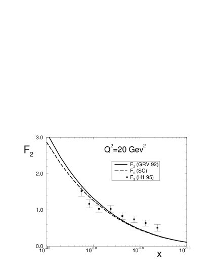
Figure 11: $F_{2}$ from $xG^{A}$ and the GRV distribution, compared with experimental data [3].

From the above results we can conclude that eq. (77) gives a good description for the gluon structure function for nucleon and describes the available experimental data. The MF provides a good description of the SC and can be taken as a correct first approximation in the approach to the nucleus case.

3.2 The gluon structure function for nucleus.

In the framework of perturbative approach it is only possible to calculate the behavior of the gluon distribution at small distances. The initial gluon distribution should be taken from the experiment. Actually the initial virtuality $Q_{0}^{2}$ should be big enough to guarantee that we are dealing with the leading twist contribution. Our main assumption is that we start the QCD evolution with a small value of $Q_{0}^{2}$ considering that the MF is a good model for high twist contributions in DIS off nucleus.

The scale of the SC governs by the value of $\kappa_{A}$, namely they are big for $\kappa_{A}\,>\,$1 and small for $\kappa_{A}\,<\,$ 1. Fig.6 shows the plot of $\kappa_{A}$ = 1 for different nuclei. One can see that the SC should be essential for heavy nuclei starting from Ca at the accessible experimentally kinematic region.

Now we extend the definition of $R_{1}$ for the nucleus case

$$R_{1}\,\,=\,\,\frac{xG^{A}(x,Q^{2})}{AxG^{GRV}_{N}(x,Q^{2})}\,\,,$$ (83)

where the numerator is calculated using eq.(77). Figure 12 shows the results for the calculations of $R_{1}$ as a function of the variables $ln(1/x)$, $lnQ^{2}$ and $A^{1/3}$. Fig.12a presents the ratio $R_{1}$ for two different values of $Q^{2}$ and for different nuclei. The suppression due to the SC increases with $ln(1/x)$ and is much bigger than for the nucleon case. For $A=40$ (Ca) and $Q^{2}=10\,GeV^{2}$, the suppression varies from $4\,\%$ for $ln(1/x)=3$ to $25\,\%$ for $ln(1/x)=10$. For $A=197$ (Au) the suppression is still bigger, going from $6\%$ to $35\%$ in the same kinematic region. Fig. 12b shows the same ratio for different values of $Q^{2}$ for the gold. The suppression decreases with $Q^{2}$. Figs. 12c and d show the $R_{1}$ ratio as a function of $A^{1/3}$ and $x$ for a fixed value of $Q^{2}$. As expected, the SC increases with $A$. An interesting feature of this figure is the fact that the curves tend to straight lines as $x$ increases. It occurs because, as $x$ grows, the structure function $xG(GRV)$ becomes smaller, and the correction term of (77) proportional to $\kappa$ dominates. Since $\kappa$ is proportional to $A^{1/3}$, the curves behave as straight lines. The decrease of suppression with $Q^{2}$ is illustrated in more detail in Figs. 12e and f which presents $R_{1}$ as a function of $\ln Q^{2}$ for different values of $x$ for Ca and Au, respectively. The effect is pronounced for small $Q^{2}$ and $x$ and diminishes as $lnQ^{2}$ increases.

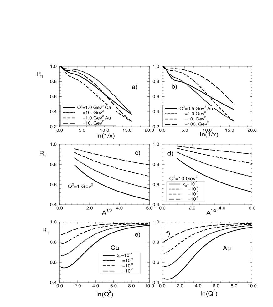
Figure 12: $R_{1}$ as a function of $ln(1/x)$, $lnQ^{2}$ and $A^{1/3}$: a) $R_{1}$ as a function of $ln(1/x)$ for different nucleus and different values of A; b) $R_{1}$ as a function of $lnQ^{2}$ for different values of $x_{B}$ for Au; c) and d) $R_{1}$ as a function of $A^{1/3}$ for different $Q^{2}$; e) and f) $R_{1}$ dependence on $Q^{2}$ for Ca and Au.

Table 1: Values of $R_{1N}$ and $\alpha$ for parameterization $R_{1}\,=\,R_{1N}\,A^{-\,\alpha}$.

	$Q^{2}=1GeV^{2}$		$Q^{2}=10GeV^{2}$
$x$	$R_{1N}$	$\alpha$	$R_{1N}$	$\alpha$
$10^{-2}$	0.94	0.0416	0.98	0.014
$10^{-3}$	0.92	0.0616	0.94	0.034
$10^{-4}$	0.88	0.094	0.92	0.0563
$10^{-5}$	0.8	0.145	0.86	0.093

This picture ( Fig.12 ) shows also that the gluon structure function is far away from the asymptotic one. The asymptotic behavior $R_{1}\,\rightarrow 1$ ( see Figs.12e and f ) occurs only at very high value of $Q^{2}$ as well as in the GLR approach ( see ref. [9] ). The asymptotic $A$-dependence ( $R_{1}\,\propto\,A^{-\frac{1}{3}})$ ) has not been seen in the accessible kinematic range of $Q^{2}$ and $x$ ( see Figs. 12c and d and Table 1 ). This result also has been predicted in the GLR approach [8]. We want also to mention that parameterization $R_{1}\,=\,R_{1N}\,A^{-\alpha}$ does not fit the result of calculations quite well for $1Gev^{2}\,\leq\,Q^{2}\,\leq\,20GeV^{2}$ and $10^{-2}\,\leq\,x\,\leq\,10^{-5}$. For $x\,\sim\,10^{-2}$ the parameterization $R_{1}\,=\,R_{1N}\,-\,R^{\prime}\,A^{\frac{1}{3}}$ with parameters $R_{1N}$ and $R^{\prime}$ for each value of $Q^{2}$, works much better reflecting that only the first correction to the Born term is essential in the Mueller formula.

We extend also the calculation of the exponents $<\omega>$ and $<\gamma>$ of the semiclassical approach for the nuclear case. We calculate the effective power of the nuclear gluon distribution $<\omega>$ using the expression

$$<\omega>\,\,=\,\,\frac{\partial\ln(xG^{A}(x,Q^{2}))}{\partial\ln(1/x)}\,\,.$$ (84)

Fig.13 shows the results as functions of $ln(1/x)$ for different values of $Q^{2}$ and different nucleus. The SC decreases the effective power of the nuclear distribution, giving rise to a flattening of the distribution in the small $x$ region.

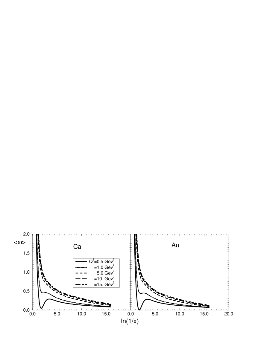
Figure 13: $<\omega>$ for different values of $Q^{2}$ and $A$.

It is also interesting to notice that at small values of $Q^{2}$, the effective power tends to be rather small, even in the nucleon case, at very small $x$. However it should be stressed that the effective power remains bigger than the intercept of the so called ”soft” Pomeron [35], even in the case of a sufficiently heavy nucleus (Au), for $Q^{2}\,>\,1GeV^{2}$. Nowadays, many parameterizations [36] with matching of ”soft” and ”hard” Pomeron have appeared triggered by new HERA data on diffraction dissociation [37]. These parameterization used Pomeron-like behavior namely, $xG(x,Q^{2})\propto x^{-\omega(Q^{2})}$. However, if the Pomeron is a Regge pole, $\omega$ cannot depend on $Q^{2}$, and the only reasonable explanation is to describe $\omega(Q^{2})$ as the result of the SC. Looking at Fig.13 we can claim the SC from the MF cannot provide sufficiently strong SC to reduce the value of $\omega$ to $0.08$, a typical value for the soft Pomeron [35], at least for $Q^{2}\geq 1GeV^{2}$.

The calculation of the effective value of the anomalous dimension $\gamma$ may help us to estimate what distances work in the SC corrections. This effective exponent is given by

$$<\gamma>\,\,=\,\,\frac{\partial\ln(xG^{A}(x,Q^{2}))}{\partial\ln(Q^{2}/Q^{2}_{0})}\,\,.$$ (85)

Figure 14: $<\gamma>$ for different $Q^{2}$ and $A$.

Fig.14 shows the results as functions of $ln(1/x)$ for different values of $Q^{2}$ and for two nuclei. We see that the values of $\gamma$ at $ln(1/x)\,\leq\,5$, for both Ca and Au, is very close to the results for GRV and for nucleon case. At smaller values of $x$, the anomalous dimension presents a sizeable reduction, which increases with A. For $ln(1/x)\,>\,15$, $<\gamma>$ tends to zero unlike in the GLAP evolution equations ( see Fig.10 for the GRV parameterization). Analysing the $Q^{2}$ dependence, we see that $<\gamma>$ is bigger than $1$ only for $Q^{2}=0.5\,GeV^{2}$. For $Q^{2}=1.0\,GeV^{2}$, the anomalous dimension is close to $1/2$, and for $Q^{2}>5.0\,GeV^{2}$ it is always smaller than $1/2$.

Using semiclassical approach, we see that

$$\kappa\propto\frac{1}{Q^{2}}(Q^{2})^{\gamma}\,,$$ (86)

and if $\gamma\geq 1$, the integral over $r_{t}$ in the master equation (77) becomes divergent, concentrating at small distances.

If $1\,>\,\gamma\geq 1/2$, only the first SC term, namely, the second term in expansion of the master equation, is concentrated at small distances, while higher order SC are still sensitive to small $r_{t}$ behavior. Fig.14 shows that this situation occurs for $Q^{2}\,>\,1\,GeV^{2}$, and even for $Q^{2}=1GeV^{2}$ at very small values of $x$. We will return to discussion of these properties of the anomalous dimension behavior in the next section.

In subsection 2.4 we have discussed that the virtual gluon can interact with the target only during the finite time $\tau$ (see eq. (48) ) undergoing $\rho\,\tau\,<\,\rho\,R_{A}$ collisions. In the framework of the Glauber approach the easiest way to take into account the finite life time of the gluon is to include in our calculation the longitudinal part of the transferred momentum ( $q_{z}$ ) to a nucleon during the collision ( see, for example, Ref. [38] ). Using eq. (40) and eq. (47), we can obtain:

$$x\,G_{A}(x,Q^{2})\,\,=\,\,A\,x\,G_{N}(x,Q^{2})\,\,-\,\,A\,\frac{\alpha_{\rm S}\,N_{c}}{\pi}\int^{1}_{x}\,\,\int\,\frac{dx^{\prime}}{x^{\prime}}\,\frac{dQ^{\prime 2}}{Q^{\prime 2}}\,\,L(q_{z})\,\,x^{\prime}\,G_{N}(x^{\prime},Q^{\prime 2})$$ (87)

$$+\,\,\frac{2R^{2}_{A}}{\pi^{2}}\,\int^{1}_{x}\,\frac{dx^{\prime}}{x^{\prime}}\,\int^{\frac{1}{Q^{2}_{0}}}_{\frac{1}{Q^{2}}}\,\frac{dr^{2}_{t}}{r^{4}_{t}}\,\,\{\,C\,+\,\ln(L(q_{z})\,\kappa_{G}(x^{\prime},r^{2}_{t}))+\,\,E_{1}(L(q_{z})\,\kappa_{G}(x^{\prime},r^{2}_{t})\,)\}\,\,.$$

where

$$L(q_{z})\,\,=\,\,e^{-\,\frac{R^{2}_{A}}{4}\,m^{2}\,(x\,+\,x^{\prime})^{2}}\,\,.$$

Fig. 15 shows the result of our calculations. Comparing Fig.12 with this picture, one can see that the finite life time of the virtual gluon affects the behavior of the gluon structure function only at sufficiently large $x$ ( $x\,\geq\,10^{-2}$ ) diminishing the value of the SC in this kinematic region. More interested in the small $x$ behavior of the gluon structure function in nuclei we neglect the finite life time of a gluon through all calculations below.

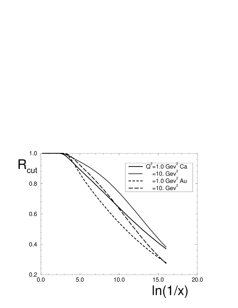
Figure 15: $R_{1}$ for CA and Au with gluon life time cutoff.

3.3 The behavior of $\alpha_{s}$.

We calculated the ratio

$$\frac{<\alpha_{\rm S}^{A}>}{<\alpha_{\rm S}^{N}>}=\frac{xG^{GLAP}_{N}(x,Q^{2})}{xG_{A}(x,Q^{2})}\frac{\left[\frac{\partial}{\partial\ln\frac{1}{x}\partial\ln Q^{2}}(xG_{A}(x,Q^{2}))\right]}{\left[\frac{\partial}{\partial\ln\frac{1}{x}\partial\ln Q^{2}}(xG^{GLAP}_{N}(x,Q^{2}))\right]}\,,$$ (88)

Figure 16: The ratio $<\alpha_{\rm S}^{A}>/<\alpha_{\rm S}^{GRV}>$.

which is equal to $1$ in the case of the GLAP equation. In some sense it characterizes the value of the effective QCD coupling constant in a nucleus. This constant becomes smaller due to SC and in a restricted kinematic region we can treat the parton cascade as a parton system evolving according to the linear GLAP equations but with smaller coupling constant. The result is shown in Fig.16. The physical meaning of the weakening of the coupling constant is very simple. At low-$x$, the gluon density increases and in a typical parton cascade cell there are many partons with different colors. The color average gives smaller mean color charge at small gluon densities. One manifestation of the parton interaction weakening is the bigger value of $\Lambda$ QCD for nuclei at small $x$. From Fig.16 one can see that the GLAP evolution equation can be used to describe the evolution of the gluon structure function for the nucleon in HERA kinematic region ( $x\,>\,10^{-4}$ ) but only for sufficiently large photon virtualities ( $Q^{2}\,\geq\,5\,GeV^{2}$ ). At smaller values of $Q^{2}$ we have to develop more sophisticated approach for the adequate treatment. In the case of nuclei, the GLAP evolution equations with screened ( reduced ) value of $\alpha_{\rm S}$ could be considered only as the first rough approximation even for large $Q^{2}$ ( $Q^{2}\,\geq\,5\,GeV^{2}$ ).

4 Beyond the Glauber Approach.

In this section we discuss the corrections to the Glauber approach (the Mueller formula of Eq.(66) ) as well as the way to construct a complete theory for deep inelastic scattering off a nucleus.

4.1 The second iteration of the Mueller formula.

To understand how big could be the corrections to the Glauber approach we calculate the second iteration of the Mueller formula of Eq.(66). As has been discussed, Eq.(66) describes the rescattering of the fastest gluon ( gluon - gluon pair ) during the passage through a nucleus ( see Figs. 1 and 2 ). In the second iteration we take into account also the rescattering of the next to the fastest gluon. This is a well defined task due to the strong ordering in the parton fractions of energy in the parton cascade in leading $ln(1/x)$ approximation of pQCD that we are dealing with. Namely:

$$x_{B}\,\,<\,\,x_{n}\,\,<\,\,...\,\,<x_{1}\,\,<\,\,1\,\,;$$ (89)

where 1 corresponds to the fastest parton in the cascade.

Therefore, in the second interaction we include the rescatterings of the gluons with the energy fraction $1$ and $x_{1}$ ( see Fig.5 ). Doing the first iteration we insert in Eq.(66) $G_{N}(x,Q^{2})\,=\,G^{GRV}_{N}(x,Q^{2})$. For the second iteration we calculate the gluon structure function using Eq.(66) substituting

$$x\,G_{N}\,\,=\,\,\frac{xG^{1}_{A}(x,Q^{2})}{A}\,\,-\,\,x\,G^{GRV}_{N}(x,Q^{2})\,\,;$$ (90)

where $xG^{1}_{A}$ is the result of the first iteration of Eq.(66) that has been discussed in details in section 3.

Fig.17 shows the need to subtract $xG^{GRV}_{N}$ in eq. (90) making the second iteration. Indeed, in the second iteration we take into account the rescattering of gluon $1^{\prime}$ - gluon $2^{\prime}$ pair off a nucleus. We picture in Fig.16 the first term of such iteration in which $G_{1^{\prime}}G_{2^{\prime}}$ pair has no rescatterings. It is obvious that it has been taken into account in our first iteration, so we have to subtract it to avoid a double counting.

Figure 17: The first term of the second iteration of eq. (90).

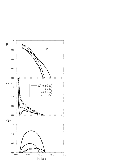
Figure 18: Second iteration calculations for $R_{1}$, $<\omega>$, and $<\gamma>$ for Ca and Au.

One can see in Figs.18 that the second iteration gives a big effect and changes crucially $R_{1}$, $<\gamma>$, and $<\omega>$. The most remarkable feature is the crucial change of the value of the effective power $\omega(Q^{2})$ for the “Pomeron” intercept which tends to zero at HERA kinematic region, making possible the matching with “soft” high energy phenomenology. It is also very instructive to see how the second iteration makes more pronounced all properties of the behavior of the anomalous dimension ( $<\gamma>$) that we have discussed. The main conclusions which we can make from Figs.18 are: (i) the second iteration gives a sizable contribution in the region $x\,\,<\,\,10^{-2}$ and for $x\,\,\leq\,\,10^{-3}$ it becomes of the order of the first iteration; (ii) for $x\,\,<\,\,10^{-3}$ we have to calculate the next iteration. It means that for such small $x$ we have to develop a different technique to take into account rescatterings of all the partons in the parton cascade which will be more efficient than the simple iteration procedure for Eq.(66). However, let us first understand why the second iteration becomes essential to establish small parameters that enter to our problem.

4.2 Parameters of the pQCD approach.

As has been discussed, we use the GLAP evolution equations for gluon structure function in the region of small $x$. It means, that we sum the Feynman diagrams in pQCD using the following set of parameters:

$$\alpha_{\rm S}\,\,\ll\,\,1\,\,;\,\,\,\,\,\,\,\,\,\,\alpha_{\rm S}\,\ln\frac{1}{x}\,\,<\,\,1\,\,;\,\,\,\,\,\,\,\,\,\,\alpha_{\rm S}\,\ln\frac{Q^{2}}{Q^{2}_{0}}\,\,<\,\,1\,\,;\,\,\,\,\,\,\,\,\,\,\alpha_{\rm S}\,\,\ln\frac{Q^{2}}{Q^{2}_{0}}\,\,\ln\frac{1}{x}\,\,\approx\,\,1\,\,.$$ (91)

The idea of the theoretical approach of rescattering that has been formulated in the GLR paper [1] is to introduce a new parameter :

$$\kappa\,\,=\,\,\frac{N_{c}\,\alpha_{\rm S}\,\pi\,A}{2\,Q^{2}\,R^{2}_{A}}\,xG(x,Q^{2})$$ (92)

and sum all Feynman diagrams using the set of eq. (91) and $\kappa$ as parameters of the problem, neglecting all contributions of the order of: $\alpha_{\rm S}$, $\alpha_{\rm S}\,\kappa$, $\alpha_{\rm S}\ln(1/x)$, $\alpha_{\rm S}\ln(1/x)\,\kappa$, $\alpha_{\rm S}\ln(Q^{2}/Q^{2}_{0})$ and $\alpha_{\rm S}\ln(Q^{2}/Q^{2}_{0})\,\kappa$. It should be stressed that Mueller formula gives a solution for such approach. Indeed, Eq.(66) depends only on $\kappa$ absorbing all
$(\,\alpha_{\rm S}\,\ln(Q^{2}/Q^{2}_{0})\,\ln(1/x)\,)^{n}$ contributions in $xG(x,Q^{2})$. However, it is not a complete solution. To illustrate this point let us compare the value of the second term of the expansion of Eq.(62) with respect to $\sigma(r^{2}_{t})$ with the first correction due to the second iteration in the first term of such an expansion. In other words we wish to compare the values of the diagrams in Fig.18a and Fig.18b. The contribution of the diagram of Fig.18a is equal:

$$\Delta xG(x,Q^{2})\,(\,Fig.18a\,)\,\,=\,\,\frac{R^{2}_{A}}{2\,\pi^{2}}\,\,\int\frac{dx^{\prime}}{x^{\prime}}\,\int\,dQ^{\prime 2}\,\,\kappa^{2}(x^{\prime},\frac{Q^{\prime 2}}{4})\,\,,$$ (93)

where $x^{\prime}$ and $Q^{\prime 2}$ are the fraction of energy and the virtuality of gluon $1$ in Fig.18a.

The diagram of Fig.18b contains one more gluon and its contribution is:

$$\Delta xG(x,Q^{2})\,(\,Fig.18b\,)\,\,=\,\,\frac{R^{2}_{A}}{\pi^{2}2}\,\,\frac{N_{c}\alpha_{\rm S}}{\pi}\int\,\,\frac{dx^{\prime}}{x^{\prime}}\,\,\frac{dQ^{\prime 2}}{Q^{\prime 2}}\,\,\int\frac{dx"}{x"}\,\int\,dQ"^{2}\,\,\kappa^{2}(x",\frac{Q"^{2}}{4})$$

$$\propto\,\,\frac{\alpha_{\rm S}N_{c}}{\pi}\,\,\ln(1/x)\,\,\ln(Q^{2}/Q^{2}_{0})\,\,\Delta xG(x,Q^{2})(\,Fig.18a\,)\,\,,$$ (94)

where $x^{\prime}$ ($x^{\prime\prime}$) and $Q^{\prime 2}$ ( $Q^{\prime\prime 2}$) are the fraction of energy and the virtuality of gluon $1$ ($1^{\prime}$) respectively in Fig.18b.

Figure 19: Corrections to the Glauber approach.

Therefore, eq. (94) gives the contribution which is of the order of eq. (93) in the kinematic region where the set of parameters of eq. (91) holds. It means also that we need to sum all diagrams of Fig.18b type to obtain the full answer. In the diagram of Fig. 18b not only one but many gluons can be emitted. Such emission leads to so called “triple ladder” interaction, pictured in Fig.18c ( see ref.[1] ). This diagram is the first from so called “fan” diagrams of Fig. 18d. To sum them all we can neglect the third term in Eq.(65) and treat the remained terms as an equation for $xG(x,Q^{2})$. It is easy to recognize that we obtain the GLR equation [1][7]. Generally speaking the GLR equation sums the most important diagrams in the kinematic region where $\alpha_{\rm S}\,\ln(1/x)\,\ln(Q^{2}/Q^{2}_{0})\,\,\gg\,\,1$ and $\kappa\,<\,1$. Using the Mueller formula we can give more precise estimates for the kinematic region where we can trust the GLR equation. Indeed, in Fig.19 we plot the ratio

$$R_{C}\,\,=\,\,\frac{\frac{R^{2}_{A}}{\pi^{2}2}\,\,\int\frac{dx^{\prime}}{x^{\prime}}\,\int\,dQ^{\prime 2}\,\,\kappa^{2}(x^{\prime},\frac{Q^{\prime 2}}{4})}{xG_{A}(x,Q^{2})(\,\,Eq.(75)\,\,)\,\,-\,\,A\,x\,G^{GRV}_{N}(x,Q^{2})}\,\,.$$ (95)

If $R_{C}$ = 1, all the SC can be evaluated within good accuracy by the second term in Eq.(65).

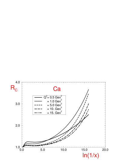
Figure 20: The ratio $R_{C}$ as a function of $ln(1/x)$ and $Q^{2}$.

From Fig.20 one can see that for Ca we can safely restrict by the second term in the master equation and use the GLR equation to take into account the interaction of all parton in the parton cascade even for low values of $Q^{2}$ in the HERA kinematic region ($x\,>\,10^{-5}$). However, for the nuclei we have to develop more general procedure for the interaction of the Mueller formula than the GLR equation for $x\,<\,10^{-2}$.

We need to make some very important remarks, concerning the whole approach based on the Glauber - type shadowing corrections. It has been proven [46][47] that keeping all parameters of eq. (90) and eq. (91) and summing all Glauber - type interactions, as the Mueller formula does, is not enough. It turns out that the interaction between partons from different parton cascades that interact with the different nucleons are important. Fig.20a shows the first interaction of such a type that has to be taken into account. This diagram should be compared with Fig.20b which shows the interaction included in the Mueller formula as well as in the GLR equation. Fortunately, these new contributions are proportional to $\frac{1}{N^{2}_{c}}$ and we will neglect them, considering $N_{c}$ is large enough. The general procedure how to sum all corrections of the order of $\frac{1}{N^{2}_{c}}$ at least for the GLR equation has been developed in ref. [40]. In spite of the small parameter $\frac{1}{N^{2}_{c}}$ the parton selfinteraction can be essential for the case of a nuclear target but we postpone the detailed discussion of this problem to future publication.

Figure 21: The Glauber approach ( Fig.20b) and corrections to the Glauber approach due to interaction between partons from different parton cascades.

4.3 The GLR equation for nucleus.

In this subsection we are going to discuss the GLR equation as a way of taking into account the interaction of all partons in the parton cascade with the target in spite of the criticism of the previous section. Indeed, let us go back to the discussion of the behavior of the average anomalous dimension in the Mueller formula and in the first iteration of the MF ( see Figs.14 and 19). The general feature of the both iterations is the fact that the resulting value of the anomalous dimension ( $<\gamma>$ ) turns out to $<\gamma>\,\leq\,\frac{1}{2}$ for $Q^{2}\,\geq\,1GeV^{2}$. In this case the high order terms in the expansion of the MF are concentrated at large distances while the second one can be divergent at small distances if $<\gamma>\,\rightarrow\,\frac{1}{2}$. Therefore we can rewrite the Mueller formula in the form:

$$xG_{A}(x,Q^{2})\,=\,\frac{4}{\pi^{2}}\,\int^{1}_{x}\,\frac{dx^{\prime}}{x^{\prime}}\,\int^{\infty}_{0}d\,b^{2}_{t}$$ (96)

$$\{\int^{\frac{4}{Q^{2}_{0}}}_{\frac{4}{Q^{2}}}\,\,\frac{d^{2}r_{t}}{\pi\,r^{4}_{t}}\,2\,[\,1\,-\,e^{-\frac{1}{2}\sigma^{GG}_{N}(x^{\prime},r^{2}_{t})S(b^{2}_{t})}\,]\,\,+\,\,\int^{\infty}_{\frac{4}{Q^{2}_{0}}}\,\,\frac{d^{2}r_{t}}{\pi\,r^{4}_{t}}\,2\,[\,1\,-\,e^{-\frac{1}{2}\sigma^{GG}_{N}(x^{\prime},r^{2}_{t})S(b^{2}_{t})}\,]\,\}\,\,,$$

where $Q_{0}$ we choose of the order of 1 $GeV^{2}$. Recalling that $<\gamma>\,<\,1$ we can expand the first integral in eq. (96) and neglect all high contribution except the second term which can be important in the region where $<\gamma>\,\rightarrow\,\frac{1}{2}$. Differentiating with respect to $\ln Q^{2}$ and $\ln(1/x)$ one obtain the GLR equation, namely

$$\frac{\partial^{2}xG_{A}(x,Q^{2})}{\partial\ln(1/x)\,\partial\ln Q^{2}}\,\,=\,\,\frac{N_{c}\alpha_{\rm S}}{\pi}\,xG_{A}(x,Q^{2})\,\,-\,\,\frac{\alpha_{\rm S}^{2}A^{2}}{2R^{2}_{A}}\,\left(\,xG_{A}(x,Q^{2})\,\right)^{2}\,\,.$$ (97)

The second integral in eq. (96) gives the initial condition for the GRL equation. We want to draw your attention to two important outcomes from this simple consideration. First, the initial condition should be set only at sufficiently large value of $Q^{2}$, e.g., at $Q^{2}=Q^{2}_{0}\,\geq\,1GeV^{2}$. Second, we cannot use the MF to calculate this initial condition for the nucleus using the nucleon gluon structure function, since the corrections to MF for $Q^{2}\,\leq 1GeV^{2}$ is large. Therefore, the solution of the GLR equation is only reliable in a kinematic region where it does not depend on any initial distribution. The way out of this shortcoming is only to use the direct information on the gluon structure function in a nucleus. Therefore, in such approach the main advantage of the Glauber formula is lost: the possibility to calculate the nucleus structure function from the nucleon one. This is the reason to develop a more general approach in the next subsection.

4.4 The generalization of the Glauber Approach.

We suggest the following way to take into account the interaction of all partons in a parton cascade with the target. Let us differentiate the Mueller formula over $y\,=\,\ln(1/x)$ and $\xi=\ln(Q^{2}/Q^{2}_{0})$. It gives:

$$\frac{\partial^{2}xG_{A}(y,\xi)}{\partial y\partial\xi}\,\,=\,\,\frac{2\,R^{2}_{A}\,\,Q^{2}}{\pi^{2}}\,\,\{\,\,C\,\,+\,\,\ln\kappa\,\,+\,\,E_{1}(\kappa)\,\,\}\,\,.$$ (98)

Rewriting eq. (98) in terms of $\kappa$ given by

$$\kappa\,\,=\,\,\frac{N_{c}\alpha_{\rm S}}{2Q^{2}R^{2}_{A}}\,xG_{A}(x,Q^{2})$$ (99)

we obtain:

$$\frac{\partial^{2}\kappa(y,\xi)}{\partial y\partial\xi}\,\,+\,\,\frac{\partial\kappa(y,\xi)}{\partial y}\,\,=\,\,\frac{N_{c}\,\alpha_{\rm S}\,}{\pi}\,\,\{\,\,C\,\,+\,\,\ln\kappa(y,\xi)\,\,+\,\,E_{1}(\kappa(y,\xi))\,\,\}\,\,\equiv\,\,F(\kappa)\,\,.$$ (100)

Now, let us consider the expression of eq. (100) as the equation for $\kappa$. This equation sums all contributions of the order $(\,\alpha_{\rm S}\,y\,\xi\,)^{n}$ absorbing them in $xG_{A}(y,\xi)$, as well as all contributions of the order of $\kappa^{n}$. For $N_{c}\,\rightarrow\,\infty$ eq. (100) gives the complete solution to our problem. The great advantage of this equation in comparison with the GLR one is the fact that it describes the region of large $\kappa$ and provides the correct matching both with the GLR equation and with the Glauber ( Mueller ) formula in the kinematic region where $\alpha_{\rm S}y\xi\,\leq\,1$.

Eq. (100) is the second order differential equation in partial derivatives and we need two initial ( boundary ) conditions to specify the solution. The first one is obvious, namely, at fixed $y$ and $Q^{2}\,\rightarrow\,\infty$

$$\kappa\,\,\rightarrow\,\,\frac{N_{c}\,\alpha_{\rm S}\,\pi\,A}{2\,Q^{2}\,R^{2}_{A}}\,xG^{GLAP}_{N}(x,Q^{2})\,\,.$$

The second one we can fix in the following way: at $x=x_{0}\,\,(y=y_{0})$ which is small, namely, in the kinematic region where $\alpha_{\rm S}y\xi\,\leq\,1$

$$\kappa\,\,\rightarrow\,\,\kappa_{in}\,\,=\,\,\frac{N_{c}\,\alpha_{\rm S}\,\pi}{2\,Q^{2}\,R^{2}_{A}}\,xG_{A}(x,Q^{2})\,\,,$$ (101)

where $xG_{A}$ is given by the Mueller formula ( see Eq.(66) ). Practically, we can take $x_{0}\,=\,10^{-2}$, because corrections to the MF are small at this value of $x=x_{0}$.

4.5 The solution to the generalized evolution equation.

4.5.1 The asymptotic solution

First observation is the fact that eq. (100) has a solution which depends only on $y$. Indeed, one can check that $\kappa\,=\,\kappa_{asymp}(y)$ is the solution of the following equation:

$$\frac{d\kappa_{asymp}}{dy}\,\,=\,\,F(\,\kappa_{asymp}\,)\,\,.$$ (102)

The solution to the above equation is:

$$\int^{\kappa_{asymp}(y)}_{\kappa_{asymp}(y=y_{0})}\,\,\frac{d\kappa^{\prime}}{F(\kappa^{\prime})}\,\,=\,\,y-y_{0}\,\,.$$ (103)

It is easy to find the behavior of the solution to eq. (103) at large value of $y$ since $F(\kappa)\,\,\rightarrow\,\,\bar{\alpha}_{\rm S}\ln\kappa$ at large $\kappa$ ( $\bar{\alpha}_{\rm S}=\frac{N_{c}}{\pi}\,\alpha_{\rm S}$ ). It gives

$$\kappa_{asymp}\,\,\rightarrow\,\,\bar{\alpha}_{\rm S}y\,\ln(\bar{\alpha}_{\rm S}y)\,\,\,\,\,\,at\,\,\,\,\,\,\,\bar{\alpha}_{\rm S}y\,\,\gg\,\,1\,\,.$$ (104)

At small value of $y$, $F(\kappa)\,\,\rightarrow\,\,\bar{\alpha}_{\rm S}\kappa$ and we have:

$$\kappa_{asymp}\,\,\rightarrow\,\,\kappa_{asymp}(y=y_{0})\,\,e^{\bar{\alpha}_{\rm S}(y-y_{0})}\,\,.$$ (105)

The solution is given in Fig.22 for $\bar{\alpha}_{\rm S}=1/4$ in the whole region of $y$ for different nuclei in comparison with our calculations based on the MF. We chose the value of $\kappa_{asymp}(y=y_{0})$ from eq. (101). We claim this solution is the asymptotic solution to eq. (100) and will argue on this point a bit later.The calculations in Glauber approach for nucleon overshoot the asymptotic solution at large values of $Q^{2}$ in HERA kinematic region ( at $x\,<\,10^{-2}$ ). However, at small values of $Q^{2}$ the Glauber approach leads to stronger SC than the asymptotic solution. For nuclei the SC incorporated in the asymptotic solution turn out to be much stronger than the SC in the Glauber approach for any $Q^{2}\,>\,1\,GeV^{2}$ at $x\,>\,10^{-2}$. In this kinematic region the solution of eq. (100) is drastically different from the Glauber one.

A general conclusion for Fig.22 is very simple: the amount of shadowing which was taken into account in the MF is not enough , at least for the gluon structure function in nuclei at $x\,<\,10^{-2}$ and we have to solve eq. (100) to obtain the correct behavior of the gluon structure function for nuclei.

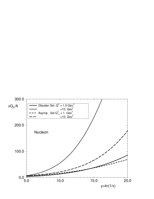
Figure 22: The Glauber approach and asymptotic solution for different nuclei.

Now, we would like to show that solution eq. (100) is the asymptotic solution of the new evolution equation. In order to check this let us try to find the solution to eq. (100) in the form $\kappa\,=\,\kappa_{asymp}\,+\,\Delta\kappa$, anticipating that $\Delta\kappa$ is small. If it is so, the following linear equation can be written for $\Delta\kappa$:

$$\frac{\partial^{2}\Delta\kappa(y,\xi)}{\partial y\,\partial\xi}\,\,+\,\,\frac{\partial\Delta\kappa(y,\xi}{\partial y}\,\,=\,\,\frac{dF(\kappa)}{d\kappa}\,|_{\kappa=\kappa_{asymp}(y)}\,\,\Delta\kappa(y,\xi)\,\,.$$ (106)

The general solution to eq. (106) one can find going to the Mellin transform in respect to $\xi$, namely:

$$\Delta\kappa(y,\xi)\,\,=\,\,\int_{C}\,\,\frac{d\nu}{2\,i\,\pi}\Delta\kappa(y,\nu)\,\,e^{\nu(\,\xi\,-\,\xi_{0}\,)}\,\,,$$ (107)

where contour $C$ is taken to the right of all singularities in $\nu$ for function $\Delta\kappa(y,\nu)$.

For function $\Delta\kappa(y,\nu)$ we have the equation:

$$(\,\nu\,\,+\,\,1\,)\,\frac{d\Delta\kappa(y,\nu)}{dy}\,\,=F^{\prime}(y)\Delta\kappa(y,\nu)\,\,,$$ (108)

where we denote $F^{\prime}(y)\,\,=\frac{dF(\kappa)}{d\kappa}\,|_{\kappa=\kappa_{asymp}(y)}$. Solving eq. (108) we obtain the answer:

$$\Delta\kappa(y,\xi)\,\,=\,\,\int_{C}\,\,\frac{d\nu}{2\,i\,\pi}\Delta\kappa(\nu)\,\,\exp[\,\nu(\xi\,-\xi_{0})\,+\,\,\frac{1}{\nu+1}\,\int^{y}_{y_{0}}F^{\prime}(y^{\prime})dy^{\prime}\,]\,\,=$$ (109)

$$\,\,=\,\,\int_{C}\,\,\frac{d\nu}{2\,i\,\pi}\Delta\kappa(\nu)\,\,\exp[\,\nu(\,\xi\,-\,\xi_{0}\,)\,\,+\,\,\frac{1}{\nu+1}\,\ln(F(\kappa_{asymp}(y))\,\,,$$

where function $\Delta\kappa(\nu)$ should be find from the initial condition at $\xi=\xi_{0}$, namely $\Delta\kappa(y,\xi=0)$ = 0.

To satisfy the initial condition we will find function $\Delta\kappa(\nu)$ from the equation:

$$\kappa_{asymp}(y,\xi=\xi_{0})\,\,=\,\,\int_{C}\,\,\frac{d\nu}{2\,i\,\pi}\Delta\kappa(\nu)\,\,\exp[\,\,\frac{1}{\nu+1}\,\int^{y}_{y_{0}}F^{\prime}(y^{\prime})dy^{\prime}\,]\,\,.$$ (110)

In doing so we obtain $\Delta\kappa(y,\xi)$:

$$\Delta\kappa(y,\xi)\,\,=\,\,\int_{C}\,\,\frac{d\nu}{2\,i\,\pi}\Delta\kappa(\nu)\,\,\exp[\,\,\frac{1}{\nu+1}\,\int^{y}_{y_{0}}F^{\prime}(y^{\prime})dy^{\prime}\,]\,\,\{\,\exp(\,\nu(\xi-\xi_{0})\,)\,\,-\,\,1\,\}\,\,,$$ (111)

which satisfies all our requirements.

We claim that function:

$$\kappa(y,\xi)\,\,=\,\,\int_{C}\,\,\frac{d\nu}{2\,i\,\pi}\Delta\kappa(\nu)\,\,\exp[\,\,\frac{1}{\nu+1}\,\int^{y}_{y_{0}}F^{\prime}(y^{\prime})dy^{\prime}\,]\,\,\exp(\,\nu(\xi-\xi_{0})\,)\,\,$$ (112)

is the approximate solution to the nonlinear equation (100).

Let us check this point considering very large values of $\xi$ and $y$. In the region of large $y$, $\int^{y}_{y_{0}}F^{\prime}(y^{\prime})dy^{\prime}\,\,\rightarrow\,\,\bar{\alpha}_{\rm S}\ln(\bar{\alpha}_{\rm S}y)$ and $\Delta\kappa(\nu)\,\,\propto\,\,\frac{1}{\nu}$ which reproduces $\kappa_{asymp}\,\,\rightarrow\,\,\bar{\alpha}_{\rm S}y$ at large $y$ and $\xi=\xi_{0}$. Making use of the saddle point approximation one can see that

$$\Delta\kappa(y,\xi)\,\,\rightarrow\,\,e^{2\sqrt{\xi\alpha_{\rm S}\ln(bar\alpha_{\rm S}y)}}\,\,\ll\,\,\kappa_{asymp}\,\,.$$ (113)

To give a solution able to describe the experimental data we have to adjust the behavior of $\kappa_{asymp}$ at small $y$ ( $y\,<\,y_{0}$ ) with the available parameterization of the gluon structure function, in particular with the GRV parameterization which we have been using through this paper as a standard one. We have not done this job in this paper and we are going to publish the result of this calculation elsewhere. However, to estimate the effect of the SC which follow from eq. (100) we solve this equation using the semiclassical approach.

4.5.2 Semiclassical Approach

Here we solve eq.(100) using the semiclassical approach, adjusted to the solution of the nonlinear equation of eq.(100)-type in refs. [1, 48, 49]. For simplicity, we assume that $\alpha_{\rm S}$ is fixed.

In the semiclasical approach we are looking for the solution of eq. (100) in the form

$$\kappa=e^{S}$$ (114)

where $S$ is a function with partial derivatives: $\frac{\partial S}{\partial y}=\omega$ and $\frac{\partial S}{\partial\xi}=\gamma$ which are smooth function of $y$ and $\xi$. It means that

$$\frac{\partial^{2}S}{\partial\xi\partial y}\ll\frac{\partial S}{\partial y}\cdot\frac{\partial S}{\partial\xi}=\omega\gamma$$ (115)

Using eq.(115), one can easily rewrite eq.(100) in the form

$$\frac{\partial S}{\partial y}\frac{\partial S}{\partial\xi}+\frac{\partial S}{\partial y}=e^{-S}F(e^{S})\equiv\Phi(S)$$ (116)

or

$$\omega(\gamma+1)=\Phi(S)$$ (117)

We are going to use the method of characteristics( see, for example, ref.[51]). For equation in the form

$$F(\xi,y,S,\gamma,\omega)=0$$ (118)

we can introduce the set of characteristic lines $(\xi(t),y(t),S(t),\omega(t),\gamma(t))$, functions of the variable $t$, which satisfy the following equations

$$\frac{d\xi}{dt}=F_{\gamma}\,;\,\,\frac{dy}{dt}=F_{\omega}\,;\,\,\frac{dS}{dt}=\gamma F_{\gamma}+\omega F_{\omega}\,;\,\,$$

$$\frac{d\gamma}{dt}=-(F_{\xi}+\gamma F_{S})\,;\,\,\frac{d\omega}{dt}=-(F_{y}+\omega F_{S})$$ (119)

where $F_{\xi}=\frac{\partial}{\partial\xi}F(\xi,y,S,\gamma,\omega)$ etc. Eq.(119) looks as follows for the case of eq(117)

$$\frac{d\xi}{dt}=\omega\,;\,\,\frac{dy}{dt}=\gamma+1\,;\,\,\frac{dS}{dt}=\omega(2\gamma+1)\,;\,\,$$

$$\frac{d\gamma}{dt}=\Phi^{\prime}_{S}\gamma\,;\,\,\frac{d\omega}{dt}=\Phi^{\prime}_{S}\omega\,\,,$$ (120)

where $\Phi^{\prime}_{S}=\frac{\partial\Phi}{\partial S}$. For practical purpose it is better to rewrite the set of equations(120) in the form

$$\frac{d\xi}{dy}=\frac{\omega}{\gamma+1}\,;\,\,\,\frac{dS}{dy}=\omega\frac{(2\gamma+1)}{\gamma+1}\,;\,\,\frac{d\gamma}{dy}=\Phi^{\prime}_{S}\frac{\gamma}{\gamma+1}\,.$$ (121)

Using eq.(117), eq.(121) can be rewritten

$$\frac{d\xi}{dy}=\frac{\Phi(S)}{(\gamma+1)^{2}}\,;\,\,\,\,\,\frac{dS}{dy}=\frac{2\gamma+1}{(\gamma+1)^{2}}\Phi(S)\,;\,\,\,\,\frac{d\gamma}{dy}=\Phi^{\prime}_{S}\frac{\gamma}{\gamma+1}\,.$$ (122)

The initial condition for this set of equations we derive from eq.(101), namely

$$S_{0}=ln\kappa_{in}(y_{0},\xi_{0})$$

$$\gamma_{0}=\left.\frac{\partial ln\kappa_{in}(y_{0},\xi)}{\partial\xi}\right|_{\xi=\xi_{0}}$$ (123)

Let us discuss the main properties of the solution before numerical calculations. The first observation is that $\Phi^{\prime}_{S}<0$ and $\Phi(S)>0$ for all values of $S$. From the second equation of the set (122) we see that $S$ decreases along all trajectories with $\gamma<-1/2$ and increases for trajectories with $\gamma>-1/2$. Thus, it is useful to study the qualitative behavior of the trajectories for two different regions of the initial condition. Namely, for $\gamma_{0}<-1/2$ and for $\gamma_{0}>-1/2$.

From the third equation of the set (122), we notice that $\frac{d\gamma}{dy}\,>\,0$ for all $\gamma<0$. It means that $\gamma$ grows with $y$ starting from $\gamma_{0}$. However for $\gamma>0$, $\frac{d\gamma}{dy}<0$ and $\gamma$ starts to fall down. In both cases, for $\gamma_{0}>-1/2$, $S$ goes to infinity as $y$ grows, and $\Phi^{\prime}_{S}$ and the derivative $\frac{d\gamma}{dy}$ go to zero. Thus, we can conclude that $\gamma\rightarrow 0$ as $y\rightarrow\infty$.

It is useful to study closer what is happening at small $\gamma$.

From equations (122), we can write

$$\frac{dS}{d\gamma}=\frac{2\gamma+1}{\gamma(\gamma+1)}\frac{\Phi(S)}{\Phi^{\prime}_{S}(S)}$$ (124)

or

$$\frac{dln\Phi}{d\gamma}=\frac{2\gamma+1}{\gamma(\gamma+1)}$$ (125)

which has the solution

$$\Phi(S)=\Phi(S_{0})\left(\frac{\gamma(\gamma+1)}{\gamma_{0}(\gamma_{0}+1)}\right)\,.$$ (126)

For small $|\gamma|$ the solution of eq.(126) is correlated with large values of $S$, since $\Phi(S)$ has maximum at $S=S_{0}$ and decreases at $S>S_{0}$. On the other hand, at large $S$, $\Phi^{\prime}_{S}\rightarrow-\Phi(S)$. Substituting this relation in the third equation of (122), we obtain

$$\frac{d(\gamma/\gamma_{0})}{dy}=-\frac{\Phi(S_{0})}{\gamma_{0}+1}\frac{\gamma^{2}}{\gamma_{0}^{2}}\,,$$ (127)

which solution is

$$-\frac{1}{\gamma/\gamma_{0}}+1=-\frac{\Phi(S_{0})}{\gamma_{0}+1}(y-y_{0})$$ (128)

or

$$\frac{\gamma}{\gamma_{0}}=\frac{1}{\frac{\Phi(S_{0})}{\gamma_{0}+1}(y-y_{0})+1}\,.$$ (129)

Therefore, we see that $\gamma$ approaches $\gamma=0$ at large $y$ for $\gamma_{0}>-1/2$, either for $\gamma$ positive or negative.

In order to find the solution of whole set of equations (122) at large values of $y$ we use the fact that $\gamma\ll 1$. Indeed, neglecting $\gamma$ in comparison with $1$, eq’s.(122) are reduced to

$$S-S_{0}=\xi-\xi_{0}$$

$$\frac{dS}{dy}=\Phi(S)\,\,.$$ (130)

Rewriting the second equation in terms of the function $\kappa=e^{S}$ we have

$$\frac{d\kappa}{dy}=F(\kappa)\,.$$ (131)

The solution of this equation is $\kappa=\kappa_{asymp}$. The first equation gives the equation for trajectories and at $y\gg y_{0}$ we have

$$\xi-\xi_{0}=ln\left(\frac{\kappa_{asymp}}{\kappa}\right)\rightarrow ln\bar{\alpha}_{\rm S}(y-y_{0})+lnln\bar{\alpha}_{\rm S}(y-y_{0})$$ (132)

These trajectories are the same as the trajectories of eq.(106). The simplest way to see this is just to find the saddle point in the solution of eq.(109).

Therefore the qualitative picture of the trajectories looks as follows. At small values of $y-y_{0}$ we can start from initial condition in which $e^{S_{0}}\ll 1$. In this case $\Phi^{\prime}_{S_{0}}\propto-e^{S_{0}}$, $e^{S_{0}}\ll 1$ and $\gamma$ remains close to $\gamma_{0}$ in the large interval of $y-y_{0}$. For these values of $y-y_{0}$, $S$ grows as a function of $y$ and this grows leads $\Phi^{\prime}_{S}$ to approach zero. This behavior reflects in the decrease of $\gamma$ versus $y-y_{0}$. Finally, at very large values of $y-y_{0}$ we approach the asymptotic solution for large region of $\xi$.

Now we will study the qualitative behavior of the trajectories of eq.(122) for $\gamma<-1/2$. As we already know, $S$ decreases along all trajectories with $\gamma<-1/2$. As $S$ goes to negative values, $\Phi(S)$ goes to $\frac{N_{C}\alpha_{\rm S}}{\pi}$ and $\Phi^{\prime}_{S}$ goes to zero from negative values. It means that $d\gamma/dy>0$ but tends to zero as $y$ grows. Thus, $\gamma$ increases and tends to a constant. As $S$ decreases, the value of $\kappa$ goes to zero. This behavior is enhanced for $\gamma_{0}$ closer to $-1$. We will show below that this solution approaches the solution of the GLAP equation in DLA for $\gamma_{0}<-1/2$

Let us recall that in the GLAP equation $\Phi^{\prime}_{S}=0$ and $\Phi(S)=\frac{N_{C}\alpha_{\rm S}}{\pi}$. Thus, the set of eq’s(122) can be rewritten in the form:

$$\frac{d\xi}{dy}=\frac{N_{C}\alpha_{\rm S}}{\pi(\gamma_{0}+1)^{2}}$$

$$\frac{dS}{dy}=\frac{N_{C}\alpha_{\rm S}}{\pi}\frac{2\gamma_{0}+1}{(\gamma_{0}+1)^{2}}$$ (133)

where $\gamma_{0}$ is the initial value of the $\gamma$ which does not change along the trajectory. The solution of eq(133) is

$$\xi-\xi_{0}=\frac{N_{C}\alpha_{\rm S}}{\pi(\gamma_{0}+1)^{2}}(y-y_{0})\,\,;$$

$$S-S_{0}=\frac{N_{C}\alpha_{\rm S}}{\pi(\gamma_{0}+1)^{2}}(2\gamma_{0}+1)(y-y_{0})\,\,;$$ (134)

or

$$\gamma_{0}+1=\sqrt{\frac{N_{C}\alpha_{\rm S}}{\pi}\frac{y-y_{0}}{\xi-\xi_{0}}}\,\,;$$

$$S-S_{0}=-(\xi-\xi_{0})+2\sqrt{\frac{N_{C}\alpha_{\rm S}}{\pi}(\xi-\xi_{0})(y-y_{0})}\,\,.$$ (135)

The above expression is the solution of DLA equation for $\kappa$. From eq.(134) we see that $\kappa$ in DLA approximation goes to zero for $\gamma_{0}<-1/2$

In the region of the double log approximation we consider

$$\frac{N_{c}\alpha_{\rm S}}{\pi}(\xi-\xi_{0})(y-y_{0})\approx 1$$ (136)

while $\frac{N_{C}\alpha_{\rm S}}{\pi}(\xi-\xi_{0})\ll 1$ and $\frac{N_{C}\alpha_{\rm S}}{\pi}(y-y_{0})\ll 1$. Therefore

$$\gamma_{0}+1\approx\frac{1}{\xi-\xi_{0}}\leq 1$$ (137)

We set the initial condition $y=y_{0}=4.6$ ($x_{B}=10^{-2}$), where the shadowing correction is not big and the evolution starts from $\gamma<0$. In this case $d\gamma/dy>0$ and the value of $\gamma$ increases . At the same time $dS/dy<0$ and $S$ decreases if $\gamma_{0}<-1/2$. With the decrease of $S$, the value of $\Phi^{\prime}_{S}$ becomes smaller and after short evolution the trajectories of the nonlinear equation start to approach the trajectories of the GLAP equations. We face this situation for any trajectory with $\gamma_{0}$ close to -1. If the value of $\gamma_{0}$ is smaller than $-\,\frac{1}{2}$ but the value of $S_{0}$ is sufficiently big, the decrease of $S$ due to evolution cannot provide a small value for $\Phi^{\prime}(S)$ and $\gamma$ increases until its value becomes bigger than $-\frac{1}{2}$ at some value of $y=y_{c}$. In this case for $y>y_{c}$ the trajectories behave as in the case with $\gamma_{0}\,>\,-\,\frac{1}{2}$. For $\gamma_{0}>-1/2$, the picture changes crucially. In this case, $dS/dy>0$ , $d\gamma/dy>0$ and both increase. Such trajectories go apart from the trajectories of the GLAP equation and nonlinear effects play more and more important role with increasing $y$. These trajectories approach the asymptotic solution very quickly.

For the numerical solution we use the 4th order Runge - Kutta method to solve our set of equations with the initial distributions of eq. (123). The result of the solution is given in Figs.23 and 24. In these figures we plot the bunch of the trajectories with different initial conditions. For the nucleon ( Fig.23 ) we show also the dependence of $\gamma$ along these trajectories. One can notice that the trajectories behave in the way which we have discussed in our qualitative analysis. It is interesting to notice that the trajectories, which are different from the trajectories of the GLAP evolution equations, start at $y=y_{0}=4.6$ with the values of $Q^{2}$ between $0.5GeV^{2}$ and $2.5GeV^{2}$ for a nucleon. It means that, guessing which is the boundary condition at $Q^{2}=Q^{2}_{0}=2.5GeV^{2}$, we can hope that the linear evolution equations ( the GLAP equations) will describe the evolution of the deep inelastic structure function in the limited but sufficiently wide range of $Q^{2}$. In other words, we can repeat the trick done in subsection 4.3 deriving the GLR evolution equation for nucleus.

In Figs. 23 and 24 we plot also the lines with definite value of the ratio $R\,=\,\frac{xG(x,Q^{2})(generalized\,\,\,equation)}{xG(x,Q^{2})(GLAP)}$ (horizontal lines). These lines give the way to estimate how big are the SC. One can see that they are rather big.

Figure 23: The trajectories and contour plot for the solution of the generalized evolution equation for N.   $R\,=\,\frac{xG(x,Q^{2})(generalized\,\,\,equation)}{xG(x,Q^{2})(GLAP)}$.

Figure 24: The trajectories and contour plot for the solution of the generalized evolution equation for Ca and Au.   $R\,=\,\frac{xG(x,Q^{2})(generalized\,\,\,equation)}{xG(x,Q^{2})(GLAP)}$.

We have discussed only the solution with fixed coupling constant which we put equal to $\alpha_{\rm S}=0.25$ in the numerical calculation. The problem how to solve the equation with running coupling constant is still open. The GLR equation is the limited case of the general one when we consider only two first terms in the expansion of $F(\kappa)$ with respect to $\kappa$. In Fig.25 we picture the trajectories and contour plot for the GLR equation. One can see that the GLR equation gives stronger SC that the generalized evolution equation. However, for nucleon the difference becomes sizable only at very small values of $x$ out of the HERA kinematic region.

Figure 25: The trajectories and contour plot for the solution of the GLR evolution equation for N, Ca and Au.   $R\,=\,\frac{xG(x,Q^{2})(GLR)}{xG(x,Q^{2})(GLAP)}$.

We would like also to draw your attention to the fact that our asymptotic solution turns out to be quite different from the GLR one. The GLR solution in the region of very small $x$ leads to saturation of the gluon density [48, 49, 50]. Saturation means that $\kappa$ tends to a constant in the region of small $x$. The solutions of eq. (100) approach the asymptotic solution at $x\,\rightarrow\,0$, which does not depend on $Q^{2}$, but exhibits sufficiently strong dependence of $\kappa$ on $x$ ( see Fig.22 ).

5 Conclusions.

1. The Glauber approach to the gluon structure function in a nucleus, suggested by Mueller in Ref.[19], has been developed and studied in detail. Using the GRV parameterization for the gluon structure function in a nucleon, we calculated the value as well as energy and $Q^{2}$ dependence of the gluon structure function in a nucleus.It is shown that the shadowing corrections are important in the region of small $x$ and changed crucially the value and anomalous dimension of the nuclear structure function, unlike the nucleon one. The interesting observation is the fact that the average anomalous dimension for $Q^{2}$ bigger that $1GeV^{2}$ does not exceed $\frac{1}{2}$ for nuclei. This fact makes the application of the GLAP evolution equations much more reliable in the case of nuclei than for a nucleon.

2. The corrections to the Glauber approach have been investigated in a systematic way and it turned out that they are essential and should be taken into account. The QCD technique has been developed to go beyond the Glauber approach and the new evolution equation for nuclear structure function has been derived in perturbative QCD ( see eq. (100) ).

3. The new evolution equation was solved in the semiclassical approximation and the main qualitative properties of the solution were discussed. In particular, it was shown that this solution does not lead to the saturation of the gluon density but manifests a strong dependence of gluon density on $x$. We consider that this solution can provide a selfconsistent interface between “soft” high energy phenomenology and “hard” QCD physics. Surprisingly, the solution of the GLR equation gives a very accurate approximation to the solution of the new evolution equation in the HERA kinematic region.

Several problems remain beyond the scope of this paper. First, we described the parton cascade in the GLAP evolution at low $x$ or in other words in double log approximation of perturbative QCD (DLA). At first sight it is a controversial assumption since the DLA works rather badly in the accessible region of $x$ and should be replaced by the BFKL dynamics at very small values of $x$. We found the possible way out of this difficulty since the SC change the value of the anomalous dimension in such a way that it does not reach the value of $\frac{1}{2}$ where the BFKL equation should be taken into account. It means that the SC come first and the BFKL evolution will never develop. We consider this result as a plausible explanation why the BFKL evolution has not been seen yet in nucleon data at HERA. The experiments with nuclei will certainly shed light on this problem.

The second problem that we have not discussed in this paper is the corrections to the Glauber approach due to the selfinteraction of the partons belonging to different branches of the parton cascade. We suppose to do this in further publications using the general approach proposed in ref. [40].

A certain limitation of all calculations in the paper is the fact that we used only the GRV parameterization of the gluon structure function in the nucleon. We would like only to recall that the goal of the paper is not to provide a reliable prediction for an experiment but rather to study the mechanism and amount of the shadowing corrections. Therefore, the GRV parameterization was a tool for our theoretical experiment which is based on the available experimental data and on the GLAP evolutions. Nevertheless, we are going to make full calculations using all parameterizations on the market in the nearest future.

We also used the simplest assumption for the nucleon density in a nucleus, namely,the Gaussian one. The calculation with more general parameterization of the nucleon density will come out soon.

We hope that our paper will convince the reader that the SC are essential for the gluon density in a nucleus, and that the Glauber approach, in spite of the fact that it is widely used, is not enough both from the phenomenological and theoretical point of view. Fortunately, QCD gives us the first example how to treat the corrections to the Glauber approach theoretically.

Acknowledgements: We are very grateful to the LAFEX-CBPF and IF-UFRGS for kind hospitality and use of their facilities during our work. MBGD thanks A. Capella and D.Schiff for enlightening discussions. Work partially financed by CNPq, CAPES and FINEP, Brazil.

References

- [1] L. V. Gribov, E. M. Levin and M. G. Ryskin: Phys.Rep. 100 (1983) 1.
- [2] V.N. Gribov and L.N. Lipatov: Sov. J. Nucl. Phys. 15 (1972) 438; L.N. Lipatov: Yad. Fiz. 20 (1974) 181; G. Altarelli and G. Parisi:Nucl. Phys. B 126 (1977) 298; Yu.L.Dokshitzer: Sov.Phys. JETP 46 (1977) 641.
-
[3]
ZEUS collaboration, M. Derrick et.al.:Zeit. Phys. C65 (1995) 379;
H1 collaboration, T. Ahmed et.al: Nucl. Phys. B439 (1995) 471. - [4] V.N.Gribov, B.L.Ioffe and I.Ya. Pomeranchuk: Yad. Fiz. 2 (1965) 768; B.L. Ioffe: Phys. Rev. Lett. B 30 (1968) 123.
- [5] V. N. Gribov: Sov. Phys. JETP 30 (1970) 600, ZhETF 57 (1969) 1306.
- [6] J.D. Bjorken and J. Kogut: Phys. Rev. 28 (1973) 1341; N.N. Nikolaev and V.I. Zakharov: Phys. Lett. B55 (1975) 397; Th. Baier, R.D. Spital, D.K. Yennie and F.M. Pipkin: Rev. Mod. Phys. (1978) 261: L.L. Frankfurt and M.I. Strikman: Nucl. Phys. B316 (1989) 340.
- [7] A.H. Mueller and J. Qiu: Nucl. Phys. B268 (1986) 427.
- [8] E. M. Levin and M. G. Ryskin: Sov. J. Nucl. Phys. 41 (1985) 300.
- [9] J. Qiu: Nucl. Phys. B291 (1987) 746.
- [10] K.J. Eskola: Nucl. Phys. B400 (1993) 240.
- [11] K.J. Eskola, J.Qiu and Xin-Nian Wang: Phys. Rev. Lett. 72 (1994) 36.
- [12] E.L. Berger and J. Qiu: Phys. Lett. B206 (1988) 141.
- [13] M. Arneodo: Phys. Rep. 240 (1994) 301.
- [14] J.J. Aubert et al.: Phys. Lett. B123 (1983) 275; J.Ashman et al.: Phys. Lett. B202 (1988) 603; M. Arneodo et al.: Phys. Lett. B211 (1988) 493; P.Amaudruz et al.: Z. Phys. C51 (1991) 387, Phys. Lett. B294 (1992) 120, Phys. Lett. B295 (1992) 159, Nucl. Phys. B441 (1995) 3; M. Arneodo et al.: Nouvo Cimento 107A(1994) 2141, CERN PPE 95-32; A. Mücklich:Proceedings of Workshop on Deep Inelastic Scattering and QCD” , Paris,France, 24-28 April 1995, p.489; A. G. Arnold et al.: Phys. Rev. Lett. 52 (1984) 727; M.R. Adams et al.: Phys. Rev. Lett. 68 (1992) 3266,FNAL-PUB-95/396-E/1995; W. Wittek:Proceedings of Workshop on Deep Inelastic Scattering and QCD”, Paris,France, 24-28 April 1995, p.469.
- [15] M.E. Duffy et al.: Phys. Rev. Lett. 55 (1985) 1816; S. Katsanevas et al.: Phys. Rev. Lett. 60 (1988) 2121.
- [16] P. Bordalo et al.: Phys. Lett. B193 (1987) 368; D.M. Alde et al.: Phys. Rev. Lett. 64 (1990) 2479.
- [17] L.N.Epele, C.A. Garcia Canal and M.B. Gay Ducati: Phys. Lett. B226 (1989) 167; F.E. Close, J. Qiu and R.G. Roberts: Phys. Rev. D40 (1989) 2820; R. Vogt, S. Brodsky and P. Hoyer: Nucl. Phys. B360 (1990) 67; M.A. Doncheski, M.B. Gay Ducati and F. Halzen: Phys. Rev. D49 (1994) 1231.
- [18] A.L.Ayala et al.:Phys. Rev. C 49 (1994) 489.
- [19] A.H. Mueller: Nucl. Phys. B335 (1990) 115;
- [20] T. Jaroszewicz: Phys. Lett. B116 (1982) 291.
- [21] H.A. Enge:“Introduction to nuclear physics”, Addisson-Wesley Publishing Company, Massachusetts,1971.
- [22] E.M. Levin and M.G.Ryskin: Sov. J. Nucl. Phys. 45 (1987) 150.
- [23] A.H. Mueller: Nucl. Phys. B415 (1994) 373.
- [24] N.N. Nikolaev and B.G.Zakharov: Z. Phys. C49 (1991) 607; Phys. Lett. B260 (1991) 414.
- [25] E. Gotsman, E.M. Levin and U. Maor: CBPF-NF- 053/95, TAUP 22283, hep-ph 9509286, Nucl. Phys. B ( in print ).
- [26] V.A.Abramovski, V.N. Gribov and O.V. Kancheli: Sov. J. Nucl. Phys. 18 (1973) 308.
- [27] E.A. Kuraev, L.N. Lipatov and V.S. Fadin: Sov. Phys. JETP 45 (1977) 199 ; Ya.Ya. Balitskii and L.V. Lipatov:Sov. J. Nucl. Phys. 28 (1978) 822; L.N. Lipatov: Sov. Phys. JETP 63 (1986) 904.
- [28] B.Z. Kopeliovich et al.: Phys. Lett. B324 (1994) 469
- [29] H.Abramowitz, L.Frankfurt and M.Strikman: “Interplay of Hard and Soft Physics in Small Deep Inelastic Processes”, DESY-95-047, March 1995.
- [30] S.J. Brodsky et al: Phys. Rev. D50 (1994) 3134.
- [31] E. Gotsman, E. M. Levin and U. Maor: Phys. Lett. B353 (1995) 526.
- [32] S.J. Brodsky and G.P.Lepage: Phys. Rev. D22 (1980) 2157.
- [33] T. Rizzo: Phys. Rev. D22 (1980) 178; S. Dawson and Russel P. Kauffman: Phys. Rev. D40 (1993) 2298 and references therein.
- [34] M. Abramowitz and I.A. Stegun: “Handbook of Mathematical Functions”, Dover Publication, INC, NY 1970.
- [35] A.Donnachie and P.V. Landshoff: Phys. Lett. B185 (1987) 403; Nucl. Phys. B311 (1989) 509.
- [36] H. Abramowicz et al.: Phys. Lett. B269 (1991) 465 and references therein; A.Capella et al.: Phys. Lett. B343 (1995) 403, Phys. Lett. B345 (1995) 403; K. Golec-Biernat and J. Kwiecinski: Phys. Lett. B353 (1995) 329.
-
[37]
ZEUS Collaboration, M.Derrick et al.: Phys. Lett. B315 (1993) 481, Phys. Lett. B332 (1994) 228,
Phys. Lett. B338 (1994) 483;
H1 Collaboration, T. Ahmed et al.: Nucl. Phys. B429 (1994) 477, DESY-95-36. - [38] A. Kaidalov: Proceedings of Workshop on Deep Inelastic Scattering and QCD”, Paris,France, 24-28 April 1995, p.379.
- [39] E. Levin and M. Wüesthoff: Phys. Rev. D50 (1994) 4306.
- [40] E. Laenen and E. Levin : Ann. Rev. Nucl. Part. Sci. 44 (1994) 199; Nucl. Phys. B451 (1995) 207.
- [41] E.M. Levin and M.G. Ryskin:Sov.J.Nucl.Phys. 41 (1985) 1027.
- [42] J. Koplik and A.H. Mueller: Phys. Rev. D12 (1975) 3638.
- [43] E.M. Levin and M.G. Ryskin: Sov.J.Nucl.Phys. 33 (1981) 901.
- [44] M. Gluck, E. Reya and A. Vogt: Z. Phys. C53 (1992) 127.
- [45] A.D. Martin, W.J. Stirling and R.G. Roberts: Phys. Lett. B354 (1995) 155.
- [46] J. Bartels: Z. Phys. C60 (1993) 471; Phys. Lett. B298 (1993) 204.
- [47] E.M. Levin, M.G. Ryskin and A.G. Shuvaev: Nucl. Phys. B387 (1992) 589.
- [48] J.C. Collins and J. Kwiecinski: Nucl. Phys. B335 (1990) 89.
- [49] J. Bartels, J. Blumlein and G. Shuler: Z. Phys. C50 (1991) 91.
- [50] J. Bartels and E. Levin: Nucl. Phys. B387 (1992) 617.
- [51] I.N. Sneddon:“Elements of partial differential equations”, Mc.Craw-Hill, NY 1957.