Abstract

In this lecture, we give a brief review of what theorists now know, understand, or guess about static and kinetic properties of quark–gluon plasma. A particular attention is payed to the problem of physical observability, i.e. the physical meaningfulness of various characteristics of $QGP$ discussed in the literature.

1 Introduction.

It is well-known for theorists that the physics of $QCD$ medium at high temperatures $T\gg\Lambda_{QCD}$ differs dramatically from how the system behaves at zero and at low temperatures. At low temperatures, we have confinement and the spectrum involves colorless hadron states. The lightest states are pions — pseudogoldstone states which appear due to spontaneous breaking of (approximate) chiral symmetry of $QCD$ lagrangian.

At high temperatures, hadrons get “ionized” to quarks and gluons, and, in the $0^{\underline{th}}$ approximation, the system presents the heat bath of freely propagating colored particles. For sure, quarks and gluons interact with each other, but at high temperatures the effective coupling constant is small $\alpha_{s}(T)\ll 1$ and the effects due to interaction can be taken into account perturbatively . This interaction has the long–distance Coulomb nature, and the properties of the system are in many respects very similar to the properties of the usual non-relativistic plasma involving charged particles with weak Coulomb interaction. The only difference is that quarks and gluons carry not the electric, but color charge. Hence the name: Quark-Gluon Plasma ($QGP$).

To describe the properties of $QGP$ is a rather interesting problem of theoretical physics lying on cross-roads between the relativistic field theory and condensed matter physics. Personally, I had a great fun studying it. Unfortunately, at present only a theoretical study of the problem is possible. Hot hadron medium with the temperature above phase transition can be produced for tiny fractions of a moment in heavy ion collisions but:

• It is not clear at all whether a real thermal equilibrium is achieved.

• A hot system created in the collision of heavy nuclei rapidly expands and cools down emitting pions. It is not possible to probe the properties of the system directly, but only indirectly via the characteristics of the final hadron state.

• Anyway, the temperature achieved at existing accelerators is not high enough for the perturbation theory to work and there are no quantitative theoretical predictions with which experimental data can be compared. May be RHIC would be better in this respect.

Thus, at present, there are no experimental tests of nontrivial theoretical predictions for $QGP$ properties. The effects observed in experiment such as the famous $J/\psi$ – suppression (for a recent review see [1]) just indicate that a hot and dense medium is created but says little on whether it is $QGP$ or something else.

The absence of feedback between theory and experiment is a sad and unfortunate reality of our time: generally, what is interesting theoretically is not possible to measure and what is possible to measure is not interesting theoretically .

Thus, we will not attempt in this lecture to establish relation of the results of theoretical calculations with realistic accelerator experiments. What we will do, however, is discussing the relation of theoretical results with gedanken experiments. Suppose, we have a thermos bottle with $QGP$ on a laboratory table and are studying it from any possible experimental angle. We call a quantity physical if it can in principle be measured in such a study and non-physical otherwise. We shall see later that many quantities discussed by theorists may be called physical only with serious reservations, and some are not physical at all.

2 Remarks on finite $T$ diagram technique.

The main point of interest of these notes are the physical phenomena in hot QCD system. However, as the main theoretical tool to study them is the perturbation theory and we want in some cases not only to quote the results, but also to explain how they are obtained, we are in a position to describe briefly how the perturbative calculations at finite $T$ are performed.

There are two ways of doing this — in imaginary or in real time. These techniques are completely equivalent and which one to use is mainly a matter of taste. Generally, however, the Euclidean technique is more handy when one is interested in pure static properties of the system (thermodynamic properties and static correlators) where no real time dependence is involved. On the other hand, when one is interested in kinetic properties (spectrum of collective excitations, transport phenomena, etc.), it is more convenient to calculate directly in real time.

2.1 Euclidean (Matsubara) technique.

Consider a theory of real scalar field described by the hamiltonian $H[\phi({\bf x}),\ \Pi({\bf x})]$. The partition function of this theory at temperature $T$ can be written as

$$Z={\rm Tr}\left\{e^{-\beta H}\right\}=\int\prod_{\bf x}d\phi({\bf x}){\cal K}[\phi({\bf x}),\phi({\bf x});\beta]$$ (2.1)

where ${\cal K}$ is the quantum evolution operator in the imaginary time $\beta=1/T$ :

$${\cal K}[\phi^{\prime}({\bf x}),\phi({\bf x});\beta]=\sum_{n}\Psi_{n}^{*}[\phi^{\prime}({\bf x})]\Psi_{n}[\phi({\bf x})]e^{-\beta E_{n}}$$ (2.2)

$\Psi_{n}$ are the eigenstates of the hamiltonian. One can express the integral in RHS of Eq.(2.1) as an Euclidean path integral:

$$Z=\int\prod_{{\bf x},\tau}d\phi({\bf x},\tau)\exp\left\{-\int_{0}^{\beta}d\tau\int d{\bf x}\ {\cal L}[\phi({\bf x},\tau]\right\}$$ (2.3)

where the periodic boundary conditions are imposed

$$\phi({\bf x},\tau+\beta)=\phi({\bf x},\tau)$$ (2.4)

A thermal average $<{\cal O}>_{T}$ of any operator ${\cal O}[\phi({\bf x},\tau)]$ has the form [4]

$$<{\cal O}>_{T}=Z^{-1}\int\prod_{{\bf x},\tau}d\phi({\bf x},\tau){\cal O}[\phi({\bf x},\tau)]\exp\left\{-\int_{0}^{\beta}d\tau\int d{\bf x}\ {\cal L}[\phi({\bf x},\tau]\right\}$$ (2.5)

One can develop now the diagram technique in a usual way. The only difference with the zero temperature case is that the Euclidean frequencies of the field $\phi({\bf x},\tau)$ are now quantized due to periodic boundary conditions (2.4):

$$p_{0}^{n}=2\pi inT$$ (2.6)

with integer $n$. To calculate something, one should draw the same graphs as at zero temperature and go over into Euclidean space where the integrals over Euclidean frequencies are substituted by sums:

$$\int\frac{d^{4}p}{(2\pi)^{4}}f(p)\longrightarrow T\sum_{n}\int\frac{d^{3}p}{(2\pi)^{3}}f(2\pi inT,{\bf p})$$ (2.7)

The same recipe holds in any theory involving bosonic fields. In theories with fermions, one should impose antiperiodic boundary conditions on the fermion fields $\psi({\bf x},\tau)$ (see e.g. [5] for detailed pedagogical explanations), and the frequencies are quantized to

$$p_{0}^{n}=i\pi(2n+1)T$$ (2.8)

An important heuristic remark is that, when the temperature is very high, in many cases only the bosons with zero Matsubara frequencies $p_{0}=0$ contribute in $<{\cal O}>_{T}$. The contribution of higher Matsubara frequencies and also the contribution of fermions in $<{\cal O}>_{T}$ become irrelevant and, effectively, we are dealing with a 3- dimensional theory. As was just mentioned, it is true in many, but not in all cases. For example, it makes no sense to neglect fermion fields when one is interested in the properties of collective excitations with fermion quantum numbers. For any particular problem of interest a special study is required.

2.2 Real time (Keldysh) technique.

Matsubara technique is well suited to find thermal averages of static operators ${\cal O}({\bf x})$. If we are interested in a time-dependent quantity, there are two options: i) To find first the thermal average $<{\cal O}({\bf x},\tau)>$ for Euclidean $\tau$ and perform then an analytic continuation onto the real time axis. It is possible, but quite often rather cumbersome. ii) To work in the real time right from the beginning. The corresponding technique was first developed in little known papers [6] and independently by Keldysh [7] who applied it to condensed matter problems with a particular emphasis on the systems out of thermal equilibrium. It was fully apprehended by experts in relativistic field theory only in the beginning of nineties.

As we do not really need the full–scale Keldysh technique in what follows, we will not discuss it here, referring a reader to the textbook [8], to a hard-to-read, but extensive review [9], and to our papers [10, 11, 12] where the real time technique was applied for studying the properties of $QGP$. We only mention here that at finite T one should distinguish carefully between the retarded, advanced and mixed components of the Green’s functions which can be “organized” in a $2\times 2$ matrix.

It suffices often to use a simplified version of the real time technique due to Dolan and Jackiw [13]. Let us find the tree propagator of real scalar field at finite temperature:

$$<\phi(x)\phi(0)>_{T}=\sum_{n}e^{-\beta E_{n}}<n|\phi(x)\phi(0)|n>$$ (2.9)

Introduce as usual a finite spatial volume $V$ and decompose

$$\phi(x)=\sum_{\bf p}\frac{1}{\sqrt{2\omega V}}\left[a_{\bf p}e^{-i\omega t+i{\bf p}{\bf x}}+a^{+}_{\bf p}e^{i\omega t-i{\bf p}{\bf x}}\right]$$ (2.10)

where $a^{+}_{\bf p}$ and $a_{\bf p}$ are the creation and annihilation operators. At zero temperature only the vacuum average contributes and we can use the fact $a_{\bf p}|0>=0$ to obtain a usual expression for the propagator. At finite temperature, the excited states $|n>$ with $a_{\bf p}|n>\neq 0$ contribute in the sum (2.9), and an additional contribution to the propagator arises. We obtain

$$\int<\phi(x)\phi(0)>_{T}e^{ipx}=\frac{i}{p^{2}-m^{2}+i0}+2\pi\delta(p^{2}-m^{2})n_{B}(|p_{0}|)$$ (2.11)

where

$$n_{B}(\epsilon)=\frac{1}{e^{\beta\epsilon}-1}$$ (2.12)

is the Bose distribution function. An additional thermal contribution reflects the presence of real bosons on mass shell in the heat bath. A fermion propagator is derived in a similar way and an additional contribution is proportional to the Fermi distribution function $n_{F}(\epsilon)=1/(e^{\beta\epsilon}+1)$.

The recipe is to substitute the Dolan-Jackiw propagators (and in cases when it does not work — the full-scale matrix Keldysh propagators) in the loop integrals for the usual Feynman graphs. The integrals are done now over real frequencies.

3 Static Properties of $QGP$: a Bird Eye’s View.

3.1 Thermodynamics

The basic thermodynamic characteristic of a finite $T$ system is its free energy. We have in the lowest order for a pure gluon system

$$F^{g}=-T\ln Z=-T\ln\left[\prod_{\bf p}\left(\sum_{n=0}^{\infty}e^{-\beta n|{\bf p}|}\right)^{2(N_{c}^{2}-1)}\right]$$ (3.1)

where $2(N_{c}^{2}-1)$ is the number of degrees of freedom of the gluon field (the factor 2 comes due to two polarizations) and the sum $\sum_{n}e^{-\beta n|{\bf p}|}$ is the free energy of a single boson field oscillator with the frequency $\omega=|{\bf p}|$. Trading the sum for the integral, we obtain for the volume density of the free energy

$$\frac{F^{g}}{V}=2(N_{c}^{2}-1)T\int\frac{d^{3}p}{(2\pi)^{3}}\ln\left[1-e^{-\beta|{\bf p}|}\right]=-\frac{\pi^{2}T^{4}}{45}(N_{c}^{2}-1)$$ (3.2)

This is nothing else as the Stefan–Boltzman formula multiplied by the color factor $N_{c}^{2}-1$. The quark contribution is obtained quite similarly:

$$F^{q}=-T\ln Z=-T\ln\left[\prod_{\bf p}\left(1+e^{-\beta n|{\bf p}|}\right)^{4N_{c}N_{f}}\right]$$ (3.3)

where $4N_{c}N_{f}$ is the number of degrees of freedom and the Pauli principle is taken into account. We obtain

$$\frac{F^{q}}{V}\ =\ -4N_{c}N_{f}T\int\frac{d^{3}p}{(2\pi)^{3}}\ln\left[1+e^{-\beta|{\bf p}|}\right]\ =\ -\frac{7\pi^{2}T^{4}}{180}N_{c}N_{f}$$ (3.4)

All other thermodynamic quantities of interest can be derived from the free energy by standard thermodynamic relations. For example, the pressure just coincides with the free energy with the sign reversed. The energy density is

$$E=F-T\frac{\partial F}{\partial T}$$ (3.5)

For massless particles in the lowest order the relation

$$E=3P=-3F$$ (3.6)

holds.

One of the simple and instructive exercises which can be now done is looking at the limit $N_{c}\to\infty$. We see that the energy density becomes infinite in this limit. That means that if we start to heat the system from $T=0$, we just cannot reach the $QGP$ state — to this end, an infinite energy should be supplied !

This physical conclusion can also be reached if looking at the problem from the low temperature end. The spectrum of $QCD$ in the limit $N_{c}\to\infty$ involves infinitely many narrow states. The density of states grows exponentially with energy

$$\rho(E)\propto e^{cE}$$ (3.7)

That means that the partition function

$$Z\sim\int\rho(E)e^{-E/T}dE$$ (3.8)

is just not defined at $T\geq c^{-1}$. There is a Hagedorn temperature $T_{H}=c^{-1}$ above which a system cannot be heated [16].

When $N_{c}$ is large but finite, no limiting temperature exists (It is seen also from the low temperature viewpoint: at finite $N_{c}$ the states have finite width and starting from some energy begin to overlap and cannot be treated as independent degrees of freedom), and one can bring the system to the $QGP$ state when supplying enough energy. But when $N_{c}$ is large, the required energy is also large. That suggests (though does not prove, of course) that at large finite $N_{c}$ a first order phase transition with a considerable latent heat takes place. This conjecture is supported by the lattice measurements, but we will not pursue this discussion further and refer an interested reader to our review [3].

3.2 Debye screening.

Consider the gluon polarization operator in $QGP$ with account of thermal loop corrections. It is transverse, $k_{\mu}\Pi_{\mu\nu}(k)=0$. At zero temperature, transversality and Lorentz-invariance dictates the form $\Pi_{\mu\nu}(k)=\Pi(k^{2})(g_{\mu\nu}-k_{\mu}k_{\nu}/k^{2})$. At finite $T$, Lorentz-invariance is lost and the polarization operator presents a combination of two different (transverse and longitudinal) tensor structures. Generally. one can write

$$\Pi_{00}=\Pi_{l}(\omega,|{\bf k}|)$$

$$\Pi_{i0}=\frac{k_{i}\omega}{|{\bf k}|^{2}}\Pi_{l}(\omega,|{\bf k}|)$$

$$\Pi_{ij}=-\Pi_{t}(\omega,|{\bf k}|)(\delta_{ij}-k_{i}k_{j}/|{\bf k}|^{2})+\frac{\omega^{2}}{{\bf k}^{2}}\frac{k_{i}k_{j}}{{\bf k}^{2}}\Pi_{l}(\omega,|{\bf k}|)$$ (3.9)

Consider first the longitudinal part of the polarization operator in the kinematic region where $\omega$ is set to zero in the first place after which $k\equiv|{\bf k}|$ is also sent to zero. By the reasons which will be shortly seen, we denote this quantity $m_{D}^{2}$:

$$m_{D}^{2}=\lim_{k\to 0}\Pi_{l}(0,k)$$ (3.10)

To understand the physical meaning of this quantity, consider the correlator

$$<A_{0}^{a}({\bf x})A_{0}^{b}(0)>\sim\delta^{ab}\int\frac{d{\bf k}}{{\bf k}^{2}+m_{D}^{2}}e^{i{\bf k}{\bf x}}\propto e^{-m_{D}|{\bf x}|}$$ (3.11)

Thus, $m_{D}$ coincides with the inverse screening length of chromoelectric potential $A_{0}$.

There is a clear analog with the usual plasma. A static electric charge immersed in the plasma is screened by the cloud of ions and electrons so that the potential falls down exponentially $\propto\exp\{-r/r_{D}\}$ where the Debye radius $r_{D}$ is given (in an ordinary non-relativistic plasma) by the expression (see e.g. [8])

$$r_{D}^{-2}=\frac{4\pi ne^{2}}{T}+\frac{4\pi n(Ze)^{2}}{T}$$ (3.12)

where $n$ is the electron and ion density, $Z$ is the ion charge (so that the second term describes the ion contribution), and, to avoid unnecessary complications, we assumed that the electron and ion components of the plasma have the same temperature $T$ Calculating the one-loop thermal contribution to the gluon polarization operator (see Fig.1), one can easily obtain an analogous formula for $QGP$:

$$m_{D}^{2}=r_{D}^{-2}=\frac{g^{2}T^{2}}{3}\left(N_{c}+\frac{N_{f}}{2}\right)$$ (3.13)

where the first term describes the screening due to thermal gluons and the second term — the screening due to thermal quarks. The result (3.13) was first obtained by Shuryak [17]. It has the same structure as (3.12) (Note that the density of particles in ultrarelativistic plasma is expressed via the temperature, $n\propto T^{3}$). It is worth mentioning that the Debye screening is essentially a classical effect and not only quarks but also gluons result in screening rather than antiscreening. That should be confronted with the famous antiscreening of the charge in Yang-Mills theory at zero temperature due to quantum effects.

Figure 1: Gluon polarization operator in one loop.

In $QED$, the correlator $<A_{0}({\bf x})A_{0}(0)>_{T}$ is a gauge invariant object and also the notion of charge screening is unambiguous and well defined — there are classical electric charges and one can measure the potential of such a charge immersed in plasma by standard classical devices. Not so in QCD. We do not have at our disposal classical color charges due to confinement and the experiment of measuring the chromoelectric field of a test color charge cannot be carried out even in principle. Also the gluon polarization operator which enters the definition (3.11) of a Debye screening mass is generally speaking gauge-dependent. Thus, a question of whether the Debye screening mass is a physical notion in a non-abelian theory is fully legitimate.

The answer to this question is positive. But with reservations.

Note first of all that though the gluon polarization operator is generally gauge-dependent, the Debye screening mass defined in (3.10) does not depend on the gauge in the leading order (we shall discuss also non-leading corrections in the next section). That suggests that the result (3.13) has an invariant physical meaning.

Indeed, one can consider a gauge-invariant correlator

$$C({\bf x})=<P({\bf x})P^{*}(0)>_{T}$$ (3.14)

where

$$P({\bf x})=\frac{1}{N_{c}}{\rm Tr}\exp\left\{i\int_{0}^{\beta}A_{0}({\bf x},\tau)d\tau\right\}$$ (3.15)

is a gauge-invariant operator (the so called Polyakov line, a special thermal version of the Wilson line [18]). If $r=|{\bf x}|$ is not too large (the exact meaning of this will be specified later), the correlator has an exponential behavior

$$C(r)\propto[G_{00}(r)]^{2}\propto\exp\{-2m_{D}r\}$$ (3.16)

The correlator (3.14) can be attributed a physical meaning. $-T\ln C(r)$ coincides with the change of free energy of the system when putting there a pair of heavy quark and antiquark at distance $r$, the averaging over color spin orientations being assumed [19].

Also we shall see in the next section that the perturbative corrections $\sim g^{3}T^{4}$ to a perfectly well defined and physical quantity — the free energy — depend directly on the value of $m_{D}$.

Thus, the notion of Debye screening mass in $QGP$ is physical, though, unfortunately, not to the same extent as it is in the usual plasma. The correlator (3.14) with the correlation length of fractions of a fermi cannot be directly measured even in a gedanken laboratory experiment — at least, we cannot contemplate such an experiment. But it can be measured in lattice numerical experiments which is almost as good. We shall see later that a number of other characteristics of $QGP$ have a similar semi-physical status.

3.3 Magnetic screening.

Debye mass describes the screening of static electric fields. In abelian plasma, magnetic fields are not screened whatsoever. Such a screening could be provided by magnetic monopoles, but they are not abundant in Nature. The absence of monopoles is technically related to one of the Maxwell equations $\partial_{i}B_{i}=0$. In the non-abelian case, the corresponding equation reads ${\cal D}_{i}B_{i}=0$ where ${\bf\cal D}$ is a covariant derivative. Thus, gluon field configurations with local color magnetic charge density $\rho_{m}\sim\partial_{i}B_{i}$ (with usual derivative) are admissible. The presence of such configurations in the gluon heat bath results in screening of chromomagnetic fields.

Let us see how it comes out in a perturbative calculation. Consider the one-loop graph in Fig.1a which contributes to the polarization operator of the spatial components of the gluon field $\Pi_{ij}(0,{\bf k})\propto\Pi_{t}(0,k)$. At high temperatures, it suffices to take into account only the lowest Matsubara frequency (with $\omega=0$) in gluon propagators. We have

$$\Pi_{t}(0,k)\sim g^{2}k^{2}T\int\frac{d^{3}p}{{\bf p}^{2}({\bf p}-{\bf k})^{2}}\sim g^{2}Tk$$ (3.17)

The numerical coefficient can be explicitly calculated, but it depends on the gauge and makes as such a little sense. The loop integral is determined by the low momentum region $|{\bf p}|_{char}\sim k\ll T$ (as we are interested in the large distance behavior of the gluon Green’s function, we keep $k$ small). Note that the Feynman integral for $\Pi_{l}(0,k)$ has a completely different behavior being saturated (in the leading order) by the loop momenta $|{\bf p}|\sim T$ — it is a so called hard thermal loop.

The transverse part of the gluon Green’s function is

$$G_{t}(0,k)\sim\frac{1}{{\bf k}^{2}+\Pi_{t}(0,k)}$$ (3.18)

We see that at $k\sim g^{2}T$ the one-loop contribution to the polarization operator is of the same order as the tree term $k^{2}$. One can estimate a two-loop contribution to $\Pi_{t}(0,k)$ which is of order $(g^{2}T)^{2}$. The factor $T^{2}$ here comes from two loops (we use the rule (2.7) and take into account only the contribution of the lowest Matsubara frequency in each loop). Similarly, a three-loop contribution to $\Pi_{t}(0,k)$ is of order $(g^{2}T)^{3}/k$, a four-loop contribution is of order $(g^{2}T)^{4}/k^{2}$ etc. (The growing powers of $k$ in the denominator are provided by infrared 3-dimensional loop integrals. Infrared integrals may also provide for a logarithmic singularity in external momentum $k$ in the two- loop contribution which is of no concern for us here). At $k\sim g^{2}T$ all contributions are of the same order and the perturbation theory breaks down [20].

There is an alternative way to see it. Let us write down the expression for the partition function of the pure glue system at finite temperature:

$$Z=\int\prod dA^{a}_{\mu}({\bf x},\tau)\exp\left\{-\frac{1}{4g^{2}}\int_{0}^{\beta}d\tau\int d^{3}x(F^{a}_{\mu\nu})^{2}\right\}$$ (3.19)

When $T$ is large and $\beta$ small, the Euclidean time dependence of the fields may be disregarded. Also the effects due to $A_{0}({\bf x},\tau)$ can be disregarded — time components of the gluon field acquire the large mass $m_{D}\sim gT\gg g^{2}T$ and decouple. We are left with the expression

$$Z=\int\prod dA^{a}_{i}({\bf x})\exp\left\{-\frac{1}{4g^{2}T}\int d^{3}x(F^{a}_{ij})^{2}\right\}$$ (3.20)

A theory with quarks is also reduced to (3.20) in this limit — the fermions have high Matsubara frequencies $\sim T$ and decouple. The partition function (3.20) describes a non-linear 3D theory with the dimensional coupling constant $g_{3}^{2}\sim g^{2}T$ . No perturbative calculations in this theory are possible.

In $QED$, there is no magnetic screening (and the effective 3-dimensional theory is trivial). Presumably, perturbative calculations in hot $QED$ can be carried out at any order, though this question is not absolutely clear.

What is the physical meaning of this non-abelian screening ? Can it actually be measured ?

The way we derived it, the magnetic screening shows up in the large distance behavior of the spatial gluon propagator $G_{t}(r)\propto\exp\{ik^{*}r\}$ where $k^{*}$ is the solution to the equation

$$k^{2}+\Pi_{t}(0,k)=0$$ (3.21)

There is no reason to expect that $k=0$ is a solution — the behavior of $\Pi_{t}(0,k)$ in the limit $k\to 0$ where the pertubation theory does not work is not known, but one can tentatively guess that it tends to a constant $\sim(g^{2}T)^{2}$ (As we have seen, $g^{2}T$ is the only relevant scale in this limit). If so, $k^{*}\sim ig^{2}T$ and $G_{t}(r)$ falls down exponentially $\propto\exp\{-Cg^{2}Tr\}$ at large distances. Hence the term “magnetic screening”.

Unfortunately, the gluon polarization operator is a gauge-dependent quantity and, would the God provide us with the exact expression for $\Pi_{t}(0,k)$ in any gauge, even He could not guarantee that the solution of the dispersive equation (3.21) would be gauge-independent .

What one can do, however, is to consider the correlator of chromomagnetic fields $C_{ab}({\bf x})\ =\ <{\bf B}^{a}({\bf x}){\bf B}^{b}(0)>_{T}$. This correlator also depends on the gauge in a non-abelian theory, but the gauge dependence amounts to rotation in color space: $C_{ab}({\bf x})\to\Omega_{a^{\prime}a}({\bf x})C^{a^{\prime}b^{\prime}}({\bf x})\Omega_{b^{\prime}b}(0)$ and cannot affect the exponential behavior of the propagator. This is the way the magnetic mass is usually measured on the lattices.

One can do even better considering gauge-invariant correlators, the simplest one is   $<G_{\mu\nu}^{2}({\bf x})G_{\mu\nu}^{2}(0)>_{T}$. Then the quantity

$$\mu=-\lim_{r\to\infty}\frac{1}{r}\ln<G_{\mu\nu}^{2}({\bf x})G_{\mu\nu}^{2}(0)>_{T}$$ (3.22)

provides an invariant definition of the magnetic screening mass. The indefinite article is crucial here. Choosing other gauge-invariant correlators, one would get other invariant definitions. For example (and this will be important in the following discussion) , the true correlation length of the correlator of Polyakov loops (3.14) is also of order $(g^{2}T)^{-1}$. The asymptotics (3.16) is an intermediate one and holds only in the region

$$(gT)^{-1}\ll r\ll(g^{2}T)^{-1}$$ (3.23)

What was wrong with our previous derivation ? The matter is we took into account earlier only the thermal corrections to the gluon propagator and tacitly neglected corrections to the vertices. Ab accurate analysis [21] shows that this is justified in the range (3.23) but not beyond. An example of the graph providing the leading contribution in $<P({\bf x})P^{*}(0)>_{T}$ at $r\gg(g^{2}T)^{-1}$ is given in Fig.2.

\begin{picture}(200.0,60.0)(0.0,0.0) \put(0.0,0.0){} \put(0.0,0.0){} \par \put(0.0,0.0){} \put(0.0,0.0){} \par \put(0.0,0.0){} \put(0.0,0.0){} \end{picture}

Figure 2:

Thus, the “experimental status” of the magnetic mass (3.22) and of other similar quantities is roughly the same and even better than for the Debye mass. The exponential behavior $\propto\exp\{-\mu r\}$ of the correlators is expected to hold at any large $r$ and the value $\mu$ can in principle be determined in lattice experiments with any desired accuracy (now the accuracy is very poor due to a finite size of available lattices, but it is not a question under discussion here). On the other hand, the Debye screening mass cannot be determined with an arbitrary accuracy due to the finite range (3.23) where the asymptotics (3.16) holds (being sophisticated enough, an invariant definition of Debye mass still can be suggested for $N_{c}\geq 3$ — see the discussion in the following section). And, as was also the case for the Debye mass, we cannot invent any laboratory experiment where the magnetic mass could be directly measured.

4 Static Properties of $QGP$: Perturbative Corrections.

4.1 Debye mass.

To provide a smooth continuation of the discussion started at the end of the previous section, we consider first higher-loop effects in the Debye mass. Note first of all that the definition (3.10) is not suitable anymore. Higher-loop corrections $\Delta m_{D}\sim g^{2}T$ to the Debye mass as defined in Eq.(3.10) depend on the gauge [24]. A better way is to define the Debye mass as the solution of the dispersive equation $k^{2}+\Pi_{l}(0,k)=0$. In other words, we define [25]

$$m_{D}^{2}=\lim_{k^{2}\to-m_{D}^{2}}\Pi_{l}(0,k)$$ (4.1)

The longitudinal part of the gluon Green’s function

$$G_{l}(0,k)=\frac{1}{k^{2}+\Pi_{l}(0,k)}$$

has then the pole at $k=im_{D}$. It is conceivable that the pole position is gauge-invariant even though the Green’s function itself is not. (See, however, a discussion in the following section. There are cases when formal arguments displaying gauge-invariance of the pole position fail in higher orders of perturbation theory due to severe infrared singilarities. It is not clear for us whether they really work in the case of Debye mass.) In the next-to-leading order, the (gauge-invariant) result is [25]

$$\frac{\Delta m_{D}^{2}}{m_{D}^{2}}=\frac{N_{c}}{2\pi}\sqrt{\frac{3}{N_{c}+N_{f}/2}}g\ln\frac{1}{g}$$ (4.2)

We see that the correction is non-analytic in coupling constant. The non-analyticity appears due to bad infrared behavior of the loop integrals — they involve a logarithmic infrared divergence and depend on the low momenta cutoff which is of order of magnetic mass scale $g^{2}T$. Thus, we have

$$\Delta m_{D}^{2}\propto\int_{\mu_{mag}}^{m_{D}}\frac{dp}{p}=\ln{m_{D}\over\mu_{mag}}\sim\ln{1\over g}$$

The magnetic infrared cutoff is actually provided by higher-order graphs — the orders of perturbation theory are mixed up and a pure two-loop calculation is not self-consistent. As we have seen, $\mu_{mag}$ cannon be determined analytically which means that the correction $\sim g^{2}T$ without the logarithmic factor in the Debye mass cannot be determined analytically.

Also the correction $\sim g^{2}T$ cannot be “experimentally observed”. Really, we have seen that the invariant physical definition of $m_{D}$ refers to the correlator of Polyakov loops (3.14). The latter displays the exponential behavior (3.16) in the limited range (3.23). But that is tantamount to saying that the correction $\sim g^{2}T$ in the Debye mass cannot be determined from the correlator (3.14). To do this, one should probe the distances $r\gg(g^{2}T)^{-1}$ where the correlator has a completely different behavior being determined by the magnetic scale. The correction (4.2) is still observable, however, due to a logarithmic enhancement factor.

To be more precise, the correlator in the range (3.23) has the form [21]

$$<P({\bf x})P^{*}(0)>_{T}\propto\exp\left\{-2m_{D}^{(0)}r\left[1+\frac{N_{c}}{2\pi}\sqrt{\frac{3}{N_{c}+N_{f}/2}}g\ln(m_{D}^{(0)}r)\right]\right\}$$ (4.3)

where $m_{D}^{(0)}$ is the lowest order Debye mass (3.13). At finite $r\ll(g^{2}T)^{-1}$, the infrared cutoff in the loop integrals is provided by $r^{-1}$ rather than $\mu_{mag}$ and we have

$$\ln{m_{D}\over\mu_{mag}}\to\ln(m_{D}r)$$

The Fourier image of the correlator (4.3) does not have a singularity at finite $k$ whatsoever. Thus, the Debye mass pole in the gluon propagator does not show up as a pole in the gauge-invariant correlator of Polyakov loops.

But, anyway, in the theoretical limit $g(T)\to 0$ there is a range of $r$ where the condition $r\ll(g^{2}T)^{-1}$ is fulfilled so that the intermediate asymptotic law (4.3) holds whereas the correction in the exponent $\propto gm_{D}^{(0)}r\ln(m_{D}r)$ is large compared to 1 and can be singled out in numerical lattice experiment.

There are two interesting recent proposals to define Debye mass non-perturbatively in a gauge-invariant way [22]. The first one is to consider the correlator of imaginary parts of Polyakov lines in a complex representation which is invariant under the action of the center of the group $Z_{N}$ (say, the decouplet representation in $SU(3)$) . The point is that $P^{*}_{10}-P_{10}$ is odd under Euclidean time reversion and cannot be coupled to magnetic gluons. That means that the correlator

$$<P^{*}_{10}({\bf x})-P_{10}({\bf x}),\ \ P^{*}_{10}(0)-P_{10}(0)>_{T}$$ (4.4)

exhibits the Debye screening falloff $\propto\exp\{-3m_{D}r\}$ even at arbitrary large $r$. This definition does not work, however, for $SU(2)$ where the Polyakov line is real in any representation.

Another suggestion was to study the behavior of large spatial Wilson loops in adjoint color representation. At large distances, the theory is effectively reduced to the 3- dimensional YM theory (3.20). Adjoint color charges in this theory are not confined but rather screened, and the Wilson loop exhibits the perimeter law behavior

$$W(C)\propto\exp\{-m^{*}\times{\rm perimeter}(C)\}$$ (4.5)

One can identify $m^{*}$ (which is of order $g^{2}T$) with a non-perturbative correction to the Debye mass. The problem here that $m^{*}$ has no trace of the lowest order contribution (3.13). It involves a part of the perturbative correction ( 4.2) $\sim g^{2}T\ln\frac{1}{g}$ due to gluon loops but not a similar contribution from fermion loops. Still $m^{*}$ certainly has an invariant meaning and is as such an interesting quantity to study.

4.2 Free energy.

This is the most basic and physical quantity of all. May be this is the reason why perturbative corrections are known here with record precision.

\begin{picture}(200.0,60.0)(0.0,0.0)\par \put(0.0,0.0){} \put(0.0,0.0){} \par \put(0.0,0.0){} \put(0.0,0.0){} \par \put(0.0,0.0){} \put(0.0,0.0){} \end{picture}

Figure 3: Free energy in two loops.

The correction $\sim g^{2}T^{4}$ has been found by Shuryak [17]. To this end, one should calculate the two-loop graphs depicted in Fig.3. The behavior of Feynman integrals in this order is quite benign and no particular problem arises.

Figure 4: An infrared-divergent 3-loop graph in free energy.

However, on the three-loop level, the problem crops up. The contribution of the graph depicted in Fig.4 is infrared divergent:

$$\Delta F^{Fig.4}\sim g^{4}T^{5}\int\frac{dk}{k^{2}}$$ (4.6)

That means that a pure 3-loop calculation is not self- consistent and, to get a finite answer, one has to resum a set of infrared-divergent graphs in all orders of perturbation theory. This is, however, not a hopeless problem, and it has been solved by Kapusta back in 1979 [27]. The leading infrared singularity is due to the so called “ring diagrams” depicted in Fig.5.

Figure 5: Ring diagrams. Grey circles stand for a set of one-loop graphs in Fig.1.

The sum of the whole set of ring diagrams has the form

$$F^{ring}\sim T\int d^{3}k\left\{\ln\left[1+\frac{\Pi_{l}(0,k)}{k^{2}}\right]-\frac{\Pi_{l}(0,k)}{k^{2}}\right\}$$ (4.7)

The expansion of the integrand in ${\Pi_{l}(0,k)}/{k^{2}}$ restores the original infrared-divergent integrals. However, the whole integral is convergent being saturated by momenta of order $k\sim[\Pi_{l}(0,0)]^{1/2}\sim gT$. Neglecting the $k$-dependence in the polarization operator, we obtain

$$F_{3}\sim T\int d^{3}k\left[\ln\left(1+\frac{m_{D}^{2}}{k^{2}}\right)-\frac{m_{D}^{2}}{k^{2}}\right]\sim Tm_{D}^{3}\sim g^{3}T^{4}$$ (4.8)

We see that the correction is non-analytic in the coupling constant $\alpha_{s}$ which exactly reflects the fact that the individual graphs diverge and the orders of perturbation theory are mixed up. Note, however, that infrared divergences here are of comparatively benign variety — the integral depends on the scale $k^{char}\sim gT$ and we are far from the land of no return $k\sim g^{2}T$. That is why an analytic determination of the coefficient in (4.8) is possible.

The next correction has the order $\sim g^{4}T^{4}\ln(1/g)$. It comes from the same ring graphs of Fig.5 where now the term $\sim g^{2}Tk$ in $\Pi_{l}(0,k)$ should be taken into account. This correction was determined by Toimela [28].

Presently, the correction $\sim g^{4}T^{4}$ (without the logarithmic factor) [29] and the correction $\sim g^{5}T^{4}$ [30, 31] are known. This is the absolute limit beyond which no perturbative calculation is possible — similar ring graphs as in Fig.5 but with magnetic gluons would give the contribution $\propto T\mu_{mag}^{3}\sim g^{6}T^{4}$ in the free energy. And, as we have seen, $\mu_{mag}$ cannot be determined perturbatively.

Collecting all the terms, the following result is obtained [30, 31]

$$F=-\frac{8\pi^{2}T^{4}}{45}\left[F_{0}+F_{2}\frac{\alpha_{s}(\mu)}{\pi}+F_{3}\left(\frac{\alpha_{s}(\mu)}{\pi}\right)^{3/2}+\right.$$

$$\left.F_{4}\left(\frac{\alpha_{s}}{\pi}\right)^{2}+F_{5}\left(\frac{\alpha_{s}}{\pi}\right)^{5/2}+O(\alpha_{s}^{3}\ln\alpha_{s})\right]$$ (4.9)

where

$$F_{0}=1+\frac{21}{32}N_{f}$$ (4.10)

$$F_{2}=-\frac{15}{4}\left(1+\frac{5}{12}N_{f}\right)$$ (4.11)

$$F_{3}=30\left(1+\frac{N_{f}}{6}\right)^{3/2}$$ (4.12)

$$F_{4}=237.2+15.97N_{f}-0.413N_{f}^{2}+\frac{135}{2}\left(1+\frac{N_{f}}{6}\right)\ln\left[\frac{\alpha_{s}}{\pi}\left(1+\frac{N_{f}}{6}\right)\right]$$

$$-\frac{165}{8}\left(1+\frac{5}{12}N_{f}\right)\left(1-\frac{2}{33}N_{f}\right)\ln\frac{\mu}{2\pi T}$$ (4.13)

$$F_{5}=\left(1+\frac{N_{f}}{6}\right)^{1/2}\left[-799.2-21.96N_{f}-1.926N_{f}^{2}\right.$$

$$\left.+\frac{485}{2}\left(1+\frac{N_{f}}{6}\right)\left(1-\frac{2}{33}N_{f}\right)\ln\frac{\mu}{2\pi T}\right]$$ (4.14)

The expressions (4.10) - (4.2) are written for $N_{c}=3$. The coefficients like 237.2 are not a result of numerical integration but are expressed via certain special functions.

A nice feature of the result (4.2) is its renorm-invariance. The coefficients $F_{4}$ and $F_{5}$ involve a logarithmic $\mu$–dependence in such a way that the whole sum does not depend on the renormalization scale $\mu$.

Let us choose $\mu=2\pi T$ (this is a natural choice, $2\pi T$ being the lowest non-zero gluon Matsubara frequency ). In that case, we have

$$F=F_{0}\left[1-0.9\alpha_{s}+3.3\alpha_{s}^{3/2}+(7.1+3.5\ln\alpha_{s})\alpha_{s}^{2}-20.8\alpha_{s}^{5/2}\right]$$ (4.15)

Note a large numerical coefficient at $\alpha_{s}^{5/2}$. It is rather troublesome because the correction $\sim\alpha_{s}^{5/2}$ overshoots all previous terms up to very high temperatures and, at temperatures which can be realistically ever reached at accelerators, makes the whole perturbative approach problematic.

Take $T\sim 0.5\ {\rm GeV}$ (this is the temperature one can hope to achieve at RHIC [32]). Then $2\pi T\sim 3\ {\rm GeV}$ and $\alpha_{s}\sim 0.2$. (We use a conservative estimate for $\alpha_{s}$ following from $\Upsilon$ physics [33]. Recent measurements at LEP favor even larger values.). The series (4.15) takes the form

$$F=F_{0}[1-.18+.3+.06-.37+\ldots]$$ (4.16)

which is rather unsatisfactory. We emphasize that the coefficient of $\alpha_{s}^{5/2}$ is rather trustworthy being obtained independently by two different groups.

The last remark is technical. The result (4.2) was obtained in Euclidean technique. There is a real time calculation which correctly reproduces the two-loop term $\sim g^{2}T^{4}$ in free energy [9], but nobody so far succeeded in calculating in this way the terms $\sim g^{3}T^{4}$ and higher. Certainly, real-time technique is not very suitable for calculation of static quantities, and one way to get the result is good enough, but, to my mind, it is an interesting methodical problem.

5 Collective excitations.

One of striking and distinct physical phenomena characteristic of usual plasma is a non-trivial dispersive behavior of electromagnetic waves. In contrast to the vacuum case where only transverse photons with the dispersive law $\omega=|{\bf k}|$ propagate, two different branches with different non-trivial dispersive laws $\omega_{\bot}(k)$ and $\omega_{\|}(k)$ appear in plasma. The value $\omega_{\bot}(0)=\omega_{\|}(0)=\omega_{pl}$ characterizes the eigenfrequency of spatially homogeneous charge density oscillations and is called the plasma frequency.

A similar phenomenon exists also in $QGP$. The spectrum of $QGP$ involves collective excitations with quantum number of quarks and gluons. Like in usual plasma, there are transverse and longitudinal branches of gluon collective excitations (alias, transverse and longitudinal plasmons) and their properties on the one-loop level are very similar to the properties of photon collective excitations in usual plasma. A novel feature is the appearance of non-trivial fermion collective excitations (plasminos). But, again, they are not specific for a non-abelian theory and appear also in ultrarelativistic $e^{+}e^{-}$ plasma (in the limit when the electron mass can be neglected compared to the temperature-induced gap in the electron spectrum $\propto eT$).

5.1 One-loop calculations.

The dispersive laws of quark and gluon collective excitations can be obtained via solution of a non-abelian analog of the Vlasov system involving the classical field equations in the medium and Boltzmann kinetic equation [34]. This way of derivation makes analogies with usual plasma (where the Vlasov system is a standard technique) the most transparent.

I will outline here another way of derivation which is more conventional and more easy to understand for a field theorist. This is actually the way the results were originally derived [36, 37].

Consider the gluon Green’s function in a thermal medium. As was mentioned in sect. 2, at $T\neq 0$, different kinds of Green’s function exist. To be precise, we are considering now the retarded Green’s function

$$\left[G_{\mu\nu}^{ab}(x)\right]^{R}=i<\theta(t)[A_{\mu}^{a}(x),A_{\nu}^{b}(0)]>_{T}$$ (5.1)

which describes a response of the system on a small perturbation applied at $t=0$ at some later time $t>0$. The Fourier image of (5.1) is free of singularities in the upper $\omega$ half–plane. The poles of $G^{R}_{\mu\nu}(\omega,{\bf k})$ correspond to eigenmodes of the system and exactly give us the desired spectrum of gluon collective excitations. The dispersive equation

$$\det\|G^{R}_{\mu\nu}(\omega,k)\|=0$$ (5.2)

splits up in two:

$$\omega^{2}-k^{2}-\Pi_{t}(\omega,k)=0$$

$$k^{2}+\Pi_{l}(\omega,k)=0$$ (5.3)

with $\Pi_{l,t}(\omega,k)$ being defined in Eq.(3.2). The solutions to the equations (5.1) give two branches of the spectrum.

The explicit one-loop expressions for $\Pi_{l}(\omega,k)$ and $\Pi_{t}(\omega,k)$ obtained by the calculation of the graphs in Fig.1 in the limit $\omega,k\ll T$ are [36, 37]

$$\Pi_{l}(\omega,k)=3\omega_{pl}^{2}[1-F(\omega/k)]$$

$$\Pi_{t}(\omega,k)=\frac{3}{2}\omega_{pl}^{2}\left[\frac{\omega^{2}}{k^{2}}+\frac{k^{2}-\omega^{2}}{k^{2}}F(\omega/k)\right]$$ (5.4)

where

$$\omega_{pl}=\frac{gT}{3}\sqrt{N_{c}+\frac{N_{f}}{2}}$$ (5.5)

is the plasma frequency and

$$F(x)=\frac{x}{2}\ln\frac{x+1}{x-1}$$ (5.6)

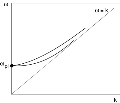
Figure 6: Plasmon spectrum in one loop.

The behavior of dispersive curves is schematically shown in Fig.6. At $k=0$, $\omega_{\bot}(0)=\omega_{\|}(0)=\omega_{pl}$. Then the two branches diverge:

$$\omega^{2}_{\bot}(k\ll gT)=\omega_{pl}^{2}+\frac{6}{5}k^{2}$$

$$\omega^{2}_{\|}(k\ll gT)=\omega_{pl}^{2}+\frac{3}{5}k^{2}$$ (5.7)

At $k\gg gT$ both branches tend to the vacuum dispersive law

$$\omega^{2}_{\bot}(k\gg gT)=k^{2}+\frac{3}{2}\omega_{pl}^{2}$$

$$\omega^{2}_{\|}(k\gg gT)=k^{2}\left[1+4\exp\left(-\frac{2k^{2}}{3\omega_{pl}^{2}}-2\right)\right]$$ (5.8)

We see that $\omega_{\|}(k)$ approaches the line $\omega=k$ exponentially fast.

The dispersive laws for quark collective excitations are obtained from a similar analysis of the quark Green’s function. At $T\neq 0$, the fermion polarization operator involves two tensor structures $\omega\gamma^{0}-{\bf k}{\bf\gamma}$ and $\omega\gamma^{0}+{\bf k}{\bf\gamma}$ which gives rise to two dispersive branches. We will call the branch corresponding to the Lorentz-invariant structure “transverse” and the branch corresponding to the structure $\omega\gamma^{0}+{\bf k}{\bf\gamma}$ — “longitudinal”. These terms may be misleading in the fermion case because, in contrast to the plasmons with photon or gluon quantum numbers, these branches are not associated with transverse and longitudinal field polarizations. Hence the quotation marks. But better names were not invented, and using the words “transverse” and “longitudinal” still makes a certain sense because the physical properties of “transverse” and “longitudinal” fermion branches are rather analogous to the physical properties of transverse and longitudinal gluon branches.

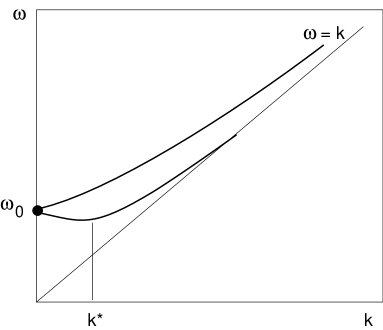
Figure 7: Plasmino spectrum in one loop.

The pattern of the quark spectrum is shown in Fig.7. It is similar to the gluon spectrum with one important distinction — at $k\sim 0$, $\omega_{\bot}(k)$ and $\omega_{\|}(k)$ involve linear terms of opposite sign:

$$\omega^{q}_{\bot}(k\ll gT)=\omega_{0}+\frac{k}{3}$$

$$\omega^{q}_{\|}(k\ll gT)=\omega_{0}-\frac{k}{3}$$ (5.9)

where $\omega_{0}$ is the plasmino frequency at zero momentum :

$$\omega_{0}^{2}=\frac{g^{2}T^{2}}{8}c_{F}$$ (5.10)

Thus, $\omega^{q}_{\|}(k)$ first goes down and reaches minimum at some $k^{*}$. The group velocity of the longitudinal plasmino at this point is zero.

5.2 Landau Damping.

The quoted one-loop results for the dispersive laws of transverse plasmons and plasminos are gauge-invariant and stable with respect to higher-order corrections. The latter is not true, however, for longitudinal excitation branches [38, 10]. We have seen that $\omega_{\|}^{1\ loop}(k)$ tends to the line $\omega=k$ exponentially fast at $k\gg gT$. This can be easily seen from the analysis of the dispersive equations for longitudinal branches which in the limit $k\gg gT$ have the form

$$\omega_{\|}+k\sim\frac{g^{2}T^{2}}{k}\ln\frac{k}{\omega_{\|}-k}$$ (5.11)

At $k\gg gT$, the solution exists when the logarithm is large and $\omega_{\|}-k$ is exponentially small. The logarithmic factor in Eq.(5.11) comes from the angular integral

$$\sim\int\frac{d\theta}{\omega-k\cos\theta}$$ (5.12)

which diverges at $\omega=k$. This collinear divergence appears due to masslessness of quarks and gluons in the loop depicted in Fig.1. But quarks and gluons in $QGP$ are not massless — their dispersive law acquires the gap $\sim gT$ due to temperature effects. An accurate calculation requires substituting in the loops the dressed propagators. As a result, the logarithmic divergence in the integral (5.12) is cut off and the logarithmic factor in Eq.(5.11) is modified:

$$\ln\frac{k}{\omega-k}\to\frac{1}{2}\ln\frac{k^{2}}{(\omega-k)^{2}+Cg^{2}T^{2}}$$ (5.13)

Dressing of propagators amounts to going beyond one-loop approximation. Strictly speaking, to be self-consistent one should also take into account one-loop thermal corrections to the vertices (this procedure is known as resummation of hard thermal loops [39]), but in this particular case these corrections do not play an important role. What is important is the cutoff of the logarithmic collinear singularity due to effective temperature-induced masses.

Substituting (5.13) in (5.11), we see that the new dispersive equation does not at all have solutions with real $\omega$ for large enough $k$. This fact can be given a natural physical explanation. When $k$ is small compared to $gT$, there is no logarithmic factor in the dispersive equation, the modification (5.13) is irrelevant, and the dispersive law of longitudinal modes does not deviate from the one-loop result. Then the logarithm appears, the modification (5.13) starts playing a role, and, at some $k^{**}\sim gT$, the longitudinal dispersive curve crosses the line $\omega=k$. At this point the longitudinal polarization operator acquires the imaginary part due to Landau damping.

In usual plasma, Landau damping is the process when propagating electromagnetic waves are “absorbed” by the electrons moving in plasma. In the language of quantum field theory, it is a $2\to 1$ process

$$\gamma^{*}+e\to e$$ (5.14)

In real time technique, that corresponds to a contribution to the imaginary part of the polarization operator so that both internal electron lines in the loop are placed on mass shell. At $T=0$ the standard Cutkovsky rules imply positive energies of all particles in the direct channel, and the imaginary part appears only due to the decay $\gamma^{*}\to e^{+}+e^{-}$. At $T\neq 0$, Cutkovsky rules are modified and both signs for energy are admissible. Physically, that corresponds to the presence of real particles in the heat bath so that the process (5.14) may go.

Also in $QGP$ imaginary parts of polarization operators may acquire contributions due to Landau damping. The corresponding processes are

$$g^{*}+g\to g,\ \ g^{*}+q\to q,\ \ q^{*}+g\to q,\ \ q^{*}+\bar{q}\to g,\ \ldots$$ (5.15)

where $g^{*},q^{*}$ are plasmon and plasmino collective excitations and $q,g$ are the excitations with characteristic momenta of order of temperature (in this kinematic region, the dispersive laws are roughly the same as for tree quarks and gluons and the star superscript is redundant).

The kinematic condition for the scattering processes (5.15) to go is that the frequency of collective excitations $g^{*}$ and $q^{*}$ would be less than their momentum. We have seen that the condition $\omega<k$ is realized indeed for longitudinal plasmon and plasmino excitations starting from some $k^{**}\sim gT$. At $k>k^{**}$, the Landau damping switches on and the dispersion law acquires an imaginary part. The imaginary part rapidly grows and very soon becomes of order of the real part. From there on it makes no sense to talk about propagating longitudinal modes anymore. The situation is the same as in usual plasma where longitudinal modes also become overdamped at large enough momenta and disappear from the physical spectrum [8].

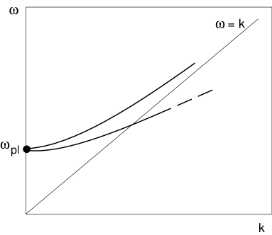
Figure 8: Plasmon spectrum.

The true pattern of plasmon collective modes is shown in Fig.8. A similar picture holds for plasminos.

5.3 Observability.

One-loop dispersive curves are gauge-invariant. However, the question whether these curves are physically observable is, again, highly non-trivial. It is easy to measure explicitly photon dispersive curves in usual plasma — to this end, one should study the propagating classical electromagnetic waves, measure the electric charge density (say, by laser beams) as a function of time and spatial coordinates and determine thereby the frequency and the wave vector of the wave.

But there is no such thing in Nature as classical gluon field due to confinement, and no classical device which would measure the color charge density exists. Even more obviously, quark fields (which have Grassmannian nature) cannot be treated classically. Hence, one cannot really measure the energy and momentum of propagating colored waves in a direct physical experiment.

What one can measure are correlators of colorless (in the first place , electromagnetic) currents. Modification of dispersive laws affects these correlators and that can be observed. However, a colorless current always couples to a pair of colored particles and, as a result, physical correlators involve some integrals of quark and gluon Green’s functions which are related to quark and gluon dispersive characteristics only in an indirect way. Also, thermal modification of vertices is as important here as modification of the Green’s functions.

However, there is one special point on the dispersive curves which can in principle be directly measured in experiment. This is the point on the longitudinal plasmino curve where its frequency acquires a minimal value and the group velocity turns to zero. Consider the problem of emission of relatively soft $e^{+}e^{-}$ or $\mu^{+}\mu^{-}$ pairs by $QGP$. In a “thermos bottle” experiment, one should make sure that the size of your thermos bottle is much less than the lepton mean free path. Otherwise, the leptons are thermalized and their spectrum is just Planckian. But in heavy ion collisions experiments, $QGP$ is produced in small volume, the condition $L_{\rm char}\ll L^{em}_{\rm free\ path}$ is satisfied, and the spectrum of emitted leptons (and photons) can provide a non-trivial information on dynamic characteristics of $QGP$.

The spectrum of soft dileptons was calculated in [40]. This is one of very few physical problems we know of where the hard thermal loop resummation technique [39] should be used (and was used) at full length. The spectrum feels the effects due to quark and gluon interactions in the region $E_{l^{+}l^{-}}\sim P_{l^{+}l^{-}}\sim gT$ — the spectrum at larger energies and momenta is the same as for the gas of free quarks. One particular source of soft dileptons is the process $q^{*}_{\bot}\to q^{*}_{\|}\ +\ l^{+}l^{-}$. The probability of this process has a “spike” for the momentum of $q_{\bot}^{*}$ and $q_{\|}^{*}$ coinciding with the momentum $k^{*}$ on the longitudinal plasmino dispersive curve with zero group velocity. There are just many plasminos at the vicinity of this point and the phase space factor provides a singularity at $E_{l^{+}l^{-}}=\omega_{\bot}(k^{*})-\omega_{\|}(k^{*})$ in the spectrum. Another spike comes from the process when a longitudinal plasmino with momentum $k^{*}$ annihilates with a longitudinal antiplasmino with the opposite momentum to produce a lepton pair with the energy $2\omega_{\|}(k^{*})$.

Unfortunately, in the soft region, the main contribution in the spectrum is due to cuts. In other words, the most relevant elementary kinetic processes are not $q^{*}\to q^{*}+l^{+}l^{-}$ or $q^{*}+\bar{q}^{*}\to l^{+}l^{-}$, but rather $q^{*}+g^{*}\to q^{*}+g^{*}+l^{+}l^{-}$ etc. The spikes actually have finite width due to collisional damping of collective excitations (the issue to be discussed in the next section), and one can hope to see only a tiny resonance on a huge background. Still, such a resonance in the spectrum is an observable effect.

6 Damping Mayhem and Transport Paradise.

6.1 Direct decay.

In the previous section, we discussed the Landau damping contribution to the imaginary parts of polarization operators and, correspondingly, to imaginary parts of dispersion laws. It comes from the kinematic region $\omega<k$ and is physically related to absorbtion of ingoing excitations by thermal quanta like in (5.15). However, we did not say a word about the contribution of direct decay processes $g^{*}\to q+\bar{q}$ etc. in the timelike kinematic region $\omega>k$.

That was with a good reason. On the one-loop level, the contribution of decay processes in imaginary parts is nonzero and is of order $\sim g^{2}T$. Unfortunately, it depends on the gauge and, in some gauges, has even the wrong sign corresponding not to damping of excitations but to instabilities [41]. The point is that such one-loop calculation is unstable with respect to higher-order corrections. It is very clear physically — quarks and gluons in $QGP$ cannot be treated as massless but acquire dynamical masses due to thermal effects. And the decay of a plasmon or plasmino into two other collective excitations is not kinematically allowed. The only exception is the process $g^{*}\to q^{*}+\bar{q}^{*}$ which in principle may go if [10]

$$N_{f}>9c_{F}-c_{V}=6$$ (6.1)

But there are at most three light flavors in real $QGP$ and decay processes can be safely forgotten.

6.2 Collisional damping.

Still, damping is there even in the timelike region $\omega>k$ due to collisions $g^{*}+q^{*}\to g^{*}+q^{*}$, $q^{*}+\bar{q}^{*}\to g^{*}+g^{*}$ etc. This is also the main source of damping of transverse electromagnetic waves in usual plasma [8]. A rough estimate for collisional damping in $QGP$ can be done very simply.

The meaning of damping is the inverse lifetime of excitations. We have

$$\zeta\sim(\tau_{life})^{-1}\sim n\sigma^{tot}$$ (6.2)

where $n\sim T^{3}$ is the density of the medium and $\sigma^{tot}$ for excitations which carry (color) charge has a Coulomb form

$$\sigma^{tot}\sim g^{4}\int\frac{dp_{\bot}^{2}}{p_{\bot}^{4}}\sim\frac{g^{2}}{T^{2}}$$ (6.3)

We took into account the fact that the power infrared divergence for the integral of Coulomb cross section is effectively cut off at $p_{\bot}\sim gT$ due to Debye screening . As a result, we obtain the estimate

$$\zeta^{q,g}\sim g^{2}T$$ (6.4)

Note that this value for the damping is unusually large. It is much larger than, say, the damping of photons in ultrarelativistic $e^{+}e^{-}$ – plasma. The latter can also be estimated from the formula (6.2), but $\sigma^{tot}$ is now not the Coulomb, but the Compton cross section. The integral has now the form $\int_{eT}dp_{\bot}^{2}/p_{\bot}^{2}\sim\ln(1/e)$ and the estimate is

$$\zeta^{\gamma}\sim e^{4}T\ln(1/e)\ll e^{2}T$$ (6.5)

The question arises whether the new anomalously large scale $\sim g^{2}T$ has a  physical  relevance . We will return to discussion of this point a bit later.

Figure 9:

An accurate calculation of the damping of fast moving ($k\gg gT$) quark and gluon excitations in $QGP$ has been done in [10, 11] (see also [42]). Consider the graph in Fig.9 for the quark polarization operator where the lines with blobs stand for quark and gluon propagator dressed by thermal loops. The imaginary part of the whole loop in Fig.9 depends on the imaginary parts of internal propagators. The imaginary part of the gluon propagator due to Landau damping turns out to be of paramount importance. Physically, this contribution just corresponds to the scattering processes $g^{*}+q^{*}\to g^{*}+q^{*}$ and $g^{*}+g^{*}\to g^{*}+g^{*}$ as can be easily inferred if spelling out the exact gluon propagator as in Fig.10 (there is also a similar graph with internal gluon loop).

Figure 10: A graph contributing to ${\rm Im}\ \Sigma(k)$. Crossed lines are put on mass shell. One of the quarks in the internal loop has a negative energy.

Dressing the quark propagator (indicated by the blob in Fig.10) is important. If not taking it into account, the imaginary part of the propagator is $\delta$ – function and the result for ${\rm Im}\ \Sigma(k)$ has the form

$${\rm Im}\ \Sigma(k)=-\frac{3}{32\pi}\omega_{pl}^{2}g^{2}c_{F}T\gamma^{0}\int dp_{0}\delta(p_{0}-p\cos\theta)\int_{-1}^{1}d\cos\theta\int\frac{dp^{2}}{p^{4}+\frac{9}{16}\omega_{pl}^{4}\frac{p_{0}^{2}}{p^{2}}}$$ (6.6)

The integral has a power infrared behavior at $p\gg gT$, but this divergence is cut off due to Landau damping effects [the second term in the denominator in the RHS of Eq.(6.6)]. Still, the integral in (6.6) diverges logarithmically at $p\ll gT$ and the result for the damping inferred from Eq.(6.6) is infinite.

The crucial observation is that the dressed quark propagator does not have singularities on the real $p_{0}$ axis. A self-consistent account of the collisional damping for the quark Green’s function moves its singularities in the complex plane. As a result, $\delta$ – function in the integrand is replaced by a smooth distribution with the width of order $\zeta\sim g^{2}T$. This smoothing cuts off the logarithmic singularity in (6.6) at $p\sim g^{2}T$. The other source for the cutoff could be provided by magnetic screening effects , but the latter is an essentially non-abelian phenomenon whereas the cutoff due to smearing out the $\delta$ – function is a universal effect which occurs also in an abelian theory.

To find the dispersion law, one should add Eq.(6.6) to the one-loop result for $\Sigma(k)$ and solve the dispersive equation. The solution is complex $\omega^{pole}(k)=\omega^{1\ loop}(k)-i\zeta(k)$ and the final result for $\zeta(k\gg gT)$ is very simple.

$$\zeta^{q}=\alpha_{s}c_{F}T\ln(C^{q}/g)$$

$$\zeta^{g}=\alpha_{s}c_{V}T\ln(C^{g}/g)$$ (6.7)

Only the coefficient of logarithm can be calculated. The constants $C^{q},\ C^{g}$ under the logarithm cannot determined. Actually, we will see shortly that these constants are gauge–dependent and cannot be defined in a reasonable way.

Figure 11: Polarization operator of soft plasmino.

Damping of excitations in another kinematic region ${\bf k}=0$ (“standing” plasmons and plasminos) was studied in [39]. Here the vertex corrections are as important as corrections to the propagators, however an accurate analysis of [39] shows that it suffices to take into account only one (hard thermal) loop corrections both in polarization operators and vertices. Consider for definiteness the damping of standing plasminos. The graphs contributing to the soft plasmino polarization operator are shown in Fig.11. Using Keldysh technique one can derive in the limit of soft external momentum

$$\Sigma^{R}(k)=-2ig^{2}\int\frac{d^{4}q}{2\pi^{4}}\frac{T}{q}_{0}{\rm Im}\ D_{\mu\nu}^{R}(q)\left[\frac{1}{2}\Gamma^{R}_{\mu\nu}(k;q)+\right.$$

$$\left.\Gamma^{R}_{\mu}(k,q+k;q)G^{R}(q+k)\Gamma_{\nu}^{R}(q+k,k;-q)\right]$$ (6.8)

($G^{R}$ and $D^{R}$ are the retarded Green’s functions and $\Gamma^{R}$ are the retarded vertices). Subsituting here transverse and longitudinal parts of the gluon Green’s function and one-loop vertices $\Gamma_{\mu\nu}$ and $\Gamma_{\mu}$, calculating the integral (which in this case can be done only numerically), and solving the dispersive equation, one arrives at the result

$$\zeta^{q}(k=0)=1.43c_{F}\frac{g^{2}T}{4\pi}$$ (6.9)

However, the gluon Green’s function involves also a gauge-dependent part

$$D_{\mu\nu}^{R(\alpha)}(q)=(\alpha-1)\frac{q_{\mu}q_{\nu}}{[(q_{0}+i\epsilon)^{2}-q^{2}]}$$ (6.10)

where $\alpha$ is a gauge parameter and an infinitesimal $i\epsilon$ is introduced to provide for the right analytical properties. At first sight, this gauge-dependent piece should not affect the position of the pole. Really, one can use the Ward identities (which hold also at finite temperature for retarded propagators and vertices [46, 11]) to derive

$$\Sigma^{R(\alpha)}(k)=-ig^{2}Tc_{F}(\alpha-1)[G^{R}(k)]^{-1}\int\frac{d^{4}q}{2\pi^{4}}\frac{1}{q}_{0}\left\{\frac{1}{[(q_{0}+i\epsilon)^{2}-q^{2}]}-\frac{1}{[(q_{0}-i\epsilon)^{2}-q^{2}]}\right\}$$

$$\left[G^{R}(k+q)-G^{R}(k)\right][G^{R}(k)]^{-1}$$ (6.11)

We see the presence of factors $[G^{R}(k)]^{-1}$ both on the right and on the left. $G^{R}(k)$ is singular at the pole and $[G^{R}(k)]^{-1}$ is zero. One might infer from this that a gauge-dependent contribution to $\Sigma^{R}({\rm pole})$ and hence to the corresponding solution of the dispersive equation determining the pole position is also zero.

However, this is wrong [47, 12]. The point is that the integral in (6.2) involves a severe power infrared divergence and is infinite at the pole. We have a thereby $0\times\infty$ uncertainty. This uncertainty can be resolved by choosing $k$ not exactly at the pole but slightly off mass shell. Then $[G^{R}(k)]^{-1}$ is not exactly zero and also the divergence in the integral is cut off by an off-mass-shellness. When the distance from the mass shell is small, the final result for $\Sigma^{R(\alpha)}(k\to{\rm pole})$ does not depent on this distance and is just finite. In the soft momenta region

$$\Sigma^{R(\alpha)}_{\rm soft}(k)=-\frac{i(\alpha-1)g^{2}Tc_{F}}{4\pi}\gamma^{0}$$ (6.12)

This brings about a gauge-dependent part $\sim g^{2}T$ in the damping of soft plasminos. A similar analysis with the same conslusion can be carried out for plasmons.

The same gauge-dependence shows up in the damping of energetic plasmons and plasminos, but in the latter case, this gauge-dependence is parametrically overwhelmed by the leading gauge-independent contribution (6.2) involving the factor $\ln(1/g)$.

6.3 Observability.

The observed gauge-dependence of the damping obviously indicates that it is not a physical quantity. This is definitely true at least for soft plasmons and plasminos where the gauge-dependent part and the gauge-independent part (6.9) are of the same order $\sim g^{2}T$.

Indeed, it is not possible to contemplate a physical experiment where this quantity could be measured. That should be confronted with the case of abelian plasma where damping of electromagnetic waves is a perfectly physical quantity and can be directly observed by measuring the attenuation of the amplitude of a classical wave with time. But as we already noted, no classical gluon or quark waves exist. This observation refers also for damping of electron and positron collective excitations in the ultrarelativistic abelian plasma. It also has an anomalously large scale $\sim e^{2}T$ (with the extra logarithmic factor  $\ln(1/e)$ for $k\gg eT$) and it also cannot be directly measured.

One could try to observe the effects due to damping in gauge-invariant quantites like the polarization operator of electromagnetic currents. An accurate analysis which goes beyond the conventional hard thermal loop resummation technique and effectively resums a set of ladder graphs shows, however, that a self-consistent account of the corrections due to damping in the quark Green’s functions and in the vertices results in the exact cancellation of the anomalously large scale $\sim g^{2}T$ in the final answer [11]. (for a similar analysis with a similar conclusion in scalar QED see [48]).

However, there is a physical problem where the scale $\sim g^{2}T$ can in principle show up. This is the already discussed problem of lepton pair production in $QGP$. We have seen that the spectrum of leptons pairs invoves spikes associated with a special point with zero group velocity on the longitudinal plasmino dispersive curve. Going beyond the hard thermal loop aproximation and taking into account the effects due to collisional damping in the Green’s functions and in the vertices would bring about a finite width for these spikes of order $g^{2}T$ and there is a principle possibility to measure this width. This problem has not been studied, and it is not clear by now whether the width of the spike can by calculated analytically and whether one can single out this spike out of the background.

What one can say quite definitely is that this width crucially depends on modification of vertices due to collisional effects and has nothing to do with the (gauge-dependent) position of the pole (or whatever the real singularity is [43, 12, 44]) of the quark and gluon Green’s function.

Thus, we are convinced that the latter is not a physical quantity probably even for energetic plasmons in spite of the fact that the leading contribution (6.2) is gauge-independent there. We just do not know how on Earth this quantity could be measured.

6.4 Transport Phenomena.

There is a lot of kinetic phenomena in $QGP$ which are physical and measurable. Indeed, nothing in principle prevents measuring the electric resistance of a vessel with $QGP$ or studying the flow of $QGP$ through narrow tubes. They do not depend, however, on the anomalous damping scale $g^{2}T$, but rather on a much smaller scale

$$(\tau_{char})^{-1}\sim g^{4}T\ln(1/g)$$ (6.13)

This scale already appeared in (6.5) determining the damping of electromagnetic waves in $e^{+}e^{-}$ – plasma. And it is also the scale which determines the mentioned physical effects of viscousity and electric conductivity, and many others — heat conductivity, energy losses of a heavy particle moving through plasma, etc.

The appearance of the scale $g^{4}T\ln(1/g)$ has a clear physical origin. All the mentioned effects are inherently related to the rate of relaxation of the system to thermal equilibrium. The latter can be estimated as

$$(\tau_{rel})^{-1}\sim n\sigma^{trans}$$ (6.14)

It looks the same as the estimate for lifetime (6.2) but with an essential difference — in contrast to (6.2), the estimate (6.14) involves the transport rather than the total cross section. The transport cross–section is defined as

$$\sigma^{trans}=\int d\sigma(1-\cos\theta)$$ (6.15)

where $\theta$ is the scattering angle. The factor $(1-\cos\theta)$ takes care of the fact that small–angle scattering though contributes to the total cross section, does not essentially affect the distribution functions $n_{g}({\bf p})$, $n_{q}({\bf p})$ and is not effective in relaxation processes. For the Coulomb scattering in ultrarelativistic plasma, the transport cross section is

$$\sigma^{trans}\sim g^{4}\int_{(gT)^{2}}\frac{dp_{\bot}^{2}}{p_{\bot}^{4}}\frac{p_{\bot}^{2}}{T^{2}}\sim\frac{g^{4}}{T^{2}}\ln\frac{1}{g}$$ (6.16)

Multiplying it by $n\sim T^{3}$ and substituting it in (6.14), the estimate (6.13) is reproduced.

Viscousity and all other similar quantities can be calculated analytically in the leading order (probably, magnetic infrared divergences prevent an analytic evaluation of these quantities in next orders in $g$, but this question is not yet well studied). It is interesting that Feynman diagram technique proves to be technically unconvenient here , and the good old Boltzmann kinetic equation is the tool people usually use (see e.g. [49]).

Let us make two illustrative estimates which make clear how the relaxation scale (6.13) depending on the transport cross–section (6.16) arises.

First, let us estimate the electric conductivity of $QGP$ (it is the quite conventional conductivity, not the “color conductivity” which is sometimes discussed in the literature, depends on the anomalous damping scale $g^{2}T$, and is not a physically observable quantity — we do not have batteries with color charge at our disposal). Suppose at $t=0$ the system was at thermal equilibrium so that the quark distribution functions are $n_{0}({\bf p},{\bf x},t=0)=n_{F}(|{\bf p}|)$. When we switch on the electric field, the distribution function starts to evolve according to the kinetic equation

$$\frac{\partial n({\bf p},{\bf x},t)}{\partial t}+{\bf v}\frac{\partial n({\bf p},{\bf x},t)}{\partial{\bf x}}=e{\bf E}\frac{\partial n({\bf p},{\bf x},t)}{\partial{\bf p}}+\ldots$$ (6.17)

Dots in RHS of Eq.(6.17) stand for the collision term which becomes relevant at $t\sim x\sim\tau_{\rm rel}\sim\tau_{\rm free\ path}\sim[g^{4}T\ln(1/g)]^{-1}$. Thus, the electric field brings about distortions of the distribution function which grow up to the characteristic value

$$\delta n\sim e{\bf E}\frac{{\bf v}}{T}n_{0}\tau_{\rm free\ path}\sim\frac{e{\bf E}{\bf v}T}{g^{4}\ln(1/g)}$$

At this point, collisional effects stop the growth (a particle drifting in external electric field collides with a particle in the medium, forgets what happened before, and starts drifting anew). The density of electric current in the medium is

$${\bf j}=e\int{\bf v}\delta n\ d^{3}p\sim{\bf E}\frac{e^{2}T}{g^{4}\ln(1/g)}$$ (6.18)

The coefficient between ${\bf j}$ and ${\bf E}$ gives the conductivity.

Let us estimate now the energy losses of a heavy energetic quark in $QGP$. Of course, free quarks do not exist, but a physical experimental setup would be sending into the bottle with $QGP$ a heavy meson ${Q}\bar{q}$ with open beauty or top. In $QGP$, the meson dissociates, and a naked heavy quark propagates losing its energy due to interaction with the medium. It goes out then on the other side of the bottle dressed again with light quarks, but not necessarily in the same way as before. When $M_{Q}\gg\Lambda_{QCD}$, this dressing does not essentially affect its energy. A heavy particle containing $Q$ can be detected and its energy can be measured.

Suppose a heavy quark is ultrarelativistic, but its energy is not high enough for the Cerenkov radiation processes to be important. Then the energy would be lost mainly due to individual incoherent scatterings. The mean energy loss in each scattering is $\Delta E\sim T$ ($T$ — is a characteristic energy of the particles in heat bath on which our heavy quark scatters). The mean time interval between scatterings is $\tau_{\rm free\ path}\sim[g^{4}T\ln(1/g)]^{-1}$. We obtain

$$-\frac{dE}{dx}\sim\frac{\Delta E}{\tau_{\rm free\ path}}=C\alpha_{s}^{2}T^{2}\ln(1/g)$$ (6.19)

This estimate turns out to be correct up to the argument of the logarithm which in reality is energy–dependent [50]. The numerical coefficient $C=4\pi c_{F}/3$ was determined by Bjorken [51]

7 Acknowledgements.

I am indebted to J.P. Blaizot, S. Peigne, E. Pilon, A. Rebhan, and E. Shuryak for useful discussions, remarks and references. This work has been done under the partial support of INTAS Grants CRNS–CT93–0023, 93–283, and 94–2851.

References

- [1] J.W. Harris and B. Muller, Preprint DUKE-TH-96-105, hep-ph/9602235.
- [2] J.D. Bjorken, Acta Physica Polonica B23 (1992) 561; J.-P. Blaizot and A. Krzywicki, Phys. Rev. D46 (1992) 246; J.D. Bjorken, Talk on the Workshop Continuous Advances in QCD, Minneapolis, 1994 (World Scientific, Singapore, 1994).
- [3] A.V. Smilga, Thermal Phase Transition in , Lecture at the International School “Enrico Fermi” (Varenna, July 1995), hep-ph/9508305.
- [4] T. Matsubara, Progr. Theor. Phys. 14 (1955) 351.
- [5] L.S. Brown, Quantum Field Theory, (Cambridge University Press, Cambridge, England, 1992).
- [6] P.M. Bakshi and K.T. Mahanthappa, J. Math. Phys. 4 (1963) 1; 12.
- [7] L.V. Keldysh, Zh.E.T.F. 47 (1964) 1515.
- [8] E.M. Lifshitz and L.P. Pitaevsky, Physical Kinetics, Pergamon Press, 1981.
- [9] N.P. Landsman and Ch.G. van Weert, Phys. Rep., 145 (1987) 142.
- [10] V.V. Lebedev and A.V. Smilga, Ann. Phys. 202 (1990) 229.
- [11] V.V. Lebedev and A.V. Smilga, Phys. Lett. 253B (1991) 231; Physica A181 (1992) 187.
- [12] A.V. Smilga, Physics of Atomic Nuclei 57(1994) 519.
- [13] L. Dolan and R. Jackiw, Phys. Rev. D9 (1974) 3320.
- [14] A.M. Polyakov, Gauge Fields and Strings, Harwood Academic Publishers, Chur, Switzerland, 1987.
- [15] S. Dalley and I.R. Klebanov, Phys. Rev. D47 (1993) 3517; G. Bhanot, K. Demeterfi and I.R. Klebanov, Nucl. Phys. B418 (1994) 15.
- [16] R. Hagedorn, Nuovo Cimento Suppl. 3 (1965) 147; R. Hagedorn and J. Ranft, ibid 6 (1968) 169.
- [17] E. Shuryak, J.E.T.P. 47 (1978) 212; Phys. Repts. 61 (1980) 71.
- [18] A.M. Polyakov, Phys. Lett. 72B (1978) 477 ; L. Susskind, Phys. Rev. D20 (1979) 2610.
- [19] L. McLerran and B. Svetitsky, Phys. Rev. D24 (1981) 450; J. Kuti, J. Polonyj and K. Szlachanyi, Phys. Lett 66 (1991) 998.
- [20] A.D. Linde, Phys. Lett. B96 (1980) 289.
- [21] S. Nadkarni, Phys. Rev. D33 (1986) 3738.
- [22] P. Arnold and C.G. Yaffe, Phys. Rev. D52 (1995) 7208.
- [23] S. Peigne and S.M.H. Wong, Phys. Lett. B346 (1995) 322.
- [24] T. Toimela, Z.Phys. C27 (1985) 289.
- [25] A. Rebhan, Nucl. Phys. B430 (1994) 319.
- [26] A.V. Smilga, Annals of Physics, 234 (1994) 1.
- [27] J.I. Kapusta, Nucl. Phys. B148 (1979) 461; Finite Temperature Field Theory (Cambridge University Press, Cambridge, England, 1989).
- [28] T. Toimela, Phys. Lett. 124B (1983) 407.
- [29] P. Arnold and C. Zhai, Phys. Rev. D50 (1994) 7603; D51 (1995) 1906.
- [30] B. Kastening and C. Zhai, Phys. Rev. D52 (1995) 7232.
- [31] E. Braaten and A. Nieto, Phys. Rev. D53 (1996) 3421.
- [32] E. Shuryak, Phys. Rev. Lett. 68 (1992) 3270.
- [33] M. B. Voloshin, Int. J. Mod. Phys. A10 (1995) 2865.
- [34] J.P. Blaizot and E. Iancu, Nucl. Phys. B434 (1995) 662.
- [35] V.V. Lebedev, A.V. Smilga, Nucl. Phys. B318 (1989) 669.
- [36] O.K. Kalashnikov and V.V. Klimov, Yadernaja Fizika 31 (1980) 135; V.V. Klimov, Zh.E.T.F. 82 (1982) 336.
- [37] H. A. Weldon, Phys. Rev. D26 (1982) 1384; 2789.
- [38] V.P. Silin and V.N. Ursov, Lebedev Institute Reports (Sov. Phys.) #5 (1988) 33.
- [39] E. Braaten and R.D. Pisarski, Nucl. Phys. B337 (1990) 569; Phys. Rev. D45 (1992) 1827.
- [40] E. Braaten, R.D. Pisarski and T.C. Yuan, Phys. Rev. Lett. 64 (1990) 2242.
- [41] K. Kajantie and J. Kapusta, Ann. Phys. 160 (1985) 477 ; U. Heinz, K. Kajantie and T. Toimela, Phys. Lett. 183B (1987) 96; H. Th. Elze et al, Z. Phys. C37 (1988) 305; T.H. Hanson and I. Zahed, Nucl. Phys. B292 (1987) 725.
- [42] T. Altherr, Phys. Rev. D47 (1993) 482.
- [43] R. Baier, H. Nakkagawa and A. Niegawa, Can J. Phys. 71 (1993) 205.
- [44] E. Pilon, Private communication.
- [45] J.P. Blaizot and E. Iancu, Preprint Saclay – T95/146; hep-ph/9601205.
- [46] J. Frenkel and J.C. Taylor, Nucl. Phys. B334 (1990) 199; J.C. Taylor and S.M.H. Wong, Nucl. Phys. B346 (1990) 115.
- [47] R. Baier, G. Kunstatter and D. Schiff, Phys. Rev. Lett. 64 (1990) 2992; Nucl. Phys. B355 (1991) 1.
- [48] U. Kramer, H. Schulz and A. Rebhan, Ann. Phys. 238 (1995) 286.
- [49] G.Baym et al, Phys. Rev. Lett. 64 (1990) 1867.
- [50] M.H. Thoma and M. Gyulassy, Nucl. Phys. B351 (1991) 491; E. Braaten and M.H. Thoma, Phys. Rev. D44 (1991) R2625.
- [51] J.D. Bjorken, Fermilab Report # PUB–82/59–THY (unpublished).