Abstract

We present the complete next-to-leading order short-distance QCD corrections to the effective $\mathrm{|\Delta S|\!=\!2}$-hamiltonian in the Standard Model. The calculation of the coefficient $\eta_{3}$ is described in great detail. It involves the two-loop mixing of bilocal structures composed of two $\mathrm{|\Delta S|\!=\!1}$ operators into $\mathrm{|\Delta S|\!=\!2}$ operators. The next-to-leading order corrections enhance $\eta_{3}$ by 27% to

$$\eta_{3}=0.47\raisebox{-2.15277pt}{\shortstack[l]{$\scriptstyle+0.03$\\ $\scriptstyle-0.04$}}$$

thereby affecting the phenomenology of $\epsilon_{K}$ sizeably. $\eta_{3}$ depends on the physical input parameters $m_{t}$, $m_{c}$ and $\Lambda_{\overline{\mathrm{MS}}}$ only weakly. The quoted error stems from renormalization scale dependences, which have reduced compared to the old leading log result. The known calculation of $\eta_{1}$ and $\eta_{2}$ is repeated in order to compare the structure of the three QCD coefficients. We further discuss some field theoretical aspects of the calculation such as the renormalization group equation for Green’s functions with two operator insertions and the renormalization scheme dependence caused by the presence of evanescent operators.

1 Introduction

$\mathrm{|\Delta S|\!=\!2}$ transitions induce the mixing between the neutral Kaon states $\mathrm{K^{0}}$ and $\mathrm{\overline{K^{0}}}$. The investigation of $\mathrm{K^{0}\!-\!\overline{K^{0}}}\,$-mixing  has revealed a lot about the short distance structure of nature: In 1970 Glashow, Iliopoulos and Maiani (GIM) postulated the existence of the charm quark [1] from the suppression of this and other flavour-changing neutral current (FCNC) processes. Then Gaillard and Lee estimated the mass of the charm quark from the measured value of the $\mathrm{K_{L}\!-\!K_{S}}\,$-mass difference  [2]. Further the violation of the CP symmetry in nature has been first observed in $\mathrm{K^{0}\!-\!\overline{K^{0}}}\,$-mixing  [3] in 1964, long before the Standard Model of elementary particles has been constructed. The quantity $\epsilon_{K}$ characterizing this indirect CP-violation is up to now the only unambiguously determined measure of CP-violation in nature. Well before the discovery of the $\tau$ lepton Kobayashi and Maskawa [4] realized that the explanation of CP-violation within the Standard Model requires a third fermion family. In the subsequent decades the analysis of $\epsilon_{K}$ has clearly been indispensable in the determination of the elements of the Cabibbo-Kobayashi-Maskawa (CKM) matrix. Here the CKM phase $\delta$, which is the only source of CP-violation in the Standard Model, is derived as a function of four key parameters: the magnitudes of the CKM elements $V_{cb}$ and $V_{ub}$, the non-perturbative QCD parameter $B_{K}$ and the top quark mass $m_{t}$. $\epsilon_{K}$ depends on $m_{t}$, because $\mathrm{K^{0}\!-\!\overline{K^{0}}}\,$-mixing is a loop process with top quarks in the intermediate state. As a special feature one cannot find a solution for $\delta$ from the measured value of $\epsilon_{K}$ for too low values of the four key quantities. This has allowed to derive lower bounds on $m_{t}$ in the time before the top discovery. Yet now in the top era one can use the measured value for $m_{t}$ to constrain the allowed region for the CKM parameters [6]. But also the accuracy of the other three parameters in the game has made significant progress in the last few years. To keep up with this progress the theorist’s tools to predict the strength of the $\mathrm{|\Delta S|\!=\!2}$ transitions must be sharpened as well, as we will show in the following.

To be specific, let us look at the $\mathrm{|\Delta S|\!=\!2}$-hamiltonian:

$$H^{\mathrm{|\Delta S|\!=\!2}} = \frac{G_{F}^{2}}{16\pi^{2}}M_{W}^{2}\,\left[\,\lambda_{c}^{2}\,\eta_{1}\,S(\frac{m_{c}^{2}}{M_{W}^{2}})\>+\>\lambda_{t}^{2}\,\eta_{2}\,S(\frac{m_{t}^{2}}{M_{W}^{2}})\right.$$ (1)

$$\phantom{\frac{G_{F}^{2}}{16\pi^{2}}M_{W}^{2}\,}\left.+\,2\,\lambda_{c}\,\lambda_{t}\,\eta_{3}\,S(\frac{m_{c}^{2}}{M_{W}^{2}},\frac{m_{t}^{2}}{M_{W}^{2}})\,\right]b(\mu)\tilde{Q}_{S2}(\mu)\>+\>\mathrm{h.c.}$$

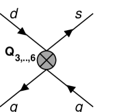
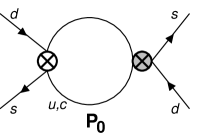
Here $G_{F}$ is the Fermi constant, $\lambda_{j}=V_{jd}V_{js}^{*}$ comprises the CKM-factors, and $\tilde{Q}_{S2}$ is the local four quark operator (see Fig. 2)

$$\tilde{Q}_{S2} = (\overline{s}_{j}\gamma_{\mu}(1-\gamma_{5})d_{j})(\overline{s}_{k}\gamma^{\mu}(1-\gamma_{5})d_{k})\;=\;(\overline{s}d)_{V-A}(\overline{s}d)_{V-A}$$ (2)

with $j$ and $k$ being colour indices. The Inami-Lim functions $S(x)$ and $S(x,y)$ [5] depend on the masses of the charm- and top quark and describe the $\mathrm{|\Delta S|\!=\!2}$ transition amplitude in the absence of strong interactions. They are obtained by calculating the lowest order box diagrams depicted in Fig. 2.

 

Figure 1: The diagram for the matrix element of $\tilde{Q}_{S2}$ to order $\alpha_{s}^{0}$. The cross denotes the insertion of the effective $\mathrm{\Delta S}=-2$ operator $\tilde{Q}_{S2}$.

Figure 2: The lowest order box diagrams mediating a $\mathrm{|\Delta S|\!=\!2}$ transition. The zigzag lines stand for W-bosons or fictitious Higgs particles. The diagrams rotated by 90^∘ must also be considered.

 

We will be interested in the short distance QCD corrections comprised in the coefficients $\eta_{1}$, $\eta_{2}$ and $\eta_{3}$ with a common factor $b(\mu)$ split off. They describe the effect of dressing the lowest order diagram in Fig. 2 with gluons in all possible ways. The $\eta_{i}$’s are functions of the charm and top quark masses and of the QCD scale parameter $\Lambda_{\mathrm{QCD}}$. Further they depend on various renormalization scales. This dependence, however, is artificial, as it originates from the truncation of the perturbation series, and diminishes order-by-order in $\alpha_{s}$.

The hadronic matrix element of $\tilde{Q}_{S2}$ between the neutral Kaon states is parametrized as

$$\langle\overline{K^{0}}\mid\tilde{Q}_{S2}(\mu)\mid{K^{0}}\rangle = \frac{8}{3}\frac{B_{K}}{b(\mu)}f_{K}^{2}m_{K}^{2}.$$ (3)

Here $m_{K}$ and $f_{K}$ are mass and decay constant of the neutral K meson and $\mu$ is the renormalization scale at which the short distance calculation of (1) is matched with the non-perturbative evaluation of (3). $B_{K}$ in (3) is defined in a renormalization group (RG) invariant way, because the $\mu$-dependent terms cancel when the physical matrix element $\langle\overline{K^{0}}\mid H^{\mathrm{|\Delta S|\!=\!2}}\mid{K^{0}}\rangle$ is expressed in terms of $B_{K}$.

The first determination of (1) in the free quark model (i.e. with $\eta_{i}\cdot b(\mu)=1$) is due to Vaĭnsteĭn and Khriplovich [7] and Gaillard and Lee [2]. Then the QCD factor $\eta_{1}$, which is only sensitive to the first two quark families, has been calculated in the leading-logarithmic approximation by Vaĭnsteĭn, Zakharov, Novikov and Shifman [8]. They have explicitly extracted the coefficient of the leading logarithm $\alpha_{s}\ln(m_{c}^{2}/M_{W}^{2})$ from the diagrams depicted in Fig. 3 and summed this logarithm to all orders in perturbation theory with the help of the RG equation. In the same way the coefficient $\eta_{2}$ has been obtained by Vysotskiĭ [9] for the case of a light top quark. Then Gilman and Wise [10] have introduced a more efficient method to achieve the leading log summation. Following Witten [11] they have applied Wilson’s operator product expansion [12] consequently to the $\mathrm{|\Delta S|\!=\!1}$-substructure and could reproduce the results of [8, 9] for $\eta_{1}$ and $\eta_{2}$. Further they have correctly determined $\eta_{3}$, which involves a larger operator basis than $\eta_{1}$ and $\eta_{2}$ due to the presence of penguin operators [13]. It is difficult, if not impossible, to achieve this calculation with the older methods of [8, 9]. Further the leading order (LO) calculation of [10] has only required one-loop calculations to obtain the leading logarithms of the diagrams in Fig. 3. The results of [10] have later been extended to the case of a heavy top quark by Flynn and by Datta, Fröhlich and Paschos [14].

Yet LO results suffer from certain systematic drawbacks and a precision calculation must include the next-to-leading order (NLO) terms. We sketch the reasons here:

1. The fundamental QCD scale parameter $\Lambda_{\overline{\mathrm{MS}}}$ is not well-defined in the LO.

2. The quark mass dependence of the $\eta_{i}$’s is not correctly reproduced by the LO expressions. Especially the $m_{t}$-dependent terms in $\eta_{3}\cdot S(x_{c},x_{t})$ belong to the NLO.

3. Similarly the question of the definition of the quark masses (i.e. the renormalization scheme and scale) to be used in (1) is a next-to-leading order issue: Hence one has to go to the NLO to know how to use $m_{t}$ as determined at Fermilab in low-energy hamiltonians like (1).

4. The LO results for $\eta_{1}$ and $\eta_{3}$ show a large dependence on the renormalization scales, at which one integrates out heavy particles. In the NLO these uncertainties are reduced considerably.

5. One must go to the NLO to judge whether perturbation theory works, i.e. whether the radiative corrections are small. After all the corrections can be sizeable.

 

Figure 3: The classes of diagrams constituting the $O(\alpha_{s})$-contribution to $\mathrm{|\Delta S|\!=\!2}$ transitions in the SM; the remaining diagrams are obtained by left-right and up-down reflections. The curly lines denote gluons. Also QCD counterterm diagrams have to be included. Diagram $\mathsf{F_{8}}$ equals 0 for zero external momenta.

 

The first step of the extension of (1) beyond the leading order has been done by Buras, Jamin and Weisz, who have derived the NLO expression for $\eta_{2}$ [15]. Then we have calculated $\eta_{1}$ in the NLO [16], and the present work is devoted to present the details of our NLO calculation of $\eta_{3}$. For completeness we will also list the results of [15, 16] for $\eta_{1}$ and $\eta_{2}$ and illustrate the different structure of $\eta_{1}$, $\eta_{2}$ and $\eta_{3}$. The numerical results and the phenomenological implications of our findings on the analysis of $\epsilon_{K}$ and the $\mathrm{K_{L}\!-\!K_{S}}\,$-mass difference  have already been given in [6] (for an update see [17]). We assume that the reader is familiar with the general concepts of Wilson’s operator product expansion, the renormalization group and operator mixing. A detailed description of these tools in the context of $\mathrm{K^{0}\!-\!\overline{K^{0}}}\,$-mixing  can be found in [18, 19].

The paper is organized as follows: In sect. 2 we first set up our notation and then discuss the $\mathrm{|\Delta S|\!=\!2}$ transition in the Standard Model (SM). We identify the large logarithms in the transition amplitude to orders $\alpha_{s}^{0}$ and $\alpha_{s}^{1}$ and compare their numerical sizes. Sect. 3 is devoted to the effective description of the $\mathrm{|\Delta S|\!=\!2}$ transition between the scales $\mu_{tW}=O(m_{t},M_{W})$, at which the top quark and the W-boson are integrated out, and $\mu_{c}=O(m_{c})$, at which the charm quark is removed as a dynamic degree of freedom. Here we construct the operator basis used in the effective lagrangian. We then match the SM amplitude to the effective matrix elements at the initial scale $\mu_{tW}$ and determine the RG evolution down to $\mu_{c}$. The latter requires the solution of RG equations for double operator insertions. Subsequently we describe the two-loop calculations needed to obtain the anomalous dimension tensor. Sect. 4 deals with the effective theory below the scale $\mu_{c}$. Here we first match the effective four-flavour theory obtained in the last section to an effective three-quark theory and then perform the RG evolution down to some hadronic scale $\mu$. In sect. 5 we summarize the analytic result and present an approximate formula having an accuracy of approximately 1%. Sect. 6 contains the numerical analysis, which includes a discussion of the residual scale dependence of our result as well as the dependence on physical parameters. Then we close the paper with our conclusions. The appendices contain the results of the two-loop diagrams, the renormalization factors and important RG quantities appearing in the calculation.

The impatient reader may skip sects. 2.4, 2.5, 3.2.1, 3.4.1, 3.4.2, 3.5.1 and 3.6 and restrict her or his attention in sects. 5 and 6 to the final results in (201), (204), (218), (219), Table 5 and the plots.

2 $\mathrm{|\Delta S|\!=\!2}$ Transitions in the Standard Model

2.1 Notations and Conventions

Before writing down the result for the diagram of Fig. 2, we set up the conventions and notations used in this work.

Throughout this paper we will use dimensional regularization and the $\overline{\textrm{MS}}$ renormalization scheme [20]. Since only open fermion lines appear during the calculation, we can safely use a naive anticommuting $\gamma_{5}$ (NDR scheme) as justified in [21, 22]. The result for $\eta_{3}$ will be scheme independent, the only scheme dependence of $H^{\mathrm{|\Delta S|\!=\!2}}$ in (1) resides in the factor $b(\mu)$. The scheme dependences of $b(\mu)$ and the hadronic matrix element in (3) must cancel, so that $B_{K}$ is scheme independent. For the W-propagator the ’t Hooft-Feynman gauge will be used, while the QCD gauge parameter $\xi$ is kept arbitrary.

Let $\widetilde{G}$ be the $\mathrm{|\Delta S|\!=\!2}$ Standard Model Green’s function, which is understood to be truncated, connected and Fourier-transformed into momentum space. In this work we are interested in the lowest order contribution to $\widetilde{G}$ given by the box diagram of Fig. 2 and the QCD radiative correction to it. The different contributions from the internal quarks involve different CKM factors $\lambda_{j}=V_{jd}V_{js}^{*}$, $j=u,c,t$. The GIM mechanism $\lambda_{t}+\lambda_{c}+\lambda_{u}=0$ allows to eliminate $\lambda_{u}$. Now the contributions from light internal quarks must be treated differently from those involving the heavy top quark. We therefore split $\widetilde{G}$ up as

$$\widetilde{G} = \lambda_{c}^{2}\widetilde{G}^{c}+\lambda_{t}^{2}\widetilde{G}^{t}+2\lambda_{c}\lambda_{t}\widetilde{G}^{ct}.$$ (4)

The upper indices in the three terms in (4) denote the internal quark flavours involved. Further each term contains contributions with up quarks due to the GIM mechanism. When discussing the quark mass dependence of the $\widetilde{G}^{j}$’s we will frequently use the abbreviation $x_{i}=m_{i}^{2}/M_{W}^{2}$ for the squared ratio of some quark mass and the W mass. In the effective hamiltonian (1) the three terms involving $\eta_{1}$, $\eta_{2}$ and $\eta_{3}$ emerge from $\widetilde{G}^{c}$, $\widetilde{G}^{t}$ and $\widetilde{G}^{ct}$ respectively.

Frequently we will use the abbreviations $L=1-\gamma_{5}$ and $R=1+\gamma_{5}$. $N$ is the number of colours, the $T^{a}$’s denote the generators of the colour group $SU(N)$ in the fundamental representation, and the $f^{abc}$’s are the structure constants. We will use 11 and $\widetilde{\leavevmode\hbox{\small 1\kern-3.8pt\normalsize 1}}$ to denote colour singlet and antisinglet, i.e. $(L\otimes R)\cdot\widetilde{\leavevmode\hbox{\small 1\kern-3.8pt\normalsize 1}}$ means $\overline{s}_{i}(1-\gamma_{5})d_{j}\cdot\overline{s}_{j}(1+\gamma_{5})d_{i}$ with $i,j$ being colour indices. The $SU(N)$ Casimir factor involved will be $C_{F}=(N^{2}-1)/(2N)$. We will frequently express Green’s functions in terms of the matrix element of the local $\mathrm{|\Delta S|\!=\!2}$ operator $\tilde{Q}_{S2}$ defined in (2) and displayed in Fig. 2.

The $\widetilde{G}^{j}$’s in (4) will be expanded in $\alpha_{s}$ as

$$\widetilde{G}^{j} = \widetilde{G}^{j,\,(0)}+\frac{\alpha_{s}}{4\pi}\widetilde{G}^{j,\,(1)}+O(\alpha_{s}^{2}).$$ (5)

The $\widetilde{G}^{j,\,(n)}$’s, $n\geq 1$, involve infrared (mass) singularities, which will be regularized by small quark masses $m_{s}$ and $m_{d}$. The matrix element of some operator $Q$ between quark states will be denoted by $\langle Q\rangle$ and expanded as

$$\langle Q\left(\mu\right)\rangle = \langle Q\rangle^{(0)}+\frac{\alpha_{s}(\mu)}{4\pi}\langle Q\left(\mu\right)\rangle^{(1)}+O\left(\alpha_{s}^{2}(\mu)\right).$$ (6)

2.2 Zeroth Order Amplitude

In the leading order of $m_{c}/m_{\mathrm{heavy}}$, where $m_{\mathrm{heavy}}$ stands for $m_{t}$ or $M_{W}$, one can neglect the external momenta in (5) and (6).

One obtains for the three terms in (4):

$$i\widetilde{G}^{ct,\,(0)} = \frac{\,G_{F}^{2}}{16\pi^{2}}M_{W}^{2}S(x_{c},x_{t})\langle\tilde{Q}_{S2}\rangle^{(0)},$$ (7a)

$$i\widetilde{G}^{j,\,(0)} = \frac{\,G_{F}^{2}}{16\pi^{2}}M_{W}^{2}S(x_{j})\langle\tilde{Q}_{S2}\rangle^{(0)},\quad j=c,t.$$ (7b)

Here the Inami-Lim function [5] $S(x_{j},x_{k})$ equals

$$S(x_{j},x_{k}) = \widetilde{S}(x_{j},x_{k})-\widetilde{S}(x_{j},0)-\widetilde{S}(x_{k},0)+\widetilde{S}(0,0),$$ (8)

where the result of the box diagram with internal quarks $j$ and $k$ is denoted by $\widetilde{S}(x_{j},x_{k})$ and the up-quark mass is set to zero. Further $S(x_{j})=S(x_{j},x_{j})$. Here one realizes that the effect of the GIM mechanism is not only to forbid FCNC’s at tree level, but also to cancel the constant terms in the $\widetilde{S}$’s and to nullify $\mathrm{K^{0}\!-\!\overline{K^{0}}}\,$-mixing  in the case of degenerate quark masses.

Let us look at the three contributions (7a) and (7b) to (4) in more detail:

$$S(x_{t}) = x_{t}\left[\frac{1}{4}+\frac{9}{4}\frac{1}{1-x_{t}}-\frac{3}{2}\frac{1}{(1-x_{t})^{2}}\right]-\frac{3}{2}\left[\frac{x_{t}}{1-x_{t}}\right]^{3}\ln x_{t},$$ (9a)

$$S(x_{c}) = x_{c}+O(x_{c}^{2}),$$ (9b)

$$S(x_{c},x_{t}) = -x_{c}\ln x_{c}+x_{c}F(x_{t})+O(x_{c}^{2}\ln x_{c}),$$ (9c)

with

$$F(x_{t}) = \frac{x_{t}^{2}-8x_{t}+4}{4(1-x_{t})^{2}}\ln x_{t}+\frac{3}{4}\frac{x_{t}}{x_{t}-1}.$$ (10)

In (9b) and (9c) we have only kept terms which are larger than those of order $(m_{s}m_{c})/M_{W}^{2}$ neglected by setting the external momenta to zero. Clearly $S(x_{t})$ is much larger than $S(x_{c})$ and $S(x_{c},x_{t})$ reflecting the non-decoupling of the heavy top quark. The vanishing of $S(x_{c})$ and $S(x_{c},x_{t})$ in the limit $x_{c}\rightarrow 0$ is sometimes called hard GIM suppression. In the imaginary part of $i\widetilde{G}$, which is important for CP violation, the size of $S(x_{t})$ over-compensates the CKM suppression of the corresponding term in (4), but the three terms are roughly of the same size. Conversely the real part of $i\widetilde{G}$ relevant for the $\mathrm{K_{L}\!-\!K_{S}}\,$-mass difference  is dominated by $\widetilde{G}^{c}$ and therefore insensitive to $m_{t}$ (see [6]).

2.3 Large Logarithms

The Inami-Lim functions in (9) contain logarithms of the ratios of internal particle masses. As we will see in sect. 2.5 the same is true for the QCD radiative corrections in (5), which in addition involve logarithms of the renormalization scale $\mu$. We now discuss these logarithms in order to illustrate the effect of the forthcoming renormalization group (RG) improvement.

When the product of such a logarithm with $\alpha_{s}$ is large, one has to sum it to all orders of perturbation theory by using RG methods. Let us first investigate these logarithms in the zeroth order terms in (9): (9a) clearly contains no large logarithm because of $\ln x_{t}\approx 1.5$. Since (9a) contains no $x_{c}$, the scale entering $\alpha_{s}$ in the QCD radiative corrections to $\widetilde{G}^{t,\,(0)}$ is of the order of $M_{W}$ or $m_{t}$. Now $\alpha_{s}(M_{W})/(4\pi)\cdot\ln x_{t}\approx 10^{-2}$ and needs not to be summed by RG methods. We will come back to this point in sect. 3.6. Yet the radiative corrections in $\widetilde{G}^{t}$ contain the renormalization scale explicitly through $\ln(\mu/M_{W})$. The non-perturbative evaluation of the matrix element in (3) is performed at a low hadronic scale, so that $\ln(\mu/M_{W})$ will also be large. In (9c) we find a large logarithm $|\ln x_{c}|\approx 8$. It is 13 times larger than $F(x_{t})$. Further $\alpha_{s}(m_{c})/\pi\cdot|\ln x_{c}|=1.0$, so that the summation of this logarithm is indispensable. In (9b) we would naturally expect the large logarithm $\ln x_{c}$, too. Its absence is due to the GIM mechanism, which we may term super-hard in this case. Yet the higher order terms in $\widetilde{G}^{c}$ do contain $\ln x_{c}$, though with one power less than those in $\widetilde{G}^{ct}$. Of course $\widetilde{G}^{c,\,(n)}$ and $\widetilde{G}^{ct,\,(n)}$, $n\geq 1$, also explicitly depend on $\mu$. We may group the logarithms such that this dependence appears as $\ln(\mu/m_{c})$. The summation of this logarithm is performed by the RG evolution below the charm threshold described in sect. 4.

The RG evolution from $\mu=M_{W}$ to $\mu=m_{c}$ summing $\ln x_{c}$ will be described in sect. 3. From (9) one can already read off the type of summed logarithms in the three terms of (4), we summarize them in Table 1.

 

Order		$\widetilde{G}^{c}$			$\widetilde{G}^{t}$			$\widetilde{G}^{ct}$
LO		$(\alpha_{s}\ln x_{c})^{n}$			$(\alpha_{s}\ln x_{c})^{n}$			$(\alpha_{s}\ln x_{c})^{n}$	$\ln x_{c}$
NLO	$\alpha_{s}$	$(\alpha_{s}\ln x_{c})^{n}$		$\alpha_{s}$	$(\alpha_{s}\ln x_{c})^{n}$			$(\alpha_{s}\ln x_{c})^{n}$
NNLO	$\alpha_{s}^{2}$	$(\alpha_{s}\ln x_{c})^{n}$		$\alpha_{s}^{2}$	$(\alpha_{s}\ln x_{c})^{n}$		$\alpha_{s}$	$(\alpha_{s}\ln x_{c})^{n}$
$m_{t}$-dependence		none			in LO			in NLO

Table 1: Logarithms summed by the RG evolution from $M_{W}$ down to $m_{c}$ for the three terms in (4), $n=0,1,2,\ldots$ The last line shows the order in which the dependence on $m_{t}$ enters. From the column labeled by $\widetilde{G}^{ct}$ one reads off that the phenomenologically interesting $m_{t}$ dependent terms in $S(x_{c},x_{t})$ in (9c) actually belong to the NLO. This emphasizes the importance of a complete NLO calculation for $\eta_{3}$.

 

Of course there is no charm quark in the calculation of $\widetilde{G}^{t}$, the large logarithm $\ln x_{c}$ here emerges from $\ln\mu^{2}/M_{W}^{2}$ contained in $\widetilde{G}^{t,\,(n)}$ for $n\geq 1$. If we now perform the RG evolution from $\mu=M_{W}$ down to $\mu=m_{c}$, we will obtain the quoted logarithm.

2.4 The Definition of Quark Masses

When discussing analytical expressions beyond the LO, one must specify the definition of the quark masses. This point is often handled incorrectly in phenomenological analyses, so that we discuss it in some detail now.

Any perturbatively calculated interacting fermion propagator is proportional to

$$\frac{i}{p\hskip-5.03125pt\lower 1.31944pt\hbox to5.03125pt{\hss\sl/\/\hss}-m+\Sigma\left(p^{2},m\right)}.$$ (11)

Here $m$ is the renormalized current fermion mass, which enters the Lagrangian, and $i\Sigma\left(p^{2},m\right)$ is the 1PI self-energy describing the dressing of the free fermion propagator. $\Sigma$ starts at second order in the gauge coupling $g$ and may be calculated to some order $g^{2n}$. Now different renormalization schemes may involve definitions $m$ and $m^{\prime}$ of the fermion mass, which differ by a perturbative series:

$$m^{\prime} = m\left(1+Kg^{2}+\ldots\right).$$

Yet also $\Sigma$ in (11) is different in both schemes, but the position of the pole in (11) is the same within the calculated order:

$$m^{\prime}-\Sigma^{\prime}\left(m^{\prime\,2},m^{\prime}\right) = m-\Sigma\left(m^{2},m\right)+O\left(g^{2n+2}\right)$$

The freedom in the choice of the mass counterterms allows us to move any desired constant term from $m$ to $\Sigma$. If the fermion is a lepton and therefore exists as a free particle, $m$ is commonly defined as the pole mass $m_{\mathrm{pole}}$ corresponding to $\Sigma\left(m_{\mathrm{pole}}^{2},m_{\mathrm{pole}}\right)=0$. Since the pole at $p^{2}=m^{2}_{\mathrm{pole}}$ in (11) is observable for free fermions, $m_{\mathrm{pole}}$ is sometimes called the physical mass. Yet the strong interaction confines quarks into hadrons and the quark pole mass is not observable. In fact the infrared structure of QCD imposes a strongly divergent perturbation series upon observables expressed in terms of $m_{\mathrm{pole}}$, which is most likely only a suitable parameter for very low orders of perturbation theory [23]. Instead in QCD one preferably uses a short distance mass such as the running quark mass $m(\mu)$ in the $\overline{\textrm{MS}}$ scheme. It has the additional advantage to allow for a simpler solution of the RG equations. Its relation to the one-loop pole mass reads:

$$m_{\mathrm{pole}}^{(1)} = m(\mu)\left[1+\frac{\alpha_{s}(\mu)}{4\pi}C_{F}\left(4+3\ln\frac{\mu^{2}}{m^{2}}\right)\right]$$ (12)

Clearly the proper definition of the quark mass only matters beyond the leading order. The one-loop relation (12) is the appropriate one for the NLO calculation presented in this paper. At Fermilab the top quark pole mass is measured. $m_{t,\mathrm{pole}}^{(1)}$ is larger than $m_{t}(m_{t})$ by a factor of 1.045 corresponding to 7-8 GeV.

Finally, if the renormalization scale $\mu$ is much different from $m$, one must sum the logarithm in (12) to all orders with the help of the RG, see (264) in appendix C.

2.5 The $O(\alpha_{s})$ Corrections

The $O(\alpha_{s})$ corrections to the box diagram (see Fig. 3) were first evaluated in [15] for the case of arbitrary internal quark masses. These corrections have been necessary to obtain $\eta_{1}$ and $\eta_{2}$ in the NLO [16, 15]. We stress here that one does not need them for the NLO calculation of $\eta_{3}$, which is the novel issue presented in this work. Nevertheless it is instructive to look at $\widetilde{G}^{ct,\,(1)}$ as well for three reasons: First one can identify the logarithms summed by the RG evolution, which provides a very good check of the results presented in sects. 3 and 4. Second one can partly estimate the size of the next-to-next-to-leading order (NNLO) terms. Third the $O(\alpha_{s})$ terms will be useful in the discussion of the proper treatment of the physics between the scales $\mu=m_{t}$ and $\mu=M_{W}$ presented in sect. 3.6.

Generally the $O(\alpha_{s})$ terms are of the form

$$i\widetilde{G}^{j,(1)} = \frac{\,G_{F}^{2}}{16\pi^{2}}M_{W}^{2}\left\{h^{j}\langle\tilde{Q}_{S2}\rangle^{(0)}+h^{j}_{T}\langle T\rangle^{(0)}+h^{j}_{U}\langle U\rangle^{(0)}\right\},\quad j=c,t,ct.$$ (13)

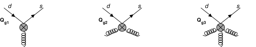
Here new operators have emerged

$$T = \left(L\otimes L+R\otimes R-\sigma_{\mu\nu}\otimes\sigma^{\mu\nu}\right)\frac{N-1}{2N}\leavevmode\hbox{\small 1\kern-3.8pt\normalsize 1}$$ (14a)

$$U = \frac{1}{2}\left(\gamma_{\mu}L\otimes\gamma^{\mu}R+\gamma_{\mu}R\otimes\gamma^{\mu}L\right)\left(\frac{N^{2}+N-1}{2N}\leavevmode\hbox{\small 1\kern-3.8pt\normalsize 1}-\frac{1}{2N}\widetilde{\leavevmode\hbox{\small 1\kern-3.8pt\normalsize 1}}\right)$$ (14b)

$$-\left(L\otimes R+R\otimes L\right)\left(\frac{N^{2}+N-1}{2N}\widetilde{\leavevmode\hbox{\small 1\kern-3.8pt\normalsize 1}}-\frac{1}{2N}\leavevmode\hbox{\small 1\kern-3.8pt\normalsize 1}\right),$$

which are written in a manifestly Fierz self-conjugate way. In the following we will discuss the coefficient functions $h$ in (13) in great detail, starting with those of the new operators:

$$h^{ct}_{T}\;=\;h_{T}\,S(x_{c},x_{t}); \qquad\qquad h^{j}_{T}\;=\;h_{T}\,S(x_{j}),\qquad j=c,t;$$ (15a)

$$h^{ct}_{U}\;=\;h_{U}\,S(x_{c},x_{t}); \qquad\qquad h^{j}_{U}\;=\;h_{U}\,S(x_{j}),\qquad j=c,t;$$ (15b)

$$h_{T}\;=\;-3-\xi; \qquad\qquad h_{U}\;=\;\frac{3+\xi}{2}\,\frac{m_{d}m_{s}}{m_{s}^{2}-m_{d}^{2}}\,\ln\frac{m_{s}^{2}}{m_{d}^{2}}.$$ (15c)

We first observe that (13) is obviously unphysical, because the functions in (15) are gauge dependent. This is an artifact of the use of small quark masses to regularize the infrared singularities while at the same time using on-shell quarks with zero four-momentum for the external states. For the same reason we encounter the new operators $T$ and $U$. Yet the one-loop matrix element of $\tilde{Q}_{S2}$ corresponding to the Feynman diagrams of Fig. 4

 

Figure 4: The classes of diagrams constituting the $O(\alpha_{s})$-contribution to the matrix element of $\tilde{Q}_{S2}$; the remaining diagrams are obtained by mirror reflections. The cross denotes the insertion of $\tilde{Q}_{S2}$, the curly lines gluons. A QCD counterterm has to be included.

 

involves the same operators (14) with the same coefficients [15, 16, 21]:

$$\langle\tilde{Q}_{S2}\left(\mu\right)\rangle\! = \!\langle\tilde{Q}_{S2}\left(\mu\right)\rangle^{(0)}+\frac{\alpha_{s}\left(\mu\right)}{4\pi}\left[a(\mu)\langle\tilde{Q}_{S2}\rangle^{(0)}+h_{T}\langle\hat{T}\rangle^{(0)}+h_{U}\langle\hat{U}\rangle^{(0)}\right].$$ (16)

We will discuss the third coefficient $a(\mu)$ in conjunction with $h^{j}$ in (13). Now (13) and (16) allow to express $i\widetilde{G}^{j}$ as

$$i\widetilde{G}^{j}(\mu) = \frac{\,G_{F}^{2}}{16\pi^{2}}M_{W}^{2}\left[S\left(x_{j}(\mu)\right)+\frac{\alpha_{s}(\mu)}{4\pi}k^{j}\left(x_{j}(\mu),\mu\right)\right]\langle\tilde{Q}_{S2}(\mu)\rangle$$ (17a)

$$+O(\alpha_{s}^{2}),\hskip 120.00018ptj=c,t,$$

$$i\widetilde{G}^{ct}(\mu) = \frac{\,G_{F}^{2}}{16\pi^{2}}M_{W}^{2}\left[S\left(x_{c}(\mu),x_{t}(\mu)\right)+\frac{\alpha_{s}(\mu)}{4\pi}k^{ct}\left(x_{c}(\mu),x_{t}(\mu),\mu\right)\right]\langle\tilde{Q}_{S2}(\mu)\rangle$$ (17b)

$$+O(\alpha_{s}^{2}),$$

where the new coefficient $k^{j}$ is related to $h^{j}$ in (13) and $a(\mu)$ in (16) via

$$h^{j} = k^{j}(x_{j},\mu)+a(\mu)S(x_{j}),\hskip 20.00003ptj=c,t,$$ (18a)

$$h^{ct} = k^{ct}(x_{c},x_{t},\mu)+a(\mu)S(x_{c},x_{t}).$$ (18b)

Now the unphysical terms $h_{T}$ and $h_{U}$ containing $\xi$ and the infrared regulators $m_{d}$ and $m_{s}$ have been absorbed into $\langle\tilde{Q}_{S2}\rangle^{(1)}$ in (17). Likewise these unphysical terms in $h^{j}$ have gone into $a(\mu)$ in (18), so that $k^{j}$ only depends on $x_{c}$, $x_{t}$ and $\mu$.

In the coefficient $a(\mu)$ in (16) we also split off the gauge and IR parts:

$$a(\mu) = c+\frac{N-1}{2N}6\ln\frac{m_{d}m_{s}}{\mu^{2}}$$

$$+2\xi\left[\left(C_{F}+\frac{N-1}{2N}\right)\left(1-\frac{m_{s}^{2}\ln\frac{m_{s}^{2}}{\mu^{2}}-m_{d}^{2}\ln\frac{m_{d}^{2}}{\mu^{2}}}{m_{s}^{2}-m_{d}^{2}}\right)+\frac{N-1}{2N}\ln\frac{m_{d}m_{s}}{\mu^{2}}\right],$$

$$c = -3\,C_{F}-5\,\frac{N-1}{2N}.$$ (19)

Next we write down the results for the $k^{j}$’s grouped according to powers of the large logarithm $\ln x_{c}$:

$$k^{ct}(x_{c},x_{t},\mu) = C_{F}\Biggl{[}-3x_{c}\ln^{2}x_{c}+x_{c}\ln x_{c}\left(-5-6\ln\frac{\mu^{2}}{m_{c}^{2}}+k^{ct}_{sing,a}\left(x_{t}\right)\right)$$ (20a)

$$\hskip 20.00003pt+x_{c}k^{ct}_{sing}\left(x_{t}\right)+x_{c}\ln\frac{\mu^{2}}{m_{c}^{2}}k^{ct}_{sing,a}\left(x_{t}\right)\Biggr{]}$$

$$+\frac{N-1}{2N}\Biggl{[}-9x_{c}\ln^{2}x_{c}+x_{c}\ln x_{c}\left(3+k^{ct}_{oct,a}\left(x_{t}\right)-6\ln\frac{\mu^{2}}{m_{c}^{2}}\right)$$

$$\hskip 40.00006pt+x_{c}k^{ct}_{oct}\left(x_{t}\right)+x_{c}\ln\frac{\mu^{2}}{m_{c}^{2}}k^{ct}_{oct,a}\left(x_{t}\right)\Biggr{]}$$

$$+c\,x_{c}\ln x_{c}-c\,x_{c}F(x_{t})+O\left(x_{c}^{2}\ln^{2}x_{c}\right),$$

$$k^{c}(x_{c},\mu) = C_{F}\left[-x_{c}+6x_{c}\ln\frac{\mu^{2}}{m_{c}^{2}}\right]$$ (20b)

$$+\frac{N-1}{2N}\Biggl{[}12x_{c}\ln x_{c}+6x_{c}\ln\frac{\mu^{2}}{m_{c}^{2}}-11x_{c}+\frac{4\pi^{2}}{3}x_{c}\Biggr{]}$$

$$-c\,x_{c}+O\left(x_{c}^{2}\right),$$

$$k^{t}(x_{t},\mu) = C_{F}\left[k^{t}_{sing}\left(x_{t}\right)+6\ln\frac{\mu^{2}}{M_{W}^{2}}k^{t}_{sing,a}\left(x_{t}\right)\right]$$ (20c)

$$+\frac{N-1}{2N}\Biggl{[}k^{t}_{oct}\left(x_{t}\right)+6\ln\frac{\mu^{2}}{M_{W}^{2}}S\left(x_{t}\right)\Biggr{]}-c\,S(x_{t}).$$

We have hidden a complicated $x_{t}$ dependence in the following functions:

$$k^{ct}_{sing}\left(x_{t}\right) = -3x_{t}\frac{7+7x_{t}+2x_{t}^{2}}{4\left(x_{t}-1\right)^{2}}+\pi^{2}\frac{-8+x_{t}^{2}}{4}$$ (21a)

$$+3x_{t}^{2}{\,\mathrm{Li}}_{2}\left(1-x_{t}\right)\frac{-2-2x_{t}+x_{t}^{2}}{2\left(1-x_{t}\right)^{2}}$$

$$+\ln x_{t}\frac{20-12x_{t}-51x_{t}^{2}-11x_{t}^{3}+6x_{t}^{4}}{4\left(1-x_{t}\right)^{3}}$$

$$+3\ln^{2}x_{t}\frac{4-12x_{t}-x_{t}^{2}-x_{t}^{3}-3x_{t}^{4}+x_{t}^{5}}{4\left(x_{t}-1\right)^{3}},$$

$$k^{ct}_{oct}\left(x_{t}\right) = \frac{-32+8x_{t}+3x_{t}^{2}}{4x_{t}\left(x_{t}-1\right)}+\pi^{2}\frac{-8-7x_{t}^{2}+x_{t}^{3}}{6x_{t}^{2}}$$ (21b)

$$+{\,\mathrm{Li}}_{2}\left(1-x_{t}\right)\frac{8-16x_{t}+23x_{t}^{2}-29x_{t}^{3}+4x_{t}^{4}+x_{t}^{5}}{x_{t}^{2}\left(x_{t}-1\right)^{2}}$$

$$+\ln x_{t}\frac{-32+36x_{t}-12x_{t}^{2}-7x_{t}^{3}}{4x_{t}\left(x_{t}-1\right)^{2}}$$

$$+\ln^{2}x_{t}\frac{12-16x_{t}+5x_{t}^{2}+2x_{t}^{3}}{4\left(x_{t}-1\right)^{2}},$$

$$k^{t}_{sing}\left(x_{t}\right) = x_{t}\frac{4-39x_{t}+168x_{t}^{2}+11x_{t}^{3}}{4\left(x_{t}-1\right)^{3}}+3x_{t}^{3}{\,\mathrm{Li}}_{2}\left(1-x_{t}\right)\frac{5+x_{t}}{\left(x_{t}-1\right)^{3}}$$ (21c)

$$+3x_{t}\ln x_{t}\frac{-4+24x_{t}-36x_{t}^{2}-7x_{t}^{3}-x_{t}^{4}}{2\left(x_{t}-1\right)^{4}}$$

$$+3x_{t}^{3}\ln^{2}x_{t}\frac{13+4x_{t}+x_{t}^{2}}{2\left(x_{t}-1\right)^{4}},$$

$$k^{t}_{oct}\left(x_{t}\right) = \frac{-64+68x_{t}+17x_{t}^{2}-11x_{t}^{3}}{4\left(1-x_{t}\right)^{2}}+\pi^{2}\frac{8}{3x_{t}}$$ (21d)

$$+2{\,\mathrm{Li}}_{2}\left(1-x_{t}\right)\frac{8-24x_{t}+20x_{t}^{2}-x_{t}^{3}+7x_{t}^{4}-x_{t}^{5}}{x_{t}\left(x_{t}-1\right)^{3}}$$

$$+\ln x_{t}\frac{-32+68x_{t}-32x_{t}^{2}+28x_{t}^{3}-3x_{t}^{4}}{2\left(x_{t}-1\right)^{3}}$$

$$+x_{t}^{2}\ln^{2}x_{t}\frac{4-7x_{t}+7x_{t}^{2}-2x_{t}^{3}}{2\left(x_{t}-1\right)^{4}},$$

$$k^{ct}_{sing,a}\left(x_{t}\right) = -9\frac{x_{t}}{\left(x_{t}-1\right)^{2}}+3\ln x_{t}\frac{-4+12x_{t}-3x_{t}^{2}+x_{t}^{3}}{2\left(x_{t}-1\right)^{3}},$$ (21e)

$$= 6\left(F(x_{t})-1+x_{t}\frac{d}{dx_{t}}F(x_{t})\right),$$

$$k^{ct}_{oct,a}\left(x_{t}\right) = \frac{9}{2}\frac{x_{t}}{x_{t}-1}+3\frac{4-8x_{t}+x_{t}^{2}}{2\left(1-x_{t}\right)^{2}}\ln x_{t}\;=\;6\,F(x_{t})$$ (21f)

$$k^{t}_{sing,a}\left(x_{t}\right) = x_{t}\frac{-4+18x_{t}+3x_{t}^{2}+x_{t}^{3}}{4\left(x_{t}-1\right)^{3}}-\frac{9x_{t}^{3}}{2\left(x_{t}-1\right)^{4}}\ln x_{t}$$ (21g)

$$= x_{t}\frac{d}{dx_{t}}S(x_{t}).$$

Here ${\,\mathrm{Li}}_{2}\left(x\right)$ denotes the dilogarithm function

$${\,\mathrm{Li}}_{2}\left(x\right) = -\int_{0}^{1}dt\frac{\ln\left(1-xt\right)}{t}$$ (22)

and $F(x_{t})$ has been defined in (10). Let us now look at the ingredients of (17) in more detail: (17) is an operator product expansion (OPE) of the Standard Model amplitude in terms of the local $\mathrm{|\Delta S|\!=\!2}$ operator $\tilde{Q}_{S2}$. The terms in brackets are the corresponding Wilson coefficients, yet in ordinary perturbation theory without any RG improvement. From (9) and (20) one verifies that they are gauge-independent and free of the infrared regulators $m_{s}$ and $m_{d}$. If we had used the dimensional method also to regularize the IR singularities, the operators $T$ and $U$ and the gauge dependence would be absent on both sides of (17), but the $k^{j}$’s would be unchanged. Further the Wilson coefficients do not depend on the choice of the external states used in the calculation of the matrix element. Now $k^{t}(x_{t},\mu)$ is simply the $O(\alpha_{s})$ part of the initial condition for the RG improved Wilson coefficient needed for the calculation of $\eta_{2}$. $k^{t}(x_{t},\mu)$ is called $D(x_{t})$ in [15]. The RG evolution from $\mu=M_{W}$ down to a low hadronic scale sums $\alpha_{s}\ln(\mu/M_{W})$ to all orders in perturbation theory. The situation would be the same with $k^{ct}$ and $k^{c}$ in a fictitious world in which the charm quark is so heavy that $\ln x_{c}$ is small. To describe the real nature, however, we must first sum $\alpha_{s}\ln x_{c}$ to all orders as well. Since this is the purpose of the subsequent sections, we discuss the powers of $\ln x_{c}$ term-by-term now. Therefore we have arranged (20) such that large logarithms can easily be distinguished from small terms.

$k^{ct}$:

In (20a) one immediately observes two terms $\propto\ln^{2}x_{c}$, which we have expected from the fact that $S(x_{c},x_{t})$ in (9c) already contains the logarithm $\ln x_{c}$. They all belong to the LO of RG improved perturbation theory, c.f. Table 1. Further $k^{ct}$ exhibits $\ln^{1}x_{c}$ terms. They are linked to the $\ln^{0}x_{c}$ term of $S(x_{c},x_{t})$ and constitute the first terms of the NLO expression. Note that the LO terms, the one $\propto\ln x_{c}$ in $S(x_{c},x_{t})$ and the $\ln^{2}x_{c}$ term of $k^{ct}$, are independent of $m_{t}$. Top dependence first enters through the NLO terms $\ln^{0}x_{c}$ in (9c) and the functions $k^{ct}_{sing,a}$ and $k^{ct}_{oct,a}$. Finally $k^{ct}$ contains a $\ln^{0}x_{c}$ piece, which already belongs to the next-to-next-to-leading order (NNLO). Therefore we will not need it in our analysis.

$k^{t}$:

(20c) contains the logarithm $\ln\mu^{2}/M_{W}^{2}$, which gets large when $\mu$ gets small. We expect the appearance of just this logarithm, because there are no other largely separated mass scales in $\widetilde{G}^{t}$. The whole $S(x_{t})$ in (9a) and the term $\propto\ln\mu^{2}/M_{W}^{2}$ in (20c) belong to the LO. The $\ln^{0}\mu^{2}/M_{W}^{2}$ part of (20c) is a NLO term.

$k^{c}$:

In (20b) we find the large logarithm $\ln x_{c}$, which together with $S(x_{c})$ belongs to the LO terms in $\widetilde{G}^{c}$. Note that the bracket proportional to $C_{F}$ does not contain such a logarithm, although the analogous term of $k^{t}$ contains one. This term is connected with the running of the corresponding quark mass. This mass is small in $\widetilde{G}^{c}$ but large in $\widetilde{G}^{t}$. The non-logarithmic part of (20b) again belongs to the NLO.

To gain an impression of the relevance of a calculation beyond the LO, we further look at the numerical sizes of the $S$- and $k$-functions. For typical values of the input parameters we obtain the numbers summarized in Table 2.

 

	$S^{j}$		$\displaystyle\frac{\alpha_{s}\left(m_{c}\right)}{4\pi}k^{j}$
$j$	$\ln^{1}$	$\ln^{0}$	$\ln^{2}$	$\ln^{1}$	$\ln^{0}$
$ct$	$0.002176$	$0.000311$	$-0.002766$	$0.000203$	$-0.000235$
$c$	$0$	$0.000264$	$0$	$-0.000192$	$0.000029$
$t$	$0$	$6.18$	$0$	$-9.21$	$-3.16$

Table 2: Numerical values of different contributions to the full SM amplitude. The listed values correspond to the case that $\alpha_{s}$ and $m_{t}$ are evolved down to $\mu=m_{c}$ without integrating out heavy degrees of freedom. We have split the $S$- and $k$-functions according to the power of $\ln x_{c}$ involved. We use $\alpha_{s}^{[f=6]}(m_{c})=0.277$ and $m_{t}^{[f=6]}(m_{c})=309\,\mathrm{GeV}$ corresponding to $f=6$ active flavours and typical values for $\alpha_{s}(M_{Z})$ and $m_{t}(m_{t})$. The $\alpha_{s}^{1}\ln^{n}x_{c}$-parts are of the same size as the $\alpha_{s}^{0}\ln^{n-1}x_{c}$-terms illustrating the need to sum $\alpha_{s}\ln x_{c}$ to all orders in perturbation theory as described in sect. 3.

 

Generally the $\alpha_{s}^{1}\ln^{n+1}$, $n=0,1$, terms are linked to the $\alpha_{s}^{0}\ln^{n}$ terms via the RG equation, cf. Table 1. In Table 2 one observes that the size of the $\alpha_{s}^{1}\ln^{n+1}$ contribution is about as large as the $\alpha_{s}^{0}\ln^{n}$ one. This emphasizes the need for the summation of large logarithms to all orders by means of an operator product expansion (OPE) and RG techniques. The thereby improved result will contain the coefficients of the logarithms listed in Table 2 evaluated for $\mu=\mu_{tW}=O(m_{t},M_{W})$. For example one finds for $\mu=m_{t}(m_{t})=167\,\mathrm{GeV}$:

$$\frac{1}{x_{c}}S(x_{c},x_{t}) = -\ln x_{c}+0.59$$ (23a)

$$\frac{1}{x_{c}}\frac{\alpha_{s}(\mu)}{4\pi}k^{ct}(x_{c},x_{t},\mu) = 0.026\ln^{2}x_{c}-0.22\ln x_{c}-0.27.$$ (23b)

The large magnitudes of the NLO coefficients 0.59 and $-0.22$ compared to the LO terms further emphasize the importance of the NLO calculation. Finally the constant term $-0.27$ enters the initial condition of the NNLO calculation. It amounts to 46% of the corresponding NLO term 0.59. The discussed initial condition, however, has a much smaller impact on the complete NLO result for $\eta_{3}$ than the operator mixing worked out in the following section.

3 Effective $\mathbf{\mathrm{|\Delta S|\!=\!2}}$ Transitions above the Charm Threshold

In this section we will sum the large logarithm $\ln x_{c}$ found in (9c) and (20) to all orders in perturbation theory. This is done in two steps: First one sets up an effective lagrangian $\mathcal{L}_{\mathrm{eff}}$ in which the W-boson and the top quark are removed as dynamic degrees of freedom. In $\mathcal{L}_{\mathrm{eff}}$ the $\mathrm{|\Delta S|\!=\!1}$ and $\mathrm{|\Delta S|\!=\!2}$ transitions are described by local four-quark operators, which are multiplied by Wilson coefficients. The logarithm $\ln x_{c}$ is thereby split as $\ln x_{c}=\ln(\mu^{2}/M_{W}^{2})+\ln(m_{c}^{2}/\mu^{2})$. Here the former term resides in the Wilson coefficients, which are functions of $m_{t}$, $M_{W}$ and $\mu$, and the latter is contained in the matrix elements of the four-quark operators depending only on $\mu$ and the light mass parameters. The second step is the application of the RG to the Wilson coefficients. For $\mu=\mu_{tW}=O(M_{W},m_{t})$ there is no large logarithm in the Wilson coefficients. The RG evolution from $\mu_{tW}$ down to $\mu_{c}=O(m_{c})$ sums $\ln(\mu_{c}^{2}/\mu_{tW}^{2})$ to all orders in perturbation theory. The RG improved coefficients finally multiply matrix elements which do not contain large logarithms, because $\ln(m_{c}^{2}/\mu_{c}^{2})$ is small.

When passing with $\mu$ below $\mu_{c}$ we must also integrate out the c-quark field. This will be described in sect. 4.

3.1 General Structure of the Effective Lagrangian

After integrating out the top quark and the W-boson we are left with an effective five-flavour theory described by a lagrangian of the generic form

$$\mathcal{L}_{\mathrm{eff}}^{\mathrm{|\Delta S|\!=\!2}} = -\frac{\,G_{F}}{\sqrt{2}}V_{\mathrm{CKM}}\sum_{k}C_{k}Q_{k}-\frac{\,G_{F}^{2}}{2}V_{\mathrm{CKM}}\sum_{l}\widetilde{C}_{l}\widetilde{Q}_{l}.$$ (24)

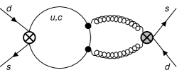
Here the $V_{\mathrm{CKM}}$ denotes products of CKM elements. The $Q_{k}$, $\widetilde{Q}_{l}$ represent local $\mathrm{|\Delta S|\!=\!1}$ and $\mathrm{|\Delta S|\!=\!2}$ operators and the $C_{k}$, $\widetilde{C}_{l}$ are the corresponding Wilson coefficient functions with Fermi’s constant factored out. The $\mathrm{|\Delta S|\!=\!1}$ operators $Q_{k}$ are necessary for the proper treatment of $\mathrm{|\Delta S|\!=\!2}$ transitions, because they contribute to the transition amplitude through Green’s functions with two operator insertions. An example is shown in Fig. 5, which is simply obtained from Fig. 2 by shrinking the W-boson lines to a point.

 

Figure 5: Diagram $\mathsf{D_{0}}$ in the effective five- and four-quark theory. The crosses denote insertions of local $\mathrm{|\Delta S|\!=\!1}$ current-current operators.

 

The $\mathrm{|\Delta S|\!=\!2}$ operators $\widetilde{Q}_{k}$ (see e.g. Fig. 2) can likewise be obtained by shrinking the whole box function with internal top quarks in Fig. 2 to a point. Yet the $\widetilde{Q}_{k}$’s are also needed for the light quark contributions. Diagrams of the type in Fig. 5 are in general divergent and require counterterms (omitted in (24)) proportional to $\mathrm{|\Delta S|\!=\!2}$ operators. In general both $\mathrm{|\Delta S|\!=\!1}$ and $\mathrm{|\Delta S|\!=\!2}$ operators in (24) contribute to $\mathrm{|\Delta S|\!=\!2}$ transitions. Yet there may be special cases in which either the former or the latter are absent. As we will see later, all three possibilities are realized in $\eta_{1}$, $\eta_{2}$ and $\eta_{3}$.

In the following sections the detailed structure of ${\mathcal{L}_{\mathrm{eff}}^{\mathrm{|\Delta S|\!=\!2}}}$ will be worked out. This requires the following steps:

1. Find the minimal operator basis to be used in (24) sufficient to describe the physics of the $\mathrm{|\Delta S|\!=\!2}$ transition. Here one must first find a set of operators closing under renormalization. Subsequently one can eliminate a set of unphysical operators.

2. Match the full SM Green’s function $\widetilde{G}$ of (4), (5), (7) and (17) to the one obtained in the effective theory and thereby determine the Wilson coefficient functions $C_{k}$ and $\widetilde{C}_{l}$ at the initial scale $\mu=\mu_{tW}=O(M_{W},m_{t})$.

3. Next prepare for the RG evolution of the Wilson coefficients from $\mu=\mu_{tW}$ down to the final scale $\mu=\mu_{c}=O(m_{c})$. For this one must derive the general RG equation for Green’s functions with double insertions (see Fig. 5) and its solution. The RG equation involves an anomalous dimension tensor in addition to the familiar anomalous dimension matrices.

4. Determine the anomalous dimension tensor in the NLO for the operator basis at hand. This requires the calculation of two-loop diagrams.

Finally we discuss the size of the remaining non-summed logarithm $\ln m_{t}/M_{W}$. We do not sum this logarithm because we simultaneously integrate out the top quark and the W-boson.

3.2 The Operator Basis

At first we restrict the set of operators in (24) to the lowest contributing dimension, which means dimension six for the $Q_{k}$’s. As for the $\widetilde{Q}_{l}$’s, we must distinguish whether they correspond to the SM graphs with internal top quarks or whether they enter ${\mathcal{L}_{\mathrm{eff}}^{\mathrm{|\Delta S|\!=\!2}}}$ as counterterms in the light quark sector. In the former case there is only one physical $\mathrm{|\Delta S|\!=\!2}$ operator $\tilde{Q}_{S2}$, introduced in (2), with a dimension-two Wilson coefficient $\widetilde{C}_{S2}^{(t)}$ containing all information on $m_{t}$ and $M_{W}$ [15]. The latter operators have the same dimension as the diagrams they renormalize, which is eight as can be easily seen from Fig. 5. Higher dimension operators correspond to terms suppressed by powers of $m^{2}_{\mathrm{light}}/m^{2}_{\mathrm{heavy}}$, which we already neglected in the SM amplitude, see (9) and (20).

We will now establish the $\mathrm{|\Delta S|\!=\!1}$ part of the operator basis, i.e. the $Q_{k}$’s in (24). Consider first the SM $\mathrm{|\Delta S|\!=\!1}$ transition of Fig. 7 with only light quarks $k,l=u,c$ on the external legs. Contracting the W-boson propagator to a point yields the diagram of Fig. 7, in which the cross denotes the insertion of the $\mathrm{|\Delta S|\!=\!1}$ current-current operator

$$Q_{2}^{kl} = \left(\bar{s}\gamma_{\mu}Lk\right)\cdot\left(\bar{l}\gamma^{\mu}Ld\right)\cdot\leavevmode\hbox{\small 1\kern-3.8pt\normalsize 1},$$ (25)

which we have already met in Fig. 5.

 

Figure 6: A $\mathrm{|\Delta S|\!=\!1}$ transition in the standard model.

Figure 7: The matrix element of a $\mathrm{|\Delta S|\!=\!1}$ current-current operator $Q_{1,2}^{kl}$ displayed as the cross.

 

It is well-known that QCD corrections to $Q_{2}^{kl}$ induce counterterms proportional to other operators, so that $Q_{2}^{kl}$ mixes with them under renormalization.

In the case of $k\neq l$ the mixing is particularly simple, $Q_{2}^{kl}$ only mixes with

$$Q_{1}^{kl} = \left(\bar{s}\gamma_{\mu}Lk\right)\cdot\left(\bar{l}\gamma^{\mu}Ld\right)\cdot\widetilde{\leavevmode\hbox{\small 1\kern-3.8pt\normalsize 1}}.$$ (26)

The one-loop mixing proceeds through the diagrams of Fig. 8.

 

Figure 8: The classes of diagrams yielding the matrix element of the $\mathrm{|\Delta S|\!=\!1}$ current-current operators $Q_{1,2}^{kl}$ as well as the mixing of the current-current operators among themselves to order $\alpha_{s}$.

 

Hence the corresponding part of $\mathcal{L}_{\mathrm{eff}}^{\mathrm{|\Delta S|\!=\!2}}$ reads

$$-\frac{\,G_{F}}{\sqrt{2}}\sum_{i,j=1}^{2}\sum_{k,l=u,c}V_{ks}^{\ast}V_{ld}C_{i}Z^{-1}_{ij}Q_{j}^{kl,\,\mathrm{bare}}.$$ (27)

Here and in the following the superscript “bare” denotes unrenormalized operators, while renormalized ones do not carry an additional superscript. The 2$\times$2 renormalization matrix $Z^{-1}_{ij}$ is diagonal in the basis

$$Q_{\pm}^{kl} = \frac{1}{2}\left(Q_{2}^{kl}\pm Q_{1}^{kl}\right),$$ (28)

provided one preserves Fierz symmetry in the renormalization process [21, 33].

For $k=l$ additional operators enter the scene, the so-called $\mathrm{|\Delta S|\!=\!1}$ penguin operators, which appear in different species. In [24, 25] the NLO mixing of $Q_{1,2}$ with quark-foot penguin operators $Q_{3}$ to $Q_{6}$ displayed in Fig. 10 has been worked out. They read

$$Q_{3} = \left(\overline{s}\gamma_{\mu}Ld\right)\cdot\sum_{q=d,u,s,\ldots}\left(\overline{q}\gamma^{\mu}Lq\right)\cdot\leavevmode\hbox{\small 1\kern-3.8pt\normalsize 1}$$

$$Q_{4} = \left(\overline{s}\gamma_{\mu}Ld\right)\cdot\sum_{q=d,u,s,\ldots}\left(\overline{q}\gamma^{\mu}Lq\right)\cdot\widetilde{\leavevmode\hbox{\small 1\kern-3.8pt\normalsize 1}}$$

$$Q_{5} = \left(\overline{s}\gamma_{\mu}Ld\right)\cdot\sum_{q=d,u,s,\ldots}\left(\overline{q}\gamma^{\mu}Rq\right)\cdot\leavevmode\hbox{\small 1\kern-3.8pt\normalsize 1}$$

$$Q_{6} = \left(\overline{s}\gamma_{\mu}Ld\right)\cdot\sum_{q=d,u,s,\ldots}\left(\overline{q}\gamma^{\mu}Rq\right)\cdot\widetilde{\leavevmode\hbox{\small 1\kern-3.8pt\normalsize 1}}$$ (29)

and enter (24) with $V_{\mathrm{CKM}}=-\lambda_{t}$. The summation runs over all active flavours, at present $q=d,u,s,c$ and $b$.

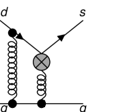
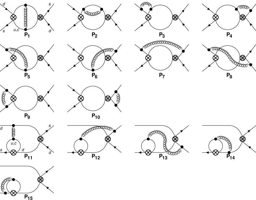
Yet we may doubt, whether $Q_{1}-Q_{6}$ are sufficient to describe the $\mathrm{|\Delta S|\!=\!1}$ substructure in $\mathrm{|\Delta S|\!=\!2}$ transition. Indeed, $Q_{1}-Q_{6}$ mix via the diagrams of Fig. 11 into operators containing only two quark lines such as the gluon-foot penguin operators $Q_{g1}$, $Q_{g2}$ and $Q_{g3}$ depicted in Fig. 12. Likewise loop diagrams with $Q_{g1}-Q_{g3}$ require counterterms proportional to $Q_{3}-Q_{6}$ (see Fig. 10) and similarly to a ghost-foot penguin operator

$$Q_{\mathrm{FP}} = \overline{s}\gamma_{\mu}LT^{a}d\cdot\left(\partial^{\mu}\overline{\eta}^{b}\right)\eta^{c}f^{abc}.$$ (30)

Here $\eta_{c}$ denotes a Faddeev-Popov ghost field. We can easily construct a $\mathrm{|\Delta S|\!=\!2}$ diagram with one of these operators and $Q_{2}$, see e.g. Fig. 13.

 

Figure 9: The four-quark penguin operators $Q_{3,\ldots,6}$

Figure 10: Diagrams for the mixing of $Q_{g1}$ denoted by the shaded cross into four-quark penguin operators.

 

 

Figure 11: The mixing of a $\mathrm{|\Delta S|\!=\!1}$ current-current operator, denoted by the cross, into gluon-penguin operators. Diagrams with the gluon lines permuted compared to $\mathsf{G_{2}}$ and $\mathsf{G_{3}}$ must be included, too.

 

 

Figure 12: The $\mathrm{|\Delta S|\!=\!1}$ gluon-foot penguin operators

 

 

Figure 13: $\mathrm{|\Delta S|\!=\!2}$ diagram with one insertion of $Q_{1,2}$, denoted by the light cross, and $Q_{g2}$, denoted by the shaded cross, which could contribute to $\eta_{3}$.

 

Fortunately these extra operators $Q_{g1}-Q_{g3}$, $Q_{\mathrm{FP}}$ combine to unphysical operators, which can be dropped from the renormalized effective lagrangian [26, 27, 28, 29, 30]. Hence the $\mathrm{|\Delta S|\!=\!1}$ operators in (24) can be restricted to $Q_{1}^{kl},\ldots,Q_{6}$ and the $\mathrm{|\Delta S|\!=\!1}$ part of $\mathcal{L}_{\mathrm{eff}}^{\mathrm{|\Delta S|\!=\!2}}$ reads

$${\mathcal{L}}^{\mathrm{|\Delta S|=1}} = -\frac{\,G_{F}}{\sqrt{2}}\left[\sum_{i=1}^{2}\sum_{k,l=u,c}V_{ks}^{\ast}V_{ld}C_{i}Q_{i}^{kl}-\lambda_{t}\sum_{j=3}^{6}C_{j}Q_{j}\right].$$ (31)

We will illustrate the irrelevance of $Q_{g1}-Q_{g3},Q_{\mathrm{FP}}$ in the following section. This, however, first requires the determination of the local $\mathrm{|\Delta S|\!=\!2}$ operators $\widetilde{Q}_{l}$ in (24).

Consider first the simplest case, which is realized in $\widetilde{G}^{t}$: the SM result for $\widetilde{G}^{t}$ is proportional to the square of a heavy mass $m_{t}$, $M_{W}$ times a function of their ratios (see (7b), (13) with $j=t$). A diagram in the effective five-flavour theory containing two insertions of $\mathrm{|\Delta S|\!=\!1}$ operators can only produce a result involving light mass parameters, which we already neglected in (7b), (13). Therefore the diagrams with double insertions do not contribute in this case and we are left with a $\mathrm{|\Delta S|\!=\!2}$ contribution to $\mathcal{L}_{\mathrm{eff}}^{\mathrm{|\Delta S|\!=\!2}}$ of the form

$$-\frac{G_{F}^{2}}{2}\lambda_{t}^{2}\widetilde{C}_{S2}^{(t)}\tilde{Q}_{S2}.$$ (32)

$\widetilde{C}_{S2}^{(t)}$ has been obtained in the NLO in [15].

In the light quark sector the situation is a bit more involved: Consider first the diagram of Fig. 5 with two internal charm quarks and zero external momenta. The only physical dimension-eight $\mathrm{|\Delta S|\!=\!2}$ operators required to absorb its divergence reads

$$\widetilde{Q}_{7} = \frac{m_{c}^{2}}{g^{2}\mu^{2\varepsilon}}\tilde{Q}_{S2}=\frac{m_{c}^{2}}{g^{2}\mu^{2\varepsilon}}\cdot\overline{s}\gamma_{\mu}Ld\cdot\overline{s}\gamma^{\mu}Ld,$$ (33)

which follows from power counting and the absence of any non-zero mass parameter apart from $m_{c}$. The inverse powers of $g$ are introduced for later convenience as in [10]. One may arbitrarily shift such factors from the Wilson coefficient into the definition of the operator. The factor $\mu^{-2\varepsilon}$ stems from $g_{\mathrm{bare}}=Z_{g}g\mu^{\varepsilon}$ and the fact that

$$\widetilde{Q}_{7}^{\mathrm{bare}} = \frac{m_{c,\,\mathrm{bare}}^{2}}{g_{\mathrm{bare}}^{2}}\left[\overline{s}\gamma_{\mu}Ld\cdot\overline{s}\gamma^{\mu}Ld\right]^{\mathrm{bare}}.$$ (34)

must be independent of $\mu$. Any other dimension-eight $\mathrm{|\Delta S|\!=\!2}$ operator contains one or two powers of $m_{c}$ less than $\widetilde{Q}_{7}$ and derivatives and/or gluon fields instead. Their on-shell matrix elements are suppressed by powers of $m_{s}/m_{c}$ with respect to those of $\widetilde{Q}_{7}$, so that they do not contribute to the coefficient of the leading dimension-six operator below the charm threshold (cf. (1)). Likewise they cannot mix with $\widetilde{Q}_{7}$ under renormalization.

Next we determine the CKM factor multiplying $\widetilde{C}_{7}\widetilde{Q}_{7}$: Generally we could expect a term proportional to $\lambda_{c}^{2}$ and one proportional to $\lambda_{c}\lambda_{t}$ corresponding to $\widetilde{G}^{c}$ and $\widetilde{G}^{ct}$ respectively. Due to the special structure of $\widetilde{G}^{c}$, which does not contain a large logarithm to order $\alpha_{s}^{0}$ in the SM amplitude (9b), no term proportional to $\lambda_{c}^{2}\widetilde{Q}_{7}$ occurs.

Hence $\mathcal{L}_{\mathrm{eff}}^{\mathrm{|\Delta S|\!=\!2}}$ is found as

$${\mathcal{L}}_{\mathrm{eff}}^{\mathrm{|\Delta S|=2}} = -\frac{\,G_{F}}{\sqrt{2}}\sum_{i=1}^{6}C_{i}\left[\sum_{j=1}^{2}Z^{-1}_{ij}\sum_{k,l=u,c}V_{ks}^{\ast}V_{ld}Q_{j}^{kl,\,\mathrm{bare}}-\lambda_{t}\sum_{j=3}^{6}Z^{-1}_{ij}Q_{j}^{\mathrm{bare}}\right]$$ (35)

$$-\frac{\,G_{F}^{2}}{16\pi^{2}}\lambda_{t}^{2}\widetilde{C}_{S2}^{(t)}\widetilde{Z}_{S2}^{-1}\tilde{Q}_{S2}^{\mathrm{bare}}$$

$$-\frac{\,G_{F}^{2}}{2}\lambda_{c}\lambda_{t}\left[\sum_{k=1}^{2}\sum_{l=1}^{6}C_{k}C_{l}\widetilde{Z}_{kl,7}^{-1}+\widetilde{C}_{7}\widetilde{Z}_{77}^{-1}\right]\widetilde{Q}_{7}^{\mathrm{bare}}$$

$$+\textrm{counterterms proportional to unphysical operators}.$$

Here the first line is the pure $\mathrm{|\Delta S|\!=\!1}$ part (31) written in terms of bare operators and the corresponding renormalization factors. The second line contains everything related to a single insertion of the local $\mathrm{|\Delta S|\!=\!2}$ operator $\tilde{Q}_{S2}$. The third line consists of two parts: the counterterm involving $\widetilde{Z}^{-1}_{kl,7}$ renormalizes the matrix elements of the type in Fig. 5 or Fig. 14 with one insertion of $Q_{l}$ and one of $Q_{k}$. The part of (35) involving $\widetilde{Z}_{77}^{-1}$ expresses the renormalization of the local $\mathrm{|\Delta S|\!=\!2}$ operator $\widetilde{Q}_{7}$ in single insertions to cancel the divergences of the diagrams depicted in Fig. 4. The absence of a local $\mathrm{|\Delta S|\!=\!2}$ operator proportional to $\lambda_{c}^{2}$ in (35) is due to the GIM mechanism (see [10, 16]). The structure of (35) becomes much more transparent, if one regards the Z-factors as renormalization factors of the effective couplings $C_{l}$, $\widetilde{C}_{7}$ rather than of the operators. The bracket in the third line of (35) may then simply be interpreted as the “bare” Wilson coefficient of $\widetilde{Q}_{7}$ in analogy to the bare coupling in QCD. It is renormalized both by QCD and by effective $\mathrm{|\Delta S|\!=\!1}$ interactions. The last line of (35) contains counterterms proportional to unphysical operators, which are described in the next section. One automatically includes them in the calculation, if one simply subtracts the subdivergences diagram-by-diagram in the effective theory.

3.2.1 Unphysical Operators

We will discuss three types of unphysical operators: BRS-exact operators, those which vanish by a field equation of motion (EOM) and evanescent operators. Therefore let class $\mathcal{B}$ contain all BRS-exact operators, class $\mathcal{E}$ the operators vanishing by a field equation of motion and class $\mathcal{P}$ the physical and evanescent operators.

Let us first reduce the operator basis with respect to classes $\mathcal{B}$ and $\mathcal{E}$. The techniques to do this have been worked out in [26, 27, 28, 29, 30, 31]. They are widely used for the treatment of Green’s functions with single operator insertions. Here the new issue is the application of the theorems concerning double insertions [28, 30] in a concrete calculation.

The mixing of the classes introduced above follows the general pattern

$$Z^{-1}=\left(\begin{array}[]{ccc}*&*&*\\ 0&*&*\\ 0&0&*\end{array}\right)\hskip 30.00005pt\mbox{corresponding to class}\hskip 30.00005pt\left(\begin{array}[]{c}\mathcal{P}\\ \mathcal{B}\\ \mathcal{E}\end{array}\right).$$ (42)

The block-triangular form of (42) ensures that the Wilson coefficients of the operators from classes $\mathcal{B}$ and $\mathcal{E}$ do not mix into the ones of physical and evanescent operators in $\mathcal{P}$.

Further we know that the on-shell matrix elements of operators in class $\mathcal{B}$ or $\mathcal{E}$ vanish. This is important for the matching of transition amplitudes in different theories, e.g. of the full SM and of an effective five-flavour theory. The vanishing of the on-shell matrix elements of operators in $\mathcal{B}$ and $\mathcal{E}$ ensures that they do not contribute to physical Wilson coefficients at the matching scale.

Since operators from $\mathcal{B}$ and $\mathcal{E}$ contribute neither to the matching nor to the mixing of class $\mathcal{P}$, we may neglect them in the discussion of the RG equation and evolution.

Let us now organize the penguin zoo according to the classes $\mathcal{P}$, $\mathcal{B}$ and $\mathcal{E}$. Due to the theorems of [26, 27, 28, 29, 30, 31] the operators $Q_{g1}-Q_{g3},Q_{\mathrm{FP}}$ can be arranged to appear in the combinations

$$Q_{\mathrm{BRS}}=Q_{\mathrm{FP}}+Q_{\mathrm{gf}}\quad\in{\cal B}$$ (43)

and

$$Q_{\mathrm{g}{\mathrm{EOM}}} = Q_{\mathrm{g}}-\frac{1}{4}\left(Q_{4}+Q_{6}\right)+\frac{1}{4N}\left(Q_{3}+Q_{5}\right)-Q_{\mathrm{BRS}}\quad\in{\cal E}$$ (44)

with

$$Q_{\mathrm{g}}=\frac{1}{g}\bar{s}\gamma_{\mu}LT^{a}d\cdot D_{\nu}^{a}F^{\mu\nu},\qquad Q_{\mathrm{gf}}\;=\;\frac{1}{g}\frac{1}{\xi}\bar{s}\gamma_{\mu}LT^{a}d\cdot\partial^{\mu}\partial^{\nu}A^{a}_{\nu}.$$ (45)

The latter is stemming from the gauge fixing part of the QCD Lagrangian. $Q_{\mathrm{g}{\mathrm{EOM}}}$ vanishes by the equation of motion of the gluon field. $Q_{\mathrm{BRS}}$ and $Q_{\mathrm{g}{\mathrm{EOM}}}$ are discussed in detail in [30].

Since now $Q_{g1}-Q_{g3},Q_{\mathrm{FP}}$ have been traded for linear combination belonging to classes ${\cal E}$ and ${\cal B}$, one may drop them from the renormalized operator basis when calculating $\mathrm{|\Delta S|\!=\!1}$ transitions.

In the case of double insertions the situation is more complex, because now the operators of class $\mathcal{E}$ may give a nonzero contribution in on-shell matrix elements and therefore their presence cannot be ignored for the matching. Yet it is possible to absorb the effects of these operators into the coefficient of a $\mathrm{|\Delta S|\!=\!2}$ operator [31, 30]. Such non-vanishing matrix elements with two insertions of $Q_{\mathrm{g}{\mathrm{EOM}}}$ appear in $\widetilde{G}^{t}$ of (4). Since the effective five- or four-flavour theory does not contain $m_{t}$ and $M_{W}$ anymore, this contribution is suppressed by a factor of $m^{2}_{\mathrm{light}}/m^{2}_{\mathrm{heavy}}$ compared to the term in the second line of (35) and can therefore be neglected. Yet in the calculation of $\widetilde{G}^{ct}$ we will face the operator

$$Q_{\mathrm{q}{\mathrm{EOM}}} = m_{c}^{2}\,\overline{s}RD\hskip-8.55695pt\lower-0.91666pt\hbox to8.55695pt{\hss\sl/\/\hss}d,$$ (46)

which vanishes by the quark equation of motion. Its effect on $\mathrm{|\Delta S|\!=\!2}$ amplitudes can likewise be absorbed into $\widetilde{C}_{7}$.

On-shell matrix elements involving one or two operators from class $\mathcal{B}$ still vanish, we can therefore drop them in the case of double insertions, too.

Another important class of unphysical operators are the evanescent operators also contained in $\mathcal{P}$, which generally appear in theories with four-fermion interactions, if one uses dimensional regularization. As an example one may look at the $O(\alpha_{s})$ corrections to the matrix element of $Q_{1,2}$, displayed in Fig. 8. When calculating diagram $\mathsf{C_{2}}$, $\mathsf{C_{3}}$ one faces the structure

$$Q^{\prime} \!=\! \gamma_{\rho}\gamma_{\sigma}\gamma_{\mu}\left(1-\gamma_{5}\right)\otimes\gamma^{\mu}\gamma^{\sigma}\gamma^{\rho}\left(1-\gamma_{5}\right)=(4-a\varepsilon)Q+E_{1}[Q]+O(\varepsilon^{2}),$$ (47)

where $Q=\gamma_{\mu}L\otimes\gamma^{\mu}L$. $E_{1}[Q]$ is evanescent, i.e. it vanishes for $D=4$. $a$ is an arbitrary real parameter, its choice belongs to the definition (47) of $E_{1}[Q]$.

When perturbative results are improved by means of the OPE and RG techniques, subtleties arise: Evanescent operators can affect the matching procedure [21] and the operator mixing [31, 32]. In [31, 21] a finite renormalization of the evanescent operators has been proposed to render their matrix elements zero. Doing so the Wilson coefficients of the evanescent operators become irrelevant at the matching scale. If this should hold at any other scale, one has to ensure that the Wilson coefficients of the evanescent operators do not mix into the ones of the physical operators. This has been proven in [32] for a very special and calculationally inconvenient definition of the evanescent operators. In [33] we achieved the following improvements:

1. We have generalized the proof of [32] to an arbitrary definition of the evanescent operators, which includes the one chosen in [21].

2. We have shown that the arbitrariness in the definition of the evanescent operators displayed in (47) introduces a scheme dependence into the physical Wilson coefficients at the matching scale as well as into the physical anomalous dimension matrix starting in the NLO. This distinguishes the evanescent operators from the operators in classes ${\cal E}$ and ${\cal B}$. Of course this scheme dependence cancels in the product of Wilson coefficients and matrix elements at any scale. We give explicit formulae to transform Wilson coefficients or anomalous dimension matrices from one scheme to another. These formulae are particularly necessary if one wants to combine Wilson coefficients and anomalous dimension matrices calculated with different definitions of the evanescent operators.

3. We have extended the findings from the case of single insertions to double insertions, which is needed for this work.

It is important to note that the first and third point above enables us to use the results of [21, 24, 25] for the $\mathrm{|\Delta S|\!=\!1}$ hamiltonian in (31).

The physical operators in $\mathcal{P}$ needed in our calculation are

$$Q_{i}^{kl},\quad i=1,2,\quad k,l=u,c;\qquad\qquad Q_{j},\quad j=3,\ldots 6;\qquad\qquad\widetilde{Q}_{7}.$$ (48)

For the evanescent operators appearing in the calculation we use the definition:

$$E_{1}[Q_{j}] \!=\! \left[\gamma_{\mu}\gamma_{\nu}\gamma_{\eta}L\otimes\gamma^{\eta}\gamma^{\nu}\gamma^{\mu}L-\left(4+a_{1}\varepsilon\right)\gamma_{\mu}L\otimes\gamma^{\mu}L\right]K_{1j},\hskip 10.00002ptj=1,\ldots 4,$$ (49a)

$$E_{1}[Q_{j}] \!=\! \left[\gamma_{\mu}\gamma_{\nu}\gamma_{\eta}R\otimes\gamma^{\eta}\gamma^{\nu}\gamma^{\mu}L-\left(16+a_{2}\varepsilon\right)\gamma_{\mu}R\otimes\gamma^{\mu}L\right]K_{1j},\quad j=5,6,$$ (49b)

$$E_{1}[\widetilde{Q}_{7}] \!=\! \frac{m_{c}^{2}}{g^{2}}\left[\gamma_{\mu}\gamma_{\nu}\gamma_{\eta}L\otimes\gamma^{\eta}\gamma^{\nu}\gamma^{\mu}L-\left(4+\tilde{a}_{1}\varepsilon\right)\gamma_{\mu}L\otimes\gamma^{\mu}L\right]K_{12},$$ (49c)

$$E_{2}[\widetilde{Q}_{7}] \!=\! \frac{m_{c}^{2}}{g^{2}}\left[\gamma_{\mu}\gamma_{\nu}\gamma_{\eta}\gamma_{\sigma}\gamma_{\tau}L\otimes\gamma^{\tau}\gamma^{\sigma}\gamma^{\eta}\gamma^{\nu}\gamma^{\mu}L\right.$$ (49d)

$$\hskip 20.00003pt\left.-\left[\left(4+\tilde{a}_{1}\varepsilon\right)^{2}+\tilde{b}_{1}\varepsilon\right]\gamma_{\mu}L\otimes\gamma^{\mu}L\right]K_{22}.$$

Here $E_{1}[Q_{j}]$ is the evanescent operator needed as a counterterm to render the diagrams $\mathsf{C_{2}}$ and $\mathsf{C_{3}}$ in Fig. 8 with $Q_{j}$ inserted finite. The colour factors $K_{1j}$ are

$$K_{12}=K_{13}=K_{15} = \frac{1}{2}\widetilde{\leavevmode\hbox{\small 1\kern-3.8pt\normalsize 1}}-\frac{1}{2N}\leavevmode\hbox{\small 1\kern-3.8pt\normalsize 1},$$

$$K_{11}=K_{14}=K_{16} = \frac{1}{4}\leavevmode\hbox{\small 1\kern-3.8pt\normalsize 1}+\frac{N^{2}-2}{4N}\widetilde{\leavevmode\hbox{\small 1\kern-3.8pt\normalsize 1}}.$$ (50)

Likewise $E_{2}[\widetilde{Q}_{7}]$ appears in two-loop diagrams involving physical operators or in one-loop matrix elements of $E_{1}[\widetilde{Q}_{7}]$.

In our NLO calculation we have kept $a_{1}$, $a_{2}$, $\tilde{a}_{1}$ and $\tilde{b}_{1}$ arbitrary for two reasons: First we want to illustrate our findings of [33] in sect. 3.5.1. Second the vanishing of these quantities from physical results provides a non-trivial check of our calculation.

Apart from sect. 3.5.1 we will always state the results corresponding to

$$a_{1}=-8,\hskip 30.00005pta_{2}=-16,\hskip 30.00005pt\tilde{a}_{1}=-8,$$ (51)

in order to comply with the standard choice used in [21, 16, 15, 24, 25]. Since NLO anomalous dimensions and matching corrections of physical operators do not depend on $\tilde{b}_{1}$, we do not give a numerical value. Likewise we do not need the value of the colour factor $K_{22}$.

Let us finally look at the operator $\widetilde{Q}_{7}$ or equivalently at $\tilde{Q}_{S2}$ appearing in (35) and (1) to introduce a different type of evanescent operator: The Dirac and flavour structure of $\tilde{Q}_{S2}=(\overline{s}d)_{V-A}(\overline{s}d)_{V-A}\leavevmode\hbox{\small 1\kern-3.8pt\normalsize 1}$ is Fierz self-conjugate in four dimensions. Hence $\tilde{Q}_{S2}$ differs from its Fierz transform $(\overline{s}d)_{V-A}(\overline{s}d)_{V-A}\widetilde{\leavevmode\hbox{\small 1\kern-3.8pt\normalsize 1}}$ by an evanescent operator. In general we must therefore expect the NLO anomalous dimension to be different for $\tilde{Q}_{S2}$ and its Fierz transform. Yet the standard definition of $E_{1}[\tilde{Q}_{S2}]$ with $\widetilde{a}_{1}=-8$ ensures Fierz symmetry to hold at the loop level as well (see [21, 33]). Hence with the choice $\widetilde{a}_{1}=-8$ it does not matter whether one uses $\tilde{Q}_{S2}$ or its Fierz transform or any linear combination of them in the calculation. This is especially gratifying for the hamiltonian (1) below the charm threshold, if the non-perturbative methods used to obtain the matrix element of $\tilde{Q}_{S2}$ do not distinguish between $\tilde{Q}_{S2}$ and its Fierz transform.

3.2.2 Green’s Functions from $\mathbf{{\mathcal{L}}_{{\mathrm{eff}}}^{\mathrm{|\Delta S|\!=\!2}}}$

The following sections will deal with the determination of the Wilson coefficients and renormalization $Z$-factors present in (35). To do so we need to know the Green’s function obtained from ${\mathcal{L}}_{{\mathrm{eff}}}^{\mathrm{|\Delta S|\!=\!2}}$ to order $\,G_{F}^{2}$. It reads:

$$\!\!\left\langle\,\mathrm{\mathbf{T\,}}\exp\left[i\int d^{D}x{\mathcal{L}}^{\mathrm{|\Delta S|\!=\!2}}_{{\mathrm{eff}}}\left(x\right)\right]\right\rangle_{\mathrm{|\Delta S|\!=\!2}} = -i\left\langle H^{c}+H^{t}+H^{ct}\right\rangle+O\left(G_{F}^{3}\right),$$ (52)

where

$$H^{c}\left(x\right) = \lambda_{c}^{2}\frac{\,G_{F}^{2}}{2}\sum_{i,i^{\prime},j,j^{\prime}=+,-}C_{i}C_{j}\underbrace{Z^{-1}_{ii^{\prime}}Z^{-1}_{jj^{\prime}}\mathcal{O}^{\mathrm{bare}}_{i^{\prime}j^{\prime}}\left(x\right)}_{\displaystyle\equiv\mathcal{O}_{ij}\left(x\right)},$$ (53a)

$$H^{t}\left(x\right) = \lambda_{t}^{2}\frac{\,G_{F}^{2}}{16\pi^{2}}\widetilde{C}_{S2}^{(t)}\widetilde{Z}_{S2}^{-1}\tilde{Q}_{S2}^{\mathrm{bare}}\left(x\right),$$ (53b)

$$H^{ct}\left(x\right) = \lambda_{c}\lambda_{t}\!\Biggl{[}\frac{\,G_{F}^{2}}{2}\!\!\sum_{i=+,-}\!\sum_{j=1}^{6}C_{i}C_{j}\!\underbrace{\left(\sum_{i^{\prime}=+,-}\sum_{j^{\prime}=1}^{6}Z^{-1}_{ii^{\prime}}Z^{-1}_{jj^{\prime}}\mathcal{R}^{\mathrm{bare}}_{i^{\prime}j^{\prime}}\left(x\right)+\widetilde{Z}_{ij,7}^{-1}\widetilde{Q}_{7}^{\mathrm{bare}}\left(x\right)\right)}_{\displaystyle\equiv\mathcal{R}_{ij}\left(x\right)}$$ (53c)

$$\hskip 30.00005pt+\frac{\,G_{F}^{2}}{2}\widetilde{C}_{7}\widetilde{Z}_{77}^{-1}\widetilde{Q}_{7}^{\mathrm{bare}}\left(x\right)\Biggr{]}.$$

Here $\mathcal{O}_{ij}$ and $\mathcal{R}_{ij}$ denote the bilocal structures composed of two $\mathrm{|\Delta S|\!=\!1}$ operators reading

$$\mathcal{O}_{ij}^{\mathrm{bare}}\left(x\right) = \frac{-i}{2}\int d^{D}y\,\mathrm{\mathbf{T\,}}\left[Q_{i}^{cc,\mathrm{bare}}\left(x\right)Q_{j}^{cc,\mathrm{bare}}\left(y\right)-Q_{i}^{cu,\mathrm{bare}}\left(x\right)Q_{j}^{uc,\mathrm{bare}}\left(y\right)\right.$$

$$\hskip 60.00009pt\left.-Q_{i}^{uc,\mathrm{bare}}\left(x\right)Q_{j}^{cu,\mathrm{bare}}\left(y\right)+Q_{i}^{uu,\mathrm{bare}}\left(x\right)Q_{j}^{uu,\mathrm{bare}}\left(y\right)\right],$$

$$\mathcal{R}_{ij}^{\mathrm{bare}}\left(x\right) = \left\{\begin{array}[]{l}\displaystyle\frac{-i}{2}\int d^{D}y\,\mathrm{\mathbf{T\,}}\left[2Q_{i}^{uu,\mathrm{bare}}\left(x\right)Q_{j}^{uu,\mathrm{bare}}\left(y\right)-Q_{i}^{uc,\mathrm{bare}}\left(x\right)Q_{j}^{cu,\mathrm{bare}}\left(y\right)\right.\\ \displaystyle\hskip 60.00009pt\left.-Q_{i}^{cu,\mathrm{bare}}\left(x\right)Q_{j}^{uc,\mathrm{bare}}\left(y\right)\right]\\ \hfill\mbox{for $j=1,2$,}\\ \displaystyle\frac{-i}{2}\int d^{D}y\,\mathrm{\mathbf{T\,}}\left[\left(Q_{i}^{uu,\mathrm{bare}}-Q_{i}^{cc,\mathrm{bare}}\right)\left(x\right)Q_{j}^{\mathrm{bare}}\left(y\right)\right.\\ \displaystyle\hskip 60.00009pt\left.+Q_{j}^{\mathrm{bare}}\left(x\right)\left(Q_{i}^{uu,\mathrm{bare}}-Q_{i}^{cc,\mathrm{bare}}\right)\left(y\right)\right]\\ \hfill\mbox{for $j=3,\ldots,6$.}\end{array}\right.$$ (54h)

In (LABEL:GreenMixDoubleO) the term $-Q_{i}^{cc,\mathrm{bare}}(x)Q_{j}^{uu,\mathrm{bare}}(y)-Q_{i}^{uu,\mathrm{bare}}(x)Q_{j}^{cc,\mathrm{bare}}(y)$ has been omitted, because its matrix element does not contribute to the leading power of $m_{c}^{2}/M_{W}^{2}$ below the charm threshold. Yet this term is necessary to annihilate the mixing of the current-current operators into penguin operators in $H^{c}$. The absence of penguins in $H^{c}$ is an effect of the GIM mechanism. In contrast GIM is broken in $H^{ct}$ due to the large mass of the top quark. Further the counterterms proportional to unphysical operators are not displayed in (LABEL:GreenMixDoubleO) and (LABEL:GreenMixDoubleR).

Here the LO matrix elements of (LABEL:GreenMixDoubleO) and (LABEL:GreenMixDoubleR) with $j=1,2$ correspond to diagrams of the type shown in Fig. 5, (LABEL:GreenMixDoubleR) with $j=3,\ldots,6$ to Fig. 14.

 

Figure 14: Diagram $\mathsf{P_{0}}$ in the effective five- and four-quark theory. The white cross denotes the insertion of a local $\mathrm{|\Delta S|\!=\!1}$ current-current operator, the shaded cross the insertion of a local four-quark penguin operator. The penguin operator only contributes via its up-type-quark foot, i.e. through the couplings $(\overline{s}d)_{V-A}(\overline{c}c)_{V\pm A}$ and $(\overline{s}d)_{V-A}(\overline{u}u)_{V\pm A}$.

 

3.3 Matching of the Standard Model Amplitudes to the Effective Theory

Let us now give the initial conditions for the Wilson coefficient functions at the scale $\mu_{tW}$, at which the top quark and the W-boson are integrated out. We start with the initial conditions needed for the calculation of $\widetilde{G}^{ct}$. It involves the coefficients of all $\mathrm{|\Delta S|\!=\!1}$ operators comprised in $\vec{Q}=(Q_{1},Q_{2},{\ldots},Q_{6})^{T}$. In the NLO the initial condition reads [24]:

$$\vec{C}\left(\mu_{tW}\right) = \left(\begin{array}[]{c}0\\ 1\\ 0\\ 0\\ 0\\ 0\end{array}\right)+\frac{\alpha_{s}\left(\mu_{tW}\right)}{4\pi}\left[\ln\frac{\mu_{tW}}{M_{W}}\left(\begin{array}[]{c}\gamma^{(0)}_{21}\\ \gamma^{(0)}_{22}\\ \gamma^{(0)}_{23}\\ \gamma^{(0)}_{24}\\ \gamma^{(0)}_{25}\\ \gamma^{(0)}_{26}\end{array}\right)+\left(\begin{array}[]{c}B_{1}\\ B_{2}\\ -\frac{1}{2N}\tilde{E}\left(x_{t}\left(\mu_{tW}\right)\right)\\ \frac{1}{2}\tilde{E}\left(x_{t}\left(\mu_{tW}\right)\right)\\ -\frac{1}{2N}\tilde{E}\left(x_{t}\left(\mu_{tW}\right)\right)\\ \frac{1}{2}\tilde{E}\left(x_{t}\left(\mu_{tW}\right)\right)\end{array}\right)\right]$$ (74)

$$+O(\alpha_{s}^{2}).$$

To obtain $\vec{C}\left(\mu_{tW}\right)$ in the LO one simply drops the $O(\alpha_{s})$ term. In (74)

$$B_{1} = \frac{11}{2},\hskip 30.00005ptB_{2}=-\frac{11}{2N},$$ (75a)

$$\tilde{E}\left(x\right) = -\frac{2}{3}\ln x+\frac{x^{2}\left(15-16x+4x^{2}\right)}{6\left(1-x\right)^{4}}\ln x+\frac{x\left(18-11x-x^{2}\right)}{12\left(1-x\right)^{3}}-\frac{2}{3}.$$ (75b)

$B_{1}$, $B_{2}$ and $\widetilde{E}(x)$ are scheme dependent, the expressions in (75a) and (75b) are specific to the NDR scheme and the definition of the evanescent operators given in (51). The $\ln(\mu_{tW}/M_{W})$ term in (74) allows for $\mu_{tW}{\neq}M_{W}$, here the $\gamma^{(0)}_{ij}$ denote the elements of the anomalous dimension matrix of the $\mathrm{|\Delta S|\!=\!1}$ operators summarized in appendix C.1. It is important to note that $Q_{1}$, $Q_{2}$ collectively denote the operators $Q_{1}^{kl}$, $Q_{2}^{kl}$ with different flavour quantum numbers $k,l=u,c$. Note that $\vec{C}\left(\mu_{tW}\right)$ in (74) does not depend on the number $f$ of active flavours, so there is no difference whether we match to an effective five-flavour theory or directly to an effective four-flavour theory.

For the forthcoming solution of the RG equations we will also need the diagonal basis for the current-current subset of the operator basis, which we have already introduced in (28). The first two rows of (74) then translate into

$$C_{\pm}\left(\mu_{tW}\right) = 1+\frac{\alpha_{s}\left(\mu_{tW}\right)}{4\pi}\left[\ln\frac{\mu_{tW}}{M_{W}}\gamma^{(0)}_{\pm}+B_{\pm}\right]+O(\alpha_{s}^{2})$$ (76)

with

$$B_{\pm}=B_{2}\pm B_{1},$$ (77)

and the anomalous dimensions $\gamma^{(0)}_{\pm}$ of the operators $Q_{\pm}^{kl}$ can be found in (267).

We are now in the position to calculate the initial values for the $\mathrm{|\Delta S|\!=\!2}$ Wilson coefficient $\widetilde{C}_{7}$. This is done by comparing the Green’s function for the $\mathrm{|\Delta S|\!=\!2}$ transition obtained in the full SM with the same quantity obtained in the effective five-flavour theory in (52). In the SM expression of $\widetilde{G}^{ct}$ to order $\alpha_{s}^{0}$ (cf. (7a) and (9c)) there is a large logarithm. Therefore the LO matching can be done solely with the large logarithm, the NLO matching then requires the $\ln^{0}$ part. This can be seen from Table 1, where one simply has to set $n=0$ to see the term which is used for the matching in a specific order. It is therefore sufficient for both the LO and NLO matching to consider the effective theory only to order $\alpha_{s}^{0}$. Since the initial value of the $\mathrm{|\Delta S|\!=\!1}$ coefficients $C_{k}$ are of order $\alpha_{s}$ for $k=1,3,4,5,6$ and $C_{k}=1+O(\alpha_{s})$ for $k=2,+,-$ (cf. (74) and (76)), the matching at the scale $\mu=\mu_{tW}$ reads

$$2i\widetilde{G}^{ct\,(0)}(\mu_{tW})+O(x_{c}^{2}\ln x_{c})\;=\;\frac{1}{\lambda_{c}\lambda_{t}}\langle H^{ct}(\mu_{tW})\rangle^{(0)}$$ (78)

$$= \frac{\,G_{F}^{2}}{2}\left[\langle\mathcal{R}_{+2}(\mu_{tW})\rangle^{(0)}+\langle\mathcal{R}_{-2}(\mu_{tW})\rangle^{(0)}+\widetilde{C}_{7}(\mu_{tW})\langle\widetilde{Q}_{7}(\mu_{tW})\rangle^{(0)}\right].$$

Here (53c) has been used. The diagram of Fig. 5 yields

$$\langle\mathcal{R}_{+2}(\mu_{tW})\rangle^{(0)} = \frac{m_{c}^{2}\left(\mu_{tW}\right)}{16\pi^{2}}\left[-8\ln\frac{m_{c}}{\mu_{tW}}-2\right]\langle\tilde{Q}_{S2}\rangle^{(0)},$$ (79)

while $\langle\mathcal{R}_{-2}\rangle^{(0)}=0$. With (7a) and (9c) one easily finds

$$\widetilde{C}_{7}(\mu_{tW}) = \left\{\begin{array}[]{ll}0&\mbox{in LO}\\ \displaystyle\frac{\alpha_{s}(\mu_{tW})}{4\pi}\left(-8\ln\frac{\mu_{tW}}{M_{W}}+4F\left(x_{t}\left(\mu_{tW}\right)\right)+2\right)&\mbox{in NLO}\end{array}\right.,$$ (82)

where $F(x_{t})$ is the top dependent part of $S(x_{c},x_{t})$ defined in (10). The factor $\alpha_{s}$ originates from the special definition of $\widetilde{Q}_{7}$ in (33). Note how the large logarithm $\ln x_{c}$ in (9c) is split between the Wilson coefficient $\widetilde{C}_{7}$ and the matrix element in (78). Again the NLO result in (79) and (82) is specific to the NDR scheme with (51).

Next we discuss the other two flavour structures described by $\widetilde{G}^{t}$ and $\widetilde{G}^{c}$. For $\widetilde{G}^{t}$ the situation is quite different. Here the SM amplitude immediately has to be matched to an effective theory containing only $\tilde{Q}_{S2}$. The terms needed for this matching can again be read off from Table 1 if one sets $n=0$. In the LO the $O(\alpha_{s}^{0})$ term of the SM amplitude and of the effective theory matrix element is sufficient, i.e. Fig. 2 and Fig. 2, while in NLO one needs the $O(\alpha_{s}^{1})$ parts, i.e. Fig. 3 and Fig. 4. One then easily extracts the initial condition of the Wilson coefficient $\widetilde{C}_{S2}^{(t)}$ in NLO as [15]

$$\widetilde{C}_{S2}^{(t)}(\mu_{tW}) = M_{W}^{2}\left[S\left(x_{t}\left(\mu_{tW}\right)\right)+\frac{\alpha_{s}\left(\mu_{tW}\right)}{4\pi}k^{t}\left(x_{t}\left(\mu_{tW}\right),\mu_{tW}\right)\right],$$ (83)

where $S$ and $k^{t}$ have been defined in (9a) and (20c) respectively. The LO expression is simply obtained by dropping the $\alpha_{s}$ term. Note that the term in square brackets in (83) precisely equals the one in (17a).

The simplest case is $\widetilde{G}^{c}$. Since there is no large logarithm in the SM amplitude to order $\alpha_{s}^{0}$ due to GIM suppression, we expect the Wilson coefficient of $\widetilde{Q}_{7}$ to vanish. We can check this statement explicitly by performing the matching [16]. From Table 1 one again reads off the terms required for this by setting $n=0$. They are the $\alpha_{s}^{0}$ terms for LO and the $\alpha_{s}^{1}\ln^{0}$ terms for NLO. One therefore in LO has to calculate the finite parts of the diagram in Fig. 5 with both insertions being $Q_{2}$’s. In NLO one has to do the same with the diagrams in Fig. 15. One immediately obtains the result that the double insertions fully account for the SM amplitude, there is no room left for $\widetilde{C}_{7}\neq 0$ in $\widetilde{G}^{c}$.

 

Figure 15: The classes of diagrams yielding the $O(\alpha_{s})$ contribution to $\mathcal{O}_{ij}$; $i,j=+,-$ (LABEL:GreenMixDoubleO) and $\mathcal{R}_{ij}$; $i=+,-$; $j=1,2$, (LABEL:GreenMixDoubleR) in the effective five- and four-flavour theory, the remaining diagrams are obtained by mirror reflections. The crosses denote insertions of $\mathrm{|\Delta S|\!=\!1}$ current-current operators. Additional QCD counterterms have to be included. The result for the divergent parts of $\mathsf{D_{i}}$, $i=1,\ldots,7$ are summarized in appendix A ((223) and Table 8). Diagram $\mathsf{D_{8}}$ equals 0 for zero external momenta.

 

3.4 Renormalization Group for Double Operator Insertions

So far we have determined the Wilson coefficients taking part in the game at the renormalization scale $\mu_{tW}=O(M_{W},m_{t})$. To obtain them at a scale $\mu<\mu_{tW}$ we need to know the RG equation, which governs this evolution. The new feature in the calculation presented here is the RG equation for Green’s functions with two operator insertions.

The QCD beta function $\beta\left(g\right)$, the anomalous mass dimension $\gamma_{m}$ and the anomalous dimensions for the wave function $\gamma_{\psi}$ are summarized in appendix C.

3.4.1 RG for Single Insertions: A Short Review

Let us first shortly review the case of single insertions adopting the notation of [24]. From $\mu\frac{d}{d\mu}{\mathcal{L}}^{\mathrm{|\Delta S|\!=\!1}}=0$ in (31) one obtains the RG equation

$$\sum_{j=1}^{6}\left[\delta_{jk}\,\mu\frac{d}{d\mu}-\gamma_{jk}\right]C_{j}=0$$ (84)

for the Wilson coefficient functions $C_{j}$, where

$$\gamma_{ij}\left(g\left(\mu\right)\right) = \sum_{k=1}^{6}Z^{-1}_{ik}\mu\frac{d}{d\mu}Z_{kj}$$ (85)

is the anomalous dimension matrix of the $\mathrm{|\Delta S|\!=\!1}$ operators $Q_{k}$. The solution of (84) is given by

$$C_{j}\left(\mu\right) = \sum_{k=1}^{6}\left[U\left(\mu,\mu_{0}\right)\right]_{jk}C_{k}\left(\mu_{0}\right)$$ (86)

with the evolution matrix

$$U\left(\mu,\mu_{0}\right) = \,\mathrm{\mathbf{T_{g}\,}}\exp\left[\int_{g\left(\mu_{0}\right)}^{g\left(\mu\right)}dg^{\prime}\frac{\gamma^{T}\left(g^{\prime}\right)}{\beta\left(g^{\prime}\right)}\right].$$ (87)

Here $\,\mathrm{\mathbf{T_{g}\,}}$ means that the matrices $\gamma(g^{\prime})$, $\gamma(g^{\prime\prime})$, …in the expanded exponential are ordered such that the couplings increase (decrease) from right to left for $g(\mu_{0})<g(\mu)$ ($g(\mu_{0})>g(\mu)$).

We expand the renormalization matrix $Z^{-1}$ as

$$Z^{-1} = 1+\frac{\alpha_{s}}{4\pi}Z^{-1,(1)}+\left(\frac{\alpha_{s}}{4\pi}\right)^{2}Z^{-1,(2)}+\ldots,$$

$$Z^{-1,(n)} = \sum_{r=0}^{n}\frac{1}{\varepsilon^{r}}Z_{r}^{-1,(n)}+O(\varepsilon).$$ (88)

To deal with the evanescent operators $Z^{-1}$ contains a finite renormalization term. From (88) the coefficients of the perturbative expansion of

$$\gamma = \frac{\alpha_{s}}{4\pi}\gamma^{(0)}+\left(\frac{\alpha_{s}}{4\pi}\right)^{2}\gamma^{(1)}+\ldots,$$ (89)

are obtained as

$$\gamma^{(0)} = 2Z^{-1,(1)}_{1}+2\varepsilon Z^{-1,(1)}_{0}$$ (90a)

$$\gamma^{(1)} = 4Z^{-1,(2)}_{1}+2\left\{Z^{-1,(1)}_{0},Z^{-1,(1)}_{1}\right\}+2\beta_{0}Z^{-1,(1)}_{0}+O(\varepsilon).$$ (90b)

The LO approximation of (87) reads

$$U^{\left(0\right)}\left(\mu,\mu_{0}\right) = \exp\left[d\cdot\ln\frac{\alpha_{s}\left(\mu_{0}\right)}{\alpha_{s}\left(\mu\right)}\right]\hskip 30.00005pt\mbox{with}\hskip 30.00005ptd=\frac{{\gamma^{(0)}}^{T}}{2\beta_{0}}.$$ (91)

Here $\alpha_{s}\left(\mu\right)$ is the running QCD coupling constant defined in appendix C, (258). The NLO expression of (87) can be written as

$$U\left(\mu,\mu_{0}\right) = \left(1+\frac{\alpha_{s}\left(\mu\right)}{4\pi}J\right)U^{\left(0\right)}\left(\mu,\mu_{0}\right)\left(1-\frac{\alpha_{s}\left(\mu_{0}\right)}{4\pi}J\right),$$ (92)

where $J$ is a solution of the matrix equation (see e.g. [24])

$$J+\left[d,J\right] = -\frac{{\gamma^{\left(1\right)}}^{T}}{2\beta_{0}}+\frac{\beta_{1}}{\beta_{0}}d.$$ (93)

We remark here that it is not necessary to diagonalize (93) in order to solve for $J$. (93) simply represents a set of 36 linear equations for the 36 elements of $J$, which are therefore rational numbers. $d=d^{[f]}$ and $J=J^{[f]}$ depend on the number $f$ of active flavours through $\beta_{0}$, $\beta_{1}$, $\gamma^{(0)}$ and $\gamma^{(1)}$, which can be found in appendix C.

For an operator like $Q_{+},Q_{-},\widetilde{Q}_{7}$ or $\tilde{Q}_{S2}$ which does not mix with other operators, the matrices in (91-93) reduce to numbers. In the following we will need

$$\widetilde{U}_{77}^{(0)}(\mu,\mu_{0})\;=\;\left(\frac{\alpha(\mu_{0})}{\alpha(\mu)}\right)^{\widetilde{d}_{77}}, \quad\widetilde{d}_{77}\;=\;\frac{\widetilde{\gamma}_{77}^{(0)}}{2\beta_{0}},\qquad\widetilde{J}_{77}\;=\;-\frac{\widetilde{\gamma}_{77}^{(1)}}{2\beta_{0}}+\frac{\widetilde{\gamma}_{77}^{(0)}\,\beta_{1}}{2\beta_{0}^{2}},$$ (94b)

$$\quad d_{\pm}\;=\;\frac{\gamma_{\pm}^{(0)}}{2\beta_{0}},\qquad J_{\pm}\;=\;-\frac{\gamma_{\pm}^{(1)}}{2\beta_{0}}+\frac{\gamma_{\pm}^{(0)}\,\beta_{1}}{2\beta_{0}^{2}}.$$

The anomalous dimensions of $Q_{\pm}$, $\widetilde{Q}_{7}$ and $\tilde{Q}_{S2}$ are summarized in appendices C.1 and C.2.

During the evolution from $\mu_{tW}$ down to $\mu_{c}$ we have to pass the scale $\mu_{b}$, at which we integrate out the bottom quark. Since the penguin operators $Q_{3,\ldots,6}$ explicitly depend on the number of active flavours, we have to take into account a matching correction $r=r^{[f]}$ [24]:

$$\left\langle\vec{Q}\right\rangle\left(\mu\right) = \left\langle\vec{Q}\right\rangle^{(0)}+\frac{\alpha_{s}}{4\pi}\left\langle\vec{Q}\right\rangle^{(1)}\left(\mu\right)+O\left(\alpha_{s}^{2}\right)$$ (95)

$$= \left[1+\frac{\alpha_{s}}{4\pi}r\left(\mu\right)+O\left(\alpha_{s}^{2}\right)\right]\left\langle\vec{Q}\right\rangle^{(0)}.$$

The matching for the Wilson coefficients $\vec{C}$ from the effective five-flavour theory to the effective four-quark theory therefore reads

$$\vec{C}^{[4]}\left(\mu_{b}\right) = \left[1+\frac{\alpha_{s}\left(\mu_{b}\right)}{4\pi}\delta r^{T}\left(\mu_{b}\right)+O\left(\alpha_{s}^{2}\right)\right]\vec{C}^{[5]}\left(\mu_{b}\right)$$ (96)

with

$$\delta r\left(\mu_{b}\right) = r^{[5]}\left(\mu_{b}\right)-r^{[4]}\left(\mu_{b}\right).$$ (97)

For our $\mathrm{|\Delta S|\!=\!1}$ operator basis the matrix $r\equiv r\left(m_{b}\right)$ can be found in appendix C.1, (266v). The required $r\left(\mu_{b}\right)$ then reads

$$r^{[f]}\left(\mu_{b}\right) = r^{[f]}\left(m_{b}\right)-\ln\frac{\mu_{b}}{m_{b}}\gamma^{(0),[f]}.$$ (98)

Since $\gamma^{(0)}$ and $r\left(m_{b}\right)$ are independent of $f$ for the current-current subspace, there is no matching correction for $Q_{1}$, $Q_{2}$.

3.4.2 An Inhomogeneous RG Equation

The local operator counterterms proportional to $\widetilde{Z}_{kl,7}^{-1}\left(\mu\right)$ in ${\mathcal{L}}_{{\mathrm{eff}}}^{\mathrm{|\Delta S|\!=\!2}}$ of (35) do not influence the RG evolution of the coefficients $C_{l}$, but they modify the running of $\widetilde{C}_{7}$. We will discuss this in the following. From $\mu\frac{d}{d\mu}{\mathcal{L}}_{{\mathrm{eff}}}^{\mathrm{|\Delta S|\!=\!2}}=0$ in (35) one finds

$$\mu\frac{d}{d\mu}\left[\sum_{k=1}^{2}\sum_{k^{\prime}=1}^{6}C_{k}\left(\mu\right)C_{k^{\prime}}\left(\mu\right)\widetilde{Z}_{kk^{\prime},7}^{-1}\left(\mu\right)+\widetilde{C}_{7}\left(\mu\right)\widetilde{Z}_{77}^{-1}\left(\mu\right)\right] = 0.$$ (99)

This can be compactly rewritten as

$$\mu\frac{d}{d\mu}\widetilde{C}_{7}\left(\mu\right) = \widetilde{C}_{7}\left(\mu\right)\widetilde{\gamma}_{77}+\sum_{k=1}^{2}\sum_{k^{\prime}=1}^{6}C_{k}\left(\mu\right)C_{k^{\prime}}\left(\mu\right)\widetilde{\gamma}_{kk^{\prime},7}$$ (100)

with the anomalous dimension tensor

$$\widetilde{\gamma}_{kn,7} = \frac{\alpha_{s}}{4\pi}\widetilde{\gamma}_{kn,7}^{\left(0\right)}+\left(\frac{\alpha_{s}}{4\pi}\right)^{2}\widetilde{\gamma}_{kn,7}^{\left(1\right)}+\ldots$$ (101)

$$= -\sum_{k^{\prime}=1}^{2}\sum_{n^{\prime}=1}^{6}\left[\gamma_{kk^{\prime}}\delta_{nn^{\prime}}+\delta_{kk^{\prime}}\gamma_{nn^{\prime}}\right]\widetilde{Z}_{k^{\prime}n^{\prime},7}^{-1}\widetilde{Z}_{77}-\left[\mu\frac{d}{d\mu}\widetilde{Z}_{kn,7}^{-1}\right]\widetilde{Z}_{77}.$$

Its perturbative coefficients analogous to (90) are found as

$$\widetilde{\gamma}_{kn,7}^{(0)} = 2\left[\widetilde{Z}^{-1,(1)}_{1}\right]_{kn,7}+2\varepsilon\left[\widetilde{Z}^{-1,(1)}_{0}\right]_{kn,7},$$ (102a)

$$\widetilde{\gamma}_{kn,7}^{(1)} = 4\left[\widetilde{Z}^{-1,(2)}_{1}\right]_{kn,7}+2\beta_{0}\left[\widetilde{Z}^{-1,(1)}_{0}\right]_{kn,7}$$ (102b)

$$-2\left[\widetilde{Z}^{-1,(1)}_{0}\right]_{kn,7}\left[\widetilde{Z}^{-1,(1)}_{1}\right]_{77}-2\left[\widetilde{Z}^{-1,(1)}_{1}\right]_{kn,7}\left[\widetilde{Z}^{-1,(1)}_{0}\right]_{77}$$

$$-2\sum_{k^{\prime}=1}^{2}\sum_{n^{\prime}=1}^{6}\left\{\left(\left[Z^{-1,(1)}_{0}\right]_{kk^{\prime}}\delta_{nn^{\prime}}+\delta_{kk^{\prime}}\left[Z^{-1,(1)}_{0}\right]_{nn^{\prime}}\right)\left[\widetilde{Z}^{-1,(1)}_{1}\right]_{k^{\prime}n^{\prime},7}\right.$$

$$\left.\phantom{2\sum_{k^{\prime}=1}^{2}\sum_{n^{\prime}=1}^{6}}+\left(\left[Z^{-1,(1)}_{1}\right]_{kk^{\prime}}\delta_{nn^{\prime}}+\delta_{kk^{\prime}}\left[Z^{-1,(1)}_{1}\right]_{nn^{\prime}}\right)\left[\widetilde{Z}^{-1,(1)}_{0}\right]_{k^{\prime}n^{\prime},7}\right\}$$

$$+O\left(\varepsilon\right).$$

In (102) we have also included finite renormalization constants with subscript 0. Such finite renormalizations appear in general when counterterms proportional to evanescent operators must be included such as in our calculation. For a detailed discussion see [21, 33]. The extra terms in (102b) involving the finite renormalization constants can be simply included into the calculation by multiplying all one-loop diagrams containing a finite counterterm by a factor of 1/2.

Here and in the following section 3.4.3 we will present two different ways to solve the inhomogeneous RG equation (100). With standard methods to solve coupled differential equations one obtains

$$\widetilde{C}_{7}(\mu) = \widetilde{U}_{77}^{(0)}\left(g\left(\mu\right),g_{0}\right)\widetilde{C}_{7}\left(g_{0}\right)$$ (103)

$$+\left[1+\frac{g^{2}\left(\mu\right)}{16\pi^{2}}\widetilde{J}_{77}\right]\cdot\int_{g_{0}}^{g\left(\mu\right)}dg^{\prime}\widetilde{U}_{77}^{(0)}\left(g\left(\mu\right),g^{\prime}\right)\left[1-\frac{g^{\prime 2}}{16\pi^{2}}\widetilde{J}_{77}\right]\cdot$$

$$\phantom{+}\sum_{n,n^{\prime},t,t^{\prime}=1}^{2}\,\sum_{m,m^{\prime},s,s^{\prime}=1}^{6}\left\{-\frac{\widetilde{\gamma}_{nm,7}^{(0)}}{\beta_{0}}\frac{1}{g^{\prime}}+\left[\frac{\beta_{1}}{\beta_{0}^{2}}\widetilde{\gamma}_{nm,7}^{(0)}-\frac{\widetilde{\gamma}_{nm,7}^{(1)}}{\beta_{0}}\right]\frac{g^{\prime}}{16\pi^{2}}\right\}$$

$$\hskip 20.00003pt\cdot\left[\delta_{mm^{\prime}}+\frac{g^{\prime 2}}{16\pi^{2}}J_{mm^{\prime}}\right]U^{(0)}_{m^{\prime}s}\left(g^{\prime},g_{0}\right)\left[\delta_{ss^{\prime}}-\frac{g_{0}^{2}}{16\pi^{2}}J_{ss^{\prime}}\right]C_{s^{\prime}}\left(g_{0}\right)$$

$$\hskip 20.00003pt\cdot\left[\delta_{nn^{\prime}}+\frac{g^{\prime 2}}{16\pi^{2}}J_{nn^{\prime}}\right]U^{(0)}_{n^{\prime}t}\left(g^{\prime},g_{0}\right)\left[\delta_{tt^{\prime}}-\frac{g_{0}^{2}}{16\pi^{2}}J_{tt^{\prime}}\right]C_{t^{\prime}}\left(g_{0}\right).$$

Here $\widetilde{U}_{77}^{(0)}$ and $\widetilde{J}_{77}$ are the RG quantities related to single insertions of $\widetilde{Q}_{7}$ defined in (94b). The QCD coupling constant at scale $\mu_{0}$ has been labeled $g_{0}$ and here the arguments of the evolution matrices are not the scales but the corresponding couplings.

The first term in (103) is solely related to matrix elements with single insertions of $\widetilde{Q}_{7}$. There are no factors involving $\widetilde{J}_{77}$ here, because the initial coefficient $\widetilde{C}_{7}\left(g_{0}\right)$ starts at order $g^{2}$.

(103) nicely reveals the structure of double insertions: First the two Wilson coefficient functions $C_{t^{\prime}}$ and $C_{s^{\prime}}$ independently run down from the initial scale $\mu_{0}$ to the intermediate scale $\mu^{\prime}$ with $g(\mu^{\prime})=g^{\prime}$. Then they are linked by the anomalous dimension tensor to the single insertion coefficient $\widetilde{C}_{7}$, which then runs further down to the final scale $\mu$. The integral then performs a summation over all intermediate scales $\mu^{\prime}$. If one wants to solve the integral in (103), one must diagonalize at least one of the two $\mathrm{|\Delta S|\!=\!1}$ evolution matrices yielding quite cumbersome expressions.

3.4.3 A Compact Mixing Matrix

For formal analyses like those in [33] the form of (103) is well suited. In a practical calculation, however, this solution of the inhomogeneous RG equation is difficult to implement. Here we present a simpler way to solve (100).

The key to observation is that in the double insertion diagrams at least one of the two operators always stems from the current-current subspace of the full $\mathrm{|\Delta S|\!=\!1}$ operator basis. For this subspace we switch to $(Q_{+},Q_{-})$, which has the advantage that the Wilson coefficient functions $C_{+}$ and $C_{-}$ do not mix with each other as long as we preserve the Fierz-symmetry of $Q_{\pm}$ during the renormalization process. This is the case for our choice of evanescent operators in (49a) [21, 33]. The problem then splits into two independent inhomogeneous RG equations

$$\mu\frac{d}{d\mu}\widetilde{C}_{7}^{\pm}\left(\mu\right) = \widetilde{\gamma}_{77}\widetilde{C}_{7}^{\pm}\left(\mu\right)+\widetilde{\gamma}_{\pm k,7}C_{\pm}\left(\mu\right)C_{k}\left(\mu\right).$$ (104)

Here the decomposition of $\widetilde{C}_{7}(\mu_{tW})$ into $\widetilde{C}_{7}^{\pm}(\mu_{tW})$ is completely arbitrary provided one satisfies

$$\widetilde{C}_{7}\left(\mu_{tW}\right) = \widetilde{C}_{7}^{+}\left(\mu_{tW}\right)+\widetilde{C}_{7}^{-}\left(\mu_{tW}\right).$$ (105)

This decomposition is then automatically preserved at any renormalization scale. We may now cast the inhomogeneous RG equation (104) together with the RG equations of the $\mathrm{|\Delta S|\!=\!1}$ coefficients into two 7$\times$7 matrix equations:

$$\mu\frac{d}{d\mu}\left(\begin{array}[]{c}C_{\pm}\vec{C}\\ \widetilde{C}_{7}^{\pm}\end{array}\right) = \left(\begin{array}[]{cc}\gamma^{T}+\gamma_{\pm}\mathbf{1}&0\\ \widetilde{\gamma}_{\pm,7}^{T}&\widetilde{\gamma}_{77}\end{array}\right)\left(\begin{array}[]{c}C_{\pm}\vec{C}\\ \widetilde{C}_{7}^{\pm}\end{array}\right)$$ (112)

where $\gamma$ is the 6$\times$6 $\mathrm{|\Delta S|\!=\!1}$ anomalous dimension matrix and $\vec{C}=\left(C_{1},\ldots,C_{6}\right)^{T}$. Further $\widetilde{\gamma}_{\pm,7}$ comprises elements of the anomalous dimension tensor defined in (100) and (101):

$$\widetilde{\gamma}_{\pm,7}^{T} = \left(\widetilde{\gamma}_{\pm 1,7},\widetilde{\gamma}_{\pm 2,7},\widetilde{\gamma}_{\pm 3,7},\widetilde{\gamma}_{\pm 4,7},\widetilde{\gamma}_{\pm 5,7},\widetilde{\gamma}_{\pm 6,7}\right).$$ (113)

(112) and its solution essentially represent the method used by Gilman and Wise in their LO analysis [10]. Yet they have used an inconvenient operator basis, which contains an operator being linearly dependent on the others. The authors of [10] therefore involve 8$\times$8 matrices with a double eigenvalue rather than 7$\times$7 matrices as in (112). Further their bilocal structures are defined differently, so that they had to solve four RG matrix equations, while we only encounter two of them (corresponding to “$+$” and “$-$” in (112)).

Yet in (112) these two equations still encode a lot of redundant information, both evolutions contain the full 6$\times$6 $\mathrm{|\Delta S|\!=\!1}$ evolution matrix. We can do even better and collapse them into a single 8$\times$8 RG equation:

$$\mu\frac{d}{d\mu}\vec{D} = \widehat{\gamma}^{T}\cdot\vec{D}$$ (114)

with

$$\widehat{\gamma}^{T}=\left(\begin{array}[]{ccc}\gamma^{T}&0&0\\ \widetilde{\gamma}_{+,7}^{T}&\widetilde{\gamma}_{77}-\gamma_{+}&0\\ \widetilde{\gamma}_{-,7}^{T}&0&\widetilde{\gamma}_{77}-\gamma_{-}\end{array}\right), \vec{D}\left(\mu\right)=\left(\begin{array}[]{c}\vec{C}\left(\mu\right)\\ \widetilde{C}_{7}^{+}\left(\mu\right)/C_{+}\left(\mu\right)\\ \widetilde{C}_{7}^{-}\left(\mu\right)/C_{-}\left(\mu\right)\end{array}\right).$$ (121)

Here $\mu\frac{d}{d\mu}\left(\widetilde{C}_{7}^{\pm}/C_{\pm}\right)$ appearing on the LHS of (114) directly evaluates to (104) and the RG equation for $C_{\pm}$ involving $\gamma_{\pm}$. Both (112) and (114) can be solved by the standard techniques already introduced for single insertions in sect. 3.4.1, see (91) and (92).

Since the Wilson coefficient $\vec{D}$ contains the Wilson coefficients of the $\mathrm{|\Delta S|\!=\!1}$ operators, it receives a matching correction when passing from the effective five to the effective four quark theory analogously to (96):

$$\vec{D}^{[4]}\left(\mu_{b}\right) = \left[1+\frac{\alpha_{s}\left(\mu_{b}\right)}{4\pi}\delta\widehat{r}^{T}\left(\mu_{b}\right)+O\left(\alpha_{s}^{2}\right)\right]\vec{D}^{[5]}\left(\mu_{b}\right),$$ (122)

where the 8$\times$8 matrix $\delta\widehat{r}$ is defined as

$$\delta\widehat{r}\left(\mu_{b}\right) = \left(\begin{array}[]{*{3}{c}}\delta r\left(\mu_{b}\right)&0&0\\ 0&0&0\\ 0&0&0\end{array}\right)$$ (126)

and $\delta r$ denotes the matching correction in the $\mathrm{|\Delta S|\!=\!1}$ Wilson coefficients introduced in (97).

3.5 The $\mathbf{\mathrm{|\Delta S|\!=\!2}}$ NLO Anomalous Dimension Tensor

In order to calculate the solution of the RG equation (114) we need to know the value of the anomalous dimension tensor $\widetilde{\gamma}_{\pm j,7}$, which governs the mixing from double insertions to $\widetilde{C}_{7}$. This tensor is determined from the renormalization factor $\widetilde{Z}_{ij,7}^{-1}$, see (102).

$\widetilde{Z}_{ij,7}^{-1}$ is determined from the finiteness of the Green’s function $-i\left\langle H^{ct}\right\rangle$ in (53c). Inserting all the required renormalization factors including the wave-function renormalization constant $Z_{\psi}$ we find for the $O(\alpha_{s}^{0})$, $O(\alpha_{s}^{1})$ term of $\widetilde{Z}_{ij,7}^{-1}$:

$$\left[\widetilde{Z}^{-1,(1)}\right]_{ij,7}\left\langle\widetilde{Q}_{7}\right\rangle^{(0)} \stackrel{{\scriptstyle\mathsf{div.}}}{{=}} -\left\langle\mathcal{R}_{ij}\right\rangle^{(0),\mathrm{bare}},$$ (127a)

$$\left[\widetilde{Z}^{-1,(2)}\right]_{ij,7}\left\langle\widetilde{Q}_{7}\right\rangle^{(0)} \stackrel{{\scriptstyle\mathsf{div.}}}{{=}} -\left\langle\mathcal{R}_{ij}\right\rangle^{(1),\mathrm{bare}}-\sum_{i^{\prime}=+,-}\sum_{j^{\prime}=1}^{6}\,\frac{1}{\varepsilon}\left[2Z_{\psi,1}^{(1)}\delta_{ii^{\prime}}\delta_{jj^{\prime}}\right.$$

$$\left.\hskip 55.97205pt-\left[Z_{1}^{(1)}\right]_{ii^{\prime}}\delta_{jj^{\prime}}-\delta_{ii^{\prime}}\left[Z_{1}^{(1)}\right]_{jj^{\prime}}\right]\left\langle\mathcal{R}_{i^{\prime}j^{\prime}}\right\rangle^{(0),\mathrm{bare}}$$

$$-2Z_{\psi,1}^{(1)}\frac{1}{\varepsilon^{2}}\left[\widetilde{Z}^{-1,(1)}_{1}\right]_{ij,7}\left\langle\widetilde{Q}_{7}\right\rangle^{(0)}-\frac{1}{\varepsilon}\left[\widetilde{Z}^{-1,(1)}_{1}\right]_{ij,7}\left\langle\widetilde{Q}_{7}\right\rangle^{(1),\mathrm{bare}},$$

where we have used the notation (88) and (6) for the expanded $Z$-factors and matrix elements. In (127) the symbol $\stackrel{{\scriptstyle\mathsf{div.}}}{{=}}$ means that only the divergent parts of the LHS and RHS need to be equal.

Now in the LO $\left[\widetilde{Z}^{-1,(1)}\right]_{ij,7}$ is simply obtained from the $1/\varepsilon$ pieces $\left[\widetilde{Z}^{-1,(1)}_{1}\right]_{ij,7}$ of $\left\langle\mathcal{R}_{ij}\right\rangle^{(0)}$. These terms are calculated by the evaluation of the diagrams in Fig. 5 and Fig. 14 for $i=+,-$ and $j=1,2$ and $j=3,\ldots,6$ respectively.

For the NLO one has to know the $O(\alpha_{s})$ corrections to $\left\langle\widetilde{Q}_{7}\right\rangle$, which are related to the matrix elements of $\tilde{Q}_{S2}$ through the definition (34):

$$\left\langle\widetilde{Q}_{7}\right\rangle^{(1),\mathrm{bare}} = \frac{m_{c}^{2}}{g^{2}\mu^{2\varepsilon}}\left(2Z_{m,1}^{(1)}+\beta_{0}\right)\frac{1}{\varepsilon}\left\langle\tilde{Q}_{S2}\right\rangle^{(0)}+\frac{m_{c}^{2}}{g^{2}\mu^{2\varepsilon}}\frac{1}{\varepsilon}\left\langle\tilde{Q}_{S2}\right\rangle^{(1),\mathrm{bare}}.$$ (128)

Now the divergent parts of the two-loop diagrams in Fig. 15 and Fig. 16 including the corresponding subloop counterterm diagrams yield the terms in the first two lines of (LABEL:bareR1) and the last term in (128).

 

Figure 16: The classes of diagrams yielding the $O(\alpha_{s})$ contribution to $\mathcal{R}_{ij}$, $i=+,-$, $j=3,\ldots,6$ in (LABEL:GreenMixDoubleR) in the effective five- and four-flavour theory, the remaining diagrams are obtained by mirror reflections. The white crosses denote insertions of $\mathrm{|\Delta S|\!=\!1}$ current-current operators, the shaded ones insertion of $\mathrm{|\Delta S|\!=\!1}$ four-quark penguin operators. Additional QCD counterterms have to be included. The divergences of the diagrams $\mathsf{P_{i}}$, $i=1,\ldots,15$ are summarized in appendix A ((223) and Table 9). The diagrams $\mathsf{P_{i}}$ belong to two different species: In $\mathsf{P_{1}}$ – $\mathsf{P_{10}}$ the penguin operator contributes through its up-type quark foot (as in the LO diagram $\mathsf{P_{0}}$ of Fig. 14), while in $\mathsf{P_{11}}$ – $\mathsf{P_{15}}$ its down-type quark foot is involved — a new feature of the NLO calculation. Diagrams vanishing identically are not displayed.

 

The remaining divergences therefore correspond to

$$-\frac{1}{\varepsilon^{2}}\left[\left[\widetilde{Z}^{-1,(2)}_{2}\right]_{ij,7}+\left(2Z^{(1)}_{m,1}+\beta_{0}+2Z^{(1)}_{\psi,1}\right)\left[\widetilde{Z}^{-1,(1)}_{1}\right]_{ij,7}\right]-\frac{1}{\varepsilon}\left[\widetilde{Z}^{-1,(2)}_{1}\right]_{ij,7}.$$ (129)

For clarity counterterms proportional to unphysical operators have been omitted in (127-129).

Hence we can simply read off $\left[\widetilde{Z}^{-1,(2)}_{1}\right]_{ij,7}$ from the $1/\varepsilon$ divergences of the diagrams of Fig. 15 and Fig. 16 after the inclusion of subloop counterterms.

The diagrams $\mathsf{P_{i}}$ in Fig. 16 appear in two different species: For $i=1,\ldots,10$ the penguin operator contributes via its up-type quark foot, i.e. through the couplings $(\overline{s}d)_{V-A}(\overline{c}c)_{V\pm A}$ and $(\overline{s}d)_{V-A}(\overline{u}u)_{V\pm A}$ as in the LO diagram $\mathsf{P_{0}}$ of Fig. 14. In contrast in $\mathsf{P_{11}},\ldots,\mathsf{P_{15}}$ the down-type quark foot of the penguin contributes, i.e. the couplings $(\overline{s}d)_{V-A}(\overline{s}s)_{V\pm A}$ and $(\overline{s}d)_{V-A}(\overline{d}d)_{V\pm A}$. Naively one would not expect $\mathsf{P_{11}},\ldots,\mathsf{P_{15}}$ to be proportional to $m_{c}^{2}$, since the subdiagram involving $m_{c}$ is proportional to

$$\overline{s}\gamma_{\mu}Ld\cdot\left(k^{\mu}k^{\nu}-k^{2}g^{\mu\nu}\right)f\left(\frac{k^{2}}{m_{c}^{2}}\right)$$ (130)

i.e. transverse with respect to the virtual gluon momentum $k$. If one expanded $f\left(\frac{k^{2}}{m_{c}^{2}}\right)$ around $D=4$, one would only find a logarithmic dependence on $m_{c}^{2}$. Yet the second loop integration over $k$ is quadratically divergent yielding a result proportional to $m_{c}^{2}$. Nevertheless only $\mathsf{P_{12}}$ with insertions of $Q_{3}$ or $Q_{4}$ has a non-vanishing divergent part. The other diagrams are finite. Diagrams with insertions of $Q_{5}$ or $Q_{6}$ vanish altogether. Of course there is no divergence proportional to $m_{c}^{2}/\varepsilon^{2}$ in $\mathsf{P_{12}}$, because the one-loop counterterm diagrams vanish. The finiteness of $\mathsf{P_{13}}-\mathsf{P_{15}}$ is related to current conservation and ensures that these diagrams do not contribute to the NLO calculation of $K\rightarrow\pi\nu\overline{\nu}$ performed in [34]. We had to include the 1PR diagrams $\mathsf{P_{14}}$ and $\mathsf{P_{15}}$ into the consideration, because the result of their 1PI subdiagram is proportional to $Q_{\mathrm{q}{\mathrm{EOM}}}$ defined in (46), but $Q_{\mathrm{q}{\mathrm{EOM}}}$ has been dropped from the operator basis.

These unexpected contributions from transverse subdiagrams (130) has another interesting consequence: Dimension-8 operators such as

$$\widetilde{Q}_{9} = \overline{s}\gamma_{\mu}LD_{\nu}d\cdot\overline{s}\begin{array}[b]{@{}c}\!\!\scriptstyle\leftarrow\\[-7.74998pt] D^{\nu}\end{array}\!\!\!\gamma^{\mu}Ld$$ (133)

mix into $\widetilde{Q}_{7}$ and even into $m_{b}^{2}/m_{c}^{2}\cdot\widetilde{Q}_{7}$ via two-loop diagrams containing a gluon self-energy subdiagram with a $c$- or $b$-quark loop. Hence in an effective field theory, where gluons can appear in quadratically divergent diagrams heavy degrees of freedom (here: the $b$- and $c$-quark) of the QCD-lagrangian do not decouple anymore. This distinguishes an effective theory with non-renormalizable interactions (here the four-fermion interactions) from renormalizable theories, in which the Appelquist-Carrazone theorem holds [35]. Yet in our case fortunately the GIM mechanism ensures that the bilocal structures $\mathcal{O}_{ij}$ and $\mathcal{R}_{ij}$ of (54) do not mix into $\widetilde{Q}_{9}$ and other physical dimension-8 operators apart from $\widetilde{Q}_{7}$. Hence our $\mathrm{|\Delta S|\!=\!2}$ basis is complete.

Using (102) we then obtain the elements of the anomalous dimension tensor

$$\widetilde{\gamma}_{+,7}^{(0)}=\left(\begin{array}[]{r}-16\\ -8\\ -32\\ -16\\ 32\\ 16\end{array}\right),\quad \widetilde{\gamma}_{-,7}^{(0)}=\left(\begin{array}[]{r}8\\ 0\\ 16\\ 0\\ -16\\ 0\end{array}\right),$$ (134m)

$$\widetilde{\gamma}_{+,7}^{(1)}=\left(\begin{array}[]{r}-212\\ -28\\ -456\\ -88\\ \frac{1064}{3}\\ \frac{832}{3}\end{array}\right), \widetilde{\gamma}_{-,7}^{(1)}=\left(\begin{array}[]{r}276\\ -92\\ 520\\ -216\\ -\frac{1288}{3}\\ 0\end{array}\right),$$ (134z)

where we have set $N=3$ for brevity. As usual the NLO anomalous dimension tensor depends on the renormalization scheme. The result (134z) corresponds to the NDR scheme with the definition of the evanescent operators corresponding to (51).

In (134z) the diagram $\mathsf{P_{12}}$ involving the down-type foot of the penguin operator contributes $-32$ to $\widetilde{\gamma}_{\pm 3,7}^{(1)}$ and $\widetilde{\gamma}_{\pm 4,7}^{(1)}$. The results of the individual diagrams can be found in appendix A. Appendix B contains $\widetilde{\gamma}_{\pm,7}$ for arbitrary $N$.

3.5.1 Evanescent Scheme Dependence

In this section we illustrate some findings of [33]. In [33] the transformation rule between two anomalous dimension tensors calculated with two different definitions of the evanescent operators in (49) has been derived.

In our two-loop calculation we have kept $a_{1},a_{2},\widetilde{a}_{1}$ and $\widetilde{b}_{1}$ in (49) arbitrary yielding

$$\!\!\!\widetilde{\gamma}_{+,7}^{(1)}=\left(\begin{array}[]{@{}*{4}{r@{}}}-\frac{188}{3}&-\frac{74}{3}a_{1}&&+\frac{130}{3}\tilde{a}_{1}\\ -\frac{100}{3}&-\frac{34}{3}a_{1}&&+\frac{32}{3}\tilde{a}_{1}\\ -\frac{1816}{3}&-\frac{88}{3}a_{1}&&+\frac{32}{3}\tilde{a}_{1}\\ -\frac{680}{3}&-\frac{80}{3}a_{1}&&+\frac{28}{3}\tilde{a}_{1}\\ \frac{1576}{3}&+\frac{80}{3}a_{1}&+\frac{8}{3}a_{2}&-\frac{32}{3}\tilde{a}_{1}\\ \frac{1664}{3}&+\frac{28}{3}a_{1}&+\frac{52}{3}a_{2}&-\frac{28}{3}\tilde{a}_{1}\end{array}\right), \!\!\!\!\widetilde{\gamma}_{-,7}^{(1)}=\left(\begin{array}[]{@{}*{4}{r@{}}}\frac{124}{3}&+\frac{22}{3}a_{1}&&-\frac{110}{3}\tilde{a}_{1}\\ -12&+6a_{1}&&+4\tilde{a}_{1}\\ \frac{1496}{3}&+\frac{8}{3}a_{1}&&-\frac{16}{3}\tilde{a}_{1}\\ -120&+8a_{1}&&+4\tilde{a}_{1}\\ \frac{1160}{3}&-\frac{16}{3}a_{1}&+\frac{8}{3}a_{2}&+\frac{16}{3}\tilde{a}_{1}\\ -128&-4a_{1}&-4a_{2}&-4\tilde{a}_{1}\end{array}\right).$$ (147)

Let us first look at the dependence of $\widetilde{\gamma}_{\pm,7}^{(1)}$ on $a_{1}$ and $a_{2}$ parameterizing the $\mathrm{|\Delta S|\!=\!1}$ evanescent operators in (49a-49b): In our case the corresponding formula (cf. Eq. (50) of [33]) reads

$$\widetilde{\gamma}_{\pm j,7}^{(1)}(a^{\prime})-\widetilde{\gamma}_{\pm j,7}^{(1)}(a)\!\! = \!\!\!\sum_{k=+,-}\!\!\left[\overline{D}\cdot(a^{\prime}-a)\right]_{\pm,k}\widetilde{\gamma}_{kj,7}^{(0)}+\!\sum_{j^{\prime}=1}^{6}\left[\overline{D}\cdot(a^{\prime}-a)\right]_{jj^{\prime}}\widetilde{\gamma}_{\pm j^{\prime},7}^{(0)}.$$ (148)

Here $\overline{D}$ is a 6$\times$6 diagonal matrix with $\overline{D}_{im}=\left[Z_{1}^{(1)}\right]_{i,E_{1i}}\delta_{im}$. It involves the evanescent part $-\alpha_{s}/(4\pi)\cdot\left[Z_{1}^{(1)}\right]_{i,E_{1i}}E_{1}\left[Q_{i}\right]$ of the one-loop counterterm to $Q_{i}$ needed to render the one-loop diagrams of Fig. 8 finite. The normalization in (49) is chosen such that $\overline{D}$ is the unit matrix. $a$ and $a^{\prime}$ are 6$\times$6 matrices defining the evanescent operators $E_{1}\left[Q_{i}\right]$ (cf. Eq. (5) of [33]). $a$ is easily obtained in terms of $a_{1}$ and $a_{2}$ from the colour factors in (49) and (50):

$$\overline{D}\cdot a = a\;=\;\left(\begin{array}[]{cccccc}\frac{7}{12}a_{1}&\frac{a_{1}}{4}&0&0&0&0\\ \frac{a_{1}}{2}&-\frac{a_{1}}{6}&0&0&0&0\\ 0&0&-\frac{a_{1}}{6}&\frac{a_{1}}{2}&0&0\\ 0&0&\frac{a_{1}}{4}&\frac{7}{12}a_{1}&0&0\\ 0&0&0&0&-\frac{a_{2}}{6}&\frac{a_{2}}{2}\\ 0&0&0&0&\frac{a_{2}}{4}&\frac{7}{12}a_{2}\end{array}\right),$$ (155)

where we have chosen $N=3$ for simplicity. For the first term in (148) we further need the current-current part of $a$ in the basis $(Q_{+},Q_{-})$:

$$a_{++} = \frac{7}{12}a_{1},\qquad a_{+-}\;=\;-\frac{a_{1}}{2}$$

$$a_{-+} = -\frac{a_{1}}{4},\qquad a_{--}\;=\;-\frac{a_{1}}{6}.$$ (156)

Here we have tacitly corrected an error in the example at the end of sect. 4 of [33]. Inserting (155) and (156) into (148) with $a^{\prime}=0$ correctly reproduces the dependence of $\widetilde{\gamma}_{\pm,7}^{(1)}$ on $a_{1}$ and $a_{2}$ in (147) found by our explicit two-loop calculation.

The dependence on $\widetilde{a}_{1}$ is more interesting to study, because it reveals some of the subtleties of the Fierz transformation in dimensional regularization: In addition to $\widetilde{Q}_{7}$ we need its Fierz transform

$$\widetilde{Q}_{8} = \frac{m_{c}^{2}}{g^{2}\mu^{2\varepsilon}}\cdot\overline{s}_{i}\gamma_{\mu}Ld_{j}\cdot\overline{s}_{j}\gamma^{\mu}Ld_{i}$$ (157)

with $i,j$ being colour indices. $\widetilde{Q}_{7}$ is the Fierz transform of $\widetilde{Q}_{8}$ for $D=4$, hence their difference is evanescent. The one-loop counterterm diagrams involved in the calculation of (147) have been accounted for diagram-by-diagram. This effectively corresponds to keeping both $\widetilde{Q}_{7}$ and $\widetilde{Q}_{8}$ in the operator basis and prevents the incorrect use of Fierz symmetry in $D$-dimensional expressions. For the scheme transformation formula we therefore need the one-loop renormalization constants in the basis $(\widetilde{Q}_{7},\widetilde{Q}_{8})$:

$$\left(\left[\widetilde{Z}^{-1,(1)}_{1}\right]_{+j,7}^{\mathrm{nF}}\right) = (0,-2,-16,-4,16,4),$$ (158a)

$$\left(\left[\widetilde{Z}^{-1,(1)}_{1}\right]_{+j,8}^{\mathrm{nF}}\right) = (-8,-2,0,-4,0,4)$$ (158b)

$$\left(\left[\widetilde{Z}^{-1,(1)}_{1}\right]_{-j,7}^{\mathrm{nF}}\right) = (0,-2,8,4,-8,-4)$$ (158c)

$$\left(\left[\widetilde{Z}^{-1,(1)}_{1}\right]_{-j,8}^{\mathrm{nF}}\right) = (4,2,0,-4,0,4).$$ (158d)

Here “nF” means that no Fierz symmetry is used. In the final step to calculate the anomalous dimension tensor of the physical operators the $\mathrm{|\Delta S|\!=\!2}$ operator basis is transformed from $(\widetilde{Q}_{7},\widetilde{Q}_{8})$ to $(\widetilde{Q}_{7},\widetilde{Q}_{8}-\widetilde{Q}_{7})$. Thereby $\left[\widetilde{Z}^{-1,(1)}_{1}\right]_{\pm j,7}^{\mathrm{nF}}$ and $\left[\widetilde{Z}^{-1,(1)}_{1}\right]_{\pm j,8}^{\mathrm{nF}}$ simply add to $\left[\widetilde{Z}^{-1,(1)}_{1}\right]_{\pm j,7}=\widetilde{\gamma}_{\pm j,7}^{(0)}/2$.

Hence for $\widetilde{\gamma}_{\pm j,7}^{(1)}$ the transformation rule [33, Eq. (51)] reads

$$\widetilde{\gamma}_{\pm j,7}^{(1)}(\widetilde{a}^{\prime})-\widetilde{\gamma}_{\pm j,7}^{(1)}(\widetilde{a})\;=$$ (159)

$$\sum_{l,m=7}^{8}\left\{2\,\left[\widetilde{Z}^{-1,(1)}_{1}\right]_{\pm j,l}^{\mathrm{nF}}\cdot\left[\widetilde{Z}_{1}^{-1,(1)}\right]_{l,\widetilde{E}_{1l}}-2\beta_{0}\cdot\left[\widetilde{Z}^{-1,(1)}_{1}\right]_{\pm j,\widetilde{E}_{1l}}+\gamma^{(0)}_{\pm}\left[\widetilde{Z}^{-1,(1)}_{1}\right]_{\pm j,\widetilde{E}_{1l}}\right.$$

$$\left.\!\!\!+\sum_{j^{\prime}=1}^{6}\gamma^{(0)}_{jj^{\prime}}\cdot\left[\widetilde{Z}^{-1,(1)}_{1}\right]_{\pm j^{\prime},\widetilde{E}_{1l}}\!-\sum_{n=7}^{8}\left[\widetilde{Z}^{-1,(1)}_{1}\right]_{\pm j,\widetilde{E}_{1l}}\!\cdot 2\,\left[\widetilde{Z}^{-1,(1)}_{1}\right]_{mn}^{\mathrm{nF}}\right\}\,\left[\widetilde{a}_{lm}^{\prime}\!-\widetilde{a}_{lm}\right].$$

The extra sum over $m$ compared to [33, Eq. (51)] adds the contributions proportional to $\langle\widetilde{Q}_{7}\rangle^{(0)}$ and $\langle\widetilde{Q}_{8}\rangle^{(0)}$ of the diagrams from which $\widetilde{\gamma}_{\pm j,7}^{(1)}$ is calculated. This corresponds to the transformation $(\widetilde{Q}_{7},\widetilde{Q}_{8}-\widetilde{Q}_{7})\rightarrow(\widetilde{Q}_{7},\widetilde{Q}_{8})$ described at the end of the previous paragraph.

The evanescent operator $E_{1}[\widetilde{Q}_{8}]$ is obtained from $E_{1}[\widetilde{Q}_{7}]$ in (49c) by replacing $K_{12}$ with $K_{11}$. The remaining ingredients of (159) are

$$\left[\widetilde{Z}_{1}^{-1,(1)}\right]_{7,\widetilde{E}_{17}} = \left[\widetilde{Z}_{1}^{-1,(1)}\right]_{8,\widetilde{E}_{18}}\;=\;-1,$$ (160a)

$$\left(\left[\widetilde{Z}^{-1,(1)}_{1}\right]_{+j,\widetilde{E}_{17}}\right) = (-\frac{9}{4},\frac{3}{4},0,0,0,0),$$ (160b)

$$\left(\left[\widetilde{Z}^{-1,(1)}_{1}\right]_{+j,\widetilde{E}_{18}}\right) = (-\frac{3}{2},-\frac{3}{2},0,0,0,0),$$ (160c)

$$\left(\left[\widetilde{Z}^{-1,(1)}_{1}\right]_{-j,\widetilde{E}_{17}}\right) = (\frac{9}{8},\frac{15}{8},0,0,0,0),$$ (160d)

$$\left(\left[\widetilde{Z}^{-1,(1)}_{1}\right]_{-j,\widetilde{E}_{18}}\right) = (\frac{3}{4},-\frac{3}{4},0,0,0,0),$$ (160e)

$$\left(\left[\widetilde{Z}^{-1,(1)}_{1}\right]_{mn}^{\mathrm{nF}}\right) = \left(\begin{array}[]{cc}7-\beta_{0}&3\\ 3&7-\beta_{0}\end{array}\right),\qquad\widetilde{a}\;=\;\left(\begin{array}[]{rl}-\frac{\widetilde{a}_{1}}{6}&\frac{\widetilde{a}_{1}}{2}\\ \frac{\widetilde{a}_{1}}{4}&\frac{7}{12}\widetilde{a}_{1}\end{array}\right).$$ (165)

Inserting (158), (160-165) and (266g) into (159) with $\widetilde{a}^{\prime}=0$ indeed reproduces the correct dependence on $\widetilde{a}_{1}$. Note that for $j\geq 3$ only the first term in (159) is nonzero. From e.g. $\widetilde{\gamma}_{-4,7}^{(1)}$ it is easy to see that one must distinguish $\widetilde{Q}_{7}$ and $\widetilde{Q}_{8}$ to derive the correct result.

The Wilson coefficient $\widetilde{C}_{7}$ depends on $\widetilde{a}_{1}$, too. We find for its initial coefficient:

$$\widetilde{C}_{7}(\mu_{tW}) = \frac{\alpha_{s}(\mu_{tW})}{4\pi}\left[-8\ln\frac{\mu_{tW}}{M_{W}}+4F\left(x_{t}\left(\mu_{tW}\right)\right)-\left(6+\tilde{a}_{1}\right)\right]$$ (166)

Here the dependence on $\widetilde{a}_{1}$ enters through

$$\langle\mathcal{R}_{+2}(\mu_{tW})\rangle^{(0)} = \frac{m_{c}^{2}\left(\mu_{tW}\right)}{16\pi^{2}}\left[-8\ln\left(m_{c}/\mu_{tW}\right)+\left(6+\tilde{a}_{1}\right)\right]\langle\tilde{Q}_{S2}\rangle^{(0)},$$ (167)

which coincides with (79) for $\widetilde{a}_{1}=-8$. With the methods of [33] one derives the general transformation law:

$$\widetilde{C}_{7}(\mu_{tW},\widetilde{a}_{1}^{\prime})-\widetilde{C}_{7}(\mu_{tW},\widetilde{a}_{1})\;=$$ (168)

$$\sum_{k=+,-}\sum_{j=1}^{6}\sum_{l,m=7}^{8}\left[\widetilde{Z}^{-1,(1)}_{1}\right]_{kj,\widetilde{E}_{1l}}C_{k}^{(0)}(\mu_{tW})C_{j}^{(0)}(\mu_{tW})\left[\widetilde{a}_{lm}^{\prime}-\widetilde{a}_{lm}\right].$$

With the leading order Wilson coefficients $C_{k}^{(0)}(\mu_{tW})$ from (74) and (76) one easily reproduces (166) from (168).

Finally we discuss the dependence on $\tilde{b}_{1}$. In [33] it has been proven that the NLO anomalous dimension tensor does not depend on $\tilde{b}_{1}$. We have verified this for our result (147). Nevertheless the individual contributions in (102b) to the first two components of $\widetilde{\gamma}_{\pm,7}^{(1)}$ depend on $\tilde{b}_{1}$. As remarked in [33] the additive terms to $4\left[\widetilde{Z}^{-1,(2)}_{1}\right]_{kn,7}$ in (102b) are automatically taken into account, if one inserts the counterterms proportional to evanescent operators with a factor of 1/2 rather than 1. In the actual calculation we have inserted them with a factor of $\lambda$. For $\lambda=1$ we have obtained $4\left[\widetilde{Z}^{-1,(2)}_{1}\right]_{\pm j,7}$, which has been found to depend on $\widetilde{b}_{1}$. Setting $\lambda=1/2$ in our result yielding $\widetilde{\gamma}_{\pm j,7}^{(1)}$ makes the coefficient of $\widetilde{b}_{1}$ vanish (cf. appendices A and B).

3.6 Should One Sum $\mathbf{\ln m_{t}/M_{W}}$?

In the calculation of the initial conditions of the Wilson coefficients in sect. 3.3 the top quark and the W-boson have been integrated out simultaneously. This procedure is sometimes criticized, because it neglects the RG evolution between the scales $\mu=m_{t}$ and $\mu=M_{W}$. In [36] this evolution has been investigated in a LO analysis, in which the top quark and the W-boson are integrated out separately. While no effect has been found for $\eta_{3}$, the correction to $\eta_{2}$ is claimed to be of the same size as the NLO correction calculated in [15]. Let us therefore look at $\widetilde{G}^{t}$ defined in (4) in some detail: The effect of the RG evolution between $\mu=m_{t}$ and $\mu=M_{W}$ is to sum $(\alpha_{s}\ln x_{t})^{n}$, $n=0,1,\ldots$. The corresponding terms for $n=0$ and $n=1$ are also contained in the LO and NLO results of (9a) and (20c). The smallness of both $\alpha_{s}(M_{W})$ and $\ln x_{t}$ casts doubt on the necessity of this extra RG evolution. And, more importantly, any RG summation of $\ln x_{t}$ is accompanied by an OPE:

$$\widetilde{G}^{t}(x_{t},\mu) = \lambda_{t}^{2}\frac{G_{F}^{2}}{2}\left[\sum_{k}\widetilde{C}_{k}(m_{t},\mu)\cdot\langle\widetilde{O}_{k}\rangle(M_{W},\mu)\right.$$ (169)

$$\left.\phantom{\lambda_{t}^{2}\frac{G_{F}^{2}}{2}}+\sum_{j,k}C_{j}(m_{t},\mu)C_{k}(m_{t},\mu)\cdot\langle\mathcal{S}_{jk}\rangle(M_{W},\mu)\right],$$

where $\mathcal{S}_{jk}$ are bilocal structures composed of two $\mathrm{|\Delta S|\!=\!1}$ operators describing the coupling of an $\overline{s}$ and $d$ quark to two W-bosons. (169) corresponds to an expansion of $\widetilde{G}^{t}$ in inverse powers of $x_{t}$ with higher powers of $1/x_{t}$ corresponding to increasing dimensions of the operators. Hence the price to pay for the summation of the small logarithm $\ln x_{t}$ to all orders is the inclusion of just a finite number of terms in the expansion of $\widetilde{G}^{t}$ in $1/x_{t}$. With the results (9a) and (20c) we can check the convergence of this expansion. For $x_{t}=4.6$ one finds that even the inclusion of the first seven terms in

$$S(x_{t})\;=\;\frac{x_{t}}{4}+\frac{3}{2}\ln x_{t}-\frac{9}{4}+\frac{9\ln x_{t}}{2x_{t}}-\frac{15}{4x_{t}}+\frac{9\ln x_{t}}{x_{t}^{2}}-\frac{21}{4x_{t}^{2}}+O\left(\frac{\ln x_{t}}{x_{t}^{3}}\right)$$ (170)

corresponding to the inclusion of $\mathrm{|\Delta S|\!=\!2}$ operators up to dimension 12 in a NLO calculation in (169) results in a 10% error in $S(x_{t})$. This error is larger than the size of the $x_{t}\alpha_{s}^{2}\ln^{2}x_{t}$-term included by the RG summation between $m_{t}$ and $M_{W}$. Moreover the expansion of $k^{t}$ of (20c) in $1/x_{t}$ shows no convergence at all. Hence the RG evolution between $\mu=m_{t}$ and $\mu=M_{W}$ is not only unnecessary, but $x_{t}$ is simply too small to allow for a meaningful OPE.

Now in [36] the summation of $\ln x_{t}$ has been tried by the methods of [9], which first applies the OPE to the $\mathrm{|\Delta S|\!=\!1}$ substructure of $\widetilde{G}^{t}$ and then circumvents the calculation of the operator mixing into $\mathrm{|\Delta S|\!=\!2}$ operators by the extraction of the relevant logarithms from the $\mathrm{|\Delta S|\!=\!2}$ loop diagrams. Yet there are some mistakes in the analysis of [36]: For example the operator basis $(Q_{+}^{kl},Q_{-}^{kl})$ has been used for the $\mathrm{|\Delta S|\!=\!1}$ transitions, which is equivalent to shrinking the W-lines to a point as in Fig. 5. This is the appropriate method for the case $m_{t}\ll M_{W}$. For $m_{t}\gg M_{W}$ one has to shrink the top quark lines in Fig. 2 instead. The expansion of $S(x)$ for large $x$ in (170) and the one for small $x$ in (9b) are obviously different. Further the authors of [36] have not realized that every power of $x_{t}$ in $\widetilde{G}^{t}$ requires different operators in (169) with different anomalous dimensions. Hence the results of [36] are incorrect.

4 $\mathrm{|\Delta S|\!=\!2}$ Transitions at the Charm Threshold
and Below

In this section we will eliminate the charm quark as a dynamic degree of freedom and describe the physics of the $\mathrm{|\Delta S|\!=\!2}$ transition with an effective three-flavour lagrangian. The necessary steps are as in the preceding section:

1. Match the effective four-flavour theory to the effective three-flavour theory at the renormalization scale $\mu_{c}$.

2. Perform the RG running below $\mu_{c}$.

4.1 Matching to the Effective Three-Quark Theory

After integrating out the charm quark all dependence on $m_{c}$ belongs to the Wilson coefficients. This implies that the term involving $\widetilde{Q}_{7}$ in (35) has to disappear from the effective lagrangian, because $\widetilde{Q}_{7}$ contains $m_{c}$ in its definition (33). Further the $\mathrm{|\Delta S|\!=\!1}$ operators are neglected in the new effective lagrangian, because the matrix elements of double insertions of these operators are at most proportional to $m_{s}^{2}$ rather than $m_{c}^{2}$. We have already neglected such terms in all preceding steps.

Therefore the new effective lagrangian to describe the physics below $\mu_{c}$ reads:

$${\mathcal{L}}_{\mathrm{eff}}^{\mathrm{|\Delta S|=2}} = -\frac{\,G_{F}^{2}}{16\pi^{2}}\left[\lambda_{c}^{2}\widetilde{C}_{S2}^{(c)}\left(\mu\right)+\lambda_{t}^{2}\widetilde{C}_{S2}^{(t)}\left(\mu\right)+\lambda_{c}\lambda_{t}\widetilde{C}_{S2}^{(ct)}\left(\mu\right)\right]\widetilde{Z}_{S2}^{-1}\left(\mu\right)\tilde{Q}_{S2}^{\mathrm{bare}}.$$

This lagrangian already resembles $-H^{\mathrm{|\Delta S|\!=\!2}}$ introduced in (1). For the matching we have to set the Green’s function (52) and the one derived from (LABEL:lags2c) equal at the scale $\mu=\mu_{c}$.

Let us start the matching procedure with $\widetilde{G}^{ct}$: With (53c) and (LABEL:lags2c) $\widetilde{C}_{7}(\mu_{c})$ is calculated from

$$\sum_{i=+,-}\sum_{j=1}^{6}C_{i}\left(\mu_{c}\right)C_{j}\left(\mu_{c}\right)\langle\mathcal{R}_{ij}\rangle\left(\mu_{c}\right)+\widetilde{C}_{7}\left(\mu_{c}\right)\langle\widetilde{Q}_{7}\rangle\left(\mu_{c}\right)\;\;$$ (172)

$$\hskip 8.61108pt=\;\frac{1}{8\pi^{2}}\widetilde{C}_{S2}^{(ct)}\left(\mu_{c}\right)\langle\tilde{Q}_{S2}\rangle\left(\mu_{c}\right).$$

$\widetilde{C}_{7}(\mu_{c})$ is already nonzero in the LO due to admixtures from $C_{2}$. Recalling the inverse power of $g^{2}$ in the definition (33) of $\widetilde{Q}_{7}$ one identifies the LO in (172) with the order $\alpha_{s}^{-1}$. Hence $\widetilde{C}_{S2}^{(ct)}$ receives a contribution

$$\widetilde{C}_{S2}^{(ct)}\left(\mu_{c}\right) = \frac{m_{c}^{2}\left(\mu_{c}\right)}{2}\frac{4\pi}{\alpha_{s}\left(\mu_{c}\right)}\widetilde{C}_{7}\left(\mu_{c}\right)\qquad\qquad\mbox{in LO}.$$ (173)

Since the double insertion diagrams Fig. 5 and Fig. 14 as well as their Wilson coefficients are of order $\alpha_{s}^{0}$, they first contribute to order $\alpha_{s}^{0}$, i.e. in the NLO. Hence (173) is fully sufficient for the LO matching. For the NLO matching we define coefficients $r_{ij,S2}$ by

$$\left\langle\mathcal{R}_{ij}\left(\mu\right)\right\rangle^{(0)} = \frac{m_{c}^{2}\left(\mu\right)}{16\pi^{2}}\,2\,r_{ij,S2}\left(\mu\right)\left\langle\tilde{Q}_{S2}\right\rangle^{(0)}.$$ (174)

Then the NLO version of $\widetilde{C}_{S2}^{(ct)}$ reads

$$\widetilde{C}_{S2}^{(ct)}\left(\mu_{c}\right) = m_{c}^{2}\left(\mu_{c}\right)\left[\frac{1}{2}\frac{4\pi}{\alpha_{s}\left(\mu_{c}\right)}\widetilde{C}_{7}\left(\mu_{c}\right)+\sum_{i=+,-}\sum_{j=1}^{6}r_{ij,S2}\left(\mu_{c}\right)C_{i}\left(\mu_{c}\right)C_{j}\left(\mu_{c}\right)\right].$$

The coefficients $r_{ij,S2}\left(\mu_{c}\right)$ in (174) are given by the finite parts of the diagrams in Fig. 5 and Fig. 14. We find:

$$r_{ij,S2}\left(\mu_{c}\right) = \left\{\begin{array}[]{l!{\hspace{1em}\mbox{for}}>{j=}l}\displaystyle\left[-4\ln\frac{m_{c}(\mu_{c})}{\mu_{c}}-1\right]\tau_{ij}\hfil\lx@intercol\hskip 10.00002pt&1,2,\\[12.05553pt] \displaystyle\left[-8\ln\frac{m_{c}(\mu_{c})}{\mu_{c}}-4\right]\tau_{ij}\hfil\lx@intercol\hskip 10.00002pt&3,4,\\[12.05553pt] \displaystyle\left[8\ln\frac{m_{c}(\mu_{c})}{\mu_{c}}+4\right]\tau_{ij}\hfil\lx@intercol\hskip 10.00002pt&5,6,\end{array}\right.$$ (179)

where the $\tau_{ij}$’s denote the colour factors

$$\begin{array}[]{l}\displaystyle\tau_{\pm 1}=\tau_{\pm 3}=\tau_{\pm 5}=\frac{1\pm N}{2},\\ \displaystyle\tau_{+2}=\tau_{+4}=\tau_{+6}=1,\\ \displaystyle\tau_{-2}=\tau_{-4}=\tau_{-6}=0.\end{array}$$ (183)

Note that $r_{ij,S2}$ for $j=1,2$ depends on the definition of the evanescent operator $E_{1}\left[\widetilde{Q}_{7}\right]$ (cf. (167)). As usual (179) only holds in the NDR scheme.

If one switches off the RG summation by expanding $\alpha_{s}(\mu_{tW})$ and $\alpha_{s}(\mu_{b})$ contained in the LO Wilson coefficient $\widetilde{C}_{7}(\mu_{c})$ in (173) around $\alpha_{s}(\mu_{c})$, one finds

$$\widetilde{C}_{7}(\mu_{c}) = \frac{\alpha_{s}\left(\mu_{c}\right)}{4\pi}4\,m_{c}^{2}\left(\mu_{c}\right)\ln\frac{\mu_{tW}^{2}}{\mu_{c}^{2}},$$ (184)

so that the unfamiliar factor $1/\alpha_{s}(\mu_{c})$ in (173) cancels. After inserting (184) into (173) and the result into (LABEL:lags2c) the thereby expanded $-\langle{\mathcal{L}}_{\mathrm{eff}}^{\mathrm{|\Delta S|=2}}\rangle$ reproduces the large logarithm of $S(x_{c},x_{t})$ in $i\widetilde{G}^{ct}$ (cf. (9c) and (7a)). This logarithm appears as $\ln\left(\mu_{c}^{2}/\mu_{tW}^{2}\right)$. If one likewise expands the NLO coefficient in (LABEL:cllNLOct), one finds the NLO part $F(x_{t})$ of (9c) and the two small logarithms $\ln\left(\mu_{tW}^{2}/M_{W}^{2}\right)$ and $\ln\left(m_{c}^{2}/\mu_{c}^{2}\right)$, which are needed to complete the large logarithm of the LO result to $\ln x_{c}$. This shows how the dependence on the matching scales $\mu_{c}$ and $\mu_{tW}$ cancels to the calculated order.

Let us now shortly discuss the matching for the two remaining cases, i.e. the determination of $\widetilde{C}_{S2}^{(c)}$ and $\widetilde{C}_{S2}^{(t)}$ in (LABEL:lags2c). The latter case is particularly simple: The corresponding term in the lagrangians (35) and (LABEL:lags2c) is equivalent, the only effect for $\widetilde{C}_{S2}^{(t)}$ is the transition to the three-quark running of $\alpha_{s}$. In the case of $\widetilde{C}_{S2}^{(c)}$ only the $\mathrm{|\Delta S|\!=\!1}$ operators contribute above $\mu_{c}$, therefore we define coefficients $d_{ij,S2}$ to parametrize the matching:

$$\left\langle\mathcal{O}_{ij}\left(\mu\right)\right\rangle = \frac{m_{c}^{2}\left(\mu\right)}{16\pi^{2}}\,2\,d_{ij,S2}\left(\mu\right)\left\langle\tilde{Q}_{S2}\left(\mu\right)\right\rangle.$$ (185)

Since there is no large logarithm in $\left\langle\mathcal{O}_{ij}\left(\mu\right)\right\rangle^{(0)}$, the LO matching is performed from the finite parts of the diagrams in Fig. 5 and Fig. 2. In the NLO the finite parts of Fig. 15 and Fig. 4 are needed. Expanding $d_{ij,S2}$ in the usual way in $\alpha_{s}$ and calculating the required diagrams, we find

$$d_{ij,S2}^{(0)} = \tau_{ij}\qquad\qquad\mbox{in LO}$$ (186)

and

$$\!\!d_{ij,S2}^{(1)}\left(\mu\right)\!\! = \!\!\left\{\begin{array}[]{l}\tau_{++}6\left(1-N\right)\ln\frac{m_{c}(\mu)}{\mu}+\frac{39-33N-9N^{2}+3N^{3}}{4N}+\pi^{2}\frac{-6+6N+N^{2}-N^{3}}{12N}\\[1.29167pt] \hfill\mbox{for $(i,j)=(+,+)$~{}~{}}\\[1.29167pt] \tau_{+-}6\left(-1-N\right)\ln\frac{m_{c}(\mu)}{\mu}+\frac{13-13N+3N^{2}-3N^{3}}{4N}+\pi^{2}\frac{-2+4N-3N^{2}+N^{3}}{12N}\\[1.29167pt] \hfill\mbox{for $(i,j)=(+,-),(-,+)$~{}~{}}\\[1.29167pt] \tau_{--}6\left(-3-N\right)\ln\frac{m_{c}(\mu)}{\mu}+\frac{-13+3N+7N^{2}+3N^{3}}{4N}+\pi^{2}\frac{2-6N+5N^{2}-N^{3}}{12N}\\[1.29167pt] \hfill\mbox{for $(i,j)=(-,-)$~{}~{}}\end{array}\right.$$ (193)

in the NLO [16]. Here the color factors read

$$\tau_{++}=\frac{N+3}{4},\hskip 30.00005pt\tau_{+-}=\tau_{-+}=-\frac{N-1}{4},\hskip 30.00005pt\tau_{--}=\frac{N-1}{4}.$$ (194)

With (53a) and (185-193) the NLO Wilson coefficient is found as

$$\widetilde{C}_{S2}^{(c)}\left(\mu_{c}\right) = m_{c}^{2}(\mu_{c})\,\sum_{i,j=+,-}C_{i}\left(\mu_{c}\right)C_{j}\left(\mu_{c}\right)\left[d_{ij,S2}^{(0)}+\frac{\alpha_{s}(\mu_{c})}{4\pi}d_{ij,S2}^{(1)}\left(\mu_{c}\right)\right].$$ (195)

4.2 RG in the Effective Three-Quark Theory

The lagrangian (LABEL:lags2c) valid below the renormalization scale $\mu_{c}$ only contains the single physical operator $\tilde{Q}_{S2}$. The evolution of the three Wilson coefficients $\widetilde{C}_{S2}^{(j)}$, $j=c,t,ct$, for $\mu\leq\mu_{c}$ is therefore equal and reads

$$\widetilde{C}_{S2}^{(j)}\left(\mu\right) = \widetilde{C}_{S2}^{(j)}\left(\mu_{c}\right)\left[\frac{\alpha_{s}\left(\mu_{c}\right)}{\alpha_{s}\left(\mu\right)}\right]^{d_{+}^{[3]}}\left(1-J_{+}^{[3]}\frac{\alpha_{s}\left(\mu_{c}\right)-\alpha_{s}\left(\mu\right)}{4\pi}\right),$$ (196)

where $d_{+}^{[3]}$ and $J_{+}^{[3]}$ are the RG quantities for three active flavours defined in (94b). The RG evolutions of $\tilde{Q}_{S2}$ and $Q_{+}$ are equal (see appendix C.2, (268)).

Finally we can express the NLO $\eta_{i}$’s in (1) in terms of the coefficients:

$$\!\!\!\!\!\!\!\eta_{1} = \frac{1}{m_{c}^{2}\left(\mu_{c}\right)}\widetilde{C}_{S2}^{(c)}\left(\mu_{c}\right)\left[\alpha_{s}\left(\mu_{c}\right)\right]^{d_{+}^{[3]}}\left(1-J_{+}^{[3]}\frac{\alpha_{s}\left(\mu_{c}\right)}{4\pi}\right),$$ (197a)

$$\!\!\!\!\!\!\!\eta_{2} = \frac{1}{M_{W}^{2}S\left(x_{t}\left(\mu_{c}\right)\right)}\widetilde{C}_{S2}^{(t)}\left(\mu_{c}\right)\left[\alpha_{s}\left(\mu_{c}\right)\right]^{d_{+}^{[3]}}\left(1-J_{+}^{[3]}\frac{\alpha_{s}\left(\mu_{c}\right)}{4\pi}\right),$$ (197b)

$$\!\!\!\!\!\!\!\eta_{3} = \frac{1}{2M_{W}^{2}S\left(x_{c}\left(\mu_{c}\right),x_{t}\left(\mu_{tW}\right)\right)}\widetilde{C}_{S2}^{(ct)}\left(\mu_{c}\right)\left[\alpha_{s}\left(\mu_{c}\right)\right]^{d_{+}^{[3]}}\left(1-J_{+}^{[3]}\frac{\alpha_{s}\left(\mu_{c}\right)}{4\pi}\right)\!.$$ (197c)

The $\mu$-dependence present in (196) is absorbed into $b\left(\mu\right)$, which equals

$$b\left(\mu\right) = \left[\alpha_{s}\left(\mu\right)\right]^{-d_{+}^{[3]}}\left(1+J_{+}^{[3]}\frac{\alpha_{s}\left(\mu\right)}{4\pi}\right)$$ (198)

in the NLO.

The $\eta_{i}$’s defined in (197) are scheme independent except that they depend on the definition of the quark masses. We have adopted the convention of [15, 16] that the running masses in (197) are defined at the scale at which they are integrated out, i.e. $m_{c}=m_{c}\left(\mu_{c}\right)$, $m_{t}=m_{t}\left(\mu_{tW}\right)$. Whenever the $\eta_{i}$’s are defined such that they multiply $S\left(x_{c}\left(m_{c}\right)\right)$, $S\left(x_{t}\left(m_{t}\right)\right)$ and $S\left(x_{c}\left(m_{c}\right),x_{t}\left(m_{t}\right)\right)$ in the effective hamiltonian (1), we mark them with a star: $\eta_{i}^{\star}$. For example

$$\eta_{3}^{\star}\;S\left(x_{c}\left(m_{c}\right),x_{t}\left(m_{t}\right)\right) = \eta_{3}\;S\left(x_{c}\left(\mu_{c}\right),x_{t}\left(\mu_{tW}\right)\right).$$ (199)

We will further use

$$m_{i}^{\star}=m_{i}\left(m_{i}\right) x_{i}^{\star}=x_{i}(m_{i})\hskip 30.00005pt\mbox{for}\quad i=c,t.$$ and (200)

The result for $b(\mu)$ in (198), however, is scheme dependent through $J_{+}^{[3]}$. The scheme and scale dependence of $b(\mu)$ must cancel with that in the hadronic matrix element of $\tilde{Q}_{S2}$.

5 The Final Result

In this section we summarize the result and sketch our checks of our NLO calculation of $\eta_{3}$. Further we give an approximate formula for quick implementations of $\eta_{3}$ in phenomenological programs. We close the section with the NLO expressions for $\eta_{1}$ and $\eta_{2}$.

5.1 The Final Result for $\eta_{3}$ in the NLO

Combining (197c) and (LABEL:cllNLOct) we obtain

$$\eta_{3} = \frac{x_{c}\left(\mu_{c}\right)}{2S\left(x_{c}\left(\mu_{c}\right),x_{t}\left(\mu_{tW}\right)\right)}\alpha_{s}\left(\mu_{c}\right)^{d_{+}^{[3]}}\left(1-J_{+}^{[3]}\frac{\alpha_{s}\left(\mu_{c}\right)}{4\pi}\right)$$ (201)

$$\cdot\left[\frac{2\pi}{\alpha_{s}\left(\mu_{c}\right)}\widetilde{C}_{7}\left(\mu_{c}\right)+\sum_{i=+,-}\sum_{j=1}^{6}r_{ij,S2}\left(\mu_{c}\right)C_{i}\left(\mu_{c}\right)C_{j}\left(\mu_{c}\right)\right].$$

The Wilson coefficient functions at the renormalization scale $\mu_{c}$, which are needed here, are obtained from those at the scale $\mu_{tW}$ by

$$\widetilde{C}_{7}\left(\mu_{c}\right) = C_{+}\left(\mu_{c}\right)D_{7}\left(\mu_{c}\right)+C_{-}\left(\mu_{c}\right)D_{8}\left(\mu_{c}\right),$$ (202a)

$$C_{j}\left(\mu_{c}\right) = D_{j}\left(\mu_{c}\right)\qquad\qquad\qquad\qquad\mbox{for $j=1,\ldots,6$},$$ (202b)

$$C_{\pm}\left(\mu_{c}\right) = \left[\frac{\alpha_{s}\left(\mu_{b}\right)}{\alpha_{s}\left(\mu_{c}\right)}\right]^{d_{\pm}^{[4]}}\left[\frac{\alpha_{s}\left(\mu_{tW}\right)}{\alpha_{s}\left(\mu_{b}\right)}\right]^{d_{\pm}^{[5]}}\left(1-J_{\pm}^{[4]}\frac{\alpha_{s}\left(\mu_{b}\right)-\alpha_{s}\left(\mu_{c}\right)}{4\pi}\right.$$ (202c)

$$\hskip 64.58313pt\left.-J_{\pm}^{[5]}\frac{\alpha_{s}\left(\mu_{tW}\right)-\alpha_{s}\left(\mu_{b}\right)}{4\pi}\right)C_{\pm}\left(\mu_{tW}\right),$$

$$\vec{D}\left(\mu_{c}\right) = \left(1+\frac{\alpha_{s}\left(\mu_{c}\right)}{4\pi}\widehat{J}^{[4]}\right)\exp\left[\widehat{d}^{[4]}\cdot\ln\frac{\alpha_{s}\left(\mu_{b}\right)}{\alpha_{s}\left(\mu_{c}\right)}\right]$$ (202d)

$$\cdot\left(1+\frac{\alpha_{s}\left(\mu_{b}\right)}{4\pi}\left(\mbox{$\displaystyle\delta\widehat{r}$}^{T}\left(\mu_{b}\right)+\mbox{$\displaystyle\widehat{J}^{[5]}$}-\mbox{$\displaystyle\widehat{J}^{[4]}$}\right)\right)$$

$$\cdot\exp\left[\widehat{d}^{[5]}\cdot\ln\frac{\alpha_{s}\left(\mu_{tW}\right)}{\alpha_{s}\left(\mu_{b}\right)}\right]\left(1-\frac{\alpha_{s}\left(\mu_{tW}\right)}{4\pi}\widehat{J}^{[5]}\right)\cdot\vec{D}\left(\mu_{tW}\right),$$

and $\vec{D}(\mu_{tW})$ is obtained from the initial conditions $C_{\pm}\left(\mu_{tW}\right)$, $\vec{C}\left(\mu_{tW}\right)$ and $\widetilde{C}_{7}\left(\mu_{tW}\right)$ with the help of (121). Further $\widetilde{C}_{7}$ is split into $\widetilde{C}_{7}^{\pm}$ according to (105). The matrices $\widehat{d}=\widehat{d}^{[f]}$ and $\widehat{J}=\widehat{J}^{[f]}$ encode the 8$\times$8 anomalous dimension matrix $\widehat{\gamma}$ defined in (121):

$$\widehat{d}=\frac{\mbox{$\displaystyle\widehat{\gamma}^{(0)}$}^{T}}{2\beta_{0}},\hskip 30.00005pt \widehat{J}+\left[\widehat{d},\widehat{J}\right]=-\frac{\mbox{$\displaystyle\widehat{\gamma}^{\left(1\right)}$}^{T}}{2\beta_{0}}+\frac{\beta_{1}}{\beta_{0}}\widehat{d}$$ (203)

in analogy with (91) and (93).

We emphasize that one should consistently remove terms of order $\alpha_{s}^{2}$ in (202) and terms of order $\alpha_{s}$ in (201), because they do not belong to the NLO.

In Table 3 we summarize the equations, in which the initial conditions for the Wilson coefficients defined at the renormalization scale $\mu_{tW}$ as well as the other ingredients of (201) and (202) can be found.

Finally $\eta_{3}^{\star}$ is obtained from $\eta_{3}$ in (201) by

$$\eta_{3}^{\star} = \eta_{3}\,\frac{S\left(x_{c}\left(\mu_{c}\right),x_{t}\left(\mu_{tW}\right)\right)}{S\left(x_{c}^{\star},x_{t}^{\star}\right)},$$ (204)

with $x_{i}^{\star}$ defined in (200). The exact result for $\eta_{3}^{\star}$ is independent of $\mu_{c}$, $\mu_{b}$ and $\mu_{tW}$. The dependence of our NLO result on these scales will serve as an error estimate in sect. 6.

 

$\vec{D}\left(\mu_{tW}\right)$	$C_{\pm}\left(\mu_{tW}\right)$	$\vec{C}\left(\mu_{tW}\right)$	$\widetilde{C}_{7}\left(\mu_{tW}\right)$	$r_{ij,S2}\left(\mu_{c}\right)$	$S\left(x_{c},x_{t}\right)$	$\widehat{d}$, $\widehat{J}$
(121)	(76), (77)	(74), (75)	(82), (10)	(179), (183)	(9c), (10)	(203)

$\widehat{\gamma}$	$\widetilde{\gamma}_{\pm,7}^{(0)}$, $\widetilde{\gamma}_{\pm,7}^{(1)}$	$d_{\pm},J_{\pm}$	$\gamma^{(0)}_{\pm}$, $\gamma^{(1)}_{\pm}$	$\gamma^{(0)}$, $\gamma^{(1)}$	$\widetilde{\gamma}_{77}^{(0)}$, $\widetilde{\gamma}_{77}^{(1)}$	$\delta\widehat{r}$	$\delta r$	$r^{[f]}$
(121)	(134)	(94b)	(267)	(266)	(270)	(126)	(97)	(266v)

$\gamma_{m}^{(0)}$, $\gamma_{m}^{(1)}$	$\beta_{0}$, $\beta_{1}$
(263a)	(257)

Table 3: The equations in which the ingredients of (201) and (202) are defined.

 

5.2 Analytical Checks

We have performed several checks of our NLO result in (201-204)

1. The NLO anomalous dimension tensor $\widetilde{\gamma}_{\pm j,7}$ (134z) has been found independent of the infrared structure of the diagrams in Fig. 15 and Fig. 16, i.e. of the small quark masses $m_{s}$, $m_{d}$ used as infrared regulators.

2. We have kept the gluon gauge parameter $\xi$ arbitrary. It has vanished from $\widetilde{\gamma}_{\pm j,7}$ after adding the contributions of the diagrams with their correct combinatorial weight. Further we have checked that $\xi$ vanishes from the $1/\varepsilon^{2}$ terms in (129) after subtracting the $\xi$-dependent term involving $Z^{(1)}_{\psi,1}$.

3. Another check has been provided by the well-known fact that the $1/\varepsilon^{2}$-part of the two-loop renormalization constant is related to the one-loop $Z$-factors or equivalently to the LO anomalous dimensions involved (see e.g. [21]). We have confirmed the corresponding relation for our case:

   $$\left[\widetilde{Z}^{-1,(2)}_{2}\right]_{\pm j,7} = \frac{1}{8}\left[\widetilde{\gamma}_{77}^{(0)}-2\beta_{0}+\gamma_{\pm}^{(0)}\right]\widetilde{\gamma}_{\pm j,7}^{(0)}+\frac{1}{8}\sum_{j^{\prime}=1}^{6}\gamma_{jj^{\prime}}^{(0)}\widetilde{\gamma}_{\pm j^{\prime},7}^{(0)}.$$ (205)

4. $\ln(m_{c}/\mu)/\varepsilon$-terms have disappeared from the sum of two-loop diagrams and counterterm diagrams.

5. The dependences of the final result for $\eta_{3}^{\star}$ on the matching scales $\mu_{tW}$, $\mu_{b}$ and $\mu_{c}$ cancel to order $\alpha_{s}$.

6. If one expands the final result in powers of $\alpha_{s}$, one recovers the terms proportional to $\alpha_{s}^{0}\ln^{1}x_{c}$, $\alpha_{s}^{0}\ln^{0}x_{c}$, $\alpha_{s}^{1}\ln^{2}x_{c}$, $\alpha_{s}^{1}\ln^{1}x_{c}$ of the result without RG improvement in (7a) and (17b). The term proportional to $\alpha_{s}^{1}\ln^{0}x_{c}$ cannot be obtained, because it belongs to the NNLO, see Table 1. The expansion of $\eta_{3}$ in terms of $\alpha_{s}(\mu_{c})$ reveals how the coefficients of the leading and next-to-leading logarithms of $k^{ct}$ in (20a) are related to the ingredients of the RG calculation: The nonvanishing contributions to the LO term proportional to $x_{c}\ln^{2}x_{c}$ are

   $$\frac{1}{16}\gamma_{m}^{(0)}\widetilde{\gamma}_{+2,7}^{(0)}+\frac{1}{32}\sum_{j=1}^{6}\left(\widetilde{\gamma}_{+j,7}^{(0)}+\widetilde{\gamma}_{-j,7}^{(0)}\right)\gamma^{(0)}_{2j}+\frac{1}{16}\gamma_{+}^{(0)}\widetilde{\gamma}_{+2,7}^{(0)}.$$ (206)

   Note that only the second row of $\gamma^{(0)}$ appears here, the remaining part only contributes to higher orders in $\alpha_{s}$. Likewise the coefficient of $x_{c}\ln x_{c}$ is found to involve the same LO quantities as (206), the NLO matching corrections $r_{\pm j,S2}(\mu_{c})$, $F(x_{t})$, $B_{+}$, $\widetilde{E}(x_{t})$ (see (174), (10), (76) and (74)) and the elements $\widetilde{\gamma}_{\pm 2,7}^{(1)}$ of the NLO anomalous dimension tensor. In addition all terms related to the penguin operators sum to zero in the LO and NLO part of $k^{ct}$, e.g. in (206) one finds

   $$\sum_{j=3}^{6}\left(\widetilde{\gamma}_{+j,7}^{(0)}+\widetilde{\gamma}_{-j,7}^{(0)}\right)\gamma^{(0)}_{2j}=0.$$

7. The initial condition for $\widetilde{C}_{7}$ in (82) as well as the anomalous dimension tensor $\widetilde{\gamma}_{\pm j,7}$ in (134z) depend on the definition of the evanescent operators (49). We have checked in sect. 3.5.1 that this dependence is in accordance with the theorems of [33], so that the final result is independent of the choice of the evanescent operators.

We remark that all these checks are not sensitive to the results of diagrams $\mathsf{P_{11}}$-$\mathsf{P_{15}}$, which are gauge independent and have no $1/\varepsilon^{2}$-divergences.

5.3 An Approximate Formula for $\eta_{3}$

Since the numerical implementation of $\eta_{3}$ in (201) and (202) is quite cumbersome for phenomenological studies, we present a simple approximate formula for this quantity.

Such an approximate formula is motivated by the following observations, which are derived from the numerical study in sect. 6:

1. Variation of $\mu_{b}$ in the interval $\mu_{c}\leq\mu_{b}\leq\mu_{tW}$ changes the result for $\eta_{3}$ on the permille level.

2. The contribution of the penguin operators $Q_{3}$, …, $Q_{6}$ is of the order of 1%. This is so, because penguin effects enter $G^{ct}$ in the order $\alpha_{s}^{2}$ rather than $\alpha_{s}$ (see vi) in sect. 5.2).

We can therefore simply switch off the penguin operators and further set $\mu_{b}\equiv\mu_{tW}=O(M_{W},m_{t})$, thereby neglecting any effects from the effective five flavour theory. This yields

$$\eta_{3} = 2\pi\frac{x_{c}\left(\mu_{c}\right)}{S\left(x_{c}\left(\mu_{c}\right),x_{t}\left(\mu_{tW}\right)\right)}\alpha_{s}\left(\mu_{c}\right)^{\frac{2}{9}}\cdot$$ (207)

$$\Biggl{[}\frac{1}{\alpha_{s}\left(\mu_{c}\right)}\left(-\frac{9}{7}A^{++}-\frac{6}{11}A^{+-}+\frac{3}{29}A^{--}+\frac{3858}{2233}\tilde{A}\right)\left(1-\frac{\alpha_{s}\left(\mu_{c}\right)}{4\pi}\frac{307}{162}\right)$$

$$+\frac{1}{4\pi}\biggl{[}\frac{262497}{17500}A^{++}-\frac{246}{625}A^{+-}+\frac{1108657}{652500}A^{--}-\frac{277133}{25375}\tilde{A}$$

$$\hskip 20.00003pt+A\left(-\frac{21093}{4375}A^{++}+\frac{13331}{6875}A^{+-}-\frac{20362}{18125}A^{--}-\frac{3462208}{2512125}\tilde{A}\right)$$

$$\hskip 20.00003pt+A\ln\frac{\mu_{tW}^{2}}{M_{W}^{2}}\left(-\frac{36}{7}A^{++}+\frac{12}{11}A^{+-}-\frac{24}{29}A^{--}+\frac{10896}{2233}\tilde{A}\right)$$

$$\hskip 20.00003pt+\left(-\frac{1}{2}-\ln\frac{m_{c}^{2}\left(\mu_{c}\right)}{\mu_{c}^{2}}\right)\left(3A^{++}-2A^{+-}+A^{--}\right)$$

$$\hskip 20.00003pt+A\tilde{A}\Bigl{(}-2\ln\frac{\mu_{tW}^{2}}{M_{W}^{2}}-\frac{3}{2}\frac{x_{t}\left(\mu_{tW}\right)}{1-x_{t}\left(\mu_{tW}\right)}$$

$$\hskip 40.00006pt+\left(2-\frac{3}{2}\frac{x_{t}\left(\mu_{tW}\right)^{2}}{\left(1-x_{t}\left(\mu_{tW}\right)\right)^{2}}\right)\ln x_{t}\left(\mu_{tW}\right)+1\Bigr{)}\biggr{]}\Biggr{]},$$

where

$$A=\frac{\alpha_{s}\left(\mu_{tW}\right)}{\alpha_{s}\left(\mu_{c}\right)},\hskip 30.00005pt\tilde{A}=A^{\frac{1}{5}},$$

$$A^{++}=A^{\frac{12}{25}},\hskip 30.00005ptA^{+-}=A^{-\frac{6}{25}},\hskip 30.00005ptA^{--}=A^{-\frac{24}{25}}.$$ (208)

We have kept the dependence on the scales $\mu_{c}$ and $\mu_{tW}$ because of their importance for our error estimate in sect. 6.

The accuracy of (207) is 1% with respect to combined variations of $\mu_{c}$, $\mu_{tW}$, $m_{c}$ and $m_{t}$ in reasonable intervals of the parameters. For extremely high values of $\mu_{tW}$ and extremely low values of $\mu_{c}$ the precision reduces to something like 2%.

We can in the same way derive an approximate formula with $\mu_{b}\equiv\mu_{c}=O(m_{c})$, thereby performing the RG evolution in an effective five-flavour theory, but this is considerably less accurate than (207) in the whole parameter space.

5.4 $\eta_{1}$ and $\eta_{2}$

Let us now shortly summarize the results for $\eta_{1}$ [15] and $\eta_{2}$ [16]. The former is obtained by combining (197a), (195) and (202c). The latter is constructed by evolving the Wilson coefficient $\widetilde{C}_{S2}^{(t)}(\mu_{tW})$ in (83) down to the scale $\mu_{c}$ and inserting this into (197b). One finds

$$\eta_{1} = \alpha_{s}\left(\mu_{c}\right)^{d_{+}^{[3]}}\sum_{i=\pm}\sum_{j=\pm}\left[\frac{\alpha_{s}\left(\mu_{b}\right)}{\alpha_{s}\left(\mu_{c}\right)}\right]^{d_{i}^{[4]}+d_{j}^{[4]}}\left[\frac{\alpha_{s}\left(\mu_{tW}\right)}{\alpha_{s}\left(\mu_{b}\right)}\right]^{d_{i}^{[5]}+d_{j}^{[5]}}$$ (209a)

$$\cdot\Biggl{\{}d_{ij,S2}^{(0)}\biggl{[}1+\frac{\alpha_{s}\left(\mu_{c}\right)}{4\pi}\left(J_{i}^{[4]}+J_{j}^{[4]}-J_{+}^{[3]}\right)$$

$$\hskip 40.00006pt+\frac{\alpha_{s}\left(\mu_{b}\right)}{4\pi}\left(J_{i}^{[5]}+J_{j}^{[5]}-J_{i}^{[4]}-J_{j}^{[4]}\right)$$

$$\hskip 40.00006pt+\frac{\alpha_{s}\left(\mu_{tW}\right)}{4\pi}\left(-J_{i}^{[5]}-J_{j}^{[5]}+\ln\frac{\mu_{tW}}{M_{W}}\left(\gamma^{(0)}_{i}+\gamma^{(0)}_{j}\right)+B_{i}+B_{j}\right)\biggr{]}$$

$$\hskip 10.00002pt+d_{ij,S2}^{(1)}\left(\mu_{c}\right)\frac{\alpha_{s}\left(\mu_{c}\right)}{4\pi}\Biggr{\}},$$

$$\eta_{2} = \alpha_{s}\left(\mu_{c}\right)^{d_{+}^{[3]}}\left[\frac{\alpha_{s}\left(\mu_{b}\right)}{\alpha_{s}\left(\mu_{c}\right)}\right]^{d_{+}^{[4]}}\left[\frac{\alpha_{s}\left(\mu_{tW}\right)}{\alpha_{s}\left(\mu_{b}\right)}\right]^{d_{+}^{[5]}}$$ (209b)

$$\cdot\Biggl{\{}1+\frac{\alpha_{s}\left(\mu_{c}\right)}{4\pi}\left(J_{+}^{[4]}-J_{+}^{[3]}\right)+\frac{\alpha_{s}\left(\mu_{b}\right)}{4\pi}\left(J_{+}^{[5]}-J_{+}^{[4]}\right)$$

$$\hskip 20.00003pt+\frac{\alpha_{s}\left(\mu_{tW}\right)}{4\pi}\left(-J_{+}^{[5]}+\frac{k^{t}\left(x_{t}\left(\mu_{tW}\right),\mu_{tW}\right)}{S\left(x_{t}\left(\mu_{tW}\right)\right)}\right)\Biggr{\}},$$

where terms not belonging to the LO and NLO have been consistently removed. From (209) it is immediately clear that the masses enter as $m_{c}\left(\mu_{c}\right)$ and $m_{t}\left(\mu_{tW}\right)$. Table 4 refers to the equations in which the various quantities entering (209) are defined.

Finally $\eta_{1}^{\star}$ and $\eta_{2}^{\star}$ are defined analogously to $\eta_{3}^{\star}$ in (204):

$$\eta_{1}^{\star}=\eta_{1}\,\frac{x_{c}(\mu_{c})}{x_{c}^{\star}},\qquad \qquad\eta_{2}^{\star}=\eta_{2}\,\frac{S\left(x_{t}\left(\mu_{tW}\right)\right)}{S\left(x_{t}^{\star}\right)}.$$ (210)

 

$d_{\pm}$, $J_{\pm}$	$\gamma_{\pm}^{(0)}$, $\gamma_{\pm}^{(1)}$	$B_{\pm}$	$d_{ij,S2}^{(0)}$, $d_{ij,S2}^{(1)}$	$S\left(x\right)$	$k^{t}\left(x\right)$
(94b)	(267)	(75a)	(186-194)	(9a)	(20c)

Table 4: The equations in which the ingredients of $\eta_{1}$ and $\eta_{2}$ are defined.

 

6 Numerical Results

This section is devoted to the numerical analysis of the results derived in the preceding sections. We will present the dependence of $\eta_{3}$ and $\eta_{3}^{\star}$ on its various physical parameters and on the renormalization scales at which particles are integrated out. Recall the relevant part of the effective low-energy hamiltonian from (1):

$$H^{ct}\left(\mu\right) = \frac{\,G_{F}^{2}}{16\pi^{2}}M_{W}^{2}\,2\lambda_{c}\lambda_{t}\,\eta_{3}\,S\left(x_{c}\left(\mu_{c}\right),x_{t}\left(\mu_{tW}\right)\right)\,b\left(\mu\right)\tilde{Q}_{S2}\left(\mu\right)$$ (211)

$$= \frac{\,G_{F}^{2}}{16\pi^{2}}M_{W}^{2}\,2\lambda_{c}\lambda_{t}\,\eta_{3}^{\star}\,S\left(x_{c}^{\star},x_{t}^{\star}\right)\,b\left(\mu\right)\tilde{Q}_{S2}\left(\mu\right).$$

Here $\eta_{3}$ and $\eta_{3}^{\star}$ depend on the scales $\mu_{tW}$, $\mu_{b}$ and $\mu_{c}$. Further they are functions of the masses $m_{t}$, $m_{c}$ and of $\Lambda_{\mathrm{QCD}}$. To establish a starting point let us pick a basic set of input parameters

$$\begin{array}[]{*{2}{l}}m_{c}(m_{c})=\mu_{c}=1.3\,\mathrm{GeV},&\Lambda_{\overline{\mathrm{MS}}}=0.31\,\mathrm{GeV}\quad(\Lambda_{\mathrm{QCD}}^{\mathrm{LO}}=0.15\,\mathrm{GeV}),\\ \mu_{b}=4.8\,\mathrm{GeV},&M_{W}=80\,\mathrm{GeV},\\ \mu_{tW}=130\,\mathrm{GeV},&m_{t}(m_{t})=167\,\mathrm{GeV}.\end{array}$$ (215)

In the following $\Lambda_{\mathrm{QCD}}$ is always understood to be defined with respect to four active flavours, the corresponding quantities in effective three- and five flavour-theories are obtained by imposing continuity on the coupling $\alpha_{s}$ at $\mu_{c}$ and $\mu_{b}$.

The values of $\Lambda_{\mathrm{QCD}}$ quoted in (215) require a comment: The world average for $\alpha_{s}(M_{Z})=0.117$ [37] corresponds to $\Lambda_{\overline{\mathrm{MS}}}=310\,\mathrm{MeV}$ for $\mu_{b}=4.6\,\mathrm{GeV}$ and to $\Lambda_{\overline{\mathrm{MS}}}=315\,\mathrm{MeV}$ for $\mu_{b}=5.0\,\mathrm{GeV}$. The LO $\Lambda_{\mathrm{QCD}}^{\mathrm{LO}}$, however, differs from $\Lambda_{\overline{\mathrm{MS}}}$ by an overall $\mu$-dependent factor. If one equates the LO coupling and the NLO $\overline{\textrm{MS}}$ coupling constant at the scale $\mu=M_{Z}=91\,\mathrm{GeV}$, one finds that $\Lambda_{\overline{\mathrm{MS}}}=310\,\mathrm{MeV}$ corresponds to $\Lambda_{\mathrm{QCD}}^{\mathrm{LO}}=110\,\mathrm{MeV}$. If the matching relation is imposed at the low scale $\mu=1.3\,\mathrm{GeV}$, one finds $\Lambda_{\mathrm{QCD}}^{\mathrm{LO}}=180\,\mathrm{MeV}$. This shows one contribution to the error bar in LO calculations.

The value for $\eta_{3}^{\star}$ corresponding to the set (215) reads:

$${\eta_{3}^{\star}}^{\mathrm{LO}}=0.365, {\eta_{3}^{\star}}^{\mathrm{NLO}}=0.467.$$ (216)

Hence the NLO calculation has enhanced $\eta_{3}^{\star}$ by 27%. From the difference of 0.102 between the two values in (216) 0.022 originates from the change from the LO to the NLO running $\alpha_{s}$. The smallness of this contribution is of course caused by the adjustment of $\Lambda_{\mathrm{QCD}}^{\mathrm{LO}}$ to fit the NLO running coupling as described in the previous paragraph. The explicit $O(\alpha_{s})$ corrections from the NLO mixing and matching contribute 0.080.

Let us list the dominant sources of the enhancement: At the initial scale $\mu_{tW}$ the magnitudes of the coefficients $C_{2}$, $C_{+}$ and $C_{-}$ are of the order 1, while all other coefficients are almost negligible. The RG evolution from $\mu_{tW}$ to $\mu_{c}$ enhances the coefficient $C_{-}$ by roughly 75% because of the negative sign of the anomalous dimension of $Q_{-}$, while the coefficient $C_{+}$ is damped by 25%. Now the penguin coefficients $C_{3}$ to $C_{6}$ are still negligible at $\mu=\mu_{c}$, only $C_{1}(\mu_{c}),C_{2}(\mu_{c})$ and $\widetilde{C}_{7}(\mu_{c})$ are important. In the matching at $\mu_{c}$ the contribution of $C_{+}(\mu_{c})C_{1}(\mu_{c})$ numerically cancels the one of $C_{-}(\mu_{c})C_{1}(\mu_{c})$, because the RG damping of the former is compensated by a larger colour factor $\tau_{+1}=2$ having the opposite sign of $\tau_{-1}=-1$. Finally $\widetilde{C}_{7}(\mu_{c})\approx 0.7$ has become large due to the RG admixtures from $C_{2}$. Hence only $C_{-}(\mu_{c})C_{2}(\mu_{c})$, $C_{+}(\mu_{c})C_{2}(\mu_{c})$ and $\widetilde{C}_{7}(\mu_{c})$ are important. In the LO only $\widetilde{C}_{7}(\mu_{c})$ enters $\eta_{3}$. Keeping only $\widetilde{C}_{7}(\mu_{c})$ in the NLO expression, however, overestimates the NLO enhancement by a factor of roughly 1.5, because $C_{2}(\mu_{c})$ contributes with a negative sign to $\eta_{3}$ (for the standard definition of the evanescent operators in (51)).

Let us further quantify the influence of the penguin operators $Q_{3,\ldots,6}$: If one neglects them completely, one obtains ${\eta_{3}^{\star}}^{\mathrm{NLO,np}}=0.472$ with the set in (215), i.e. their contribution is of the order of 1%. This strong suppression serves as a major motivation for the derivation of the approximate formula without penguin effects in sect. 5.3.

6.1 Scale Dependence of $\eta_{3}^{\star}$

Let us now analyze the scale dependences present in $\eta_{3}^{\star}$ in detail. In (211) $\eta_{3}$ multiplies $S(x_{c}(\mu_{c}),x_{t}(\mu_{tW}))$, which is scale dependent. Ideally their product is scale independent. Therefore $\eta_{3}^{\star}$ turns out to be much more useful in the discussion of scale dependences, because in (211) it multiplies $S(x_{c}^{\star},x_{t}^{\star})$ and other quantities which are independent of $\mu_{c}$, $\mu_{b}$ and $\mu_{tW}$. So $\eta_{3}^{\star}$ should essentially behave flat with respect to variations of the scales, any remaining dependence may serve as a measure of the accuracy of the calculation.

We now have to discuss the scale dependence of $\eta_{3}^{\star}$ associated with the variation of the three scales $\mu_{tW}$, $\mu_{b}$ and $\mu_{c}$. The one related to $\mu_{b}$ appears to be extremely mild. This is due to the fact that no diagrams containing internal bottom quarks contribute to the $\mathrm{|\Delta S|\!=\!2}$ process in order $\alpha_{s}$. The only places where $\mu_{b}$ enters are a) the running of $\alpha_{s}$, b) the NLO matching condition of the $\mathrm{|\Delta S|\!=\!1}$ penguin Wilson coefficients (266v), and c) the anomalous dimensions of the $\mathrm{|\Delta S|\!=\!1}$ penguins. The latter two are strongly suppressed as we have seen already in a preceding paragraph.

Because the $\mu_{b}$ dependence of $\eta_{3}^{\star}$ is so weak we could even set $\mu_{b}\equiv\mu_{c}=O(m_{c})$ or $\mu_{b}\equiv\mu_{tW}=O(m_{W},m_{t})$, as we did for the approximate formula in sect. 5.3. The error introduced by this is of the order of 0.1–0.2%.

Now let us turn to the more important cases, $\mu_{tW}$ and $\mu_{c}$. First consider the variation of $\eta_{3}^{\star}$ with respect to $\mu_{tW}$, which is displayed in Fig. 18.

 

Figure 17: The variation of $\eta_{3}^{\star}$ in LO and NLO with respect to the scale $\mu_{tW}$, at which the initial condition is defined. The other input parameters are given in (215).

Figure 18: The variation of $\eta_{3}^{\star}$ in LO and NLO with respect to the scale $\mu_{c}$. The range for the latter is taken unphysically large to visualize the breakdown of perturbation theory.

 

Since at $\mu_{tW}$ the top quark and the W-boson are integrated out simultaneously, it is natural to choose the interval $M_{W}\leq\mu_{tW}\leq m_{t}$ for the analysis. In the LO result for $\eta_{3}^{\star}$ we find a sizeable scale dependence of 12%. It is almost totally removed in the NLO, where we obtain a variation of less than 3% in this interval. This shows that it is very accurate to integrate out the two heavy particles simultaneously. The strong improvement in the NLO is due to the smallness of $\ln x_{t}$ and vindicates our argumentation in sect. 3.6.

The situation is not so nice in the case of the variation of $\mu_{c}$, which is displayed in Fig. 18. We have intentionally extended the range for $\mu_{c}$ to the unphysical low value of $0.7\,\mathrm{GeV}$ to visualize the breakdown of perturbation theory. Varying $\mu_{c}$ within the interval $1.1\,\mathrm{GeV}\leq\mu_{c}\leq 1.6\,\mathrm{GeV}$ yields

$$0.33\leq{\eta_{3}^{\star}}^{\mathrm{LO}}\leq 0.40, 0.43\leq{\eta_{3}^{\star}}^{\mathrm{NLO}}\leq 0.50.$$ (217)

This corresponds to a reduction of the scale dependence from 20% to 14%. One reason for the poor improvement is the fact that the NLO running of the mass is stronger than the LO one.

From (217) one realizes that the scale variation is not always a good measure of the accuracy of the calculation: The central value of ${\eta_{3}^{\star}}^{\mathrm{NLO}}$ does not lie in the range quoted for ${\eta_{3}^{\star}}^{\mathrm{LO}}$. Yet in the NLO one may also judge the contribution of the uncalculated $O(\alpha_{s}^{2})$ terms by squaring the calculated $O(\alpha_{s})$ corrections. This leads to the same interval as quoted in (217), so that we may consider the given interval as a realistic estimate of ${\eta_{3}^{\star}}$.

6.2 Dependence of $\eta_{3}^{\star}$ on Physical Quantities

Let us now investigate the dependence of $\eta_{3}^{\star}$ on the physical parameters. From the smallness of the coefficient $\widetilde{C}_{7}$ at the initial scale one expects $\eta_{3}^{\star}$ to be almost independent of $m_{t}^{\star}=m_{t}(m_{t})$. This statement is confirmed numerically, see Fig. 20, allowing to treat $\eta_{3}^{\star}$ as $m_{t}$-independent in phenomenological analyses.

 

Figure 19: The dependence of $\eta_{3}^{\star}$ on $m_{t}(m_{t})$ in LO and NLO. The other input parameters are given in (215).

Figure 20: The dependence of $\eta_{3}^{\star}$ on $m_{c}(m_{c})$ in LO and NLO.

 

The LO result for $\eta_{3}^{\star}$ depends on $m_{c}^{\star}=m_{c}(m_{c})$ sizeably. Yet this dependence is washed out nearly completely if one looks at the NLO $\eta_{3}^{\star}$, see Fig. 20.

$H^{\mathrm{|\Delta S|\!=\!2}}$ in (211) and physical observables are entered by the product $\eta_{3}^{\star}S(x_{c}^{\star},x_{t}^{\star})$. It turns out to be almost independent of $m_{t}$, but shows a very pronounced dependence on $m_{c}^{\star}$, due to the dependence of $S(x_{c}^{\star},x_{t}^{\star})$ on $m_{c}^{\star}$.

We close this section by a look at the dependence of $\eta_{3}^{\star}$ on $\Lambda_{\mathrm{QCD}}$, which is plotted in Fig. 22. It also turns out to be very moderate.

 

Figure 21: The dependence of $\eta_{3}^{\star}$ on $\Lambda_{\mathrm{QCD}}$ in LO and NLO. Actual values for $\alpha_{s}(M_{Z})$ correspond to $\Lambda_{\mathrm{QCD}}^{\mathrm{LO}}\approx 0.15\,\mathrm{GeV}$ and $\Lambda_{\overline{\mathrm{MS}}}\approx 0.31\,\mathrm{GeV}$. The other input parameters are listed in (215).

Figure 22: The impact of the NLO calculation of $\eta_{3}^{\star}$ on the unitarity triangle. The parameters in the plot are $m_{t}(m_{t})=165\,\mathrm{GeV}$, $|V_{cb}|=0.041$, $|V_{ub}/V_{cb}|=0.08$, $m_{c}(m_{c})=1.3\,\mathrm{GeV}$ and $B_{K}=0.7$. While the NLO result $\eta_{3}^{\star}=0.47$ permits two solutions for $(\overline{\rho},\overline{\eta})$, there is no intersection, if the old LO value $\eta_{3}^{\star\,\mathrm{LO}}=0.37$ is used.

 

To summarize the findings of our numerical analysis: $\eta_{3}^{\star}$ behaves essentially flat with respect to all physical input parameters and therefore may be treated as a constant in all phenomenological applications. The dominant uncertainty of our estimate of $\eta_{3}^{\star}$ is due to the scale variation with respect to $\mu_{c}$ and we quote as our final result:

$${\eta_{3}^{\star}}^{\mathrm{NLO}} = 0.47\raisebox{-2.15277pt}{\shortstack[l]{$\scriptstyle+0.03$\\ $\scriptstyle-0.04$}}.$$ (218)

6.3 Results for $\eta_{1}^{\star}$ and $\eta_{2}^{\star}$

The only coefficient which is sensitive to the physical input parameters is $\eta_{1}^{\star}$. We update the result of [16] to actual values of $\alpha_{s}(M_{Z})$ and $m_{c}^{\star}$ in Table 5.

 

$m_{c}^{\star}$	1.20		1.25		1.30		1.35
$\alpha_{s}\left(M_{Z}\right)$
0.111	1.104	$\scriptstyle+0.144$ $\scriptstyle-0.135$	1.070	$\scriptstyle+0.131$ $\scriptstyle-0.123$	1.041	$\scriptstyle+0.120$ $\scriptstyle-0.115$	1.014	$\scriptstyle+0.111$ $\scriptstyle-0.106$
0.114	1.243	$\scriptstyle+0.211$ $\scriptstyle-0.186$	1.197	$\scriptstyle+0.190$ $\scriptstyle-0.169$	1.157	$\scriptstyle+0.172$ $\scriptstyle-0.156$	1.121	$\scriptstyle+0.157$ $\scriptstyle-0.143$
0.117	1.431	$\scriptstyle+0.322$ $\scriptstyle-0.264$	1.367	$\scriptstyle+0.284$ $\scriptstyle-0.238$	1.311	$\scriptstyle+0.254$ $\scriptstyle-0.217$	1.261	$\scriptstyle+0.229$ $\scriptstyle-0.197$
0.120	1.695	$\scriptstyle+0.512$ $\scriptstyle-0.388$	1.601	$\scriptstyle+0.443$ $\scriptstyle-0.345$	1.520	$\scriptstyle+0.389$ $\scriptstyle-0.309$	1.450	$\scriptstyle+0.344$ $\scriptstyle-0.279$
0.123	2.083	$\scriptstyle+0.851$ $\scriptstyle-0.594$	1.937	$\scriptstyle+0.723$ $\scriptstyle-0.517$	1.815	$\scriptstyle+0.623$ $\scriptstyle-0.455$	1.712	$\scriptstyle+0.541$ $\scriptstyle-0.405$

Table 5: Numerical results for $\eta_{1}^{\star}$ in the NLO. The remaining input parameters are as in (215) except for $\mu_{tW}=M_{W}$. The errors are estimated by varying $\mu_{c}$ in the interval corresponding to $-0.2\leq\ln(\mu_{c}/m_{c}^{\star})\leq 0.2$. The accuracy of the NLO result is best in the upper right corner and worst in the lower left corner of the table.

 

Finally the result for $\eta_{2}^{\star}$ reads [15]

$$\eta_{2}^{\star} = 0.573\raisebox{-2.15277pt}{\shortstack[l]{$\scriptstyle+0.003$\\ $\scriptstyle-0.010$}}$$ (219)

for $80\,\mathrm{GeV}\leq\mu_{tW}\leq 180\,\mathrm{GeV}$ and $1.1\,\mathrm{GeV}\leq\mu_{c}\leq 1.6\,\mathrm{GeV}$. The remaining input parameters are taken from (215), they affect the result marginally.

6.4 Impact on the Phenomenology of $\varepsilon_{K}$

Today’s key quantity to determine the shape of the unitarity triangle is the well-measured value for $\epsilon_{K}$ [38, 39]. With our result for $\eta_{3}$ one can now perform this analysis with NLO precision. This has been done first in [6], where also the $\mathrm{K_{L}\!-\!K_{S}}\,$-mass difference  has been investigated.

Hence we only briefly discuss the impact of our new result for $\eta_{3}$ on the unitarity triangle here. A useful tool to parametrize the CKM elements are the improved Wolfenstein parameters $\lambda,A,\overline{\rho},\overline{\eta}$, for a precise definition we refer to [40, 6].

The constraint from $\varepsilon_{K}$ reads [6]

$$5.3\cdot 10^{-4} = B_{K}A^{2}\overline{\eta}\left[\left(1-\overline{\rho}\right)A^{2}\lambda^{4}\eta_{2}^{\star}S\left(x_{t}^{\star}\right)+\eta_{3}^{\star}S\left(x_{c}^{\star},x_{t}^{\star}\right)-\eta_{1}^{\star}x_{c}^{\star}\right].$$ (220)

Here $B_{K}$ has been defined in (3). The three terms on the RHS of (220) contribute roughly 75%, 37% and –12%, i.e. $\eta_{2}^{\star}$ is most important and $\eta_{1}^{\star}$, which contains the largest uncertainties, is least important. If we look at the impact of the NLO corrections, however, we find that the one to $\eta_{3}^{\star}$ affects the RHS of (220) most, because the NLO calculation changes $\eta_{2}^{\star}$ by only –3%, while $\eta_{3}^{\star}$ and $\eta_{1}^{\star}$ are shifted by 26% and 77% for $\alpha_{s}(M_{Z})=0.117$. This feature is due to the low scales affecting $\eta_{1}^{\star}$ and $\eta_{3}^{\star}$. The NLO correction to $\eta_{3}^{\star}$ has the same effect on the RHS of (220) as a shift in the non-perturbative parameter $B_{K}$ from $0.75$ to $0.82$. Hence the uncertainty of the LO result for $\eta_{3}$ had influenced the phenomenology in a similar way as the present hadronic uncertainty.

Finally we mention a special feature of the analysis of $\epsilon_{K}$: (220) defines a hyperbola in the $(\overline{\rho},\overline{\eta})$-plane as a function of $B_{K},m_{t}$ and the magnitude of the CKM element $V_{cb}$. Its intersection points with a circle defined by the fourth key parameter $|V_{ub}/V_{cb}|$ are the allowed solutions for the top corner $(\overline{\rho},\overline{\eta})$ of the unitarity triangle. If these four input parameters are too low, one cannot find a solution. Hence (220) encodes a “new physics borderline” in the parameter space (see [6]): If future determinations pin down the input parameters to too low values, the Standard Model will be unable to explain the observed CP violation in $\mathrm{K^{0}\!-\!\overline{K^{0}}}\,$-mixing . Todays central values for $|V_{cb}|,|V_{ub}/V_{cb}|,m_{t}$ and $B_{K}$ are very close to this line. Now the NLO shift to $\eta_{3}^{\star}$ has enlarged the allowed range for the input parameters and thereby vindicated the CKM mechanism of CP violation. This can be seen in Fig. 22, where the hyperbola (220) has been displayed for the LO and NLO values of $\eta_{3}^{\star}$.

7 Conclusions

We have calculated the QCD short distance coefficient $\eta_{3}$ of the low energy $\mathrm{|\Delta S|\!=\!2}$-hamiltonian in the next-to-leading order (NLO) of renormalization group improved perturbation theory. The NLO calculation of the other two coefficients $\eta_{1}$ and $\eta_{2}$ has been repeated. The three coefficients read

$$\eta_{1}^{\star} = 1.31\raisebox{-2.15277pt}{\shortstack[l]{$\scriptstyle+0.25$\\ $\scriptstyle-0.22$}}\,,\quad\quad\eta_{2}^{\star}\;=\;0.57\raisebox{-2.15277pt}{\shortstack[l]{$\scriptstyle+0.01$\\ $\scriptstyle-0.01$}}\,,\quad\quad\eta_{3}^{\star}\;=\;0.47\raisebox{-2.15277pt}{\shortstack[l]{$\scriptstyle+0.03$\\ $\scriptstyle-0.04$}}\,.$$ (221)

The coefficients are scheme independent except that they depend on the definition of the quark masses in $H^{\mathrm{|\Delta S|\!=\!2}}$. The results in (221) correspond to $\overline{\rm MS}$-masses $m_{c}(m_{c})$ and $m_{t}(m_{t})$ as indicated by the superscript “$\star$”. Only $\eta_{1}^{\star}$ is sensitive to the quark masses and $\alpha_{s}$, the quoted value corresponds to $m_{c}(m_{c})=1.3\,\mathrm{GeV}$ and $\alpha_{s}(M_{Z})=0.117\,\mathrm{GeV}$. The NLO values in (221) have to be compared with the old LO results:

$$\eta_{1}^{\star\,\mathrm{LO}} \approx 0.74\,,\quad\quad\eta_{2}^{\star\,\mathrm{LO}}\approx 0.59\,,\quad\quad\eta_{3}^{\star\,\mathrm{LO}}\approx 0.37\,.$$ (222)

The large differences between (222) and (221) illustrate the big uncertainty of the crude leading log approximation. Conceptually the correct definition of quark masses and the consistent use of the QCD scale parameter $\Lambda_{\overline{\mathrm{MS}}}$ can only be addressed in quantities calculated beyond the LO. Especially the dependence of $\eta_{3}\cdot S(x_{c},x_{t})$ on $m_{t}$ enters in the NLO. The dependence of $\eta_{3}^{\star}$ on renormalization scales and physical quantities has been discussed in detail.

In the standard analysis of the unitarity triangle $\epsilon_{K}$ and the $\mathrm{B^{0}\!-\!\overline{B^{0}}}\,$-mixing  parameter $x_{d}$ play pivotal roles. Since the QCD correction factor of the $\mathrm{|\Delta B|\!=\!2}$-hamiltonian is also known in the NLO [15], this analysis is now completely possible with NLO accuracy [6]. The shift in $\eta_{3}$ between (222) and (221) has a larger impact on $\epsilon_{K}$ than the NLO corrections to $\eta_{1}$ and $\eta_{2}$. The use of $\eta_{3}^{\star\,\mathrm{LO}}$ imposes an error onto $\epsilon_{K}$ which is comparable to the present hadronic uncertainty in $B_{K}$. The NLO shift to $\eta_{3}^{\star}$ has enlarged the range for $(|V_{cb}|,|V_{ub}/V_{cb}|,m_{t},B_{K})$ complying with the Standard Model explanation of $\epsilon_{K}$.

We have further explained the construction of the effective lagrangians needed to achieve (221). Here we have described the elimination of unphysical operators with emphasis on the discussion of evanescent operators, which impose a new type of scheme dependence on the NLO anomalous dimension tensor and the Wilson coefficients. We have shown that this scheme dependence complies with the results of [33] implying its cancellation in $\eta_{3}$. Further a compact solution for the renormalization group equation for Green’s functions with two operator insertions has been derived. Finally the results of the two-loop diagrams constituting the NLO anomalous dimension tensor have been listed.

Appendix A Results of the Two-loop Diagrams

Here we list the results for the two-loop diagrams of Fig. 15 and Fig. 16:

$$D_{k}^{rs} = i\frac{g^{2}}{\left(4\pi\right)^{4}}\mu^{-2\varepsilon}\cdot\gamma_{\mu}L\otimes\gamma^{\mu}L\cdot\mathcal{C}_{k}^{rs}\left[\frac{d^{(k)}_{2}}{\varepsilon^{2}}+\frac{d^{(k)}_{1}}{\varepsilon}+O\left(\varepsilon^{0}\right)\right],$$

$$\qquad\qquad k=1,\ldots,7,$$

$$P_{k\ell}^{rs} = i\frac{g^{2}}{\left(4\pi\right)^{4}}\mu^{-2\varepsilon}\cdot\gamma_{\mu}L\otimes\gamma^{\mu}L\cdot m_{c}^{2}\cdot\mathcal{E}_{k}^{rs}\left[\frac{p^{(k)}_{2\ell}}{\varepsilon^{2}}+\frac{p^{(k)}_{1\ell}}{\varepsilon}+O\left(\varepsilon^{0}\right)\right],$$

$$\qquad\quad k=1,\ldots,15,\quad\ell=L,R.$$

Here the one-loop counterterms have been included diagram-by-diagram. The result is then proportional to the Dirac structure $\gamma_{\mu}L\otimes\gamma^{\mu}L=(\overline{s}d)_{V-A}\otimes(\overline{s}d)_{V-A}$ apart from terms involving evanescent Dirac structures, which are irrelevant for the NLO calculation and are not displayed in (223). $\mathcal{C}_{k}^{rs}$ and $\mathcal{E}_{k}^{rs}$ are colour factors listed in Table 6 and Table 7. They depend on the colour structure of the inserted operators $(Q_{r},Q_{s})$. $\ell=L,R$ is the chirality of the $\left(\overline{q}q\right)_{V\mp A}$ foot of the inserted penguin operator. The factor $\mu^{-2\varepsilon}$ in (223) stems from the definition (33) of $\widetilde{Q}_{7}$.

In (223) an internal charm quark has been assumed, the corresponding result with an up quark is zero. The coefficients $d^{(k)}_{i},p^{(k)}_{i\ell}$ in the $\overline{\rm MS}$ scheme are listed in Tables 8 and 9 for an arbitrary gluon gauge parameter $\xi$. Note the footnote on p. 4). The tabulated values for $d^{(k)}_{1},p^{(k)}_{1\ell}$ refer to the NDR scheme and the standard definition (51) of the evanescent operators, while $\widetilde{b}_{1}$ in (49d) is kept arbitrary. The evanescent one-loop counterterms have been inserted with a factor of $\lambda$. For the NLO anomalous dimension tensor $\widetilde{\gamma}_{\pm,7}^{(1)}$ in (134z) we need the result with $\lambda=1/2$. Hence the independence of $\widetilde{\gamma}_{\pm,7}^{(1)}$ of $\widetilde{b}_{1}$ can be easily verified from Table 8 thereby illustrating a general feature proven in [33]. By comparing those results for $D_{k}^{rs}$ and $P_{kL}^{rs}$ which correspond to diagrams related by the Fierz transformation (such as $\mathsf{D_{1}}$ and $\mathsf{P_{7L}}$) one finds the same results for $\lambda=1/2$. This is only true for the choice (51) adopted in Table 8 and Table 9. The Dirac algebra has been calculated with the help of the computer package Tracer [41].

 

$$\begin{array}[]{r|*{4}{l}}\left(Q_{r},Q_{s}\right)&\left(Q_{+},Q_{1}\right)&\left(Q_{+},Q_{2}\right)&\left(Q_{-},Q_{1}\right)&\left(Q_{-},Q_{2}\right)\\ k&\phantom{\hskip 60.00009pt}&\phantom{\hskip 60.00009pt}&\phantom{\hskip 60.00009pt}&\phantom{\hskip 60.00009pt}\\ \hline\cr 1&\frac{-1+N^{2}}{4N}&\frac{-2+N+N^{2}}{4N}&\frac{-1+2N-N^{2}}{4N}&\frac{-1+N}{4}\\ 2&\frac{-1-N+N^{2}+N^{3}}{4N}&\frac{-2+N+N^{2}}{4N}&\frac{-1+N+N^{2}-N^{3}}{4N}&\frac{1-N}{4}\\ 3&\frac{-1+N^{2}}{4N}&\frac{-1+N}{2N}&\frac{-1+2N-N^{2}}{4N}&0\\ 4&\frac{-1-N+N^{2}+N^{3}}{4N}&\frac{-2+N+N^{2}}{4N}&\frac{-1+N+N^{2}-N^{3}}{4N}&\frac{1-N}{4}\\ 5&\frac{-1-N+N^{2}+N^{3}}{4N}&\frac{-1+N^{2}}{2N}&\frac{-1+N+N^{2}-N^{3}}{4N}&0\\ 6&\frac{-1+N^{2}}{4N}&\frac{-2+N+N^{2}}{4N}&\frac{-1+N^{2}}{4N}&\frac{-1+N}{4}\\ 7&\frac{-1+N^{2}}{4N}&\frac{-1+N}{2N}&\frac{-1+N^{2}}{4N}&0\end{array}$$

$$\begin{array}[]{r|*{4}{l}}\left(Q_{r},Q_{s}\right)&\left(Q_{1},Q_{+}\right)&\left(Q_{2},Q_{+}\right)&\left(Q_{1},Q_{-}\right)&\left(Q_{2},Q_{-}\right)\\ k&\phantom{\hskip 60.00009pt}&\phantom{\hskip 60.00009pt}&\phantom{\hskip 60.00009pt}&\phantom{\hskip 60.00009pt}\\ \hline\cr 6&\frac{N-1}{4N}&\frac{N^{2}-1}{2N}&\frac{N-1}{4N}&0\\ 7&\frac{N-1}{4N}&\frac{N^{2}+N-2}{4N}&\frac{N-1}{4N}&\frac{1-N}{4}\end{array}$$

Table 6: The colour factors $\mathcal{C}_{k}^{rs}$ of the diagrams in Fig. 15. $Q_{r}$ ($Q_{s}$) is the left (right) operator in the diagrams. For $k\leq 5$ one has $\mathcal{C}_{k}^{rs}=\mathcal{C}_{k}^{sr}$.

 

 

$$\begin{array}[]{r|*{4}{l}}\left(Q_{r},Q_{s}\right)&\left(Q_{+},Q_{3,5}\right)&\left(Q_{+},Q_{4,6}\right)&\left(Q_{-},Q_{3,5}\right)&\left(Q_{-},Q_{4,6}\right)\\ k&\phantom{\hskip 60.00009pt}&\phantom{\hskip 60.00009pt}&\phantom{\hskip 60.00009pt}&\phantom{\hskip 60.00009pt}\\ \hline\cr 1&\frac{-1-N+N^{2}+N^{3}}{4N}&\frac{-2+N+N^{2}}{4N}&\frac{-1+N+N^{2}-N^{3}}{4N}&\frac{1-N}{4}\\ 2&\frac{-1-N+N^{2}+N^{3}}{4N}&\frac{-1+N^{2}}{2N}&\frac{-1+N+N^{2}-N^{3}}{4N}&0\\ 3&\frac{-1+N^{2}}{4N}&\frac{-2+N+N^{2}}{4N}&\frac{-1+N^{2}}{4N}&\frac{-1+N}{4}\\ 4&\frac{-1+N}{4N}&\frac{-1+N^{2}}{2N}&\frac{-1+N}{4N}&0\\ 5&\frac{-1+N^{2}}{4N}&\frac{-1+N}{2N}&\frac{-1+N^{2}}{4N}&0\\ 6&\frac{-1+N}{4N}&\frac{-2+N+N^{2}}{4N}&\frac{-1+N}{4N}&\frac{1-N}{4}\\ 7&\frac{-1+N^{2}}{4N}&\frac{-2+N+N^{2}}{4N}&\frac{-1+2N-N^{2}}{4N}&\frac{-1+N}{4}\\ 8&\frac{-1+N^{2}}{4N}&\frac{-1+N}{2N}&\frac{-1+2N-N^{2}}{4N}&0\\ 9,10&\frac{-1-N+N^{2}+N^{3}}{4N}&\frac{-2+N+N^{2}}{4N}&\frac{-1+N+N^{2}-N^{3}}{4N}&\frac{1-N}{4}\\ 12&\frac{-1+N}{4N}&\frac{-1+N}{4N}&\frac{-1+N}{4N}&\frac{-1+N}{4N}\end{array}$$

Table 7: The colour factors $\mathcal{E}_{k}^{rs}$ of the diagrams in Fig. 16. In $\mathcal{E}_{k}^{rs}$ the first index $r$ refers to the current-current operator.

 

 

$$\begin{array}[]{r|*{2}{l}}k&d^{(k)}_{2}&d^{(k)}_{1}\\ \hline\cr 1&\left(m_{i}^{2}+m_{j}^{2}\right)\left(-2\xi\right)&\left(m_{i}^{2}+m_{j}^{2}\right)\left(-6-3\xi+24\lambda\right)\\ 2&\left(m_{i}^{2}+m_{j}^{2}\right)\left(-4\xi\right)&\left(m_{i}^{2}+m_{j}^{2}\right)\frac{1}{2}\left(-\lambda+\frac{1}{2}\right)\tilde{b}_{1}\\ 3&\left(m_{i}^{2}+m_{j}^{2}\right)\left(6+2\xi\right)&\left(m_{i}^{2}+m_{j}^{2}\right)\left(-1+3\xi+24\lambda-\frac{1}{4}(\lambda-\frac{1}{2})\tilde{b}_{1}\right)\\ 4&\left(m_{i}^{2}+m_{j}^{2}\right)\left(-4\xi\right)&\left(m_{i}^{2}+m_{j}^{2}\right)\left(6\xi-\frac{1}{2}\left(\lambda-\frac{1}{2}\right)\tilde{b}_{1}\right)\\ 5&-12m_{i}^{2}+2\left(m_{i}^{2}+m_{j}^{2}\right)\xi&22m_{i}^{2}-3\left(m_{i}^{2}+m_{j}^{2}\right)\xi\\ 6&\left(m_{i}^{2}+m_{j}^{2}\right)\left(-2\xi\right)&\left(m_{i}^{2}+m_{j}^{2}\right)3\xi\\ 7&\left(m_{i}^{2}+m_{j}^{2}\right)\left(6+2\xi\right)&-11m_{i}^{2}-23m_{j}^{2}-\left(m_{i}^{2}+m_{j}^{2}\right)\left(3\xi+\frac{1}{4}(\lambda-\frac{1}{2})\tilde{b}_{1}\right)\end{array}$$

Table 8: Divergent parts $d^{(k)}_{s}=d^{(k)}_{s}\left(m_{i}^{2},m_{j}^{2},\lambda\right)$ of the diagrams $\mathsf{D_{k}}$ depicted in Fig. 15 according to (223). Here $k$ labels the diagram. Two different internal up-type quark masses $m_{i}$ and $m_{j}$ are involved. In $\mathsf{D_{5}}$ and $\mathsf{D_{7}}$ the mass corresponding to the upper quark line is $m_{i}$.

 

 

$$\begin{array}[]{r|*{2}{l}|*{2}{l}}k&p^{(k)}_{2L}&p^{(k)}_{1L}&p^{(k)}_{2R}&p^{(k)}_{1R}\\ \hline\cr 1&-8\xi&12\xi&8\xi&-12\\ 2&-12+4\xi&22-6\xi&12-4\xi&-16\\ 3&-4\xi&6\xi&4\xi&6\\ 4&-4\xi&-24+6\xi+48\lambda&12+4\xi&-40+48\lambda\\ 5&12+4\xi&-34-6\xi&-12-4\xi&28\\ 6&12+4\xi&-58-6\xi+48\lambda&-4\xi&-18+48\lambda\\ 7&-4\xi&12-6\xi&4\xi&-6\\ 8&12+4\xi&22+6\xi&-12-4\xi&-4\\ 9,10&-8\xi&0&8\xi&0\\ 11,13,14,15&0&0&0&0\\ 12&0&24&0&0\end{array}$$

Table 9: Divergent parts $p^{(k)}_{i\ell}=p^{(k)}_{i\ell}\left(\lambda\right)$ of the diagrams $\mathsf{P_{k}}$ depicted in Fig. 16 according to (223). Here $k$ labels the diagram and $\ell=L,R$ denotes the projection operator present in the inserted penguin operator.

 

Appendix B Anomalous Dimension Tensor and $Z$-Factors

Here we sketch the relation between the results (223) for the two-loop diagrams and $\widetilde{\gamma}_{\pm j,7}^{(1)}$ and $\left[\widetilde{Z}^{(2)}\right]_{\pm j,7}$. We further list the result for $\widetilde{\gamma}_{\pm j,7}^{(1)}$ for an arbitrary number $N$ of colours.

The $1/\varepsilon$-terms of the two-loop results combine to

$$h^{rs}(\lambda) = \left\{\begin{array}[]{>{\displaystyle}l}\sum\limits_{k=1}^{7}w_{k}\left(\mathcal{C}_{k}^{rs}+\mathcal{C}_{k}^{sr}\right)\left(d^{(k)}_{1}(m_{c}^{2},0,\lambda)+d^{(k)}_{1}(0,m_{c}^{2},\lambda)\right)\mbox{~{}~{}for s=1,2,}\\ \sum\limits_{k=1}^{15}v_{k}\,2\,\mathcal{E}_{k}^{rs}p^{(k)}_{1\ell}\left(\lambda\right)\qquad\qquad\qquad\mbox{for s=3,\ldots,6,}\end{array}\right.$$ (226)

where $\ell=L$ for $s=3,4$, $\ell=R$ for $s=5,6$ and $r=+,-$. Further $w_{k},v_{k}$ count the possible ways of left-right and up-down reflections. On has $w_{1}=w_{2}=w_{3}=w_{5}=v_{1}=v_{9}=v_{10}=1/2$, $w_{4}=1/4$, and the other weight factors equal unity. Now the $1/\varepsilon$-part of the two-loop Z-factor is obtained by

$$\left[\widetilde{Z}^{-1,(2)}_{1}\right]_{rs,7} = -h^{rs}(1).$$ (227)

The NLO anomalous dimension tensor is obtained from (226) by

$$\widetilde{\gamma}_{rs,7}^{(1)} = -4\cdot h^{rs}\!\left(\frac{1}{2}\right),$$ (228)

cf. (102) and sect. 3.5.

For completeness we list the LO and NLO results in (134) for an arbitrary number $N$ of colours:

$$\gamma_{+,7}^{(0)}\;=\;\left(\begin{array}[]{c}-4(N+1)\\ -8\\ -8(N+1)\\ -16\\ 8(N+1)\\ 16\end{array}\right), \gamma_{-,7}^{(0)}\;=\;\left(\begin{array}[]{c}4(N-1)\\ 0\\ 8(N-1)\\ 0\\ -8(N-1)\\ 0\end{array}\right),$$ (241)

$$\widetilde{\gamma}_{+,7}^{(1)} = 2\,\frac{N-1}{N}\cdot\left(\begin{array}[]{c}6-22N-11N^{2}\\ 12-11N\\ -2\,\left(6+22N+11N^{2}\right)\\ -22N\\ 2\,\left(4+10N+11N^{2}\right)\\ 16\,\left(1+4N\right)\end{array}\right),$$ (248)

$$\widetilde{\gamma}_{-,7}^{(1)} = 2\,\frac{N-1}{N}\cdot\left(\begin{array}[]{c}6+34N+11N^{2}\\ -23N\\ 2\,\left(-6+34N+11N^{2}\right)\\ -2\,\left(12+23N\right)\\ -2\,\left(-4+22N+11N^{2}\right)\\ 0\end{array}\right).$$ (255)

Appendix C RG Quantities and Matching Corrections

In this appendix we collect various quantities needed for the RG evolution.

The QCD beta function reads

$$\beta\left(g\right) = \frac{g^{3}}{16\pi^{2}}\cdot\left[-\beta_{0}-\beta_{1}\frac{g^{2}}{16\pi^{2}}-\cdots\right],$$ (256)

where the coefficients in LO and NLO are given by

$$\beta_{0}^{[f]}=\frac{11N-2f}{3}, \beta_{1}^{[f]}=\frac{34}{3}N^{2}-\frac{10}{3}Nf-2C_{F}f.$$ (257)

Using this the NLO running QCD coupling constant $\alpha_{s}=g^{2}/4\pi$ equals

$$\frac{\alpha_{s}\left(\mu\right)}{4\pi} = \frac{1}{\beta_{0}\ln\frac{\mu^{2}}{\Lambda_{\overline{\mathrm{MS}}}^{2}}}\left(1-\frac{\beta_{1}}{\beta_{0}^{2}}\frac{\ln\ln\frac{\mu^{2}}{\Lambda_{\overline{\mathrm{MS}}}^{2}}}{\ln\frac{\mu^{2}}{\Lambda_{\overline{\mathrm{MS}}}^{2}}}\right)$$ (258)

in the $\overline{\textrm{MS}}$ scheme. The LO version of (258) is obtained by dropping the term involving $\beta_{1}$ and replacing $\Lambda_{\overline{\mathrm{MS}}}$ by $\Lambda_{\mathrm{QCD}}^{\rm LO}$.

Further we need the anomalous dimensions for the masses and the fermion fields. We define the renormalization constants and anomalous dimensions as follows:

$$\begin{array}[]{r@{=}l@{,\hspace{3em}}r@{=}l}m_{\mathrm{bare}}&Z_{m}m\hfil,\hskip 30.00005pt&\gamma_{m}&\frac{\mu}{Z_{m}}\frac{dZ_{m}}{d\mu},\\ \psi_{\mathrm{bare}}&Z_{\psi}^{1/2}\psi\hfil,\hskip 30.00005pt&\gamma_{\psi}&\frac{\mu}{Z_{\psi}^{1/2}}\frac{dZ_{\psi}^{1/2}}{d\mu}.\end{array}$$ (261)

As usual we expand $\gamma_{m}$ and $\gamma_{\psi}$ in powers of $\alpha_{s}$:

$$\gamma_{X} = \gamma_{X}^{(0)}\frac{g^{2}}{16\pi^{2}}+\gamma_{X}^{(1)}\left(\frac{g^{2}}{16\pi^{2}}\right)^{2}+\cdots,\hskip 30.00005ptX=m,\psi.$$ (262)

We need the following coefficients of (262):

$$\gamma^{(0)}_{m} = 6C_{F},\qquad\gamma^{(1)}_{m}\;=\;\gamma_{m}^{(1)[f]}\;=\;C_{F}\left(3C_{F}+\frac{97}{3}N-\frac{10}{3}f\right),$$ (263a)

$$\gamma^{(0)}_{\psi} = \xi C_{F}.$$ (263b)

To transform masses between different scales we use the NLO evolution equation

$$m\left(\mu\right) = m\left(\mu_{0}\right)\left[\frac{\alpha_{s}\left(\mu\right)}{\alpha_{s}\left(\mu_{0}\right)}\right]^{d_{m}}\left(1+\frac{\alpha_{s}\left(\mu_{0}\right)-\alpha_{s}\left(\mu\right)}{4\pi}J_{m}\right),$$ (264)

where

$$d_{m}=\frac{\gamma_{m}^{(0)}}{2\beta_{0}} J_{m}=-\frac{\gamma_{m}^{(1)}}{2\beta_{0}}+\frac{\beta_{1}}{\beta_{0}}d_{m}.$$ and (265)

The LO version of (264) is obtained by dropping the $O(\alpha_{s})$ term in the right bracket.

C.1 $\mathrm{|\Delta S|\!=\!1}$ Mixing and Matching Matrices

Here we collect the important ingredients of the mixing and matching of the $\mathrm{|\Delta S|\!=\!1}$ operator basis in (31) for $N=3$ [24]:

$$\gamma^{(0)} = \left(\begin{array}[]{*{6}{c}}-2&6&0&0&0&0\\ 6&-2&-\frac{2}{9}&\frac{2}{3}&-\frac{2}{9}&\frac{2}{3}\\ 0&0&-\frac{22}{9}&\frac{22}{3}&-\frac{4}{9}&\frac{4}{3}\\ 0&0&6-\frac{2f}{9}&-2+\frac{2f}{3}&-\frac{2f}{9}&\frac{2f}{3}\\ 0&0&0&0&2&-6\\ 0&0&-\frac{2f}{9}&\frac{2f}{3}&-\frac{2f}{9}&-16+\frac{2f}{3}\end{array}\right),$$ (266g)

$$\gamma^{(1)} = \left(\begin{array}[]{*{6}{c@{\hspace{0.3pt}}}}-\frac{21}{2}-\frac{2f}{9}\hfil\hskip&\frac{7}{2}+\frac{2f}{3}\hfil\hskip&\frac{79}{9}\hfil\hskip&-\frac{7}{3}\hfil\hskip&\frac{65}{9}\hfil\hskip&-\frac{7}{3}\hfil\hskip\\ \frac{7}{2}+\frac{2f}{3}\hfil\hskip&-\frac{21}{2}-\frac{2f}{9}\hfil\hskip&-\frac{202}{243}\hfil\hskip&\frac{1354}{81}\hfil\hskip&-\frac{1192}{243}\hfil\hskip&\frac{904}{81}\hfil\hskip\\ 0\hfil\hskip&0\hfil\hskip&-\frac{5911}{486}+\frac{71f}{9}\hfil\hskip&\frac{5983}{162}+\frac{f}{3}\hfil\hskip&-\frac{2384}{243}-\frac{71f}{9}\hfil\hskip&\frac{1808}{81}-\frac{f}{3}\hfil\hskip\\ 0\hfil\hskip&0\hfil\hskip&\frac{379}{18}+\frac{56f}{243}\hfil\hskip&-\frac{91}{6}+\frac{808f}{81}\hfil\hskip&-\frac{130}{9}-\frac{502f}{243}\hfil\hskip&-\frac{14}{3}+\frac{646f}{81}\hfil\hskip\\ 0\hfil\hskip&0\hfil\hskip&-\frac{61f}{9}\hfil\hskip&-\frac{11f}{3}\hfil\hskip&\frac{71}{3}+\frac{61f}{9}\hfil\hskip&-99+\frac{11f}{3}\hfil\hskip\\ 0\hfil\hskip&0\hfil\hskip&-\frac{682f}{243}\hfil\hskip&\frac{106f}{81}\hfil\hskip&-\frac{225}{2}+\frac{1676f}{243}\hfil\hskip&-\frac{1343}{6}+\frac{1348f}{81}\hfil\hskip\end{array}\right),$$ (266n)

$$r = \left(\begin{array}[]{*{6}{c}}\frac{7}{3}&-7&0&0&0&0\\ -7&\frac{7}{3}&\frac{2}{27}&-\frac{2}{9}&\frac{2}{27}&-\frac{2}{9}\\ 0&0&\frac{67}{27}&-\frac{67}{9}&\frac{4}{27}&-\frac{4}{9}\\ 0&0&-7+\frac{5f}{27}&\frac{7}{3}-\frac{5f}{9}&\frac{5f}{27}&-\frac{5f}{9}\\ 0&0&0&0&-\frac{1}{3}&1\\ 0&0&\frac{5f}{27}&-\frac{5f}{9}&-3+\frac{5f}{27}&\frac{35}{3}-\frac{5f}{9}\end{array}\right).$$ (266v)

Here $f$ denotes the number of active flavours. We stress that $\gamma^{(1)}$ and $r$ depend on the renormalization scheme. The results in (LABEL:ds1anom1) and (266v) are specific to the NDR scheme with the evanescent operators in (49a-49b) defined with $a_{1}=-8$ and $a_{2}=-16$. (266v) is further specific to the ’t Hooft-Feynman gauge and the choice $\mu^{2}=p^{2}$ where $p$ is a small external momentum used as an IR regulator. In a RG improved Wilson coefficient like (96) the dependence on the gauge parameter and the IR regulator cancels. Results for arbitrary $N$ may be found in [25].

We further give the anomalous dimension of the current-current subspace of the $\mathrm{|\Delta S|\!=\!1}$ operators in the diagonal basis $Q_{\pm}$ for the scheme specified above:

$$\gamma_{\pm}^{(0)}=\pm 6\frac{N\mp 1}{N},\hskip 30.00005pt\gamma_{\pm}^{(1)}=\frac{N\mp 1}{2N}\left(-21\pm\frac{57}{N}\mp\frac{19}{3}N\pm\frac{4}{3}f\right).$$ (267)

C.2 $\mathrm{|\Delta S|\!=\!2}$ Anomalous Dimensions

Here we collect the important quantities for the mixing and matching of the $\mathrm{|\Delta S|\!=\!2}$ operator basis in (35) and (LABEL:lags2c): $\tilde{Q}_{S2}$ has the same Dirac structure as the $\mathrm{|\Delta S|\!=\!1}$ operators $Q_{\pm}$. Since it is Fierz self-conjugate, its anomalous dimension is equal to the one of $Q_{+}$ in (267)

$$\gamma_{S2} = \gamma_{+}.$$ (268)

This result is specific to the definition of the evanescent operator $E_{1}[\tilde{Q}_{S2}]$ with $\widetilde{a}_{1}=-8$ (cf. sect. 3.2.1). Using (33) the anomalous dimension of $\widetilde{Q}_{7}$ can be related to $\gamma_{+}$:

$$\widetilde{\gamma}_{77}\left(g\right) = \gamma_{+}\left(g\right)+2\gamma_{m}\left(g\right)+\frac{2}{g}\beta\left(g\right).$$ (269)

We therefore get

$$\widetilde{\gamma}_{77}^{(k)} = \gamma_{+}^{(k)}+2\gamma_{m}^{(k)}-2\beta_{k},\hskip 30.00005ptk=0,1,\ldots$$ (270)

References

- [1] S. L. Glashow, J. Iliopoulos and L. Maiani, Phys. Rev. D2 (1970) 1285.
- [2] M. K. Gaillard and B. W. Lee, Phys. Rev. D10 (1974) 897.
-
[3]
J. H. Christenson, J. W. Cronin,
V. L. Fitch and R. Turlay,
Phys. Rev. Lett. 13 (1964) 138.
J. H. Christenson, J. W. Cronin, V. L. Fitch and R. Turlay,
Phys. Rev. 140B (1965) 74. - [4] M. Kobayashi, M. Maskawa, Progr. Theor. Phys. 49 (1973) 652.
- [5] T. Inami and C. S. Lim, Progr. Theor. Phys. 65 (1981) 297 [Erratum: 65 (1981) 1772].
- [6] S. Herrlich and U. Nierste, Phys. Rev. D52 (1995) 6505.
- [7] A. I. Vaĭnsteĭn and I.B. Khriplovich, Pis’ma Zh. Éksp. Theor. Fiz. 18 (1973) 141 [JETP Lett. 18 (1973) 83].
[8]
A. I. Vaĭnsteĭn,
V. I. Zakharov, V. A. Novikov and M. A. Shifman,
Sov. J. Nucl. Phys. 23 (1976) 540.
V. A. Novikov, A. I. Vaĭnsteĭn, V. I. Zakharov and M. A. Shifman,
Phys. Rev. D16 (1977) 223. - [9] M. I. Vysotskiĭ, Sov. J. Nucl. Phys. 31 (1980) 797.
- [10] F. J. Gilman and M. B. Wise, Phys. Rev. D27 (1983) 1128.
- [11] E. Witten, Nucl. Phys. B122 (1977) 109.
- [12] K. Wilson, Phys. Rev. 179 (1969) 1699.
- [13] A. I. Vaĭnsteĭn, V. I. Zakharov and M. A. Shifman, JETP Lett. 45 (1977) 670.
[14]
J. M. Flynn, Mod. Phys. Lett. A5 (1990) 877.
A. Datta, J. Fröhlich and E. A. Paschos, Z. Phys. C46 (1990) 63. - [15] A. J. Buras, M. Jamin and P. H. Weisz, Nucl. Phys. B347 (1990) 491.
- [16] S. Herrlich and U. Nierste, Nucl. Phys. B419 (1994) 292.
- [17] U. Nierste, Phenomenology of beyond leading logarithms, preprint TUM-T31-92/95, hep-ph/9510383, to appear in the proceedings of the “International Europhysics Conference on High Energy Physics (HEP 95)”, Brussels, Belgium, 27. Jul–2. Aug 1995.
- [18] U. Nierste, Indirect CP-violation in the neutral Kaon system beyond leading logarithms and related topics, thesis, TU Munich, 1995, hep-ph/9510323.
- [19] S. Herrlich, QCD-Korrekturen höherer Ordnung zur -Mischung (in German), thesis, TU Munich, 1994.
- [20] W. A. Bardeen, A. J. Buras, D. W. Duke and T. Muta, Phys. Rev. D18 (1978) 3998.
- [21] A. J. Buras and P. H. Weisz, Nucl. Phys. B333(1990)66.
- [22] D. Kreimer, preprint UTAS-PHYS-94-01, hep-ph/9401354.
[23]
I. Bigi, M.A. Shifman, N.G. Uraltsev, A.I. Vainshtein,
Phys. Rev. D50 (1994) 2234,
M. Beneke and V.M. Braun, Nucl. Phys. B426 (1994) 301. - [24] A. J. Buras, M. Jamin, M. E. Lautenbacher, P. H. Weisz, Nucl. Phys. B370 (1992) 69, addendum Nucl. Phys. B375 (1992) 501.
[25]
A. J. Buras, M. Jamin, M. E. Lautenbacher and
P. H. Weisz,
Nucl. Phys. B400 (1993) 37-74. -
[26]
S. Joglekar and B.W. Lee, Ann. of Physics 97 (1976) 160.
S. Joglekar, Ann. of Physics 108 (1977) 233. - [27] H. D. Politzer, Nucl. Phys. B172 (1980) 349.
- [28] J. Collins, Nucl. Phys. B92 (1975) 477.
- [29] C. Arzt, Phys. Lett. B342 (1995) 189.
- [30] H. Simma, Z. Phys. C61 (1994) 67.
- [31] J. Collins, Renormalization, Cambridge Univ. Press 1984.
- [32] M. J. Dugan and B. Grinstein, Phys. Lett. B256 (1991) 239.
- [33] S. Herrlich and U. Nierste, Nucl. Phys. B455 (1995) 39-58.
- [34] G. Buchalla and A. J. Buras Nucl. Phys. B412 (1994) 106.
- [35] T. Appelquist and J. Carrazone, Phys. Rev. D11 (1975) 2856.
- [36] A. Datta, E.A. Paschos, J.M. Schwarz, M.N. Sinha Roy, preprint DO-TH-95-12, hep-ph/9509420.
- [37] S. Bethke, Proc. of the Summer School on Hadronic Aspects of Collider Physics, Zuoz, Switzerland, August 1994.
- [38] R. Adler et al. (CPLEAR Collaboration), Phys. Lett. B363 (1995) 243.
- [39] R. Aleksan, Talk given at International Europhysics Conference on High-energy Physics (HEP 95), Brussels, 27 July - 2 Aug 1995.
- [40] A. J. Buras, M. E. Lautenbacher and G. Ostermaier, Phys. Rev. D50 (1994) 3433.
- [41] M. Jamin and M. E. Lautenbacher, Comp. Phys. Comm. 74 (1993) 265.