Top Quark Polarization in Polarized
$e^{+}e^{-}$ Annihilation near Threshold

Top quark polarization in $e^{+}e^{-}$ annihilation into $t\bar{t}$ is calculated for linearly polarized beams. The Green function formalism is applied to this reaction near threshold. The Lippmann–Schwinger equations for the $S$-wave and $P$-wave Green functions are solved numerically for the QCD chromostatic potential given by the two-loop formula for large momentum transfer and Richardson’s ansatz for intermediate and small momenta. $S$-$P$–wave interference contributes to all components of the top quark polarization vector. Rescattering of the decay products is considered. The mean values $\langle n\ell\rangle$ of the charged lepton four-momentum projections on appropriately chosen directions $n$ in semileptonic top decays are proposed as experimentally observable quantities sensitive to top quark polarization. The results for $\langle n\ell\rangle$ are obtained including $S$-$P$–wave interference and rescattering of the decay products. It is demonstrated that for the longitudinally polarized electron beam a highly polarized sample of top quarks can be produced.

Submitted for publication to Zeitschrift für Physik C

1 Introduction

The top quark is the heaviest known elementary object. Precision studies of its interactions will lead to profound progress in particle physics and may open an exciting new window towards the very high mass scale. Its large mass allows to probe deeply into the QCD potential which governs the dynamics of the nonrelativistic $t\bar{t}$ system. Such a system will provide a unique opportunity for a variety of novel QCD studies. It is likely that precise studies of top quark production and decays will reveal new important information on the mechanism of electroweak symmetry breaking. The analysis of polarized top quarks and their decays has recently attracted considerable attention [1, 2, 3]. For nonrelativistic top quarks the polarization studies are free from hadronization ambiguities. This is due to the short lifetime of the top quark which competes favorably with the formation time of top mesons and toponium resonances. Therefore top decays interrupt the process of hadronization at an early stage and practically eliminate associated non-perturbative effects.

Threshold production of top quarks at a future electron-positron collider will allow to study their properties with extremely high precision. The dynamics of the top quark is strongly influenced by its large width $\Gamma_{t}\approx 1.5$ GeV. Individual quarkonium resonances can no longer be resolved, hadronization effects are irrelevant and an effective cutoff of the large distance (small momentum) part of the hadronic interaction is introduced [4, 5, 6]. This in turn allows to measure the short distance part of the potential, leading to a precise determination of the strong coupling constant [7]. The analysis of the total cross section combined with the top quark momentum distribution will determine its mass $m_{t}$ with an accuracy of at least 300 MeV and its width $\Gamma_{t}$ to about 10%. For a Higgs boson mass of order 100 GeV even the $t\bar{t}H$ Yukawa coupling could be indirectly deduced from its contribution to the vertex correction [8]. Additional constraints on these parameters can be derived from the forward-backward asymmetry of top quarks and from measurements of the top quark spin. Close to threshold, for $E=\sqrt{s}-2m_{t}\ll m_{t}$, the total cross section and similarly the momentum distribution of the quarks are essentially governed by the $S$-wave amplitude, with $P$-waves suppressed $\sim\beta^{2}\sim\sqrt{E^{2}+\Gamma_{t}^{2}}/m_{t}\approx 10^{-2}$. The forward-backward asymmetry and, likewise, the transverse component of the top quark spin originate from the interference between $S$- and $P$-wave amplitudes and are, therefore, of order $\beta\approx 10^{-1}$ even close to threshold. Note that the expectation value of the momentum is always different from zero as a consequence of the large top width and the uncertainty principle, even for $E=0$.

It has been demonstrated [6, 7] that the Green function technique is particularly suited to calculate the total cross section in the threshold region. The method has been extended to predict the top quark momentum distribution. Independent approaches have been developed for solving the Schrödinger equation in position space [9] and the Lippmann–Schwinger equation in momentum space [10, 11]. The results of these two methods agree very well. One of the most important future applications will be the determination of $m_{t}$ and $\alpha_{\rm s}$ [8]. A further generalization then leads to the inclusion of $P$-waves and, as a consequence, allows to predict the forward-backward asymmetry [12]. It has been shown [13] that the same function $\varphi_{\rm{}_{R}}({\bf p},E)$ which results from the $S$-$P$–wave interference governs the dynamical behaviour of the forward-backward asymmetry as well as the angular dependence of the transverse part of the top quark polarization. The close relation between this result and the tree level prediction, expanded up to linear terms in $\beta$, has been emphasized. The relative importance of $Z$ versus $\gamma$ and of axial versus vector couplings depend on the electron (and/or positron) beam polarization. All predictions can, therefore, be further tested by exploiting their dependence on beam polarization. In fact the reaction $e^{+}e^{-}\to t\bar{t}$ with longitudinally polarized beams is the most efficient and flexible source of polarized top quarks. At the same time the longitudinal polarization of the electron beam is an obvious option for a future linear collider.

In the present article the polarization dependent angular and momentum distributions of top quarks are studied (neglecting effects of $CP$ violation, the corresponding distributions for $\bar{t}$ antiquark can be obtained through a $CP$ transformation) and the results of [13] are expanded in three directions:

• Normal polarization. The calculation of the polarization normal to the production plane is a straightforward extension of the previous work [13]. It is based on the same nonrelativistic Green function as before, involving, however, the imaginary part of the interference term $\varphi_{\rm{}_{I}}({\bf p},E)$. A component of the top quark polarization normal to the production plane may also be induced by time reversal odd components of the $\gamma t\bar{t}$- or ${\rm Z}t\bar{t}$-coupling with an electric dipole moment as most prominent example. Such an effect would be a clear signal for physics beyond the standard model. The relative sign of particle versus antiparticle polarizations is opposite for the QCD-induced and the $T$-odd terms respectively which allows to discriminate between the two effects. Nevertheless it is clear that a complete understanding of the QCD-induced component is mandatory for a convincing analysis of the $T$-odd contribution.

• Rescattering of decay products. Both $t$ quark and $\bar{t}$ antiquark are unstable and decay into $W^{+}b$ and $W^{-}\bar{b}$, respectively. Neither $b$ nor $\bar{b}$ can be considered as freely propagating particles. Rescattering in the $t\bar{b}$ and $b\bar{t}$ systems affects not only the momenta of the decay products but also the polarization of the top quark. Moreover, in the latter case, when the top quark decays first and its colored decay product $b$ is rescattered in a Coulomb-like chromostatic potential of the spectator $\bar{t}$, the top polarization is not a well defined quantity. Instead one can consider other observables, like the angular momentum of the $Wb$ subsystem, which coincides with the spin of top quark if rescattering is absent. Rescattering corrections are suppressed by $\alpha_{\rm s}$. The resulting modifications of the momentum distribution are, therefore, minor and as far as the total cross section is concerned can even be shown to vanish [14, 15]. In contrast the forward-backward asymmetry as well as the transverse and normal parts of the top quark spin are suppressed by a factor $\sim\beta$. Hence they are relatively more sensitive towards rescattering corrections. The treatment of rescattering follows to some extent the formalism of [9, 12]. However, instead of the Coulomb potential we employ the full QCD potential.

  The lifetime of the $t\bar{t}$ system is about $(2\Gamma_{t})^{-1}$. At the time of the decay of the first constituent the typical potential energy of $t\bar{b}$ (or $b\bar{t}$) is about $\alpha_{\rm s}^{2}\,m_{t}\sim\alpha_{\rm s}\sqrt{m_{t}\Gamma_{t}}$ where the approximate identity between the two quantities is a numerical coincidence valid for $m_{t}$ of about 180 GeV. At the time of the second (spectator) decay the mean separation of $b$ and $\bar{b}$ has increased to $\Gamma_{t}$ and the corresponding potential energy is reduced to $\alpha_{\rm s}\,\Gamma_{t}$. Thus, rescattering in the $b\bar{b}$ system is less important and will be neglected.

• Moments of the lepton angular distribution. The direction of the charged lepton in semileptonic decays is optimally suited to analyze the polarization of the top quark [2]. The reason is [18] that in the top quark rest frame the double differential energy-angular distribution of the charged lepton is a product of the energy and the angular dependent factors. The angular dependence is of the form $(1+P\cos\theta)$, where $P$ denotes the top quark polarization and $\theta$ is the angle between the polarization three-vector and the direction of the charged lepton. Gluon radiation and virtual corrections in the top quark decay practically do not affect these welcome properties [19]. It is therefore quite natural to perform polarization studies by measuring the inclusive distributions of say $\mu^{+}$ in the process $e^{+}e^{-}\to t(\mu^{+}\nu_{\mu}b)\bar{t}(jets)$. This can be also convenient from the experimental point of view because there is no missing energy-momentum for the $\bar{t}$ subsystem. From the theoretical point of view the direction of the charged lepton is advantageous since it is equivalent to the top quark polarization when rescattering is absent and remains defined even after $b\bar{t}$ rescattering is included. However, the semi-analytic calculation of this effect is difficult because production and decay mechanisms are coupled. In this article moments of experimentally measurable distributions are proposed which are less difficult to calculate but still retain the important information on top quark polarization. These moments, the mean values $\langle n\ell\rangle$ of the charged lepton four-momentum projections in semileptonic top decays are calculated including $S$-$P$–wave interference and ${\cal O}(\alpha_{\rm s})$ rescattering corrections.

The outline of this paper is as follows: In Sect. 2 the relations between the momentum, angular and spin distributions of top quarks and $S$- and $P$-wave Green functions are established. The formalism is developed in sufficient generality such that the application to other reactions like $\gamma\gamma$-fusion into $t\bar{t}$ is obvious. Simple rules for the translation from tree level approximation to the case including the QCD potential are presented. This section expands and details our previous results, as far as the polarization in the production plane is concerned, and presents new results for the normal polarization. In Sect. 3 a formalism for the rescattering of the top quark decay products is presented using the spin projection operators for the top quark. The influence of the rescattering on the various differential (momentum, angular, polarization) distributions is studied and limitations of the formalism in the case of $b\bar{t}$ rescattering are discussed. In Sect. 4 the moments $\langle n\ell\rangle$ are defined and calculated. In Sect. 5 the numerical solutions of the Lippmann–Schwinger integral equations are presented. Predictions are given for the longitudinal, perpendicular and normal polarization including predictions for the corresponding moments $\langle n\ell\rangle$. The dependence on the various input parameters and the effects of rescattering are studied. Various technical aspects are relegated into the appendices.

2 Green functions, angular distributions and quark polarization

2.1 The nonrelativistic limit

Top quark production in the threshold region is conveniently described by the Green function method which allows to introduce in a natural way the effects of the large top decay rate $\Gamma_{t}$ and avoids the summation of many overlapping resonances. The total cross section can be obtained from the imaginary part of the Green function $G({\bf x}=0,{\bf x}^{\prime}=0,E)$ via the optical theorem. To predict the differential momentum distribution, however, the complete ${\bf x}$-dependence of $G({\bf x},{\bf x}^{\prime}=0,E)$ (or, more precisely, its Fourier transform) is required. In a calculation with non-interacting quarks close to threshold the forward-backward asymmetry, the angular dependent term ($\sim\cos\vartheta$) of the longitudinal part and the transverse part of the top quark polarization are all proportional to the quark velocity $\beta$ and originate from the interference of an $S$-wave with a $P$-wave amplitude. These distributions are described by $\nabla^{\prime}\cdot G({\bf x},{\bf x}^{\prime},E)|_{{\bf x}^{\prime}=0}$ or, equivalently, by the component of the Green function with angular momentum one. The connection between the relativistic treatment and the nonrelativistic Lippmann–Schwinger equation has been discussed in the literature [7, 12]. The subsequent discussion follows these lines. It includes, however, also the spin degrees of freedom and is, furthermore, formulated sufficiently general such that it is immediately applicable to other reactions of interest. The main ingredient in the derivation of the nonrelativistic limit is the ladder approximation for the vertex function $\Gamma_{\cal C}$. This vertex function is the solution of the following integral equation (Fig. 1):

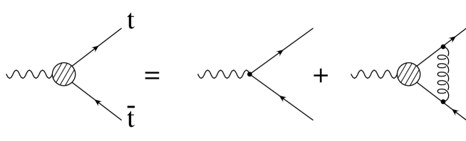
Figure 1: Lippmann–Schwinger equation (1) in diagrammatical form.

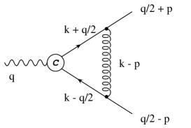
Figure 2: Definition of the four-momenta.

$$\Gamma_{\cal C}={\cal C}+\int{d^{4}k\over(2\pi)^{4}}\left(-{4\over 3}4\pi\alpha_{\rm s}\right)D_{\mu\nu}(p-k)\gamma^{\mu}S_{\rm F}(k+{q\over 2})\Gamma_{\cal C}(k,q)S_{\rm F}(k-{q\over 2})\gamma^{\nu},$$ (1)

with ${\cal C}=\gamma_{\mu}$ or $\gamma_{\mu}\gamma_{5}$ in the cases of interest for $e^{+}e^{-}$-annihilation. The conventions for the flow of momenta are illustrated in Fig. 2. The four-momenta are related to the nonrelativistic variables by

$$q = (2m_{t}+E,{\bf 0})$$

$$p = (0,{\bf p})$$ (2)

$$k = (k_{0},{\bf k}).$$

In perturbation theory the ladder approximation is motivated by the observation that for each additional rung the energy denominator after loop integration compensates the coupling constant attached to the gluon propagator. This is demonstrated most easily in Coulomb gauge. Contributions from transverse gluons as well as those from other diagrams are suppressed by higher powers of $\beta\sim\alpha_{\rm s}$. The gluon propagator is thus replaced by the instantaneous nonrelativistic potential:

$$-{4\over 3}\,4\pi\alpha_{\rm s}D_{\mu\nu}(p)\rightarrow i\,V({\bf p})\,\delta_{\mu 0}\delta_{\nu 0}.$$ (3)

The dominant contribution to the integral originates from the region where $|{\bf k}|\ll m_{t}$. Including terms linear in ${\bf k}$, quark and antiquark propagators are approximated by
$\displaystyle\hskip 43.05542ptS_{\rm F}(k+{q\over 2})$ $\displaystyle=$ $\displaystyle i{\Lambda_{+}-{{\bf k}\cdot\mbox{\boldmath\scriptsize$\gamma$}\over 2m_{t}}\over{E\over 2}+k_{0}-{{\bf k}^{2}\over 2m_{t}}+i{\Gamma_{t}\over 2}}$ $\displaystyle S_{\rm F}(k-{q\over 2})$ $\displaystyle=$ $\displaystyle i{\Lambda_{-}-{{\bf k}\cdot\mbox{\boldmath\scriptsize$\gamma$}\over 2m_{t}}\over{E\over 2}-k_{0}-{{\bf k}^{2}\over 2m_{t}}+i{\Gamma_{t}\over 2}}\,,$ $\displaystyle\Lambda_{\pm}$ $\displaystyle=$ $\displaystyle{1\pm\gamma^{0}\over 2}\,.$ The “elementary” vertex ${\cal C}$ is independent of $k_{0}$. (Within the present approximations this is even true if ${\cal C}$ does depend on ${\bf k}$ as is the case in the analogous treatment of $\gamma\gamma\to t\bar{t}$ discussed below.) Up to and including order $\beta$ terms a self-consistent solution of the integral equation (1) can be obtained if $\Gamma_{\cal C}$ is taken independent of $k_{0}$ and the nonrelativistic spins of $t$ and $\bar{t}$. The $k_{0}$ integration is then easily performed and the integral equation simplified to

$$\Gamma_{\cal C}={\cal C}-\int{d^{3}k\over(2\pi)^{3}}V({\bf p}-{\bf k})\gamma^{0}(\Lambda_{+}-{{\bf k}\cdot\gamma\gamma\gamma\over 2m_{t}}){\Gamma_{\cal C}({\bf k},E)\over E-{{\bf k}^{2}\over m_{t}}+i\Gamma_{t}}(\Lambda_{-}-{{\bf k}\cdot\gamma\gamma\gamma\over 2m_{t}})\gamma^{0}.$$ (5)

In the calculation of the cross section for the production of $t$ plus $\bar{t}$ with momenta $q/2\pm p$ and spins $s_{\pm}$ respectively traces ${\cal H}$ of the following structure will arise:

$${\cal H} = {\rm Tr}\{{\cal P}_{+}({q\over 2}+p,s_{+})\Gamma_{\cal C}{\cal P}_{-}({q\over 2}-p,s_{-})\bar{\Gamma}_{{\cal C}^{\prime}}\},$$ (6)

$${\cal P}_{\pm}(p,s) = {\mbox{$p/$}\pm m_{t}\over 2m_{t}}\,{1+\gamma_{5}\mbox{$s/$}\over 2},$$ (7)

where we allowed for mixed terms with ${\cal C}$ different from ${\cal C}^{\prime}$ arising e.g. from vector-axialvector interference. Expanding again up to terms linear in ${\bf k}$, this trace can be transformed into

$${\cal H} = {\rm Tr}\{{\cal S}_{+}\widetilde{\Gamma}_{\cal C}{\cal S}_{-}\bar{\widetilde{\Gamma}}_{{\cal C}^{\prime}}\},$$ (8)

$${\cal S}_{\pm} = {1\pm{\bf s}_{\pm}\cdot\mbox{\boldmath$\Sigma$}\over 2},$$ (9)

$$\Sigma = \gamma\gamma\gamma\gamma_{5}\gamma^{0}=\left(\begin{array}[]{cc}\mbox{\boldmath$\sigma$}&0\\ 0&\mbox{\boldmath$\sigma$}\end{array}\right),$$ (12)

with the nonrelativistic reduction defined through

$$\widetilde{\Gamma}_{\cal C}({\bf p},E)=\Lambda_{+}\,(1-{{\bf p}\cdot\gamma\gamma\gamma\over 2m_{t}})\,\Gamma_{\cal C}({\bf p},E)\,(1-{{\bf p}\cdot\gamma\gamma\gamma\over 2m_{t}})\,\Lambda_{-}.$$ (13)

It is thus sufficient to calculate the “reduced” vertex function $\widetilde{\Gamma}_{\cal C}$. Dropping again terms of order ${\bf k}^{2}$, the corresponding integral equation is cast into a particularly simple form

$$\widetilde{\Gamma}_{\cal C}({\bf p},E)=\widetilde{{\cal C}}({\bf p})+\int{d^{3}k\over(2\pi)^{3}}V({\bf p}-{\bf k}){\widetilde{\Gamma}_{\cal C}({\bf k},E)\over E-{{\bf k}^{2}\over m_{t}}+i\Gamma_{t}},$$ (14)

where $\widetilde{{\cal C}}({\bf p})$ is defined in analogy to $\widetilde{\Gamma}_{\cal C}({\bf p},E)$ in (13). Consistent with the nonrelativistic approximation only the constant and the linear term in the Taylor expansion of the elementary vertex will be considered

$$\widetilde{{\cal C}}({\bf p})=\widetilde{{\cal C}}(0)+{\bf D}\cdot{\bf p}.$$ (15)

The matrices $\widetilde{\cal C}(0)$ and ${\bf D}$ may in general depend on external momenta, polarization vectors or Lorentz indices. A self-consistent solution for the vertex $\widetilde{\Gamma}_{\cal C}$ is then given by

$$\widetilde{\Gamma}_{\cal C}({\bf p},E)=\widetilde{\cal C}(0){\cal K}_{\rm S}({\rm p},E)+{\bf D}\cdot{\bf p}\,{\cal K}_{\rm P}({\rm p},E).$$ (16)

The scalar vertex functions ${\cal K}_{\rm S,P}$ depend on the modulus of the three momentum

$${\rm p}=|{\bf p}|$$

(which should be distinguished from the four-momentum $p$) and the nonrelativistic energy $E$ only. They are solutions of the nonrelativistic integral equations

$${\cal K}_{\rm S}({\rm p},E) = 1+\int{d^{3}k\over(2\pi)^{3}}V({\bf p}-{\bf k}){{\cal K}_{\rm S}({\rm k},E)\over E-{{\bf k}^{2}\over m_{t}}+i\Gamma_{t}}$$ (17)

$${\cal K}_{\rm P}({\rm p},E) = 1+\int{d^{3}k\over(2\pi)^{3}}{{\bf p}\cdot{\bf k}\over{\bf p}^{2}}V({\bf p}-{\bf k}){{\cal K}_{\rm P}({\rm k},E)\over E-{{\bf k}^{2}\over m_{t}}+i\Gamma_{t}}$$ (18)

and are closely related to the Green function ${\cal G}({\bf p},{\bf x},E)$ which, in turn, is a solution of the Lippmann–Schwinger equation

$$\bigg{[}E-{{\bf p}^{2}\over m_{t}}+i\Gamma_{t}\bigg{]}{\cal G}({\bf p},{\bf x},E)=e^{i{\bf p}\cdot{\bf x}}+\int{d^{3}k\over(2\pi)^{3}}V({\bf p}-{\bf k}){\cal G}({\bf k},{\bf x},E).$$ (19)

Let us denote the first two terms of the Taylor series with respect to ${\bf x}$ by $G$ and $F$ respectively:

$${\cal G}({\bf p},{\bf x},E)=G({\rm p},E)+{\bf x}\cdot i{\bf p}\,F({\rm p},E)+\ldots$$

They are solutions of the integral equations

$$G({\rm p},E) = G_{0}({\rm p},E)+G_{0}({\rm p},E)\int{d^{3}k\over(2\pi)^{3}}V({\bf p}-{\bf k})G({\rm k},E)$$ (20)

$$F({\rm p},E) = G_{0}({\rm p},E)+G_{0}({\rm p},E)\int{d^{3}k\over(2\pi)^{3}}{{\bf p}\cdot{\bf k}\over{\bf p}^{2}}V({\bf p}-{\bf k})F({\rm k},E),$$ (21)

with

$$G_{0}({\rm p},E)={1\over E-{{\bf p}^{2}\over m_{t}}+i\Gamma_{t}},$$ (22)

and the relation between Green function and vertex function

$$G({\rm p},E)=G_{0}({\rm p},E){\cal K}_{\rm S}({\rm p},E),\qquad F({\rm p},E)=G_{0}({\rm p},E){\cal K}_{\rm P}({\rm p},E)$$ (23)

is evident. In the case of $e^{+}e^{-}$-annihilation top production proceeds through the space components of the vector and axial vector current. The relevant elementary vertex $\widetilde{\cal C}({\bf p})$ is given by

$$\widetilde{\gamma_{j}}({\bf p}) = \Lambda_{+}\gamma_{j}\Lambda_{-}$$ (24)

$$\widetilde{\gamma_{j}\gamma_{5}}({\bf p}) = \Lambda_{+}({i\over m_{t}})(\mbox{\boldmath$\gamma$}\times{\bf p})_{j}\Lambda_{-}$$ (25)

for vector and axial current respectively. Production of $t\bar{t}$ in $\gamma\gamma$-fusion would lead to an elementary vertex of the form

$$\widetilde{{\cal C}}(0) \propto i(\mbox{\boldmath$\epsilon$}_{1}\times\mbox{\boldmath$\epsilon$}_{2})\cdot{\bf n}_{e^{-}}\Lambda_{+}\gamma_{5}\Lambda_{-}$$ (26)

$${\bf D} \propto {1\over m_{t}}\Lambda_{+}\left[(\mbox{\boldmath$\epsilon$}_{1}\cdot\mbox{\boldmath$\epsilon$}_{2})({\bf n}_{e^{-}}\cdot\gamma\gamma\gamma){\bf n}_{e^{-}}+(\mbox{\boldmath$\epsilon$}_{2}\cdot\gamma\gamma\gamma)\,\mbox{\boldmath$\epsilon$}_{1}+(\mbox{\boldmath$\epsilon$}_{1}\cdot\gamma\gamma\gamma)\,\mbox{\boldmath$\epsilon$}_{2}\right]\Lambda_{-},$$ (27)

with $\mbox{\boldmath$\epsilon$}_{1}$, $\mbox{\boldmath$\epsilon$}_{2}$ the polarization vectors of the photons, and the present formalism applies equally well. This case has been studied in [21].

2.2 Cross sections and distributions

In the nonrelativistic limit (and defining $E_{t}=p^{0}_{t}-m_{t}$) the two particle phase space for the production of a stable $t$- and $\bar{t}$-quark is conveniently written in the form

$$\int d{\rm PS}=\int{d^{4}p_{t}\over(2\pi)^{4}}\int{d^{4}p_{\bar{t}}\over(2\pi)^{4}}(2\pi)^{4}\delta^{(4)}(p_{t}+p_{\bar{t}}-q)\,\cdot$$

$$\mbox{\hskip 30.00005pt}\cdot\,{1\over 2p_{t}^{0}}2\pi\delta(p_{t}^{0}-\sqrt{m_{t}^{2}+{\bf p}_{t}^{2}})\,{1\over 2p_{\bar{t}}^{0}}2\pi\delta(p_{\bar{t}}^{0}-\sqrt{m_{t}^{2}+{\bf p}_{\bar{t}}^{2}})=$$

$$= {1\over 4m_{t}^{2}}\int{dE_{t}\over 2\pi}{dE_{\bar{t}}\over 2\pi}{d^{3}p\over(2\pi)^{3}}2\pi\delta(E_{t}-{{\bf p}^{2}\over 2m_{t}})2\pi\delta(E_{\bar{t}}-{{\bf p}^{2}\over 2m_{t}})2\pi\delta(E-E_{t}-E_{\bar{t}}).$$

The first two delta functions represent the on-shell conditions for top and antitop quarks. In the case of unstable particles they are replaced by Breit–Wigner functions

$$2\pi\delta(E-{{\bf p}^{2}\over 2m_{t}})\rightarrow{\Gamma_{t}\over(E-{{\bf p}^{2}\over 2m_{t}})^{2}+(\Gamma_{t}/2)^{2}}\quad,$$ (29)

see also discussion in Sect. 3.1 . The $dE_{\bar{t}}$ integration is trivial. The $dE_{t}$ integral can be performed explicitly with the help of the residue theorem. For this second step it is essential that the matrix element is independent of $E_{t}$ for fixed $E$, an assumption evidently fulfilled by the amplitude derived above. The phase space integration is thus cast into the following form

$$\int d{\rm PS}={1\over 4m_{t}^{2}}\int{d^{3}p\over(2\pi)^{3}}{2\Gamma_{t}\over(E-{{\bf p}^{2}\over m_{t}})^{2}+\Gamma_{t}^{2}}.$$ (30)

Therefore only the combinations

$$|G_{0}{\cal K}_{\rm S}|^{2} = |G|^{2}$$ (31)

$${\cal K}_{\rm S}G_{0}\,{\cal K}_{\rm P}^{*}G_{0}^{*} = GF^{*}$$ (32)

appear in the calculation of the $S$-wave dominated differential cross sections and the $S$-$P$–wave interference terms.

2.3 Top production in electron positron annihilation

With these ingredients it is straightforward to calculate the differential momentum distribution and the polarization of top quarks produced in electron positron annihilation. Let us introduce the following conventions for the fermion couplings

$$v_{f}=2I^{3}_{f}-4q_{f}\sin^{2}\theta_{\rm W},\qquad a_{f}=2I^{3}_{f}.$$ (33)

$P_{\pm}$ denotes the longitudinal electron/positron polarization and

$$\chi={P_{+}-P_{-}\over 1-P_{+}P_{-}}$$ (34)

can be interpreted as effective longitudinal polarization of the virtual intermediate photon or $Z$ boson. The following abbreviations will be useful below:

$$a_{1} = q_{e}^{2}q_{t}^{2}+(v_{e}^{2}+a_{e}^{2})v_{t}^{2}d^{2}+2q_{e}q_{t}v_{e}v_{t}d$$

$$a_{2} = 2v_{e}a_{e}v_{t}^{2}d^{2}+2q_{e}q_{t}a_{e}v_{t}d$$

$$a_{3} = 4v_{e}a_{e}v_{t}a_{t}d^{2}+2q_{e}q_{t}a_{e}a_{t}d$$ (35)

$$a_{4} = 2(v_{e}^{2}+a_{e}^{2})v_{t}a_{t}d^{2}+2q_{e}q_{t}v_{e}a_{t}d$$

$$d = {1\over 16\sin^{2}\theta_{\rm W}\cos^{2}\theta_{\rm W}}\,{s\over s-M_{Z}^{2}}.$$

The differential cross section, summed over polarizations of quarks and including $S$-wave and $S$-$P$–interference contributions, is thus given by

$${d^{3}\sigma\over dp^{3}} = {3\alpha^{2}\Gamma_{t}\over 4\pi m_{t}^{4}}(1-P_{+}P_{-})\left[{(a_{1}+\chi a_{2})\left(1-{16\alpha_{\rm s}\over 3\pi}\right)\left|G({\rm p},E)\right|^{2}+}\right.$$ (36)

$$\left.{+(a_{3}+\chi a_{4})\left(1-{12\alpha_{\rm s}\over 3\pi}\right){{\rm p}\over m_{t}}{\rm Re}\left(\,G({\rm p},E)F^{*}({\rm p},E)\,\right)\,\cos\vartheta}\right].$$

The vertex corrections from hard gluon exchange for $S$-wave [22] and $P$-wave [24] amplitudes are included in this formula. It leads to the following forward-backward asymmetry

$${\cal A}_{\rm FB}({\rm p},E)=C_{\rm FB}(\chi)\,\varphi_{\rm{}_{R}}({\rm p},E),$$ (37)

with

$$C_{\rm FB}(\chi)={1\over 2}\,{a_{3}+\chi a_{4}\over a_{1}+\chi a_{2}},$$ (38)

$\varphi_{\rm{}_{R}}={\rm Re}\,\varphi$, and

$$\varphi({\rm p},E)={(1-{4\alpha_{\rm s}/3\pi})\over(1-{8\alpha_{\rm s}/3\pi})}\,{{\rm p}\over m_{t}}\,{F^{*}\!({\rm p},E)\over G^{*}\!({\rm p},E)}.$$ (39)

This result is still differential in the top quark momentum. Replacing $\varphi({\rm p},E)$ by

$$\Phi(E)={(1-{4\alpha_{\rm s}/3\pi})\over(1-{8\alpha_{\rm s}/3\pi})}\,{\int_{0}^{{\rm p}_{m}}d{\rm p}\,{{\rm p}^{3}\over m_{t}}\,F^{*}({\rm p},E)G({\rm p},E)\over\int_{0}^{{\rm p}_{m}}d{\rm p}\,{\rm p}^{2}\left|G({\rm p},E)\right|^{2}}.$$ (40)

one obtains the integrated forward-backward asymmetry. The cutoff ${\rm p}_{m}$ must be introduced to eliminate the logarithmic divergence of the integral. For free particles (or sufficiently far above threshold) one finds for example

$$\Phi(E)=\sqrt{\frac{E}{m_{t}}}+\frac{2\Gamma_{t}}{\sqrt{m_{t}E}\pi}\ln{{\rm p}_{m}\over m_{t}}\,.$$ (41)

This logarithmic divergence is a consequence of the fact that the nonrelativistic approximation is used outside its range of validity. One may either choose a cutoff of order $m_{t}$ or replace the nonrelativistic phase space element ${\rm p}\,d{\rm p}/m_{t}$ by ${\rm p}\,d{\rm p}/\sqrt{m_{t}^{2}+{\rm p}^{2}}$. In practical applications a cutoff will be introduced by the experimental procedure used to define $t\bar{t}$-events.

2.4 Polarization

Figure 3: Definition of the spin directions. The normal component ${\bf s}_{\rm N}$ points out of the plane.

To describe top quark production in the threshold region it is convenient to align the reference system with the beam direction (Fig. 3) and to define

$${\bf s}_{\|} = {\bf n}_{e^{-}}$$

$${\bf s}_{\rm N} = {{\bf n}_{e^{-}}\times{\bf n}_{t}\over|{\bf n}_{e^{-}}\times{\bf n}_{t}|}$$ (42)

$${\bf s}_{\bot} = {\bf s}_{\rm N}\times{\bf s}_{\|}.$$

In the limit of small $\beta$ the quark spin is essentially aligned with the beam direction apart from small corrections proportional to $\beta$, which depend on the production angle. A system of reference with ${\bf s}_{\|}$ defined with respect to the top quark momentum [25] is convenient in the high energy limit but evidently becomes less convenient close to threshold.

The differential cross section for production of a top quark of three-momentum ${\bf p}$ and spin projection $+1/2$ on direction ${\bf s}_{+}$ reads

$${d^{3}\sigma({\bf p},{\bf s}_{+})\over dp^{3}}\;=\;{1\over 2}\,\left(1+\mbox{\boldmath$\cal P$}\cdot{\bf s}_{+}\right)\,{d^{3}\sigma\over dp^{3}}\;.$$ (43)

The three-vector $\cal P$ characterizes the polarization of the top quark. Its components ${\cal P}^{i}$ can be obtained from the formula

$${\cal P}^{i}\;=\;\left[\,{d^{3}\sigma({\bf p},{\bf s}_{+}^{(i)})\over dp^{3}}-{d^{3}\sigma({\bf p},{\bf s}_{+}^{(i)})\over dp^{3}}\,\right]\;\left/\;\left[\,{d^{3}\sigma({\bf p},{\bf s}_{+}^{(i)})\over dp^{3}}+{d^{3}\sigma({\bf p},{\bf s}_{+}^{(i)})\over dp^{3}}\,\right]\right.$$ (44)

where ${\bf s}_{+}^{(i)}\;=\;{\bf s}_{{}_{\|}},\;{\bf s}_{\bot}$ and ${\bf s}_{\rm N}$. Including the QCD potential one obtains for the three components of the polarization

$${\cal P}_{\|}({\bf p},E,\chi) = C_{\|}^{0}(\chi)+C_{\|}^{1}(\chi)\,\varphi_{\rm{}_{R}}({\rm p},E)\,\cos\vartheta\,$$ (45)

$${\cal P}_{\bot}({\bf p},E,\chi) = C_{\bot}(\chi)\,\varphi_{\rm{}_{R}}({\rm p},E)\,\sin\vartheta\,$$ (46)

$${\cal P}_{\rm N}({\bf p},E,\chi) = C_{\rm N}(\chi)\varphi_{\rm{}_{I}}({\rm p},E)\sin\vartheta\,,$$ (47)

$$\hskip 21.52771ptC_{\|}^{0}(\chi)=-{a_{2}+\chi a_{1}\over a_{1}+\chi a_{2}},\hskip 29.7082ptC_{\|}^{1}(\chi)=\left(1-\chi^{2}\right){a_{2}a_{3}-a_{1}a_{4}\over\left(a_{1}+\chi a_{2}\right)^{2}},$$

$$\hskip 21.52771ptC_{\bot}(\chi)=-{1\over 2}\,{a_{4}+\chi a_{3}\over a_{1}+\chi a_{2}},\qquad C_{\rm N}(\chi)=-{1\over 2}\,{a_{3}+\chi a_{4}\over a_{1}+\chi a_{2}}\,=\,-C_{\rm FB}(\chi),$$

with $\varphi_{\rm{}_{I}}={\rm Im}\,\varphi$, and $\varphi({\rm p},E)$ as defined in (39). The momentum integrated quantities are obtained by the replacement $\varphi({\rm p},E)\to\Phi(E)$. The case of non-interacting stable quarks is recovered by the replacement $\Phi\to\beta$, an obvious consequence of (40).

Let us emphasize the main qualitative features of the result:

• Top quarks in the threshold region are highly polarized. Even for unpolarized beams the longitudinal polarization amounts to about $-0.41$ and reaches $\pm 1$ for fully polarized electron beams. This later feature is of purely kinematical origin and independent of the structure of top quark couplings. Precision studies of polarized top decays are therefore feasible.

• Corrections to this idealized picture arise from the small admixture of $P$-waves. The transverse and the normal components of the polarization are of order 10%. The angular dependent part of the parallel polarization is even more suppressed. Moreover, as a consequence of the angular dependence its contribution vanishes upon angular integration.

• The QCD dynamics is solely contained in the functions $\varphi$ or $\Phi$ which is the same for the angular distribution and the various components of the polarization. (However, this “universality” is affected by the rescattering corrections as discussed in Sect. 3.) These functions which evidently depend on QCD dynamics can thus be studied in a variety of ways.

• The relative importance of $P$-waves increases with energy, $\Phi\sim\sqrt{E/m_{t}}$. This is expected from the close analogy between $\Phi_{\rm R}={\rm Re}\,\Phi$ and $\beta$. In fact, the order of magnitude of the various components of the polarization above, but close to threshold, can be estimated by replacing $\Phi_{\rm R}\to{\rm p}/m_{t}$.

The $C_{i}$ are displayed in Fig. 4 as functions of the variable $\chi$. For the weak mixing angle a value $\sin^{2}\!\theta_{\rm W}=0.2317$ is adopted, for the top mass $m_{t}=180$ GeV. As discussed before, $C_{\|}^{0}$ assumes its maximal value $\pm 1$ for $\chi=\mp 1$ and the coefficient $C_{\|}^{1}$ is small throughout. The coefficient $C_{\bot}$ varies between $+0.7$ and $-0.5$ whereas $C_{\rm N}$ is typically around $-0.5$. The dynamical factors $\Phi$ are around $0.1$ or larger, such that the $P$-wave induced effects should be observable experimentally.

Figure 4: The coefficients (LABEL:coefs) for $\sqrt{s}/2=m_{t}=180$ GeV.

The normal component of the polarization which is proportional to $\varphi_{\rm{}_{I}}$ has been predicted for stable quarks in the framework of perturbative QCD [26, 25]. In the threshold region the phase can be traced to the $t\bar{t}$ rescattering by the QCD potential. For stable quarks, assuming a pure Coulomb potential $V=-4\alpha_{\rm s}/3r$, the nonrelativistic problem can be solved analytically [21] and one finds

$$\lim_{\Gamma_{t}\rightarrow 0\atop E\rightarrow{\bf p}^{2}/m_{t}}\left(E-{{\bf p}^{2}\over m_{t}}+i\Gamma_{t}\right)G({\rm p},E) = \exp\left(\pi{\bar{k}}\over 2{\rm p}\right)\,\Gamma(1+{i{\bar{k}}/{\rm p}})$$ (49)

$$\lim_{\Gamma_{t}\rightarrow 0\atop E\rightarrow{\bf p}^{2}/m_{t}}\left(E-{{\bf p}^{2}\over m_{t}}+i\Gamma_{t}\right)F({\rm p},E) = \left(1-i{{\bar{k}}\over{\rm p}}\right)\exp\left(\pi{\bar{k}}\over 2{\rm p}\right)\,\Gamma(1+{i{\bar{k}}/{\rm p}}),\ \ \ \ \$$ (50)

with ${\bar{k}}=2m_{t}\alpha_{s}/3$ and hence

$$\varphi_{\rm{}_{I}}({\rm p},E) \rightarrow {2\over 3}\alpha_{\rm s}{1-4\alpha_{\rm s}/3\pi\over 1-8\alpha_{\rm s}/3\pi}$$ (51)

$$\Phi_{\rm I}({\rm p},E) \rightarrow {2\over 3}\alpha_{\rm s}{1-4\alpha_{\rm s}/3\pi\over 1-8\alpha_{\rm s}/3\pi}.$$ (52)

The component of the polarization normal to the production plane is thus approximately independent of $E$ and essentially measures the strong coupling constant. In fact one can argue that this is a unique way to get a handle on the scattering of heavy quarks through the QCD potential.

3 Rescattering corrections to the differential cross section

3.1 Introductory remarks

Close to threshold, the velocity $\beta$ of the top quark is of the same order of magnitude as the strong coupling. To include only the ${\cal O}(\beta)$ contributions to the differential cross section and polarization and discard rescattering corrections is thus inconsistent. To obtain reliable predictions for the observables it is mandatory to calculate the ${\cal O}(\alpha_{\rm s})$ corrections. Some of these can be implemented without much effort as they are known since several years, and in fact they have already been taken into account in the preceding formulæ:

• the modification of the $t\bar{t}V$ and $t\bar{t}A$ vertices due to transverse gluon exchange for small $\beta$ simply reduces to a multiplication by constant form factors [30]:

  $$G({\rm p},E) \longrightarrow \Big{(}1-\frac{8\alpha_{\rm s}}{3\pi}\Big{)}G({\rm p},E)$$ (53)

  $$F({\rm p},E) \longrightarrow \Big{(}1-\frac{4\alpha_{\rm s}}{3\pi}\Big{)}F({\rm p},E).$$ (54)

  This explains the corresponding factors in (36) and in the definition of $\varphi({\bf p},E)$ and $\Phi(E)$ (39).

• Corrections to $t$ or $\bar{t}$ decay can be taken into account by using the full 1-loop result for $\Gamma_{t}$ [17].

If the total cross section were the only quantity of interest, all next-to-leading contributions would be included this way, because it is well known since quite some time that the excitation curve is free of (other) ${\cal O}(\alpha_{\rm s})$ corrections [31]. This result has also been re-established recently [14, 15]. But this statement does not hold for the differential cross section or polarization, since these are affected through the diagrams shown in Figs. 5a and 5b (and a third diagram with gluon exchange between the two $b$-quarks, which can, however, be neglected), i.e. corrections caused by interactions between the decay products of one of the top quarks with the second top. They will also be called rescattering corrections.

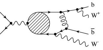
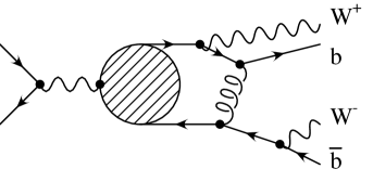
a)	b)

Figure 5: Lowest order rescattering diagrams.

Their calculation obviously requires a modification of the approach as at least the decay of one of the two top (anti)quarks has to be included. In this section a formalism will be pursued which attempts to retain the notion of quark polarization in the presence of rescattering of decay products. In Sect. 4 a slightly different strategy will be adopted which aims directly at predictions for experimentally observable lepton distributions, viz. appropriately chosen moments. Let us start with the first approach and write the differential cross section in the following form :

$$\frac{d^{3}\sigma(\bf p,s_{+})}{dp^{3}} = \frac{3\alpha^{2}}{64m_{t}^{6}}\frac{1-P_{e^{+}}P_{e^{-}}}{4\pi}\sum_{i,j=1,2}(a_{1}+a_{2}\chi)\Big{(}L_{s}^{ij}+C_{\parallel}^{0}L_{a}^{ij}\Big{)}H^{VV}_{ij}$$ (55)

$$+{\cal O}(\beta)\mbox{ terms}.$$

The three-vector ${\bf s_{+}}$ describes the spin of top quark, which in this subsection is considered as a well defined quantity. The leptonic tensors $L^{ij}$ are defined through

$$L_{s}^{ij}=8m_{t}^{2}\delta^{ij}~{},~{}L_{a}^{ij}=-8m_{t}^{2}i\epsilon^{ij}~{},~{}i,j=1..2~{}.$$ (56)

As already discussed in the preceding section the terms of order $\beta$ arise from $S$-$P$–wave interference, i.e. from interference between the amplitudes corresponding to vector and axialvector couplings $t\bar{t}\gamma$ and $t\bar{t}Z^{0}$. In the approximation of the present article contributions suppressed by $\alpha_{s}\beta$ are neglected. Hence it suffices to consider order $\alpha_{s}$ corrections to contributions involving only vector couplings and the corresponding vertex functions ${\cal K}_{\rm S}({\rm p},E)$. $H^{VV}_{ij}$ represents the leading (vector-vector) part of the hadronic tensor

$$H^{VV}_{ij}=\int\!\frac{dp_{0}}{2\pi}\int\!d\mbox{PS}_{2}(t;bW^{+})\int\!d\mbox{PS}_{2}(\bar{t};\bar{b}W^{-})\,\sum_{\epsilon_{\pm}}\,{\cal M}_{i}{\cal M}_{j}^{\dagger}~{}+~{}\mbox{c.c.}$$ (57)

where ${\cal M}_{i}$ denotes the amplitude for $V\to t\bar{t}\to b\bar{b}W^{+}W^{-}$. The momenta of top and antitop are given by $t=b+W^{+}=q/2+p$, $\bar{t}=\bar{b}+W^{-}=q/2-p$ and ${\epsilon_{\pm}}$ denote the polarization vectors of $W^{\pm}$.

This approach can be adopted in a straightforward way as long as only factorizable diagrams are considered where the top quark decay products do not rescatter. Diagram Fig. 5b, however, as a truly non-factorizable contribution leads to difficulties when discussing the top quark polarization as will become clear below. Nevertheless this formalism will be presented for pedagogical reasons before a more powerful approach will be introduced in Sect. 4.

To lowest order in the nonrelativistic approximation the amplitude ${\cal M}_{i}$ is given by

$${\cal M}^{(0)}_{i}({\bf s}_{+}) = -\Big{(}\frac{ig_{w}}{\sqrt{8}}\Big{)}^{2}\bar{u}(b)\not\!\epsilon_{+}(1-\gamma^{5})\frac{1+\gamma_{5}\!\not\!s_{+}}{2}\Lambda_{+}\gamma_{i}\Lambda_{-}\not\!\epsilon_{-}(1-\gamma^{5})v(\bar{b})$$ (58)

$$\cdot G({\rm p},E)\Big{(}G_{t}(p,E)+G_{\bar{t}}(p,E)\Big{)}$$

with the nonrelativistic propagators introduced in (4) (see also App. A),

$$S_{\rm F}(p\pm\frac{q}{2})=i\Big{(}\Lambda_{\pm}-\frac{\bf p\cdot\mbox{\boldmath$\gamma$}}{2m}\Big{)}\cdot G_{t/\bar{t}}(p,E),$$

and where

$$-S_{\rm F}(p+q/2)\widetilde{\Gamma}^{i}_{V}S_{\rm F}(p-q/2) \approx \Lambda_{+}\gamma^{i}\Lambda_{-}{\cal K}_{\rm S}({\rm p},E)G_{t}(p,E)G_{\bar{t}}(p,E)$$ (59)

$$= \Lambda_{+}\gamma^{i}\Lambda_{-}G({\rm p},E)(G_{t}(p,E)+G_{\bar{t}}(p,E))$$

has been used. The amplitude ${\cal M}^{(0)}_{i}(s_{+})$ depends on $s_{+}$ which for a stable top quark would be interpreted as its polarization four-vector. For unstable top quark this interpretation is still valid if the decay products do not interact. In such a case the total angular momentum of the $W^{+}b$ subsystem is conserved. Thus, in principle at least, the angular momentum state $|{1\over 2},m\rangle$ of $W^{+}b$ can be inferred from the measurement of the spin-dependent angular distributions of $W$ and $b$. The quantum number $m$ denotes an eigenvalue of the angular momentum projection on direction $\bf s_{+}$. It is evident that one can identify $m$ with the projection of top quark spin if there is no interaction changing momenta and polarizations of $W$ and $b$ after the decay.

Inserting the expression for ${\cal M}$ into (55) and (57), summing over polarizations $\epsilon_{+}$ and $\epsilon_{-}$, and performing the $(bW^{+})$ and $(\bar{b}W^{-})$ phase space integrations with the help of

$$\frac{g_{w}^{2}}{4}\int\!d\mbox{PS}_{2}(t;bW^{+})\sum_{\epsilon_{+}}\not\!\epsilon_{+}\not\!b\not\!\epsilon_{+}(1-\gamma^{5})=\frac{\Gamma_{t}}{m_{t}}\not\!t(1-\gamma^{5})$$ (60)

and the corresponding identity for the $(\bar{b}W^{-})$ system, one re-derives the results given in the preceding section. The inclusion of the axialvector couplings and calculation of the $S$-$P$–wave interference effects can be done in an analogous way.

3.2 Rescattering in the $t\bar{b}$ system

The rescattering in the $t\bar{b}$ system is given by diagram 5a and leads to an additional amplitude of the form

$${\cal M}^{a}_{i} = \Big{(}\frac{ig_{w}}{\sqrt{8}}\Big{)}^{2}\int\!\frac{d^{4}k}{(2\pi)^{4}}\bar{u}(b)\not\!\epsilon_{+}(1\!-\gamma^{5})i\Lambda_{+}\gamma^{\mu}\Lambda_{+}\gamma_{i}\Lambda_{-}\!\not\!\epsilon_{-}(1-\gamma^{5})S_{\rm F}(k\!-\!p\!-\!\bar{b})$$ (61)

$$\gamma^{\nu}v(\bar{b})\cdot G_{t}(p,E)G({\rm k},E)\Big{(}G_{t}(k,E)+G_{\bar{t}}(k,E)\Big{)}D_{\mu\nu}(k-p)g_{s}^{2}C_{F}\quad.$$

In this amplitude all the top quark propagators have been substituted by their nonrelativistic limits

$$S_{\rm F}(t)\longrightarrow i\Lambda_{+}G_{t}(p,E).$$

As a consequence the top quark couples to gluons via the projection $\Lambda_{+}\gamma^{\mu}\Lambda_{+}$, which implies that only instantenous Coulomb-like gluon exchange contributes to leading order. In the calculation of the ${\cal O}(\alpha_{\rm s})$ corrections to the differential cross sections

$$\sim\;\int\!\frac{dp_{0}}{2\pi}\int\!d\mbox{PS}_{2}(t;bW^{+})\int\!d\mbox{PS}_{2}(\bar{t};\bar{b}W^{-})\,\sum_{\epsilon_{+},\epsilon_{-}}\,\Big{(}{\cal M}^{(0)}_{i}(s_{+}){\cal M}^{(a)\dagger}_{j}+{\cal M}^{(a)}_{i}{\cal M}^{(0)\dagger}_{j}(s_{+})\Big{)}$$

only the interference of ${\cal M}^{a}_{i}$ with the lowest order amplitude ${\cal M}^{(0)}_{i}(s_{+})$ contributes. A more detailed description of the calculation of this contribution is presented in App. A. At this point it should suffice to mention that it essentially involves choosing the appropriate integration contours and using the residue theorem. The result can be written in the following compact form:

$$\frac{d\sigma^{(a)}}{d{\rm p}d\Omega}=\frac{1}{4\pi}\frac{d\sigma^{(0)}}{d{\rm p}}\frac{1}{4}\Big{(}\psi_{1}({{\rm p}},E)+C^{0}_{\parallel}\,\kappa\,\psi_{\rm{}_{R}}({\rm p},E)\cos\vartheta+{\bf P\cdot s}_{+}\Big{)},$$ (62)

where $d\sigma^{(0)}/d{\rm p}$ denotes the top quark momentum distribution in the lowest order approximation,

$$P_{\parallel} = C_{\parallel}^{0}\,\psi_{1}({\rm p},E)+\kappa\,\psi_{\rm{}_{R}}({\rm p},E)\cos\vartheta~{},$$ (63)

$$P_{\perp} = P_{\rm N}=0~{},$$ (64)

$$\kappa = \frac{1-2y}{1+2y}\qquad\mbox{and}\qquad y=\frac{m_{W}^{2}}{m_{t}^{2}}.$$ (65)

The two functions $\psi_{1}$ and $\psi_{\rm{}_{R}}$ are defined as the following convolutions:

$$\psi_{1}({\rm p},E) = 2\,{\rm Im}\int\!\frac{d^{3}k}{(2\pi)^{3}}V(|{\bf k}-{\bf p}|)\frac{G({\rm k},E)}{G({\rm p},E)}\frac{\arctan{\frac{|{\bf k}-{\bf p}|}{\Gamma_{t}}}}{|{\bf k}-{\bf p}|}$$ (66)

$$\psi_{2}({\rm p},E) = 2\int\!\frac{d^{3}k}{(2\pi)^{3}}V(|{\bf k}-{\bf p}|)\frac{{\bf p}\cdot({\bf k-p})}{|{\bf p}||{\bf k-p}|^{2}}\frac{G({\rm k},E)}{G({\rm p},E)}$$ (67)

$$\times\Big{(}1-\frac{\Gamma_{t}}{|{\bf k}-{\bf p}|}\arctan{\frac{|{\bf k}-{\bf p}|}{\Gamma_{t}}}\Big{)}$$

$$\psi_{\rm{}_{R}}({\rm p},E) = {\rm Re}\;\psi_{2}({\rm p},E).$$ (68)

It is noteworthy that rescattering in the $t\bar{b}$ system does not affect the transverse and normal components of the top quark polarization. The top quark width $\Gamma_{t}$ acts as an infrared cutoff: in the limit $\Gamma_{t}\to 0$ the real part of $\psi_{2}$ becomes infrared divergent.

3.3 Rescattering in the $(Wb)\bar{t}$ system

The corrections due to rescattering of the top quark decay products on the spectator $\bar{t}$ can be calculated in an analogous way. They result from the interference of diagram 5b and the lowest order amplitude ${\cal M}^{(0)}_{i}(s_{+})$. However, for diagram 5b it is not possible to identify the total angular momentum $j$ of the $W^{+}b$ system and the spin of the top quark. In fact the latter quantity is not well defined and $j$ can be different from $1/2$. However, only for $j=1/2$ and $m=\pm 1/2$ there are non-zero contributions to order $\alpha_{s}$ corrections

$$\sim\;\int\!\frac{dp_{0}}{2\pi}\int\!d\mbox{PS}_{2}(t;bW^{+})\int\!d\mbox{PS}_{2}(\bar{t};\bar{b}W^{-})\,\sum_{\epsilon_{+},\epsilon_{-}}\,\Big{(}{\cal M}^{(0)}_{i}(s_{+}){\cal M}^{(b)\dagger}_{j}+{\cal M}^{(b)}_{i}{\cal M}^{(0)\dagger}_{j}(s_{+})\Big{)}.$$

Summing over $W^{\pm}$ polarizations and calculating the phase space integrals one obtains

$$\frac{d\sigma^{(b)}}{d{\rm p}d\Omega}=\frac{1}{4\pi}\frac{d\sigma^{(0)}}{d{\rm p}}\frac{1}{4}\Big{(}\psi_{1}({\rm p},E)+C^{0}_{\parallel}\,\kappa\,\psi_{\rm{}_{R}}({\rm p},E)\cos\vartheta+{\bf P\cdot s}_{+}\Big{)}$$ (69)

with

$$P_{\parallel} = C_{\parallel}^{0}\,\psi_{1}({\rm p},E)+\kappa\,\psi_{\rm{}_{R}}({\rm p},E)\cos\vartheta$$ (70)

$$P_{\perp} = \kappa\,\psi_{\rm{}_{R}}({\rm p},E)\sin\vartheta$$ (71)

$$P_{\rm N} = C^{0}_{\parallel}\,\kappa\,\psi_{\rm{}_{I}}({\rm p},E)\sin\vartheta$$ (72)

where the additional function

$$\psi_{\rm{}_{I}}({\rm p},E)={\rm Im}\,\psi_{2}({\rm p},E)$$ (73)

appears.

At first glance this result may be surprising. One might have thought that any interaction after top decay cannot influence top polarization. There is however a problem with such a simple picture, because the spin of an intermediate (virtual) particle is not a well defined quantity and thus no observable. What has been calculated by using the spin projection operator should be interpreted as the $(bW)$ total angular momentum, which coincides with top spin on Born level only. Clearly the angular momentum of $Wb$ may well be influenced by final state interactions. From a practical point of view it will be quite difficult if not impossible to measure this quantity.

It definitely makes more sense to consider the angular distribution of the charged leptons from the decay $t\to W^{+}b\to l^{+}\nu_{l}b$ instead. Rescattering in the $(Wb)\bar{t}$ system produces a contribution which is non-factorizable, i.e. it is impossible to write the final expression in the form

$$\frac{d^{6}\sigma(e^{+}e^{-}\to l^{+}\nu_{l}bW^{-}\bar{b})}{dp^{3}dE_{l}d\Omega_{l}}=\frac{d^{3}\sigma(e^{+}e^{-}\to t\bar{t})}{dp^{3}}\frac{1}{\Gamma_{t}}\frac{d\Gamma_{t\to bl\nu}({\bf s}_{+})}{dE_{l}d\Omega_{l}}$$ (74)

which is possible for all the other diagrams.

3.4 Momentum distribution and polarizations

Adding the contributions discussed in the preceding subsections one can calculate the order $\alpha_{s}$ correction to the differential cross section summed over spins. The momentum distribution is affected by $\psi_{1}$ only:

$$\frac{d\sigma^{(0)}}{d{\rm p}}\to\frac{d\sigma^{(1)}}{d\rm p}=\frac{d\sigma^{(0)}}{d\rm p}\cdot\Big{(}1+\psi_{1}({\rm p},E)\Big{)}.$$ (75)

It follows that at order $\alpha_{s}$ the total cross section for $t\bar{t}$ production is unaffected by rescattering corrections[14, 15]. Indeed

$$\int\!\frac{d^{3}p}{(2\pi)^{3}}|G({\rm p},E)|^{2}\psi_{1}({\rm p},E)=0$$ (76)

because for any real function $f(|{\bf k}-{\bf p}|)$ the integral

$$J=\int\!\frac{d^{3}p}{(2\pi)^{3}}\int\!\frac{d^{3}k}{(2\pi)^{3}}G({{\rm p}},E)G^{*}({{\rm k}},E)f(|{\bf k}-{\bf p}|)=J^{*}$$

is real.

The function $\psi_{2}({{\rm p}},E)$ gives the order $\alpha_{s}$ corrections to the forward-backward asymmetry ${\cal A}_{\rm FB}$ and the polarization vector $\cal P$ of the $bW$ system. It is interesting to note similarities between these formulæ and the ${\cal O}(\beta)$ expressions:

$${\cal A}_{\rm FB}^{{}^{\rm resc}}({\rm p},E) = \frac{C_{\parallel}^{0}}{2}\kappa\,\psi_{\rm{}_{R}}({\rm p},E)$$ (77)

$${\cal P}_{\parallel}^{{}^{\rm resc}}({\rm p},E) = \Big{(}1-(C_{\parallel}^{0})^{2}\Big{)}\kappa\,\psi_{\rm{}_{R}}({\rm p},E)\cos\vartheta$$ (78)

$${\cal P}_{\perp}^{{}^{\rm resc}}({\rm p},E) = \frac{1}{2}\kappa\,\psi_{\rm{}_{R}}({\rm p},E)\sin\vartheta$$ (79)

$${\cal P}_{\rm N}^{{}^{\rm resc}}({\rm p},E) = \frac{C_{\parallel}^{0}}{2}\kappa\,\psi_{\rm{}_{I}}({\rm p},E)\sin\vartheta.$$ (80)

Let us close this section with two remarks. The results for the unpolarized case have been first derived in [15] and are in accordance with ours. Following [15, 16] one can consider also the diagram with gluon exchange between $b$ and $\bar{b}$. However, it has already been argued in the Introduction that this contribution is suppressed. Our conclusion is supported by the results of [15, 16] for unpolarized beams.

4 Moments of the lepton spectrum

It has already been stated that the optimal way to experimentally determine top quark polarization is based on the analysis of the charged lepton distribution in the process

$$e^{+}e^{-}\to t\bar{t}\to bl\nu\bar{b}W^{-}.$$

A particularly convenient distribution is the charged lepton angular distribution, which for free top quark decay in its rest frame is given by the formula

$$\frac{d\Gamma}{d\Omega_{l}}=\frac{\Gamma}{4\pi}\Big{(}1+|{\mbox{\boldmath$\cal P$}}|\cos\theta\Big{)}$$ (81)

where $\theta$ denotes the angle between the lepton momentum and top polarization $\cal P$. It is quite straightforward to generalize this formula to the case of factorizable contributions to $t\bar{t}$ production, c.f. (74). In fact this problem can be solved by using the Lorentz transformation from the top quark rest frame to the center-of-mass frame for the $t\bar{t}$ system. However the diagram of Fig.5b leads to a non-factorizable contribution with production and decay mechanisms coupled in an intricate way. The corresponding expression for the angular distribution of the charged lepton involves a complicated integral over the phase space and the three-momentum transfer between $b$ and $\bar{t}$. In particular integration over the phase space of the top quark is difficult because the direction of the charged lepton in $t\to bW\to bl\nu$ is fixed and one cannot use Lorentz symmetry to perform integrations. We were unable to simplify this expression. It is more convenient to consider moments of the charged lepton distribution which are given by manifestly Lorentz invariant integrals over the three-body Lorentz invariant phase space ${\rm PS}_{3}(t;bl\nu)$. Moreover, these moments are measurable and contain important information on polarization. From the calculational point of view Lorentz symmetry simplifies the problem considerably and closed expressions can be derived even for non-factorizable contributions.

Let $l$ be the four-momentum of the charged lepton and $n$ denote one of the following four-vectors, which in the $t\bar{t}$ rest frame read, c.f. (42):

$$n_{\|} = \left(0,{\bf s}_{\|}\,\right)$$ (82)

$$n_{\bot} = \left(0,{\bf s}_{\bot}\,\right)$$ (83)

$$n_{\rm N} = \left(0,{\bf s}_{\rm N}\right)$$ (84)

$$n_{(0)} = (1,0,0,0)$$ (85)

The moments are defined as the average values of the scalar products $(nl)$. One can consider the moments $\langle nl\rangle$ for a fixed three-momentum of the top quark,

$$\langle nl\rangle\equiv\Big{(}\frac{d^{3}\sigma}{d{\rm p}d\Omega_{p}}\Big{)}^{-1}\int dE_{l}d\Omega_{l}\frac{d\sigma(e^{+}e^{-}\to bl\nu\bar{b}W^{-})}{d{\rm p}d\Omega_{p}d\Omega_{l}dE_{l}}(nl)$$ (86)

or, integrating over the direction of the top quark, the moments

$$\langle\langle nl\rangle\rangle\equiv\Big{(}\frac{d\sigma}{d{\rm p}}\Big{)}^{-1}\int dE_{l}d\Omega_{l}d\Omega_{p}\frac{d\sigma(e^{+}e^{-}\to bl\nu\bar{b}W^{-})}{d{\rm p}d\Omega_{p}d\Omega_{l}dE_{l}}(nl)$$ (87)

or, finally the moments $\langle\langle\langle nl\rangle\rangle\rangle$ integrated also over ${\rm p}$. The calculation of these quantities is straightforward because the integral over the three-body phase space $\mbox{PS}_{3}(t;bl\nu)$ can be calculated analytically. The hadronic tensor for the differential cross section is given by

$$H_{ij}=\int\!\frac{dp_{0}}{2\pi}\int\frac{dW^{2}}{2\pi}\int d\mbox{PS}_{3}(t;bl\nu)\int d\mbox{PS}_{2}(\bar{t};\bar{b}W^{-})\,\sum_{\epsilon_{-}}{\cal M}_{i}{\cal M}_{j}^{\dagger}$$ (88)

with the appropriate amplitudes including semileptonic $W^{+}$ decays. The corresponding tensor needed for the determination of the moments will be called $H_{ij;n}$ and simply contains the additional factor $(nl)$ under the integrals

$$H_{ij;n}=\int\!\frac{dp_{0}}{2\pi}\int\frac{dW^{2}}{2\pi}\int d\mbox{PS}_{3}(t;bl\nu)\int d\mbox{PS}_{2}(\bar{t};\bar{b}W^{-})\,\sum_{\epsilon_{-}}{\cal M}_{i}{\cal M}_{j}^{\dagger}\,(nl)$$ (89)

Using the following decomposition of the three-body phase space

$$\int d\mbox{PS}_{3}(t;bl\nu)=\frac{1}{2\pi}\int dW^{2}\int d\mbox{PS}_{2}(t;bW)\int d\mbox{PS}_{2}(W;l\nu)$$ (90)

one can reduce the calculation to a sequence of Lorentz invariant integrations over two-body phase spaces. A more detailed description of the calculation can be found in App. B.

Let us, for illustrative purpose, discuss the Born- and $S$-$P$–wave interference part. In this case one arrives at

$$\langle nl\rangle=\mbox{BR}(t\to bl\nu)\frac{1+2y+3y^{2}}{4(1+2y)}\Big{[}(tn)+\frac{m_{t}}{3}(n{\cal P})\Big{]}$$ (91)

with $y$ (and $\kappa$) as defined in (65). In the $t\bar{t}$ center-of-mass frame the space components of ${\cal P}$ are given by (45)–(47) and

$$t^{\mu} = (m_{t},{\bf p})$$ (92)

$${\cal P}_{0} = \frac{1}{m_{t}}{\mbox{\boldmath$\cal P$}\cdot\bf p}.$$ (93)

This clearly demonstrates that for the factorizable contributions the moments contain information equivalent to those obtained by using the approach of Sect. 2 and Sect. 3. Integrating over the emission angle of the top quark one derives the following expression for the angular independent part of the longitudinal polarization

$${\cal P}_{\parallel}^{(0)}\equiv C_{\parallel}^{0}=-3{\langle\langle n_{\|}l\rangle\rangle}\left/{\langle\langle n_{(0)}l\rangle\rangle}\right..$$ (94)

Similarly the coefficient characterising normal polarization can be obtained from (cf.(47))

$$C_{\rm N}\,{\rm Im}\;\varphi({\rm p},E)=-\frac{12}{\pi}\langle\langle n_{\rm N}l\rangle\rangle\left/\langle\langle n_{(0)}l\rangle\rangle\right..$$ (95)

Let us now return to the case with rescattering included. It requires the introduction of a third convolution function that only enters through diagram 5b:

$$\psi_{3}({\rm p},E) = {\rm Im}\int\!\!\frac{d^{3}k}{(2\pi)^{3}}V(|{\bf k}-{\bf p}|)\frac{G({\rm k},E)}{G({\rm p},E)}\frac{\arctan\frac{|{\bf k-p}|}{\Gamma_{t}}}{|{\bf k}-{\bf p}|}\Bigg{[}3\Big{(}\frac{{\bf p\cdot(k-p)}}{|{\bf p}||{\bf k}-{\bf p}|}\Big{)}^{2}-1\Bigg{]}.$$ (96)

The complete result for the moments, correct up to (and including) ${\cal O}(\beta,\alpha_{\rm s})$ reads

$$\langle nl\rangle = \mbox{BR}(t\to bl\nu)\frac{1+2y+3y^{2}}{4(1+2y)}\Bigg{[}$$ (97)

$$(tn)\Big{(}1+\frac{y(1-y)}{(1+2y)(1+2y+3y^{2})}C_{\parallel}^{0}\psi_{\rm{}_{R}}({\rm p},E)\cos\vartheta\Big{)}$$

$$+\frac{m_{t}}{3}n{\cal P}+\frac{m_{t}}{3}n\delta{\cal P}\Bigg{]}$$

where the complete differential cross section as given by

$$\frac{d\sigma}{d{\rm p}d\Omega_{p}} = \frac{d\sigma^{(0)}}{d{\rm p}}\cdot\Big{(}1+\psi_{1}({\rm p},E)\Big{)}\frac{1+2{\cal A}_{\rm FB}({\rm p},E)\cos\vartheta}{4\pi}\qquad\mbox{with}$$ (98)

$${\cal A}_{\rm FB}({\rm p},E) = C_{\rm FB}\,\varphi_{\rm{}_{R}}({\rm p},E)+\frac{C_{\parallel}^{0}}{2}\kappa\,\psi_{\rm{}_{R}}({\rm p},E)$$ (99)

should be used as normalization. The change in “polarization” caused by rescattering looks as follows:

$$\delta{\cal P}_{\parallel} = \Bigg{[}\frac{2+3y-5y^{2}-12y^{3}}{(1+2y)(1+2y+3y^{2})}-\kappa(C_{\parallel}^{0})^{2}\Bigg{]}\psi_{\rm{}_{R}}({\rm p},E)\cos\vartheta$$ (100)

$$+\frac{1-4y+3y^{2}}{4(1+2y+3y^{2})}(1-3\cos^{2}\vartheta)C_{\parallel}^{0}\psi_{3}({\rm p},E)$$

$$\delta{\cal P}_{\perp} = \frac{3(1-3y^{2})}{2(1+2y+3y^{2})}\psi_{\rm{}_{R}}({\rm p},E)\sin\vartheta$$ (101)

$$-\frac{3(1-4y+3y^{2})}{8(1+2y+3y^{2})}C_{\parallel}^{0}\psi_{3}({\rm p},E)\sin 2\vartheta$$

$$\delta{\cal P}_{\rm N} = 0,\qquad\delta{\cal P}_{0}=0.$$ (102)

An important consequence of these expressions – which obviously differ from those given in Sect. 3 – is that the normal component of the polarization vector is unaffected by rescattering corrections, and that (94) and (95) remain valid. The additional term multiplying $tn$ in (97) and the two $\psi_{3}$ dependent terms on the other hand seem to spoil the beauty of and the similarity with the Born result. But it had to be expected that the rescattering corrections would destroy such a simple form. Numerically however, because of the large mass of the top quark, it will turn out below that these three terms can be neglected.

5 Numerical results

The QCD potential used in the numerical analysis has been described in [11]. It depends on the strength of the coupling constant. If not stated otherwise $\alpha_{\overline{\rm MS}}(M_{Z}^{2})=0.125$ is adopted. For the top mass a value of $180$ GeV is used and, correspondingly, $\Gamma_{t}=$1.55 GeV [17]. The effects of a momentum dependent width on cross section and momentum distributions have been studied in [11] and shown to be well under control and small.

Step by step the predictions will be presented for the momentum distribution, the forward-backward asymmetry and the top quark polarization and thus for observables of increasing degree of complication. They will be shown to involve increasingly complicated rescattering corrections. For each of them the prediction based on $S$-$P$–wave interference will be given which allows to understand the qualitative features of the result. Subsequently the modifications due to rescattering will be introduced.

5.0.1 Momentum distribution

In Fig. 6 the squared $S$-wave Green function multiplied by ${\rm p}^{2}$ and the $S$-$P$–interference term are displayed for four different energies. The former characterizes the shape of the momentum distribution $d\sigma/d$p, the latter is responsible for the forward-backward asymmetry and angular dependent spin effects, neglecting of course rescattering. The shift towards larger momenta and the narrowing of the distribution with increasing energy are clearly visible, as is the strong growth of the $P$-wave contribution.

Figure 6: (a) $|{\bf p}\,G({\bf p},E)|^{2}$ and (b) the $S$-$P$–interference term $|{\bf p}|^{3}/m_{t}\cdot{\rm Re}(G({\bf p},E)\,F^{*}({\bf p},E))$ for $m_{t}=180$ GeV, $\alpha_{\rm s}=0.125$ and three different energies, where the solid line corresponds to the energy of the $1S$-Peak.

In Fig. 7 we display real and imaginary parts of the function $\varphi$, which is essentially given by the ration between $S$-$P$–interference and the squared $S$-wave. In the limit of non-interacting quarks this corresponds to ${\rm p}/m_{t}$. The function $\varphi_{\rm{}_{R}}$ will become relevant in the discussion of angular distributions, the polarization is affected by $\varphi_{\rm{}_{R}}$ and $\varphi_{\rm{}_{I}}$.

Fig. 8 shows the influence of the rescattering correction on the momentum distribution as given in (75). The size of rescattering corrections is governed by the three functions $\psi_{1}$, $\psi_{2}$ and $\psi_{3}$ which are displayed in Fig. 9. From the definition and the way they enter the different expressions the following interpretation is possible: $\psi_{1}$ governs the size of the additional $S$-wave amplitude, $\psi_{2}$ and $\psi_{3}$, respectively, give the $P$- and $D$-wave amplitudes generated by rescattering.

Figure 7: Real (solid) and imaginary (dashed) part of the function $\varphi({\rm p},E)$ for $m_{t}=180$ GeV, $\alpha_{\rm s}=0.125$ and four different energies. The dotted line shows the free particle case ${\rm Re}\,\varphi=\mbox{p}/m_{t}$.

Fig. 8 clearly demonstrates that the attractive force of the $t\bar{t}$ spectator on the decay products from the primary decay leads to a shift towards smaller momenta (the peak positions are listed in Table 1). The dashed line corresponds to the Born result, Fig. 6(a), the other two include rescattering, implemented however in different ways. The solid line was calculated using the full potential, i.e. the same that appears in the determination of the Green functions. For the dotted line, which is hardly distinguishable from the solid curve, a pure Coulomb potential with fixed coupling constant was used, similar to the previous analyses of [15, 16]. The calculation for the second alternative is somewhat easier because $G({\bf p},E)$ depends on $\mbox{p}=|{\bf p}|$ only and, for the simple choice of the potential, the functions $\psi_{i}$ can be converted into one-dimensional integrals. Only one integration will have to be performed numerically in this case [15].

a) E=-3GeV	b) E=0GeV
c) E=2GeV	d) E=5GeV

Figure 8: Modification of the momentum distribution through rescattering. Dashed line: no rescattering corrections included; Solid line: rescattering contribution with full potential included; dotted line: rescattering contribution with pure Coulomb potential and $\alpha_{\rm s}=0.187$ included.

E [GeV]	$p_{\rm Born}$ [GeV]	$p^{\rm full}_{\rm resc}$ [GeV]	$p^{\rm fixed}_{\rm resc}$ [GeV]
-3	15.3	14.5	14.5
0	20.6	19.2	19.3
2	26.4	25.1	25.3
5	34.2	33.1	33.3

Table 1: Approximate position of the peak in the momentum distribution. $p^{\rm full}_{\rm resc}$ is the value obtained including rescattering with the full potential, correspondingly $p^{\rm fixed}_{\rm resc}$ with Coulomb potential, but $\alpha_{\rm s}=0.187$.

However, to obtain such good an agreement between the dotted and the solid curve, a value $\alpha_{\rm s}=0.187$ has been adopted a posteriori. This large value can easily be understood: the scale governing the rescattering corrections should be of the order of top momentum instead of top mass and thus a larger coupling has to be expected. The satisfactory agreement between the two schemes is also evident from Figs. 10 and 11 for the two functions $\psi_{1}$ and $\psi_{2}$. Note, however, that $\alpha_{\rm s}$ has been fixed for this comparison a posteriori to the value $0.187$ which differs from $\alpha_{\rm s}(\alpha_{\rm s}^{2}(M_{Z}^{2})m_{t}^{2})\approx 0.15$ used in [12].

a) E=-3 GeV	b) E=0 GeV
c) E=2 GeV	d) E=5 GeV

Figure 9: The four functions $\psi_{1}$, $\psi_{\rm{}_{R}}={\rm Re}\;\psi_{2}$, $\psi_{\rm{}_{I}}={\rm Im}\;\psi_{2}$ and $\psi_{3}$ required for the inclusion of the rescattering corrections.

5.0.2 The forward-backward asymmetry

Ignoring rescattering corrections for the moment the forward-backward asymmetry is governed by the relative magnitude of $P$- versus $S$-wave amplitudes. The ratio between the corresponding two distributions is shown in Fig. 7. For noninteracting stable quarks $\varphi({\bf p},E)=$p$/m_{t}$, and this behaviour persists even in the presence of the QCD potential. The energy dependence of $\varphi$ is not very strong even in the presence of the potential, and most of the energy variation of $\Phi$ visible in Fig. 12 is driven by the energy dependence of the Green function which through the averaging procedure samples different momentum regions.

$\psi_{1}({\rm p},\mbox{E=-3GeV})$	$\psi_{1}({\rm p},\mbox{E=5GeV})$

Figure 10: The function $\psi_{1}$ for two energies using different potentials. Solid line: full potential used; dashed line : pure Coulomb potential with fixed $\alpha_{\rm s}=0.187$ used.

It should be stressed that the rate and thus the experimental sensitivity varies strongly as a function of p (see Fig. 6) and thus only a limited momentum range will be explored for any given energy. In fact, given limited statistics only integrated quantities will be measured in a first round. These are characterized by the function $\Phi(E)$ whose real and imaginary parts are shown in Fig. 12. The result depends slightly on the cutoff procedure — in a real measurement the cutoff prescription will be dictated by experimental considerations. For definiteness all subsequent results will be given for the “relativistic” cutoff prescription where p$/m_{t}$ is replaced by p$/E$.

The energy dependence of both the real and the imaginary parts of $\Phi$ can be understood as follows: Above threshold the interaction is of minor importance and $\Phi_{\rm R}$ increases just like p$/m_{t}=\sqrt{E/m}$. It reaches its minimum roughly in the region of the would-be-$1S$-resonance where the $S$ wave is still fairly prominent and the $P$-wave is nearly absent. For lower energies $\Phi$ starts to increase, again roughly $\propto\sqrt{|E|/m_{t}}$, a consequence of the uncertainty principle (see also [29]). The imaginary part of $\Phi$ which will induce the normal component of the top quark polarization levels off at a constant value of around $0.09$, well consistent with the perturbative prediction (52) $\Phi_{\rm I}=2\alpha_{\rm s}($p$)/3$ with ${\rm p}\approx\sqrt{E^{2}+\Gamma_{t}^{2}}$. It vanishes rapidly below $E=0$: real intermediate $t\bar{t}$-states are no longer accessible, rescattering is absent and the imaginary part vanishes. Throughout most of the threshold region real and imaginary part of $\Phi$ are of comparable magnitude, and so are normal and transverse polarization.

$\psi_{\rm{}_{R}}({\rm p},\mbox{E=-3GeV})$ and $\psi_{\rm{}_{I}}({\rm p},\mbox{E=-3GeV})$	$\psi_{\rm{}_{R}}({\rm p},\mbox{E=5GeV})$ and $\psi_{\rm{}_{I}}({\rm p},\mbox{E=5GeV})$

Figure 11: The functions $\psi_{\rm{}_{R}}$ and $\psi_{\rm{}_{I}}$ for two energies using different potentials. Solid line: $\psi_{\rm{}_{R}}$, full potential used; dashed line: $\psi_{\rm{}_{R}}$, pure Coulomb potential with fixed $\alpha_{\rm s}=0.187$ used. Dash-dotted line: $\psi_{\rm{}_{I}}$, full potential used; dotted line: $\psi_{\rm{}_{I}}$, pure Coulomb potential with fixed $\alpha_{\rm s}=0.187$ used.

Figure 12: The integrated function $\Phi(E)$, (a) real part, (b) imaginary part. The different solid lines in (a) correspond to cutoffs of $p_{m}=2m_{t},m_{t},3m_{t}/4$ and $m_{t}/3$, with the highest curve for $p_{m}=2m_{t}$. For the dashed lines in (a) and (b) the relativistic prescription was adopted.

Figure 13: Real and imaginary part of $\Phi(E)$ for three different values of $\alpha_{\rm s}$.

The $\alpha_{\rm s}$ dependence of $\Phi$ is displayed in Fig. 13. Above threshold the real part is practically independent of $\alpha_{\rm s}$ and entirely determined by the kinematic relation. The minimum of the curve is lowered and shifted towards lower values of $E$, reflecting the decrease of the $1S$ peak and the larger separation between the “would be” $S$- and $P$-wave resonance. The imaginary part of $\Phi$ is essentially proportional to $\alpha_{\rm s}$, a result obvious from (52).

Figure 14: Real and imaginary part of $\Phi(E)$ for artificially lowered width. $\Gamma_{t}^{(0)}$ is the standard model width given in [23].

The width of the top quark is fixed in the Standard Model: $\Gamma_{t}=1.55$ GeV for a top mass of 180 GeV [28]. New decay modes could increase the width, large CKM angles for the mixing between the third and a fourth family could lower the width. The sensitivity of $\Phi$ towards a reduction of $\Gamma_{t}$ is demonstrated in Fig. 14. For an artificially reduced width the real part of $\Phi$ is significantly reduced in the resonance region. It is evident that both $E$ and $\Gamma_{t}$ contribute to the effective momentum. The oscillatory pattern reflects the reappearance of resonance structures. The changes for the imaginary part can also be easily interpreted: The suppression of rescattering below threshold becomes more pronounced for the reduced width, leading to a reduction of $\Phi_{\rm I}$ for $E$ below $-2$ GeV. Above this energy rescattering is accessible and even enhanced for the case of reduced width: the effective momentum is smaller and the QCD coupling correspondingly enhanced.

Figure 15: (a) Total cross section and (b) $\Phi_{\rm R}={\rm Re}\Phi$ and $\Phi_{\rm I}={\rm Im}\Phi$ for two different values of the Higgsmass $M_{\rm H}$ and without Higgs (solid line).

Fig. 15 displays the influence of Higgs exchange on these predictions. The Yukawa potential induced by Higgs exchange plus the hard vertex correction according to [23] is included in the prediction for the cross section — the prediction for $\Phi$ contains the Yukawa potential only. The modification of the cross section is quite sizeable, the influence on angular distribution and top polarization is negligible.

With these ingredients it is straightforward to predict the forward-backward asymmetry ${\cal A}_{\rm FB}$. It depends on the beam polarization $\chi$, the cms energy E and the top quark momentum p. The predictions without (dashed line) and with (solid line) rescattering are displayed in Fig. 16. The relative size and sign of the rescattering contribution also depend on momentum, energy and beam polarization. Note that ${\cal A}_{\rm FB}$ is affected by both $\psi_{1}$ and $\psi_{2}$ — in contrast to the momentum distribution per se, which was influenced solely by $\psi_{1}$. This is consistent with the interpretation of $\psi_{1}$ and $\psi_{2}$ as $S$- and $P$-wave decay amplitudes mentioned above.

In the region where most of the rate is concentrated (see Table 1) rescattering corrections can practically be ignored and the qualitative discussion based on $\varphi$ alone is applicable. For precision studies, however, rescattering may become important.

5.0.3 Top quark polarization

Three remarks are important regarding the effect of rescattering on the top quark polarization. First, what will be discussed in the following is the quantity that can be measured by the moments of the lepton spectrum, which should be understood as a practical way of defining top quark polarization. Second, an extremely useful result is that the normal component ${\cal P}_{\rm N}$ is not affected by rescattering and can thus be obtained immediately from Figs. 4 and 7. As a rule of thumb one predicts ${\cal P}_{\rm N}($p$,E)\sim-0.07\sin\vartheta$.

a) E=-3GeV	b) E=0GeV
c) E=2GeV	d) E=5GeV

Figure 16: Rescattering corrections to the forward-backward asymmetry. Dashed line: $S$-$P$–wave interference contribution; solid line: full result. The little arrows indicate the position of the peak in the momentum distribution.

Third, the trivial angular dependence of the various spin components arising from $S$-$P$–interference seems to be spoilt by rescattering due the $\psi_{3}$ terms. In the present situation, however, $\psi_{3}$ is always multiplied by a numerically quite small factor, i.e. for $m_{t}=180$GeV

$$y=\frac{M_{W}^{2}}{m_{t}^{2}}\sim 0.2,\qquad\frac{1-4y+3y^{2}}{1+2y+3y^{2}}\sim 0.22\ .$$

Since all $\psi_{i}$ are of comparable magnitude, the $\psi_{3}$ contribution can be neglected. Hence the angular dependence of the longitudinal and transverse polarization essentially remains as before.

a) E=-3.GeV	b) E=0GeV
c) E=2GeV	d) E=5GeV

Figure 17: Subleading part of the longitudinal component of the polarization vector ${\cal P}_{\parallel}$ for $\vartheta=0$. The solid line shows the complete result for unpolarized beams, the dotted line the $S$-$P$–interference contribution. The dash-dotted line shows the complete result for fully polarized beams, where the $S$-$P$–wave contribution vanishes. The arrows indicate the position of the peak in the momentum distribution.

In contrast, the influence of $\psi_{2}$ terms on the longitudinal (Fig. 17) and transverse (Fig. 18) components of the “polarization vector” is dramatic. The subleading piece of ${\cal P}_{\parallel}$, i.e. the coefficient of $\cos\vartheta$, is dominated by rescattering, essentially because the $S$-$P$–interference contribution is proportional to the small quantity $C_{\parallel}^{1}$ and even vanishes for $|\chi|=1$, a consequence of the normalization condition for the polarization vector. This condition does no longer hold once rescattering corrections are taken into account by calculating moments of the lepton spectrum (it would of course remain true in the spin projection formalism). The dominant piece of ${\cal P}_{\parallel}$ which is given by $C_{\|}^{0}$ remains however unaffected and the subleading term which is shown in Fig. 17 vanishes after integration over the top direction.

a) E=-3GeV	b) E=0GeV
c) E=2GeV	d) E=5GeV

Figure 18: Transverse component of the polarization vector ${\cal P}_{\perp}$, for $\vartheta=\pi/2$. The solid and dotted lines correspond to unpolarized beams, the dash-dotted and dotted lines to fully polarized beams. The upper two curves show the full result, the lower two the $S$-$P$–interference contribution. The arrows indicate the position of the peak in the momentum distribution.

The transverse component is also dominated by the rescattering term as it is evident from Figs. 4 and 7 that $S$-$P$–interference alone would lead to a negative result for non-negative $\chi$.

To summarize: Our analysis has shown that the forward-backward asymmetry and the normal component of the polarization vector are (relatively) stable against rescattering corrections. They determine the top couplings $a_{3}$ and $a_{4}$ via $C_{\rm FB}$ (or possibly some hints on non-standard CP-violating interactions) and both the real and imaginary part of the function $\Phi$ that contains important information on $\Gamma_{t}$ (and thus on new physics or the existence of a fourth generation) and the strong coupling constant $\alpha_{\rm s}$. The longitudinal component of the polarization vector is split into two parts. The leading piece $C_{\parallel}^{0}$ is independent of the production angle and measures the couplings $a_{1}$ and $a_{2}$. The subleading angular dependent part and the transverse component are small. They are sensitive to rescattering but vanish after angular integration.

Appendix A Rescattering corrections

In this appendix we will give a more detailed description of rescattering using the formalism presented in Sect. 3. For simplicity we will restrict ourselves to diagram 5a and mention only briefly where differences occur with respect to diagram 5b.

The quantity of interest is the interference contribution between the leading order amplitude (with ${\rm p}=|\bf p|$, which should not be confused with the four-vector $p$, and correspondingly for $k$)

$${\cal M}^{(0)}_{j}(s_{+}) = -\Big{(}\frac{ig_{w}}{\sqrt{8}}\Big{)}^{2}\bar{u}(b)\not\!\epsilon_{+}(1-\gamma^{5})\frac{1+\gamma_{5}\!\not\!s_{+}}{2}\Lambda_{+}\gamma_{j}\Lambda_{-}\not\!\epsilon_{-}(1-\gamma^{5})v(\bar{b})$$ (103)

$$\cdot G({\rm p},E)\Big{(}G_{t}(p,E)+G_{\bar{t}}(p,E)\Big{)}$$

and the rescattering amplitude

$${\cal M}^{a}_{i} = \Big{(}\frac{ig_{w}}{\sqrt{8}}\Big{)}^{2}\int\!\frac{d^{4}k}{(2\pi)^{4}}\bar{u}(b)\not\!\epsilon_{+}(1\!-\gamma^{5})i\Lambda_{+}\gamma^{\mu}\Lambda_{+}\gamma_{i}\Lambda_{-}\!\not\!\epsilon_{-}(1-\gamma^{5})S_{\rm F}(k\!-\!p-\bar{b})$$ (104)

$$\gamma^{\nu}v(\bar{b})\cdot G_{t}(p,E)G({\rm k},E)\Big{(}G_{t}(k,E)+G_{\bar{t}}(k,E)\Big{)}D_{\mu\nu}(k-p)g_{s}^{2}C_{F}$$

to the hadronic tensor

$$H_{ij}=\int\!\frac{dp_{0}}{2\pi}\int\!d\mbox{PS}_{2}(t;bW^{+})\int\!d\mbox{PS}_{2}(\bar{t};\bar{b}W^{-}){\cal M}_{i}{\cal M}_{j}^{\dagger}~{}+~{}\mbox{c.c.}$$ (105)

$G_{t}$ and $G_{\bar{t}}$ are the nonrelativistic propagators

$$G_{t/\bar{t}}(p,E)=\frac{1}{E/2\pm p_{0}+i\Gamma_{t}/2-{\bf p}^{2}/2m_{t}}$$

and $S_{\rm F}(k-p-\bar{b})$ is the $\bar{b}$ propagator. Neglecting terms of the order $(k_{0}-p_{0})^{2}$ and $({\bf k-p})^{2}$ it can be written as

$$S_{\rm F}(k-p-\bar{b})\approx-i\frac{\not\!k-\not\!p-\not\!\bar{b}}{2E_{\bar{b}}(k_{0}-p_{0}-{\bf n}_{\bar{b}}\cdot({\bf k-p})-i\varepsilon/2E_{\bar{b}})}.$$

The $k_{0}$ integration may then be performed immediately: closing the contour in the lower half-plane and using Coulomb gauge to avoid spurious poles in the gluon propagator, one only picks up the pole of $G_{t}(k,E)$ (putting antitop on its mass-shell):

$$k_{0}=\frac{1}{2}(-i\Gamma_{t}-E+{\bf k}^{2}/2m_{t}).$$

The appearance of $\Lambda_{+}\gamma^{\mu}\Lambda_{+}D_{\mu\nu}(k-p)=\Lambda_{+}D_{00}(k-p)g_{\nu 0}$ implies that only Coulomb gluon exchange contributes and the replacement $g_{s}^{2}C_{F}D_{00}(k-p)\to-iV({\bf k-p})$ is at hand. We thus find

$${\cal M}^{a}_{i} = \Big{(}\frac{ig_{w}}{\sqrt{8}}\Big{)}^{2}\int\!\frac{d^{3}k}{(2\pi)^{3}}\bar{u}(b)\frac{\not\!\epsilon_{+}(1\!-\gamma^{5})\Lambda_{+}\gamma_{i}\Lambda_{-}\!\not\!\epsilon_{-}(1-\gamma^{5})(\not\!\bar{b}+\not\!p-\not\!k)\gamma^{0}}{2E_{\bar{b}}(-p_{0}-{\bf n}_{\bar{b}}\cdot({\bf k-p})-i\Gamma_{t}/2)}$$

$$v(\bar{b})G_{t}(p,E)G({\rm k},E)V({\bf k-p})$$

and insert this into the expression for the hadronic tensor. The $(bW^{+})$ phase space integration that arises is trivial due to (60), and we arrive at (only displaying one of the two interference terms)

$$H_{ij} = \int\!\frac{dp_{0}}{2\pi}\int\!d\mbox{PS}_{2}(\bar{t};\bar{b}W^{-})\int\frac{d^{3}k}{(2\pi)^{3}}\frac{g_{w}^{2}}{4}$$

$$G^{*}({\rm p},E)G({\rm k},E)V({\bf k\!-\!p})G_{t}(p,E)\Big{(}G^{*}_{t}(p,E)\!+\!G^{*}_{\bar{t}}(p,E)\Big{)}$$

$$\frac{\Gamma_{t}}{2m_{t}E_{\bar{b}}}\sum_{\epsilon_{-}}\frac{\mbox{Tr}\Big{[}\not\!t(1-\gamma^{5})\Lambda_{+}\gamma_{i}\Lambda_{-}\!\not\!\epsilon_{-}(\not\!\bar{b}+\not\!p-\not\!k)\gamma^{0}\not\!\bar{b}\epsilon_{-}(1-\gamma^{5})\Lambda_{-}\gamma_{j}\Lambda_{+}\frac{1+\gamma_{5}\!\not\!s_{+}}{2}\Big{]}}{p_{0}+{\bf n}_{\bar{b}}\cdot({\bf k-p})+i\Gamma_{t}/2}.$$

Now the $p_{0}$ integration has become simple: closing the contour in the upper half-plane, only the pole of $G^{*}_{t}(p,E)$ is enclosed (putting top on its mass shell):

$$p_{0}=\frac{1}{2}(i\Gamma_{t}-E+{\bf p}^{2}/2m)\longrightarrow G_{t}(p,E)=\frac{1}{i\Gamma_{t}}\,.$$

The terms proportional to $k_{0}$ or $p_{0}$ in the numerator are thus obviously subleading, but the same is also true for the space components. Hence only

$$\frac{g_{w}^{2}}{4}\int\!d\mbox{PS}_{2}(\bar{t};\bar{b}W^{-})\frac{\gamma^{\rho}\!\not\bar{b}\gamma^{0}\!\not\bar{b}\gamma^{\sigma}(1-\gamma^{5})}{2E_{\bar{b}}({\bf n}_{\bar{b}}\cdot({\bf k-p})+i\Gamma_{t})}\Big{(}-g_{\rho\sigma}+\frac{W_{\rho}W_{\sigma}}{m_{W}^{2}}\Big{)}$$

$$=\Big{(}A({\bf k,p})\gamma^{0}-\frac{\mbox{\boldmath$\gamma$}\cdot\bf(k-p)}{|{\bf k-p}|}B({\bf k,p})\Big{)}(1-\gamma^{5})$$

remains to be determined, which is relatively straightforward and yields

$$A({\bf k},{\bf p}) = -i\frac{\Gamma_{t}}{|{\bf k}-{\bf p}|}\arctan\frac{|{\bf k}-{\bf p}|}{\Gamma_{t}}$$ (106)

$$B({\bf k},{\bf p}) = -\kappa\frac{\Gamma_{t}}{|{\bf k}-{\bf p}|}\Big{(}1-\frac{\Gamma_{t}}{|{\bf k}-{\bf p}|}\arctan\frac{|{\bf k}-{\bf p}|}{\Gamma_{t}}\Big{)}$$ (107)

with $y=m_{W}^{2}/m_{t}^{2}$ and $\kappa=(1-2y)/(1+2y)$. So we finally find the hadronic tensor to be

$$H_{ij} = \frac{1}{m_{t}}\int\frac{d^{3}k}{(2\pi)^{3}}G^{*}({\rm p},E)G({\rm k},E)V({\bf k\!-\!p})\mbox{Tr}\Big{[}\not\!t(1-\gamma^{5})\Lambda_{+}\gamma_{i}\Lambda_{-}$$

$$\Big{(}A({\bf k},{\bf p})\gamma^{0}-\frac{\mbox{\boldmath$\gamma$}\cdot\bf(k-p)}{|{\bf k-p}|}B({\bf k,p})\Big{)}(1-\gamma^{5})\Lambda_{-}\gamma_{j}\Lambda_{+}\frac{1+\gamma_{5}\!\not\!s_{+}}{2}\Big{]}$$

plus the corresponding complex conjugate term. The trace can be further simplified using $\not t=m_{t}\gamma^{0}$ which is valid to the order required here, and thus

$$\Lambda_{+}\frac{1+\gamma^{5}\!\not\!s_{+}}{2}\frac{\not t}{m}(1-\gamma^{5})\Lambda_{+}=\Lambda_{+}\frac{1+{\bf s_{+}\cdot\mbox{\boldmath$\gamma$}}\gamma^{5}}{2}\,,$$

leading to

$$H_{ij}=-\int\frac{d^{3}k}{(2\pi)^{3}}G^{*}({\rm p},E)G({\rm k},E)V({\bf k\!-\!p})$$ (108)

$$\times\mbox{Tr}\Big{[}\Lambda_{+}\gamma_{i}\Big{(}A({\bf k},{\bf p})-\frac{{\bf(k-p)}\cdot\mbox{\boldmath$\gamma$}\gamma^{5}}{|{\bf k-p}|}B({\bf k},{\bf p})\Big{)}\gamma_{j}\frac{1+{\bf s}_{+}\cdot\mbox{\boldmath$\gamma$ }\gamma^{5}}{2}\Big{]}.$$

Performing the trace, contracting with the leptonic tensors and taking twice the real part to include the complex conjugate term, one finally obtains the formula given in Sect. 3. The relation between the functions $A$, $B$ on one hand and $\psi_{1}$, $\psi_{2}$ on the other is quite obvious:

$$\psi_{1}({\rm p},E)\Gamma_{t} = 2{\rm Re}\int\!\frac{d^{3}k}{(2\pi)^{3}}V(|{\bf k}-{\bf p}|)\frac{G({\rm k},E)}{G({\rm p},E)}A({\bf k},{\bf p})$$ (109)

$$-\kappa\psi_{2}({\rm p},E)\Gamma_{t} = 2\int\!\frac{d^{3}k}{(2\pi)^{3}}V(|{\bf k}-{\bf p}|)\frac{{\bf p}\cdot({\bf k-p})}{|{\bf p}||{\bf k-p}|}\frac{G({\rm k},E)}{G({\rm p},E)}B({\bf k},{\bf p}).$$ (110)

The calculation of the second diagram is essentially the same, the main difference arising from the change in the ordering of the vertices which produces another trace:

$$\mbox{Tr}\Big{[}\Lambda_{+}\frac{1+\gamma_{5}\!\not\!s_{+}}{2}\Big{(}A({\bf k},{\bf p})\gamma^{0}-\frac{\mbox{\boldmath$\gamma$}\cdot\bf(k-p)}{|{\bf k-p}|}B({\bf k,p})\Big{)}(1-\gamma^{5})\Lambda_{+}\gamma_{i}\gamma_{j}\Big{]}$$

and consequently leads to a different contribution to the differential cross section.

Appendix B Calculation of the moments of the lepton spectrum

It has already been mentioned in Sect. 4 that for the calculation of the moments of the lepton spectrum, the hadronic tensor is replaced by either

$$H_{ij}=\int\!\frac{dp_{0}}{2\pi}\!\int\!\frac{dW^{2}}{2\pi}\!\int\!\!d\mbox{PS}_{2}(t;bW^{+})\int\!\!d\mbox{PS}_{2}(W^{+};l\nu)\int\!\!d\mbox{PS}_{2}(\bar{t};\bar{b}W^{-})\sum_{\epsilon_{-}}\,{\cal M}_{i}{\cal M}_{j}^{\dagger}$$ (111)

or

$$H_{ij;n}=\int\!\frac{dp_{0}}{2\pi}\!\int\!\frac{dW^{2}}{2\pi}\!\int\!\!d\mbox{PS}_{2}(t;bW^{+})\int\!\!d\mbox{PS}_{2}(W^{+};l\nu)\,(nl)\,\int\!\!d\mbox{PS}_{2}(\bar{t};\bar{b}W^{-})\sum_{\epsilon_{-}}{\cal M}_{i}{\cal M}_{j}^{\dagger}$$ (112)

where the first expression leads to the differential cross section, the second one to the moments. The amplitudes ${\cal M}$ describe production of the $t\bar{t}$ pair and its subsequent decays: the three-body transition $t\to bl\nu$ and the two-body transition $\bar{t}\to\bar{b}W^{-}$.

Let us consider for illustration the simplest case first – the leading vector-vector contribution to the hadronic tensors, neglecting terms of order $\beta$. For this contribution

$${\cal M}_{i}{\cal M}_{j}^{\dagger} = g_{w}^{2}\,D_{W}\,\Big{(}\frac{g_{w}^{2}}{4}\Big{)}^{2}|G({\rm p},E)|^{2}|G_{t}(p,E)+G_{\bar{t}}(p,E)|^{2}\,T^{\alpha\beta}\,$$ (113)

$$\times \mbox{Tr}\Big{[}\gamma_{\beta}\not\!b\gamma_{\alpha}\Lambda_{+}\gamma_{i}\Lambda_{-}\not\!\epsilon_{-}\not\!\bar{b}\not\!\epsilon_{-}(1-\gamma^{5})\Lambda_{-}\gamma_{j}\Lambda_{+}(1+\gamma^{5})\Big{]}$$

where

$$T^{\alpha\beta}=\frac{1}{4}\mbox{Tr}[\not\!\nu\gamma^{\alpha}\not\!l\gamma^{\beta}(1-\gamma^{5})].$$ (114)

and the narrow width approximation is employed for the propagator of $W^{+}$

$$D_{W}=\Big{|}\frac{1}{W^{2}-m_{W}^{2}+im_{W}\Gamma_{W}}\Big{|}^{2}\approx\frac{\pi}{m_{W}\Gamma_{W}}\delta(W^{2}-m_{W}^{2}).$$ (115)

Integration over the two-body phase space $\mbox{PS}(\bar{t};\bar{b}W^{-})$ has already been described in Sect. 3, see (60), and over $W^{2}$ is trivial. The $p_{0}$ integral can be solved by closing the integration contour in the upper half-plane, thus enclosing the two poles

$$p_{0}=\frac{1}{2}(E+i\Gamma_{t}-{\bf p}^{2}/m_{t})\qquad\mbox{of }G_{\bar{t}}$$

$$p_{0}=\frac{1}{2}(-E+i\Gamma_{t}+{\bf p}^{2}/m_{t})\qquad\mbox{of }G_{t}^{*}$$

with the result

$$\int\frac{dp^{0}}{2\pi}|G_{t}(p,E)+G_{\bar{t}}(p,E)|^{2}=\frac{2}{\Gamma_{t}}.$$ (116)

Using Lorentz symmetry one obtains

$$\int\!d\mbox{PS}_{2}(W;l\nu)\,T^{\alpha\beta}=\frac{1}{24\pi}(W^{\alpha}W^{\beta}-W^{2}g^{\alpha\beta})$$ (117)

and

$$\int\!d\mbox{PS}_{2}(W;l\nu)\,T^{\alpha\beta}\,(nl)=\frac{1}{48\pi}\Big{(}(Wn)(W^{\alpha}W^{\beta}-W^{2}g^{\alpha\beta})-\frac{i}{2}W^{2}\epsilon^{\alpha\beta\rho\delta}n_{\rho}W_{\delta}\Big{)}$$ (118)

and integration over the two-body phase space $\mbox{PS}_{2}(t;bW^{+})$ also presents no problem if one exploits Lorentz symmetry. We have to calculate

$$\int d\mbox{PS}_{2}(t;bW^{+})\Big{(}\not\!W^{+}\not\!b\not\!W^{+}+2m_{t}^{2}y\not\!b\Big{)}=\int d\mbox{PS}_{2}(t;bW^{+})\Big{(}\not\!t\not\!b\not\!t+2m_{t}^{2}y\not\!b\Big{)}$$

where $b^{2}=0$ is assumed, and

$$\int d\mbox{PS}_{2}(t;bW^{+})\Bigg{[}(Wn)\Big{(}\not\!t\not\!b\not\!t+2m^{2}y\not\!b\Big{)}-i\frac{m^{2}y}{2}\epsilon^{\alpha\beta\rho\delta}n_{\rho}W_{\delta}\gamma_{\beta}\not\!b\gamma_{\alpha}\Bigg{]}~{}.$$

The calculation of these expressions can be reduced to the calculation of tensor integrals of the form

$$\int d\mbox{PS}_{2}(t;bW^{+})b^{\alpha}=\frac{1-y}{2}t^{\alpha}\cdot\mbox{PS}(t;bW^{+})$$ (119)

and

$$\int d\mbox{PS}_{2}(t;bW^{+})\,b^{\alpha}W^{\beta}=\frac{1-y}{12}\Big{[}2(1+2y)t^{\alpha}t^{\beta}+(1-y)m_{t}^{2}g^{\alpha\beta}\Big{]}\cdot\mbox{PS}_{2}(t;bW^{+})$$ (120)

Putting everything together and identifying BR$(W\to l\nu)$ with BR$(t\to bl\nu)$, we find

$$H_{ij} = 2\mbox{BR}(t\to bl\nu)\frac{|G({\rm p},E)|^{2}}{m_{t}^{2}}\mbox{Tr}\Big{[}\not\!t\Lambda_{+}\gamma_{i}\Lambda_{-}\not\!\bar{t}(1-\gamma^{5})\Lambda_{-}\gamma_{j}\Lambda_{+}(1+\gamma^{5})\Big{]}$$ (121)

$$H_{ij;n} = 2\mbox{BR}(t\to bl\nu)\frac{|G({\rm p},E)|^{2}}{m_{t}^{2}}\frac{1+2y+3y^{2}}{4(1+2y)}\frac{1}{3}$$ (122)

$$\mbox{Tr}\Big{[}\Big{(}4(nt)\not\!t-m_{t}^{2}\not\!n\Big{)}\Lambda_{+}\gamma_{i}\Lambda_{-}\not\!\bar{t}(1-\gamma^{5})\Lambda_{-}\gamma_{j}\Lambda_{+}(1+\gamma^{5})\Big{]}.$$

The traces can now be performed. Contractions of the resulting expressions for the tensors $H_{ij}$ and $H_{ij;n}$ with the leptonic tensors $L^{ij}_{s,a}$, c.f. (56), yield the results given in Sect. 4.

Contributions to the moments from rescattering in the $t\bar{b}$ system, c.f. Fig. 5a, can be calculated in a way analogous to that described in App. A for the integrals over $k_{0}$, $p_{0}$ and $\mbox{PS}_{2}(\bar{t};\bar{b}W^{-})$ whereas integration over $\mbox{PS}_{3}(t;bl\nu)$ is performed as described in this appendix. It is not surprising therefore that one arrives at final expressions which are analogous to those obtained using the formalism of App. A. The same is true for all factorisable contributions, in particular for $S$-$P$–wave interference ones.

A new feature arises for $b\bar{t}$ rescattering, see Fig. 5b, which is non-factorisable. Instead of (119,120) two new tensor integrals appear in the calculation

$$I_{1}^{\alpha}\gamma_{\alpha} \!\!=\!\! \int\!\!d\mbox{PS}_{2}(t;bW^{+})\frac{\not\!b\gamma^{0}\not\!b}{(b+k-p)^{2}}\approx m_{t}\frac{1\!-\!y}{2}\!\int\!\!d\mbox{PS}_{2}(t;bW^{+})\frac{\not\!b}{2b(k-p)}$$ (123)

$$I_{2}^{\alpha\beta}\gamma_{\alpha} \!\!=\!\! \int\!\!d\mbox{PS}_{2}(t;bW^{+})\frac{\not\!b\gamma^{0}\!\not\!b\;b^{\beta}}{(b+k-p)^{2}}\approx m_{t}\frac{1\!-\!y}{2}\!\int\!\!d\mbox{PS}_{2}(t;bW^{+})\frac{\not\!b\;b^{\beta}}{2b(k-p)}$$ (124)

The $k_{0}$ and $p_{0}$ integrations can again be performed by closing the integration contours in the complex planes. However, in the present case the contours are closed in the upper $k^{0}$ half-plane and the lower $p^{0}$ half-plane, and this choice implies $k_{0}-p_{0}\approx i\Gamma_{t}$.

The integrals $I_{1}^{\alpha}$ are proportional to $A({\bf k,p})$ or $B({\bf k,p})$ again. One finds

$$I_{1}^{0} = A({\bf k},{\bf p})\frac{m_{t}}{\Gamma_{t}}\frac{1-y}{16\pi}$$ (125)

$$I_{1}^{j} = \frac{1+2y}{1-2y}\frac{(k-p)^{j}}{|{\bf k}-{\bf p}|}B({\bf k},{\bf p})\frac{m_{t}}{\Gamma_{t}}\frac{1-y}{16\pi}.$$ (126)

The integrals $I_{2}^{\alpha\beta}$ are given by the following formulæ:

$$I_{2}^{00} = 2A({\bf k},{\bf p})\frac{m_{t}}{\Gamma_{t}}\frac{(1-y)^{2}}{64\pi}$$ (127)

$$I_{2}^{0i} = 2\frac{1+2y}{1-2y}\frac{(k-p)^{i}}{|{\bf k}-{\bf p}|}B({\bf k},{\bf p})\frac{m_{t}}{\Gamma_{t}}\frac{(1-y)^{2}}{64\pi}$$ (128)

$$I_{2}^{ij} = \Big{(}\delta_{ij}-\frac{(k-p)^{i}(k-p)^{j}}{|{\bf k}-{\bf p}|^{2}}\Big{)}A({\bf k},{\bf p})\frac{m_{t}}{\Gamma_{t}}\frac{(1-y)^{2}}{64\pi}$$ (129)

$$-\frac{1+2y}{1-2y}\frac{i\Gamma_{t}}{|{\bf k}-{\bf p}|}\Big{(}\delta_{ij}-3\frac{(k-p)^{i}(k-p)^{j}}{|{\bf k}-{\bf p}|^{2}}\Big{)}B({\bf k},{\bf p})\frac{m_{t}}{\Gamma_{t}}\frac{(1-y)^{2}}{64\pi}.$$

The second term in $I_{2}^{ij}$ is subleading, because the relevant momentum transfer should satisfy $|{\bf k}-{{\bf p}}|\gg\Gamma_{t}$, i.e. the top width only acts as infrared regulator and can be put equal to zero where possible (the overall factor $1/\Gamma_{t}$ common to all integrals drops out in the final result). The first term must be kept however, and the appearance of this second rank tensor is the reason why the function $\psi_{3}$ has to be introduced.

References

- [1] J.H. Kühn, in: F.A. Harris et al. (eds.), Physics and Experiments with Linear Colliders, Singapore: World Scientific, 1993, p.72.
- [2] M. Jeżabek, in: T. Riemann and J. Blümlein (eds.), Physics at LEP200 and Beyond, Nucl. Phys. 37 B (Proc.Suppl.) (1994) 197.
- [3] M. Jeżabek, Acta Phys. Polonica B 26 (1995) 789.
- [4] J.H. Kühn, Acta Physica Austriaca, Suppl.XXIV (1982) 203.
- [5] I. Bigi, Y. Dokshitzer, V. Khoze, J. Kühn and P. Zerwas, Phys. Lett. B 181 (1986) 157.
- [6] V.S. Fadin and V.A. Khoze, Yad. Fiz. 48 (1988) 487; JETP Lett. 46 (1987) 525.
- [7] M.J. Strassler and M.E. Peskin, Phys. Rev. D 43 (1991) 1500.
- [8] P.M. Zerwas (ed.), Collisions at 500 GeV: The Physics Potential, DESY Orange Report DESY 92–123A, DESY 92–123B and DESY 93–123C, Hamburg 1992–93.
- [9] Y. Sumino, K. Fujii, K. Hagiwara, H. Murayama and C.-K. Ng, Phys. Rev. D 47 (1993) 56.
- [10] M. Jeżabek, J.H. Kühn and T. Teubner, Z. Phys. C 56 (1992) 653.
- [11] M. Jeżabek and T. Teubner, Z. Phys. C 59 (1993) 669.
- [12] H. Murayama and Y. Sumino, Phys. Rev. D 47 (1993) 82.
- [13] R. Harlander, M. Jeżabek, J.H. Kühn and T. Teubner, Phys. Lett. B 346 (1995) 137.
- [14] K. Melnikov and O. Yakovlev, Phys. Lett. B 324 (1994) 217.
- [15] Y. Sumino, PhD thesis, University of Tokyo 1993 (unpublished).
- [16] K. Fujii, T. Matsui and Y. Sumino, Phys. Rev. D 50 (1994) 4341.
- [17] M. Jeżabek and J.H. Kühn, Nucl. Phys. B 314 (1989) 1.
- [18] M. Jeżabek and J.H. Kühn, Nucl. Phys. B 320 (1989) 20.
-
[19]
A. Czarnecki, M. Jeżabek and J.H. Kühn,
Nucl. Phys. B 351 (1991) 70;
A. Czarnecki and M. Jeżabek, Nucl. Phys. B 427 (1994) 3. - [20] J.H. Kühn, J. Kaplan and E.G.O. Safiani, Nucl. Phys. B 157 (1979) 125.
- [21] V.S. Fadin, V.A. Khoze and M.I. Kotsky, Z. Phys. C 64 (1994) 45.
- [22] R. Barbieri, R. Kögerler, Z. Kunszt and R. Gatto, Nucl. Phys. B 105 (1976) 125.
- [23] M. Jeżabek and J.H. Kühn, Phys. Lett. B 316 (1993) 360.
- [24] J.H. Kühn and P. Zerwas, Phys. Reports 167 (1988) 321.
- [25] J.H. Kühn, A. Reiter and P.M. Zerwas, Nucl. Phys. B 272 (1986) 560.
- [26] A. Devoto, J. Pumplin, W. Repko and G.L. Kane, Phys. Rev. Lett. 43 (1979) 1062.
- [27] W. Mödritsch, Preprint TUW-95-22, hep-ph/9509342.
- [28] M. Jeżabek and J.H. Kühn, Phys. Rev. D 48 (1993) R1910; erratum Phys. Rev. D 49 (1994) 4970
- [29] M. Jeżabek, J.H. Kühn and T. Teubner, in Volume 3 of [8].
-
[30]
J. Jersák, E. Laermann and P. M. Zerwas, Phys. Rev. D 25 (1982) 1218;
J. Schwinger, Particles, Sources and Fields Vol. II, Addison-Wesley 1973;
L. Reinders, H. Rubinstein and S. Yazaki, Phys. Reports 127 (1985) 1. -
[31]
H. Überall, Phys. Rev. 119 (1960) 365;
R. W. Huff, Ann. of Phys. 16 (1961) 288.