For theoretically consistent determination of $\alpha_{s}$ from jet rates in deep inelastic scattering the dependence on $\alpha_{s}$ of parton distribution functions is in principle as important as that of hard scattering cross–sections. For the kinematical region accessible at HERA we investigate in detail numerical importance of these two sources of the $\alpha_{s}$ dependence of jet rates.

1 Introduction

As QCD enters the stage of a truly quantitative theory, great emphasize is put on precise determination of its basic parameter, $\alpha_{s}$, or equivalently $\Lambda_{\overline{{\mathrm{MS}}}}\;$, using different sorts of hard scattering processes in broad range of kinematical conditions. As a result of numerous phenomenological analyses crucial property of QCD – the running of $\alpha_{s}$ – has been verified beyond doubt (for review see [1, 2]). However, the increasing precision of these measurements has lead to a discrepancy between $\alpha_{s}(M_{Z})\;$extrapolated from measurements of $\alpha_{s}(\mu)$ at low scales $\mu$, and $\alpha_{s}(M_{Z})\;$measured directly at LEP. This effect, if confirmed by more accurate data, would indicate that the running of $\alpha_{s}$ slows down in the LEP range. This, in turn, might signal the long sought new physics [3].

One of the problems of quantitative determination of the running of $\alpha_{s}$ is related to the fact that it usually requires combining results of different experiments in different kinematical regions. One of the hard scattering processes where the running of $\alpha_{s}(\mu)$ can be investigated for the broad range of scales in a single experiment is the deep inelastic scattering (DIS) at HERA. The theoretically cleanest way for such an investigation, the measurement of scaling violations of $F_{2}^{{\mathrm{ep}}}(x,Q^{2})$, is marred by the fact that scaling violations are tiny effect at large $Q^{2}$. Recently, however, both the H1 [4] and ZEUS [5] Collaborations have reported evidence for the running of $\alpha_{s}(\mu)$ obtained from the measurement of jet rates in DIS via the quantity

$$R_{2+1}(Q^{2})\equiv\frac{\sigma_{2+1}(Q^{2})}{\sigma_{1+1}(Q^{2})+\sigma_{2+1}(Q^{2})},$$ (1)

where $\sigma_{k+1}$ denotes the cross–section for the production of $k$ hard and one proton remnant jets. There are two Monte–Carlo implementations [6, 7] of the NLO calculations [8, 9, 10, 11] of the cross–sections $\sigma_{k+1}(Q^{2})$, which include also the possibility of imposing cuts on various kinematical variables. In this paper we shall concentrate on the H1 analysis [4] of 1993 data, which, using PROJET 4.1 [6] with the JADE jet algorithm and $y_{c}=0.02$, obtained the following result for $\alpha_{s}(M_{Z},\overline{{\mathrm{MS}}})$

$$\alpha_{s}(M_{Z},\overline{{\mathrm{MS}}})=0.123\pm 0.012({\mathrm{stat.}})\pm 0.008({\mathrm{syst.}}).$$ (2)

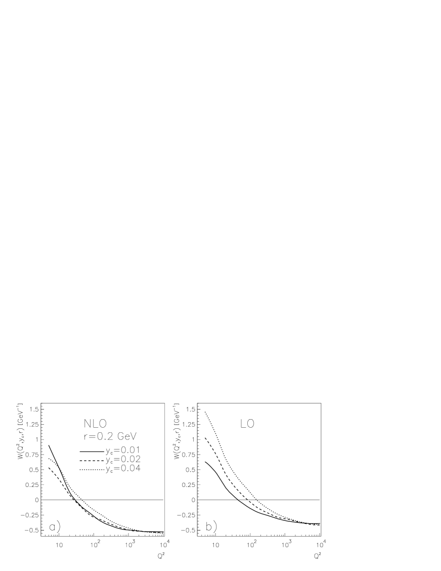
Figure 5: The $Q^{2}$–dependence of $W(Q^{2},y_{c},r=0.2)$ for three different values of $y_{c}$ at the NLO (a) and LO (b). All curves correspond to the case of no cuts.

This value has been extracted from the $Q^{2}$–dependence of $R_{2+1}(Q^{2})$, displayed in Fig. 5 of [4], using only the two highest $Q^{2}$ data points. Within the error bars the value (2) is consistent with the world average, but its accuracy is insufficient to draw any firmer conclusions. Discarding (for reasons discussed in [4]) the three lowest $Q^{2}$ points means not taking into account the region where most of the running of $\alpha_{s}(\mu)$ occurs and where also the data are most sensitive to $\Lambda_{\overline{{\mathrm{MS}}}}\;$. The experimental errors would have to decrease by at least a factor of three to make this way of determining $\alpha_{s}(M_{Z},\overline{{\mathrm{MS}}})$ competitive with the most precise determinations of $\alpha_{s}(M_{Z},\overline{{\mathrm{MS}}})$ based on DIS scattering or LEP event shapes data. Some improvement may be expected already from the ongoing analyses of 1994 data.

There is one aspect of the extraction of $\alpha_{s}$ from the measured ratio (1) crucial for its consistency. In [4] $\alpha_{s}(\mu,\overline{{\mathrm{MS}}})$ (or, equivalently, $\Lambda_{\overline{{\mathrm{MS}}}}$) was considered as a free parameter in the hard scattering cross–sections, but not in the parton distribution functions (PDF), for which the MRSH set was used. The authors of [4] concede that “for strict consistency” one should “reevolve the distributions” using the value of $\alpha_{s}(\mu,\overline{{\mathrm{MS}}})$ obtained in their paper, but claim that given the presently obtainable accuracy “this is not necessary”. However, reevolving PDF, that is solving the evolution equations with the initial conditions corresponding to the MRSH (or any other chosen set of PDF), but using the value of $\Lambda_{\overline{{\mathrm{MS}}}}\;$extracted from (1) instead of the “input” $\Lambda_{\overline{{\mathrm{MS}}}}({\mathrm{MRSH}})$ would solve nothing. Except for the case that the extracted $\Lambda_{\overline{{\mathrm{MS}}}}\;$coincided with the input one, the reevolved PDF would be different from the original MRSH ones. This would require iterating the whole procedure until the extracted value of $\Lambda_{\overline{{\mathrm{MS}}}}\;$coincided with the input one. But then one would have to check whether the resulting new PDF still described the whole body of hard scattering data on which the original global fit was based. Moreover, although mathematically legal exercise, reevolving PDF from unchanged initial conditions with changed $\Lambda_{\overline{{\mathrm{MS}}}}\;$is, as argued in Section 3 below, theoretically inconsistent. In the situation when the measurement of the quantity (1) alone is clearly insufficient to determine $\alpha_{s}$, the only meaningful way of using its results is to include them in the conventional global fits and see what comes out.

Nevertheless, it might be useful to know under which conditions neglecting $\Lambda_{\overline{{\mathrm{MS}}}}\;$in the PDF is numerically good approximation for determining $\alpha_{s}$ from (1). The purpose of our paper is to investigate this question in detail. The paper is organized as follows. In the next section we recall basic relevant formulae and emphasize the importance of considering $\Lambda_{\overline{{\mathrm{MS}}}}\;$in PDF. In Section 3 a simple procedure of constructing PDF for arbitrary $\Lambda_{\overline{{\mathrm{MS}}}}\;$is outlined. Results of numerical simulations in which $\Lambda_{\overline{{\mathrm{MS}}}}\;$is varied separately in hard scattering cross–sections and PDF are presented and discussed in Section 4, followed by conclusions in Section 5. Detailed elaboration of arguments supporting the claim made in Section 2 is left for the Appendix.

2 Basic formulae

We use the couplant $a\equiv\alpha_{s}(\mu)/\pi$ as QCD expansion parameter. It satisfies the equation

$$\frac{{\mathrm{d}}a(\mu,{\mathrm{RS}})}{{\mathrm{d}}\ln\mu}=-ba^{2}(\mu,{\mathrm{RS}})\left(1+ca(\mu,{\mathrm{RS}})+c_{2}a^{2}(\mu,{\mathrm{RS}})+\cdots\right).$$ (3)

For 3 colours and $n_{f}$ massless quark flavours $b=(33-2n_{f})/6,\;c=(153-19n_{f})/(66-4n_{f})$, while all higher order coefficients $c_{k};k\geq 2$ in (3) are free parameters, which define the so called renormalization convention (RC). Together with the specification of the initial condition on the solution of (3) they define the renormalization scheme (RS). To get a unique result of perturbative calculations both the scale $\mu$ and the RS must be specified. Throughout this paper we stay in the conventional $\overline{{\mathrm{MS}}}$ RS and therefore the corresponding specification “$\overline{{\mathrm{MS}}}$” in $\Lambda_{\overline{{\mathrm{MS}}}}\;$as well as in $\alpha_{s}(\mu,\overline{{\mathrm{MS}}})$ will be dropped in the following. The jet cross–sections $\sigma_{k+1}$ in (1) are given as integrals over the parton level cross–sections $C_{k+1,i}$

$$\sigma_{k+1}(Q^{2},y_{c},\Lambda)\equiv\sum_{i}\int^{1}_{0}{\mathrm{d}}xf_{i}(x,M,\Lambda)C_{k+1,i}(Q,M,x,y_{c},\Lambda),$$ (4)

where $f_{i}(x,M)$ are PDF of the proton evaluated at the factorization scale $M$ and the sum runs over all parton species, i.e. quark, antiquarks and gluon. In (4) we have written out explicitly the dependence of both jet and parton level hard scattering cross–sections $\sigma_{k+1},C_{k+1,i}$ as well as of the PDF $f_{i}$ on $\Lambda\;$. This dependence reflects the fact that physical quantities do depend on the value of $\Lambda\;$(in a chosen RS). Contrary to that, jet cross-sections $\sigma_{k+1}$ evaluated to all orders of perturbation theory are independent of both the factorization scale $M$ and the RS. In perturbative QCD the parton level hard scattering cross-sections are given as expansions in the couplant $a(\mu/\Lambda)$, taken at the hard scattering scattering scale $\mu$

$$C_{2+1,i}(Q,M,x,y_{c},\Lambda) = a(\mu/\Lambda)\left[c^{(1)}_{2+1,i}(x,y_{c})+a(\mu/\Lambda)c^{(2)}_{2+1,i}(Q/M,x,y_{c})\right],$$ (5)

$$C_{1+1,i}(Q,M,x,y_{c},\Lambda) = c^{(0)}_{1+1,i}(Q,x)+a(\mu/\Lambda)c^{(1)}_{1+1,i}(Q/M,x,y_{c}).$$ (6)

In standard global analyses of hard scattering processes [14, 15, 16], $\Lambda\;$is fitted together with a set of parameters $a_{i}^{(j)}$, describing distribution functions $p^{(j)}(x,M)$ of parton species $j$ at some initial scale $M_{0}$, usually in the form

$$p^{(j)}(x,M_{0})=a_{0}^{(j)}x^{a_{1}^{(j)}}(1-x)^{a_{2}^{(j)}}\left(1+a_{3}^{(j)}\sqrt{x}+a_{4}^{(j)}x+a_{5}^{(j)}x^{3/2}\right).$$ (7)

To determine the relative importance of varying $\Lambda\;$in PDF and hard scattering cross–sections, we write the derivative ${\mathrm{d}}\sigma_{2+1}/{\mathrm{d}}\ln\Lambda$:

$$\frac{{\mathrm{d}}\sigma_{2+1}(Q^{2},\Lambda)}{{\mathrm{d}}\ln\Lambda}=\sum_{i}\int^{1}_{0}{\mathrm{d}}x\left[\frac{{\mathrm{d}}f_{i}(x,M,\Lambda)}{{\mathrm{d}}\ln\Lambda}a(M)c_{2+1,i}^{(1)}(x)+f_{i}(x,M,\Lambda)c_{2+1,i}^{(1)}(x)\frac{{\mathrm{d}}a(M)}{{\mathrm{d}}\ln\Lambda}\right]=$$ (8)

$$a(M)\sum_{ij}\int^{1}_{0}{\mathrm{d}}x\left[-\int^{1}_{0}\frac{{\mathrm{d}}y}{y}f_{j}(y,M,\Lambda)P^{(0)}_{ij}(z)a(M)c_{2+1,i}^{(1)}(x)+bf_{i}(x,M,\Lambda)a(M)c_{2+1,i}^{(1)}(x)\right],$$

where $z\equiv x/y$ and $P^{(0)}_{ij}(z)$ are the LO AP branching functions . In the above expression we have used (3) and standard evolution equations for PDF, exploited the equality ${\mathrm{d}}a(M/\Lambda)/{\mathrm{d}}\ln M=-{\mathrm{d}}a(M/\Lambda)/{\mathrm{d}}\ln\Lambda$ and took into account that the same relation between derivatives with respect to $M$ and $\Lambda$ holds also for PDF. The first term in the brackets of (8) results from variation of $\Lambda\;$in PDF while the second from variation of $\Lambda\;$in parton level hard scattering cross–sections. Eq. (8) implies that the leading order term of ${\mathrm{d}}\sigma_{2+1}/{\mathrm{d}}\ln\Lambda$ involves merely the LO evolution equations for PDF and leading order term of parton level hard scattering cross–sections $C_{2+1,i}$. The dependence of $\sigma_{2+1}$ on $\Lambda\;$starts therefore already at the LO and consequently also the relative importance of the two terms in the brackets of (8) is basically the LO effect. Note, however, that associating $\Lambda\;$in $\sigma_{2+1}$ with any well-defined RS requires including the NLO corrections as well. Eq. (8) tells us that the variation of $\Lambda\;$in the couplant $a(\mu/\Lambda)$ changes the jet cross–section $\sigma_{2+1}$ by the term of the same order (schematically $O(a)\sigma_{2+1}$) as when $\Lambda\;$is varied in PDF. Consequently if we want to determine $\Lambda\;$from jet cross–section $\sigma_{2+1}$, we must vary it in PDF as well.

For the quantity $R_{2+1}(Q^{2})$ the situation is less obvious. PDF appear in both the numerator and denominator of (1) and so some cancellations might occur, while the hard scattering cross–sections start as $O(a)$ for $C_{2+1,i}$ and as $O(1)$ for $C_{1+1,i}$. Nevertheless as shown in the Appendix also for the ratio $R_{2+1}$ varying $\Lambda\;$in PDF generates terms which are of the same order as those resulting from the variation of $\Lambda\;$in the hard scattering cross-sections $C_{k+1,i}$.

3 Parton distribution functions for arbitrary $\Lambda\;$

In the previous Section we have shown that for a theoretically consistent extraction of $\Lambda\;$from $R_{2+1}(Q^{2})$, $\Lambda\;$must be varied not only in hard scattering cross–sections, but also in the PDF. We now want to investigate the numerical importance of varying $\Lambda\;$in PDF. For this we first have to know what to do with the parameters $M_{0},a^{(j)}_{i}$, specifying the initial conditions (7), when $\Lambda\;$is varied. The obvious choice seems to be to keep them fixed and simply solve the evolution equations with variable $\Lambda\;$. This, however, would be inconsistent with the idea of factorization, which implies that also the initial conditions depend on $\Lambda$!

To see the caveat, let us first consider (3) as well as the evolution equation for the nonsinglet quark distribution function $q_{{\mathrm{NS}}}(x,M)$ at the LO. In term of moments, defined as

$$f(n)\equiv\int^{1}_{0}{\mathrm{d}}xx^{n}f(x)$$ (9)

we have

$$\frac{{\mathrm{d}}q_{{\mathrm{NS}}}(n,M,\Lambda)}{{\mathrm{d}}\ln M}=a(M/\Lambda)q_{{\mathrm{NS}}}(n,M)P^{(0)}_{{\mathrm{NS}}}(n),\;\;d_{n}\equiv-P^{(0)}_{{\mathrm{NS}}}(n)/b,$$ (10)

wherefrom

$$q_{{\mathrm{NS}}}(n,M,\Lambda)=A_{n}\left[a(M/\Lambda)\right]^{d_{n}},\;\;\;a(M/\Lambda)=\frac{1}{b\ln(M/\Lambda)}.$$ (11)

In the above expressions $P^{(0)}_{{\mathrm{NS}}}(n,M)$ are moments of LO nonsinglet AP branching function and $A_{n}$ are dimensionless constants describing the nonperturbative, long distance, properties of the nucleon. These constants are unique pure numbers. Via (11) they determine the asymptotic behavior of $q_{{\mathrm{NS}}}(n,M,\Lambda)$ for $M\rightarrow\infty$ [17] and thus provide alternative way of specifying the initial conditions on the solutions of (10). The separation in (11) of $q_{{\mathrm{NS}}}(n,M,\Lambda)$ into two parts – one calculable in perturbation theory and the other incorporating all the nonperturbative effects – is the essence of the factorization idea [17]. Note that in (11) the dependence on $\Lambda\;$is simply a reflection of its dependence on $M$. Knowing the latter, we know the former. For finite initial $M_{0}$ (11) implies

$$q_{{\mathrm{NS}}}(n,M,\Lambda)=q_{{\mathrm{NS}}}(n,M_{0},\Lambda)\left[\frac{a(M/\Lambda)}{a(M_{0}/\Lambda)}\right]^{d_{n}}=q_{{\mathrm{NS}}}(n,M_{0},\Lambda)\exp(-d_{n}s),$$ (12)

where

$$s\equiv\ln\left(\frac{\ln(M/\Lambda)}{\ln(M_{0}/\Lambda)}\right)\doteq\ln\left(\frac{a(M_{0}/\Lambda)}{a(M/\Lambda)}\right)$$ (13)

is the so called “evolution distance” [16]. The second equality in (13) holds exactly at the leading order and approximately at higher ones. Rewriting (12) again in the form (11)

$$q_{{\mathrm{NS}}}(n,M,\Lambda)=\left[\frac{q_{{\mathrm{NS}}}(n,M_{0},\Lambda)}{\left(a(M_{0}/\Lambda)\right)^{d_{n}}}\right]\left(a(M/\Lambda)\right)^{d_{n}}$$ (14)

we see that the ratio of $q_{{\mathrm{NS}}}(n,M_{0},\Lambda)$ and $(a(M_{0}/\Lambda))^{d_{n}}$ equals the invariant $A_{n}$ and thus is both $M_{0}$ and $\Lambda\;$independent. This, however, is possible only if the initial moments $q_{{\mathrm{NS}}}(n,M_{0},\Lambda)$ do, as already indicated, depend on $\Lambda\;$as well! What happens in (14) is that the $\Lambda\;$and $M_{0}$ dependencies coming from $a(M_{0}/\Lambda)$ in the brackets of (12) cancel those of the initial $q_{{\mathrm{NS}}}(n,\Lambda,M_{0})$. Note that considering $q_{{\mathrm{NS}}}(n,M,\Lambda)$ as a function of $s$, formula (14) implies that entire dependence of $q_{{\mathrm{NS}}}(n,M,\Lambda)$ on $\Lambda\;$comes solely from the term $\ln(M/\Lambda)=1/a(M/\Lambda)$ in (13)! The same happens in the realistic case of coupled quark and gluon evolution equations [18]. The dependence of PDF on $M$ and $\Lambda$ through the evolution distance variable $s$ is then a direct consequence of the above relations for the moments.

To investigate the dependence of PDF on $\Lambda\;$we therefore cannot fix initial conditions at some finite $M_{0}$, specified by $p^{(j)}(x,M_{0})$ in (7), and vary $\Lambda\;$in the evolution equations alone. The preceding discussion also suggests what can be held fixed in the process of varying $\Lambda\;$– the constants $A_{n}$! There is no principal obstacle to carrying out QCD analyses with the initial conditions specified by means of the invariants $A_{n}$, which together with $\Lambda\;$should then be fitted to data. There is also a well developed technique of orthogonal polynomials expansions [19], which could be used for this purpose. There are, however, technical problems in practical implementation of this method. One of them concerns the number of parameters $A_{n}$ required for a specification of initial conditions. As shown in [20], one needs at least 9 to 10 first moments of PDF to achieve sufficient precision in reconstruction of PDF from their moments. That is about twice the number of free parameters used in conventional initial conditions (7) at finite $M_{0}$ and seems too much for any reasonable QCD fit.

However, the preceding paragraph also suggests a simple procedure, which makes use of some of the available parameterizations and generalizes them to arbitrary $\Lambda\;$, keeping, as discussed above, the constants $A_{n}$ fixed. From all the available parameterizations of PDF those given by analytic expressions of the coefficients $a^{(j)}_{i}$ on a general factorization scale $M$ via the variable $s$, defined in (13), are particularly suitable for this purpose. In our studies we took several of the GRV parameterizations, both LO and NLO ones, defined in [21]. At the LO the recipe for construction of PDF for arbitrary $\Lambda\;$is simple:

• Use any of the parameterizations expressing the solutions of evolution equations as functions of the “evolution distance” variable s, defined in (13).

• Keep $\Lambda$ in $\ln(M_{0}/\Lambda)$ fixed at the value obtained in the fit.

• Vary $\Lambda$ in $\ln(M/\Lambda)$.

• Use the original parameterization with variable $s=s(\Lambda)$.

This construction is exact at the LO. At the NLO the couplant $a(M/\Lambda)$ is no longer given simply as $1/\ln(M/\Lambda)$ and consequently the second equality in (13) holds only approximately. This, together with the additional term appearing in the NLO expression for $q_{{\mathrm{NS}}}(n,M,\Lambda)$

$$q_{{\mathrm{NS}}}(n,M,\Lambda,A_{n})=A_{n}\left[\frac{a(M/\Lambda)}{1+ca(M/\Lambda)}\right]^{d_{n}}\left(1+ca(M/\Lambda)\right)^{P^{(1)}_{{\mathrm{NS}}}(n)/bc},$$ (15)

destroy simple dependence of $q_{{\mathrm{NS}}}$ on $M,M_{0}$ and $\Lambda$ via the variable $s$. Using the above recipe for the NLO GRV parameterizations provides therefore merely an approximate solution of our task, but one that is sufficient for the purposes of determining the relative importance of varying $\Lambda\;$in PDF and hard scattering cross–sections.

As an illustration of our procedure we plot in Fig. 1, for $x\geq 10^{-4}$ and two values of $Q^{2}$, the dependence of valence and sea $u$–quark and gluon distribution functions on $\Lambda$. The curves correspond to the LO GRV parameterization of [21]. We see that this dependence decreases with increasing $Q^{2}$, is most pronounced for the gluon distribution function and almost irrelevant for the valence quark one. These features are qualitatively the same as those obtained in refs. [22, 23], which contain results of global fits performed for several fixed values of $\Lambda$. Nevertheless, quantitatively the sensitivity to the variation of $\Lambda\;$, observed in these papers, is markedly weaker than that of our results, displayed in Fig. 1. The reason for this difference is simple. In global analyses of [22, 23] fitting the data for different values of $\Lambda$ leads to different values of boundary condition parameters $a^{(j)}_{i}$, which partially compensates the variation of $\Lambda$. Eqs. (11) or (15) tell us that for any fixed scale $M$ and for any moment $n$ (and thus for any $x$) the change of $\Lambda$ can be fully compensated by an appropriate change of the constants $A_{n}$. For a finite interval of $M$ this compensation cannot be complete, but it is clear that the dependence of the fitted PDF on $\Lambda$ comes out weaker than in our procedure where only $\Lambda$ is varied and all the coefficients $A_{n}$ (or, analogously, $a^{(j)}_{i}$) are held fixed.

4 Numerical results

All the results reported below were obtained using the PROJET 4.1 generator [6]. To quantify the dependence of $R_{2+1}$ on $\Lambda\;$separately in hard scattering cross–sections and PDF we consider it as a function of $Q^{2},y_{c}$ and two independent $\Lambda$–parameters, denoted as $\Lambda^{{\mathrm{hsc}}}$ and $\Lambda^{{\mathrm{pdf}}}$ respectively. The results are then studied subsequently as a function of $\Lambda^{{\mathrm{hsc}}}\;,\Lambda^{{\mathrm{pdf}}}\;,Q^{2}$ and $y_{c}$. First we analyse the case with no cuts on the final state jets and then discuss the changes caused by the imposition of cuts as specified in [4].

4.1 The case of no cuts

The simulations were done at both the leading and next–to–leading order and for

• 12 values of $Q^{2}$ (equidistant in $\ln Q^{2}$) between 5 and $10^{4}$ GeV²,

• 5 values of $\Lambda^{{\mathrm{pdf}}}\;$ or $\Lambda^{{\mathrm{hsc}}}\;$, equal to $0.1,0.2,0.3,0.4$ and $0.5$ GeV,

• 3 values of $y_{c}=0.01,0.02,0.04$.

First we discuss the results of the NLO analysis. Fig. 2 shows a series of plots corresponding to $y_{c}=0.01$ and displaying the dependence of $R_{2+1}$ on $\Lambda^{{\mathrm{hsc}}}\;$ for fixed $\Lambda^{{\mathrm{pdf}}}\;$ (dotted curves) or on $\Lambda^{{\mathrm{pdf}}}\;$ for fixed $\Lambda^{{\mathrm{hsc}}}\;$ (solid curves). Each plot corresponds to one of the 6 selected values of $Q^{2}$. We see that for $Q^{2}$ below about $40$ GeV² the solid curves are steeper that the dotted ones, while above $40$ GeV² the situation is reversed. This means that below $40$ GeV² varying $\Lambda\;$in PDF is more important than varying it in the hard scattering cross–sections for $Q^{2}$, while the opposite holds above $40$ GeV². The same information as in Fig. 2 is displayed in a different manner in Fig. 3, where the $Q^{2}$ dependence of $R_{2+1}$ is plotted for various combinations of $\Lambda^{{\mathrm{pdf}}}\;$ and $\Lambda^{{\mathrm{hsc}}}\;$. The shape of the curves in Fig. 3 is a result of two opposite effects: as $Q^{2}$ increases the phase space available for produced jets increases as well, but at the same time the value of the running $\alpha_{s}(Q/\Lambda)$ decreases. At low $Q^{2}$, on the other hand, phase space shrinks, but $\alpha_{s}(Q/\Lambda)$ grows. The same features of the relative importance of varying $\Lambda^{{\mathrm{pdf}}}\;$ and $\Lambda^{{\mathrm{hsc}}}\;$ as mentioned above are reflected in a bigger spread of the five curves in Figs. 3d)-f) compared to those in Fig. 3a)-c) for $Q^{2}\leq 40$ GeV² and smaller spread above $40$ GeV². Note also that for fixed $\Lambda^{{\mathrm{pdf}}}\;$ the sensitivity to the variation of $\Lambda^{{\mathrm{hsc}}}\;$ is about the same at all $Q^{2}$. The shape of curves in Fig. 2 suggests that the ratio

$$V(Q^{2},y_{c},r,s)\equiv\frac{R_{2+1}(Q^{2},y_{c},\Lambda^{{\mathrm{pdf}}}\;=s,\Lambda^{{\mathrm{hsc}}}\;=r)}{R_{2+1}(Q^{2},y_{c},\Lambda^{{\mathrm{pdf}}}\;=r,\Lambda^{{\mathrm{hsc}}}\;=s)},$$ (16)

is to a good approximation a linear function of $s$ for any fixed $Q^{2},y_{c},r$. Considered as a function of $s$ for fixed $r$, (16) quantifies the relative importance of varying $\Lambda\;$in the PDF (described by $R_{2+1}$ in the numerator) and in hard scattering cross–sections (described by $R_{2+1}$ in the denominator). To summarize the results of Fig. 2 we fitted $V(Q^{2},y_{c},r,s)$ by a linear function of $s$ and defined

$$W(Q^{2},y_{c},r)\equiv\frac{{\mathrm{d}}V^{fit}(Q^{2},y_{c},r,s)}{{\mathrm{d}}s},$$ (17)

which, by construction, is $s$–independent function of $Q^{2},y_{c}$ and $r$. Positive $W$ means that the variation of $\Lambda\;$in the PDF is more important than that in the hard scattering cross–sections, while for negative $W$ the situation is opposite. The $Q^{2}$–dependence of $W(Q^{2},y_{c},r)$ is plotted in Fig. 4a-c for three values of $y_{c}=0.01,0.02,0.04$ and five values of $r=0.1,0.2,0.3,0.4,0.5$ GeV. In Fig. 5a we compare the $Q^{2}$ dependence of $W(Q^{2},y_{c},r=0.2\;{\mathrm{GeV}})$ for different values of $y_{c}=0.01,0.02,0.04$. Similar plots can be drawn for other values of $r$ as well. From Figs. 2–5a we conclude that at the NLO:

• For $Q^{2}$ below about $40$ GeV² the variation of $\Lambda$ is more important in PDF than in the hard scattering cross-sections, while above $40$ GeV² the situation is reversed.

• Above $Q^{2}\approx 10^{3}$ GeV² the variation of $\Lambda\;$in PDF becomes negligible.

• The preceding conclusions depend only weakly on $y_{c}$.

At the LO the general features are the same as those displayed in Figs. 2–5a and we therefore merely summarize them in Fig. 5b. Comparing Figs. 5a and 5b we see that at the LO

• the “cross–over” point $Q^{2}_{cr}$, where $W(Q^{2}_{cr},y_{c},r)=0$, is at higher values of $Q^{2}_{cr}\sim 50-200$ GeV² and depends more sensitively on $y_{c}$, than at the NLO,

• the relative importance of varying $\Lambda\;$in PDF is for almost all values of $Q^{2}$ and $y_{c}$ larger than at the NLO,

• the difference between the LO and NLO results increases with increasing $y_{c}$.

4.2 The case of H1 cuts

In [4] two subsamples of events with jets are defined:

a) high $Q^{2}$ sample: $Q^{2}\geq 100$ GeV²,

b) low $Q^{2}$ sample: $10\leq Q^{2}\leq 100$ GeV².

In both subsamples outgoing jets angle in the HERA lab system was restricted to lie in the interval $10^{\circ}\leq\theta^{{\mathrm{jet}}}_{{\mathrm{lab}}}\leq 145^{\circ}$, but there are also cuts on other variables, in which the two samples differ. In Fig. 6 plots analogous to those of Fig. 3, but incorporating the H1 cuts, are displayed. We see that the experimental cuts suppress the sensitivity of $R_{2+1}(Q^{2})$ to the variation of $\Lambda\;$in the PDF in the low $Q^{2}$ region, while leaving it essentially unchanged the high $Q^{2}$ one. We conclude that in the region $Q^{2}\geq 100$ GeV², used in [4] for the extraction of $\Lambda\;$from the measured $R_{2+1}(Q^{2})$, the variation of $\Lambda\;$in the PDF can be safely neglected.

5 Conclusions

In this paper we have shown that theoretically consistent determination of $\alpha_{s}$ from $R_{2+1}$ in DIS requires the variation of $\Lambda$ in both the hard scattering cross–sections and parton distribution functions. After defining a procedure for the construction of PDF which satisfy the corresponding evolution equations for an arbitrary value of $\Lambda$, we used them to investigate the numerical importance of varying $\Lambda$ in PDF for the quantity $R_{2+1}$. The results of this investigation show that if no cuts are applied on produced jets the variation of $\Lambda$ in PDF

• is more important at the LO than at the NLO,

• is more important than that in the hard scattering cross–sections in low $Q^{2}$ region ($Q^{2}\leq 40$ GeV² at the NLO and $Q^{2}\leq 50-200$ GeV² at the LO),

• can be safely neglected above $Q^{2}\approx 1000$ GeV².

We have also demonstrated that in the low $Q^{2}$ region the sensitivity of $R_{2+1}(Q^{2})$ to the variation of $\Lambda\;$in PDF is strongly suppressed by imposing experimental cuts applied in the H1 paper [4].

Acknowledgement

This work had been supported in part by the grant No. A110136 of the Grant Agency of the Academy of Sciences of the Czech Republic.

Appendix

To show that $\Lambda\;$in PDF must be varied also in the ratio (1) we shall draw on analogy between the cross–sections $\sigma_{k+1}$ and the longitudinal and transverse structure functions $F_{L}$, $F_{2}$ given as

$$\frac{F_{2}(x,Q^{2},\Lambda)}{x}=\int_{x}^{1}\frac{{\mathrm{d}}y}{y}\left[\sum_{i=1}^{12}e_{i}^{2}q_{i}(y,M,\Lambda)C_{q}^{(2)}(z,Q,M,\Lambda)+\sum_{i=1}^{12}e^{2}_{i}G(y,M,\Lambda)C_{G}^{(2)}(z,Q,M,\Lambda)\right],$$ (18)

$$\frac{F_{L}(x,Q^{2},\Lambda)}{x}=\int_{x}^{1}\frac{{\mathrm{d}}y}{y}\left[\sum_{i=1}^{12}e^{2}_{i}q_{i}(y,M,\Lambda)C_{q}^{(L)}(z,Q,M,\Lambda)+\sum_{i=1}^{12}e^{2}_{i}G(y,M,\Lambda)C_{G}^{(L)}(z,Q,M,\Lambda)\right],$$ (19)

where $z=x/y$, the sums run over all quark and antiquark flavours and

$$C_{q}^{(2)}(z,Q,M,\Lambda) = \delta(1-z)+a(M/\Lambda)c^{(2)}_{q}(z,Q/M)+O(a^{2}(M/\Lambda)),$$ (20)

$$C_{G}^{(2)}(z,Q,M,\Lambda) = a(M/\Lambda)c^{(2)}_{G}(z,Q/M)+O(a^{2}(M/\Lambda)),$$ (21)

$$C_{q}^{(L)}(z,Q,M,\Lambda) = a(M/\Lambda)c^{(L)}_{q}(z)+O(a^{2}(M/\Lambda)),$$ (22)

$$C_{G}^{(L)}(z,Q,M,\Lambda) = a(M/\Lambda)c^{(L)}_{G}(z)+O(a^{2}(M/\Lambda)).$$ (23)

The quantity analogous to $R_{2+1}$ is the ratio

$$R_{L}(x,Q^{2},\Lambda)\equiv\frac{F_{L}(x,Q^{2},\Lambda)}{F_{2}(x,Q^{2},\Lambda)+F_{L}(x,Q^{2},\Lambda)}.$$ (24)

In terms of moments (18)-(19) read

$$F_{2}(n-1,Q^{2},\Lambda)=\sum_{i}^{12}e_{i}^{2}q_{i}(n,M,\Lambda)C_{q}^{(2)}(n,Q,M,\Lambda)+\sum_{i=1}^{12}e^{2}_{i}G(n,M,\Lambda)C_{G}^{(2)}(n,Q,M,\Lambda),$$ (25)

$$F_{L}(n-1,Q^{2},\Lambda)=\sum_{i=1}^{12}e^{2}_{i}q_{i}(n,M,\Lambda)C_{q}^{(L)}(n,Q,M,\Lambda)+\sum_{i=1}^{12}e^{2}_{i}G(n,M,\Lambda)C_{G}^{(L)}(n,Q,M,\Lambda).$$ (26)

For moments the quantity analogous to $R_{2+1}(Q^{2})$ is the ratio

$$\overline{R}_{L}(n,Q^{2},\Lambda)\equiv\frac{F_{L}(n-1,Q^{2},\Lambda)}{F_{2}(n-1,Q^{2},\Lambda)+F_{L}(n-1,Q^{2},\Lambda)}.$$ (27)

Note that $\overline{R}_{L}(n,Q^{2},\Lambda)$ defined in (27) is not the moment of the ratio $R_{L}(x)$, but rather the ratio of the moments! We mention the analogy of $R_{2+1}$ to $R_{L}(x)$ and $\overline{R}_{L}(n)$ because all three quantities have similar structure, but the later two are simpler and, moreover, $\overline{R}_{L}(n)$ can be treated analytically. The technique of moments has recently been applied in [24] to a related problem of extracting gluon distribution function from jet production in DIS.

In the expressions for $\sigma_{k+1},R_{2+1}$, as well as for $F_{2,L},R_{L}(x)$ and $\overline{R}_{L}$, we have written out explicitly their dependence on the value of $\Lambda$. Contrary to that, these observables are formally (i.e. order by order of perturbation theory) independent of the factorization scale $M$, the $M$–dependence of PDF being cancelled by that of the hard scattering cross–sections. In the case of $\overline{R}_{L}(n,Q^{2},\Lambda)$, defined in (27), the LO expression reads

$$R_{L}(n,Q^{2},\Lambda) \!\!=\!\! a(M/\Lambda)\frac{\sum_{i}e_{i}^{2}q_{i}(n,M)c_{q}^{(L)}(n)+\left(\sum_{i}e^{2}_{i}\right)G(n,M,\Lambda)c_{G}^{(L)}(n)}{\sum_{i}e^{2}_{i}q_{i}(n,M)}$$ (28)

$$\!\!=\!\! a(M/\Lambda)\left[c_{q}^{(L)}(n)+\frac{\left(\sum_{i}e^{2}_{i}\right)G(n,M,\Lambda)c_{G}^{(L)}(n)}{\sum_{i}e^{2}_{i}q_{i}(n,M,\Lambda)}\right]+\cdots.$$

We see that in the quark contribution to the LO term in (27) quark distribution functions in the numerator and denominator of (27) cancel out

$$\overline{R}_{L}^{{\mathrm{quarks}}}=a(M/\Lambda)c_{q}^{(L)}+\cdots$$ (29)

and $\overline{R}_{L}^{{\mathrm{quarks}}}$ is thus equal to the parton level hard scattering cross–section. This, however, is not the case for the second term in (28), corresponding to gluon contribution, which behaves rather like $a^{1+\Delta(n)}$, where $\Delta(n)$ is, roughly speaking, the difference between gluon and quark LO anomalous dimensions . The cancellation of quark distribution functions in the LO coefficient of (27) is a consequence of the fact that convolutions appearing in (18) and (19) translate to simple multiplications for the respective moments. The above mentioned cancellation holds only for the ratio (27) of moments but not for the ratio (24) of structure functions themselves. This is obvious when we write $F_{2,L}(x,Q^{2})$ as expansions in orthogonal polynomials, which contain infinite sums over different moments of PDF [19, 20]. As a result, even in the quark contribution to $R_{2+1}$ variation of $\Lambda\;$in PDF is in principle equally important as that in hard scattering cross–sections. This conclusion holds for the ratio $R_{2+1}(Q^{2},\Lambda)$ as well.

Figure 1: The dependence of $xu_{v}(x,Q^{2}),xu_{{\mathrm{sea}}}(x,Q^{2})$ and $xG(x,Q^{2})$ of the value $\Lambda^{{\mathrm{pdf}}}\;$ according to the recipe described in the text and for two values of $Q^{2}$. At low $x$, the curves correspond from above to the values of $\Lambda^{{\mathrm{pdf}}}\;$, subsequently, $0.1,0.2,0.3,0.4$ and $0.5$.

Figure 2: The ratio $R_{2+1}(Q,y_{c},\Lambda^{{\mathrm{pdf}}}\;,\Lambda^{{\mathrm{hsc}}}\;)$ as a function of $\Lambda^{{\mathrm{pdf}}}\;$ for fixed $\Lambda^{{\mathrm{hsc}}}\;$ and a series of $Q^{2}$ values (solid lines), or as a function of $\Lambda^{{\mathrm{hsc}}}\;$ for fixed $\Lambda^{{\mathrm{pdf}}}\;$ and the same set of $Q^{2}$ values (dotted lines). The dashed lines correspond to simultaneous variation of $\Lambda^{{\mathrm{pdf}}}\;=\Lambda^{{\mathrm{hsc}}}\;$. Solid curves correspond, from below, to fixed $\Lambda^{{\mathrm{hsc}}}\;=0.1,0.2,0.3,0.4,0.5$ and the dotted to the same fixed values of $\Lambda^{{\mathrm{pdf}}}\;$. In all plots $y_{c}$ equals $0.01$.

Figure 3: (a–c) $Q^{2}$–dependence of the ratio $R_{2+1}(Q,y_{c},\Lambda^{{\mathrm{pdf}}}\;,\Lambda^{{\mathrm{hsc}}}\;)$ for fixed $\Lambda^{{\mathrm{pdf}}}\;=0.1,0.3,0.5$ GeV and five values of $\Lambda^{{\mathrm{hsc}}}\;=0.1,0.2,0.3,0.4,0,5$ GeV. (d–f) The role of $\Lambda^{{\mathrm{pdf}}}\;$ and $\Lambda^{{\mathrm{hsc}}}\;$ is reversed. No cuts were applied in evaluating $R_{2+1}$ and $y_{c}=0.01$. In all plots the curves are ordered from below according to increasing $\Lambda^{{\mathrm{hsc}}}\;$ (in a–c) or $\Lambda^{{\mathrm{pdf}}}\;$ (in d–f).

Figure 4: (a–c) The quantity $W(Q^{2},y_{c},r)$ as a function of $Q^{2}$ for five values of $r$ (given in GeV) and $y_{c}=0.01,0.02,0.04$. All curves correspond to the case of no cuts.

Figure 6: The same as in Fig. 3 but for the H1 acceptance cuts.

References

- [1] S. Bethke, Talk presented at the QCD ’94, Montpellier, France, July 1994, PITHA 94/30.
- [2] B.R. Webber, in: P. Bussey and I. Knowles, eds., Proceedings XXVII International Conference on High Energy Physics (Techno House, Bristol, 1995) 213.
- [3] M. Shifman, UMN-TH-1323-94, hep-ph/9501230
- [4] H1 Collaboration, T. Ahmed et al., Phys. Lett. B 309 (1995) 415.
- [5] ZEUS Collaboration, M. Derrick et al., DESY 95-182.
- [6] D. Graudenz, PROJET 4.1, CERN-TH.7420/94.
- [7] T. Broadkorb, E. Mirkes, DISJET 1.0, MAD/PH/821.
- [8] D. Graudenz, Phys. Lett. B 256 (1991) 518.
- [9] D. Graudenz, Phys. Rev. D 49 (1994) 3291.
- [10] T. Broadkorb, J. Körner, Z. Phys. C 54 (1992) 519.
- [11] T. Broadkorb, E. Mirkes, Z. Phys. C 66 (1995) 141.
- [12] E.W.N. Glover, A.D. Martin, R.G. Roberts and W.J. Stirling, RAL-TR-06-019, hep-ph/9603327.
- [13] CDF Collaboration, F. Abe et al., FERMILAB-PUB-96/020-E.
- [14] A.D. Martin, R.G. Roberts and W.J. Stirling, Phys. Rev. D 47 (1993) 867.
- [15] CTEQ Collab., J. Botts et al., Phys. Lett. B 304 (1993) 159.
- [16] M. Glück, E. Reya and A. Vogt, Z. Phys. C 67 (1995) 433.
- [17] H.D. Politzer, Nucl. Phys. B 192 (1982) 493.
- [18] A. Buras, Rev. Mod. Phys. 52 (1980) 199.
- [19] I. Barker, C. Langensiepen and G. Shaw, Nucl. Phys. B 186 (1981) 61.
- [20] J. Chýla and J. Rameš, Z. Phys. C 31 (1986) 151.
- [21] M. Glück, E. Reya and A. Vogt, Z. Phys. C 53 (1992) 127.
- [22] A. Vogt, Phys. Lett. B 354 (1995) 145.
- [23] A. Martin, G. Roberts and W. J. Stirling, RAL 95–013, hep-ph/9506423.
- [24] D. Graudenz, M. Hampel, Ch. Berger and A. Vogt, DESY 95-107.