Resumming Phase Space Logarithms
in Inclusive Semileptonic $B$ Decays

Abstract

We study logarithms of the form $\ln(m_{q}/m_{b})$ which arise in the inclusive semileptonic decay of a bottom quark to a quark of mass $m_{q}$. We use the renormalization group to resum the leading radiative corrections to these terms, of the form $m_{q}^{2}\alpha_{s}^{n}\ln^{n}(m_{q}/m_{b})$, $m_{q}^{3}\alpha_{s}^{n+1}\ln^{n}(m_{q}/m_{b})$ and $m_{q}^{4}\alpha_{s}^{n}\ln^{n+1}(m_{q}/m_{b})$. The first two resummations are trivial, while the latter involves a non-trivial mixing of four-fermi operators in the $1/m_{b}$ expansion. We illustrate this technique in a toy model in which the semileptonic decay is mediated by a vector interaction, before treating the more complicated case of left-handed decay.

I Introduction

The inclusive semileptonic decay rate of a hadron containing a single bottom quark may be written as a power series in $\Lambda_{\rm QCD}/m_{b}$. The leading term in this expansion is simply the width for the underlying quark-level process $b\rightarrow q\ell\bar{\nu}+qg\ell\bar{\nu}+\dots$, which may be expanded in powers of $\alpha_{s}(m_{b})$,

$$\Gamma={G^{2}_{F}|V_{qb}|^{2}m_{b}^{5}\over 192\pi^{3}}\left[\Gamma^{(0)}(\hat{m}_{q})+{\alpha_{s}(m_{b})\over\pi}\Gamma^{(1)}(\hat{m}_{q})+\left({\alpha_{s}(m_{b})\over\pi}\right)^{2}\Gamma^{(2)}(\hat{m}_{q})+\dots\right].$$ (1)

The coefficients $\Gamma^{(n)}$ are functions of the scaled final quark mass, $\hat{m}_{q}=m_{q}/m_{b}$. When the process is computed at the parton level, the masses arise in limits of the phase space integration, and hence the masses which appear are the perturbatively defined pole masses, $m_{q}=m_{q}^{\rm pole}$. Taking the leptons to be massless, the tree level term is

$$\Gamma^{(0)}(\hat{m}_{q})=1-8\hat{m}_{q}^{2}-24\hat{m}_{q}^{4}\ln\hat{m}_{q}+8\hat{m}_{q}^{6}-\hat{m}_{q}^{8}\,.$$ (2)

The full expression for $\Gamma^{(1)}(\hat{m}_{q})$ has been computed analytically[1], and is quite lengthy; expanding the result in powers of $\hat{m}_{q}$ gives

$$\Gamma^{(1)}(\hat{m}_{q}) = {25\over 6}-{2\pi^{2}\over 3}-\left({136\over 3}+32\ln\hat{m}_{q}\right)\hat{m}_{q}^{2}+{64\pi^{2}\over 3}\hat{m}_{q}^{3}$$ (6)

$$-\left(182+{32\pi^{2}\over 3}-48\ln\hat{m}_{q}+96\ln^{2}\hat{m}_{q}\right)\hat{m}_{q}^{4}$$

$$\mbox{}+{64\pi^{2}\over 3}\hat{m}_{q}^{5}-\left({2104\over 27}-{608\over 9}\ln\hat{m}_{q}\right)\hat{m}_{q}^{2}$$

$$\mbox{}-\left({8857\over 2700}+{2\pi^{2}\over 3}-{32\over 15}\ln\hat{m}_{q}+{8\over 3}\ln^{2}\hat{m}_{q}\right)\hat{m}_{q}^{8}+{\cal O}(\hat{m}_{q}^{10})\,.$$

At order $\alpha_{s}^{2}$, only the graphs containing gluon vacuum polarization have been calculated, and only numerically. For example [2]

$$\Gamma^{(2)}(0) = (-3.44\beta_{0}+c_{1})\,,$$ (7)

$$\Gamma^{(2)}(0.37) = (-0.75\beta_{0}+c_{2})\,,$$ (8)

where $c_{1}$ and $c_{2}$ denote terms not proportional to $\beta_{0}=11-2n_{f}/3$.

Since inclusive semileptonic bottom decays provide a means of measuring the CKM mixing angle $|V_{cb}|$, it is useful to have as much information as possible about the size of the higher order corrections to $\Gamma$. In this paper, we use the operator product expansion and the renormalization group to sum to all orders leading logarithms of the form $\hat{m}_{q}^{4}\alpha_{s}^{n}\ln^{n+1}\hat{m}_{q}$, for $n\geq 0$, as well as terms of the form $\hat{m}_{q}^{2}\alpha_{s}^{n}\ln^{n}\hat{m}_{q}$ and $\hat{m}_{q}^{3}\alpha_{s}^{n+1}\ln^{n}\hat{m}_{q}$. We will show that these corrections are straightforward to calculate using the renormalization group.

We will see that the resummation of the “phase space” logarithms $\hat{m}_{q}^{4}\alpha_{s}^{n}\ln^{n+1}\hat{m}_{q}$ is particularly interesting, and it is to them that we will pay the most attention in what follows. However, because of the prefactor $\hat{m}_{q}^{4}$, these terms are not dominant as $\hat{m}_{q}\to 0$, or in any other limit of the theory. In fact, they are smaller, in principle, than uncomputed terms of the form $\hat{m}_{q}^{2}\alpha_{s}^{n-1}\log^{n}\hat{m}_{q}$, since $\hat{m}_{q}\log\hat{m}_{q}\to 0$ as $\hat{m}_{q}\to 0$. On the other hand, since $\hat{m}_{c}$ is not particularly small, these terms may be numerically significant for $b\rightarrow c$ decays.

Unfortunately, by the same token $\hat{m}_{c}\sim 0.37$ is such a poor expansion parameter that the terms which we can compute using the renormalization group do not dominate those which we cannot compute as easily, and so these results may not be used directly to estimate the size of the higher order corrections to $b\rightarrow X_{c}\ell\bar{\nu}$ decays. This is clear from examining the sizes of the various terms which contribute to $\Gamma^{(0)}$ and $\Gamma^{(1)}$:

$$\Gamma^{(0)}(0.37) = 1-1.095+0.448+0.021-0.0004+\dots=0.372$$ (9)

$$\Gamma^{(1)}(0.37) = -2.41-1.85+10.67-8.06+1.46-0.372-0.005+\dots=-0.568.$$ (10)

where the order of the terms is the same as in Eqs. (2) and (6), and we have included terms up to ${\cal O}(\hat{m}_{c}^{8})$ in the expression for $\Gamma^{(1)}$. Significant cancelations occur in both expressions between terms of different order in $\hat{m}_{c}$; in particular, there is a large cancelation between the ${\cal O}(\alpha_{s}\hat{m}_{c}^{3})$ and ${\cal O}(\alpha_{s}\hat{m}_{c}^{4})$ terms. Similarly, we will find when expanding our resummed results that there is a large contribution (larger than the tree level rate!) at ${\cal O}\left(\alpha_{s}^{2}\hat{m}_{c}^{3}\ln\hat{m}_{c}\right)$. In analogy with the one-loop expression, we might expect a large cancelation between this term and the order $\alpha_{s}^{2}\hat{m}_{c}^{4}\ln\hat{m}_{c}$ term. However, this latter term is down by two powers of $\ln\hat{m}_{c}$ relative to the terms which we are resumming (requiring a three-loop anomalous dimension to resum), and so we have not calculated it. The motivation for our analysis is the insight it will afford us into the origin of a variety of higher order terms in the expression for the semileptonic width, rather than in any reliable estimate of the true size of higher order corrections.

We will use the operator product expansion (OPE) and the heavy quark effective theory (HQET) [3, 4, 5, 6, 7, 8] in our analysis. The application of OPE techniques to inclusive semileptonic heavy quark decays was suggested in Refs. [9, 10], in which two distinct, but ultimately equivalent, methods were introduced. The two approaches differ in the treatment of the leptons in the final state. Since the leptons interact only weakly and electromagnetically with the quark currents which mediate the hadronic decay, there is freedom to integrate over their momenta at various stages of the calculation.

Let us consider the decay $B(P_{B})\to X_{c}(P_{X})+(\ell\bar{\nu})(q)$. This process is mediated by a term in the weak Hamiltonian,

$${\cal H}_{W}=\dots+{G_{F}V_{cb}\over\sqrt{2}}\,\overline{c}\gamma^{\mu}1-\gamma_{5})b\,\overline{\ell}\gamma_{\mu}(1-\gamma_{5})\nu\,.$$ (11)

In the approach of Ref. [9], the Hamiltonian is explicitly factorized into a product of a quark current, $J^{\mu}_{h}$ and a lepton current $J^{\mu}_{\ell}$. Then the differential rate ${\rm d}\Gamma/{\rm d}q^{2}\,{\rm d}q\cdot v$ is written as

$${{\rm d}\Gamma_{B\to X_{c}\ell\nu}\over{\rm d}q^{2}\,{\rm d}q\cdot v}\sim L_{\mu\nu}(q^{2},q\cdot v)W^{\mu\nu}(q^{2},q\cdot v)\,,$$ (12)

where $v^{\mu}=P_{B}^{\mu}/m_{B}$ is the velocity of the $B$ meson and $L_{\mu\nu}$ is the spin summed lepton tensor ($L_{\mu\nu}\propto(q_{\mu}q_{\nu}-g_{\mu\nu}q^{2})$ for massless leptons.) The nonperturbative hadronic tensor $W^{\mu\nu}$ is related via the optical theorem to the imaginary part of the forward scattering amplitude [9, 10],

$$W^{\mu\nu} = \sum_{X_{c}}\langle B|\,J_{h}^{\mu\dagger}\,|X_{c}\rangle\langle X_{c}|\,J_{h}^{\nu}\,|B\rangle(2\pi)^{4}\delta^{4}(P_{B}-P_{X}-q)$$ (13)

$$= -2\,{\rm Im}\,\langle B|\,i\int{\rm d}x\,e^{-iq\cdot x}\,T\left\{J_{h}^{\mu\dagger}(x),J_{h}^{\nu}(0)\right\}\,|B\rangle\,.$$ (14)

The time-ordered product is then written via an operator product expansion as a power series in $\alpha_{s}(m_{b})$ and $1/m_{b}$, as illustrated in Fig. 1. The resulting expression for the differential rate consists of a series of delta functions and derivatives of delta functions at the threshold for $c$ quark production, followed by a cut in the complex $q\cdot v$ plane corresponding to gluon bremsstrahlung. When integrated over the appropriate variables, this yields a sensible prediction for differential decay widths as well as for the total semileptonic width. In this approach, the factor of $\hat{m}_{c}^{4}\ln\hat{m}_{c}$ in Eq. (2) arises from the integration over the phase space variables $q$ and $q\cdot v$. It is important to note that this term is not related to the running of the operators in the OPE between $\mu=m_{b}$ and $\mu=m_{c}$, since this running is performed before any phase space integrals are performed.

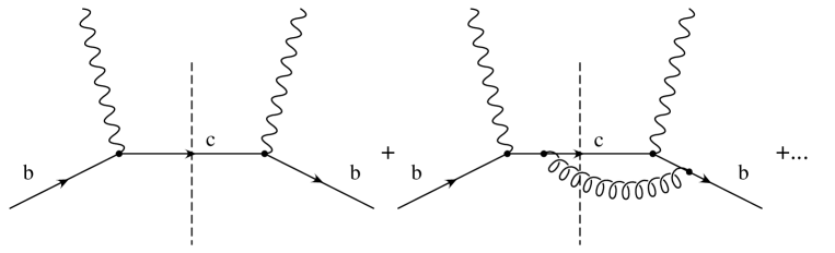
FIG. 1.: Typical diagrams contributing to ${\rm Im}\,T\{J^{\mu\dagger},J^{\nu}\}$.

By contrast, in the approach of Ref. [10] the OPE is performed on the expression for the total, rather than the differential, rate. Once again, the width is written as the imaginary part of the forward scattering amplitude,

$$\Gamma_{B\rightarrow X_{c}\ell\nu} \sim \sum_{X_{c}}{\rm Im}\,{\cal A}(B\rightarrow X_{c}e\bar{\nu}\rightarrow B)$$ (15)

$$\sim {\rm Im}\langle B|T\{{\cal H}_{W}^{\dagger},{\cal H}_{W}\}|B\rangle\,.$$ (16)

This version of the time ordered product is illustrated in Fig. 2. While this approach is completely equivalent to the other, performing the OPE after the integration over the lepton momenta gives us more insight into the origin of the terms involving $\ln\hat{m}_{c}$.

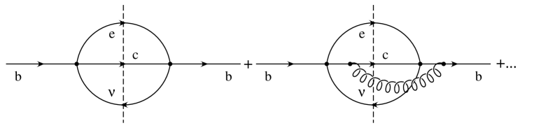
FIG. 2.: Diagrams contributing to ${\rm Im}\,T\{{\cal H}_{W}^{\dagger},{\cal H}_{W}\}$.

When the OPE is performed at the renormalization scale $\mu=m_{b}$, the time ordered product in Eq. (15) is written as a sum of local operators,

$$\left.{\rm Im}\,T\{{\cal H}_{W}^{\dagger},{\cal H}_{W}\}\right|_{\mu=m_{b}} \longrightarrow a_{1}(m_{b})\,\overline{b}\,b+{1\over m_{b}^{2}}\left\{a_{21}(m_{b})\hat{m}_{c}^{2}\,\overline{b}\,b+a_{22}(m_{b})\overline{b}\,({\rm iD})^{2}\,b\right.$$ (18)

$$+\left.a_{23}(m_{b})\overline{b}\,\sigma_{\mu\nu}G^{\mu\nu}\,b\right\}+{\cal O}\left({1/m_{b}^{3}}\right)$$

(note that only the imaginary part of the time ordered product is needed). At the matching scale there are no factors of $\ln\hat{m}_{c}$ in the coefficient functions $a_{ij}(m_{b})$; these logarithms are infrared effects which are contained in the matrix elements of local operators. However, since none of the operators at order $1/m_{b}^{2}$ contains explicit $c$ quarks, none of their matrix elements depend on $m_{c}$ at leading order in $\alpha_{s}$; therefore there is no term proportional to $\hat{m}_{c}^{2}\ln\hat{m}_{c}$ in the tree level expression (2) for the semileptonic decay rate. The first operators of interest which contain explicit $c$ quarks are four quark operators of the form $\overline{b}\Gamma_{1}c\,\overline{c}\Gamma_{2}b$. These arise in the matching due to the graph in Fig. 3 and are of relative order $1/m_{b}^{3}$.

FIG. 3.: Contribution to the coefficient function of $\overline{b}\Gamma_{1}c\,\bar{c}\Gamma_{2}b$ in the OPE of ${\rm Im}\,T\{{\cal H}_{W}^{\dagger},{\cal H}_{W}\}$.

In the next section we will consider a toy model in which the $b$ quark decays via a vector current. In this model, the operator $\bar{h}h\,\bar{c}c$ arises at order $1/m_{b}^{3}$ in the OPE; its matrix element between $b$ quarks is given by the diagram in Fig. 4, giving a contribution of order $\hat{m}_{c}^{3}\ln\hat{m}_{c}$ to the total inclusive rate. For the physically relevant case of a left handed current the corresponding operator is $\bar{h}h\,\bar{c}\hbox to0.0pt{/\hss}vc$, for which the graph in Fig. 4 vanishes. This explains the lack of a term of order $\hat{m}_{c}^{3}\ln\hat{m}_{c}$ in the total inclusive rate (2). In this case, the first logarithm of $\hat{m}_{c}$ arises at order $1/m_{b}^{4}$, in the matrix element of the operator $\hat{m}_{c}\bar{h}h\,\bar{c}c$, giving the term of order $\hat{m}_{c}^{4}\ln\hat{m}_{c}$ in the inclusive decay rate.

Rather than leave these logarithms in the matrix elements of local operators, it is convenient to scale the theory down to the renormalization point $\mu=m_{c}$, at which point the $c$ quark is integrated out of the theory. Below this scale matrix elements can no longer depend on $m_{c}$; all such dependence has been transferred to the coefficient functions in the OPE. By including the leading QCD corrections in the renormalization group equation, the complete series of leading logarithms of the form $\hat{m}_{c}^{n}\alpha_{s}^{n}\ln^{n+1}\hat{m}_{c}$ may be resummed,

$$c_{0}\hat{m}_{c}^{n}\ln\hat{m}_{c}\rightarrow\hat{m}_{c}^{n}\left(c_{0}\ln\hat{m}_{c}+c_{1}\alpha_{s}\ln^{2}\hat{m}_{c}+c_{2}\alpha_{s}^{2}\ln^{3}\hat{m}_{c}+\dots\right)\,,$$ (19)

where $n=3$ for a vector current and $n=4$ for a left handed current. This calculation is technically more complicated for a left-handed current than a vector current, since it involves the renormalization of the complete set of dimension seven operators. Therefore we will warm up in the next section with the simpler case of a vector current, before proceeding on to the realistic decay.

FIG. 4.: Contracting the charm quark fields in a four fermion operator gives a $\ln(m_{c}/m_{b})$ contribution to the semileptonic width.

II Decays via a vector current

We consider the decay mediated by the hadronic current $\overline{c}\gamma^{\mu}b$, coupled to the usual left-handed massless leptons. At tree level, the decay width of the $b$ quark is given by

$$\Gamma_{V} = \Gamma_{V0}\big{[}1-2\hat{m}_{c}-8\hat{m}_{c}^{2}-18\hat{m}_{c}^{3}+18\hat{m}_{c}^{5}+8\hat{m}_{c}^{6}+2\hat{m}_{c}^{7}-\hat{m}_{c}^{8}$$ (21)

$$\mbox{}\qquad\qquad-24\hat{m}_{c}^{3}\log\hat{m}_{c}-24\hat{m}_{c}^{4}\log\hat{m}_{c}-24\hat{m}_{c}^{5}\log\hat{m}_{c}\big{]},$$

where $\Gamma_{V0}=m_{b}^{5}/192\pi^{3}$. The total decay rate may be written via the optical theorem in terms of the imaginary part of the forward scattering amplitude. Integrating explicitly over the leptons, this may be recast as the expectation value of the time-ordered product of the hadronic current and its conjugate,

$$\Gamma_{V}={1\over 2m_{B}}\int{\rm d}q\,e^{-iq\cdot x}\,\langle B|\,T\{\overline{b}\gamma^{\mu}c(x),\overline{c}\gamma^{\nu}b(0)\}\,|B\rangle\times{1\over 3\pi}\left(q_{\mu}q_{\nu}-q^{2}g_{\mu\nu}\right)\,.$$ (22)

The integral is taken over physical values of the total lepton four-momentum $q^{\mu}$.

We now develop the time-ordered product in an operator product expansion. The momentum transfer is of order $m_{b}^{2}$ over almost the entire region of integration, so we organize the expansion in inverse powers of $m_{b}$ rather than in inverse powers of $q^{2}$. Simultaneously, we will expand the ordinary $b$ quark field in terms of the mass-independent HQET field $h$, defined by [8]

$$h(x)={1+\hbox to0.0pt{/\hss}v\over 2}\,\exp(im_{b}v\cdot x)\,b(x)\,.$$ (23)

Here $v^{\mu}=p_{b}^{\mu}/m_{b}$ is the four-velocity of the $b$ quark, which is fixed in the limit $m_{b}\to\infty$ [5]. The Dirac matrix $(1+\hbox to0.0pt{/\hss}v)/2$ projects onto the heavy quark part of the field operator, so $h$ is a two-component, rather than a four-component, object. The exponential factor cancels out the large “on-shell” part of the $b$ quark momentum. This procedure will make all dependence on the heavy quark mass $m_{b}$ explicit in the operator product expansion.

We will order operators in inverse powers of $m_{b}$. The operators of dimension less than six can have no more than two fermion fields, which must be $h$ and $\overline{h}$, since we are interested in the heavy quark decay process. The $c$ quark fields are contracted; the integral over the $c$ quark momentum $p^{\mu}$ is equivalent to the integral over the lepton momentum $q^{\mu}=p_{b}^{\mu}-p^{\mu}$ in Eq. (22). The leading operator, then, is of dimension three:

$${m_{b}^{5}\over 192\pi^{3}}\,\overline{h}\,h=\Gamma_{V0}\,\overline{h}\,h\,.$$ (24)

The matrix element of $\overline{h}\,h$ may be expanded in inverse powers of $m_{b}$ [5],

$$\langle B|\,\overline{h}\,h\,|B\rangle=2m_{B}\big{[}1+{\cal O}(1/m_{b}^{2})\big{]}\,,$$ (25)

where all $1/m_{b}^{n}$ corrections are independent of $\hat{m}_{c}$. Hence the leading operator reproduces the $\hat{m}_{c}=0$ decay rate $\Gamma_{V0}$.

The next operator in the expansion in $1/m_{b}$ is of dimension four,

$$-2\Gamma_{V0}\,\hat{m}_{c}\,\overline{h}\,h\,.$$ (26)

The factor of $\hat{m}_{c}$ is an explicit part of the operator, including its dependence on $\mu$. The operator $\overline{h}\,h$ is a conserved current in the HQET and does not run [11]. Since the operator product expansion is performed at the scale $\mu=m_{b}$, it is $m_{c}(m_{b})$ which appears in the matching. Since $m_{b}$ does not run below $\mu=m_{b}$, neither does the combination $\hat{m}_{c}(m_{b})\overline{h}\,h$. However, leading logarithms are generated if the decay rate is expressed, as it usually is, in terms of $m_{c}(m_{c})$ or $m_{c}^{\rm pole}$. All of these logarithms are resummed if we leave $m_{c}(m_{b})$ unexpanded. The situation is analogous for the dimension five operator

$$-8\Gamma_{V0}\,\hat{m}_{c}^{2}\,\overline{h}\,h\,.$$ (27)

Matching at $\mu=m_{b}$ yields $m_{c}(m_{b})$ in Eqs. (26) and (27), which resums the leading logarithms of the form $\alpha_{s}^{n}\log^{n}\hat{m}_{c}$ in these terms. We note that there are other operators which arise at dimension five and higher, such as $\overline{h}(iD)^{2}h$ and $\overline{h}\sigma_{\mu\nu}G^{\mu\nu}h$, but the matrix elements of these operators are proportional to QCD scale quantities such as $\lambda_{1}$ and $\lambda_{2}$ and do not yield powers of $\hat{m}_{c}^{n}$ [12]. They are included in an analysis which treats the nonperturbative power corrections to the parton model decay [13, 14, 15, 16, 17].

At dimension six we first encounter the four-fermion operators of the form $\overline{h}\Gamma_{1}c\,\overline{c}\Gamma_{2}h$, which give rise at tree level to the term proportional to $\hat{m}_{c}^{3}\log\hat{m}_{c}$ in the total decay rate. We will now compute the leading logarithmic improvement of these terms. Keeping the leading powers of $m_{b}$ in the lepton tensor $(q_{\mu}q_{\nu}-q^{2}g_{\mu\nu})/3\pi$, the operator product expansion yields the dimension six operator

$$\overline{h}\gamma^{\mu}c\,\overline{c}\gamma^{\nu}h\times{m_{b}^{2}\over 3\pi}(v_{\mu}v_{\nu}-g_{\mu\nu})\,.$$ (28)

With the identity $\hbox to0.0pt{/\hss}vh=h$ on the HQET field, this reduces to

$${m_{b}^{2}\over 3\pi}\left[\overline{h}c\,\overline{c}h-\overline{h}\gamma^{\mu}c\,\overline{c}\gamma_{\mu}h\right].$$ (29)

These operators are matched onto at the scale $\mu=m_{b}$. Closing the charm quark loop, they mix with the operator $\hat{m}_{c}^{3}\,\overline{h}\,h$ at order $\alpha_{s}^{0}$, yielding the “phase space” logarithm $-24\Gamma_{V0}\hat{m}_{c}^{3}\log\hat{m}_{c}$. To resum the leading logarithms, we must consider the QCD renormalization of the dimension six operators. However, we do not need the QCD correction to the mixing of the four quark operators with the quark bilinears, which is subleading and will only produce terms in the rate proportional to $\hat{m}_{c}^{3}\alpha_{s}^{n}\log^{n}\hat{m}_{c}$.

The renormalization of the four quark operators simplifies considerably if we first apply a Fierz transformation to bring them into the form $\overline{h}\Gamma_{1}h\,\overline{c}\Gamma_{2}c$. We use the $SU(3)$ identity

$$\delta_{il}\,\delta_{kj}=2\,T^{a}_{ij}\,T^{a}_{kl}+\frac{1}{3}\,\delta_{ij}\,\delta_{kl}\,,$$ (30)

on the color indices, and include a factor of $-1$ from the exchange of the fermion fields $h$ and $c$. The Fierz transformation yields a linear combination of operators of the form

$${\cal O}^{1}_{a}=\overline{h}\Gamma_{a}h\,\overline{c}\Gamma_{a}c\qquad{\rm and}\qquad{\cal O}^{8}_{a}=\overline{h}\Gamma_{a}T^{a}h\,\overline{c}\Gamma_{a}T^{a}c\,,$$ (31)

where $\Gamma_{a}=1,\gamma^{5},\gamma^{\mu},\gamma^{\mu}\gamma^{5},\sigma^{\mu\nu}$. However, because the heavy field $h$ has only two components, there are actually just four independent scalars of the form $\overline{h}\Gamma h$. It is straightforward to show, then, that the allowed Dirac structures for the dimension six operators are

$$\overline{h}\,h\,\overline{c}\,c\,,$$ (32)

$$\overline{h}\,h\,\overline{c}\hbox to0.0pt{/\hss}vc\,,$$ (33)

$$\overline{h}\gamma^{\mu}\gamma^{5}h\,\overline{c}\gamma^{\mu}\gamma^{5}c\,,$$ (34)

$$\overline{h}\gamma^{\mu}\gamma^{5}h\,\overline{c}\hbox to0.0pt{/\hss}v\gamma^{\mu}\gamma^{5}c\,.$$ (35)

With both singlet and octet color structures, we find a set of eight operators.

In the HQET, the coupling of a gluon to a heavy quark line is given by the Feynman rule $v\cdot A$, where $A^{\mu}$ is the gluon field [8]. In $v\cdot A=0$ gauge, in which the gluon does not couple directly to the heavy quark, we see that the renormalization of ${\cal O}^{1}_{a}$ and ${\cal O}^{8}_{a}$ is restricted to the $\overline{c}\Gamma c$ part of the operator. Since for $\hat{m}_{c}=0$ the addition of a gluon loop to $\overline{c}\Gamma c$ generates an even number of Dirac matrices and no $\gamma^{5}$, none of the eight dimension six operators mix with each other under renormalization. Hence the running of these eight operators is multiplicative, except for the color octet $\overline{h}T^{a}h\,\overline{c}\hbox to0.0pt{/\hss}vT^{a}c$, which mixes via “penguin” diagrams with the flavor $SU(3)$ singlet operator $\overline{h}T^{a}h\,\overline{q}_{i}\hbox to0.0pt{/\hss}vT^{a}q_{i}$, with $i$ summed over $u,d,s$.

The dimension six operators mix with quark bilinears at order $\alpha_{s}^{0}$ by contracting the charm quark fields as in Fig. 4. However, only the color singlet, scalar-scalar operator

$${\cal O}_{6}=\overline{h}\,h\,\overline{c}\,c$$ (36)

has a color and Dirac structure such that this mixing, to $\hat{m}_{c}^{3}\overline{h}\,h$, is nonvanishing. Hence it is the only operator which we must consider. The Fierz transformation of the operators (29) yields the coefficient function

$$C_{6}(m_{b})={m_{b}^{2}\over 12\pi}\,.$$ (37)

$C_{6}(\mu)$ runs according to the renormalization group equation

$$\mu{{\rm d}\over{\rm d}\mu}\,C_{6}(\mu)=\gamma_{6}\,C_{6}(\mu)\,,$$ (38)

where a simple HQET calculation yields (via the graphs in Fig. 5)

$$\gamma_{6}=-{g^{2}(\mu)\over 2\pi^{2}}\,.$$ (39)

Solving the differential equation (38) by standard methods, we find

$$C_{6}(\mu)={m_{b}^{2}\over 12\pi}\,\left[{\alpha_{s}(\mu)\over\alpha_{s}(m_{b})}\right]^{12/25}\,.$$ (40)

We now turn to the renormalization of the term $C_{3}(\mu)\hat{m}_{c}^{3}(\mu)\overline{h}\,h$. The coefficient $C_{3}(\mu)$ runs both because of the renormalization of the operator

$${\cal O}_{3}=\hat{m}_{c}^{3}\overline{h}\,h\,,$$ (41)

and because of the mixing from ${\cal O}_{6}$. It obeys the renormalization group equation

$$\mu{{\rm d}\over{\rm d}\mu}\,C_{3}(\mu)=\gamma_{3}\,C_{3}(\mu)+\gamma_{63}\,C_{6}(\mu)\,.$$ (42)

Since the current $\overline{h}\,h$ is conserved, the anomalous dimension $\gamma_{3}$ is given solely by the renormalization of the mass $\hat{m}_{c}(\mu)$,

$$\gamma_{3}=3\gamma_{m}=-{3g^{2}(\mu)\over 2\pi^{2}}\,.$$ (43)

The mixing of ${\cal O}_{6}$ with ${\cal O}_{3}$ is given by contracting the charm quark fields as in Fig. 4,

$$\gamma_{63}={3\over 2\pi^{2}}\,m_{b}^{3}\,.$$ (44)

Because the graph has a cubic divergence, it is proportional to $m_{c}^{3}$; hence $\gamma_{63}$ is proportional to $m_{b}^{3}$.

Solving the differential equation (42) for $C_{3}(\mu)$ and setting $\mu=m_{c}$, we find

$$C_{3}(m_{c})={m_{b}^{5}\over 192\pi^{3}}\,\hat{m}_{c}^{3}{144\pi\over 23\alpha_{s}(m_{c})}\,\left[z^{12/25}-z^{-11/25}\right]\,,$$ (45)

where

$$z={\alpha_{s}(m_{c})\over\alpha_{s}(m_{b})}>1\,.$$ (46)

Note that because the numerator in the expression (45) vanishes as $z\to 1$, the solution for $C_{3}(\mu)$ is well behaved in the limit $\alpha_{s}(m_{c})\to 0$. Expanding $C_{3}(\mu)$ in powers of $\alpha_{s}(m_{c})$, we find

$$C_{3}(m_{c})=\Gamma_{V0}\,\hat{m}_{c}^{3}\left[-24\ln\hat{m}_{c}-48{\alpha_{s}(m_{c})\over\pi}\ln^{2}\hat{m}_{c}+\dots\right]\,.$$ (47)

For $\alpha_{s}(m_{c})=0.41$ and $\hat{m}_{c}=0.37$ (for which $\alpha_{s}(m_{b})=0.27$ and $z=1.54$), we find that the contribution of this operator to the total rate is of order one:

$$C_{3}(m_{c})=\Gamma_{V0}\,[1.22-0.21+\dots]=\Gamma_{V0}\,[0.99]\,.$$ (48)

The resummed logs change the total decay rate by $18\%$. In terms of the quantities $\hat{m}_{c}(m_{b})$ and $\alpha_{s}(m_{b})$ renormalized at the scale $\mu=m_{b}$, we find

$$\Gamma=\Gamma_{V0}\bigg{\{}1 -2\hat{m}_{c}(m_{b})-8\hat{m}_{c}^{2}(m_{b})-18\hat{m}_{c}^{3}(m_{b})\ln\hat{m}_{c}$$ (50)

$$\mbox{}+{144\pi\over 23\alpha_{s}(m_{b})}\hat{m}_{c}^{3}(m_{b})\left(z^{23/25}-1\right)+\dots\bigg{\}}\,.$$

Note that although we include the term $-18\hat{m}_{c}^{3}(m_{b})\ln\hat{m}_{c}$ in this renormalization group improved expression, there are also uncomputed terms of the same order from the two-loop renormalization of the dimension six operators.

III Decays via a left-handed current

We now apply the same analysis to the physical situation of decays mediated by the left-handed current $J^{\mu}=\overline{b}\gamma^{\mu}(1-\gamma^{5})c$. Including the coupling $G_{F}V_{cb}/\sqrt{2}$, the total decay rate is related to the forward scattering amplitude via

$$\Gamma={1\over 2m_{B}}{G_{F}^{2}|V_{cb}|^{2}\over 2}\int{\rm d}q\,e^{-iq\cdot x}\,\langle B|\,T\{J^{\mu\dagger}(x),J^{\nu}(0)\}\,|B\rangle\times{1\over 3\pi}\left(q_{\mu}q_{\nu}-q^{2}g_{\mu\nu}\right)\,.$$ (51)

The tree level rate is $\Gamma_{0}=G_{F}^{2}|V_{cb}|^{2}m_{b}^{5}/192\pi^{3}$. We now expand the time ordered product in an operator product expansion, as before. At tree level, and for dimension $n<6$, we find

$${\Gamma_{0}\over 2m_{B}}\left[\overline{h}\,h-8\hat{m}_{c}^{2}(m_{b})\overline{h}\,h\ +\dots\right]\,,$$ (52)

where the OPE is performed at the renormalization scale $\mu=m_{b}$. The HQET field $h(x)$ is given in Eq. (23), and the lowest order matrix element of $\overline{h}\,h$ in Eq. (25). The ellipses denote charm-independent dimension five operators such as $\overline{h}({\rm iD})^{2}h$, which do not induce terms proportional to $\hat{m}_{c}^{n}$. As before, the combination $\hat{m}_{c}^{2}\overline{h}\,h$ does not run below $\mu=m_{b}$; expanding $\hat{m}_{c}(m_{b})$ in terms of $m_{c}^{\rm pole}$, one finds at leading logarithmic order

$$-8m_{c}^{2}(m_{b})=-8(m_{c}^{\rm pole})^{2}\,z^{-24/25}=(m_{c}^{\rm pole})^{2}\left[-8-32\alpha_{s}(m_{b})\ln\hat{m}_{c}+{8\over 3}\alpha_{s}(m_{b})^{2}\ln^{2}\hat{m}_{c}+\dots\right]\,,$$ (53)

where $z=\alpha_{s}(m_{c})/\alpha_{s}(m_{b})$. Hence we reproduce the order $\alpha_{s}$ correction from $\Gamma^{(1)}$ (6), and then extend this result to resum all logarithms of the form $\hat{m}_{c}^{2}\alpha_{s}^{n}\ln^{n}\hat{m}_{c}$ in the coefficient functions $\Gamma^{(n)}$. (This constraint on the $m_{c}^{2}\alpha_{s}\log\hat{m}_{c}$ was also noted by Nir [1]).

At dimension six, four quark operators of the form $\overline{h}\Gamma_{1}h\,\overline{c}\Gamma_{2}c$ arise, just as in the case of vector decays. In principle, these operators could induce terms of order $\hat{m}_{c}^{3}\ln\hat{m}_{c}$ in the total decay rate, when they mix with $\overline{h}\,h$. Expanding the operator product, applying the Fierz transformation, and dropping parity-odd operators which cannot contribute to the forward matrix element, we find the dimension six operators

$${\Gamma_{0}\over 2m_{B}}{32\pi^{2}\over m_{b}^{3}}\left[-{1\over 2}\overline{h}\,h\,\overline{c}\hbox to0.0pt{/\hss}vc-{1\over 6}\overline{h}\gamma^{\mu}\gamma^{5}h\,\overline{c}\gamma^{\mu}\gamma^{5}c-3\overline{h}T_{a}h\,\overline{c}T_{a}\hbox to0.0pt{/\hss}vc-\overline{h}T_{a}\gamma^{\mu}\gamma^{5}h\,\overline{c}T_{a}\gamma^{\mu}\gamma^{5}c\right].$$ (54)

Note the absence of a term proportional to $\overline{h}\,h\,\overline{c}\,c$, the only dimension six operator which can mix with $\hat{m}_{c}^{3}\overline{h}\,h$. Hence, unlike the case of vector decay, there is no term in the decay rate proportional to $\hat{m}_{c}^{3}\ln\hat{m}_{c}$. In fact, since none of the dimension six operators of the form $\overline{h}\Gamma h\,\overline{c}\Gamma c$ and $\overline{h}T_{a}\Gamma h\,\overline{c}T_{a}\Gamma c$ mix with each other (as discussed in the previous section), there are no terms in the decay rate proportional to $\hat{m}_{c}^{3}\alpha_{s}^{n}\ln^{n+1}\hat{m}_{c}$, for any $n$. The absence of such logarithmic terms at tree level in $\Gamma^{(0)}$ is thus extended to all orders. The leading logarithms at order $\hat{m}_{c}^{3}$ are therefore simply resummed by replacing $m_{c}^{\rm pole}$ with $m_{c}(m_{b})$ in the expression for $\Gamma^{(1)}$,

$${64\pi^{2}\over 3}\,m_{c}(m_{b})^{3}={64\pi^{2}\over 3}\,(m_{c}^{\rm pole})^{3}\,z^{-36/25}={64\pi^{2}\over 3}\,(m_{c}^{\rm pole})^{3}\,\bigg{\{}1+6\alpha_{s}(m_{b})\ln\hat{m}+\dots\bigg{\}}\,.$$ (55)

To reproduce the $\hat{m}_{c}^{4}\ln\hat{m}_{c}$ term in $\Gamma^{(0)}$, we must continue the OPE to include operators of dimension seven. Although there is a large number of such operators, we can use heavy quark symmetry and the classical equations to motion to reduce these to only a few which are relevant to the analysis. There are three classes of dimension seven operators, each of which can have a singlet or octet color structure and one of the four Dirac structures (32). The first class is dimension six operators multiplied by an additional factor of $\hat{m}_{c}$. Because we are counting powers of $1/m_{b}$, we will treat these operators as dimension seven. These operators do not mix with each other, just as their dimension six counterparts do not. Hence the only one of these operators which can mix with $\hat{m}_{c}^{4}\overline{h}\,h$ is $\hat{m}_{c}\overline{h}\,h\,\overline{c}\,c$.

The second class of operators is those in which a derivative acts on the charm quark. We may use the classical equation of motion ${\rm i}\hbox to0.0pt{\,/\hss}{\rm D}c(x)=m_{c}\,c(x)$ to reduce some of these to operators of the first class. Of those that remain, only $\overline{h}\,h\,\overline{c}\hbox to0.0pt{/\hss}vv\cdot{\rm iD}c$ mixes with $\hat{m}^{4}\overline{h}\,h$, via the graphs in Fig. 4. However, these operators can mix with each other under renormalization, as well as with those of the first class, via the diagrams in Figs. 5 and 6. Let us consider the gauge in which $v\cdot A=0$, where the gluon does not couple to the heavy quark field. Then we have only the graphs which renormalize the charm quark part of the operator. These can mix neither Dirac nor color structures, nor can they induce operators in which a derivative acts on the bottom quark. The running of these operators is diagonal as well. Finally, of the operators of this class, only $\overline{h}\,h\overline{c}\hbox to0.0pt{/\hss}vv\cdot{\rm iD}c$ mixes with $\hat{m}\overline{h}\,h\,\overline{c}\,c$.

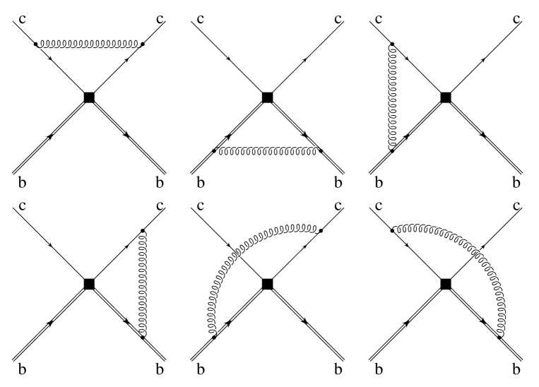
FIG. 5.: Diagrams which renormalize ${\cal O}_{1},\ldots,{\cal O}_{6}$.

The third class is those operators in which a derivative acts on the bottom quark. Here the classical equation of motion $v\cdot{\rm iD}h(x)=0$ eliminates some operators entirely. The remaining ones cannot mix directly with $\hat{m}^{4}\overline{h}\,h$ at order $\alpha_{s}^{0}$, but they can mix with the two other dimension seven operators we have identified so far. In $v\cdot A=0$ gauge, such mixing can only occur via the first two graphs in Fig. 6. Only color octet operators can mix with the color singlet $\overline{h}\,h\overline{c}\hbox to0.0pt{/\hss}vv\cdot{\rm iD}c$ by such one-gluon exchange. The operators in this class can also mix among themselves. However, it is straightforward to show that while color octets mix with both singlets and octets, color singlets mix only with each other. Hence, in this class of operators, only the color octets are relevant to our calculation. Furthermore, the Dirac structure is sufficiently constraining that of these, only $\overline{h}T_{a}{\rm iD}_{\mu}h\,\overline{c}T_{a}\gamma^{\mu}c$ contributes.

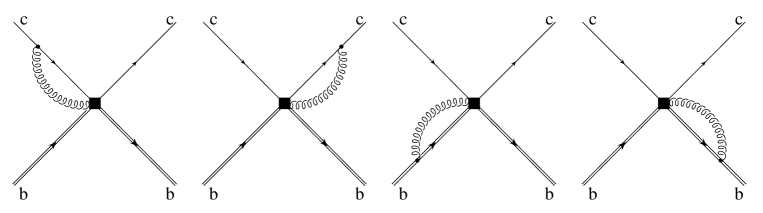
FIG. 6.: Additional diagrams which renormalize ${\cal O}_{3}$, ${\cal O}_{4}$ and ${\cal O}_{5}$.

There is one other source of dimension seven operators which we must consider. The HQET lagrangian beyond leading order is given by [18, 19]

$${\cal L}_{\rm HQET}=\overline{h}v\cdot{\rm iD}h+{1\over m_{b}}{\cal O}_{K}+{1\over m_{b}}C_{G}(\mu){\cal O}_{G}(\mu)+\dots\,,$$ (56)

where

$${\cal O}_{K}={1\over 2}\,\overline{h}({\rm iD})^{2}h\qquad{\rm and}\qquad{\cal O}_{G}={g\over 4}\,\overline{h}\sigma^{\mu\nu}G_{\mu\nu}h$$ (57)

are the leading spin and flavor symmetry violating corrections to the $m_{b}\to\infty$ limit. The operators ${\cal O}_{K}$ and ${\cal O}_{G}$ are treated as perturbations; because they come with explicit factors of $1/m_{b}$, they can induce mixing between operators at different order in the $1/m_{b}$ expansion [20]. In particular, they can mix operators of dimension six with those of dimension seven, via the graphs shown in Fig. 7. We find that insertions of ${\cal O}_{G}$ do not induce mixing with any of the dimension seven operators of interest, while ${\cal O}_{K}$ does, if the dimension six operator which is being renormalized is $\overline{h}T_{a}h\,\overline{c}\hbox to0.0pt{/\hss}vT_{a}c$.

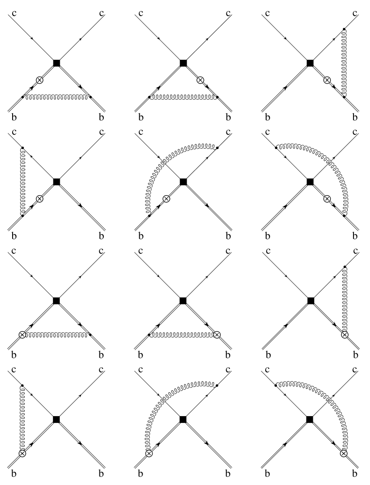
FIG. 7.: Diagrams with a single insertion of ${\cal O}_{K}$ mixing ${\cal O}_{1}$ with operators of dimension 7.

With this taxonomy in hand, we can now write down the list of operators of dimension six and seven which are relevant for our analysis. In the end, it is mercifully short:

$${\cal O}_{1} = \overline{h}T_{a}h\;\overline{c}\hbox to0.0pt{/\hss}vT_{a}c$$ (58)

$${\cal O}_{2} = \overline{h}T_{a}h\;\overline{q}_{i}\hbox to0.0pt{/\hss}vT_{a}q_{i}\,,\qquad q_{i}=u,\,d,\,s$$ (59)

$${\cal O}_{3} = {1\over 2m_{b}}\overline{h}\big{\{}{\rm-i}\overleftarrow{\rm D}\!_{\mu}T_{a}+T_{a}{\rm i}\overrightarrow{\rm D}\!_{\mu}\big{\}}h\;\overline{c}\gamma^{\mu}T_{a}c$$ (60)

$${\cal O}_{4} = {1\over 2m_{b}}\overline{h}\big{\{}{\rm-i}\overleftarrow{\rm D}\!_{\mu}T_{a}+T_{a}{\rm i}\overrightarrow{\rm D}\!_{\mu}\big{\}}h\;\overline{q}_{i}\gamma^{\mu}T_{a}q_{i}\,,\qquad q_{i}=u,\,d,\,s$$ (61)

$${\cal O}_{5} = {1\over 2m_{b}}\overline{h}\,h\;\overline{c}\hbox to0.0pt{/\hss}vv^{\mu}\big{\{}{\rm-i\overleftarrow{\rm D}}\!_{\mu}+{\rm i\overrightarrow{\rm D}}\!_{\mu}\big{\}}c$$ (62)

$${\cal O}_{6} = {m_{c}(\mu)\over m_{b}}\,\overline{h}\,h\;\overline{c}\,c$$ (63)

The operators ${\cal O}_{3}$, ${\cal O}_{4}$ and ${\cal O}_{5}$ have been constructed to be Hermitian. We also must include the quark bilinear $m_{c}^{4}\overline{h}\,h$. It is convenient to define it with an inverse factor of the strong coupling, because this will make the anomalous dimension matrix homogeneous in $g^{2}$:

$${\cal O}_{7}={1\over g^{2}(\mu)}\,{m_{c}^{4}(\mu)\over m_{b}}\,\overline{h}\,h\,.$$ (64)

Factors of $1/m_{b}$ have also been included in ${\cal O}_{3},\ldots,{\cal O}_{7}$ so that the anomalous dimension matrix will have no explicit factors of $1/m_{b}$. To summarize, the operators ${\cal O}_{1}$ through ${\cal O}_{6}$ are renormalized via the graphs in Fig. 5. In addition, the dimension seven operators ${\cal O}_{3},\ldots,{\cal O}_{6}$ get contributions from the graphs in Fig. 6. The dimension six operators ${\cal O}_{1}$ and ${\cal O}_{2}$ mix with each other via the “penguin” diagrams in Fig. 8, as do ${\cal O}_{3}$ and ${\cal O}_{4}$. Finally, ${\cal O}_{1}$ mixes with ${\cal O}_{5}$ and ${\cal O}_{6}$ via time-ordered products with ${\cal O}_{K}$, as shown in Fig. 7.

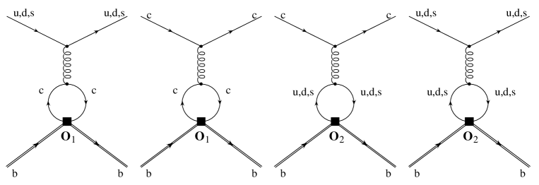
FIG. 8.: “Penguin” diagrams mixing ${\cal O}_{1}$ and ${\cal O}_{2}$. The same diagrams mix ${\cal O}_{3}$ and ${\cal O}_{4}$.

The operators in Eq. (58) are in fact not all independent; ${\cal O}_{1}$ and ${\cal O}_{3}$ (and ${\cal O}_{2}$ and ${\cal O}_{4}$) are related via reparameterization invariance[21]. Since $v_{\mu}$ and ${\rm D}_{\mu}$ must appear in the combination

$${\cal V}_{\mu}=v_{\mu}+i\overrightarrow{\rm D}_{\mu}/2m_{b}-i\overleftarrow{\rm D}_{\mu}/2m_{b}\,,$$ (65)

we find the restrictions

$$C_{1}(\mu)=C_{3}(\mu),\ \ C_{2}(\mu)=C_{4}(\mu)\,.$$ (66)

Our explicit calculations confirm this result.

We now perform the operator product expansion at the scale $\mu=m_{b}$. For the operators of dimension seven, the matching coefficients are generated at subleading order in the expansion in $1/m_{b}$. The momentum of the heavy $b$ quark is written as $p_{b}^{\mu}=m_{b}v^{\mu}+k^{\mu}$, where $k^{\mu}$ is the “residual” momentum. For an on-shell $h$ field, the classical equation of motion is $v\cdot k=0$ [8]. The expression of the $b$ quark spinor $u_{b}$ in terms of the heavy spinor $u_{h}$ is also affected, becoming $u_{b}=(1+\hbox to0.0pt{/\hss}k/2m_{b})u_{h}$ [18, 20, 22].

There are then two sources of matching onto operators of dimension seven. First, the lepton momentum $q^{\mu}$ may be written as $q^{\mu}=p_{b}^{\mu}-p_{c}^{\mu}=m_{b}v^{\mu}+k^{\mu}-p_{c}^{\mu}$. The momenta $k^{\mu}$ and $p_{c}^{\mu}$ lead to operators with covariant derivatives acting on the $h$ and $c$ fields, respectively. Second, the correction to the heavy quark spinors must be accounted for. We define reduced operator coefficients by

$$\hat{C}_{i}(\mu)={32\pi^{2}\over m_{b}^{3}}{\Gamma_{0}\over 2m_{B}}\,C_{i}(\mu)\,.$$ (67)

Then performing the operator product expansion at tree level yields the nonzero terms

$$\hat{C}_{1}(m_{b})=-3\,,\qquad\hat{C}_{3}(m_{b})=-3\,,\qquad\hat{C}_{5}(m_{b})={2\over 3}\,,\qquad\hat{C}_{6}(m_{b})={1\over 3}\,.$$ (68)

The Wilson coefficients evolve according the renormalization group equation

$$\mu{{\rm d}\over{\rm d}\mu}\hat{C}_{i}(\mu)=\gamma_{ji}\hat{C}_{j}(\mu)\,.$$ (69)

The anomalous dimension matrix $\gamma_{ij}$ is defined by the operator renormalization

$$\gamma_{ij}\Gamma^{(n)}_{{\cal O}_{j}}=-\left(\mu{\partial\over\partial\mu}+\beta{\partial\over\partial\beta}+\gamma_{m_{c}}m_{c}{\partial\over\partial m_{c}}-n\gamma_{\rm ext}\right)\Gamma^{(n)}_{{\cal O}_{i}}\,,$$ (70)

where $\Gamma^{(n)}_{{\cal O}_{i}}$ is an $n$-point Green function with a single insertion of the operator ${\cal O}_{i}$. Using the known mass and wavefunction anomalous dimensions [3, 4, 6, 11]

$$\gamma_{m_{c}}=-{g^{2}\over 2\pi^{2}}\,,\qquad\gamma_{c}={g^{2}\over 12\pi^{2}}\,,\qquad\gamma_{h}=-{g^{2}\over 6\pi^{2}}\,,$$ (71)

the Feynman diagrams in Figs. 4–8 yield the anomalous dimension matrix

$$\gamma_{ij}={g^{2}\over\pi^{2}}\left(\matrix{{-23/48}&{1/12}&0&0&-{2/9}&-{1/9}&0\cr{1/4}&-{5/16}&0&0&0&0&0\cr 0&0&{-23/48}&{1/12}&0&{1/6}&0\cr 0&0&{1/4}&-{5/16}&0&0&0&\cr 0&0&0&0&{4/9}&-{1/9}&-{3/8}\cr 0&0&0&0&0&0&-{3/2}\cr 0&0&0&0&0&0&{23/24}\cr}\right).$$ (72)

The renormalization group is then used to evolve the coefficients $\hat{C}_{i}(\mu)$ from $\mu=m_{b}$ to $\mu=m_{c}$. The logarithmically enhanced terms $\hat{m}_{c}^{4}\alpha_{s}^{n}\ln^{n+1}\hat{m}_{c}$ are given by the combination

$$F(m_{c})=C_{7}(m_{c})\,{m_{c}^{4}(m_{c})\over g^{2}(m_{c})m_{b}}\langle B|\,\overline{h}\,h\,|B\rangle={8\pi\over\alpha_{s}(m_{c})}\,\hat{m}_{c}^{4}\,\hat{C}_{7}(m_{c})\,{\Gamma_{0}\over 2m_{B}}\langle B|\,\overline{h}\,h\,|B\rangle\,.$$ (73)

By inspection of the matching coefficients (68) and the anomalous dimension matrix (72), we see that only the linear combination ${\cal O}_{5}-4{\cal O}_{6}$ mixes into ${\cal O}_{7}$, and that this linear combination of operators does not run in the leading logarithmic approximation. Therefore, the solution to the renormalization group equation for $\hat{C}_{7}(\mu)$ is particularly simple. With the matrix element (25), we find

$$F(m_{c})=\Gamma_{0}\,{8\pi\over\alpha_{s}(m_{c})}\,\hat{m}_{c}^{4}\,{18\over 23}\,(1-z^{-23/25})\,.$$ (74)

When expanded and written in terms of $\alpha_{s}(m_{b})$ and the reduced pole mass $\hat{m}_{c}$, the first two terms of the expression

$$\Gamma_{0}^{-1}\,F(m_{c}) = -24\hat{m}_{c}^{4}\ln\hat{m}_{c}-96{\alpha_{s}(m_{b})\over\pi}\,\hat{m}_{c}^{4}\ln^{2}\hat{m}_{c}+{32\over 3}\left({\alpha_{s}(m_{b})\over\pi}\right)^{2}\hat{m}_{c}^{4}\ln^{3}\hat{m}_{c}$$ (76)

$$\mbox{}-12\left({\alpha_{s}(m_{b})\over\pi}\right)^{3}\hat{m}_{c}^{4}\ln^{4}\hat{m}_{c}+{104\over 5}\left({\alpha_{s}(m_{b})\over\pi}\right)^{4}\hat{m}_{c}^{4}\ln^{5}\hat{m}_{c}+\dots\,,$$

reproduce the known tree level and one loop results from Eqs. (2) and (6), respectively. In addition, all of the leading logarithms have been resummed.

As in the previous section we use $\alpha_{s}(m_{c})=0.41$ and $\hat{m}_{c}=0.37$ to find

$$F(m_{c})=\Gamma_{0}\,[0.45-0.15-1.4\cdot 10^{-3}+\ldots]=\Gamma_{0}\,[0.30]$$ (77)

The re-expanded contributions from the terms $\hat{m}_{c}^{2}\overline{h}h$ and $\hat{m}_{c}^{3}\overline{h}h$ are

$${\Gamma_{0}\over 2m_{B}}\,\hat{m}_{c}^{2}(m_{b})\langle B|\,\overline{h}\,h\,|B\rangle=\Gamma_{0}\,[-1.10-0.37-0.12+\ldots]=\Gamma_{0}\,[-1.67]$$ (78)

and

$${\Gamma_{0}\over 2m_{B}}\,\hat{m}_{c}^{3}(m_{b})\langle B|\,\overline{h}\,h\,|B\rangle=\Gamma_{0}\,[\,0+0.92+0.46+\ldots]=\Gamma_{0}\,[1.71]$$ (79)

From these expansions, a large contribution at ${\cal O}(\alpha_{s}^{2}\hat{m}_{c}^{3}\ln\hat{m}_{c})$ can be seen. As discussed in the introduction, one can expect a cancelation of this term by the $\alpha_{s}^{2}\hat{m}_{c}^{4}\ln\hat{m}_{c}$ term, which has not been calculated here.

IV Summary

We have studied the operator product expansion for the process $b\to c\ell\bar{\nu}$, to understand better the origin of the “phase space” logarithms which appear in the total decay rate. After extracting the known tree level term, we have extended the analysis to include radiative corrections. In particular, we have used a renormalization group analysis to resum the leading logarithms of the form $\hat{m}_{c}^{2}\alpha_{s}^{n}\ln^{n}\hat{m}_{c}$, $\,\hat{m}_{c}^{3}\alpha_{s}^{n+1}\ln^{n}\hat{m}_{c}$ and $\,\hat{m}_{c}^{4}\alpha_{s}^{n}\ln^{n+1}\hat{m}_{c}$. Unfortunately, these terms do not dominate, in any limit of the theory, over certain others which have been omitted. Hence the results of this calculation cannot be used to extract any reasonable estimate of the true size of the higher order corrections.

The point of this calculation lies rather in the insight which it affords us into the origin of these logarithms, which even though not divergent, reflect sensitivity to physics which is far in the infrared with respect to the scale of the decaying $b$ quark. We have exploited this separation of scales to resum to all orders a certain subset of the phase space logarithms. In so doing, we have explored more generally their relation to other logarithms which appear in the theory, such as the “hybrid” anomalous dimensions of the heavy weak current [3, 4]. The hybrid anomalous dimensions are also not numerically dominant, but by studying them one may investigate interesting questions of principle in the Heavy Quark Effective Theory. The analysis and resummation which we have performed here should be viewed in much the same spirit.

REFERENCES

[1] Y. Nir, Phys. Lett. B221, 184 (1989).
[2] M. Luke, M.J. Savage and M.B. Wise, Phys. Lett. B343,
329 (1995); B345, 301 (1995).
[3] M. Voloshin and M. Shifman, Sov. J. Nucl. Phys. 45, 292 (1987); 47, 511 (1988).
[4] H.D. Politzer and M.B. Wise, Phys. Lett. B206, 681 (1988);
B208, 504 (1988).
[5] N. Isgur and M.B. Wise, Phys. Lett. B232, 113 (1989);
B237, 527 (1990).
[6] E. Eichten and B. Hill, Phys. Lett. B234, 511 (1990).
[7] B. Grinstein, Nucl. Phys. B339, 253 (1990).
[8] H. Georgi, Phys. Lett. B240, 447 (1990).
[9] J. Chay, H. Georgi and B. Grinstein, Phys. Lett. B247, 399 (1990).
[10] M. Shifman and M. Voloshin, Sov. J. Nucl. Phys.
41, 120 (1985).
[11] A.F. Falk, H. Georgi, B. Grinstein and M.B. Wise, Nucl. Phys. B343, 1 (1990).
[12] A.F. Falk and M. Neubert, Phys. Rev. D47, 2965 (1993).
[13] I.I. Bigi, N.G. Uraltsev and A.I. Vainshtein,
Phys. Lett. B293, 430 (1992); I.I. Bigi, M. Shifman, N.G. Uraltsev and
A.I. Vainshtein, Phys. Rev. Lett. 71, 496 (1993);
B. Blok, L. Koyrakh, M. Shifman and A.I. Vainshtein, Phys. Rev. D49, 3356 (1994) (Erratum, D50, 3572 (1994)).