BUTP–96/9
HUTP95/-A051
TTP96–02
hep-ph/9604279
April 1996

Tau Decays and Chiral Perturbation Theory
Gilberto Colangelo

Institut für Theoretische Physik
Universität Bern
Sidlerstrasse 5
CH-3012 Bern, Switzerland
Markus Finkemeier

Lyman Laboratory of Physics
Harvard University
Cambridge, MA 02138, USA
Res Urech

Institut für Theoretische Teilchenphysik
Universität Karlsruhe
D-76128 Karlsruhe, Germany
Abstract

In a small window of phase space, chiral perturbation theory can be used to make standard model predictions for tau decays into two and three pions. For $\displaystyle\tau\to 2\pi\nu_{\tau}$, we give the analytical result for the relevant form factor $\displaystyle F_{V}$ up to two loops, then calculate the differential spectrum and compare with available data. For $\displaystyle\tau\to 3\pi\nu_{\tau}$, we have calculated the hadronic matrix element to one loop. We discuss the decomposition of the three pion states into partition states and we give detailed predictions for the decay in terms of structure functions. We also compare with low energy predictions of meson dominance models. Overall, we find good agreement, but also some interesting discrepancies, which might have consequences beyond the limit of validity of chiral perturbation theory.

1 Introduction

Semileptonic decays of the heavy tau lepton into a tau neutrino and a hadronic system offer a unique laboratory to study the standard model and especially low energy QCD. A variety of multi-meson final states with invariant masses from the production threshold up to the tau mass of about $\displaystyle 1.8\,\mbox{GeV}$ can be studied. These final states can also be produced using hadronic initial states (such as pion-nucleon or nucleon-nucleon collisions). The production in tau decays, however, is advantageous in that the initial state is simple, clean and well understood. Whereas some of the final states (e.g. two or four pions) can also be produced using an electromagnetic current, i.e. electron-positron annihilation, other states (e.g. three pions in an $\displaystyle I=1$ state) can only be produced through the weak current. And in the case of the states which can be produced both in tau decays and in electron-positron annihilation, such as the two and four pion final states, tau days now compete well in statistics with electromagnetic production.

For inclusive semileptonic tau decays, the tau mass of about $\displaystyle 1.8\,\mbox{GeV}$ is large enough to allow the application of perturbative QCD and in fact offers a unique possibility to measure the strong coupling constant $\displaystyle\alpha_{s}(\mu)$ at the low scale $\displaystyle\mu=M_{\tau}$ [1]. In the case of exclusive semileptonic decays, calculations based on a systematic use of the QCD Lagrangian are not available up to now. In these decays, the probe testing the hadronic current carries a momentum $\displaystyle Q$ which is mainly in the intermediate energy region, the most difficult one for the study of strong interactions. In this region theoretical predictions have been obtained by using some kind of phenomenological models or approximate methods, such as quark models [2, 3], vector meson dominance [4, 5, 6, 7, 8, 9], tree level calculations from effective Lagrangians [10], or unitarization of current algebra results [11].

A small fraction of these decays, however, happens with very low $\displaystyle Q^{2}$, below the mass of the lightest resonance. In this region the only active fields are the pseudoscalar mesons and one can use an effective Lagrangian to describe their interactions. This effective theory, called Chiral Perturbation Theory (CHPT), is a systematic method to calculate QCD matrix elements at low energy by means of an expansion in powers of the external hadronic momenta [12, 13, 14].

The limits of applicability of CHPT do not allow to give predictions for integrated decay rates, which would involve $\displaystyle Q^{2}$ up to $\displaystyle M_{\tau}^{2}$. Furthermore, tau decays into more than a single pion are dominated by resonant intermediate states, such as the $\displaystyle\rho(770)$ in the two pion channel and the $\displaystyle a_{1}(1260)$ in the three pion channel. And so there are only relatively few events with small $\displaystyle Q^{2}$. For these reasons, in the past, CHPT has been considered as not very interesting for tau decays.

However, with the present high luminosity machines such as LEP and CESR, and even more so with future b and perhaps tau-charm factories, tau physics has turned into an era of precision measurements, exploring very small branching ratios and studying details of differential distributions. Thus the small $\displaystyle Q^{2}$ regime which is interesting for CHPT is now becoming accessible.

We would like to mention that there is another small corner of phase space where a different systematic expansion of the hadronic current becomes possible. Heavy meson chiral perturbation theory [15] can be applied to tau decays into a vector meson and a pion (such as $\displaystyle\tau\to\rho\pi\nu_{\tau}$, $\displaystyle\tau\to K^{*}\pi\nu_{\tau}$), if the momentum of the pion is small in the vector meson rest frame [16]. A complete calculation which includes vector meson decay and interference effects between different vector meson amplitudes, however, is still missing in this approach.

Another reason why CHPT is relevant to tau decays is the fact that it can be used to test phenomenological models or fix some of their parameters. Indeed, the $\displaystyle O(p^{2})$ prediction of CHPT in the limit of vanishing quark masses has been used to normalize vector meson dominance models in [4, 5, 7, 8, 9]. In the present paper we will extend the CHPT prediction to higher order in $\displaystyle p^{2}$, and it will be a severe test for models if they correctly reproduce these higher orders.

The expansion parameter of CHPT is $\displaystyle Q^{2}/(4\pi F_{\pi})^{2}$, with $\displaystyle 4\pi F_{\pi}=1.2\,\mbox{GeV}$, so we are interested in $\displaystyle\sqrt{Q^{2}}$ below $\displaystyle 500\dots 600\,\mbox{MeV}$. Hadronic final states with a single pion or kaon can be predicted directly from $\displaystyle F_{\pi}$ and $\displaystyle F_{K}$ [17], and so there is nothing interesting CHPT could teach us here. Final states with two and three pions allow for a reasonably large region of $\displaystyle Q^{2}$ between threshold and the limit of applicability of CHPT. Already with four pions this region has almost disappeared. Moreover, the phase space for a $\displaystyle n$ pion hadronic state, with $\displaystyle Q^{2}$ close to threshold $\displaystyle Q^{2}\to(nM_{\pi})^{2}$, opens proportional to

$$\Big{(}\sqrt{Q^{2}}-nM_{\pi}\Big{)}^{(3n-5)/2}$$ (1)

(see Sec. 3.1 below). The exponent is $\displaystyle 1/2$ for two pions, $\displaystyle 2$ for three pions and $\displaystyle 7/2$ for four pions. So in the case of four pions the small interesting region for CHPT is even more suppressed by the phase space. As for final states with kaons, the threshold for a pion-kaon state is $\displaystyle M_{\pi}+M_{K}=634\,\mbox{MeV}$ . Furthermore the $\displaystyle K^{*}(892)$ resonance is very close [18].

Therefore we find reasonable to try a CHPT calculation only for the $\displaystyle 2\pi$ and $\displaystyle 3\pi$ final states and these are the ones we will discuss in this paper. The two pion state is determined by only one form factor, namely the vector pion form factor. This can be measured in a few other processes, like $\displaystyle e^{+}e^{-}\to 2\pi$ or $\displaystyle\pi e$ scattering. Tau decays can provide an interesting cross check measurement, and we will investigate whether tau decays may become competitive in statistics. The three pion state, however, can only be produced in tau decay, and has a very rich and interesting substructure, which we will study in detail.

Our paper is organized as follows: A brief review of chiral perturbation theory is given in Sec. 2. In Sec. 3, we discuss the general structure of the phase space, the hadronic matrix element for two and three pions, and the differential decay rate. In this section we also discuss general properties of the three pion final state, regarding isospin invariance, the classification in terms of partition states and the definition of structure functions. We then calculate the hadronic matrix elements in CHPT in Sec. 4. Sec. 5 is dedicated to our numerical results, and in Sec. 6 we state our conclusions. In the Appendix we summarize our main conventions, display the decomposition of the three pion form factors into partition states and collect the main formulae regarding the definition of the structure functions.

2 Chiral Perturbation Theory

The relevant matrix elements for $\displaystyle\tau$ decays into pions are of the form:

$$\langle\pi^{i_{1}}(p_{1})\ldots\pi^{i_{n}}(p_{n}){\rm out}|I^{k}_{\mu}(0)|0\rangle$$ (2)

where $\displaystyle I^{k}_{\mu}=V^{k}_{\mu}=\frac{1}{2}\bar{q}\tau^{k}\gamma_{\mu}q$ when $\displaystyle n$ is even, and $\displaystyle I^{k}_{\mu}=A^{k}_{\mu}=\frac{1}{2}\bar{q}\tau^{k}\gamma_{\mu}\gamma_{5}q$ when $\displaystyle n$ is odd. A by now standard method to calculate such matrix elements in QCD at low energy is Chiral Perturbation Theory, CHPT. In this framework one uses an effective Lagrangian that respects the chiral symmetry properties of QCD, and that has the pions as the only “active” fields. Of course this Lagrangian is expected to be valid only up to energies which are well below the threshold for the production of heavier hadronic states. For more details about this method we refer the reader to the fundamental paper by Gasser and Leutwyler [13] and to a number of excellent reviews which are presently available in the literature [14]. Here we simply sketch the basic ideas and introduce the relevant notation.

We consider the effective Lagrangian relative to two flavors in the isospin limit $\displaystyle\hat{m}=m_{u}=m_{d}$. This Lagrangian contains an infinite number of terms; however it can be expanded in powers of derivatives and quark masses. One power of the quark mass will be counted as two powers of derivatives. One will then have:

$${\cal L}_{\rm eff}={\cal L}_{2}+\hbar{\cal L}_{4}+\hbar^{2}{\cal L}_{6}+\ldots\;.$$ (3)

The leading order Lagrangian starts at $\displaystyle O(p^{2})$ and is the nonlinear $\displaystyle\sigma$-model Lagrangian in the presence of external fields, which we represent here in matrix form, $\displaystyle a_{\mu}=a^{k}_{\mu}\tau^{k}$, $\displaystyle v_{\mu}=v^{k}_{\mu}\tau^{k}$:

$$\displaystyle{\cal L}_{2} \displaystyle= \displaystyle\frac{F^{2}}{4}\langle D^{\mu}UD_{\mu}U^{\dagger}+M^{2}\left(U+U^{\dagger}\right)\rangle$$

$$\displaystyle D_{\mu}U \displaystyle= \displaystyle\partial_{\mu}U-i(v_{\mu}+a_{\mu})U+iU(v_{\mu}-a_{\mu})$$

$$\displaystyle M_{\pi}^{2} \displaystyle= \displaystyle M^{2}\left[1+O(\hat{m})\right]$$

$$\displaystyle M^{2} \displaystyle= \displaystyle 2B\hat{m}$$

$$\displaystyle F_{\pi} \displaystyle= \displaystyle F\left[1+O(\hat{m})\right]$$ (4)

$\displaystyle B$ is proportional to the quark condensate $\displaystyle\langle 0|\bar{u}u|0\rangle$ and the unitary $\displaystyle 2\times 2$ matrix $\displaystyle U$ contains the pion fields,

$$\displaystyle U \displaystyle= \displaystyle\sigma+i\frac{\phi}{F}\hskip 56.9055pt\sigma^{2}+\frac{\phi^{2}}{F^{2}}={\bf 1}$$

$$\displaystyle\phi \displaystyle= \displaystyle\left(\begin{array}[]{cc}\pi^{0}&\sqrt{2}\pi^{+}\\ \sqrt{2}\pi^{-}&-\pi^{0}\end{array}\right)\;\;.$$ (7)

The external fields $\displaystyle v^{k}_{\mu}$ and $\displaystyle a^{k}_{\mu}$, which we have introduced, have to be treated as external sources for the quark currents $\displaystyle V^{k}_{\mu}$ and $\displaystyle A^{k}_{\mu}$ respectively; in other words, the currents coupled to $\displaystyle v^{k}_{\mu}$ and $\displaystyle a^{k}_{\mu}$ in the effective Lagrangian are the low energy representation of the quark currents. In this framework these currents are expanded in powers of derivatives and quark masses, and are nonlinear in the pion fields, e.g. the axial vector current,

$$A_{\mu}^{k}=\frac{iF^{2}}{4}\langle\tau^{k}(U^{\dagger}D_{\mu}U-UD_{\mu}U^{\dagger})\rangle+O(p^{3})=\left[-F\partial_{\mu}\phi^{k}+O(\phi^{3})\right]+O(p^{3})\;\;.$$ (8)

Despite the fact that this Lagrangian is nonrenormalizable, one can use it to calculate matrix elements with the standard perturbation theory. As we have emphasized in Eq. (2) the expansion parameter is $\displaystyle\hbar$. This automatically produces an expansion of the matrix elements in powers of momenta and quark masses. As for the matrix elements in question, tree diagrams from $\displaystyle{\cal L}_{2}$ generate leading order contributions [4, 5, 7, 8], while one-loop diagrams yield terms at next-to-leading order. The occurring divergences in the loop contributions (in $\displaystyle d=4$ dimensions) can be absorbed by introducing the effective Lagrangian at $\displaystyle O(p^{4})$ [13],

$$\displaystyle{\cal L}_{4} \displaystyle= \displaystyle\frac{1}{4}l_{1}\langle D^{\mu}UD_{\mu}U^{\dagger}\rangle^{2}+\frac{1}{4}l_{2}\langle D_{\mu}UD_{\nu}U^{\dagger}\rangle\langle D^{\mu}UD^{\nu}U^{\dagger}\rangle$$

$$\displaystyle+\frac{1}{16}l_{3}M^{4}\langle U+U^{\dagger}\rangle^{2}+\frac{i}{2}l_{4}M^{2}\langle a_{\mu}\left(D^{\mu}U-D^{\mu}U^{\dagger}\right)\rangle$$

$$\displaystyle+l_{5}\langle F_{R}^{\mu\nu}UF_{L\;\mu\nu}U^{\dagger}\rangle+\frac{i}{2}l_{6}\langle F_{R}^{\mu\nu}D_{\mu}UD_{\nu}U^{\dagger}+F_{L}^{\mu\nu}D_{\mu}U^{\dagger}D_{\nu}U\rangle+\ldots$$

$$\displaystyle F_{R,L}^{\mu\nu} \displaystyle= \displaystyle\partial^{\mu}(v^{\nu}\pm a^{\nu})-\partial^{\nu}(v^{\mu}\pm a^{\mu})-i[v^{\mu}\pm a^{\mu},v^{\mu}\pm a^{\mu}]$$ (9)

where we omitted terms which contain external fields only. Since we disregard singlet vector and axial vector currents (i.e. $\displaystyle\langle v_{\mu}\rangle=\langle a_{\mu}\rangle=0$) there is no contribution from the anomaly at $\displaystyle O(p^{4})$ [13].

The coupling constants $\displaystyle l_{i}$ are split in a divergent and a finite piece and are scale-independent by definition,

$$\displaystyle l_{i} \displaystyle= \displaystyle\gamma_{i}\lambda+l_{i}^{r}(\mu),\hskip 56.9055pt\lambda=\frac{\mu^{d-4}}{16\pi^{2}}\left\{\frac{1}{d-4}-\frac{1}{2}[\ln 4\pi+\Gamma^{\prime}(1)+1]\right\}$$

$$\displaystyle\mu\frac{d}{d\mu}l_{i} \displaystyle= \displaystyle\gamma_{i}\frac{\mu^{d-4}}{16\pi^{2}}+\mu\frac{d}{d\mu}l_{i}^{r}(\mu)+O(d-4)=0$$ (10)

The finite parts have been determined phenomenologically for the first time by Gasser and Leutwyler [13]. We adopt their notation and use instead of the $\displaystyle l_{i}^{r}(\mu)$, the finite and scale-independent quantities $\displaystyle\bar{l}_{i}$,

$$\bar{l}_{i}=\left(\frac{\gamma_{i}}{32\pi^{2}}\right)^{-1}l_{i}^{r}(\mu)\;-\;\ln\frac{M^{2}}{\mu^{2}}$$ (11)

The up to date values for the relevant $\displaystyle\bar{l}_{i}$ and the corresponding $\displaystyle\gamma_{i}$ are listed in Table 1.

$\displaystyle i$	$\displaystyle\hskip 14.22636pt\bar{l}_{i}$	$\displaystyle\gamma_{i}$
1	$\displaystyle-1.7$ $\displaystyle\pm$ 1.0	1/3
2	6.1 $\displaystyle\pm$ 0.5	2/3
3	2.9 $\displaystyle\pm$ 2.4	$\displaystyle-1/2$
4	4.3 $\displaystyle\pm$ 0.9	2
6	16.5 $\displaystyle\pm$ 1.1	$\displaystyle-1/3$

Table 1: The set of $\displaystyle\bar{l}_{i}$ and corresponding $\displaystyle\gamma_{i}$ which we need for the calculation of the matrix elements in question. The values are taken from [20] for $\displaystyle i=1,2$, and from [13] for all the others. The $\displaystyle\gamma_{i}$ determine the relation between the $\displaystyle\bar{l_{i}}$ and the $\displaystyle l^{r}_{i}(\mu)$.

For completeness we give the expressions for the pion decay constant and the pion mass up to and including $\displaystyle O(p^{4})$,

$$\displaystyle F_{\pi} \displaystyle= \displaystyle F\left[1+\frac{M^{2}}{16\pi^{2}F^{2}}\bar{l}_{4}+O(M^{4})\right]$$

$$\displaystyle M_{\pi}^{2} \displaystyle= \displaystyle M^{2}\left[1-\frac{M^{2}}{32\pi^{2}F^{2}}\bar{l}_{3}+O(M^{4})\right]$$ (12)

The mass splitting $\displaystyle M_{\pi^{\pm}}^{2}-M_{\pi^{0}}^{2}$ is proportional to $\displaystyle(m_{u}-m_{d})^{2}$ and thus may be neglected. In the numerical evaluation, we will use $\displaystyle M_{\pi}=139.57\,\mbox{MeV}$ and $\displaystyle F_{\pi}=93.1\,\mbox{MeV}$.

If one wants to go beyond the next-to-leading order, one has to calculate two loop diagrams with $\displaystyle{\cal L}_{2}$, and one loop diagrams with one vertex from $\displaystyle{\cal L}_{4}$. Again these diagrams will be divergent, but this is not a problem since at the same order one has contributions from tree diagrams with the $\displaystyle{\cal L}_{6}$ Lagrangian (which has been constructed in the case of three lights flavors [21]). By defining appropriately the new coupling constants occurring in this Lagrangian, one is able to remove the divergences at the next–to–next–to–leading order, and get finite matrix elements. In order to have numerical predictions at this level one has to find a way to pin down or at least to estimate the finite parts of the new low energy constants. At the moment this has not been done yet in a systematic way: in Sec. 4.1, when calculating the matrix element of the $\displaystyle\tau$ decay into two pions to two loops, we will show how in a specific case one can try to circumvent this problem.

3 Phase Space, Matrix Elements and Structure Functions

3.1 Phase Space Considerations

The two-pion phase space is given by

$$\Phi_{2\pi}=\frac{M_{\tau}^{2}}{128\pi^{3}}\int\frac{dQ^{2}}{M_{\tau}^{2}}\left(1-\frac{Q^{2}}{M_{\tau}^{2}}\right)\left(1-\frac{4M_{\pi}^{2}}{Q^{2}}\right)^{1/2}$$ (13)

(the reader is referred to App. A.1 for our conventions) where the integral is from threshold $\displaystyle 4M_{\pi}^{2}$ up to $\displaystyle M_{\tau}^{2}$. Close to the two pion threshold, this implies

$$\frac{d\Phi_{2\pi}}{dQ^{2}}\to\frac{1}{128\pi^{3}}\frac{1}{M_{\pi}^{1/2}}\left(1-\frac{4M_{\pi}^{2}}{M_{\tau}^{2}}\right)\Big{(}\sqrt{Q^{2}}-2M_{\pi}\Big{)}^{1/2}$$ (14)

The three pion phase space is

$$\displaystyle\Phi_{3\pi} \displaystyle= \displaystyle\frac{M_{\tau}^{2}}{2048\pi^{5}}\int_{9M_{\pi}^{2}}^{M_{\tau}^{2}}\frac{dQ^{2}}{M_{\tau}^{2}}\left(1-\frac{Q^{2}}{M_{\tau}^{2}}\right)\frac{1}{Q^{2}}\int_{4M_{\pi}^{2}}^{(\sqrt{Q^{2}}-M_{\pi})^{2}}\frac{ds_{1}}{s_{1}}$$ (15)

$$\displaystyle\quad\times[(s_{1}-Q^{2}-M_{\pi}^{2})^{2}-4Q^{2}M_{\pi}^{2}]^{1/2}[s_{1}(s_{1}-4M_{\pi}^{2})]^{1/2}$$

Close to threshold $\displaystyle Q^{2}\to 9M_{\pi}^{2}$ this can be approximated by

$$\frac{d\Phi_{3\pi}}{dQ^{2}}\to\frac{1}{2^{10}3^{3/2}\pi^{4}}\left(1-\frac{9M_{\pi}^{2}}{M_{\tau}^{2}}\right)\Big{(}\sqrt{Q^{2}}-3M_{\pi}\Big{)}^{2}$$ (16)

By induction we can show [23] that the phase space for a $\displaystyle n$ pion hadronic state, with $\displaystyle Q^{2}$ close to threshold, $\displaystyle Q^{2}\to(nM_{\pi})^{2}$, opens proportional to:

$$\frac{d\Phi_{n\pi}}{dQ^{2}}\propto\Big{(}\sqrt{Q^{2}}-nM_{\pi}\Big{)}^{(3n-5)/2}$$ (17)

For $\displaystyle n=2$, the exponent is $\displaystyle 1/2$, for $\displaystyle n=3$ it is $\displaystyle 2$, recovering the above results.

It is clear that in general, the more pions there are, the slower the phase space opens at threshold. Therefore for four and more pions, it is not only the high invariant hadronic mass, but also the behavior of the phase space at threshold which prevents the application of CHPT.

3.2 Two Pion Differential Decay Rate

The hadronic matrix element of the decay into two pions is characterized by a single form factor, $\displaystyle F_{V}(Q^{2})$,

$$H^{\mu}=\langle\pi^{-}(p_{1})\pi^{0}(p_{2})|V^{\mu}-A^{\mu}|0\rangle=\sqrt{2}(p_{1}-p_{2})^{\mu}F_{V}\left(Q^{2}\right)$$ (18)

Only $\displaystyle|F_{V}(Q^{2})|$ can be measured, and it can be obtained by measuring the differential distribution in $\displaystyle Q^{2}$ using

$$\frac{d\Gamma_{2\pi}}{\Gamma_{e}}(Q^{2})=\frac{\cos^{2}\theta_{c}}{2}\frac{dQ^{2}}{M_{\tau}^{2}}\left(1-\frac{Q^{2}}{M_{\tau}^{2}}\right)^{2}\left(1+\frac{2Q^{2}}{M_{\tau}^{2}}\right)\left(1-\frac{4M_{\pi}^{2}}{Q^{2}}\right)^{3/2}|F_{V}(Q^{2})|^{2}$$ (19)

Here we have normalized to the electronic branching ratio of the tau:

$$\Gamma_{e}=\frac{G_{F}^{2}M_{\tau}^{5}}{192\pi^{3}}$$ (20)

3.3 Structure Functions and the Three Pion Differential Decay Rate

3.3.1 Form Factors and Isospin Relations

The most general form of the hadronic matrix elements for the tau decays into the $\displaystyle 2\pi^{-}\pi^{+}$ and $\displaystyle 2\pi^{0}\pi^{-}$ final states, compatible with the requirements of Lorentz, isospin and $\displaystyle G$ parity invariance and Bose symmetry is given in terms of three functions $\displaystyle F,\;G$ and $\displaystyle H$ which have to satisfy the following property:

$$\displaystyle F(s_{2},s_{1},s_{3}) \displaystyle= \displaystyle+F(s_{1},s_{2},s_{3})$$

$$\displaystyle G(s_{2},s_{1},s_{3}) \displaystyle= \displaystyle+G(s_{1},s_{2},s_{3})$$

$$\displaystyle H(s_{2},s_{1},s_{3}) \displaystyle= \displaystyle-H(s_{1},s_{2},s_{3})\;.$$ (21)

The matrix elements are then given by

$$\displaystyle\langle\pi^{0}(p_{1})\pi^{0}(p_{2})\pi^{-}(p_{3})|A_{\mu}^{-}(0)|0\rangle$$ (22)

$$\displaystyle= \displaystyle G(s_{1},s_{2},s_{3})(p_{1}+p_{2})_{\mu}+H(s_{1},s_{2},s_{3})(p_{1}-p_{2})_{\mu}+F(s_{1},s_{2},s_{3})p_{3\,\mu}$$

$$\displaystyle\langle\pi^{-}(p_{1})\pi^{-}(p_{2})\pi^{+}(p_{3})|A_{\mu}^{-}(0)|0\rangle$$

$$\displaystyle= \displaystyle G^{(+)}(s_{1},s_{2},s_{3})(p_{1}+p_{2})_{\mu}+H^{(+)}(s_{1},s_{2},s_{3})(p_{1}-p_{2})_{\mu}+F^{(+)}(s_{1},s_{2},s_{3})p_{3\,\mu}\;.$$

The form factors for $\displaystyle 2\pi^{-}\pi^{+}$ and $\displaystyle 2\pi^{0}\pi^{-}$ are related by isospin symmetry

$$\displaystyle F^{(+)}(s_{1},s_{2},s_{3}) \displaystyle= \displaystyle\left[G(s_{2},s_{3},s_{1})+G(s_{3},s_{1},s_{2})-H(s_{2},s_{3},s_{1})+H(s_{3},s_{1},s_{2})\right]$$

$$\displaystyle G^{(+)}(s_{1},s_{2},s_{3}) \displaystyle= \displaystyle\frac{1}{2}\left[F(s_{2},s_{3},s_{1})+F(s_{3},s_{1},s_{2})+G(s_{2},s_{3},s_{1})+G(s_{3},s_{1},s_{2})\right.$$

$$\displaystyle\left.\hskip 28.45274pt+H(s_{2},s_{3},s_{1})-H(s_{3},s_{1},s_{2})\right]$$

$$\displaystyle H^{(+)}(s_{1},s_{2},s_{3}) \displaystyle= \displaystyle\frac{1}{2}\left[F(s_{2},s_{3},s_{1})-F(s_{3},s_{1},s_{2})-G(s_{2},s_{3},s_{1})+G(s_{3},s_{1},s_{2})\right.$$ (23)

$$\displaystyle\left.\hskip 28.45274pt-H(s_{2},s_{3},s_{1})-H(s_{3},s_{1},s_{2})\right]$$

Alternatively one can use a decomposition of the matrix element into only two functions, $\displaystyle F_{1}(s_{1},s_{2},s_{3})$ and $\displaystyle F_{S}(s_{1},s_{2},s_{3})$, with $\displaystyle F_{S}$ even under the exchange of the first two arguments, and $\displaystyle F_{1}$ of mixed behavior:

$$\displaystyle\langle\pi^{0}(p_{1})\pi^{0}(p_{2})\pi^{-}(p_{3})|A_{\mu}^{-}(0)|0\rangle$$

$$\displaystyle= \displaystyle[F_{1}(s_{1},s_{2},s_{3})(p_{1}-p_{3})^{\nu}+F_{1}(s_{2},s_{1},s_{3})(p_{2}-p_{3})^{\nu}]T_{\mu\nu}+F_{S}Q_{\mu}$$

$$\displaystyle\langle\pi^{-}(p_{1})\pi^{-}(p_{2})\pi^{+}(p_{3})|A_{\mu}^{-}(0)|0\rangle$$ (24)

$$\displaystyle= \displaystyle[F_{1}^{(+)}(s_{1},s_{2},s_{3})(p_{1}-p_{3})^{\nu}+F_{1}^{(+)}(s_{2},s_{1},s_{3})(p_{2}-p_{3})^{\nu}]T_{\mu\nu}+F_{S}^{(+)}Q_{\mu}\;,$$

where

$$\displaystyle T_{\mu\nu} \displaystyle= \displaystyle g_{\mu\nu}-\frac{Q_{\mu}Q_{\nu}}{Q^{2}}$$

$$\displaystyle Q_{\mu} \displaystyle= \displaystyle(p_{1}+p_{2}+p_{3})_{\mu}$$

$$\displaystyle Q^{2} \displaystyle= \displaystyle s_{1}+s_{2}+s_{3}-3M_{\pi}^{2}\;.$$ (25)

The decomposition into $\displaystyle F_{1}$ and $\displaystyle F_{S}$ has the advantage that these form factors correspond to a definite overall spin (viz. $\displaystyle F_{1}$ corresponds to spin 1 and $\displaystyle F_{S}$ to spin 0), and therefore the structure functions (see next Sec. 4.2) are usually expressed through $\displaystyle F_{1}$ and $\displaystyle F_{S}$. If $\displaystyle F$, $\displaystyle G$ and $\displaystyle H$ are known, we can calculate $\displaystyle F_{1}$, $\displaystyle F_{S}$ through

$$\displaystyle F_{1}(Q^{2},s_{1},s_{2}) \displaystyle= \displaystyle\frac{-F(s_{1},s_{2},s_{3})+G(s_{1},s_{2},s_{3})}{3}+H(s_{1},s_{2},s_{3})$$

$$\displaystyle F_{S}(Q^{2},s_{1},s_{2}) \displaystyle= \displaystyle\alpha F(s_{1},s_{2},s_{3})+(1-\alpha)G(s_{1},s_{2},s_{3})-\beta H(s_{1},s_{2},s_{3})$$

$$\displaystyle\alpha \displaystyle= \displaystyle\frac{s_{1}+s_{2}-2M_{\pi}^{2}}{2Q^{2}}$$

$$\displaystyle\beta \displaystyle= \displaystyle\frac{s_{1}-s_{2}}{2Q^{2}}\;.$$ (26)

A completely analogous relation holds for the form factors of the all charged matrix element.

Let us emphasize two facts regarding the two charge modes. Firstly, the two matrix elements for the final states $\displaystyle 2\pi^{-}\pi^{+}$ and $\displaystyle 2\pi^{0}\pi^{-}$ are not independent. If one knows the matrix element for one of the two states, the other one can be calculated using isospin symmetry. Secondly, however, isospin symmetry does not require that the form factors and decay rates are equal for the two modes. This fact can be seen if we decompose the three pion states in terms of partitions [24].

3.3.2 Classification in Terms of Partitions

In Ref. [24], Pais introduced a classification of $\displaystyle N$ pion states with overall isospin $\displaystyle I=0$ or $\displaystyle 1$ in terms of correlation quantum numbers $\displaystyle[N_{1}N_{2}N_{3}]$. The three integer quantum numbers $\displaystyle N_{i}$ are partitions of the total number of pions $\displaystyle N$

$$\displaystyle N_{1}\geq N_{2}\geq N_{3}\geq 0$$

$$\displaystyle N_{1}+N_{2}+N_{3}=N$$ (27)

Each state $\displaystyle[N_{1}N_{2}N_{3}]$ is characterized by its symmetry property under the exchange of some of the momenta $\displaystyle p_{1},\ldots,p_{N}$. Such a state is easily constructed with the help of a Young tableau: each Young diagram must have three rows with $\displaystyle N_{1},\;N_{2}$ and $\displaystyle N_{3}$ cells in the first, second and third row, respectively. The cells must then be filled with numbers going from 1 to $\displaystyle N$, with the only rule that all the numbers in the rows (columns) must be organized in increasing order from left to right (top to bottom). The rule to construct a pion state from a tableau is very simple: one has to symmetrize with respect to the exchange of the momenta with the indices which are in a row, and antisymmetrize with respect to the momenta with the indices which are in a column. The order of these operations of symmetrization or antisymmetrization is not important, but must be fixed once and for all.

Remarkably, all the states belonging to the same class defined by the partition $\displaystyle[N_{1}N_{2}N_{3}]$ share some common properties about isospin and charge distributions:

1. the overall isospin $\displaystyle I$ is uniquely determined and it is $\displaystyle I=0$ if $\displaystyle N_{1}-N_{3}$ and $\displaystyle N_{2}-N_{3}$ are both even, and $\displaystyle I=1$ otherwise;

2. the states in a class $\displaystyle[N_{1}N_{2}N_{3}]$ are composed by $\displaystyle N_{3}$ subsystems of three pions with $\displaystyle I=0$ and $\displaystyle N_{2}-N_{3}$ subsystems of two pions with $\displaystyle I=1$, and $\displaystyle N_{1}-N_{2}$ remaining single pions (trivially $\displaystyle 3N_{3}+2(N_{2}-N_{3})+(N_{1}-N_{2})=N$);

3. the $\displaystyle N$ pion states which we are describing contain all possible charge distributions (e.g. for $\displaystyle N=2$ and zero total charge, they would contain both $\displaystyle\pi^{+}\pi^{-}$ and $\displaystyle\pi^{0}\pi^{0}$ states). The probability of a state to contain a given charge distribution is a “class property”, i.e. is uniquely determined by the partition $\displaystyle[N_{1}N_{2}N_{3}]$ to which it belongs.

For a more detailed account of the properties of these $\displaystyle N$ pion states we refer the reader to the original article by Pais [24]. We now concentrate on the case of our interest $\displaystyle N=3$.

In this case we have three possible partitions: $\displaystyle[300]$, $\displaystyle[210]$ and $\displaystyle[111]$. The $\displaystyle[111]$ corresponds to $\displaystyle\pi^{+}\pi^{0}\pi^{-}$ in an overall $\displaystyle I=0$ state (e.g. from the decay $\displaystyle\omega\to 3\pi$). The remaining two partitions $\displaystyle[210]$ and $\displaystyle[300]$ have $\displaystyle I=1$ and so they can occur in $\displaystyle\tau\to 3\pi\nu_{\tau}$.

These two partitions differ in their branching ratios into the two charge distribution states. The $\displaystyle[210]$ decays equally into $\displaystyle 2\pi^{-}\pi^{+}$ and $\displaystyle 2\pi^{0}\pi^{-}$:

$$[210]:\qquad\frac{\mbox{BR}(2\pi^{-}\pi^{+})}{\mbox{BR}(2\pi^{0}\pi^{-})}=1$$ (28)

whereas the $\displaystyle[300]$ state prefers the all charged mode

$$[300]:\qquad\frac{\mbox{BR}(2\pi^{-}\pi^{+})}{\mbox{BR}(2\pi^{0}\pi^{-})}=4$$ (29)

(28,29) immediately lead to the inequalities obtained in Ref. [25]:

$$\frac{1}{5}\leq\frac{\mbox{BR}(2\pi^{0}\pi^{-})}{\mbox{BR}(\mbox{all}\;(3\pi)^{-})}\leq\frac{1}{2}\;,\;\;\qquad\frac{1}{2}\leq\frac{\mbox{BR}(2\pi^{-}\pi^{+})}{\mbox{BR}(\mbox{all}\;(3\pi)^{-})}\leq\frac{4}{5}\;.$$

Experimentally, the branching ratios of the $\displaystyle\tau$ into the two states are equal within the errors, so that certainly the $\displaystyle[210]$ strongly dominates and a possible small admixture of the $\displaystyle[300]$ state (which, as we will show below, is required by CHPT), has not yet been established. Note that if the decay occurs only via a decay chain $\displaystyle\tau\to a_{1}\nu_{\tau}$, $\displaystyle a_{1}\to\rho\pi$ and $\displaystyle\rho\to\pi\pi$, as in vector meson dominance models, there is only the $\displaystyle[210]$ state (because of the $\displaystyle\rho$ resonance, there is one two-pion subsystem with $\displaystyle I=1$, i.e. $\displaystyle N_{2}-N_{3}=1$), and both decay charge modes are produced with equal rates.

If one has an analytic expression for the form factors in each of the two charge modes, one can easily construct the matrix element of a given partition state, by following the rules which we described above. The complete decomposition of each of the form factors $\displaystyle F,\;G$ and $\displaystyle H$ into the three partition states (two states for the partition $\displaystyle[210]$ and one for $\displaystyle[300]$) is described in App. A.2. Here we give in an obvious notation the decomposition only of $\displaystyle F_{1}$, since it is the most important form factor in the numerical analysis:

$$\displaystyle F_{1} \displaystyle= \displaystyle\left[F_{1}^{[300]}+F_{1}^{[210]}\right]$$

$$\displaystyle F_{1}^{(+)} \displaystyle= \displaystyle\left[2F_{1}^{[300]}-F_{1}^{[210]}\right]\;,$$ (30)

where with $\displaystyle F_{1}^{[210]}$ we have indicated the sum of the two states belonging to the $\displaystyle[210]$ class. From this decomposition the branching ratios given in Eqs. (28,29) follow, and since $\displaystyle F_{1}^{\mbox{\tiny{VMD}}}=-F_{1}^{(+)\;\mbox{\tiny{VMD}}}$, it is clear that the $\displaystyle[300]$ partition is absent in the VMD model.

3.3.3 Structure Functions and Differential Decay Rate

The differential decay rate for a general hadronic decay is determined by

$$d\Gamma(\tau\to 3\pi\nu_{\tau})=\frac{G_{F}^{2}}{4M_{\tau}}\cos^{2}\theta_{C}L_{\mu\nu}H^{\mu\nu}\,dPS^{(4)}$$ (31)

where the hadronic and leptonic tensors are

$$L_{\mu\nu}:=L_{\mu}(L_{\nu})^{\dagger}\;,\;\;\;H_{\mu\nu}:=H_{\mu}(H_{\nu})^{\dagger}\;,$$ (32)

where $\displaystyle H_{\mu}=\langle\mbox{hadronic final state}|A_{\mu}^{-}(0)|0\rangle$. The decay is most easily analyzed in the hadronic rest frame, and we can write

$$L_{\mu\nu}H^{\mu\nu}=\sum_{X}L_{X}W_{X}$$ (33)

In general, $\displaystyle H^{\mu\nu}$ can be characterized by 16 independent real functions. In our case of a three pion final states, there are restrictions due to $\displaystyle G$ parity and Bose symmetry, which leave 9 independent structure functions $\displaystyle W_{X}$. These hadronic structure functions $\displaystyle W_{X}$ depend on the kinematics only through the hadronic invariants $\displaystyle s_{1}$, $\displaystyle s_{2}$ and $\displaystyle Q^{2}$. The angular dependence is contained fully in the corresponding leptonic $\displaystyle L_{X}$. For details, see App. A.3 below and [26, 27].

There are four structure functions, $\displaystyle W_{A}$, $\displaystyle W_{C}$, $\displaystyle W_{D}$, and $\displaystyle W_{E}$, which arise from the spin-1 part of the hadronic current, i.e. they depend on $\displaystyle F_{1}(Q^{2},s_{1},s2)$. A single structure function, $\displaystyle W_{SA}$, arises from the spin-0 part and depends on $\displaystyle F_{S}$, and four functions, $\displaystyle W_{SB}$, $\displaystyle W_{SC}$, $\displaystyle W_{SD}$ and $\displaystyle W_{SE}$ are due to interference between spin-1 and spin-0 amplitudes.

The structure functions can be measured by observing angular distributions and taking moments $\displaystyle\langle m\rangle$ with respect to products of trigonometric functions of these angles.

In the numerical evaluation in Sec. 5.2 we will plot $\displaystyle s_{1}$, $\displaystyle s_{2}$ integrated structure functions $\displaystyle w_{X}$

$$\displaystyle w_{A,C,SA,SB,SC}(Q^{2}) \displaystyle= \displaystyle\int ds_{1}\,ds_{2}\,W_{A,C,SA,SB,SC}(Q^{2},s_{1},s_{2})$$

$$\displaystyle w_{D,E,SD,SE}(Q^{2}) \displaystyle= \displaystyle\int ds_{1}\,ds_{2}\,\mbox{sign}(s_{1}-s_{2})W_{D,E,SD,SE}(Q^{2},s_{1},s_{2})$$ (34)

Without the energy ordering $\displaystyle\mbox{sign}(s_{1}-s_{2})$, the relevant $\displaystyle w_{X}$ would vanish due to Bose symmetry.

The integrated decay rate is determined by $\displaystyle W_{A}$ and $\displaystyle W_{SA}$ only, the other functions give vanishing contributions after integration over the angles. We have

$$d\Gamma=\frac{G_{F}^{2}}{2M_{\tau}}\cos^{2}\theta_{C}\frac{1}{(4\pi)^{5}}\frac{dQ^{2}}{Q^{2}}\frac{M_{\tau}^{2}-Q^{2}}{Q^{2}}\left\{\frac{1}{2}w_{SA}(Q^{2})+\frac{1}{6}\left(1+\frac{2Q^{2}}{M_{\tau}^{2}}\right)w_{A}(Q^{2})\right\}$$ (35)

4 Calculation of the Hadronic Matrix Elements

4.1 Two Pion Decay

The hadronic matrix element which is relevant for the $\displaystyle\tau$ decay into two pions is the following:

$$\langle\pi^{i}(p_{1})\pi^{l}(p_{2}){\rm out}|V^{k}_{\mu}(0)|0\rangle=i\epsilon^{ilk}(p_{1}-p_{2})_{\mu}F_{V}(\,s\,)\;\;,$$ (36)

where $\displaystyle s=Q^{2}=(p_{1}+p_{2})^{2}$, and $\displaystyle V_{\mu}^{k}=\frac{1}{2}\bar{q}\gamma_{\mu}\tau^{k}q$. In the framework of CHPT, $\displaystyle F_{V}(\,s\,)$ was calculated by Gasser and Leutwyler [13] to one loop, and by Gasser and Meißner [28] up to two loops, by using a three times subtracted dispersive representation. The function to be integrated inside the dispersive integral is a particular combination of the vector form factor and the $\displaystyle I=1$, $\displaystyle P$-wave $\displaystyle\pi\pi$ scattering amplitude at tree and one loop level. In Ref. [28] the dispersive integral was calculated numerically. Here we are able to give a compact analytic expression of this integral :

$$F_{V}(\,s\,)=1+\frac{1}{6}\langle r^{2}\rangle_{V}^{\pi}\,s\,+c^{\pi}_{V}\,s^{2}+f_{V}^{\rm U}\left(\,\frac{s}{M_{\pi}^{2}}\,\right)$$ (37)

$$\displaystyle f_{V}^{\rm U}(\,x\,) \displaystyle= \displaystyle{\displaystyle\frac{M_{\pi}^{2}}{16\pi^{2}F_{\pi}^{2}}}\left\{{\vrule height=11.19997pt,width=0.0pt,depth=11.19997pt}\right.\!\frac{x}{9}\left(\,\!1+\,24\pi^{2}\sigma^{2}\bar{J}(x)\,\!\right)-\frac{x^{2}}{60}\left.{\vrule height=11.19997pt,width=0.0pt,depth=11.19997pt}\right\}$$

$$\displaystyle+ \displaystyle\left({\displaystyle\frac{M_{\pi}^{2}}{16\pi^{2}F_{\pi}^{2}}}\right)^{2}\left\{{\vrule height=11.19997pt,width=0.0pt,depth=11.19997pt}\right.\left[\bar{l}_{2}-\bar{l}_{1}+{\displaystyle\frac{\bar{l}_{6}}{2}}\,+\,\frac{6\bar{l}_{4}}{x}\,\!\right]{\displaystyle\frac{x^{2}}{27}}\left(\!1+\,24\pi^{2}\sigma^{2}\bar{J}(x)\,\!\right)-{\displaystyle\frac{x^{2}}{30}}\bar{l}_{4}$$

$$\displaystyle+ \displaystyle{\displaystyle\frac{3191}{6480}}\,{x}^{2\,}+\,{\displaystyle\frac{223}{216}}\,{x}\,-\,{\displaystyle\frac{16}{9}}\,-\,\frac{\pi^{2}\,x}{540}\left(\,37\,x\,+\,15\,\right)$$

$$\displaystyle+ \displaystyle{\displaystyle\frac{4\pi^{2}}{27}}\,(\,7\,{x}^{2}-151\,{x}+99\,)\,\bar{J}(x)+{\displaystyle\frac{2\pi^{2}}{9\,x}}\,(\,{x}^{3}-30\,{x}^{2}+78\,{x}-128\,)\bar{K}_{1}(x)$$

$$\displaystyle+ \displaystyle 8\pi^{2}\left(\!{x}^{2}-{\displaystyle\frac{13}{3}}\,{x}-2\!\right)\,\bar{K}_{4}(x)\left.{\vrule height=11.19997pt,width=0.0pt,depth=11.19997pt}\right\}.$$

Where we have used the following functions:

$$\displaystyle\bar{J}(\,x\,) \displaystyle= \displaystyle{\displaystyle\frac{1}{16\pi^{2}}}\left(\,F(\,x\,)+2\,\right)\;,$$

$$\displaystyle\bar{K}_{1}(\,x\,) \displaystyle= \displaystyle\frac{1}{16\pi^{2}}\frac{F^{2}(x)}{\sigma^{2}}\;,$$

$$\displaystyle\bar{K}_{4}(\,x\,) \displaystyle= \displaystyle\frac{1}{16\pi^{2}}\frac{F(x)}{x\,\sigma^{2}}+\frac{1}{32\pi^{2}}\frac{1}{x\,\sigma^{2}}\left[\frac{F^{2}(x)}{\sigma^{2}}+\pi^{2}\right]$$

$$\displaystyle+ \displaystyle\frac{1}{48\pi^{2}}\frac{1}{x\,\sigma^{2}}\left\{\frac{1}{x\,\sigma^{4}}\left[F^{3}(x)+\pi^{2}\sigma^{2}F(x)\right]-\pi^{2}\right\}+\frac{1}{192}-\frac{1}{32\pi^{2}}\ ,$$

with

$$\displaystyle F(\,x\,) \displaystyle= \displaystyle\sigma\ln{\displaystyle\frac{\sigma-1}{\sigma+1}}\;,$$ (40)

$$\displaystyle\sigma \displaystyle= \displaystyle\sqrt{1-4/x}\;.$$

The functions $\displaystyle\bar{K}_{i}(\,x\,)$ were recently introduced by Knecht et al. [29], and like $\displaystyle\bar{J}(\,x\,)$ are analytic everywhere apart from a branch cut from 4 to $\displaystyle\infty$, and go to zero as $\displaystyle x\rightarrow 0$.

All the constants which occur in $\displaystyle f_{V}^{\rm U}(\,s/M_{\pi}^{2}\,)$ are known (see Sec. 2). The subtraction constants $\displaystyle\langle r^{2}\rangle_{V}^{\pi}$ and $\displaystyle c_{V}^{\pi}$ are calculable in CHPT and can be expressed in terms of the low energy constants $\displaystyle l_{i}^{r}(\mu)$, chiral logs, and the new low energy constants which appear in $\displaystyle{\cal L}_{6}$. With this representation of the subtraction constants given by CHPT one automatically satisfies the relevant Ward identities, up to the order at which one is working. We do not give this explicit representation here because up to now there is no information on the numerical value of the new $\displaystyle{\cal L}_{6}$ low energy constants. In the future, with more accurate data on various low energy processes, and more two loop calculation available, one could try to pin down at least some of them, but this will require a considerable amount of work and it is beyond the scope of our analysis.

We adopt in the following the notation of Gasser and Meißner [28] and write

$$\displaystyle\langle r^{2}\rangle_{V}^{\pi} \displaystyle= \displaystyle{\displaystyle\frac{1}{16\pi^{2}F_{\pi}^{2}}}\left[(\bar{l}_{6}-1)+{\displaystyle\frac{M_{\pi}^{2}}{16\pi^{2}F_{\pi}^{2}}}\bar{f}_{1}\right]+O(M_{\pi}^{4})$$

$$\displaystyle c_{V}^{\pi} \displaystyle= \displaystyle{\displaystyle\frac{1}{16\pi^{2}F_{\pi}^{2}}}\left[\frac{1}{60M_{\pi}^{2}}+{\displaystyle\frac{1}{16\pi^{2}F_{\pi}^{2}}}\bar{f}_{2}\right]+O(M_{\pi}^{2})\;\;.$$ (41)

$\displaystyle\bar{f}_{1}$ and $\displaystyle\bar{f}_{2}$ contain all the contributions at the two loop level. In [31] the pion charge radius squared $\displaystyle\langle r^{2}\rangle_{V}^{\pi}$ has been determined from experimental data by means of a simple model for $\displaystyle F_{V}$ which contains $\displaystyle\langle r^{2}\rangle_{V}^{\pi}$ as the only free parameter. The authors obtain the result $\displaystyle\langle r^{2}\rangle_{V}^{\pi}=0.431\pm 0.010\,\mbox{fm}^{2}$, including the systematic error as a constraint in the normalization of the data. We repeat the fit with the expression (37) leaving $\displaystyle\langle r^{2}\rangle_{V}^{\pi}$ and $\displaystyle c_{V}^{\pi}$ as free parameters. Furthermore we include a theoretical error, leading to

$$\displaystyle\langle r^{2}\rangle_{V}^{\pi} \displaystyle= \displaystyle 0.431\pm 0.020\pm 0.016\,\mbox{fm}^{2}$$

$$\displaystyle c_{V}^{\pi} \displaystyle= \displaystyle 3.2\pm 0.5\;\pm 0.9\;\mbox{GeV}^{-4}$$ (42)

where the first and second errors indicate the statistical and theoretical uncertainties, respectively. We reproduce the central value of the radius squared given in [31] with a larger statistical error, because we fit two parameters simultaneously: If we keep $\displaystyle c_{V}^{\pi}$ fixed, the statistical error in $\displaystyle\langle r^{2}\rangle_{V}^{\pi}$ reduces by factor of two. The central value of $\displaystyle c_{V}^{\pi}$ is rather close to the value obtained by resonance saturation, $\displaystyle c_{V}^{\pi}=4.1\,\mbox{GeV}^{-4}$ [28].

However we observe that for both parameters the theoretical uncertainties are of the same order of magnitude as the statistical errors. Unless one has a way to keep these theoretical uncertainties under control, we do not see how $\displaystyle\langle r^{2}\rangle_{V}^{\pi}$ can be determined with the accuracy indicated in [31]. Note that we are not able to fix the low energy constant $\displaystyle\bar{l}_{6}$ from our fit, since we do not have independent informations on $\displaystyle\bar{f}_{1}$. In the numerical evaluation, we will use the values in (4.1).

4.2 Three Pion Decays

As we have seen in Sect. 3.3.1, it is sufficient to discuss only one of the two matrix elements, the other one can be calculated via the isospin relations (3.3.1). So we will consider only the one with two neutral pions.

First of all a general consideration: this matrix element contains a pole term in $\displaystyle Q^{2}$ due to the direct coupling of the axial current to the pion. So the matrix element can be written in general as:

$$\displaystyle\langle\pi^{0}(p_{1})\pi^{0}(p_{2})\pi^{-}(p_{3})|A_{\mu}^{-}(0)|0\rangle \displaystyle= \displaystyle i\sqrt{2}F_{\pi}\frac{A_{\pi\pi}(s_{3},s_{1},s_{2})}{M_{\pi}^{2}-Q^{2}}Q_{\mu}+\bar{G}(s_{1},s_{2},s_{3})(p_{1}+p_{2})_{\mu}$$ (43)

$$\displaystyle+ \displaystyle H(s_{1},s_{2},s_{3})(p_{1}-p_{2})_{\mu}+\bar{F}(s_{1},s_{2},s_{3})p_{3\,\mu}\;,$$

where $\displaystyle A_{\pi\pi}(s,t,u)$ is the $\displaystyle\pi\pi$ scattering amplitude as defined, e.g. in Ref. [13]. Note that the separation between the pole term and the barred form factors $\displaystyle\bar{F}$ and $\displaystyle\bar{G}$ is not unique, however one can split them such that the coefficient of the pole is exactly the $\displaystyle\pi\pi$ scattering amplitude, and therefore define in this way $\displaystyle\bar{F}$ and $\displaystyle\bar{G}$.

The calculation of the form factors is done by expanding them in powers of momenta and quark masses:

$$\displaystyle R \displaystyle= \displaystyle i\frac{\sqrt{2}}{F_{\pi}}\left(R^{(0)}+\frac{R^{(2)}}{F_{\pi}^{2}}+\cdots\right)\hskip 56.9055ptR=\bar{F},\bar{G},H$$

$$\displaystyle A_{\pi\pi} \displaystyle= \displaystyle A^{(2)}_{\pi\pi}+A^{(4)}_{\pi\pi}+\cdots\quad,$$ (44)

where the superscript $\displaystyle(n)$ indicates a contribution of order $\displaystyle p^{n}$. (We remark here that a tree diagram from the Lagrangian $\displaystyle{\cal L}_{n}$ gives a contribution of order $\displaystyle p^{n}$ to scattering amplitudes but of order $\displaystyle p^{n-2}$ to form factors.)

At tree level $\displaystyle H=0$ for the simple reason that its antisymmetry under exchange of $\displaystyle s_{1}$ and $\displaystyle s_{2}$ cannot be satisfied with a constant. As for $\displaystyle\bar{F}^{(0)}$ and $\displaystyle\bar{G}^{(0)}$, a constant satisfies their symmetry properties (3.3.1), and we find

$$\displaystyle\bar{F}^{(0)} \displaystyle= \displaystyle-1$$

$$\displaystyle\bar{G}^{(0)} \displaystyle= \displaystyle 1\;.$$ (45)

At the one loop level we have the following results:

$$\displaystyle\bar{F}^{(2)} \displaystyle= \displaystyle\frac{1}{3}M_{\pi}^{2}[\bar{J}(\hat{s}_{1})+\bar{J}(\hat{s}_{2})]-\frac{1}{12}(s_{1}-s_{2})[\bar{J}(\hat{s}_{1})-\bar{J}(\hat{s}_{2})]-\frac{1}{2}s_{3}\bar{J}(\hat{s}_{3})$$

$$\displaystyle+\frac{1}{96\pi^{2}}\left[-2\bar{l}_{1}(s_{3}-2M_{\pi}^{2})+\bar{l}_{2}(s_{1}+s_{2}+s_{3}-4M_{\pi}^{2})-6\bar{l}_{4}M_{\pi}^{2}\right.$$

$$\displaystyle\left.\hskip 42.67912pt-\bar{l}_{6}(s_{1}+s_{2}+2s_{3}-4M_{\pi}^{2})-\frac{1}{2}(s_{1}+s_{2}-5s_{3})+\frac{8}{3}M_{\pi}^{2}\right]$$

$$\displaystyle\bar{G}^{(2)} \displaystyle= \displaystyle-\frac{1}{6}M_{\pi}^{2}[\bar{J}(\hat{s}_{1})+\bar{J}(\hat{s}_{2})]-\frac{1}{12}(s_{1}-s_{2})[\bar{J}(\hat{s}_{1})-\bar{J}(\hat{s}_{2})]+\frac{1}{2}s_{3}\bar{J}(\hat{s}_{3})$$

$$\displaystyle+\frac{1}{96\pi^{2}}\left[2\bar{l}_{1}(s_{3}-2M_{\pi}^{2})-\bar{l}_{2}(s_{1}+s_{2}-s_{3}-4M_{\pi}^{2})+6\bar{l}_{4}M_{\pi}^{2}\right.$$

$$\displaystyle\left.\hskip 42.67912pt+\bar{l}_{6}(s_{1}+s_{2}-2M_{\pi}^{2})+\frac{1}{2}(s_{1}+s_{2}-7s_{3})-\frac{10}{3}M_{\pi}^{2}\right]$$

$$\displaystyle H^{(2)} \displaystyle= \displaystyle-\frac{1}{6}(s_{1}-s_{2})[\bar{J}(\hat{s}_{1})+\bar{J}(\hat{s}_{2})]-\frac{1}{6}(s_{1}+s_{2}-5M_{\pi}^{2})[\bar{J}(\hat{s}_{1})-\bar{J}(\hat{s}_{2})]$$ (46)

$$\displaystyle+\frac{1}{96\pi^{2}}\left[-2\bar{l}_{2}(s_{1}-s_{2})+\frac{5}{3}(s_{1}-s_{2})\right]\;\;,$$

where $\displaystyle\hat{s}_{i}=s_{i}/M_{\pi}^{2}$, and the $\displaystyle\bar{l}_{i}$ are listed in Tab. 1.

As for $\displaystyle A_{\pi\pi}$ its expansion is now known up to the two loop level [30]. Here we need only the first two terms of the expansion which are known since a long time [32, 13]:

$$\displaystyle F_{\pi}^{2}A_{\pi\pi}^{(2)}(s,t,u) \displaystyle= \displaystyle s-M_{\pi}^{2}$$

$$\displaystyle F_{\pi}^{4}A_{\pi\pi}^{(4)}(s,t,u) \displaystyle= \displaystyle\frac{1}{12}[(t-u)^{2}-2M_{\pi}^{2}s+4M_{\pi}^{4}][\bar{J}(\hat{t})+\bar{J}(\hat{u})]$$ (47)

$$\displaystyle-\frac{1}{12}(t-u)(s+2M_{\pi}^{2})[\bar{J}(\hat{t})-\bar{J}(\hat{u})]+\frac{1}{2}(s^{2}-M_{\pi}^{4})\bar{J}(\hat{s})$$

$$\displaystyle+\frac{1}{96\pi^{2}}\left\{2\bar{l}_{1}(s-2M_{\pi}^{2})^{2}+\bar{l}_{2}[(t-u)^{2}+s^{2}]\right.$$

$$\displaystyle\left.\hskip 42.67912pt-3\bar{l}_{3}M_{\pi}^{4}+12\bar{l}_{4}M_{\pi}^{2}(s-M_{\pi}^{2})-\frac{5}{6}(t-u)^{2}\right.$$

$$\displaystyle\left.\hskip 42.67912pt-\frac{7}{2}s^{2}-\frac{1}{3}M_{\pi}^{2}(4s-13M_{\pi}^{2})\right\}\;.$$

The form factors $\displaystyle F$ and $\displaystyle G$ as defined in (22) can be easily reconstructed from $\displaystyle A_{\pi\pi}$ and the corresponding barred functions at each given order, via the simple relation:

$$\displaystyle R \displaystyle= \displaystyle i\frac{\sqrt{2}}{F_{\pi}}\left(R^{(0)}+\frac{R^{(2)}}{F_{\pi}^{2}}+\cdots\right)$$

$$\displaystyle R^{(n-2)} \displaystyle= \displaystyle\frac{F_{\pi}^{n}\,A_{\pi\pi}^{(n)}}{M_{\pi}^{2}-Q^{2}}+\bar{R}^{(n-2)}\hskip 56.9055ptR=F,G\;.$$ (48)

One could wonder whether it is possible to experimentally disentangle the contribution of $\displaystyle A_{\pi\pi}$ to some of these form factors. We are convinced that this is not the case. The reason being that $\displaystyle A_{\pi\pi}$ contributes only to $\displaystyle F_{S}$, which is very difficult to measure, and that there are in addition other contributions to $\displaystyle F_{S}$.

5 Numerical Results for the Branching Ratios and the Structure Functions

5.1 Two Pion Decay

Table 2: Integrated branching ratios for $\displaystyle\sqrt{Q^{2}}\leq Q_{max}$ predicted with CHPT at a given order $\displaystyle O(p^{n})$ and from vector meson dominance models (VMD), see text.

$$\begin{array}[]{cccccc}\hline\cr\mbox{ }\\ \mbox{mode}&Q_{max}[\mbox{MeV}]&O(p^{2})&O(p^{4})&O(p^{6})&\mbox{VMD}\\ \mbox{ }\\ \hline\cr\mbox{ }\\ &400&4.22\times 10^{-4}&6.66\times 10^{-4}&7.34\times 10^{-4}&7.40\times 10^{-4}\\ \tau\to 2\pi\nu_{\tau}&500&1.57\times 10^{-3}&2.92\times 10^{-3}&3.45\times 10^{-3}&3.72\times 10^{-3}\\ &600&3.40\times 10^{-3}&7.57\times 10^{-3}&9.73\times 10^{-3}&1.20\times 10^{-2}\\ \mbox{ }\\ \hline\cr\mbox{ }\\ &500&2.00\times 10^{-7}&4.19\times 10^{-7}&&4.19\times 10^{-7}\\ \tau\to 3\pi\nu_{\tau}&600&4.31\times 10^{-6}&1.07\times 10^{-5}&&1.23\times 10^{-5}\\ &700&2.21\times 10^{-5}&6.55\times 10^{-5}&&9.51\times 10^{-5}\\ \mbox{ }\\ \hline\cr\hline\cr\end{array}$$

At first, let us discuss integrated branching ratios $\displaystyle\mbox{BR}_{2\pi}(Q_{max})$

$$\mbox{BR}_{2\pi}(Q_{max})=\mbox{BR}_{e}\int_{4M_{\pi}^{2}}^{Q_{max}^{2}}dQ^{2}\frac{d\Gamma_{2\pi}}{\Gamma_{e}\,dQ^{2}}(Q^{2})$$ (49)

The results from CHPT are given in Tab. 2. From the convergence of the expansion in $\displaystyle p^{2}$ we conclude that the CHPT expansion truncated at this order works fine up to $\displaystyle Q_{max}=500\,\mbox{MeV}$.

We also compare with the prediction from a VMD model, viz. from the model 1 of [5], which has been implemented in TAUOLA [33]. This VMD model parameterizes $\displaystyle F_{V}$ in terms of a coherent superposition of a $\displaystyle\rho$ and a $\displaystyle\rho^{\prime}$ Breit-Wigner, with an overall normalization fixed by matching to the $\displaystyle O(p^{2})$ chiral prediction. It gives a good parameterization of $\displaystyle e^{+}e^{-}\to 2\pi$ annihilations in the range covered by the tau mass. We find that in the range up to $\displaystyle 500$ or $\displaystyle 600\,\mbox{MeV}$, where we trust CHPT, the predictions of CHPT and from the VMD model agree well.

Figure 1: Differential decay rate for $\displaystyle\tau\to 2\pi\nu_{\tau}$: Predictions by CHPT at $\displaystyle O(p^{2})$ (dashed), at $\displaystyle O(p^{4})$ (dashed-dotted), at $\displaystyle O(p^{6})$ (solid), and from a vector meson dominance model (dotted), compared with experimental data from CLEO (dots with error bars)

$\displaystyle\displaystyle\frac{d\Gamma}{\Gamma_{e}\,dQ^{2}}\,[\mbox{GeV}^{-2}]$

$\displaystyle\displaystyle Q^{2}\,[\mbox{GeV}^{2}]$        

In Fig. 1 we plot the two pion invariant mass spectrum normalized to the electronic branching ratio of the tau. We plot the predictions from CHPT, together with the prediction from the VMD model in [5] and preliminary data from CLEO [34]. Note that we used a simplified approach to fix the overall normalization of the data in [34]. We multiplied the spectrum from [34] with a normalization factor $\displaystyle N$ and determined $\displaystyle N$ by fitting the data to the VMD prediction of [5]. Of course, the normalization should instead be taken from the data. In fact we suggest a careful reanalysis of the low energy part of the spectrum and its absolute normalization in order to compare it with the CHPT prediction.

It is of some interest to understand how sensitive $\displaystyle\tau\to 2\pi\nu_{\tau}$ decays are to the pion charge radius $\displaystyle\langle r^{2}\rangle_{V}^{\pi}$, which is defined from the expansion of $\displaystyle F_{V}(Q^{2})$ in terms of $\displaystyle Q^{2}$

$$F_{V}(Q^{2})=1+\frac{1}{6}\langle r^{2}\rangle_{V}^{\pi}Q^{2}+c_{V}^{\pi}Q^{4}+f_{V}^{\rm U}\left(Q^{2}\right)+O(Q^{6})$$ (50)

where $\displaystyle f_{V}^{\rm U}(Q^{2})$ is given in (4.1) and is very small numerically. According to the previous results, we consider this expansion valid up to $\displaystyle Q_{max}=500\,\mbox{MeV}$. Furthermore we neglect theoretical uncertainties due to higher order corrections and assume that $\displaystyle c_{V}^{\pi}$ is known exactly. For a discussion of these points see Sec.4.1 .

Given a number $\displaystyle N$ of events $\displaystyle\tau\to 2\pi\nu_{\tau}$ with hadronic invariant mass squared $\displaystyle Q^{2}$ in the interval $\displaystyle 4M_{\pi}^{2}\cdots Q^{2}_{max}$, the precision with which $\displaystyle\langle r^{2}\rangle_{V}^{\pi}$ can be measured is (see [35])

$$\sigma_{p}=\frac{1}{\sqrt{N}}\left[\int\frac{1}{f}\left(\frac{\partial f(x;p)}{\partial p}\right)^{2}\,dx\right]^{-1/2}=\frac{1}{\sqrt{N}}\,7.37\,\mbox{fm}^{2}$$ (51)

where

$$f(Q^{2},\langle r^{2}\rangle_{V}^{\pi}):=\frac{1}{R}\,\rho(Q^{2})$$ (52)

with

$$\displaystyle\rho(Q^{2})=\frac{1}{\Gamma_{e}}\frac{d\Gamma_{2\pi}(Q^{2})}{dQ^{2}}$$

$$\displaystyle R=\int_{4M_{\pi}^{2}}^{Q^{2}_{max}}dQ^{2}\rho(Q^{2})$$ (53)

So given $\displaystyle N_{\tau}$ decaying taus and an detection efficiency $\displaystyle\eta$, we have

$$N=N_{\tau}\,\eta\,\mbox{BR}(\tau\to 2\pi\nu_{\tau},\,Q^{2}\leq 0.25\,\mbox{GeV}^{2})$$ (54)

where the branching ratio $\displaystyle\mbox{BR}(\tau\to 2\pi\nu_{\tau},\,Q^{2}\leq 0.25\,\mbox{GeV}^{2})=3.6\times 10^{-3}$ according to Tab. 2

Based on this, we now give rough order of magnitude estimates for the possible statistical accuracy of present and future experiments. We assume an efficiency of $\displaystyle\eta=30\%$. CESR has at present about $\displaystyle 5\times 10^{6}$ taus, thus the possible statistical accuracy is of the order of $\displaystyle\sigma_{\langle r^{2}\rangle_{V}^{\pi}}=0.1\,\mbox{fm}^{2}$. A b-factory might have $\displaystyle 5\times 10^{7}$ taus per year. Assuming 3 years of running time, this leads with the assumptions mentioned above to a possible statistical accuracy of the order of $\displaystyle\sigma_{\langle r^{2}\rangle_{V}^{\pi}}=0.02\,\mbox{fm}^{2}$.

These numbers have to be compared to the accuracy evaluated from $\displaystyle\pi e$ scattering. With the assumptions we made above, the present result is $\displaystyle\langle r^{2}\rangle_{V}^{\pi}=0.431\pm 0.010\,\mbox{fm}^{2}$ [31]. So it seems difficult for tau decays to become competitive with $\displaystyle\pi e$ scattering for the determination of $\displaystyle\langle r^{2}\rangle_{V}^{\pi}$. Nevertheless, tau decays can provide an interesting cross-check.

5.2 Three Pion Decay

Figure 2: Integrated structure function $\displaystyle w_{A}(Q^{2})$ for $\displaystyle 2\pi^{-}\pi^{+}$: CHPT prediction at $\displaystyle O(p^{2})$ (dashed), $\displaystyle O(p^{4})$ (solid) and from a vector meson dominance model (dotted). The four functions $\displaystyle w_{A}$ and $\displaystyle w_{C}$ for both modes $\displaystyle 2\pi^{-}\pi^{+}$ and $\displaystyle 2\pi^{0}\pi^{-}$ all look identical within the resolution of this diagram.

$\displaystyle\displaystyle w_{A}[\mbox{GeV}^{4}]$

$\displaystyle\displaystyle{Q^{2}}\,[\mbox{GeV}^{2}]$        

Figure 3: Integrated structure function $\displaystyle w_{D}(Q^{2})$. CHPT at $\displaystyle O(p^{4})$ for $\displaystyle 2\pi^{-}\pi^{+}$ (solid) and for $\displaystyle 2\pi^{0}\pi^{-}$ (dashed-dotted) and form the VMD model (dotted, identical prediction for both charge modes)

$\displaystyle\displaystyle w_{D}[\mbox{GeV}^{4}]$

$\displaystyle\displaystyle{Q^{2}}\,[\mbox{GeV}^{2}]$        

Figure 4: Integrated structure function $\displaystyle w_{E}(Q^{2})$. CHPT at $\displaystyle O(p^{4})$ for $\displaystyle 2\pi^{-}\pi^{+}$ (solid) and for $\displaystyle 2\pi^{0}\pi^{-}$ (dashed-dotted) and from the VMD model (dotted, identical prediction for both charge modes)

$\displaystyle\displaystyle w_{E}[\mbox{GeV}^{4}]$

$\displaystyle\displaystyle{Q^{2}}\,[\mbox{GeV}^{2}]$        

Figure 5: Integrated structure function $\displaystyle w_{SA}(Q^{2})$ for $\displaystyle 2\pi^{-}\pi^{+}$. CHPT prediction at $\displaystyle O(p^{2})$ (dashed) and $\displaystyle O(p^{4})$ (solid), and from a VMD model (dotted).

$\displaystyle\displaystyle w_{SA}[\mbox{GeV}^{4}]$

$\displaystyle\displaystyle{Q^{2}}\,[\mbox{GeV}^{2}]$        

Figure 6: Integrated structure function $\displaystyle w_{SA}(Q^{2})$ for $\displaystyle 2\pi^{0}\pi^{-}$. CHPT prediction at $\displaystyle O(p^{2})$ (dashed) and $\displaystyle O(p^{4})$ (solid), and from a VMD model (dotted).

$\displaystyle\displaystyle w_{SA}[\mbox{GeV}^{4}]$

$\displaystyle\displaystyle{Q^{2}}\,[\mbox{GeV}^{2}]$        

Figure 7: Integrated structure functions $\displaystyle w_{SB}(Q^{2})$. Prediction from CHPT for $\displaystyle 2\pi^{-}\pi^{+}$ (solid), $\displaystyle 2\pi^{0}\pi^{-}$ (dashed-dotted), and from a VMD model for $\displaystyle 2\pi^{-}\pi^{+}$ (dotted), $\displaystyle 2\pi^{0}\pi^{-}$ (dashed)

$\displaystyle\displaystyle w_{SB}[\mbox{GeV}^{4}]$

$\displaystyle\displaystyle{Q^{2}}\,[\mbox{GeV}^{2}]$        

Figure 8: Dalitz plot distribution of the $\displaystyle 2\pi^{-}\pi^{+}$ final state in $\displaystyle s_{1}$, $\displaystyle s_{2}$ for $\displaystyle Q^{2}=0.36\,\mbox{GeV}^{2}$.

$\displaystyle\displaystyle s_{1}\,[\mbox{GeV}^{2}]$

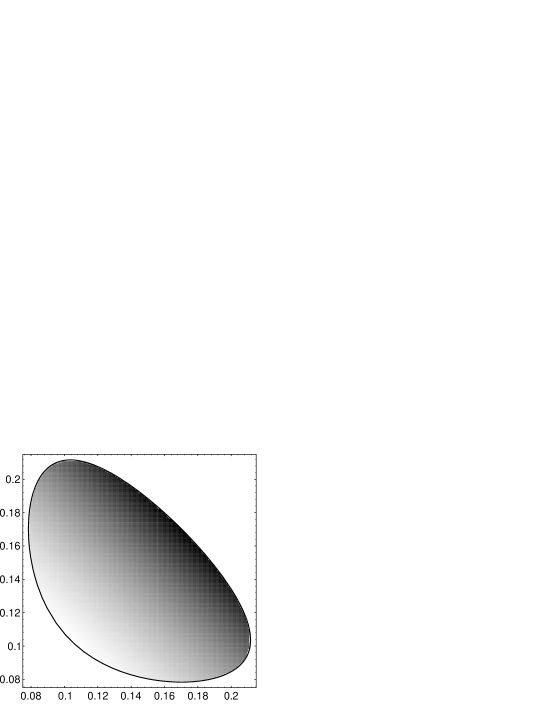
$\displaystyle\displaystyle s_{2}\,[\mbox{GeV}^{2}]$        

The numerical results for the integrated branching ratio with $\displaystyle Q^{2}\leq Q^{2}_{max}$ for CHPT at $\displaystyle O(p^{2})$ and $\displaystyle O(p^{4})$ are given in Tab. 2. The series expansion of CHPT does not seem to behave very well. Even for $\displaystyle Q_{max}=500\,\mbox{MeV}$, the integrated one loop contribution is already around 45 % of the tree level result. This means that to have a CHPT prediction with a reasonably small theoretical uncertainty for such a quantity one should stop at $\displaystyle Q_{max}$ well below $\displaystyle 500\,\mbox{MeV}$, and this would be very difficult to test experimentally, because of the strong phase space suppression of this region. On the other hand we observe that there is a fair agreement with the VMD model numbers up to $\displaystyle Q_{max}=600\,\mbox{MeV}$, which is better than what happens in the two pion case. This can be understood in terms of the fact that in the two pion case, the $\displaystyle\rho(770)$ resonance is very close, whereas in the three pion case, the nearest three pion resonance, the $\displaystyle a_{1}(1260)$, is much further away. Whether the VMD model is a good representation of the experimental data even at such a low energy though, has still to be verified.

Beyond the integrated decay rates, this decay mode has a very rich structure, which in principle could be investigated in detail experimentally. In fact in [27] it has been shown that it is possible to extract all three form factors from a measurement of all angular distributions. One could then compare the measured form factors to the analytic formulae of CHPT. This extraction is however very difficult in practice, and moreover the phase space suppresses considerably the region where the comparison makes sense. For these reasons we find more useful to show directly the curves for the integrated structure functions $\displaystyle w_{X}$ in Figs. 2–7. We have chosen six out of the nine structure functions which are present, mainly because the missing three are too difficult to be measured and not particularly interesting. Note that, in accordance with our definitions in Eqs. (31,A.1), the Cabibbo angle $\displaystyle\cos^{2}\theta_{C}$ is factored out from hadronic matrix element, and so the structure functions $\displaystyle w_{X}$ do not include this factor.

In Fig. 2 we plot $\displaystyle w_{A}(Q^{2})$ for the $\displaystyle 2\pi^{-}\pi^{+}$ final state. It turns out that $\displaystyle w_{A}(Q^{2})$ and $\displaystyle w_{C}(Q^{2})$ for both charge states, $\displaystyle 2\pi^{-}\pi^{+}$ and $\displaystyle 2\pi^{0}\pi^{-}$ are all very similar, so the four plots can not be distinguished from each other. The equality of the structure functions for the two charge modes suggests that $\displaystyle w_{A}$ and $\displaystyle w_{C}$ are dominated by the [210] partition. We have explicitly verified that this is the case: for example at $\displaystyle Q^{2}=15M_{\pi}^{2}$ the $\displaystyle[210]$ partition contributes $\displaystyle 6.73\times 10^{-2}\mbox{GeV}^{-4}$ to $\displaystyle w_{A}$ for both modes, whereas the $\displaystyle[300]$ partition contributes $\displaystyle 2.21\times 10^{-4}\mbox{GeV}^{-4}$ for the $\displaystyle 2\pi^{-}\pi^{+}$ and, according to Eq. (28), one quarter of this for the $\displaystyle 2\pi^{0}\pi^{-}$ mode. The interference of the two partitions is completely negligible.

The reason why $\displaystyle w_{A}\sim w_{C}$ at low energy is that

$$\displaystyle W_{C} \displaystyle= \displaystyle W_{A}-2x_{3}^{2}|F_{1}-F_{2}|^{2}$$ (55)

$$\displaystyle= \displaystyle W_{A}-8x_{3}^{2}|H|^{2}\;.$$

Since $\displaystyle H$ is zero at tree level, the difference vanishes at leading order. Moreover this difference starts as the square of a quantity of $\displaystyle O(p^{2})$. Using the language of the sixties we can say that the vanishing of this difference near threshold is a Low Energy Theorem (LET), and that it receives corrections only at next–to–next–to–leading order. We also notice that $\displaystyle H$ is a function antisymmetric under exchange of $\displaystyle s_{1}$ and $\displaystyle s_{2}$, so that its modulus squared has a zero along the line $\displaystyle s_{1}=s_{2}$. At low energy, where the distance between this line and the boundaries of integration is not large (in units of $\displaystyle M_{\pi}^{2}$), the presence of the zero produces an additional suppression of the integral. The similarity of these two functions near threshold was already found in Ref. [26, 27] in the framework of a VMD model. Here however, we can give a detailed algebraic account of why this happens. For all these arguments we believe that this fact should be verified experimentally even at energies well above those where one would trust a one loop CHPT calculation.

In Fig. 3 and 4 we plot $\displaystyle w_{D}(Q^{2})$ and $\displaystyle w_{E}(Q^{2})$. These are much smaller than $\displaystyle w_{A}$ near threshold, and certainly more difficult to be measured. However they seem rather interesting from a theoretical point of view. First of all for both of them the $\displaystyle O(p^{2})$ contribution vanishes. Secondly, the $\displaystyle O(p^{4})$ predictions from CHPT differ strongly for the two charge modes. According to the discussion in Sec. 3.3.2, this fact suggests that near threshold these two structure functions are strongly influenced by the partition $\displaystyle[300]$. Using the decomposition of the form factors given in Eq. (3.3.2), we have verified that this is exactly what happens. As can be seen in Tab. 3 the change of sign in the interference contribution is responsible for the change of sign of the whole integrated structure functions in the two different charge modes.

		$\displaystyle[300]$	$\displaystyle[210]$	interf.	total
	$\displaystyle(2\pi^{-}\pi^{+})$	$\displaystyle 8.63\times 10^{-2}$	$\displaystyle 1.02$	$\displaystyle-1.56$	$\displaystyle-0.450$
$\displaystyle 10^{3}w_{D}$
	$\displaystyle(2\pi^{0}\pi^{-})$	$\displaystyle 2.16\times 10^{-2}$	$\displaystyle 1.02$	$\displaystyle 0.779$	$\displaystyle 1.82$
	$\displaystyle(2\pi^{-}\pi^{+})$	$\displaystyle 4.62\times 10^{-4}$	$\displaystyle 0.206$	$\displaystyle 2.08$	$\displaystyle 2.29$
$\displaystyle 10^{3}w_{E}$
	$\displaystyle(2\pi^{0}\pi^{-})$	$\displaystyle 1.16\times 10^{-4}$	$\displaystyle 0.206$	$\displaystyle-1.04$	$\displaystyle-0.837$

Table 3: Splitting of the integrated structure functions $\displaystyle w_{E}$ and $\displaystyle w_{D}$ into the contributions of the partitions $\displaystyle[300],\;[210]$ and their interference, at $\displaystyle Q^{2}=15M_{\pi}^{2}$.

As far as we know up to now there are no data for these structure functions so close to threshold: so this is a real prediction of CHPT. Moreover this change of sign is absent in all the models of which we are aware which have been used to describe this decay channel. It is then important to ask how reliable this prediction is and up to what energy it can be trusted. These questions are especially difficult to answer here because we have only a leading order calculation (since the $\displaystyle O(p^{2})$ contribution vanishes). The only thing we can do is to check how sensitive the prediction is to the values we use for the low energy constants. We concentrate here on the $\displaystyle[300]$ state, since it is the one responsible for the new effect:

$$\displaystyle\frac{F_{\pi}^{3}}{i\sqrt{2}}F_{1}^{[300]} \displaystyle= \displaystyle\frac{1}{72\pi^{2}}\left[\bar{l}_{1}+\bar{l}_{2}-3\right]\left(\frac{Q^{2}}{3}-s_{1}+M_{\pi}^{2}\right)$$ (56)

$$\displaystyle+ \displaystyle\frac{4}{9}\bar{J}(s_{1})(M_{\pi}^{2}-s_{1})-\frac{2}{9}\bar{J}(s_{2})(s_{2}-M_{\pi}^{2})-\frac{2}{9}\bar{J}(s_{2})(s_{2}-M_{\pi}^{2})\;.$$

First of all we notice that this partition has no contribution from tree level. This is not the case for the $\displaystyle[210]$ partition, which starts as:

$$\frac{F_{\pi}}{i\sqrt{2}}F_{1}^{[210]}=\frac{2}{3}+O(p^{2})\;.$$ (57)

This explains why the interference contribution is much bigger than the one from the $\displaystyle[300]$ partition alone. Then we may easily see from the definition of these two structure functions given in App. A.3 that the $\displaystyle w_{D}$ is mainly sensitive to the real part of $\displaystyle F_{1}^{[300]}$, whilst $\displaystyle w_{E}$ to the imaginary part. This means that only the numbers for $\displaystyle w_{D}$ may depend on the combination of low energy constants which occurs in $\displaystyle F_{1}^{[300]}$. The value used for the combination $\displaystyle\bar{l}_{1}+\bar{l}_{2}-3$ in the numerical calculations is $\displaystyle 1.4$, resulting from the central values given in Tab. 1. The uncertainty on this number can be estimated from the same Tab. 1 to be $\displaystyle\pm 1.1$. So the possibility that the real value of this combination be twice as much, or very close to zero cannot be excluded. We have checked that by changing the value of $\displaystyle\bar{l}_{1}+\bar{l}_{2}-3$ by $\displaystyle\pm 1.4$ changes $\displaystyle w_{D}$ in the $\displaystyle 2\pi^{-}\pi^{+}$ mode by $\displaystyle\pm 4.4\times 10^{-4}$, at $\displaystyle Q^{2}=15M_{\pi}^{2}$. As expected $\displaystyle w_{E}$ remains practically unchanged. Even in the worst case for $\displaystyle w_{D}$, however, there remains a sizable difference between the two charge modes. The effect of higher orders in the chiral expansion and the related questions of how far in energy one can trust this prediction will remain unanswered until one calculates the form factors at two loops, which is beyond the scope of our analysis. We may just argue that since there are no low-lying resonances contributing to this particular three pion state, one of the possible sources of large higher order corrections is excluded.

All in all we can say that CHPT predicts a sign difference in the two structure functions $\displaystyle w_{D}$ and $\displaystyle w_{E}$ for the two charge modes near threshold. This prediction will have interesting consequences in the next subsection, where we compare with VMD models and available data.

In Fig. 5 we plot $\displaystyle w_{SA}(Q^{2})$ for the $\displaystyle 2\pi^{-}\pi^{+}$ state. The corresponding curves for the $\displaystyle 2\pi^{0}\pi^{-}$ state in Fig. 6 have a very similar shape but a different overall normalization. In fact, the ratio $\displaystyle w_{SA}^{2\pi^{-}\pi^{+}}/w_{SA}^{2\pi^{0}\pi^{-}}$ is close to 4, which according to Sec. 3.3.2 implies that the scalar form factor at low energies is dominated by the [300] state.

We find that the structure function $\displaystyle w_{SA}$ is very small compared to $\displaystyle w_{A}$, so the spin-0 contribution to the integrated rate is negligible. The only chance to measure the spin-0 part is via its interference with the spin-1 part in the structure function $\displaystyle w_{SB}(Q^{2})$, which is plotted in Fig. 7.

In Fig. 8 we consider the Dalitz plot distribution $\displaystyle d\Gamma/(dQ^{2}\,ds_{1}\,ds_{2})$ in $\displaystyle s_{1}$, $\displaystyle s_{2}$ for fixed $\displaystyle Q^{2}=0.36\,\mbox{GeV}^{2}$. We display the $\displaystyle O(p^{4})$ prediction for the $\displaystyle 2\pi^{-}\pi^{+}$ mode. At $\displaystyle O(p^{2})$, the Dalitz plot density depends only on $\displaystyle s_{1}+s_{2}$. As seen from the figure, this feature seems to persist at $\displaystyle O(p^{4})$. Let us analyze this issue quantitatively. To describe the Dalitz plot, we define $\displaystyle s_{+}$ and $\displaystyle s_{-}$ by

$$s_{+}:=s_{1}+s_{2},\qquad s_{-}:=s_{1}-s_{2}$$ (58)

and then replace $\displaystyle s_{+},s_{-}$ by dimensionless variables $\displaystyle x,y$ with $\displaystyle 0\leq x\leq 1$ and $\displaystyle-1\leq y\leq 1$ via

$$\displaystyle s_{+} \displaystyle= \displaystyle(s_{+}^{\rm max}-s_{+}^{\rm min})x+s_{+}^{\rm min}$$

$$\displaystyle s_{-} \displaystyle= \displaystyle s_{-}^{\rm max}y$$ (59)

where

$$\displaystyle s_{+}^{\rm min} \displaystyle= \displaystyle 2m_{\pi}(m_{\pi}+\sqrt{{Q^{2}}})$$

$$\displaystyle s_{+}^{\rm max} \displaystyle= \displaystyle{Q^{2}}-m_{\pi}^{2}$$

$$\displaystyle s_{-}^{\rm max} \displaystyle= \displaystyle\sqrt{\frac{[s_{+}(s_{+}-4m_{\pi}^{2})-4m_{\pi}^{2}({Q^{2}}-m_{\pi}^{2})][{Q^{2}}-s_{+}-m_{\pi}^{2}]}{{Q^{2}}+3m_{\pi}^{2}-s_{+}}}$$ (60)

We perform a least-square fit to the Dalitz plot density as predicted by CHPT, using a fit function

$$\rho_{Q^{2}}(x,y):=\frac{d\Gamma}{dQ^{2}\,ds_{1}\,ds_{2}}=a(x+b+cx^{2}+dx^{3}+ex^{4}+fx(x-1)y^{2})$$ (61)

Note that this is a reasonable ansatz for the $\displaystyle y$ dependence. Firstly, we must have $\displaystyle\rho_{Q^{2}}(x,y)=\rho_{Q^{2}}(x,-y)$ because of Bose symmetry. Secondly, at $\displaystyle x\to 0$ and at $\displaystyle x\to 1$, $\displaystyle s_{-}^{max}\to 0$, so the dependence on $\displaystyle y^{2}$ must go to zero at $\displaystyle x=0,1$.

We choose to discuss the CHPT predictions for $\displaystyle Q^{2}=0.36\,\mbox{GeV}^{2}$. At this value of $\displaystyle Q^{2}$, the result from the fit is

$$\displaystyle a \displaystyle= \displaystyle(3.0360\pm 0.0095)\times 10^{-14}\,\mbox{GeV}^{-5}$$

$$\displaystyle b \displaystyle= \displaystyle(5.251\pm 0.039)\times 10^{-3}$$

$$\displaystyle c \displaystyle= \displaystyle(0.786\pm 0.023)$$

$$\displaystyle d \displaystyle= \displaystyle(0.190\pm 0.053)$$

$$\displaystyle e \displaystyle= \displaystyle(0.189\pm 0.036)$$

$$\displaystyle f \displaystyle= \displaystyle(0.0645\pm 0.0026)$$ (62)

This fit never deviates from the CHPT prediction by more than $\displaystyle 2\%$, with an average deviation of less than $\displaystyle 1\%$. It is seen that the $\displaystyle y^{2}$ dependence is very small. In fact, taking into account that the coefficient $\displaystyle x(x-1)$, which multiplies $\displaystyle y^{2}$, is less or equal to $\displaystyle 1/4$, we find that the leading $\displaystyle y$ dependence does not exceed $\displaystyle 2\%$. We have checked that, as one would expect, the $\displaystyle y^{2}$ dependence is even smaller for smaller $\displaystyle Q^{2}$.

This Dalitz plot distribution, as predicted by CHPT for $\displaystyle Q^{2}\leq 0.36\,\mbox{GeV}^{2}$, differs strongly from the behavior at high $\displaystyle Q^{2}$ in the resonance regime, where the $\displaystyle\rho$ resonances lead to pronounced structures in $\displaystyle s_{1}$ and $\displaystyle s_{2}$ (resonance bands for fixed $\displaystyle s_{1}$ or $\displaystyle s_{2}$) [37].

5.3 Comparison with Vector Meson Dominance Models

In this subsection we will compare with the low energy behavior of the phenomenological models in [5, 7, 8]. The simplest VMD model which one can build for this channel (see Ref. [5]) is based on the decay chain $\displaystyle\tau\to a_{1}\nu_{\tau}$, $\displaystyle a_{1}\to\rho\pi$, $\displaystyle\rho\to 2\pi$ and a transverse $\displaystyle a_{1}$ propagator. In this case the amplitude contains only a spin 1 part ($\displaystyle F_{S}=0$), and the three pions are only in a $\displaystyle[210]$ partition state ($\displaystyle F_{1}^{[300]}=0$). The comparison to the data [38, 39] shows that the model works well, which means that the assumptions made are reasonable.

However it is clear that these assumptions need not be strictly true in the physical reality, so the authors of Refs. [7, 8] have tried to include in the VMD model a nonzero scalar form factor. Two possible sources for a non-vanishing $\displaystyle F_{S}$, are a pseudoscalar three-pion resonance, the $\displaystyle\pi^{\prime}$, or the non-transverse component of the off-shell $\displaystyle a_{1}$ propagator. A model for the $\displaystyle\pi^{\prime}$ contribution is given in [7]. The numerical impact of the $\displaystyle\pi^{\prime}$ depends on a parameter $\displaystyle f_{\pi^{\prime}}$. In [7] and in its implementation in TAUOLA [33] a particularly large value from [2] has been chosen, which is probably several orders of magnitude too large [40]. However, we find that even with this high value of $\displaystyle f_{\pi^{\prime}}$, the contribution from the $\displaystyle\pi^{\prime}$ to the scalar form factor at low energies is much smaller than the predictions from CHPT. This indicates that — at least at small energies — there are additional contributions to $\displaystyle F_{S}$. The off-shell contribution of the $\displaystyle a_{1}$ to $\displaystyle F_{S}$ is discussed in [8]. A specific model is constructed by matching to the $\displaystyle O(p^{2})$ prediction of CHPT (including the $\displaystyle M_{\pi}^{2}\neq 0$ effects), and we will compare this model with the CHPT predictions.

On the other hand, the presence of a $\displaystyle[300]$ component in the spin 1 form factor has never been proposed in any of these models. With our calculation we can make a detailed analytical comparison between VMD models and the CHPT amplitude at low energy. The main conclusion is that even in the region close to threshold the VMD model works rather well.

First we consider the structure functions which only involve the $\displaystyle F_{1}$. After a proper normalization of the form factors in the VMD model, which takes into account the CHPT expressions at $\displaystyle O(p^{2})$, the agreement for the spin one spectral function at low energy looks very good. This can be seen in Fig. 2, where we plot $\displaystyle w_{A}$, i.e. the main contribution to the total decay rate. Moreover the $\displaystyle[300]$ component of $\displaystyle F_{1}$ starts only at one loop, which means that in the chiral expansion this is algebraically suppressed with respect to the $\displaystyle[210]$ part.

However, the - numerically rather small - structure functions $\displaystyle w_{D}$ and $\displaystyle w_{E}$ are sensitive to the $\displaystyle[300]$ part via interference with the $\displaystyle[210]$ part, as we have seen in the previous subsection. Comparing the VMD model with the CHPT prediction for these structure functions in Figs. 3 and 4, we find good agreement for $\displaystyle 2\pi^{0}\pi^{-}$, but flat disagreement for $\displaystyle 2\pi^{-}\pi^{+}$. However, at larger $\displaystyle Q^{2}$, experimental data for $\displaystyle w_{D}$ and $\displaystyle w_{E}$ in $\displaystyle 2\pi^{-}\pi^{+}$ are available, which agree with the VMD prediction [38, 39]. Note that the left-right asymmetry $\displaystyle A_{LR}(Q^{2})$ measured by ARGUS [38] is proportional to $\displaystyle w_{E}(Q^{2})/w_{A}(Q^{2})$ [26], and confirms the VMD prediction in sign and magnitude down to $\displaystyle Q^{2}=0.8\,\mbox{GeV}^{2}.$ We conclude that, unless the higher orders in the chiral expansion completely change the CHPT result, somewhere between threshold and $\displaystyle Q^{2}=0.8\mbox{GeV}^{2}$ there must be a zero for both structure functions in the $\displaystyle 2\pi^{-}\pi^{+}$ mode. It would be extremely interesting to verify this zero experimentally, or, as a minimal option, to verify the existence of a difference between the two charge modes.

Next we consider the scalar form factor: Although $\displaystyle F_{S}$ is nonzero already at tree level, it is kinematically suppressed:

$$\displaystyle F_{1} \displaystyle= \displaystyle\frac{i\sqrt{2}}{F_{\pi}}\left(\frac{2}{3}+O(p^{2})\right)\;,$$

$$\displaystyle F_{S} \displaystyle= \displaystyle\frac{i\sqrt{2}}{F_{\pi}}\left(\frac{M_{\pi}^{2}}{Q^{2}}\frac{s_{3}-M_{\pi}^{2}}{M_{\pi}^{2}-Q^{2}}+O(p^{2})\right)\;.$$ (63)

Though $\displaystyle Q^{2},s_{3}$ and $\displaystyle M_{\pi}^{2}$ are all counted as quantities of order $\displaystyle p^{2}$, so that the ratios $\displaystyle M_{\pi}^{2}/Q^{2}$ and $\displaystyle s_{3}/Q^{2}$ are algebraically of order one, it is clear that numerically they are smaller than one. For example at threshold $\displaystyle F_{S}=i\sqrt{2}/F_{\pi}(-1/24)=-1/16\times F_{1}$.

In Figs. 5,6 and 7, where we plot the two structure functions $\displaystyle w_{SA}$ and $\displaystyle w_{SB}$, one can see the comparison of the VMD model in [8] to CHPT at $\displaystyle O(p^{4})$. We find that the VMD model, which by construction reproduces the $\displaystyle O(p^{2})$ prediction, does not reproduce well the $\displaystyle O(p^{4})$ prediction from CHPT. The reason for this discrepancy (which is larger for $\displaystyle w_{SA}$, since it contains the scalar form factor squared) lies in the fact that in the model in [8], the $\displaystyle[300]$ part of $\displaystyle F_{S}$ is added as a constant, without a resonance factor enhancement.

Summarizing our comparison of CHPT and VMD predictions at low energies, we have found that VMD gives a good description of the dominant spin-1, $\displaystyle[210]$ contribution. However, CHPT shows that both $\displaystyle F_{S}$ and $\displaystyle F_{1}^{[300]}$, though small, are not exactly zero. This fact, which is a prediction of CHPT, has still to be verified experimentally. Our analysis shows that the best place to look for these parts of the amplitude, is where they can interfere with the “big” components: the presence of $\displaystyle F_{S}$ should be detected by measuring a nonzero $\displaystyle w_{SB}$, whereas the presence of $\displaystyle F_{1}^{[300]}$ should be discovered by measuring a sizable difference (possibly a sign difference) between the two charge modes for $\displaystyle w_{D}$ and $\displaystyle w_{E}$.

6 Summary and Conclusions

Chiral perturbation theory (CHPT) provides model-independent predictions for hadronic matrix elements in the low energy region below $\displaystyle 500\cdots 600\,\mbox{MeV}$. It does not contain additional assumptions beyond the fact that the strong interactions are described by the QCD Lagrangian and that QCD possesses an approximate chiral symmetry which is spontaneously broken. We have evaluated tau decays into two pions (and tau-neutrino) to two loops and decays into three pions to the one loop level. The branching ratio into the phase space region with small enough invariant hadronic mass for CHPT to be applicable was found to be about $\displaystyle 4\times 10^{-3}$ for the two pion mode and about $\displaystyle 10^{-5}$ for the three pion mode. And so the predictions of CHPT for $\displaystyle\tau\to 2\pi\nu_{\tau}$ are testable at present machines (LEP and CESR), while in the case of $\displaystyle\tau\to 3\pi\nu_{\tau}$, future facilities with very high $\displaystyle\tau$ production rates seem to be required (b factories, $\displaystyle\tau$-charm factory).

In the case of the decay $\displaystyle\tau\to 2\pi\nu_{\tau}$, the predictions for the invariant mass distributions can be tested at present experiments, and the spectrum can be used to extract the pion charge radius $\displaystyle\langle r^{2}\rangle_{V}^{\pi}$.

As for the decay $\displaystyle\tau\to 3\pi\nu_{\tau}$, a detailed comparison to the CHPT predictions for the form factors near threshold requires very high statistics, mainly because of the phase space suppression. For this reason we have tried to identify a few spots where the consequences of the approximate chiral symmetry of QCD can be tested experimentally with a reasonable statistics. These are:

1. the very close similarity of $\displaystyle w_{A}$ and $\displaystyle w_{C}$ near threshold, which seems to extend well beyond the very low energy region;

2. a zero and change of sign in $\displaystyle w_{D}$ and $\displaystyle w_{E}$ between threshold and $\displaystyle Q^{2}\sim 0.8\mbox{GeV}^{2}$ in the channel $\displaystyle 2\pi^{-}\pi^{+}$, or at least a difference between the two charge modes near threshold. This would be the first evidence for the presence of the $\displaystyle[300]$ partition state in this decay channel;

3. the presence of a scalar form factor as predicted by CHPT, to be detected by measuring $\displaystyle w_{SB}$.

Comparing our results to predictions from vector meson dominance models, we find overall a reasonable agreement in the low energy region. The structure function $\displaystyle w_{A}$, which dominates the decay rate, is described well by VMD models. We have found, however, some interesting discrepancies in certain (numerically rather small) structure functions. These discrepancies are related to the [300] partition state and to the scalar form factor, which both are missing or underestimated in vector meson dominance models.

Appendix A Appendix

A.1 General conventions

Consider the decay of a tau into $\displaystyle n$ pions,

$$\tau(p,s)\to\nu_{\tau}(q,s^{\prime})\pi_{1}(p_{1})\pi_{2}(p_{2})\cdots\pi_{n}(p_{n})$$ (64)

Here $\displaystyle s$ and $\displaystyle s^{\prime}$ denote the polarization four-vectors of the tau and the neutrino, respectively. We define the total hadronic momentum $\displaystyle Q$ by

$$Q=p_{1}+p_{2}+\cdots+p_{n}$$ (65)

and in the case of three pions, we will use Dalitz plot invariants $\displaystyle s_{1}$, $\displaystyle s_{2}$ and $\displaystyle s_{3}$ defined by

$$s_{1}=(p_{2}+p_{3})^{2}$$ (66)

and cyclic permutations.

The differential decay rate $\displaystyle d\Gamma_{n}$ is given by

$$d\Gamma_{n}=\frac{1}{2M_{\tau}}|{\cal M}|^{2}d\Phi_{n}$$ (67)

where the phase space element $\displaystyle d\Phi_{n}$ is

$$d\Phi_{n}=(2\pi)^{4}\delta(Q+q-p)\frac{d^{3}q}{(2\pi)^{3}2E_{\nu}}\prod_{k=1}^{n}\frac{d^{3}p_{k}}{(2\pi)^{3}2E_{k}}$$ (68)

and

$$\displaystyle{\cal M} \displaystyle= \displaystyle\frac{G_{F}}{\sqrt{2}}\cos\theta_{C}L_{\mu}H^{\mu}$$

$$\displaystyle L_{\mu} \displaystyle= \displaystyle\overline{u}_{\nu}(q,s^{\prime})\gamma_{\mu}\gamma_{-}u_{\tau}(p,s)$$

$$\displaystyle H_{\mu} \displaystyle= \displaystyle\langle\pi_{1}(p_{1})\pi_{2}(p_{2})\dots\pi_{n}(p_{n})|V_{\mu}(0)-A_{\mu}(0)|0\rangle$$ (69)

A.2 Decomposition of the form factors in terms of partition states

As we discussed in Sect. 3.3.2, we have three possible partition states, two belonging to the class $\displaystyle[210]$ (which we will indicate as $\displaystyle[210]_{a}$ and $\displaystyle[210]_{b}$) and one belonging to the class $\displaystyle[300]$. The matrix elements of these states are easily constructed by performing the appropriate symmetrizations and antisymmetrizations with respect to momenta exchanges, as described in Sect. 3.3.2. The result can be expressed in terms of the three form factors $\displaystyle F,\;G$ and $\displaystyle H$, and reads as follows:

$$\displaystyle F^{[210]_{a}} \displaystyle= \displaystyle\frac{2}{3}\left[F_{12}-G_{23}+H_{23}\right]$$

$$\displaystyle G^{[210]_{a}} \displaystyle= \displaystyle\frac{2}{3}\left[G_{12}-\frac{1}{2}\left(F_{23}+G_{23}+H_{23}\right)\right]$$

$$\displaystyle H^{[210]_{a}} \displaystyle= \displaystyle\frac{2}{3}\left[H_{12}-\frac{1}{2}\left(F_{23}-G_{23}-H_{23}\right)\right]\;,$$ (70)

$$\displaystyle F^{[210]_{b}} \displaystyle= \displaystyle\frac{1}{3}\left[-G_{13}+G_{23}+H_{13}-H_{23}\right]$$

$$\displaystyle G^{[210]_{b}} \displaystyle= \displaystyle\frac{1}{6}\left[-F_{13}+F_{23}-G_{13}+G_{23}-H_{13}+H_{23}\right]$$

$$\displaystyle H^{[210]_{b}} \displaystyle= \displaystyle\frac{1}{6}\left[F_{13}+F_{23}-G_{13}-G_{23}-H_{13}-H_{23}\right]\;,$$ (71)

$$\displaystyle F^{[300]} \displaystyle= \displaystyle\frac{1}{3}\left[F_{12}+G_{13}+G_{23}-H_{13}-H_{23}\right]$$

$$\displaystyle G^{[300]} \displaystyle= \displaystyle\frac{1}{3}\left[G_{12}+\frac{1}{2}\left(F_{13}+F_{23}+G_{13}+G_{23}+H_{13}+H_{23}\right)\right]$$

$$\displaystyle H^{[300]} \displaystyle= \displaystyle\frac{1}{3}\left[H_{12}+\frac{1}{2}\left(-F_{13}+F_{23}+G_{13}-G_{23}+H_{13}-H_{23}\right)\right]\;,$$ (72)

where $\displaystyle X_{ij}=X(s_{i},s_{j},s_{k})$, $\displaystyle X=F,G,H$ and $\displaystyle k\neq i\neq j$. To reconstruct the form factors in the two charge modes one has to use the relations:

$$\displaystyle X_{12} \displaystyle= \displaystyle X^{[300]}+X^{[210]_{a}}+X^{[210]_{b}}$$

$$\displaystyle X^{(+)}_{12} \displaystyle= \displaystyle 2X^{[300]}-X^{[210]_{a}}-X^{[210]_{b}}\;.$$ (73)

A.3 Structure functions for the three pion final state

In this section we will briefly review the formalism of structure functions for the decay of the tau into three pions, and display formulae relevant for the present paper. For more details, the reader is referred to [26, 27].

The decays are most easily analyzed in the hadronic rest frame

$$\vec{0}=\vec{Q}=\vec{p_{1}}+\vec{p_{2}}+\vec{p_{3}}$$ (74)

The orientation of the hadronic system is characterized by three Euler angles $\displaystyle\alpha$, $\displaystyle\beta$, $\displaystyle\gamma$, as introduced in [26, 27]. They can be defined by ($\displaystyle 0\leq\alpha,\gamma<2\pi$; $\displaystyle 0\leq\beta<\pi$)

$$\displaystyle\cos\alpha=\frac{(\vec{n}_{L}\times\vec{n}_{\tau})\cdot(\vec{n}_{L}\times\vec{n}_{\perp})}{|\vec{n}_{L}\times\vec{n}_{\tau}||\vec{n}_{L}\times\vec{n}_{\perp}|} \displaystyle\sin\alpha=-\frac{\vec{n}_{\tau}\cdot(\vec{n}_{L}\times\vec{n}_{\perp})}{|\vec{n}_{L}\times\vec{n}_{\tau}||\vec{n}_{L}\times\vec{n}_{\perp}|}$$

$$\displaystyle\cos\gamma=-\frac{\vec{n}_{L}\cdot\vec{n}_{3}}{\vec{n}_{L}\times\vec{n}_{\perp}} \displaystyle\sin\gamma=\frac{(\vec{n}_{L}\times\vec{n}_{\perp})\cdot\vec{n}_{3}}{\vec{n}_{L}\times\vec{n}_{\perp}}$$

$$\displaystyle\cos\beta=\vec{n}_{L}\cdot\vec{n}_{\perp}$$ (75)

where $\displaystyle\vec{n}_{L}$ is the direction of the laboratory in the hadronic rest frame, $\displaystyle\vec{n}_{\perp}=(\vec{p}_{1}\times\vec{p}_{2})/(|\vec{p}_{1}\times\vec{p}_{2}|)$ is the normal to the pion plane (here we assign the momenta according to $\displaystyle|\vec{p_{2}}|>|\vec{p_{1}}|$), $\displaystyle\vec{n}_{\tau}$ is the direction of flight of the $\displaystyle\tau$ in the hadronic rest frame and $\displaystyle\vec{n}_{3}=\vec{p}_{3}/|\vec{p}_{3}|$.

From these definition it is obvious that $\displaystyle\beta$ and $\displaystyle\gamma$ are observable even if the tau rest frame cannot be reconstructed, whereas $\displaystyle\alpha$ does require this knowledge. $\displaystyle\alpha$ could be measured at a tau-charm factory where the tau pairs are produced almost at rest and therefore the tau rest frame is known, or if the tau direction can be measured with the help of vertex detectors [41].

The Euler angles also serve to parameterize the phase space

$$dPS^{(4)}=\frac{1}{(2\pi)^{5}}\frac{1}{64}\frac{M_{\tau}^{2}-Q^{2}}{M_{\tau}^{2}}\frac{dQ^{2}}{Q^{2}}ds_{1}\,ds_{2}\frac{d\alpha}{2\pi}\frac{d\gamma}{2\pi}\frac{d\cos\beta}{2}\frac{d\cos\theta}{2}$$ (76)

where $\displaystyle\theta$ is the angle between the direction of flight of the $\displaystyle\tau$ in the laboratory frame and the direction of the pions as seen in the $\displaystyle\tau$ rest frame, and $\displaystyle\cos\theta$ can be calculated from the energy $\displaystyle E_{h}$ of the pion system with respect to to the laboratory frame and beam energy $\displaystyle E_{beam}$

$$\cos\theta=\frac{2E_{h}/E_{b}M_{\tau}^{2}-M_{\tau}^{2}-Q^{2}}{(M_{\tau}^{2}-Q^{2})\sqrt{1-M_{\tau}^{2}/E_{beam}^{2}}}$$ (77)

The contraction of the leptonic and hadronic tensors can be expanded in a sum

$$L_{\mu\nu}H^{\mu\nu}=\sum_{X}L_{X}W_{X}$$ (78)

In general, $\displaystyle H^{\mu\nu}$ can be characterized by 16 independent real functions. In our case of a three pion final states, there are restrictions due to $\displaystyle G$ parity and Bose symmetry, which leave 9 independent functions. In a convenient basis they are given by [27]

$$\displaystyle\hskip 8.53581ptW_{A} \displaystyle= \displaystyle\hskip 8.53581pt(x_{1}^{2}+x_{3}^{2})\,|F_{1}|^{2}+(x_{2}^{2}+x_{3}^{2})\,|F_{2}|^{2}+2(x_{1}x_{2}-x_{3}^{2})\,\mbox{Re}\left(F_{1}F^{\ast}_{2}\right)$$

$$\displaystyle W_{B} \displaystyle= \displaystyle\hskip 8.53581ptx_{4}^{2}|F_{3}|^{2}$$

$$\displaystyle W_{C} \displaystyle= \displaystyle\hskip 8.53581pt(x_{1}^{2}-x_{3}^{2})\,|F_{1}|^{2}+(x_{2}^{2}-x_{3}^{2})\,|F_{2}|^{2}+2(x_{1}x_{2}+x_{3}^{2})\,\mbox{Re}\left(F_{1}F^{\ast}_{2}\right)$$

$$\displaystyle W_{D} \displaystyle= \displaystyle\hskip 8.53581pt2\left[x_{1}x_{3}\,|F_{1}|^{2}-x_{2}x_{3}\,|F_{2}|^{2}+x_{3}(x_{2}-x_{1})\,\mbox{Re}\left(F_{1}F^{\ast}_{2}\right)\right]$$

$$\displaystyle W_{E} \displaystyle= \displaystyle-2x_{3}(x_{1}+x_{2})\,\mbox{Im}\left(F_{1}F^{\ast}_{2}\right)$$

$$\displaystyle W_{F} \displaystyle= \displaystyle\hskip 8.53581pt2x_{4}\left[x_{1}\,\mbox{Im}\left(F_{1}F^{\ast}_{3}\right)+x_{2}\,\mbox{Im}\left(F_{2}F^{\ast}_{3}\right)\right]$$

$$\displaystyle W_{G} \displaystyle= \displaystyle-2x_{4}\left[x_{1}\,\mbox{Re}\left(F_{1}F^{\ast}_{3}\right)+x_{2}\,\mbox{Re}\left(F_{2}F^{\ast}_{3}\right)\right]]$$

$$\displaystyle W_{H} \displaystyle= \displaystyle\hskip 8.53581pt2x_{3}x_{4}\left[\,\mbox{Im}\left(F_{1}F^{\ast}_{3}\right)-\,\mbox{Im}\left(F_{2}F^{\ast}_{3}\right)\right]$$ (79)

$$\displaystyle W_{I} \displaystyle= \displaystyle-2x_{3}x_{4}\left[\,\mbox{Re}\left(F_{1}F^{\ast}_{3}\right)-\,\mbox{Re}\left(F_{2}F^{\ast}_{3}\right)\right]$$

$$\displaystyle W_{SA} \displaystyle= \displaystyle\hskip 8.53581ptQ^{2}\,|F_{4}|^{2}$$

$$\displaystyle W_{SB} \displaystyle= \displaystyle\hskip 8.53581pt2\sqrt{Q^{2}}\left[x_{1}\,\mbox{Re}\left(F_{1}F^{\ast}_{4}\right)+x_{2}\,\mbox{Re}\left(F_{2}F^{\ast}_{4}\right)\right]$$

$$\displaystyle W_{SC} \displaystyle= \displaystyle-2\sqrt{Q^{2}}\left[x_{1}\,\mbox{Im}\left(F_{1}F^{\ast}_{4}\right)+x_{2}\,\mbox{Im}\left(F_{2}F^{\ast}_{4}\right)\right]$$

$$\displaystyle W_{SD} \displaystyle= \displaystyle\hskip 8.53581pt2\sqrt{Q^{2}}x_{3}\left[\,\mbox{Re}\left(F_{1}F^{\ast}_{4}\right)-\,\mbox{Re}\left(F_{2}F^{\ast}_{4}\right)\right]$$

$$\displaystyle W_{SE} \displaystyle= \displaystyle-2\sqrt{Q^{2}}x_{3}\left[\,\mbox{Im}\left(F_{1}F^{\ast}_{4}\right)-\,\mbox{Im}\left(F_{2}F^{\ast}_{4}\right)\right]$$

$$\displaystyle W_{SF} \displaystyle= \displaystyle-2\sqrt{Q^{2}}x_{4}\,\mbox{Im}\left(F_{3}F^{\ast}_{4}\right)$$

$$\displaystyle W_{SG} \displaystyle= \displaystyle-2\sqrt{Q^{2}}x_{4}\,\mbox{Re}\left(F_{3}F^{\ast}_{4}\right)$$

The variables $\displaystyle x_{i}$ are defined by

$$\displaystyle x_{1} \displaystyle= \displaystyle q_{1}^{x}-q_{3}^{x}$$

$$\displaystyle x_{2} \displaystyle= \displaystyle q_{2}^{x}-q_{3}^{x}$$

$$\displaystyle x_{3} \displaystyle= \displaystyle q_{1}^{y}=-q_{2}^{y}$$

$$\displaystyle x_{4} \displaystyle= \displaystyle\sqrt{Q^{2}}x_{3}q_{3}^{x}$$ (80)

where $\displaystyle q_{i}^{x}$ ($\displaystyle q_{i}^{y}$) denotes the $\displaystyle x$ ($\displaystyle y$) component of the momentum of meson $\displaystyle i$ in the hadronic rest frame. They can easily be expressed in terms of $\displaystyle s_{1}$, $\displaystyle s_{2}$ and $\displaystyle s_{3}$ [26, 27].

The hadronic structure functions $\displaystyle W_{X}$ depend only on $\displaystyle s_{1}$, $\displaystyle s_{2}$ and $\displaystyle Q^{2}$. The corresponding leptonic $\displaystyle L_{X}$ depend on the Euler angles $\displaystyle\alpha$, $\displaystyle\beta$, $\displaystyle\gamma$ and on $\displaystyle E_{h}$. The relevant formulae can be found in [27].

The structure functions can be measured by observing angular distributions in the Euler angles $\displaystyle\beta$, $\displaystyle\gamma$ and, if the tau rest frame is known, $\displaystyle\alpha$, and taking moments $\displaystyle\langle m\rangle$ with respect to products of trigonometric functions

$$\langle m\rangle:=\frac{3}{2(M_{\tau}^{2}-Q^{2})}\int L_{\mu\nu}H^{\mu\nu}\,m\,\frac{d\cos\beta}{2}\frac{d\gamma}{2\pi}$$ (81)

As shown in [27], measuring suitable moments involving $\displaystyle\beta$ and $\displaystyle\gamma$ only (and, in fact, an energy ordering $\displaystyle\mbox{sign}(s_{1}-s_{2})$ in some cases to avoid vanishing due to Bose symmetry) allows to extract all the individual structure functions except for $\displaystyle W_{SC}$ and $\displaystyle W_{SE}$. If the tau rest frame and hence $\displaystyle\alpha$ is known additionally, $\displaystyle W_{SC}$ and $\displaystyle W_{SE}$ can be measured, too.

References

-
[1]
E. Braaten, Phys. Rev. Lett. 60 (1988) 1606;
E. Braaten, S. Narison, A. Pich, Nucl. Phys. B373 (1992) 581 - [2] N. Isgur, C. Morningstar, C. Reader, Phys. Rev. D39 (1989) 1357
- [3] Yu.P. Ivanov, A.A. Osipov, M.K. Volkov, Z. Phys. C49 (1991) 563
- [4] R. Fischer, J. Wess, F. Wagner, Z. Phys. C3 (1980) 313
- [5] J.H. Kühn, A. Santamaria, Z. Phys. C48 (1990) 445
- [6] J.J. Gomez-Cadenas, M.C. Gonzalez-Garcia, A. Pich, Phys. Rev. D42 (1990) 3093
-
[7]
R. Decker, E. Mirkes, R. Sauer, Z. Was, Z. Phys. C58 (1993) 445;
M. Finkemeier, E. Mirkes, Z. Phys. C69 (1996) 243 -
[8]
R. Decker, M. Finkemeier, E. Mirkes, Phys. Rev. D50 (1994) 6863.
Note that there is an error in Tab. 1 of this reference. In the second row (regarding ), the value for should read instead of . This does not affect any results in that paper, however, it is important in the present one, and we have corrected for this in our numerical evaluation. - [9] R. Decker, M. Finkemeier, P. Heiliger, H.H. Jonsson, Z. Phys. C70 (1996) 247
- [10] E. Braaten, R.J. Oakes, Int. J. Mod. Phys. A5 (1990) 2737
- [11] L. Beldjoudi, T.N. Truong, Phys. Lett. B344 (1995) 19; Phys. Lett. B351 (1995) 357
- [12] S. Weinberg, Physica 96A (1979) 327
- [13] J. Gasser, H. Leutwyler, Ann. of Phys. (NY) 158 (1984) 142
-
[14]
H. Leutwyler, in: Proc. XXVI
Int. Conf. on High Energy Physics, Dallas, 1992, edited by J.R. Sanford,
AIP Conf. Proc. No. 272 (AIP, New York, 1993) p. 185;
U.-G. Meißner, Rep. Prog. Phys. 56 (1993) 903;
J. Bijnens, G. Ecker, J. Gasser, in: The Second Dane Physics Handbook, Eds. L. Maiani, G. Pancheri, N. Paver, SIS Frascati, (1995);
G. Ecker, Progress in Particle and Nuclear Physics, vol. 35, pp. 1-80, Ed. A. Fäßler, Elsevier Science Ltd. (Oxford, 1995) - [15] E. Jenkins, A.V. Manohar, M.B. Wise, Phys. Rev. Lett. 75 (1995) 2272
- [16] H. Davoudiasl, M.B. Wise, Phys. Rev. D53 (1996) 2523
-
[17]
Y. S. Tsai, Phys. Rev. D4 (1971) 2821;
H.B. Thacker, J.J. Sakurai, Phys. Lett. 36B (1971) 103;
Radiative corrections to this decay modes are also available: R. Decker, M. Finkemeier, Phys. Lett. B334, 199 (1994); Nucl. Phys. B438, 17 (1995) - [18] In this case, the next-to-leading order calculation in CHPT has been used to fix the parameters of a meson dominance model (M. Finkemeier, E. Mirkes, hep-ph/9601275, to be published in Z. Phys. C).
- [19] M. Knecht, J. Stern, “Generalized Chiral Perturbation Theory”, in: The Second Dane Physics Handbook, Eds. L. Maiani, G. Pancheri, N. Paver, SIS Frascati, (1995)
- [20] J. Bijnens, G. Colangelo, J. Gasser, Nucl. Phys. B427 (1994) 427
- [21] H.W. Fearing, S. Scherer, Phys. Rev. D53 (1996) 315
-
[22]
B.R. Holstein, Phys. Lett. B244 (1990) 83;
W.J. Marciano, Annu. Rev. Nucl. Part. Sci. 41 (1991) 469;
W.J. Marciano, A. Sirlin, Phys. Rev. Lett. 71 (1993) 3629;
M. Finkemeier, hep-ph/9501286, hep-ph/9505434 - [23] E. Byckling, K. Kajantie, “Particle Kinematics”, John Wiley & Sons, London, 1973
- [24] A. Pais, Ann. of Phys. 9 (1960) 548
- [25] F.J. Gilman, Sun Hong Rhie, Phys. Rev. D31 (1985) 1066
- [26] J.H. Kühn, E. Mirkes, Phys. Lett. B286 (1992) 381
- [27] J.H. Kühn, E. Mirkes, Z. Phys. C56 (1992) 661; erratum ibid C67 (1995) 364
- [28] J. Gasser, U.-G. Meißner, Nucl. Phys. B357 (1991) 90
- [29] M. Knecht, B. Moussalam, J. Stern, N.H. Fuchs, Nucl. Phys. B457 (1995) 513
- [30] J. Bijnens, G. Colangelo, G. Ecker, J. Gasser, M. Sainio, BUTP/95-34, UWThPh-1995-34, hep-ph/9511397
- [31] NA7 Collaboration (S.R. Amendolia et al.), Nucl. Phys. B277 (1986) 168
- [32] S. Weinberg, Phys. Rev. Lett. 17 (1966) 616
-
[33]
S. Jadach , J.H. Kühn, Z. Was, Comput. Phys. Commun. 64 (1990) 275;
S. Jadach, Z. Was, R. Decker, J.H. Kühn, Comput.Phys.Commun. 76 (1993) 361 - [34] A.J. Weinstein, Nucl Phys. B (Proc. Suppl.) 40 (1995) 163
- [35] P. Franzini, “Predicting the Statistical Accuracy of an Experiment”, in: The Dane Physics Handbook, Eds. L. Maiani, G. Pancheri, N. Paver, SIS Frascati, (1992)
- [36] G. Ecker, U.-G. Meißner, Comm. Nucl. Part. Phys. 20 (1995) 347
- [37] See e.g. ARGUS Collaboration (H. Albrecht et al.), Z. Phys. C58 (1993) 61
- [38] ARGUS Collaboration (H. Albrecht et al.), Phys. Lett. B250 (1990) 164
- [39] OPAL Collaboration (R. Akers et al.), Z. Phys. C67 (1995) 45
- [40] S.Y. Choi, K. Hagiwara, M. Tanabashi, Phys. Rev. D52 (1995) 1614
- [41] J.H. Kühn, Phys. Lett. B313 (1993) 458