Lattice QCD Spectra at Finite Temperature :
a Random Matrix Approach

Abstract

We suggest that the lattice Dirac spectra in QCD at finite temperature may be understood using a gaussian unitary ensemble for Wilson fermions, and a chiral gaussian unitary ensemble for Kogut-Susskind fermions. For Kogut-Susskind fermions, the lattice results by the Columbia group are in good agreement with the spectral distribution following from a cubic equation, both for the valence quark distribution and the anomalous symmetry breaking. We explicitly construct a number of Dirac spectra for Wilson fermions at finite temperature, and use the end-point singularities to derive analytically the pertinent critical lines. For the physical current masses, the matrix model shows a transition from a delocalized phase at low temperature, to a localized phase at high temperature. The localization is over the thermal wavelength of the quark modes. For heavier masses, the spectral distribution reflects on localized states with competitive effects between the quark Compton wavelength and the thermal wavelength. Some further suggestions for lattice simulations are made.

1.   Numerous lattice simulations indicate that massive QCD undergoes either a rapid cross-over or a phase transition at high temperature. The character and nature of these phase changes are still debated [1]. Most numerical analyses on the lattice have relied on Kogut-Susskind (staggered) quarks, although results using standard or modified Wilson actions are now becoming available [2].

QCD with three flavors undergoes a first order transition for light current quark masses. The transition is believed to switch to a second order for zero up and down quark masses with a heavy strange quark, and a cross-over for all other finite quark masses. When the quarks become very heavy, they decouple. A pure Yang-Mills phase undergoes a first order transition at high temperature. The precise values of the critical temperature, and critical quark masses are not yet unambiguous, as they seem to depend on scaling and the way the quarks are set on the lattice [3].

The lattice results have spurred a number of theoretical investigations using mostly effective models, all aimed at understanding the whys behind the disappearance of chiral symmetry whether through a sharp phase transition or a smooth cross-over [4]. Most noteworthy are the suggestions made by Pisarski and Wilczek concerning the generic character of the chiral phase transition and its relation to scaling and universality [5].

The purpose of this letter is to use some insights from random matrix theory [6], to analyze some aspects of chiral symmetry in QCD at finite temperature and nonzero current quark masses [7, 8, 9]. In section 2, we show that the recent finite temperature results by the Columbia group [11] using two-flavor QCD with staggered fermions, in the semi-quenched approximation are well described by a high temperature version of the chiral gaussian unitary ensemble with thermal masses, as expected from dimensional reduction. The spectral distribution follows from a cubic (Cardano) equation. The issue related to the lattice simulation of the anomalous symmetry breaking is also recovered, although the chiral random matrix model does not account for the U(1) anomaly. In section 3, we suggest that three-flavor QCD with Wilson fermions, in the quenched approximation, follows from a gaussian unitary ensemble. The role of the various Matsubara modes is highlighted. In section 4, the Dirac spectra for different masses and temperature are just given by a superposition of three solutions to a cubic (Cardano) equation. The phase diagram of the random matrix model is shown to follow from the end-point of the Dirac spectrum analytically. Our conclusions and recommendations are given in section 5.

2.    Recent lattice simulations by the Columbia group [11] using staggered fermions have unraveled interesting aspects of the Dirac spectrum of two-flavor QCD in the semi-quenched approximation on a $16^{3}\times 4$ and $32^{3}\times 4$ lattices. If we were to denote by $\zeta$ the valence quarks with mass $m_{\zeta}$, then the valence quark condensate [11] ,

$$<\overline{\zeta}\zeta>(m_{\zeta})=2m_{\zeta}\int_{0}^{\infty}d\lambda\ \frac{\varrho(\lambda)}{\lambda^{2}+m_{\zeta}^{2}}$$ (1)

where $\varrho(\lambda)$ is the Dirac eigenvalue distributions associated to $iD\!\!\!\!/$ for two-flavor and massive QCD. The third flavor $\zeta$ is not included while averaging over the sea fermions. The dependence on the sea mass $m_{s}$ (not to be confused with strangeness) and the number of flavors in $\varrho(\lambda)$, stem from the random averaging over the gauge configurations in the presence of the two-flavor fermion determinant [11]. For two degenerate flavors with $m_{s}a=0.01$, the behavior of (1) versus $m_{\zeta}$ on a $16^{3}\times 4$ lattice is shown in Fig. 1, for eight temperatures $\beta=6/g^{2}$ around the critical temperature $\beta_{c}=5.275$. The transition in this case is believed to be second order, with a critical temperature $T_{c}=1/4a\sim 150$ MeV [3]. In physical units, the lattice spacing at the critical temperature is $a\sim.33$ fm, and the sea quark mass is $m_{s}=6$ MeV.

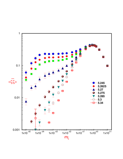
FIG. 1.: Semi-quenched condensate versus the valence quark mass $m_{\zeta}$ for two-flavor QCD [11] with a sea mass $m_{s}a=0.01$.

The bulk of the staggered lattice results can be understood from simple random matrix theory [7, 8, 9], if we note that for a bounded spectral density, the valence condensate is just

$$<\overline{\zeta}\zeta>(m_{\zeta})=\pi\varrho(im_{\zeta}).$$ (2)

which is just the spectral density for $\lambda=im_{\zeta}$. For staggered QCD fermions at zero temperature, the spectral distribution can be mapped on a chiral gaussian unitary ensemble, provided that the gauge configurations are sufficiently random. At finite temperature, this is equivalent to an assembly of Matsubara modes, each described by a gaussian unitary ensemble. At high temperature the only relevant modes are $\pm\pi T$, as suggested by the screening length measurements [3], and dimensional reduction [12]. We note that $\pi T$ is the minimum wavenumber $k=2\pi/\lambda$ of a massless quark mode on a circle of length $1/T$ with a wavelength $\lambda=2/T$. For massive quarks, the relevant modes are $\pm M(T)=\pm\sqrt{m_{s}^{2}+\pi^{2}T^{2}}$ [12]. With this in mind, a suggestive high temperature chiral random matrix model for two degenerate and massive flavors is

$${\bf Q}_{S}=\bigotimes_{\pm;f=1,2}\left(\left(\begin{array}[]{cc}0&\pm M(T)\\ \pm M(T)&0\end{array}\right)+\left(\begin{array}[]{cc}0&R\\ R^{\dagger}&0\end{array}\right)\right)$$ (7)

where each entry in (7) is $N\times N$ valued. The $R$’s are described by a gaussian unitary ensemble. The off-block-diagonal structure of (7) is suggestive of the chiral structure of $iD\!\!\!\!/$, which is preserved in the staggered fermion formulation. This is not the case for the Wilson fermions, as we discuss below. All the scales in (7) are given in units of $1/\Sigma=(100\,\,{\rm MeV})^{-1}$. Although (7) is well-motivated at high temperature, we will use it to investigate the temperature ranges around the critical temperature. This is a bit justified by the fact that the lattice simulations of the spatial screening lengths show a behavior that is consistent with the occurrence of the lowest Matsubara modes around $T\sim T_{c}$. For $m_{s}=0$, and in the case of one-flavor and a single Matsubara mode, (7) has been numerically investigated in [8].

The spectral distribution associated to (7) follows from the discontinuity of the pertinent solution to a cubic (Cardano) equation,

$$G^{3}(z)-2zG^{2}(z)+(z^{2}-M^{2}(T)+1)G-z=0$$ (8)

with $-\pi\varrho(\lambda)={\rm Im}G(\lambda+i0)$, this was also observed in [9] for the massless case. The equation (8) follows readily from the law of addition of random plus deterministic matrices [10].

In Fig. 2, we show the behaviors of the valence quark condensate for two choices of the sea quark masses, $m_{s}=0$ and $0.1$, and various $\beta$ (temperature) values as obtained from the Cardano solution (8). In physical units, $m=0$ and $10$ MeV. We have identified $\beta$ with $T$, through

$$\pi(T-T_{c})=(\beta-\beta_{c})$$ (9)

with the critical temperature $T_{c}$ in the chiral random matrix model and $\beta_{c}=5.275$ as suggested by the lattice calculations [11]. The transition in the chiral random matrix model is mean-field in character (large $N$). For $m_{s}=0.1$ (10 MeV) the random matrix model seems to follow qualitatively well the lattice results for $m_{s}a=0.01$ (6 MeV), except for $m_{\zeta}\leq 10^{-5}$, where the spectrum becomes sensitive to the finite size of the lattice, as illustrated by the bending of the upper curves. Finite size effects set in when the pion Compton wavelength becomes comparable to the lattice size. Using the PCAC relation this implies that $m_{\zeta}<\overline{\zeta}\zeta>\geq 1/N_{c}V_{4}$. For $V_{4}=4\times 16^{3}$, this puts a lower bound on the valence mass $m_{\zeta}\geq 10^{-4}$, which is about consistent with the lattice results. We note that the above interpretation of the finite temperature lattice simulation is different from the zero temperature universality argument used in [13], but in qualitative agreement with the finite-N numerical analysis carried in [8], in the massless case.

FIG. 2.: Semi-quenched condensate versus the valence quark mass $m_{\zeta}$ for two-flavor QCD, obtained from eq.(2) with the Cardano solution of eq.(8), for the sea quark masses $m_{s}=0$ (upper) and $m_{s}=0.1$ (lower).

We note that the reading of the critical temperature $\beta_{c}$ depends sensitively on the value of the sea quark mass, as can be seen by comparing the upper and lower curves on Fig. 2. For $m_{s}=0$, the critical temperature is $\beta=5.275$ (fifth line from the top), whereas for $m_{s}=0.1$, the critical value is $\beta=5.27$ (the fourth line from the top). In the random matrix model (Cardano solution), the dependence of the critical temperature on the sea quark mass is simply $\Delta\beta_{c}=\sqrt{1-m_{s}^{2}}$. Both lines have the same critical exponent $\delta=3$ (mean-field). This result was first established in [8]. For $\beta=5.275$, $<{\overline{\zeta}}\zeta>\sim m_{\zeta}^{0.33}$. For $\beta=5.34$, $<{\overline{\zeta}}\zeta>=8m_{\zeta}$. These values are to be contrasted with the ones quoted by Chandrasekharan and Christ [11], namely $<{\overline{\zeta}}\zeta>\sim m_{\zeta}^{0.6}$ for $\beta=5.275$, and $<{\overline{\zeta}}\zeta>\sim m_{\zeta}^{0.98}$ for $\beta=5.34$. The closeness of the latter to the random matrix result, suggests perhaps an underestimation of the critical exponent $\delta=5/3$ [11] in comparison with the mean-field one $\delta=3$, possibly due to the large finite sizes effects mentioned above as visible in Fig. 1 (dropping plateau’s for small masses). We recall that a two-flavor simulation of QCD using finite-temperature cumulants yields $\delta$ in the range 4-5 [14], hence closer to the mean-field result.

The fact that the semi-quenched condensate appears to vanish linearly with the valence quark mass $m_{\zeta}$ in the high temperature phase ($\beta>\beta_{c}$) prompted the Columbia group to analyze the asymmetry [11]

$$\omega=4m^{2}\int_{0}^{\infty}d\lambda\ \frac{\varrho(\lambda)}{(\lambda^{2}+m^{2})^{2}}$$ (10)

between the isotriplet and its axial partner. For a bounded spectrum , this expression reduces to

$$\omega=\frac{\pi\varrho(im)}{m}\ -\frac{\partial}{\partial m}\pi\varrho(im)\$$ (11)

Below the critical temperature and as $m$ goes to zero, the first term diverges (pion pole), while the second term approaches zero (plateau), provided that $\varrho(im)$ does not develop a low fractional dependence on the sea quark mass (set equal to the valence one). Above the critical temperature, the first term vanishes for any value of the mass $m$, which is followed by an infinite jump in $\omega$ at the critical temperature. For finite values of the mass $m$ this jump is smeared out.

Figure 3a shows the behavior for the Cardano solution with $m=0.005$ (0.5 MeV). Figure 3b shows the same curve for $ma=0.01$ (6 MeV) as obtained by Chandrasekharan and Christ on a $16^{3}\times 4$ lattice with staggered fermions [11]. The similarity is striking, although the mass scales are different. The fact that in the random matrix model, $\varrho(im)$, does not develop a low fractional dependence on $m$ is traced back to the structure of the thermal masses (T-regulated). We recall that the random matrix model considered here has no bearing on the axial-singlet anomaly. Its discussion in the context of random matrix models goes outside the scope of this work.

FIG. 3.: (a) Results from the random matrix model for $m=0.005$ in units of $\Sigma=1$. (b) results for staggered fermions on a $16^{3}\times 4$ lattice with $ma=0.01$ [11].

3.    Wilson fermion formulations are more natural to use for three-flavor QCD. Recently Kalkreuter has performed detailed lattice simulations with Wilson fermions for two-color and two-flavor QCD [15]. His results are in qualitative agreement with random matrix theory [16, 10] for the bulk spectrum. The issue with Wilson fermions, however, is that the Wilson terms needed to eliminate the lattice doublers break explicitly chiral symmetry. It is however expected, that in the continuum limit the breaking is mild enough (irrelevant operators) to allow for a full restoration of chiral symmetry, modulo mass terms.

In terms of chiral random matrix models, the pertinent ensemble for investigating Wilson fermions for QCD is the gaussian unitary ensemble , provided that the quarks are in the fundamental representation. In the presence of Wilson r-terms, the Dirac operator is only hermitean. It is not block-off-diagonal (chiral). Randomness, however, is sufficient to cause the spectral distribution to develop a non-vanishing value at zero virtuality and in the chiral limit. So, although the spectrum is not paired, the distribution is even. This is easily understood if the diagonal disorder (r-terms) is not large enough [10]. In fact, this can be easily investigated by considering a linear combination of two chiral random matrix models. One with off-diagonal randomness (chiral) plus one with diagonal randomness (r-terms) [18].

For three flavors, we define the hermitean Dirac operator ${\bf Q}={\displaystyle\otimes_{f}}\gamma_{5}(D\!\!\!\!/+m_{f})$, with $f=u,d,s$. Here ${\bf Q}$ is the Dirac $Hamiltonian$ in five-dimensions. The Dirac matrix $\gamma_{5}$ plays the role of $\beta$-Dirac matrix in (3+1) dimensions. On a cylinder, the pertinent random matrix model for spatially constant Wilson modes is

$${\bf Q}_{W}=\bigotimes_{f=u,d,s}\left(\left(\begin{array}[]{cc}m_{f}&\partial_{\tau}\\ -\partial_{\tau}&-m_{f}\end{array}\right)+{\bf R}\right)$$ (14)

where $\partial_{\tau}$ is the $\tau$-derivative on a cylinder of length $\beta=1/T$, and ${\bf R}$ a $\tau$-independent random matrix with a block structure specified by eq.(18) below. Equation (14) is defined with anti-periodic boundary conditions. It is diagonal in frequency space using

$$\psi(\tau)=\sum_{n}e^{i\omega_{n}\tau}\psi_{n}$$ (15)

where $\omega_{n}=(2n+1)\pi T$ are the usual Matsubara frequencies. Here $\psi(\tau)$ is an $N$-dimensional vector for each of the three flavors: up, down and strange. For each Matsubara frequency, and for each flavor (14) describes a set of $N$ fermions, with a hermitean Hamiltonian

$${\bf Q}_{n}^{f}=\left(\begin{array}[]{cc}m_{f}&i\omega_{n}\\ -i\omega_{n}&-m_{f}\end{array}\right)+\bigg{(}\ \mbox{$\displaystyle R^{f}_{n}$}\ \,\bigg{)}$$ (18)

This is a the sum of a deterministic and a random piece. Each entry in the first matrix is $N\times N$ valued. The random matrix is $2N\times 2N$ valued. In terms of (18), eq. (14) is block-diagonal in frequency and in flavor space,

$${\bf Q}_{W}=\bigotimes_{f=u,d,s}\bigotimes_{n=-\infty}^{+\infty}{\bf Q}_{n}^{f}$$ (19)

The random distributions for each Matsubara mode are decoupled, each with a weight

$$P({R_{n}})=\frac{1}{Z}\exp[-2N{\rm Tr}V({R_{n}})]$$ (20)

This is a direct consequence of our assumption that ${\bf R}$ in (14) is $\tau$-independent. If we were to relax this condition, then the random matrix may cause the Matsubara modes to couple [18]. In this paper, $V$ will be chosen gaussian, although polynomial weights are also possible [19]. The resolvent of (19) is

$$G(z)=\frac{1}{2NN_{f}N_{*}}\left<{\rm Tr}\frac{1}{z-{\bf Q}}\right>$$ (21)

The averaging is carried with the distribution (20). In terms of (21) the spectral distribution associated to (14)

$$\nu(\lambda)=\frac{1}{2N_{f}NN_{*}}\sum_{n=-\infty}^{+\infty}\sum_{f=u,d,s}{\rm Tr}_{2N}\,\delta(\lambda-{\bf Q}_{n}^{f})$$ (22)

is related to the discontinuity of $G(z)$ through the real axis

$$\nu(\lambda)=-\frac{1}{\pi}\,{\rm Im}G(z=\lambda+i0)$$ (23)

Equation (22) involves the sum over a large number of Matsubara modes, with $N_{*}=\sum_{n}$.

Using either the law of addition of random matrices [10, 20] or diagrammatic techniques [21], it follows that in large $N$ the resolvent $G(z)$ is

$$G(z)=\frac{1}{N_{f}N_{*}}\sum_{n,f}G_{n}^{f}(z)$$ (24)

where each of the $G_{n}^{f}(z)$ satisfying Pastur’s equation [22]

$$G_{n}^{f}(z)=\frac{1}{2}\left(\frac{1}{z-G_{n}^{f}(z)-{\bf M}_{n}^{f}}+\frac{1}{z-G_{n}^{f}(z)+{\bf M}_{n}^{f}}\right)$$ (25)

is a 2$\times$2 diagonal matrix, with $M_{n}^{f}(T)=\sqrt{m_{f}^{2}+\omega_{n}^{2}}$.

At high temperature, only few modes contribute to (24), $i.e.$ $\omega_{0}=\omega_{-1}=\pi T$. Taking $m_{u}\sim m_{d}$, the problem reduces to

$$G(z) = \frac{\alpha}{2}G^{u}(z)+\frac{(1-\alpha)}{2}G^{s}(z)$$ (26)

with $\alpha=1-1/N_{f}$, $N_{f}=3$ and $G^{f}(z)$ defined by (25). (26) is a combination of three third order algebraic equation (Cardano class) [10], for the resolvent $G(z)$.

The spectral density follows from the discontinuity of $G(z)$ along the imaginary axis (23). In the chiral limit, the discontinuity is related to the chiral condensate through the Banks-Casher argument,

$$<\bar{q}q>={\rm Im}\,\,G(z=i0)\,\,\,.$$ (27)

Although (26) was derived in the high temperature limit, we expect it to be rather accurate near the critical points because of universality. Indeed, at the critical point and in large $N$ only symmetry is relevant [23]. Below, we will provide an analysis of the spectral distribution associated to (26).

4.    The explicit solution of the third order equation is available in algebraic form, and was discussed in [10]. The combination of several third order equations allows for a rich phase structure. In the case of two light and one heavy flavors, the spectrum should exhibit at most four phases $P_{1},P_{2},P_{3}$ and $P_{4}$. The support of the spectral function may consists of one, two, three or four disconnected arcs, depending on the choice of the external parameters $m_{u}$, $m_{s}$, and $T$.

Figure 4 shows the behavior of the spectral function for the physical choice of $m_{u}=m_{d}=0.075,m_{s}=1.5$. All dimensionfull quantities are measured in units of $\Sigma=1$. In physical units, $m_{u}=m_{d}=7.5$MeV and $m_{s}=150$MeV. At zero temperature, the system is in the $P_{1}$ phase, and the value at zero virtuality ($\lambda=0$) corresponds to a non-zero condensate. The mass of the strange quark is 20 times higher, therefore the spectrum feels it by developing two symmetric shoulders. The mass is not high enough, however, to provide the decoupling of the strange quark ($P_{3}$ phase), with symmetric and disconnected humps. The effect of the temperature is to quench the maximum at the origin. At the critical temperature $T_{*}$, the quarks localize, resulting into a transition from $P_{1}\rightarrow P_{2}$. For increasing $T$, the thermal quark modes contribute democratically to the spectral distribution, $M_{u}=\sqrt{m_{u}^{2}+\pi^{2}T^{2}}\rightarrow\pi T$, $M_{s}=\sqrt{m_{s}^{2}+\pi^{2}T^{2}}\rightarrow\pi T$.

FIG. 4.: Spectral function for Wilson fermions with $m_{u}=m_{d}=0.075$ and $m_{s}=1.5$.

FIG. 5.: Spectral function for Wilson fermions with $m_{u}=m_{d}=0.075$ and $m_{s}=5$.

Figure 5 shows the same spectral distribution as Fig. 4, but this time for a large strange quark mass $m_{s}=5$, or $m_{s}=500$ MeV in physical units. The two additional humps at $T=0$ are just the delocalized strange quarks. An analysis of Cardano’s solutions show that the critical value for which this happens is $2m_{s}^{2}=11+\sqrt{125}$ for $m_{u}=0$. Here, the initial spectrum is in the $P_{3}$ phase. The effects of the temperature is to cause localization of the light quarks, first transition, from $P_{3}$ to $P_{4}$, resulting in the vanishing of the density of states at zero virtuality. This is followed by a second transition at higher temperature $T_{**}$ from $P_{4}$ to $P_{2}$ in which all the three flavors become thermally heavy.

Figure 6 shows the same spectral distribution for three large but comparable masses, $m_{u}=m_{d}=2$ and $m_{s}=4$. There is no phase transition, the system is always in the heavy (localized) phase $P_{2}$. There is no accumulation of quark states at zero virtuality. The thermal effects cause the localization to shift from the Compton wavelength to the thermal wavelength.

FIG. 6.: Spectral function for Wilson fermions with $m_{u}=m_{d}=2$ and $m_{s}=4$.

Figure 7 shows yet another choice of heavy quark masses $m_{u}=m_{d}=2$ and $m_{s}=6$, for which the spectral distribution undergoes a phase transition from $P_{4}$ to $P_{2}$. At low temperature the quarks are massive but distinct, at high temperature the distinction is washed out by temperature.

FIG. 7.: Spectral function for Wilson fermions with $m_{u}=m_{d}=2$ and $m_{s}=6$.

The spectra discussed above for the random matrix model, allow for an assessment of the critical lines (phase diagram) in terms of the end-points of the spectral distribution. The equations for the end-points are given by a polynomial equation that is always one degree lower than the one following from Pastur’s equation. This is best described using Blue’s functions [20], i.e. functional inverses of Green’s functions. Generically, the Blue’s function associated to the Green’s function $G(z)$ is given by

$$B(G(z))=z$$ (28)

The substitution $z\rightarrow B(z)$ and the use of (28) in Pastur’s equation (26) yield the pertinent equation for the Blue’s functions. Since the Green’s functions behave as $\sqrt{A-z}$ when $z$ approaches the endpoint $A$, then

$$\frac{dG}{dz}|_{end-point}=\infty\,\,\,\leftrightarrow\,\,\,\,\frac{dB}{dz}|_{end-point}=0$$ (29)

For our case, this yields a quadratic equation [10]. The end points are explicitly given by

$$A_{f}^{\pm}=\frac{1}{\sqrt{2}}\sqrt{1+2M_{f}^{2}\pm\sqrt{1+8M_{f}^{2}}}\frac{3\pm\sqrt{1+8M_{f}^{2}}}{1\pm\sqrt{1+8M_{f}^{2}}}$$ (30)

for all masses and temperatures. In the case of Figure 5 and 7, the transition from $P_{4}$ to $P_{2}$ is defined as $A_{u}^{+}=A_{s}^{-}$. In the high mass (temperature) limit this condition is equivalent to $M_{s}(T_{**})-M_{u}(T_{**})=2\sqrt{2}$. At zero virtuality the spectral distribution vanishes for $\pi T_{*}=\sqrt{1-m_{u}^{2}}$.

5.       We have shown that the chiral gaussian unitary ensemble for two massive flavors and finite temperature, allows for a quantitative description of the recent simulations by Chandrasekharan and Christ using staggered fermions. The agreement with the random matrix model at $\beta=5.34$ and higher suggests that the fit to the lattice data with $\delta=5/3$ may be underestimating the critical exponent at $\beta=5.275$ in comparison with the mean-field result by about a factor of two. We have also provided a qualitative understanding of the lattice anomalous symmetry breaking effect in a chiral random matrix model without the axial-singlet anomaly, albeit with a small sea quark mass.

We have suggested that in the chiral limit the gaussian unitary ensemble is the pertinent random ensemble for investigating Wilson fermions in QCD. We have explicitly shown that the problem of three flavor QCD in the Wilson formulation is amenable to a random plus deterministic problem for few Matsubara modes. We have used arguments at high temperature to unravel a number of properties of the spectral distribution for the hermitean Dirac operator (Hamiltonian in five dimensions). QCD with two light and one heavy flavor exhibits a spontaneously broken phase at low temperature, and a localized phase at high temperature. The localization is determined by the thermal wavelength. For QCD with massive flavors, the localization is a competitive effect between the thermal wavelength and the Compton wavelength.

We have explicitly used the end-points of the Dirac spectrum to construct the critical lines for massive QCD at finite temperature. The critical lines (phase diagrams) were shown to follow from a quadratic equation following from the Blue’s function. Given the qualitative agreement noted between our results, and the staggered fermion calculations, we look forward to a detailed comparison with future simulations using Wilson fermions for full QCD. We note, however, that our analysis does not account for the axial-singlet anomaly. Its role in the context of random matrix models will be discussed elsewhere.

The phase transitions discussed here are all mean-field in character. This is unavoidable in the large $N$ analysis performed here. The quantitative similarities between the Columbia results at finite temperature and the random matrix results, suggest that the phase transition in quarkish QCD may be characterized by a narrow Ginzburg window (perhaps of order $1/N$), thereby asserting the lore of mean-field exponents. Within the Ginzburg window scaling arguments and universality should hold [5].

The spectral distributions we have discussed here are of course amenable to finite $N$ corrections. This could be discussed either in the context of the corrections to Pastur’s equations or using diagrammatic techniques. Also, specific level correlations can be discussed either in the staggered formulation, or the Wilson one, both for massive QCD and finite temperature. These and other issues will be discussed elsewhere.

Acknowledgments This work was supported in part by the US DOE grant DE-FG-88ER40388, by the Polish Government Project (KBN) grant 2P03B19609 and by the Hungarian Research Foundation OTKA.

REFERENCES

- [1] K. Kanaya, ”Finite Temperature QCD on the Lattice”, Nucl. Phys. B (1996).
- [2] Y. Iwasaki, Nucl. Phys. (Proc. Suppl.) B42 (1995) 96.
- [3] C. DeTar, Nucl. Phys. (Proc. Suppl.) B42 (1995) 73.
- [4] M.A. Nowak, M. Rho and I. Zahed, Chiral Nuclear Dynamics, World-Scientific (1996), in print
- [5] R.D. Pisarski and F. Wilczek, Phys. Rev. D29 (1984) 338.
- [6] See e.g., C.E. Porter, Statistical Theories of Spectra: Fluctuations, Academic Press, New York, 1965; M.L. Mehta, Random Matrices, Academic Press, New York, 1991.
- [7] E.V. Shuryak and J.J.M. Verbaarschot, Nucl. Phys. A560 (1993) 306. J.J.M. Verbaarschot and I. Zahed, Phys. Rev. Lett. 70 (1993) 3852.
- [8] A.D. Jackson and J.J.M. Verbaarschot, “ A random matrix model for chiral symmetry breaking”, SUNY-NTG-95/26, eprint hep-ph/9509324.
- [9] M.A. Stephanov, “Chiral symmetry at finite T, the phase of Polyakov loop and the spectrum of the Dirac operator”, eprint hep-lat/9601001.
- [10] M.A. Nowak, G. Papp and I. Zahed, “QCD-inspired spectra from Blue’s functions”, e-print hep-ph/9603348.
- [11] S. Chandrasekharan and N. Christ, “Dirac Spectrum, Axial Anomaly and the QCD Chiral Phase Transition”, eprint hep-lat/9509095.
- [12] T.H. Hansson and I. Zahed, Nucl. Phys. B374 (1992) 117; G.E. Brown et al., Phys. Rev. D45 (1992) 3169; T.H. Hansson, M. Sporre and I. Zahed, Nucl. Phys. B427 (1994) 545.
- [13] J.J.M. Verbaarschot, Phys. Lett. B368 (1996) 137.
- [14] F. Karsch and E. Laermann, “Susceptibilities, the specific heat and a cumulant in two-flavor QCD”, BI-TP 94-29.
- [15] T. Kalkreuter, “Numerical analysis of the spectrum of the Dirac operator in four-dimensional gauge fields”, eprint hep-lat/9511009.
- [16] J. Jurkiewicz, M.A. Nowak and I. Zahed, “Dirac spectrum in QCD and quark masses”, e-print hep-ph/9603308.
- [17] J.J.M. Verbaarschot, in Continuous Advances in QCD, Ed. A.V. Smilga, World Scientific (1994).
- [18] M.A. Nowak, G. Papp and I. Zahed, in preparation.
- [19] E. Brezin, S. Hikami and A. Zee, ”Oscillating density of states near zero energy for matrices made of blocks with possible application to the random flux problem”, eprint cond-mat/9511104.
- [20] A. Zee, “Law of addition in random matrix theory”, eprint cond-mat/9602146.
- [21] E. Brezin and A. Zee, Phys. Rev. E49 (1994) 2588.
- [22] L.A. Pastur, Theor. Mat. Phys. (USSR) 10 (1972) 67.
- [23] M.A. Nowak and I. Zahed, in preparation.