WEAK-SCALE SUPERSYMMETRY:
THEORY AND PRACTICE

These lectures contain an introduction to the theory and practice of weak-scale supersymmetry. They begin with a discussion of the hierarchy problem and the motivation for weak-scale supersymmetry. They continue by developing the coset approach to superfields. They use superfield techniques to construct the minimal supersymmetric version of the standard model and to discuss soft supersymmetry breaking and its implications. The lectures end with a brief survey of expectations for future collider experiments.

1.  Introduction and Motivation

During the past decade, the standard model of particle physics has been tested to a remarkable degree of accuracy. Precision measurements have confirmed its predictions to the level of radiative corrections $[{\bf?}]$ – $[{\bf?}]$. With the discovery of the top quark, the matter sector of the standard model stands essentially complete. All that remains is to find the Higgs, the missing ingredient of the standard model.

Such is the conventional wisdom. In reality, the situation is not so simple. While there is no doubt that precision tests have challenged the standard model as never before, the status of the Higgs is still open to question. At present, the experimental limits do not reveal much about the Higgs and its properties $[{\bf?}]$. Indeed, many theorists believe that the search for the Higgs will uncover new physics that is even more interesting than that associated with the Higgs itself.

These beliefs are motivated by a host of theoretical problems with the ordinary standard model. Perhaps the most compelling is the so-called hierarchy problem, the famous instability of the Higgs mass under quadratically divergent radiative corrections $[{\bf?}]$. These lectures will explain the hierarchy problem and use it to motivate a new symmetry – called supersymmetry – that might become manifest at the TeV scale $[{\bf?}]$ – $[{\bf?}]$. If supersymmetry is correct, it will lead to a rich new spectroscopy in the years to come.

It is in this spirit that these lectures will present an introduction to weak-scale supersymmetry. (They will not discuss physics at the Planck scale.) They will develop the necessary supersymmetric technology and use it to construct the minimal supersymmetrized version of the standard model. They will also prepare the ground for the lectures of Tata $[{\bf?}]$ and Seiberg $[{\bf?}]$.

We shall start by discussing the hierarchy problem. To understand the issues involved, we will consider a toy model with one complex scalar, $A$, and one Weyl fermion, $\chi$. We take the Lagrangian to be as follows,

$${\cal L}\;= - \partial_{m}A^{*}\partial^{m}A\;-\;i\bar{\chi}\bar{\sigma}^{m}\partial_{m}\chi$$ (1.1)

$$- {1\over 2}\,M_{F}\,\chi\chi\;-\;{1\over 2}\,M_{F}\,\bar{\chi}\bar{\chi}\;-\;\lambda_{F}\,A\chi\chi\;-\;\lambda_{F}\,A^{*}\bar{\chi}\bar{\chi}$$

$$- M^{2}_{B}\,A^{*}A\;-\;\lambda_{B}\,(A^{*}A)^{2}\;,$$

where we use two component spinor notation, outlined in the Appendix.

Figure 1: The one-loop correction to the fermion mass is logarithmically divergent, and proportional to the fermion mass, $M_{F}$.

The Lagrangian (1.1) enjoys a global U(1) chiral symmetry,

$$A \rightarrow e^{-2i\alpha}\,A$$

$$\chi \rightarrow e^{i\alpha}\,\chi\;.$$ (1.2)

This symmetry is broken only by the fermion mass, $M_{F}$. Because of this symmetry, the one-loop fermion mass correction must contain at least one mass insertion, as shown in Fig. 1. Therefore the fermion mass correction is multiplicative, of the form

$$\delta M_{F}\;\simeq\;{\lambda_{F}^{2}\over 16\pi^{2}}\;M_{F}\;.$$ (1.3)

Equation (1.3) illustrates why fermion masses are said to be natural: they are stable under radiative corrections. Once $M_{F}$ is fixed at tree level, it is protected from large radiative corrections by the U(1) chiral symmetry $[{\bf?}]$.

Figure 2: The one-loop corrections to the boson mass contain two quadratically divergent contributions of opposite sign.

The boson mass, $M_{B}$, stands in contrast to the fermion mass. The boson mass is not protected by the chiral symmetry, so at one loop, it receives additive contributions, as shown in Fig. 2. By power counting, one finds that the scalar mass renormalizations are quadratically divergent,

$$\delta M_{B}^{2}\;=\;{\lambda_{B}\over 16\pi^{2}}\,\Lambda^{2}\;-\;{\lambda_{F}^{2}\over 16\pi^{2}}\,\Lambda^{2}\;,$$ (1.4)

where $\Lambda$ is a large ultraviolet cutoff, and the minus sign comes from the fermion loop. Equation (1.4) illustrates why light scalar masses are not natural. Their tree-level values are not stable; they receive large, quadratically divergent, radiative corrections $[{\bf?}]$.

For the case of the standard model, this analysis applies to the scalar Higgs boson, $h$. In the standard model, the Higgs mass, $M_{h}$, is of order the $W$ mass, $M_{W}$, and is proportional to a vacuum expectation value, $v$. The vev $v^{2}$ receives quadratically divergent radiative corrections. This means that the natural scale for the Higgs mass is of order the cutoff, $\Lambda$, which is presumably the Planck scale, $M_{P}$, or the unification scale, $M_{\rm GUT}$.

Of course, technically speaking, there is nothing wrong with this instability. It is certainly possible to adjust the one-loop counterterms so that they cancel the quadratic divergence. However, this cancellation requires an exquisite fine tuning of one part in $10^{17}$ to maintain the hierarchy $M_{W}\ll M_{P}$. This fine tuning is not natural; it lies at the heart of the hierarchy problem.

The toy model discussed above illustrates the hierarchy problem, but it also hints at a possible resolution. From eq. (1.4) we see that it is possible for the quadratic divergences to cancel between the bosonic and fermionic loops. For the case at hand, this requires that $\lambda_{B}$ be related to $\lambda_{F}^{2}$. More generally – and to ensure that the cancellation persists to all orders – it requires a symmetry, called supersymmetry.

During the course of these lectures, we shall see that supersymmetry protects the hierarchy $M_{W}\ll M_{P}$ by canceling all dangerous quadratic divergences. In the supersymmetric standard model, this requires a doubling of the particle spectrum. For every particle that has been discovered, supersymmetry predicts another that has not. The extra particles circulate in loops and protect the hierarchy from destabilizing divergences $[{\bf?}]$.

In what follows we will also review present expectations for the supersymmetric particle spectrum. We will see that current limits pose no serious constraints on the parameter space. We will also see that the next generation of accelerators, including the Fermilab Main Injector, LEP 200, and a possible higher-luminosity Tevatron, will open a new era in supersymmetric particle searches. These accelerators will – for the first time – begin to probe significant regions of the supersymmetric parameter space. And with the advent of the LHC, we shall find that weak-scale supersymmetry will be placed to a definitive test.

2.  Supersymmetry and the Wess-Zumino Model

Supersymmetric field theories are based on the following algebra $[{\bf?}]$,

$$\{Q_{\alpha},\;\bar{Q}_{\dot{\alpha}}\} = 2\sigma_{\alpha{\dot{\alpha}}}^{m}P_{m}$$

$$\{Q_{\alpha},\;Q_{\beta}\} = \{\bar{Q}_{\dot{\alpha}},\;\bar{Q}_{\dot{\beta}}\}\;=\;0$$

$$\left[P_{m},\;Q_{\alpha}\right] = \left[P_{m},\;\bar{Q}_{\dot{\alpha}}\right]\;=\;0$$

$$\left[P_{m},\;P_{n}\right] = 0\;.$$ (2.1)

This is a graded Lie algebra because it contains bosonic and fermionic generators. (In four dimensions, there can be up to eight fermionic generators $Q^{A}_{\alpha}$, with $A=1,...,8.$ We shall restrict our attention to the simplest case, with only one generator, $Q_{\alpha}$.)

The supersymmetry algebra relates particles of different spins. It is a nontrivial extension of the usual Poincaré spacetime symmetry. Indeed, the local version of supersymmetry leads to an extension of Einstein gravity, called supergravity $[{\bf?}]$. Supergravitational effects are suppressed by powers of $M_{P}$, and will not concern us here.

Supersymmetry would be a mathematical curiosity were it not for the fact that it can be implemented consistently in local, relativistic quantum field theory. The supersymmetry charges, $Q_{\alpha}$, can be obtained as Noether charges associated with a conserved fermionic Noether current, $J^{m}_{\alpha}$,

$$Q_{\alpha} = \int d^{3}x\;J^{0}_{\alpha}$$

$$\partial_{m}J^{m}_{\alpha} = 0\;.$$ (2.2)

The simplest supersymmetric field theory is the Wess-Zumino model $[{\bf?}]$, the supersymmetric generalization of the toy model discussed above. The Wess-Zumino model involves one Weyl fermion, $\chi$, and two complex scalar fields, $A$ and $F$. The infinitesimal supersymmetry transformations are as follows,

$$\delta_{\xi}A = (\xi Q+\bar{\xi}\bar{Q})\times A\;=\;\sqrt{2}\,\xi\chi$$

$$\delta_{\xi}\chi = (\xi Q+\bar{\xi}\bar{Q})\times\chi\;=\;i\sqrt{2}\,\sigma^{m}\bar{\xi}\partial_{m}A\;+\;\sqrt{2}\,\xi F$$

$$\delta_{\xi}F = (\xi Q+\bar{\xi}\bar{Q})\times F\;=\;i\sqrt{2}\,\bar{\xi}\bar{\sigma}^{m}\partial_{m}\chi\;,$$ (2.3)

where $\xi$ is an anticommuting parameter. It is a useful exercise to check that the supersymmetry transformations close into the supersymmetry algebra,

$$[\delta_{\eta},\delta_{\xi}]\,A\;=\;-\;2i\,(\eta\sigma^{m}\bar{\xi}-\xi\sigma^{m}\bar{\eta})\;\partial_{m}A\ ,$$ (2.4)

and likewise for $\chi$ and $F$.

The Wess-Zumino model has the following Lagrangian $[{\bf?}]$,

$${\cal L}\;=\;{\cal L}_{0}\;+\;{\cal L}_{1}\;,$$ (2.5)

where

$${\cal L}_{0}\;=\;-\;\partial_{m}A^{*}\partial^{m}A\;-\;i\bar{\chi}\bar{\sigma}^{m}\partial_{m}\chi\;+\;F^{*}F$$ (2.6)

and

$${\cal L}_{1}\;=\;M\,(AF\;-\;{1\over 2}\;\chi\chi)\;+\;\lambda\,(A^{2}F-A\chi\chi)\;+\;{\rm h.c.}$$ (2.7)

This Lagrangian is invariant (up to a total derivative) under the supersymmetry transformations (2.3).

The equations of motion for $A,\;\chi$ and $F$ can be derived in the usual way. The fields $A$ and $\chi$ describe propagating, physical particles. The field $F$ does not propagate. Its equation of motion is algebraic,

$${\partial{\cal L}\over\partial F}\;=\;F^{*}+M\,A+\lambda\,A^{2}\;=\;0\;,$$ (2.8)

so $F$ can be eliminated using (2.8). One finds

$${\cal L} = -\;\partial_{m}A^{*}\partial^{m}A\;-\;i\,\bar{\chi}\bar{\sigma}^{m}\partial_{m}\chi\;-\;{\cal V}(A^{*},A)$$ (2.9)

$$-\;{1\over 2}\,M\,\chi\chi\;-\;{1\over 2}\,M\,\bar{\chi}\bar{\chi}\;-\;\lambda\,A\,\chi\chi\;-\;\lambda^{*}A^{*}\bar{\chi}\bar{\chi}\;,$$

where the potential

$${\cal V}(A^{*},A)\;=\;|\,M\,A\;+\;\lambda\,A^{2}\,|^{2}$$ (2.10)

is positive definite.

The Lagrangian (2.9) is the supersymmetric generalization of the toy model discussed before. It describes two physical fields: one complex scalar and one Weyl fermion, both of mass $M$. The fields interact via Yukawa and scalar couplings. For the case at hand, $\lambda_{F}=\lambda$ and $\lambda_{B}=\lambda^{*}\lambda$. These choices are fixed by supersymmetry; they ensure that all quadratic divergences cancel between bosonic and fermionic loops.

The equality of boson and fermion masses is a general feature of supersymmetric field theories. It follows from the fact that $[P_{m},\;Q_{\alpha}]=[P_{m},\;\bar{Q}_{\dot{\alpha}}]=0$, which implies that $P^{2}$ is a Casimir operator of the supersymmetry algebra. The absence of supersymmetric partners for the observed particles means that supersymmetry must be broken in the everyday world.

3.  Coset Construction

The Wess-Zumino model is instructive because it contains the essential elements of supersymmetry. However, it is just one example of a supersymmetric field theory, and we would like to be able to construct more at will. In this section we will develop a formalism which permits the construction of manifestly supersymmetric quantum field theories.

In ordinary field theory, Poincaré symmetry is represented by differential operators on scalar, spinor and vector fields. Since supersymmetry is a spacetime symmetry, it makes sense to represent supersymmetry on superfields, supersymmetric generalizations of ordinary fields. The supersymmetry generators act as differential operators on the superfields.

The systematic construction of superfields can be carried out using a generalization of the coset construction of Callan, Coleman, Wess and Zumino $[{\bf?}]$, and Volkov $[{\bf?}]$. The construction is rather involved, but it is so useful that we will present it in complete generality $[{\bf?}]$. In the next section we will specialize to the case of supersymmetry and superfields.

The coset construction proceeds as follows. We start with a group, $G$, of internal and spacetime symmetries, and partition the (hermitian) generators of $G$ into the following three classes:

• $\Gamma_{A}$, the generators of unbroken spacetime translations;

• $\Gamma_{a}$, the generators of spontaneously broken internal and spacetime symmetries; and

• $\Gamma_{i}$, the generators of unbroken spacetime rotations and unbroken internal symmetries.

The generators $\Gamma_{i}$ close into the stability group, $H$.

Given $G$ and $H$, we can construct the coset $G/H$. We can define the coset by an equivalence relation on the elements of $G$,

$$\Omega\;\sim\;\Omega\,h\ ,$$ (3.1)

with $\Omega\in G$ and $h\in H$. Therefore the coset can be pictured as in Fig. 3, as a section of a fiber bundle with total space, $G$, and fiber, $H$.

Figure 3: A schematic representation of the coset $G/H$. The full space represents the group $G$, while the vertical lines denote orbits under $H$. Note that a general $G$ transformation induces a compensating $H$ transformation to restore the section.

The definition (3.1) motivates us to parametrize the coset as follows,

$$\Omega\;=\;e^{iX^{A}\Gamma_{A}}\;e^{i\pi^{a}(X)\Gamma_{a}}\;.$$ (3.2)

Physically, the $X^{A}$ play the role of generalized spacetime coordinates, while the $\pi^{a}(X)$ are generalized Goldstone fields, defined on the generalized coordinates and valued in the set of broken generators $\Gamma_{a}$. There is one generalized coordinate for every unbroken spacetime translation, and one generalized Goldstone field for every spontaneously broken generator.

We define the action of the group $G$ on the coset $G/H$ by left multiplication,

$$\Omega\;\rightarrow\;g\,\Omega\;=\;\Omega^{\prime}\,h\;,$$ (3.3)

with $g\in G$. In this expression

$$\Omega^{\prime}\;=\;e^{iX^{\prime A}\Gamma_{A}}\;e^{i\pi^{\prime a}(X^{\prime})\Gamma_{a}}$$ (3.4)

and

$$h\;=\;e^{i\alpha^{i}(g,X,\pi)\Gamma_{i}}\ .$$ (3.5)

The group multiplication induces transformations on the coordinates $X^{A}$ and the Goldstone fields $\pi^{a}$:

$$X^{A} \rightarrow X^{\prime A}$$

$$\pi^{a}(X) \rightarrow \pi^{\prime a}(X^{\prime})\;.$$ (3.6)

These transformations realize the full symmetry group, $G$. In the general case, they are highly nonlinear functions of $g,\;\pi^{a}$ and $X^{A}$. By construction, they linearize on the stability group, $H$. Furthermore, the field $\pi^{a}$ transforms by a shift under the transformation generated by $\Gamma_{a}$. This confirms that $\pi^{a}$ is indeed the Goldstone field corresponding to the broken generator $\Gamma_{a}$.

An arbitrary $G$ transformation induces a compensating $H$ transformation along the fiber, as shown in eq. (3.3) and Fig. 3. This transformation can be used to lift any representation, $R$, of $H$, to a nonlinear realization of the full group, $G$,

$$\psi(X)\;\rightarrow\psi^{\prime}(X^{\prime})\;=\;D(h)\psi(X)\;.$$ (3.7)

Here $D(h)=\exp(i\alpha^{i}T_{i})$, where $\alpha^{i}$ was defined in eq. (3.5), and the $T_{i}$ are the hermitian generators of $H$ in the representation $R$.

Having defined a nonlinear realization of $G$, we are now ready to construct an invariant action. The task is made easier by identifying the vielbein, connection and covariant derivatives. These are the covariant building blocks that we will use to construct a $G$-invariant action.

The procedure is as follows. We first construct the Maurer-Cartan form, $\Omega^{-1}d\Omega$, where $d$ is the exterior derivative. The Maurer-Cartan form is valued in the Lie algebra of $G$, so it has the expansion

$$\Omega^{-1}d\Omega\;=\;i(\omega^{A}\Gamma_{A}\;+\;\omega^{a}\Gamma_{a}\;+\;\omega^{i}\Gamma_{i})\;,$$ (3.8)

where $\omega^{A},\;\omega^{a}$ and $\omega^{i}$ are a set of one-forms on the manifold parametrized by the coordinates $X^{A}$.

The Maurer-Cartan form transforms as follows under a rigid $G$ transformation,

$$\Omega \rightarrow g\;\Omega\;h^{-1}$$

$$\Omega^{-1}d\Omega \rightarrow h(\Omega^{-1}d\Omega)h^{-1}\;-\;dh\,h^{-1}\;.$$ (3.9)

Comparing with (3.8), we see that $\omega^{A}$ and $\omega^{a}$ transform covariantly under $G$, while $\omega^{i}$ transforms by a shift,

$$\omega\;\equiv\;\omega^{i}\Gamma_{i}\;\rightarrow\;h\omega h^{-1}+i\,dh\,h^{-1}\;.$$ (3.10)

These transformations help us identify

$$\omega^{A}\;=\;dX^{M}\,E_{M}{}^{A}$$ (3.11)

as the covariant vielbein,

$$\omega^{a}\;=\;dX^{M}\,E_{M}{}^{A}D_{A}\pi^{a}$$ (3.12)

as the covariant derivative of the Goldstone field $\pi^{a}$, and

$$\omega^{i}\;=\;dX^{M}\,\omega_{M}^{i}$$ (3.13)

as the connection associated with the stability group, $H$.

With these building blocks, it is easy to construct an action invariant under the group $G$. The first step is to write all ordinary derivatives as covariant derivatives. For the Goldstone fields, these are the $D_{A}\pi^{a}$ introduced above. For the others, they are

$$D_{A}\psi\;=\;E_{A}{}^{M}\,(\partial_{M}\,+\,\omega^{i}_{M}T_{i})\,\psi\ ,$$ (3.14)

where $\omega^{i}_{M}$ is the $H$-connection (3.13), and the $T_{i}$ are the generators of $H$ in the representation $R$ of $\psi$.

Given the covariant derivatives, it is easy to write a $G$-invariant action. It is simply

$$S\;=\;\int d^{D}X\;\det E_{M}{}^{A}\;{\cal L}(\psi,\,D_{A}\psi,\,D_{A}\pi^{a})\;,$$ (3.15)

where ${\cal L}$ is a Lagrangian density, invariant under $H$. The coset construction ensures that the full action is automatically invariant under $G$.

This construction is very general – and very formal. To see how it works, let us consider the simplest possible case: Poincaré invariant field theory. In this case, $G$ is the Poincaré group, and $H$ its Lorentz subgroup. There are no Goldstone fields, so we identify

$$\Omega\;=\;e^{-iP_{a}x^{a}}\;,$$ (3.16)

where the $P_{a}$ are the usual momentum generators, and we replace $A$ by $a=1,...,4.$

We will study the most general Poincaré transformation,

$$g\;=\;e^{i(P_{a}c^{a}+J^{a}{}_{b}\lambda^{b}{}_{a})}\;,$$ (3.17)

where the $J^{a}{}_{b}$ generate the Lorentz group, $H$. The group transformation

$$\Omega\;\rightarrow\;\Omega^{\prime}\;=\;g\,\Omega\,h^{-1}$$ (3.18)

implies

$$x^{\prime a}\;=\;x^{a}\;-\;c^{a}\;+\;2\,\lambda^{a}{}_{b}x^{b}$$ (3.19)

and

$$h\;=\;e^{iJ^{a}{}_{b}\lambda^{b}{}_{a}}\;.$$ (3.20)

By definition, a scalar field $\phi$ transforms as a singlet under $H$,

$$\phi^{\prime}(x^{\prime})\;=\;\phi(x)\ .$$ (3.21)

For an infinitesimal transformation, this reduces to

$$\delta\phi(x) = \phi^{\prime}(x)\;-\;\phi(x)$$ (3.22)

$$= (c^{a}\;-\;2\,\lambda^{a}{}_{b}x^{b})\,\partial_{a}\phi(x)\;.$$

A spinor field $\chi$ transforms as follows under $H$,

$$\chi^{\prime}(x^{\prime})\;=\;D(h)\,\chi(x)$$ (3.23)

where $D(h)=\exp(\lambda^{ab}\sigma^{ab})$. For infinitesimal transformations, this becomes

$$\delta\chi(x) = (c^{a}\;-\;2\,\lambda^{a}{}_{b}x^{b})\,\partial_{a}\chi(x)$$ (3.24)

$$+\;\lambda^{ab}\sigma^{ab}\,\chi(x)\;,$$

as expected for a spinor field.

To find the invariant Lagrangian, we construct the Maurer-Cartan form, $\Omega^{-1}d\Omega=-idx^{a}P_{a}$. We extract the vielbein, $E_{m}{}^{a}=\delta_{m}{}^{a}$, and the connection, $\omega^{i}=0$. We see that the covariant derivative $D_{a}$ is just $\partial_{a}$. With these results, we are able to construct a Poincaré invariant action. We find

$$S\;=\;\int d^{4}x\;{\cal L}(\phi,\,\partial_{a}\phi,\,\psi,\,\partial_{a}\psi)\;,$$ (3.25)

where the Lagrangian density, ${\cal L}$, is invariant under the Lorentz group, $H$. Equation (3.25) is nothing but the usual Poincaré invariant action for quantum field theory – derived in the most sophisticated possible way!

4.  General Superfields

The coset construction is much too technical for the case of ordinary Poincaré-invariant field theory. It just reproduces what we already know. However, for the case of supersymmetry, the coset construction leads to something new: a manifestly supersymmetric technique for constructing supersymmetric quantum field theories $[{\bf?},{\bf?}]$.

In this section we shall see how this works. We will take $G$ to be the supergroup generated by the supersymmetry algebra (2.1). We take the group $H$ to be the Lorentz group, and we choose to keep all of $G$ unbroken. Therefore we have

$$\Omega\;=\;e^{i(-x^{a}P_{a}+\theta^{\alpha}Q_{\alpha}+\bar{\theta}_{\dot{\alpha}}\bar{Q}^{\dot{\alpha}})}\;,$$ (4.1)

where the generalized spacetime coordinates are $z=(x,\,\theta,\,\bar{\theta})$. The coordinates $\theta$ and $\bar{\theta}$ are Lorentz spinors, so we take them to anticommute

$$\{\theta^{\alpha},\;\theta^{\beta}\}\;=\;\{\bar{\theta}_{\dot{\alpha}},\;\bar{\theta}_{\dot{\beta}}\}\;=\;\{\theta^{\alpha},\;\bar{\theta}_{\dot{\beta}}\}\;=\;0\;.$$ (4.2)

We call the coordinates $(x,\,\theta,\,\bar{\theta})$ superspace.

A supersymmetry transformation is specified by the group element

$$g\;=\;e^{i(\xi^{\alpha}Q_{\alpha}+\bar{\xi}_{\dot{\alpha}}\bar{Q}^{\dot{\alpha}})}\;,$$ (4.3)

with anticommuting parameters $(\xi,\;\bar{\xi})$. The transformation

$$\Omega\;\rightarrow\;\Omega^{\prime}\;=\;g\Omega h^{-1}$$ (4.4)

induces the motion

$$x^{a} \rightarrow x^{a}\;+\;i\theta\sigma^{a}\bar{\xi}\;-\;i\xi\sigma^{a}\bar{\theta}$$

$$\theta^{\alpha} \rightarrow \theta^{\alpha}\;+\;\xi^{\alpha}$$

$$\bar{\theta}_{\dot{\alpha}} \rightarrow \bar{\theta}_{\dot{\alpha}}\;+\;\bar{\xi}_{\dot{\alpha}}$$ (4.5)

and

$$h\;=\;1\;.$$ (4.6)

Given these transformations, we define a scalar superfield $F(z)$ in analogy to (3.21),

$$F^{\prime}(z^{\prime})\;=\;F(z)\;.$$ (4.7)

Under an infinitesimal supersymmetry transformation, this reduces to

$$\delta_{\xi}F(z) = F^{\prime}(z)\;-\;F(z)$$ (4.8)

$$= (\xi^{\alpha}Q_{\alpha}\;+\;\bar{\xi}_{\dot{\alpha}}\bar{Q}^{\dot{\alpha}})\,F(z)\;,$$

where the differential operators $Q$ and $\bar{Q}$ are

$$Q_{\alpha} = {\partial\over\partial\theta^{\alpha}}\;-\;i\sigma^{m}_{\alpha{\dot{\alpha}}}\bar{\theta}^{\dot{\alpha}}\,\partial_{m}$$

$$\bar{Q}^{\dot{\alpha}} = {\partial\over\partial\bar{\theta}_{\dot{\alpha}}}\;-\;i\theta^{\alpha}\sigma^{m}_{\alpha{\dot{\beta}}}\epsilon^{{\dot{\beta}}{\dot{\alpha}}}\,\partial_{m}\;.$$ (4.9)

The anticommuting derivatives obey the relations

$${\partial\over\partial\theta^{\alpha}}\,\theta^{\beta} = \delta_{\alpha}^{\beta}$$

$${\partial\over\partial\theta^{\alpha}}\,\theta^{\beta}\theta^{\gamma} = \delta_{\alpha}^{\beta}\theta^{\gamma}\;-\;\theta^{\beta}\delta_{\alpha}^{\gamma}\;,$$ (4.10)

and similarly for $\bar{\theta}$. It is a useful exercise to check the differential operators $Q$ and $\bar{Q}$ close into the supersymmetry algebra:

$$\{Q_{\alpha},\;\bar{Q}_{\dot{\alpha}}\} = 2i\sigma_{\alpha{\dot{\alpha}}}^{m}\,\partial_{m}$$

$$\{Q_{\alpha},\;Q_{\beta}\} = \{\bar{Q}_{\dot{\alpha}},\;\bar{Q}_{\dot{\beta}}\}\;=\;0\;.$$ (4.11)

This ensures that superfields do indeed represent the supersymmetry algebra.

To find an invariant action, we compute the Maurer-Cartan form, $\Omega^{-1}d\Omega$. It is a useful exercise to extract the vielbein,

$$E_{M}{}^{A}\;=\;\pmatrix{\delta_{m}{}^{a}&0&0\crcr\vskip 3.0pt\cr-i\sigma^{a}_{\mu{\dot{\mu}}}\bar{\theta}^{\dot{\mu}}&\delta_{\mu}{}^{\alpha}&0\crcr\vskip 3.0pt\cr-i\theta^{\mu}\sigma^{a}_{\mu{\dot{\nu}}}\epsilon^{{\dot{\nu}}{\dot{\mu}}}&0&\delta^{\dot{\mu}}{}_{\dot{\alpha}}\crcr\vskip 3.0pt\cr}\ ,$$ (4.12)

and the $H$-connection,

$$\omega^{i}\;=\;0\;.$$ (4.13)

Then the covariant derivative of a scalar superfield is just

$$D_{A}F(z)\;=\;E_{A}{}^{M}\,\partial_{M}F(z)\;,$$ (4.14)

where the supersymmetric covariant derivatives are

$$D_{a} = \partial_{a}$$

$$D_{\alpha} = {\partial\over\partial\theta^{\alpha}}\;+\;i\sigma^{m}_{\alpha{\dot{\alpha}}}\bar{\theta}^{\dot{\alpha}}\,\partial_{m}$$

$$\bar{D}^{\dot{\alpha}} = {\partial\over\partial\bar{\theta}_{\dot{\alpha}}}\;+\;i\theta^{\alpha}\sigma^{m}_{\alpha{\dot{\beta}}}\epsilon^{{\dot{\beta}}{\dot{\alpha}}}\,\partial_{m}\;.$$ (4.15)

By construction, the supersymmetric covariant derivatives (anti)commute with the supersymmetry generators,

$$\{Q_{\alpha},\;D_{\beta}\}\;=\;\{\bar{Q}_{\dot{\alpha}},\;\bar{D}_{\dot{\beta}}\}\;=\;\{Q_{\alpha},\;\bar{D}_{\dot{\beta}}\}\;=\;\{\bar{Q}_{\dot{\alpha}},\;D_{\beta}\}\;=\;0\;.$$ (4.16)

They also obey the following structure relations

$$\{D_{\alpha},\;\bar{D}_{\dot{\alpha}}\} = -2i\,\sigma^{m}_{\alpha{\dot{\alpha}}}\,\partial_{m}$$

$$\{D_{\alpha},\;D_{\beta}\} = \{\bar{D}_{\dot{\alpha}},\;\bar{D}_{\dot{\beta}}\}\;=\;0\;.$$ (4.17)

To make contact with physics, we must extract $x$-dependent component fields from the superfields. This can be done by expanding the superfields in terms of $\theta$ and $\bar{\theta}$:

$$F(x,\theta,\bar{\theta}) = f(x)\;+\;\theta\varphi(x)\;+\;\bar{\theta}\bar{\phi}(x)$$ (4.18)

$$+\;\theta\theta\,m(x)\;+\;\bar{\theta}\bar{\theta}\,n(x)\ +\;\theta\sigma^{m}\bar{\theta}v_{m}(x)$$

$$+\ \theta\theta\bar{\theta}\bar{\lambda}(x)\ +\ \bar{\theta}\bar{\theta}\theta\psi(x)\ +\;\theta\theta\bar{\theta}\bar{\theta}\,d(x)\;.$$

The expansion terminates because $\theta$ and $\bar{\theta}$ anticommute. This implies that a given superfield contains a finite number of component fields.

The supersymmetry transformations of the component fields can be found from the supersymmetry transformations of the superfields,

$$\delta_{\xi}F(x,\theta,\bar{\theta}) = (\xi Q\ +\ \bar{\xi}\bar{Q})\,F(x,\theta,\bar{\theta})$$ (4.19)

$$= \delta_{\xi}f(x)\;+\;\theta\,\delta_{\xi}\varphi(x)\;+\;\bar{\theta}\,\delta_{\xi}\bar{\phi}(x)$$

$$+\;\theta\theta\,\delta_{\xi}m(x)\;+\;\bar{\theta}\bar{\theta}\,\delta_{\xi}n(x)\ +\;\theta\sigma^{m}\bar{\theta}\,\delta_{\xi}v_{m}(x)$$

$$+\ \theta\theta\bar{\theta}\,\delta_{\xi}\bar{\lambda}(x)\ +\ \bar{\theta}\bar{\theta}\theta\,\delta_{\xi}\psi(x)+\;\theta\theta\bar{\theta}\bar{\theta}\,\delta_{\xi}d(x)\;.$$

By construction, the component transformations close into supersymmetry algebra.

5.  Chiral Superfields

In this section we will write the Wess-Zumino model $[{\bf?}]$ in manifestly covariant form. Our results will serve as the first step towards constructing more general supersymmetric theories with spin-zero and spin-$\frac{1}{2}$ fields.

At first glance, it might seem simple to write down the Wess-Zumino model in terms of the superfields discussed in the previous section. However, the problem is harder than it first appears because a general scalar superfield contains far too many component fields. We must first reduce the number of component fields by imposing a covariant constraint.

It turns out that the right constraint is just $[{\bf?}]$

$$\bar{D}_{\dot{\alpha}}\Phi\;=\;0\;.$$ (5.1)

This defines the chiral superfield, $\Phi$. The constraint is consistent in the sense that it is covariant, and does not impose equations of motion on the component fields.

We can solve the constraint (5.1) by writing $\Phi$ as a function of $y$ and $\theta$, where

$$y^{m}\;=\;x^{m}\;+\;i\theta\sigma^{m}\bar{\theta}\;.$$ (5.2)

Since $\bar{D}\theta=\bar{D}y=0$, the field $\Phi(y,\theta)$ automatically satisfies the constraint (5.1).

To find the component fields, we expand $\Phi(y,\theta)$ in terms of $\theta$,

$$\Phi(y,\theta) = A(y)\;+\;\sqrt{2}\,\theta\chi(y)\;+\;\theta\theta\,F(y)$$ (5.3)

$$= A(x)\;+\;i\theta\sigma^{m}\bar{\theta}\,\partial_{m}A(x)\;+\;{1\over 4}\,\theta\theta\bar{\theta}\bar{\theta}\Box A(x)$$

$$+\;\sqrt{2}\,\theta\chi(x)\;-\;{i\over\sqrt{2}}\,\theta\theta\,\partial_{m}\chi(x)\sigma^{m}\bar{\theta}\;+\;\theta\theta\,F(x)\;.$$

Equation (5.3) shows that the chiral superfield $\Phi$ contains the same component fields as the Wess-Zumino model.

The supersymmetry transformations of the component fields can be found using the differential operators (4.9),

$$\delta_{\xi}\Phi = (\xi Q\;+\;\bar{\xi}\bar{Q})\,\Phi$$ (5.4)

$$= \delta_{\xi}A(x)\;+\;\sqrt{2}\,\theta\,\delta_{\xi}\chi(x)\;+\;\theta\theta\,\delta_{\xi}F(x)\;+\;....$$

This gives

$$\delta_{\xi}A = \sqrt{2}\,\xi\chi$$

$$\delta_{\xi}\chi = i\sqrt{2}\,\sigma^{m}\bar{\xi}\,\partial_{m}A\;+\;\sqrt{2}\,\xi F$$

$$\delta_{\xi}F = i\sqrt{2}\,\bar{\xi}\bar{\sigma}^{m}\partial_{m}\chi\;.$$ (5.5)

in accord with (2.3).

Now that we have the chiral superfield $\Phi$, we can construct a supersymmetric action. With superfields, the task is trivial. According to (3.15), an invariant action is just

$$S\;=\;\int d^{4}xd^{4}\theta\;\det\,E_{M}{}^{A}\;{\cal L}(\Phi,\,D_{A}\Phi)\;.$$ (5.6)

For the case at hand, $\det\,E_{M}{}^{A}=1$, so (5.6) reduces to

$$S\;=\;\int\;d^{4}xd^{4}\theta\;{\cal L}(\Phi,\,D_{A}\Phi)\;.$$ (5.7)

This can be expressed in terms of ordinary fields using the fact that

$$\int d^{4}\theta\;\equiv\;{\partial^{2}\over\partial\theta^{2}}\;{\partial^{2}\over\partial\bar{\theta}^{2}}\;.$$ (5.8)

By construction, the action (5.7) is manifestly supersymmetric.

To check that (5.7) is indeed invariant, note that ${\cal L}$ is itself a superfield, so $\delta{\cal L}=(\xi Q+\bar{\xi}\bar{Q}){\cal L}$. From the form of the differential operators $Q$ and $\bar{Q}$, it is not hard to see that the $\theta\theta\bar{\theta}\bar{\theta}$ component of any superfield transforms into a total derivative. Since the action (5.7) is a spatial integral, it is automatically invariant under supersymmetry.

The form of the Lagrangian can be found by dimensional analysis. For the action to be dimensionless, the Lagrangian must have dimension two. There are just two possible choices: $\Phi^{+}\Phi$ and $\Phi^{2}$. The integral of $\Phi^{2}$ is zero, so $\Phi^{+}\Phi$ is the only possible term.

To confirm that $\Phi^{+}\Phi$ is the superspace Lagrangian, we can use the expansion (5.3) to write $\Phi^{+}\Phi$ in terms of component fields. We find

$$\Phi^{+}\Phi = A^{*}A\;+\;...\;+\;\theta\theta\bar{\theta}\bar{\theta}\;\bigg{[}\,{1\over 4}\,A^{*}\Box A\;+\;{1\over 4}\,\Box A^{*}A\;-\;{1\over 2}\,\partial_{m}A^{*}\partial^{m}A$$ (5.9)

$$\;+\;F^{*}F\;+\;{i\over 2}\,\partial_{m}\bar{\chi}\bar{\sigma}^{m}\chi\;-\;{i\over 2}\,\bar{\chi}\bar{\sigma}^{m}\partial_{m}\chi\,\bigg{]}.$$

This shows that

$$\int d^{4}xd^{4}\theta\;\Phi^{+}\Phi$$ (5.10)

is indeed the supersymmetric kinetic energy for the Wess-Zumino model.

To recover the full Wess-Zumino model, we also need superspace expressions for the masses and couplings. We will take advantage of the fact that for chiral superfields,

$$\int d^{4}xd^{2}\theta\;\Phi(x,\theta,\bar{\theta})\;=\;\int d^{4}xd^{2}\theta\;\Phi(x,\theta)$$ (5.11)

is also a supersymmetry invariant. It is not hard to check that (5.11) is actually supersymmetric. This can be seen from first principles, using $\delta\Phi=(\xi Q+\bar{\xi}\bar{Q})\Phi$, or from the component transformation law for $F$, the $\theta\theta$ component of the chiral superfield, $\Phi$.

Since the product of any two chiral superfields is also a chiral superfield, eq. (5.11) can be used to construct renormalizable supersymmetric interactions for chiral superfields. The invariant action is just

$$S\;=\;\int\;d^{4}xd^{2}\theta\;P(\Phi)\ ,$$ (5.12)

where the superpotential, $P(\Phi)$, is analytic in $\Phi$. By power counting, we see that renormalizability requires the superpotential to have degree at most three. Therefore

$$P(\Phi)\;=\;{1\over 2}\,m\,\Phi^{2}\;+\;{1\over 3}\,\lambda\,\Phi^{3}$$ (5.13)

is the most general renormalizable interaction for a single chiral superfield. (A linear term can be eliminated by a shift.)

The superpotential characterizes the interactions of chiral superfields. Indeed, it gives rise to

• Fermion masses and Yukawa couplings,

  $${\partial^{2}P\over\partial A^{2}}\;\chi\chi\ ,$$ (5.14)

• The scalar potential,

  $${\cal V}(A,\;A^{*})\;=\;\Big{|}\,{\partial P\over\partial A}\,\Big{|}^{2}\;.$$ (5.15)

These expressions follow from the auxiliary field equation of motion,

$$F^{*}\ +\ {\partial P\over\partial A}\ =\ 0\;.$$ (5.16)

6.  Vector Superfields

In the previous section we found that chiral superfields describe supersymmetric matter fields with spins zero and $\frac{1}{2}$. In this section we will construct the supersymmetric extensions of ordinary spin-one gauge fields.

We will start by studying the gauge transformations of chiral superfields. We assume that under a rigid symmetry transformation, $\Phi$ transforms in a representation, $R$, of an (unbroken) internal symmetry group,

$$\Phi\;\rightarrow\;e^{i\alpha^{(a)}T^{(a)}}\;\Phi\ ,$$ (6.1)

where the $T^{(a)}$ are the hermitian generators of the group in the representation $R$. Our goal is to gauge this symmetry by making $\alpha$ local while preserving the constraint $\bar{D}\Phi=0$. This requires that we promote $\alpha$ to a chiral superfield, $\Lambda$, with $\bar{D}\Lambda=0$. Then

$$\Phi\;\rightarrow\;e^{i\Lambda^{(a)}T^{(a)}}\;\Phi$$ (6.2)

is a fully supersymmetric local symmetry transformation.

Let us assume that the supersymmetric action

$$S\ =\ \int d^{4}xd^{4}\theta\;\Phi^{+}\Phi\;+\;\Bigg{[}\int d^{4}xd^{2}\theta\;P(\Phi)\;+\;{\rm h.c.}\Bigg{]}$$ (6.3)

is invariant under the rigid transformation (6.1). This requires that the superpotential $P(\Phi)$ be invariant under the internal symmetry group. Now let $\alpha$ be lifted to $\Lambda$. The superpotential is still invariant. The kinetic term, however, is not,

$$\Phi^{+}\Phi\;\rightarrow\;\Phi^{+}\;e^{-i\Lambda^{+}}\;e^{i\Lambda}\;\Phi\ ,$$ (6.4)

where $\Lambda=\Lambda^{(a)}T^{(a)}$.

The kinetic term can be made invariant by introducing a vector superfield, $V=V^{(a)}T^{(a)}$, with

$$V^{+}\;=\;V\;,$$ (6.5)

such that

$$e^{gV}\;\rightarrow\;e^{i\Lambda^{+}}\,e^{gV}\,e^{-i\Lambda}$$ (6.6)

under a gauge transformation. In this way

$$S\ =\ \int d^{4}xd^{4}\theta\;\Phi^{+}e^{gV}\Phi\;+\;\Bigg{[}\int d^{4}xd^{2}\theta\;P(\Phi)\;+\;{\rm h.c.}\Bigg{]}$$ (6.7)

is a supersymmetric and gauge invariant action.

The vector field $V$ contains many component fields, which we write in the following form $[{\bf?}]$,

$$V = C(x)\;+\;i\theta\eta(x)\;-i\bar{\theta}\bar{\eta}(x)\;-\;\theta\sigma^{m}\bar{\theta}v_{m}(x)$$ (6.8)

$$+\;{i\over 2}\,\theta\theta\bigg{(}M(x)+iN(x)\bigg{)}\;-\;{i\over 2}\,\bar{\theta}\bar{\theta}\bigg{(}M(x)-iN(x)\bigg{)}$$

$$+\;i\theta\theta\bar{\theta}\bigg{(}\bar{\lambda}(x)+{i\over 2}\bar{\sigma}^{m}\partial_{m}\eta(x)\bigg{)}\;-\;i\bar{\theta}\bar{\theta}\theta\bigg{(}\lambda(x)+{i\over 2}\sigma_{m}\partial_{m}\bar{\eta}(x)\bigg{)}$$

$$+\;{1\over 2}\,\theta\theta\bar{\theta}\bar{\theta}\bigg{(}D(x)+\frac{1}{2}\Box C(x)\bigg{)}\ .$$

However, half are gauge degrees of freedom. To see this, note that under a gauge transformation,

$$gV\;\rightarrow\;gV\;-\;i\,(\Lambda-\Lambda^{+})\;+\;...$$ (6.9)

where

$$i\,(\Lambda-\Lambda^{+}) = i\,(A-A^{*})\;+\;i\sqrt{2}(\theta\chi-\bar{\theta}\bar{\chi})\;+\;i\theta\theta F\;-\;i\bar{\theta}\bar{\theta}F^{*}$$ (6.10)

$$\;-\;\frac{1}{\sqrt{2}}\,\theta\theta\bar{\theta}\bar{\sigma}^{m}\partial_{m}\chi\;+\;\frac{1}{\sqrt{2}}\,\bar{\theta}\bar{\theta}\theta\sigma^{m}\partial_{m}\bar{\chi}$$

$$\;-\;\theta\sigma^{m}\bar{\theta}\,\partial_{m}(A+A^{*})\;+\;\frac{i}{4}\theta\theta\bar{\theta}\bar{\theta}\,\Box(A-A^{*})\ .$$

Comparing (6.8) with (6.10), we see that $C,\;\eta,\;M$ and $N$ can all be gauged away,

$$C\ =\ \eta\ =\ M\ =\ N\ =\ 0\ .$$ (6.11)

The component field $v_{m}$ still transforms as

$$v_{m}\;\rightarrow\;v_{m}\;-\;\partial_{m}\alpha\ ,$$ (6.12)

where $\alpha\equiv 2\,{\rm Re}\,A$.

Equation (6.11) defines the Wess-Zumino gauge. In this gauge the vector superfield $V$ takes a simple form,

$$V\;=\;-\;\theta\sigma^{m}\bar{\theta}v_{m}\;-\;i\bar{\theta}\bar{\theta}\theta\lambda\;+\;i\theta\theta\bar{\theta}\bar{\lambda}\;+\;\frac{1}{2}\,\theta\theta\bar{\theta}\bar{\theta}\;D\;.$$ (6.13)

A vector superfield contains just the right components to be the supersymmetric generalization of a vector field. It has a spin-one vector boson and its spin-$\frac{1}{2}$ fermionic partner. The real scalar $D$ is an auxiliary field.

Equation (6.7) gives rise to gauge-invariant kinetic terms for all the matter fields. We also need kinetic terms for the gauge fields themselves. In particular, we need to find a superfield generalization of the covariant field strength, $F_{mn}$. It is

$$W_{\alpha} \equiv -\;{1\over 4g}\,\bar{D}\bar{D}\,e^{-gV}D_{\alpha}\,e^{gV}$$ (6.14)

$$=\;-\;{1\over 4}\,\bar{D}\bar{D}\,D_{\alpha}V\;+\;....$$

By construction, $W_{\alpha}$ is a chiral superfield. It is also gauge-covariant,

$$W_{\alpha}\;\rightarrow\;e^{i\Lambda}\;W_{\alpha}\;e^{-i\Lambda}\ ,$$ (6.15)

under a gauge transformation (6.6). In abelian case, it is easy to check that

$$W_{\alpha} = -\;{1\over 4}\,\bar{D}\bar{D}D_{\alpha}V$$ (6.16)

$$\rightarrow -\;{1\over 4}\,\bar{D}\bar{D}D_{\alpha}\,(V-i\Lambda+i\Lambda^{+})$$

$$=\;W_{\alpha}\;+\;{i\over 4}\,\bar{D}\bar{D}D_{\alpha}\Lambda$$

$$=\;W_{\alpha}\;+\;{i\over 4}\,\bar{D}\{\bar{D},D_{\alpha}\}\Lambda$$

$$=\;W_{\alpha}\;,$$

where we have set $g=1$ for simplicity.

In terms of component fields, we see that $W_{\alpha}$ is indeed the supersymmetric generalization of the field strength $F_{mn}$. It has the following $\theta$-expansion,

$$W_{\alpha}\;=\;-\;i\,\lambda_{\alpha}\;+\;[\delta_{\alpha}{}^{\beta}\,D\;-\;i\,\sigma_{mn\alpha}{}^{\beta}\,F_{mn}]\;\theta_{\beta}\;+\;\theta\theta\,\sigma^{m}_{\alpha{\dot{\alpha}}}\,{\cal D}_{m}\bar{\lambda}^{\dot{\alpha}}\;+\ ...\ ,$$ (6.17)

where ${\cal D}_{m}\bar{\lambda}$ is the gauge-covariant derivative of $\bar{\lambda}$.

We now have what we need to construct the most general renormalizable action involving gauge and matter fields. It is

$$S = \int d^{4}xd^{4}\theta\;\Phi^{+}e^{gV}\Phi$$ (6.18)

$$+ \bigg{[}\,\int d^{4}xd^{2}\theta\;\bigg{(}\,{1\over 4}\,W^{(a)}W^{(a)}\;+\;P(\Phi)\,\bigg{)}\;+\;{\rm h.c.}\,\bigg{]}\ ,$$

where the superpotential is gauge-invariant and analytic of degree at most three. All the terms are fixed by symmetry – except for those in the superpotential.

Table 1: The Vector Superfields of the MSSM.

Superfield	SU(3) $\times$ SU(2) $\times$ U(1)	Particles
$V^{a}$	(8, 1, 0)	gluons and gluinos ($\tilde{g}$)
$V^{i}$	(1, 3, 0)	$W$’s and winos ($\tilde{W}$)
$V$	(1, 1, 0)	$B$ and bino ($\tilde{B}$)

The component Lagrangian can be found by eliminating the auxiliary fields, $F$ and $D$. It is simply

$${\cal L} = -\ {\cal D}_{m}A^{*}_{i}{\cal D}^{m}A^{i}\;-\;i\bar{\chi}_{i}\bar{\sigma}^{m}{\cal D}_{m}\chi^{i}\;-\;{1\over 4}\,F_{mn}^{(a)}F^{mn(a)}\;-\;i\bar{\lambda}^{(a)}\bar{\sigma}^{m}{\cal D}_{m}\lambda^{(a)}$$ (6.19)

$$-\;i\sqrt{2}\,g\,\bar{\lambda}^{(a)}\bar{\chi}_{i}\,T^{(a)i}{}_{j}\,A^{j}\;+\;i\sqrt{2}\,g\,A^{*}_{j}\,T^{(a)j}{}_{i}\,\chi^{i}\lambda^{(a)}$$

$$-\;{1\over 2}\,P_{ij}\,\chi^{i}\chi^{j}\;-\;{1\over 2}\,(P_{ij})^{*}\,\bar{\chi}_{i}\bar{\chi}_{j}\;-\;|\,P_{i}\,|^{2}\;-\;{1\over 2}\,g^{2}\,D^{(a)2}\ ,$$

where all derivatives are gauge covariant, and we have explicitly labeled the matter fields by an index $i,j,\;....$ In this expression,

$$P_{ij} = {\partial^{2}\over\partial A^{i}\partial A^{j}}\,P(A)$$

$$P_{i} = {\partial\over\partial A^{i}}\,P(A)$$ (6.20)

and

$$D^{(a)}\;=\;A^{*}_{j}\,T^{(a)j}{}_{i}\,A^{i}$$ (6.21)

7.  The Supersymmetric Standard Model

We now have the tools we need to construct the MSSM – the minimal supersymmetric version of the standard model $[{\bf?}]$ – $[{\bf?}]$. (See also $[{\bf?}]$ – $[{\bf?}]$.) We will start by defining the superfield content of the model. We will then write down the supersymmetric Lagrangian and study its implications.

The MSSM is based on the same SU(3) $\times$ SU(2) $\times$ U(1) gauge group as the ordinary standard model. Therefore it requires a color octet of vector superfields $V^{(a)}$, as well as a weak triplet $V^{(i)}$ and a hypercharge singlet $V$. These superfields contain the appropriate spin-one gauge bosons, as well as their spin-$\frac{1}{2}$ partners, as shown in Table 1.

The vector superfields interact with the superfield versions of the quarks and the leptons. These superfields are shown in Table 2. They are chiral superfields; they contain the spin-$\frac{1}{2}$ quarks and leptons, as well as their spin-zero partners, the squarks and sleptons.

Table 2: The Chiral Superfields of the MSSM.

Superfield	SU(3) $\times$ SU(2) $\times$ U(1)	Particles
$Q$	(3, 2, 1/6)	quarks $(u,d)$ and squarks $(\tilde{u},\tilde{d})$
$\bar{U}$	($\bar{3}$, 1, $-2/3$)	quarks $(\bar{u})$ and squarks ($\tilde{\bar{u}}$)
$\bar{D}$	($\bar{3}$, 1, 1/3)	quarks $(\bar{d})$ and squarks ($\tilde{\bar{d}}$)
$L$	(1, 2, $-1/2$)	leptons $(\nu,e)$ and sleptons $(\tilde{\nu},\tilde{e})$
$\bar{E}$	(1, 1, 1)	electron ($\bar{e}$) and selectron $(\tilde{\bar{e}}$)
$H_{1}$	(1, 2, $-1/2$)	Higgs ($h_{1}$) and Higgsinos ($\tilde{H}_{1}$)
$H_{2}$	(1, 2, 1/2)	Higgs ($h_{2}$) and Higgsinos ($\tilde{H_{2}}$)

The supersymmetric extensions of Higgs bosons are also shown in Table 2. They include two complex Higgs doublets, $(h_{1},h_{2})$, as well as their spin-$\frac{1}{2}$ partners, the two Higgsinos. In supersymmetric theories, two (or more) Higgs doublets are required for the Higgsino anomalies to cancel among themselves.

When the gauge symmetry is broken, three of the scalar Higgs particles that are eaten by the $W$ and $Z$. The remaining five scalars include two neutral CP-even bosons, $h$ and $H^{0}$, one charged boson $H^{\pm}$, and one neutral CP-odd boson $A$.

The spin-$\frac{1}{2}$ Higginos mix with the winos and binos. The mass eigenstates include four neutral two-component spinors, $\chi^{0}_{i},$ with $i=1,...,4$, and two charged spinors, $\chi^{\pm}_{i}$, $i=1,2$. These particles are called neutralinos and charginos, respectively.

The kinetic terms of all the fields are fixed by gauge invariance. They are simply

$${\cal L} = \int d^{4}\theta\;\Phi^{+}\exp\Big{(}\,g_{1}VT+g_{2}V^{(i)}T^{(i)}+g_{3}V^{(a)}T^{(a)}\,\Big{)}\,\Phi$$ (7.1)

$$+\;\bigg{[}\,\int d^{2}\theta\;{1\over 4}\,\bigg{(}\,W^{(a)}W^{(a)}\;+\ W^{(i)}W^{(i)}\;+\;WW\,\bigg{)}\;+\;{\rm h.c.}\,\bigg{]}\ ,$$

where $\Phi$ is a vector of the matter superfields, $\Phi=(Q,\,\bar{U},\,\bar{D},\,L,\,\bar{E},\,H_{1},\,H_{2})^{T}$, and the generators $(T^{(a)},\,T^{(i)},\,T)$ are chosen to be in the appropriate representations of the SU(3) $\times$ SU(2) $\times$ U(1) gauge group. The Lagrangian (7.1) contains the gauge couplings $g_{3},\,g_{2}$ and $g_{1}$. They obey the standard-model relation, $e=g_{1}\cos\theta$, where $\cos^{2}\theta=g^{2}_{2}/(g_{1}^{2}+g_{2}^{2})$ is the usual weak mixing angle.

Figure 4: Some of the vertices that arise from the supersymmetric kinetic terms. All these vertices are proportional to the strong coupling $g_{3}$. The first two are ordinary gauge couplings, but the third is a Yukawa coupling. The Yukawa is necessary to cancel quadratic divergences induced by gauge boson loops.

The matter fields interact with the vector fields by supersymmetric generalizations of the ordinary gauge interactions. Some sample vertices are shown in Fig. 4. For each such vertex, the strength of the interaction is fixed by the appropriate gauge coupling. Note that in each vertex, superparticle number is conserved, modulo two.

The Yukawa couplings and scalar potential are defined by the superpotential, $P$. For the case at hand, the most general renormalizable gauge-invariant superpotential is just

$$P = \mu\,H_{1}H_{2}\;+\;\lambda_{U}\,Q\bar{U}H_{2}\;+\;\lambda_{D}\,Q\bar{D}H_{1}\;+\;\lambda_{E}\,L\bar{E}H_{1}$$ (7.2)

$$+\;\left\{\,LH_{2}\;+\;QL\bar{D}\;+\;\bar{U}\bar{D}\bar{D}\;+\;LL\bar{E}\right\}\ .$$

Here $\lambda_{U},\;\lambda_{D}$ and $\lambda_{E}$ are the usual quark and lepton Yukawa matrices, and $\mu$ is the supersymmetric Higgs mass parameter. (We have suppressed a sum over generations.)

Figure 5: A diagram that contributes to squark-mediated proton decay.

The terms in brackets are a striking feature of the MSSM. They give rise to dimension-four operators which violate baryon and lepton number and lead to instantaneous proton decay $[{\bf?}]$, as shown in Fig. 5. The fact that dimension-four operators violate $B$ and $L$ contrasts sharply with the ordinary standard model, where $B$ and $L$ violation first appears at dimension six.

Clearly, for the MSSM to be phenomenologically viable, these operators must be suppressed. One way to accomplish this is to tune their coefficients to be acceptably small. Another is to eliminate them entirely. We shall take the second approach, and set all these terms to zero.

Of course, the only natural way to eliminate these operators is to impose a symmetry to forbid them. We could always impose baryon and lepton number conservation, but that would completely forbid proton decay. It turns out that there is another symmetry, known as $R$-parity $[{\bf?}]$, which eliminates the renormalizable terms, but still allows proton decay via higher-dimensional operators

$R$-parity is a $Z_{2}$ symmetry under which the vector superfields remain invariant,

$$\left\{\begin{array}[]{c}V^{(a)}\\ V^{(i)}\\ V\end{array}\right\}\;\rightarrow\;\left\{\begin{array}[]{c}V^{(a)}\\ V^{(i)}\\ V\end{array}\right\}$$ (7.3)

while the coordinates $\theta\rightarrow-\theta$. The chiral superfields transform as follows:

$$\left\{\begin{array}[]{c}Q\\ L\\ \bar{U}\\ \bar{D}\\ \bar{E}\end{array}\right\} \rightarrow -\;\left\{\begin{array}[]{c}Q\\ L\\ \bar{U}\\ \bar{D}\\ \bar{E}\end{array}\right\}$$ (7.14)

$$\left\{\begin{array}[]{c}H_{1}\\ H_{2}\end{array}\right\} \rightarrow \quad\;\left\{\begin{array}[]{c}H_{1}\\ H_{2}\end{array}\right\}$$ (7.19)

It is a trivial exercise to show that $R$-parity eliminates the terms in brackets in the superpotential (7.2).

In terms of component fields, $R$-parity leaves invariant the fields of the usual standard model, and flips the sign of their supersymmetric partners. Therefore it implies that supersymmetric particles are pair produced, and that the lightest supersymmetric particle cannot decay. (See Fig. 6.)

Figure 6: Some of the vertices that arise from the superpotential. These vertices are all proportional to the up Yukawa coupling. Because of $R$-parity, the number of supersymmetric particles in each vertex equals zero, modulo two.

The superpotential for the MSSM with $R$-parity takes the following simple form

$$P\;=\;\mu\,H_{1}H_{2}\;+\;\lambda_{U}\,Q\bar{U}H_{2}\;+\;\lambda_{D}\,Q\bar{D}H_{1}\;+\;\lambda_{E}\,L\bar{E}H_{1}\;.$$ (7.20)

The superpotential determines the scalar potential

$${\cal V}\ =\ {1\over 2}\,g_{1}^{2}\,D^{2}\ +\ {1\over 2}\,g_{2}^{2}\,D^{(i)2}\ +\ {1\over 2}\,g_{3}^{2}\,D^{(a)2}\ +\ |\,P_{i}\,|^{2}\ ,$$ (7.21)

where the functions $D$ and the superpotential $P$ are specified above.

As in any field theory, once we have the potential we must look for its minimum. Our hope is to find a minimum which preserves SU(3) $\times$ U(1). Therefore we shall set $\langle\tilde{q}\rangle=\langle\tilde{\bar{u}}\rangle=\langle\tilde{\bar{d}}\rangle=0$, and consider the following piece of the full potential,

$${\cal V} = +\ {1\over 8}\,g^{2}_{1}\,\bigg{[}\,h_{1}^{\dagger}h_{1}\ -\ h_{2}^{\dagger}h_{2}\ +\ \tilde{l}^{\dagger}\tilde{l}\ -\ 2\tilde{\bar{e}}^{*}\tilde{\bar{e}}\,\bigg{]}^{2}$$ (7.22)

$$+\ {1\over 2}\,g^{2}_{2}\,\bigg{[}\,h_{1}^{\dagger}T^{(i)}h_{1}\ +\ h_{2}^{\dagger}T^{(i)}h_{2}\ +\ \tilde{l}^{\dagger}T^{(i)}\tilde{l}\,\bigg{]}^{2}$$

$$+\ \big{|}\,\lambda_{Eij}\,\tilde{l^{i}}\tilde{\bar{e}}^{j}\ +\ \mu\,h_{2}\,\big{|}^{2}\ +\ \mu^{2}\,\big{|}\,h_{1}\,\big{|}^{2}$$

$$+\ \big{|}\,\lambda_{Eij}\,\tilde{\bar{e}}^{j}h_{1}\,\big{|}^{2}\ +\ \big{|}\,\lambda_{Eij}\,\tilde{l}^{i}h_{1}\,\big{|}^{2}\ +\ ....$$

It is a straightforward exercise to compute the minimum of this potential. At the minimum, one finds that electromagnetism is not broken,

$$\langle\tilde{l}\rangle\;=\;\langle\tilde{\bar{e}}\rangle\;=\;0\;,$$ (7.23)

which is very good news. However, one also finds that electroweak symmetry is not broken,

$$\langle h_{1}\rangle\;=\;\langle h_{2}\rangle\;=\;0\ ,$$ (7.24)

which is not. Equations (7.23) and (7.24) imply that the simplest version of the MSSM does not work. It stabilizes $\mu$ against radiative corrections, but it does not break electroweak symmetry. Furthermore, all masses are zero, except for the Higgs supermultiplet, which has a common mass $\mu$.

8.  Supersymmetry Breaking

In the previous section we have seen that the simplest version of the MSSM leads to a theory in which gauge symmetry is not broken. In fact, supersymmetry is not broken either. This is not acceptable because unbroken supersymmetry requires the observed particles and their supersymmetric partners to have the same mass.

In this section we will discuss the spontaneous breaking of supersymmetry. We will not discuss explicit supersymmetry breaking because supersymmetry is a spacetime symmetry, and explicit breaking leads to inconsistencies when supersymmetry is coupled to supergravity.

The vacuum energy is the order parameter for spontaneous supersymmetry breaking. This can be seen by taking the trace of the supersymmetry algebra,

$$\{\,Q_{\alpha},\;\bar{Q}_{\dot{\alpha}}\,\}\;=\;2\sigma^{m}_{\alpha{\dot{\alpha}}}P_{m}\;.$$ (8.1)

One finds

$$\frac{1}{4}\bigg{(}\,Q_{1}\bar{Q}_{1}\;+\;\bar{Q}_{1}Q_{1}\;+\;Q_{2}\bar{Q}_{2}\;+\;\bar{Q}_{2}Q_{2}\bigg{)}\;=\;H\;,$$ (8.2)

where $H$ is the Hamiltonian. The operator on the left-hand side is positive semidefinite. Therefore the supercharges annihilate the vacuum

$$Q\;|\,0\,\rangle\;=\;0$$ (8.3)

if and only if the Hamiltonian does as well,

$$H\;|\,0\,\rangle\;=\;0\;,$$ (8.4)

provided the Hilbert space has positive norm. In other words, supersymmetry is unbroken if and only if $[{\bf?}]$

$$\langle\,{\cal V}\,\rangle\;=\;0\;.$$ (8.5)

The situation is summarized in Fig. 7.

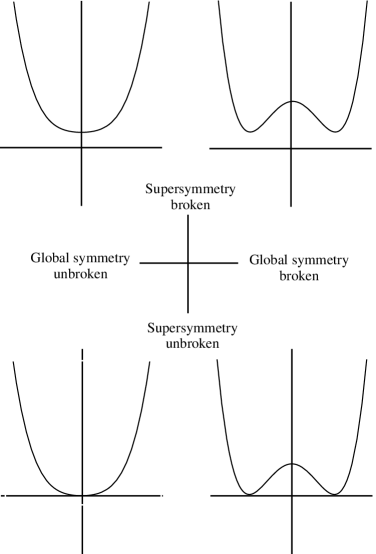
Figure 7: The vacuum energy is the order parameter for spontaneous supersymmetry
breaking.

For the case at hand, the various contributions to the scalar potential are of the following form,

$${\cal V}\ =\ {1\over 2}\,g_{1}^{2}\,D^{2}\ +\ {1\over 2}\,g_{2}^{2}\,D^{(i)2}\ +\ {1\over 2}\,g_{3}^{2}\,D^{(a)2}\ +\ |\,P_{i}\,|^{2}\ ,$$ (8.6)

If $\langle\,P_{i}\,\rangle\neq 0$ (for some $i$), $\langle\,{\cal V}\,\rangle>0$ and supersymmetry is spontaneously broken $[{\bf?}]$. On the other hand, if $\langle\,P_{i}\,\rangle=0$, a vacuum can always be found where $\langle D^{(a)}\rangle=\langle D^{(i)}\rangle=\langle D\rangle=0$, so $\langle\,{\cal V}\,\rangle=0$ and supersymmetry is preserved. Therefore the signal for spontaneous supersymmetry breaking is that $\langle\,P_{i}\,\rangle\neq 0$ for some $i$.

For the case of the MSSM, we previously found a minimum of the potential at

$$\langle\tilde{q}\rangle\;=\;\langle\tilde{l}\rangle\;=\;\langle\tilde{\bar{u}}\rangle\;=\;\langle\tilde{\bar{d}}\rangle\;=\;\langle\tilde{\bar{e}}\rangle\;=\;0$$ (8.7)

and

$$\langle h_{1}\rangle\;=\;\langle h_{2}\rangle\;=\;0\;.$$ (8.8)

Substituting these vevs into the potential, we find that the vacuum energy is zero, $\langle\,{\cal V}\,\rangle=0,$ which implies that supersymmetry is preserved.

Thus we have seen that the simplest version of the MSSM preserves supersymmetry and electroweak symmetry. Both must be broken. One way to do this is to clutter up the theory by adding more fields, which we reject out of hand. A second, more appealing approach can be found by relaxing one of the assumptions that underlie the MSSM.

In the first lecture we motivated weak-scale supersymmetry in terms of the hierarchy problem. We presented the MSSM as a fundamental theory in which the light Higgs mass was protected from destabilizing divergences. In what follows, we will keep this motivation, but discard the notion that the MSSM is a fundamental theory. Instead, we will view the MSSM as an effective theory valid below a scale $M$.

In practical terms this means that the MSSM no longer needs to be renormalizable. Indeed, it should contain an infinite tower of higher-dimensional operators suppressed by the scale $M$. The full effective theory is described by an action of the form

$$S = \int d^{4}xd^{4}\theta\;K(\Phi^{+}e^{gV},\Phi)$$ (8.9)

$$+\;\left[\,\int d^{4}xd^{2}\theta\;\bigg{(}\,{1\over 4}\,H(\Phi)\,WW\ +\ P(\Phi)\,\bigg{)}\;+\;{\rm h.c.}\,\right]$$

where $K(\Phi^{+},\Phi)$ is a real function known as the Kähler potential $[{\bf?}]$, $H(\Phi)$ is an analytic gauge potential, and $P(\Phi)$ is the analytic superpotential, each with an expansion in powers of $1/M$:

$$K(\Phi^{+},\Phi) = \Phi^{+}\Phi\;+\;\Phi^{+}\Phi\,\left({\Phi+\Phi^{+}\over M}\right)\;+\;...$$

$$H(\Phi) = 1\;+\;{1\over M}\,\Phi\;+\;...$$

$$P(\Phi) = \frac{1}{2}\,\mu\,\Phi^{2}\;+\;\frac{1}{3}\,\lambda\,\Phi^{3}\;+\;{1\over M}\,\Phi^{4}\;+\;....$$ (8.10)

The Kähler potential contains generalized kinetic terms, while the superpotential contains generalized Yukawa couplings. (In these expressions, we have not written coefficients of order one in front of the nonrenormalizable terms.)

For our purposes we do not need to know much about the theory at the scale $M$. All we need to assume is that it preserves SU(3) $\times$ SU(2) $\times$ U(1) and that it breaks supersymmetry at a scale $M_{S}$. These two facts imply that there is a chiral superfield $U$ whose $\theta\theta$ component has a vev of order $M_{S}^{2}$,

$$U\;=\;\theta\theta\;M_{S}^{2}\ .$$ (8.11)

The field $U$ is a spurion whose sole role is to communicate supersymmetry breaking to the fields of the MSSM. It contributes to the Lagrangian through nonrenormalizable terms suppressed by $1/M$, such as

$${1\over M^{2}}\int d^{4}\theta\;\Phi^{+}\Phi\;U^{+}U$$

$${1\over M}\int d^{2}\theta\;U\,W^{\alpha}W_{\alpha}$$

$${1\over M}\int d^{2}\theta\;\left[\,\frac{1}{2}\,m\,\Phi^{2}\;+\;\frac{1}{3}\,g\,\Phi^{3}\,\right]\;U\ .$$ (8.12)

For the case of the MSSM, these terms introduce a host of new parameters $[{\bf?}]$, $[{\bf?}]$:

• 5 independent $3\times 3$ mass matrices for the squarks and sleptons,

  $$M^{2}_{0i}{}^{j}\,A^{*}_{j}A^{i}\ ,$$

  as well as two independent masses for the Higgs scalars;

• 3 independent gaugino masses,

  $$M_{1/2}^{a}\,\lambda\lambda\ ,$$

  for the three factors of the standard model gauge group;

• One analytic mass for the two Higgs doublets

  $$\mu B\,h_{1}h_{2}\;;$$

• 27 analytic trilinear couplings for the scalar fields,

  $$A_{ijk}A^{i}A^{j}A^{k}\ ,$$

  where $A_{ijk}=0$ unless the coupling is allowed by gauge invariance.

For simplicity, we take the soft parameters to be real. These terms break supersymmetry explicitly in the low energy effective Lagrangian. Clearly $M_{0i}{}^{j}\simeq M_{1/2}^{a}\simeq\mu B\simeq A_{ijk}\simeq M_{W}$ for the hierarchy to be safe from destabilizing divergences.

The soft symmetry breaking operators solve several of the problems associated with the simplest version of the MSSM. For example, they lift the masses of the supersymmetric particles out of reach of present experiments. They also change the potential to permit electroweak symmetry breaking,

$$\langle h_{1}\rangle\;=\;v_{1}$$

$$\langle h_{2}\rangle\;=\;v_{2}$$ (8.13)

where $v_{1},v_{2}\neq 0$.

However, the soft supersymmetry breakings introduce their own set of problems. They enlarge the parameter space to include over 50 new parameters, so the MSSM is no longer quite so minimal. More importantly, the soft operators can induce rare processes such as flavor-changing neutral currents $[{\bf?}]$, $[{\bf?}]$. The operators must be carefully constrained.

To illustrate the problem, let us examine the canonical example of $K-\bar{K}$ mixing. We will work in a supersymmetric basis, in which the quark mass matrices are diagonal. Then the usual contributions to $K-\bar{K}$ mixing are suppressed by the GIM mechanism, as shown in Fig. 8(a).

Figure 8: Diagrams that contribute to $K-\bar{K}$ mixing. (a) The standard-model contributions are suppressed by the GIM mechanism because $VV^{\dagger}=1$. (b) The squark mass matrices give rise to supersymmetric contributions to the mixing.

In supersymmetric theories there are additional diagrams which contribute to $K-\bar{K}$ mixing. A gluino contribution is shown in Fig. 8(b). In this diagram the flavor changing neutral current (FCNC) is induced by the squark mass matrix. From the diagram one can see that the FCNC vanishes if the LL and RR entries of the squark mass matrices are proportional to the identity, and the LR entries are proportional to the Yukawa matrix, $\lambda_{D}$. Then the rotations which diagonalize the quark mass matrix,

$$u \rightarrow V_{u}\,u$$

$$d \rightarrow V_{d}\,d$$

$$\bar{u} \rightarrow V_{\bar{u}}\,\bar{u}$$

$$\bar{d} \rightarrow V_{\bar{d}}\,\bar{d}\ ,$$ (8.14)

also eliminate all terms which connect $\tilde{s}$ to $\tilde{d}$.

A second way to suppress the FCNC is to take the soft LL and RR mass matrices to be proportional to the Yukawa matrices themselves $[{\bf?}]$. Then the LL and RR terms are of the form

$$\tilde{q}^{\dagger}\,(\lambda^{*}_{U}\lambda^{T}_{U}\;+\lambda^{*}_{D}\;\lambda^{T}_{D})\;\tilde{q}$$

$$\tilde{\bar{u}}^{\dagger}\,(\lambda^{\dagger}_{U}\lambda_{U})\,\tilde{\bar{u}}$$

$$\tilde{\bar{d}}^{\dagger}\,(\lambda^{\dagger}_{D}\lambda_{D})\,\tilde{\bar{d}}\ ,$$ (8.15)

where the Yukawa couplings are matrices in flavor space. These Yukawa terms give rise to the following squark mass matrices,

$$\tilde{u}^{\dagger}\,(M_{u}^{2}\;+\;VM^{2}_{d}\;V^{\dagger})\,\tilde{u}$$

$$\tilde{d}^{\dagger}\,(M_{d}^{2}\;+\;V^{\dagger}M^{2}_{u}\;)\,\tilde{d}$$

$$\tilde{\bar{u}}^{\dagger}\,(M_{u}^{2})\,\tilde{\bar{u}}\;\;$$

$$\tilde{\bar{d}}^{\dagger}\,(M_{d}^{2})\,\tilde{\bar{d}}\ ,$$ (8.16)

where $M_{u}$ and $M_{d}$ are the diagonalized up- and down-type quark mass matrices, and $V\equiv V^{\dagger}_{u}V_{d}$ is the usual CKM matrix. For soft masses of the form (8.15), the flavor changing neutral currents are suppressed by a supersymmetric generalization of the usual GIM mechanism.

9.  Naturalness, Revisited

In the previous section we have seen that supersymmetry and gauge symmetry can be broken by operators which arise if the MSSM is an effective theory, valid below a scale $M$. In this section we will revisit the hierarchy problem to make sure that the Higgs stays light even though another scale has been introduced into the theory $[{\bf?}]$, $[{\bf?}]$. We will see whether radiative corrections still respect the electroweak hierarchy.

The subject of supersymmetric radiative corrections is rather technical, involving perturbation theory in superspace (or, involving subtle questions of regularization in components) $[{\bf?}]$. The end result is that the Kähler potential can receive perturbative radiative corrections.

$$\int d^{4}\theta\;K\ \rightarrow\ \int d^{4}\theta\;K\;+\;\int d^{4}\theta\;\delta K\;.$$ (9.1)

The superpotential, however, cannot

$$\int d^{2}\theta\;P\ \rightarrow\ \int d^{2}\theta\;P\ .$$ (9.2)

The supersymmetric nonrenormalization theorem states that the superpotential receives no corrections at all – not finite, not infinite – to any order in perturbation theory.

The standard proof of the nonrenormalization theorem requires superfield perturbation theory, which is too technical for these lectures. Instead, let us prove the theorem in a manner discussed by Seiberg $[{\bf?}]$. Consider the Lagrangian

$$\int d^{4}\theta\;\Phi^{+}_{i}\Phi^{i}\ +\ \;\Big{[}\int d^{2}\theta\,\Big{(}\,{1\over 2}\,m_{ij}\,\Phi^{i}\Phi^{j}\;+\;{1\over 3}\,\lambda_{ijk}\,\Phi^{i}\Phi^{j}\Phi^{k}\,\Big{)}\;+\;{\rm h.c.}\Big{]}\;.$$ (9.3)

In what follows, we will think of $m_{ij}$ and $\lambda_{ijk}$ as the vev’s of classical background superfields. In other words, we will take their kinetic energies to be

$$\lim_{\Lambda\rightarrow\infty}\;\Lambda^{2}\;\int d^{4}\theta\;(m^{ij+}m_{ij}\;+\;\lambda^{ijk+}\lambda_{ijk})\;,$$ (9.4)

in which case the fields have dimension zero and do not propagate.

The action (9.3) is manifestly invariant under a global U(N) symmetry. It is also invariant under a continuous $R$-symmetry, with $R$-charges assigned as follows:

$$\theta \rightarrow e^{-i\alpha}\;\theta$$

$$\Phi^{i} \rightarrow e^{i\alpha}\;\Phi^{i}$$

$$m_{ij} \rightarrow m_{ij}$$

$$\lambda_{ijk} \rightarrow e^{-i\alpha}\;\lambda_{ijk}\;.$$ (9.5)

The U(N) $\times$ U(1)_R symmetry plays a major role in constraining the quantum corrections.

As a first step towards proving the theorem, we consider the renormalization of the $\Phi^{3}$ term in the superpotential. At one loop, the correction cannot involve $\lambda^{+}$ or $m^{+}$ because the superpotential must be analytic. Therefore the only U(N) invariant is of the form

$$\lambda_{...}\lambda_{...}\lambda_{...}\;m^{-1..}m^{-1..}\;\Phi^{.}\Phi^{.}\Phi^{.}\;,$$ (9.6)

where the dots denote U(N) indices contracted in different ways. The problem with this term is that it violates $R$-symmetry. More insertions of $\lambda$ makes this even worse, so there can be no renormalization of the $\Phi^{3}$ coupling. (Nonperturbative corrections of the form $\exp(-m/\lambda\Phi)$ are not permitted because they are singular at weak coupling for negative $\Phi$.)

Now let us consider a higher-dimensional operator, such as a possible $\Phi^{5}$ coupling. A contribution of the form

$$\lambda_{...}\lambda_{...}\lambda_{...}\;m^{-1..}m^{-1..}\;\Phi^{.}\Phi^{.}\Phi^{.}\Phi^{.}\Phi^{.}\;$$ (9.7)

is U(N) $\times$ U(1)_R invariant. However, this term corresponds to the diagram of Fig. 9. This diagram is not 1PI, so it does not correspond to a term in the renormalized superpotential.

Figure 9: This $\Phi^{5}$ diagram is not 1PI and does not contribute to the renormalized
superpotential.

These arguments can be readily extended to all other operators. For the case at hand, the superpotential is not renormalized, either perturbatively or

nonperturbatively, because of

1. analyticity,

2. global U(N) symmetry,

3. global U(1)_R symmetry, and

4. a smooth weak-coupling limit.

Let us now apply the nonrenormalization theorem to the study of naturalness in supersymmetric theories. The theorem tells us that all potentially destabilizing renormalizations are corrections to the Kähler potential. To classify the dangerous diagrams, we need to determine the superspace degree of divergence.

Superspace power counting is not hard to derive. A diagram with $E_{\Phi}$ external chiral superfields has the following cutoff dependence,

$$\Lambda^{D}\;\int d^{4}\theta\;\Phi^{+}\;...\;\Phi\;,$$ (9.8)

where $D\leq 2-E_{\Phi}+\sum dV_{d}$, and $V_{d}$ denotes the number of nonrenormalizable operators suppressed by $(1/M)^{d}$. If we include the factors of $1/M$, we see that the divergence associated with a given diagram goes like

$$\Lambda^{D}\;\prod_{d}\,\left({1\over M}\right)^{dV_{d}}\;\mathrel{\mathchoice{\vbox{\offinterlineskip\halign{$\m@th\displaystyle\hfil#\hfil$\cr<\crcr\sim\crcr} }}{\vbox{\offinterlineskip\halign{$\m@th\textstyle\hfil#\hfil$\cr<\crcr\sim\crcr} }}{\vbox{\offinterlineskip\halign{$\m@th\scriptstyle\hfil#\hfil$\cr<\crcr\sim\crcr} }}{\vbox{\offinterlineskip\halign{$\m@th\scriptscriptstyle\hfil#\hfil$\cr<\crcr\sim\crcr} }}}\;M^{2-E_{\Phi}}\ ,$$ (9.9)

for $\Lambda\mathrel{\mathchoice{\vbox{\offinterlineskip\halign{$\m@th\displaystyle\hfil#\hfil$\cr<\crcr\sim\crcr} }}{\vbox{\offinterlineskip\halign{$\m@th\textstyle\hfil#\hfil$\cr<\crcr\sim\crcr} }}{\vbox{\offinterlineskip\halign{$\m@th\scriptstyle\hfil#\hfil$\cr<\crcr\sim\crcr} }}{\vbox{\offinterlineskip\halign{$\m@th\scriptscriptstyle\hfil#\hfil$\cr<\crcr\sim\crcr} }}}M$. Superspace power counting indicates that the only dangerous diagrams are tadpoles, with $E_{\Phi}=1$.

To see why tadpoles are dangerous, let us consider a specific example in which we restrict our attention to a single “Higgs” superfield, $H$. We will let $N$ be a gauge- and global-symmetry singlet chiral superfield which couples directly to the Higgs. Therefore we will take the superpotential, $P$, to be

$$P\;=\;{1\over 2}\,\mu\,H^{2}\;+\;{1\over 2}\,m\,N^{2}\;+\;\lambda\,NH^{2}\;+\;...,$$ (9.10)

where we fix the Higgs mass $M_{h}=\mu\simeq m\simeq M_{W}$. (A discrete $Z_{2}$ symmetry replaces the gauge symmetry of the standard model. We assume that $Z_{2}$ is not broken for scales larger than $M_{W}$.) The hierarchy is destabilized if radiative corrections lift $M_{h}\gg M_{W}$.

Now let us suppose that our theory is a low energy effective theory, coupled by nonrenormalizable operators to the spurion $U$. In this case, the Kähler potential becomes

$$K\;=\;\bigg{[}\,N^{+}N\;+\;H^{+}H\;+\;H^{+}H\,\bigg{(}{N+N^{+}\over M}\bigg{)}\,\bigg{]}\bigg{\{}\,1\;+\;\bigg{(}{U+U^{+}\over M}\bigg{)}\;+\;...\,\bigg{\}}$$ (9.11)

where we have neglected coefficients of order one. Typically, the fields $H$ and $N$ have weak-scale vevs,

$$\langle H\rangle \mathrel{\mathchoice{\vbox{\offinterlineskip\halign{$\m@th\displaystyle\hfil#\hfil$\cr<\crcr\sim\crcr} }}{\vbox{\offinterlineskip\halign{$\m@th\textstyle\hfil#\hfil$\cr<\crcr\sim\crcr} }}{\vbox{\offinterlineskip\halign{$\m@th\scriptstyle\hfil#\hfil$\cr<\crcr\sim\crcr} }}{\vbox{\offinterlineskip\halign{$\m@th\scriptscriptstyle\hfil#\hfil$\cr<\crcr\sim\crcr} }}} M_{W}\;+\;\theta\theta M_{W}^{2}$$ (9.20)

$$\langle N\rangle \mathrel{\mathchoice{\vbox{\offinterlineskip\halign{$\m@th\displaystyle\hfil#\hfil$\cr<\crcr\sim\crcr} }}{\vbox{\offinterlineskip\halign{$\m@th\textstyle\hfil#\hfil$\cr<\crcr\sim\crcr} }}{\vbox{\offinterlineskip\halign{$\m@th\scriptstyle\hfil#\hfil$\cr<\crcr\sim\crcr} }}{\vbox{\offinterlineskip\halign{$\m@th\scriptscriptstyle\hfil#\hfil$\cr<\crcr\sim\crcr} }}} M_{W}\;+\;\theta\theta M_{W}^{2}\;,$$ (9.29)

while

$$\langle U\rangle\;\simeq\;\theta\theta M_{S}^{2}\;.$$ (9.30)

The vevs (9.29) and (9.30) preserve hierarchy, as can be seen by substituting into (9.10) and (9.11). They induce a supersymmetry-breaking mass of order $M_{W}$ for the scalar component of the Higgs superfield.

Figure 10: Potentially dangerous tadpole diagrams.

At one loop, these vevs can shift. In the above example, there are two potentially dangerous superspace diagrams, as shown in Fig. 10. Each $U^{+}$ insertion induces a quadratic divergence

$$\delta S\ \simeq\ {\Lambda^{2}\over M^{2}}\,\int d^{4}xd^{4}\theta\;U^{+}N\;+\;....$$ (9.31)

Taking the cutoff $\Lambda\simeq M$, we find

$$\delta S \simeq \int d^{4}xd^{4}\theta\;U^{+}N\;+\;...$$ (9.32)

$$\simeq M^{2}_{S}\int d^{4}xd^{2}\theta\;N\;+\;....$$

This term induces a vev of order $M^{2}_{S}$ for $F_{N}$, which in turn gives rise to masses of order $M_{S}$ for the scalar fields $n$ and $h$. The hierarchy is, in fact, destabilized.

This example illustrates that the hierarchy can be destabilized when a second scale is introduced into the theory. However, the destabilization requires a gauge- and global-symmetry singlet, so the MSSM is safe. The next-to-minimal standard model is not necessarily safe because it contains a singlet superfield, $N$.

Even for the MSSM, however, the quadratically divergent radiative corrections carry an important lesson: the soft supersymmetry-breaking parameters cannot be calculated in terms of the low-energy effective field theory. They depend sensitively on physics at the scale $M$. This can be seen by considering the following terms in the Kähler potential,

$${1\over M}\,\bigg{[}\,\lambda_{U}\,Q\bar{U}H^{+}_{1}\;+\;\lambda_{D}\,Q\bar{D}H^{+}_{2}\,\bigg{]}\ \bigg{\{}\,1\;+\;\bigg{(}{U+U^{+}\over M}\bigg{)}\,\bigg{\}}\;.$$ (9.33)

These terms give rise to quadratically divergent diagrams such as those in Fig. 11. When reduced to components, they give rise to additive renormalizations of the squark masses, such as

$$M^{4}_{S}\,\left({\Lambda^{2}\over M^{4}}\right)\,\tilde{\bar{u}}^{\dagger}\,(\lambda^{\dagger}_{U}\lambda_{U})\,\tilde{\bar{u}}\;.$$ (9.34)

This operator has the same flavor structure as in eq. (8.15). For $\Lambda\mathrel{\mathchoice{\vbox{\offinterlineskip\halign{$\m@th\displaystyle\hfil#\hfil$\cr<\crcr\sim\crcr} }}{\vbox{\offinterlineskip\halign{$\m@th\textstyle\hfil#\hfil$\cr<\crcr\sim\crcr} }}{\vbox{\offinterlineskip\halign{$\m@th\scriptstyle\hfil#\hfil$\cr<\crcr\sim\crcr} }}{\vbox{\offinterlineskip\halign{$\m@th\scriptscriptstyle\hfil#\hfil$\cr<\crcr\sim\crcr} }}}M$, it does not destroy the hierarchy. However, the quadratic divergence tells us that the coefficients of the soft supersymmetry breaking operators cannot be calculated in terms of the low energy effective theory. They depend on physics at the scale $M$, and must be fixed by matching conditions at that scale $[{\bf?}]$.

Figure 11: A quadratically divergent renormalization of the soft squark mass.

10.  Electroweak Symmetry Breaking

In the previous section we have seen that the MSSM with arbitrary soft supersymmetry breaking contains over 50 new parameters. Indeed, it may well be that nature adjusts each of them independently to describe the physical world. However, as a first step towards understanding the phenomenology of supersymmetric models, it makes sense to shrink the parameter space to a more manageable size.

Figure 12: In supersymmetric theories, the running gauge couplings unify at the scale $M_{\rm GUT}\simeq 10^{16}$ GeV.

Since the soft symmetry breakings originate at the scale $M$, restrictions on the parameters amount to assumptions about physics at that scale $[{\bf?}]$, $[{\bf?}]$. Therefore in what follows we will be motivated by the fact that – in supersymmetric theories – the running gauge couplings unify at a scale $M_{\rm GUT}\simeq 10^{16}$ GeV $[{\bf?}]$, $[{\bf?}]$, $[{\bf?}]$, $[{\bf?}]$, as shown in Fig. 12. In light of this, it is reasonable to assume that the soft parameters unify as well, in which case they are completely specified by four parameters at the scale $M_{\rm GUT}$,

1. One common scalar mass, $M_{0}$;

2. One common gaugino mass, $M_{1/2}$;

3. One analytic Higgs mass, $B\mu$;

4. One trilinear coupling, $A_{0}\,\lambda_{F}$;

where $A_{0}$ is the soft parameter and $\lambda_{F}$ is the appropriate Yukawa coupling from the superpotential.

Of course, experimental physics is done at the weak scale, so these parameters must be evolved to $M_{W}$ using the renormalization group equations $[{\bf?}]$. This is fortunate because – if the scalar masses, $M_{0}$, were degenerate at the weak scale – either no gauge symmetries would be broken, or all would be broken.

Thus, at the weak scale, the effective potential is of the form

$${\cal V} = \ {1\over 2}\,g_{1}^{2}\,D^{2}\;+\;{1\over 2}\,g_{2}^{2}\,D^{(i)2}\;+\;{1\over 2}\,g_{3}^{2}\,D^{(a)2}\;+\;|\,P_{i}\,|^{2}\;$$ (10.1)

$$+\;M^{2}_{Q}\,\tilde{q}^{\dagger}\tilde{q}\;+\;M^{2}_{\bar{U}}\,\tilde{\bar{u}}^{\dagger}\tilde{\bar{u}}\;+\;M^{2}_{\bar{D}}\,\tilde{\bar{d}}^{\dagger}\tilde{\bar{d}}$$

$$+\;M^{2}_{L}\,\tilde{l}^{\dagger}\tilde{l}\;+\;M^{2}_{\bar{E}}\,\tilde{\bar{e}}^{\dagger}\tilde{\bar{e}}\;+\;M^{2}_{1}\,h_{1}^{\dagger}h_{1}\;+\;M^{2}_{2}\,h_{2}^{\dagger}h_{2}$$

$$+\;\bigg{\{}\,\bigg{[}A^{U}_{ij}\,\tilde{q}^{i}\tilde{\bar{u}}^{\,j}h_{2}\;+\;A^{D}_{ij}\,\tilde{q}^{i}\tilde{\bar{d}}^{\,j}h_{1}\;+\;A^{E}_{ij}\,\tilde{l}^{i}\tilde{\bar{e}}^{\,j}h_{1}$$

$$+\;\mu\,B\,h_{1}h_{2}\,\bigg{]}\;+\;{\rm h.c.}\;\bigg{\}}\ ,$$

where, at the unification scale, we impose the boundary condition

$$M^{2}_{Q}\ =\ M^{2}_{\bar{U}}\ =\ M^{2}_{\bar{D}}\ =\ M^{2}_{L} = M^{2}_{\bar{E}}\ =\ M^{2}_{1}\ =\ M^{2}_{2}\ \equiv\ M^{2}_{0}$$

$$A^{U}_{ij}\ \equiv\ \lambda_{Uij}\,A_{0}\qquad A^{D}_{ij} \equiv \lambda_{Dij}\,A_{0}\ \qquad A^{E}_{ij}\ \equiv\ \lambda_{Eij}\,A_{0}$$

$$B\mu \equiv B\mu\ .$$ (10.2)

The full computation of the effective potential is beyond the scope of these lectures. To grasp the idea, however, we will focus on the most important corrections to the soft scalar masses. For this purpose, it is sufficient to consider the effects of the top Yukawa $\lambda_{T}$. (The strong gauge coupling does not contribute to the running of the squark masses at one loop.)

Figure 13: Diagrams that contribute to the running of the soft squark masses. Each diagram requires insertions of the spurions $U$ and $U^{+}$ on its lines and vertices.

The top Yukawa $\lambda_{T}$ links the fields $H_{2}$, $T$ and $\bar{T}$ in the superpotential. These couplings renormalize the mass parameters $M^{2}_{2}$, $M^{2}_{T}$ and $M^{2}_{\bar{T}}$ through diagrams like those of Fig. 13. The resulting renormalization group equations are $[{\bf?},{\bf?}]$

$$Q\,{d\over dQ}\,\pmatrix{M^{2}_{2}\crcr\vskip 3.0pt\cr M^{2}_{\bar{T}}\crcr\vskip 3.0pt\cr M^{2}_{T}\crcr\vskip 3.0pt\cr}\;=\;{\lambda^{2}_{T}\over 8\pi^{2}}\,\pmatrix{3&3&3\crcr\vskip 3.0pt\cr 2&2&2\crcr\vskip 3.0pt\cr 1&1&1\crcr\vskip 3.0pt\cr}\pmatrix{M^{2}_{2}\crcr\vskip 3.0pt\cr M^{2}_{\bar{T}}\crcr\vskip 3.0pt\cr M^{2}_{T}\crcr\vskip 3.0pt\cr}\;+\;{\lambda^{2}_{T}\over 8\pi^{2}}\,|\,A^{T}\,|^{2}\,\pmatrix{3\crcr\vskip 3.0pt\cr 2\crcr\vskip 3.0pt\cr 1\crcr\vskip 3.0pt\cr}\;,$$ (10.3)

where the factors of three come from the three colors running around the loop of Fig. 13. Likewise, the factors of two come from SU(2). (The color coupling does not contribute to the renormalization group equations at this order.)

Figure 14: A sample spectrum in the radiative breaking scenario. Here $M_{0}=300$ GeV and $M_{1/2}=100$ GeV. The solid lines denote squark masses and the dotted lines sleptons. (The lightest squark is predominantly $\bar{t}$.) The dashed lines represent gaugino masses, while the dot-dashed line marks the mass of the second Higgs.

To analyze this equation, let us forget that $\lambda_{T}$ runs, and also ignore the term with $A^{T}$, for simplicity. Then the evolution of the masses is determined by the matrix

$$\pmatrix{3&3&3\cr 2&2&2\cr 1&1&1\cr}\;.$$ (10.4)

This matrix has eigenvalues $(0,0,6)$. At the Planck scale, the initial condition on the soft masses can be written in terms of the eigenvectors,

$$\pmatrix{M^{2}_{2}\crcr\vskip 3.0pt\cr M^{2}_{\bar{T}}\crcr\vskip 3.0pt\cr M^{2}_{T}\crcr\vskip 3.0pt\cr} = \;M^{2}_{0}\,\pmatrix{1\crcr\vskip 3.0pt\cr 1\crcr\vskip 3.0pt\cr 1\crcr\vskip 3.0pt\cr}$$ (10.5)

$$= \;{1\over 2}\,M^{2}_{0}\,\left[\pmatrix{0\crcr\vskip 3.0pt\cr-1\crcr\vskip 3.0pt\cr 1\crcr\vskip 3.0pt\cr}\right.\ +\ \pmatrix{-1\crcr\vskip 3.0pt\cr 1\crcr\vskip 3.0pt\cr 0\crcr\vskip 3.0pt\cr}\ +\ \left.\pmatrix{3\crcr\vskip 3.0pt\cr 2\crcr\vskip 3.0pt\cr 1\crcr\vskip 3.0pt\cr}\right]\;.$$

The last eigenvector corresponds to the eigenvalue $6$, so it is damped out during the renormalization from $M$ to $M_{W}$. The other eigenvectors have eigenvalues zero, so they barely run. Therefore, at $M_{W}$, we expect to find

$$\pmatrix{M^{2}_{2}\crcr\vskip 3.0pt\cr M^{2}_{\bar{T}}\crcr\vskip 3.0pt\cr M^{2}_{T}\crcr\vskip 3.0pt\cr}\;\simeq\;{1\over 2}\,M^{2}_{0}\,\pmatrix{-1\crcr\vskip 3.0pt\cr 0\crcr\vskip 3.0pt\cr 1\crcr\vskip 3.0pt\cr}\;.$$ (10.6)

We see that the renormalization group evolution has flipped the sign of the $h_{2}$ mass term. The large top Yukawa has destabilized the vacuum: the effective potential breaks SU(2) $\times$ U(1) down to the U(1) of electromagnetism!

The effect of the renormalization group evolution on the supersymmetric mass spectrum is shown in Fig. 14, where we plot some of the running supersymmetric masses between the weak and unification scales. Indeed, as expected, the mass (squared) of the second Higgs is driven negative, and the right-handed top squark is lighter than the others.

Figure 15: The mass of the lightest supersymmetric particle, $\chi^{0}_{1}$, for $\mu>0$, $A_{0}=0$, $\alpha_{s}(M_{Z})=0.12$ and $m_{t}=175$ GeV. The shaded region is forbidden by experimental and theoretical constraints. Most of the supersymmetric parameter space is still open.

Thus we have seen that in this theory, electroweak symmetry breaking is driven by a generalization of the Coleman-Weinberg mechanism $[{\bf?}]$, where the large radiative corrections are induced by the top mass. This mechanism requires $M_{t}\simeq 175$ GeV. This remarkable fact links electroweak symmetry breaking to the presence of a heavy top! 

11.  Experimental Expectations

In what follows, we present expectations for the supersymmetric spectrum based on this unification scenario. (For more details, see the lectures of Tata $[{\bf?}]$.) Since electroweak symmetry is broken, we shall trade the parameters $g_{1},\;g_{2},\;\mu$ and $B\mu$ for the mass of the $Z$, $M_{Z}$, the Fermi coupling, $G_{F}$, the fine structure constant, $\alpha_{EM}$, and the ratio of vevs, $\tan\beta=v_{2}/v_{1}$. We take the strong coupling, $\alpha_{s}$, and the ordinary fermion masses to be given by their experimental values.

Figure 16: The mass of the up squark (solid line) and the gluino (dashed line), for $\mu>0$, $A_{0}=0$, $\alpha_{s}(M_{Z})=0.12$ and $M_{t}=175$ GeV. The parameter space corresponds to squark masses of less than about one TeV.

In this way we can compute the supersymmetric masses and couplings in terms of the parameters

$$M_{0}\qquad M_{1/2}\qquad A_{0}\qquad\tan\beta$$ (11.1)

and the sign of $\mu$. For simplicity, we shall set $A_{0}=0$ and take the supersymmetric Higgs mass parameter $\mu>0$.

In Fig. 15 we show mass contours for the lightest superparticle, $\chi^{0}_{1}$. The $\chi^{0}_{1}$ is neutral and stable (because of R-parity). In the figure, the shaded areas represent forbidden regions of parameter space, either because of present experimental limits or because of theoretical constraints such as the cosmological requirement that the lightest (stable) superparticle be neutral, or the phenomenological constraint that electroweak symmetry be broken, but not color.

In Fig. 16 we show contours for the (up) squark and the gluino masses. (The masses of the up, down, charm and strange squarks are almost degenerate.) From the plot we see that the parameter space covers squark masses up to about 1 TeV. This is the range of interest if supersymmetry is to solve the hierarchy problem. (The rule of thumb is that $M_{\tilde{g}}\simeq 3M_{1/2}$ and $M^{2}_{\tilde{q}}\simeq M^{2}_{0}+4M^{2}_{1/2}$.)

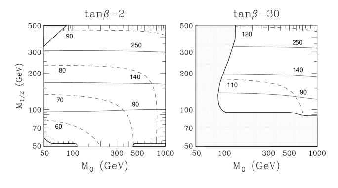
Figure 17: The mass of the lightest chargino, $\chi^{\pm}_{1}$, (solid line) and lightest Higgs, $h$, (dashed line), for $\mu>0$, $A_{0}=0$, $\alpha_{s}(M_{Z})=0.12$ and $M_{t}=175$ GeV. The Higgs mass is less than about 120 GeV over the parameter space.

In Fig. 17 we plot contours for the masses of the lightest Higgs scalar, $h$, and the lightest chargino, $\chi^{\pm}_{1}$. We see that $M_{\chi^{\pm}}\simeq M_{1/2}$, and that the maximum Higgs mass is about 120 GeV. (For completeness, we note that the slepton masses are approximately $M_{L}\simeq M_{0}$.)

Figure 18: The mass of the charged Higgs, $H^{\pm}$, (solid line) and lightest top squark, $\tilde{t}_{1}$, (dashed line), for $\mu>0$, $A_{0}=0$, $\alpha_{s}(M_{Z})=0.12$ and $M_{t}=175$ GeV. The decays $t\rightarrow\tilde{t}\tilde{\chi}^{0}_{1}$ and $t\rightarrow H^{+}b$ are kinematically forbidden over most of the parameter space.

Finally, in Fig. 18 we show contours for the masses of the lightest top squark, $\tilde{t}_{1}$, and charged Higgs, $H^{\pm}$. From the figure we see that the decays $t\rightarrow\tilde{t}_{1}\tilde{\chi}^{0}_{1}$ and $t\rightarrow H^{+}b$ are kinematically forbidden over most of the parameter space. (The top squark can be lighter for $A_{0}\neq 0$, but a very light stop requires a fine tuning of the parameters.)

These figures can be used to illustrate the supersymmetry reach of a given accelerator. For example, LEP 200 has a mass reach of about $\sqrt{s}-100$ GeV for a supersymmetric Higgs particle, and $\sqrt{s}/2$ for a chargino $[{\bf?}]$. (Sample processes are illustrated in Fig. 19.) Therefore Fig. 17 shows that LEP 200 has an excellent chance of discovering the lightest supersymmetric Higgs, and a reasonable possibility of finding the lightest chargino.

Figure 19: Sample processes contributing to (a) Higgs, and (b) chargino, discovery
at LEP 200.

The Tevatron’s discovery potential is more model-dependent, and varies considerably with the Tevatron luminosity. For an integrated luminosity between 200 pb^-1 and 25 fb^-1, the gluino discovery reach is in the range of 300 – 400 GeV. Likewise, the chargino/neutralino reach varies between 150 – 250 GeV in the trilepton decay channel, $\chi^{+}_{1}\chi^{0}_{2}\rightarrow\ell^{+}\ell^{-}\ell^{\prime+}$ plus missing energy $[{\bf?}]$. (Sample processes are illustrated in Fig. 20.) From Figs. 16 and 17 we see that an upgraded Tevatron would begin to cover a significant amount of the supersymmetric parameter space.

Finally, the LHC has an immense discovery potential. Assuming 10 fb^-1 of luminosity, recent studies indicate that the LHC’s reach for gluinos extends significantly past 1 TeV $[{\bf?}]$. There are promising signals in the jets plus missing energy channel, as well as in channels with leptons and missing energy. Clearly, understanding LHC signals and backgrounds is of enormous importance for supersymmetry. The great energy of LHC collisions offers unparalleled opportunities for supersymmetry discovery.

12.  Conclusions

These lectures presented an introduction to the theory and practice of weak-scale supersymmetry. We motivated the subject in terms of the hierarchy problem, the instability of the Higgs mass to quadratically divergent radiative corrections. We found that supersymmetry renders the Higgs mass natural, and gives rise to a rich new spectroscopy at the TeV scale. For every particle of the standard model, supersymmetry predicts another that has yet to be observed.

Exact supersymmetry implies Bose-Fermi mass degeneracy, so the question of supersymmetry breaking is of paramount importance for supersymmetric theories. During the course of the lectures we found that the soft supersymmetry breakings lift the masses of the supersymmetric particles into a phenomenologically acceptable range. Soft supersymmetry breaking suggests that we think of the supersymmetric standard model as an effective field theory, valid below some scale, $M$. From this point of view, supersymmetry breaking occurs at the scale $M$, and gives rise to soft operators at the scale $M_{W}$.

With LEP 200, the Fermilab Main Injector and the LHC, prospects look bright for future experiments. These accelerators will, for the first time, begin to probe large regions of the supersymmetric parameter space. Ultimately, experiments must say whether supersymmetry is correct. If it is, theorists and experimentalists must search for clues to the origin of supersymmetry breaking – the central question behind the MSSM.

Appendix

In this Appendix I will give a brief review of two-component spinor notation $[{\bf?}]$. Two-component spinors provide the most natural spinor representations of the Lorentz group in theories with chiral fermions, such as the standard model or supersymmetry. The notation exploits the fact that spinor representations of the Lorentz group are actually two-dimensional representations of its universal covering group, SL(2,$C$).

To begin, let us define $M$ to be a two-by-two matrix of determinant one: $M\in$ SL(2,$C$). The matrix $M$, its complex conjugate $M^{*}$, its transpose inverse $(M^{T})^{-1}$, and its hermitian conjugate inverse $(M^{\dagger})^{-1}$ are all representations of SL(2,$C$). These matrices represent the action of the Lorentz group on two-component Weyl spinors.

Two-component spinors with upper or lower dotted or undotted indices are defined to transform as follows under SL(2,$C$):

$$\psi^{\prime}_{\alpha}\;=\;M_{\alpha}{}^{\beta}\,\psi_{\beta} \bar{\psi}^{\prime}_{\dot{\alpha}}\;=\;M^{*}{}_{\dot{\alpha}}{}^{\dot{\beta}}\,\bar{\psi}_{\dot{\beta}}$$

$$\psi^{\prime\alpha}\;=\;M^{-1}{}_{\beta}{}^{\alpha}\,\psi^{\beta} \bar{\psi}^{\prime{\dot{\alpha}}}\;=\;(M^{*}){}^{-1}{}_{{\dot{\beta}}}{}^{{\dot{\alpha}}}\,\bar{\psi}^{\dot{\beta}}.$$ (A.1)

The spinors are denoted by Greek indices. Those with dotted indices transform in the $(0,{1\over 2})$ representation of the Lorentz group, while those with undotted indices transform in the $({1\over 2},0)$ conjugate representation.

The map from SL(2,$C$) to the Lorentz group is established through the $\sigma$-matrices,

$$\begin{array}[]{rclcrcl}\sigma^{0}&=&\pmatrix{-1&0\cr 0&-1\cr}&&\sigma^{1}&=&\pmatrix{0&1\cr 1&0\cr}\\[17.07164pt] \sigma^{2}&=&\pmatrix{0&-i\cr i&0\cr}&&\sigma^{3}&=&\pmatrix{1&0\cr 0&-1\cr}\;,\end{array}$$ (A.2)

The $\sigma$ matrices form a basis for two-by-two complex matrices,

$$P\;\equiv\;(p_{m}\sigma^{m})\;=\;\pmatrix{-p_{0}+p_{3}&p_{1}-ip_{2}\cr p_{1}+ip_{2}&-p_{0}-p_{3}\cr}\;.$$ (A.3)

Any hermitian matrix may be expanded with the $p_{m}$ real.

From any hermitian matrix $P$, we may always obtain another by the following transformation,

$$P^{\prime}\;=\;MPM^{\dagger}\;.\$$ (A.4)

Both $P$ and $P^{\prime}$ have expansions in $\sigma$,

$$(\sigma^{m}p^{\prime}_{m})\;=\;M\,(\sigma^{m}p_{m})\,M^{\dagger}\;,\$$ (A.5)

with $p_{m}$ and $p^{\prime}_{m}$ real. Since $M$ is unimodular (det $M$ = 1), the coefficients $p_{m}$ and $p^{\prime}_{m}$ are related by a Lorentz transformation:

$${\rm det}(\sigma^{m}p^{\prime}_{m})\;=\;{\rm det}(\sigma^{m}p_{m})\;=\;p_{0}^{\,\prime\,2}\;-\;{\vec{p}}^{\;\prime\,2}\;=\;p_{0}^{2}\;-\;{\vec{p}}^{\;2}\;.\$$ (A.6)

Vectors and tensors are distinguished from spinors by their Latin indices.

From (A.1) and (A.5), we see that $\sigma^{m}$ has the following index structure:

$$\sigma^{m}_{\alpha{\dot{\alpha}}}\;.\$$ (A.7)

With these conventions, $\psi^{\alpha}\psi_{\alpha}$, $\bar{\psi}_{\dot{\alpha}}\bar{\psi}^{\dot{\alpha}}$ and $\psi^{\alpha}\sigma_{\alpha{\dot{\alpha}}}^{m}\partial_{m}\bar{\psi}^{\dot{\alpha}}$ are all Lorentz scalars.

Because $M$ is unimodular, the antisymmetric tensors $\epsilon^{\alpha\beta}$ and $\epsilon_{\alpha\beta}$ $(\epsilon_{21}=\epsilon^{12}=1,\epsilon_{12}=\epsilon^{21}=-1,\epsilon_{11}=\epsilon_{22}=0)$ are invariant under Lorentz transformations,

$$\epsilon_{\alpha\beta} = M_{\alpha}{}^{\gamma}M_{\beta}{}^{\delta}\epsilon_{\gamma\delta}$$

$$\epsilon^{\alpha\beta} = \epsilon^{\gamma\delta}M_{\gamma}{}^{\alpha}M_{\delta}{}^{\beta}\;.$$ (A.8)

This implies that spinors with upper and lower indices are related through the$\epsilon$-tensor,

$$\psi^{\alpha}\;=\;\epsilon^{\alpha\beta}\,\psi_{\beta},\qquad\psi_{\alpha}\;=\;\epsilon_{\alpha\beta}\,\psi^{\beta}\;.$$ (A.9)

Note that we have defined $\epsilon_{\alpha\beta}$ and $\epsilon^{\alpha\beta}$ such that $\epsilon_{\alpha\beta}\epsilon^{\beta\gamma}=\delta_{\alpha}{}^{\gamma}$. Analogous statements hold for the $\epsilon$-tensor with dotted indices.

The $\epsilon$-tensor may also be used to raise the indices of the $\sigma$-matrices,

$$\bar{\sigma}^{m{\dot{\alpha}}\alpha}\;=\;\epsilon^{{\dot{\alpha}}{\dot{\beta}}}\epsilon^{\alpha\beta}\,\sigma^{m}_{\beta{\dot{\beta}}}\;.$$ (A.10)

From the definition of the $\sigma$-matrices, we find

$$(\sigma^{m}\bar{\sigma}^{n}+\sigma^{n}\bar{\sigma}^{m})_{\alpha}{}^{\beta} = -\;2\,g^{mn}\delta_{\alpha}{}^{\beta}$$

$$(\bar{\sigma}^{m}\sigma^{n}+\bar{\sigma}^{n}\sigma^{m})^{{\dot{\alpha}}}{}_{\dot{\beta}} = -\;2\,g^{mn}\delta^{\dot{\alpha}}{}_{\dot{\beta}}\;,$$ (A.11)

and

$${\rm Tr}\,\sigma^{m}\bar{\sigma}^{n} = -\;2\,g^{mn}$$

$$\sigma_{\alpha{\dot{\alpha}}}^{m}\bar{\sigma}_{m}{}^{{\dot{\beta}}\beta} = -\;2\,\delta_{\alpha}{}^{\beta}\delta_{\dot{\alpha}}{}^{\dot{\beta}}\;,$$ (A.12)

where $g_{mn}={\rm diag}(-1,1,1,1)$. These relations may be used to convert a vector to a bispinor and vice versa:

$$v_{\alpha{\dot{\alpha}}}\;=\;\sigma_{\alpha{\dot{\alpha}}}^{m}\,v_{m}\;,\qquad v^{m}=-\;{1\over 2}\;\bar{\sigma}^{m{\dot{\alpha}}\alpha}\,v_{\alpha{\dot{\alpha}}}\;.$$ (A.13)

The generators of the Lorentz group in the spinor representation are given by

$$\sigma^{nm}{}_{\alpha}{}^{\beta} = {1\over 4}\,(\sigma_{\alpha{\dot{\alpha}}}^{n}\bar{\sigma}^{m{\dot{\alpha}}\beta}-\sigma_{\alpha{\dot{\alpha}}}^{m}\bar{\sigma}^{n{\dot{\alpha}}\beta})$$

$$\bar{\sigma}^{nm{\dot{\alpha}}}{}_{\dot{\beta}} = {1\over 4}\,(\bar{\sigma}^{n{\dot{\alpha}}\alpha}\sigma_{\alpha{\dot{\beta}}}^{m}-\bar{\sigma}^{m{\dot{\alpha}}\alpha}\sigma_{\alpha{\dot{\beta}}}^{n})\;.$$ (A.14)

Other useful relations involving the $\sigma$-matrices are

$$\bar{\sigma}^{a}\sigma^{b}\bar{\sigma}^{c}\;-\;\bar{\sigma}^{c}\sigma^{b}\bar{\sigma}^{a} = -2i\,\epsilon^{abcd}\bar{\sigma}_{d}$$

$$\sigma^{a}\bar{\sigma}^{b}\sigma^{c}\;-\;\sigma^{c}\bar{\sigma}^{b}\sigma^{a} = 2i\epsilon^{abcd}\sigma_{d}\;,$$ (A.15)

where $\epsilon_{0123}=-1$, as well as

$$\sigma^{a}\bar{\sigma}^{b}\sigma^{c}\;+\;\sigma^{c}\bar{\sigma}^{b}\sigma^{a} = 2(g^{ac}\sigma^{b}\;-\;g^{bc}\sigma^{a}\;-\;g^{ab}\sigma^{c})$$

$$\bar{\sigma}^{a}\sigma^{b}\bar{\sigma}^{c}\;+\;\bar{\sigma}^{c}\sigma^{b}\bar{\sigma}^{a} = 2(g^{ac}\bar{\sigma}^{b}\;-\;g^{bc}\bar{\sigma}^{a}\;-\;g^{ab}\bar{\sigma}^{c})$$ (A.16)

and

$$\sigma_{\alpha{\dot{\alpha}}}^{n}\sigma_{\beta{\dot{\beta}}}^{m}\;-\ \sigma_{\alpha{\dot{\alpha}}}^{m}\sigma_{\beta{\dot{\beta}}}^{n} = 2[(\sigma^{nm}\epsilon)_{\alpha\beta}\epsilon_{{\dot{\alpha}}{\dot{\beta}}}\;+\;(\epsilon\bar{\sigma}^{nm})_{{\dot{\alpha}}{\dot{\beta}}}\epsilon_{\alpha\beta}]$$

$$\sigma_{\alpha{\dot{\alpha}}}^{n}\sigma_{\beta{\dot{\beta}}}^{m}\;+\;\sigma_{\alpha{\dot{\alpha}}}^{m}\sigma_{\beta{\dot{\beta}}}^{n} = -\;g^{nm}\epsilon_{\alpha\beta}\epsilon_{{\dot{\alpha}}{\dot{\beta}}}\;+\;4(\sigma^{\ell n}\epsilon)_{\alpha\beta}(\epsilon\bar{\sigma}^{\ell m})_{{\dot{\alpha}}{\dot{\beta}}}\;.$$ (A.17)

Equation (A.11) makes it easy to relate two-component to four-component spinors. This is done through the following realization of the Dirac $\gamma$-matrices:

$$\gamma^{m}\;=\;\pmatrix{0&\sigma^{m}\cr\bar{\sigma}^{m}&0\cr}\;.$$ (A.18)

We call this the Weyl basis. In this basis, Dirac spinors contain two Weyl spinors,

$$\Psi_{D}\;=\;\pmatrix{\chi_{\alpha}\crcr\vskip 3.0pt\cr\bar{\psi}^{\dot{\alpha}}\crcr\vskip 3.0pt\cr}\;,$$ (A.19)

while Majorana spinors contain only one:

$$\Psi_{M}\;=\;\pmatrix{\chi_{\alpha}\crcr\vskip 3.0pt\cr\bar{\chi}^{\dot{\alpha}}\crcr\vskip 3.0pt\cr}\;.$$ (A.20)

Throughout these lectures we will use the following spinor summation convention,

$$\psi\chi\;=\;\psi^{\alpha}\chi_{\alpha}\;=\;-\psi_{\alpha}\chi^{\alpha}\;=\ \chi^{\alpha}\psi_{\alpha}\;=\;\chi\psi$$

$$\bar{\psi}\bar{\chi}\;=\;\bar{\psi}_{{\dot{\alpha}}}\bar{\chi}^{{\dot{\alpha}}}\;=\;-\bar{\psi}^{{\dot{\alpha}}}\bar{\chi}_{{\dot{\alpha}}}\;=\;\bar{\chi}_{{\dot{\alpha}}}\bar{\psi}^{{\dot{\alpha}}}\;=\;\bar{\chi}\bar{\psi}\;.$$ (A.21)

Here we have assumed, as always, that spinors anticommute. The definition of $\bar{\psi}\bar{\chi}$ is chosen in such a way that

$$(\chi\psi)^{\dagger}\;=\;(\chi^{\alpha}\psi_{\alpha})^{\dagger}=\bar{\psi}_{\dot{\alpha}}\bar{\chi}^{\dot{\alpha}}\;=\;\bar{\chi}\bar{\psi}\;.$$ (A.22)

Note that conjugation reverses the order of the spinors.

References

References

[1] See the lectures of P. Langacker, this volume.
[2]L. Montanet et al., Phys. Rev. D50
1173 (1994); and 1995 off-year partial update for the 1996
edition available at http://pdg.lbl.gov/.
[3]
ALEPH, DELPHI, L3 and OPAL Collaborations
and the LEP Electroweak Working Group, CERN-PPE-95-172
(1995).
[4]G. t ’Hooft, in Recent Developments in Gauge
Theories, eds. G. ’t Hooft, et al. (Plenum, New York, 1980).
[5]E. Witten, Nucl. Phys. B185 513 (1981);
M. Dine, W. Fischler and M. Srednicki, Nucl. Phys. B189 575 (1981);
S. Dimopoulos and S. Raby, Nucl. Phys. B192 353 (1981);
J. Polchinski and L. Susskind, Phys. Rev. D26 3661 (1982);
L. Ibañez and G. Ross, Phys. Lett. 105B 439 (1981).
[6]For a collection of reprints, see
S. Ferrara, Supersymmetry, (World Scientific, Singapore, 1987).
[7]M. Wise, in The Santa Fe TASI-87, eds. R. Slansky and
G. West, (World Scientific, Singapore, 1988).
[8]H. Haber, in Recent Directions in Particle Theory: From
Superstrings and Black Holes to the Standard Model, eds. J. Harvey and
J. Polchinski, (World Scientific, Singapore, 1993);
H. Nilles, in Testing the Standard Model, eds. M. Cvetic and
P. Langacker (World Scientific, Singapore, 1991);
H. Haber and G. Kane, Phys. Rep. 117 75 (1985);
H. Nilles, Phys. Rep. 110 1 (1984).
[9]J. Wess and J. Bagger, Supersymmetry and
Supergravity, (Princeton, 1992); and references therein.
[10] See the lectures of X. Tata, this volume.
[11] See the lectures of N. Seiberg, this volume.
[12]
D. Freedman, S. Ferrara, and P. van Nieuwenhuizen,
Phys. Rev. D13 3214 (1976);
S. Deser and B. Zumino, Phys. Lett. 62B, 335 (1976);
E. Cremmer, B. Julia, J. Scherk, S. Ferrara, L. Girardello,
P. van Nieuwenhuizen, Nucl. Phys. B147 105 (1979);
J. Bagger, Nucl. Phys. B211 302 (1983);
E. Cremmer, S. Ferrara, L. Girardello, and A. van Proeyen,
Nucl. Phys. B212 413 (1983).
[13]J. Wess and B. Zumino, Nucl. Phys. B70 39 (1974).
[14]S. Weinberg, Phys. Rev. 166 1568 (1968);
S. Coleman, J. Wess and B. Zumino, Phys. Rev. 177 2239
(1969);
C. Callan, S. Coleman, J. Wess and B. Zumino, Phys. Rev.
177 2247 (1969);
S. Weinberg, Physica 96A 327 (1979).
[15] D.V. Volkov, Sov. J. Particles and Nuclei4 3 (1973).
[16] V.I. Ogievetsky, in Proceedings of X-th Winter
School of Theoretical Physics in Karpacz, (Wroclaw, 1974).
[17]A. Salam and J. Strathdee, Nucl. Phys. B76 477 (1974);
S. Ferrara, J. Wess and B. Zumino, Phys. Lett.
51B 239 (1974).
[18]For an early attempt, see
P. Fayet, Phys. Lett. 69B 489 (1977); 84B 416 (1979).
[19]S. Dimopoulos and H. Georgi, Nucl. Phys.
B193 150 (1981).
[20]N. Sakai, Z. Phys. C11 153 (1982).
[21]For more on supersymmetric proton decay,
see , and
S. Weinberg, Phys. Rev. D26 287 (1982);
N. Sakai and T. Yanagida, Nucl. Phys. B197 533
(1982);
S. Dimopoulos, S. Raby and F. Wilczek, Phys. Lett. 112B 133 (1982);
J. Ellis, D. Nanopoulos and S. Rudaz, Nucl. Phys. B202
43 (1982).
[22]G. Farrar and P. Fayet, Phys. Lett. 76B
575 (1978);
G. Costa, F. Feruglio, F. Zwirner, Nuovo Cim. 70A 201 (1982);
F. Zwirner, Phys. Lett. 132B 103 (1983);
L. Hall and M. Suzuki, Nucl. Phys. B231 419 (1984);
J. Ellis, G. Gelmini, C. Jarlskog, G. Ross, J. Valle,
Phys. Lett. 150B 142 (1985);
G. Ross and J. Valle, Phys. Lett. 151B 375 (1985);
S. Dawson, Nucl. Phys. B261 297 (1985);
S. Dimopoulos and L. Hall,
Phys. Lett. 207B 210 (1988);
S. Dimopoulos, R. Esmailzadeh,
L. Hall and G. Starkman, Phys. Rev. D41
2099 (1990);
R. Barbieri, D. Brahm, L. Hall and S. Hsu,
Phys. Lett. 238B 86 (1990);
H. Dreiner and G. Ross, Nucl. Phys. B365 597 (1991).
[24]P. Fayet and J. Iliopoulos, Phys. Lett. 51B
461 (1974).
[25]B. Zumino, Phys. Lett. 87B 203 (1979).
[26]
L. Girardello and M. Grisaru, Nucl. Phys. B194
65 (1982);
K. Harada and N. Sakai, Prog. Theor. Phys. 67 1877 (1982).
[27]L. Hall, A. Kostelecky and S. Raby, Nucl. Phys. B267
415 (1986);
E. Gabrielli, A. Masiero, L. Silvestrini, hep-ph/9509379.
[28]L. Hall and L. Randall, Phys. Rev. Lett.65 2939 (1990);
M. Dine, R. Leigh and A. Kagan, Phys. Rev. D48 4269
(1993);
Y. Nir and N. Seiberg, Phys. Lett. 309B
337 (1993).
[29]J. Polchinski and L. Susskind, Phys. Rev. D26 3661 (1982);
H. Nilles, M. Srednicki and D. Wyler, Phys. Lett. 124B 337
(1983);
A. Lahanas, Phys. Lett. 124B 341 (1983).
[30]U. Ellwanger, Phys. Lett. 133B 187 (1983);
N. Krasnikov, Mod. Phys. Lett. A8 2579 (1993);
J. Bagger and E. Poppitz, Phys. Rev. Lett. 71 2380 (1993);
V. Jain, Phys. Lett. 351B 481 (1995);
J. Bagger, E. Poppitz, and L. Randall, Nucl. Phys. B455 59 (1995).
[31] U. Ellwanger, Phys. Lett. 318B 469 (1993).
[32]L. Hall, Nucl. Phys. B178 75 (1981);
A. Cohen, H. Georgi and B. Grinstein, Nucl. Phys. B232 61 (1984);
H. Georgi, Nucl. Phys. B363 301 (1991).
[33]
L. Alvarez-Gaumé, M. Claudson and M. Wise, Nucl. Phys. B207
16 (1982);
M. Dine and W. Fischler,
Phys. Lett. 110B 227 (1982);
J. Ellis, L. Ibañez and G. Ross,
Phys. Lett. 113B 283 (1982);
C. Nappi and B. Ovrut,
Phys. Lett. 113B 175 (1982).
[34]A. Chamseddine, R. Arnowitt and P. Nath,
Phys. Rev. Lett. 49 970 (1982);
R. Barbieri, S. Ferrara and C. Savoy,
Phys. Lett. 119B 343 (1982);
L. Ibañez, Phys. Lett. 118B 73 (1982);
H. Nilles, Phys. Lett. 115B 1973 (1982).
[35]S. Dimopoulos, S. Raby and F. Wilczek,
Phys. Rev. D24 1681 (1981).
[36]C. Giunti, C.W. Kim and U.W. Lee,
Mod. Phys. Lett. A6 1745 (1991);
U. Amaldi, W. de Boer and H. Fürstenau,
Phys. Lett. 260B 447 (1991);
J. Ellis, S. Kelley and D. Nanopoulos,
Phys. Lett. 260B 131 (1991);
P. Langacker and M. Luo, Phys. Rev. D44
817 (1991).
[37]L. Ibañez,
Nucl. Phys. B218 514 (1983);
L. Alvarez-Gaumé, J. Polchinski and M. Wise, Nucl. Phys. B221
495 (1983).
[38]S. Coleman and E. Weinberg, Phys. Rev. D7 1888 (1973).
[39]H. Baer, M. Brhlik, R. Munroe and X. Tata,
Phys. Rev. D52 5031 (1995);
W. de Boer et al., hep-ph/9603350.
[40]H. Baer, C. Chen, C. Kao and X. Tata, Phys. Rev.
D52 1565 (1995);
S. Mrenna, G. Kane, G. Kribs and J. Wells, Phys. Rev. D53 1168 (1996).
[41]See, for example, H. Baer, C. Chen, F. Paige and
X. Tata, Phys. Rev. D50 4508 (1994); D52 2746 (1995);
hep-ph/9512383.