hep-ph/9604223

June 1996

QCD and Yukawa corrections to single-top-quark production via $q\bar{q}\to t\bar{b}$




Martin C. Smith and Scott S. Willenbrock
Department of Physics

University of Illinois

1110 West Green Street

Urbana, IL 61801

We calculate the ${\sl O}(\alpha_{s})$ and ${\sl O}(\alpha_{W}m_{t}^{2}/M_{W}^{2})$ corrections to the production of a single top quark via the weak process $q\bar{q}\to t\bar{b}$ at the Fermilab Tevatron and the CERN Large Hadron Collider. An accurate calculation of the cross section is necessary in order to extract $|V_{tb}|$ from experiment.

1 Introduction

The recent discovery of the top quark [1] has focused attention on top-quark physics. With the advent of accelerators able to produce copious numbers of top quarks, a comparison of the top quark’s observed properties with those predicted by the Standard Model promises to be an important test of the model and may well provide insight into exciting new physics.

In this paper we calculate the next-to-leading-order cross section for the weak process $q\bar{q}\to t\bar{b}$, which produces a single top quark via a virtual $s$-channel $W$ boson (Fig. 1) [2, 3]. The most important corrections to the ${\sl O}(\alpha_{W}^{2})$ leading-order cross section are the QCD correction of ${\sl O}(\alpha_{s})$ and the Yukawa correction of ${\sl O}(\alpha_{W}m_{t}^{2}/M_{W}^{2})$. The Yukawa correction, which arises from loops of Higgs bosons and the scalar components of virtual vector bosons, dominates the ordinary ${\sl O}(\alpha_{W})$ electroweak correction in the large $m_{t}$ limit. For the known value of the top-quark mass, $m_{t}=175\pm 6$ GeV, the Yukawa correction is expected to be at least as large as the ordinary electroweak correction.

Figure 1: Single-top-quark production via $q\bar{q}\to t\bar{b}$.

A precise theoretical calculation of the cross section for $q\bar{q}\to t\bar{b}$ is necessary for a number of reasons. The cross section obviously determines the yield of single top quarks produced via this process. More importantly, the coupling of the top quark to the $W$ boson in $q\bar{q}\to t\bar{b}$ is proportional to the Cabibbo-Kobayashi-Maskawa (CKM) matrix element $V_{tb}$, one of the few Standard Model parameters not yet measured experimentally. If there are only three generations, unitarity of the CKM matrix implies that $|V_{tb}|$ must be very close to unity ($.9988<|V_{tb}|<.9995$) [4]. However, if there is a fourth generation, $|V_{tb}|$ could be anything between (almost) zero and unity, depending on the amount of mixing between the third and fourth generations. Measurement of the $q\bar{q}\to t\bar{b}$ cross section, coupled with an accurate theoretical calculation, may provide the best direct measurement of $|V_{tb}|$ [3]. Finally, in addition to being interesting in its own right, $q\bar{q}\to t\bar{b}$ is a significant background to other processes, such as $q\bar{q}\to W\!H$ with $H\to b\bar{b}$, where $H$ is the Higgs boson [5].

In some ways, $q\bar{q}\to t\bar{b}$ is similar to the more-studied $W$-gluon fusion process (Fig. 2) [6]. However, where that process involves a space-like $W$ boson with $q^{2}<0$, the process $q\bar{q}\to t\bar{b}$ proceeds via a time-like $W$ boson with $q^{2}>(m_{t}+m_{b})^{2}$. Thus these two processes, together with the decay of the top quark, $t\to Wb$ (where the $W$ boson has $q^{2}\approx M_{W}^{2}$), probe complementary aspects of the top quark’s weak charged current. The kinematic distributions of the final-state particles in the two processes also differ significantly. There is an additional jet present in $W$-gluon fusion, and the $\bar{b}$ quark is usually produced at low transverse momentum, while in $q\bar{q}\to t\bar{b}$, the $\bar{b}$ quark recoils against the $t$ quark with high transverse momentum.

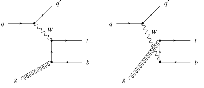
Figure 2: Single-top-quark production via $W$-gluon fusion.

At the Fermilab Tevatron ($\sqrt{S}$ = 2 TeV $p\bar{p}$ collider), the sum of the cross sections for $q\bar{q}\to t\bar{b}$ and $q\bar{q}\to\bar{t}b$ is roughly a factor of seven smaller than the dominant $t\bar{t}$ production cross section [7], and about a factor of two smaller than the $W$-gluon-fusion cross section [6]. Nevertheless, a recent study indicates that with double $b$ tagging, a signal is observable at the Tevatron with 2-3 fb^-1 of integrated luminosity [3]. Unfortunately, even though the $q\bar{q}\to t\bar{b},\bar{t}b$ cross section is larger at the CERN Large Hadron Collider (LHC, $\sqrt{S}$ = 14 TeV $pp$ collider), the signal will likely be obscured by backgrounds from the even larger $t\bar{t}$ and $W$-gluon fusion processes, which are initiated by gluons [3].

An important feature of $q\bar{q}\to t\bar{b}$ is the accuracy with which the cross section can be calculated. The top-quark mass is much larger than $\Lambda_{QCD}$, so calculations are performed in a regime where perturbative QCD is very reliable. The correction to the initial state is identical to that occurring in the ordinary Drell-Yan process $q\bar{q}\to W^{*}\!\to\bar{\ell}\nu$ ($W^{*}$ denotes a virtual $W$ boson), which has been calculated to ${\sl O}(\alpha_{s}^{2})$ [8]. Furthermore, by experimentally measuring $q\bar{q}\to W^{*}\to\bar{\ell}\nu$, the initial quark-antiquark flux can be constrained without recourse to perturbation theory. This provides a check of the parton distribution functions, and allows the reduction of systematic errors. The parton distribution functions are not expected to be a large source of uncertainty, as the dominant contribution to the cross section comes from quark and antiquark distribution functions evaluated at relatively high values of $x$, where they are well known. There is little sensitivity to the less-well-known gluon distribution function, in contrast to the case of $W$-gluon fusion. The final-state correction to the inclusive cross section is straightforward, and involves no collinear or infrared singularities. The QCD corrections to the initial and final states do not interfere at next-to-leading-order because the $t\bar{b}$ is in a color singlet if a gluon is emitted from the initial state, but a color octet if it is emitted from the final state. There is, however, interference at ${\sl O}(\alpha_{s}^{2})$ from the emission of two gluons.

This paper is organized as follows. In Section 2 we present the ${\sl O}(\alpha_{s})$ QCD corrections to both the initial and final states, and discuss their dependence on the renormalization and factorization scales. In Section 3 we present the ${\sl O}(\alpha_{W}m_{t}^{2}/M_{W}^{2})$ Yukawa correction. In Section 4 we present a summary of our results. We give an analytic expression for the Yukawa correction in an appendix.

2 QCD correction

The diagrams which contribute to the ${\sl O}(\alpha_{s})$ correction to $q\bar{q}\to t\bar{b}$ are shown in Fig. 3. As mentioned in the Introduction, the QCD corrections to the initial and final states do not interfere at ${\sl O}(\alpha_{s})$. Therefore, we may consider the corrections to the initial and final states separately. To this end, we break up the process $p\bar{p}\to t\bar{b}+X$ into the production of a virtual $W$ boson of mass-squared $q^{2}$, followed by its propagation and decay into $t\bar{b}$.

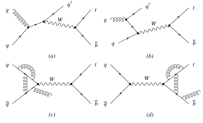
Figure 3: ${\sl O}(\alpha_{s})$ correction to $q\bar{q}\to t\bar{b}$: (a)-(c) initial state, (d) final state.

The production cross section of the virtual $W$ boson is formally identical to that of the Drell-Yan process, to all orders in QCD. The modulus squared of the decay amplitude of the virtual $W$ boson, integrated over the phase space of all final-state particles, is obtained by the application of Cutkosky’s rules [9] as twice the imaginary part of the self-energy of the $W$ boson due to a $t\bar{b}$ loop, again to all orders in QCD. Furthermore, because the current to which the $W$ boson couples in the initial state is conserved to all orders in QCD (for massless quarks), we need only consider the $-g^{\mu\nu}$ term in the $W$-boson propagator and self-energy. Thus we may write the differential cross section as

$$\frac{d\sigma}{dq^{2}}(p\bar{p}\to t\bar{b}+X)=\sigma(p\bar{p}\to W^{*}\!+X)\frac{{\rm Im}\>\Pi(q^{2},m_{t}^{2},m_{b}^{2})}{\pi(q^{2}-M_{W}^{2})^{2}}$$ (1)

where $\Pi$ is the coefficient of the $-g^{\mu\nu}$ term of the self-energy of a $W$ boson with mass-squared $q^{2}$. The total cross section is obtained by integrating over $q^{2}$. This equation is valid to ${\sl O}(\alpha_{s})$, but not beyond, because it neglects the interference between the QCD corrections to the initial and final states.

To demonstrate this procedure, we obtain the leading-order cross section for $p\bar{p}\to t\bar{b}$ using

$$\sigma(p\bar{p}\to W^{*}\!+X) = \sum_{i,j}\int dx_{1}\int dx_{2}\,[q_{i}(x_{1},\mu_{F})\bar{q}_{j}(x_{2},\mu_{F})+\bar{q}_{i}(x_{1},\mu_{F})q_{j}(x_{2},\mu_{F})]$$

$$\times|V_{ij}|^{2}\frac{\pi^{2}\alpha_{W}}{3}\delta(x_{1}x_{2}S-q^{2})$$

where $\alpha_{W}=g^{2}/4\pi\equiv\sqrt{2}G_{\mu}M_{W}^{2}/\pi$, $S$ is the square of the total hadronic center-of-mass energy, $q$ and $\bar{q}$ are the parton distribution functions, $\mu_{F}$ is the factorization scale, and the sum on $i$ and $j$ runs over all contributing quark-antiquark combinations. At leading order, the coefficient of the $-g^{\mu\nu}$ term in the imaginary part of the $W$-boson self-energy is

$${\rm Im}\>\Pi(q^{2},m_{t}^{2},m_{b}^{2})=\frac{\alpha_{W}\lambda^{1/2}|V_{tb}|^{2}}{2}\left[1-\frac{m_{t}^{2}+m_{b}^{2}}{2q^{2}}-\frac{(m_{t}^{2}-m_{b}^{2})^{2}}{2q^{4}}\right]$$ (3)

where $\lambda$ is the triangle function associated with two-particle phase space,

$$\lambda=\lambda(q^{2},m_{t}^{2},m_{b}^{2})=q^{4}+m_{t}^{4}+m_{b}^{4}-2q^{2}m_{t}^{2}-2q^{2}m_{b}^{2}-2m_{t}^{2}m_{b}^{2}\;.$$ (4)

Using Eq. (1), the differential cross section is thus

$$\frac{d\sigma}{dq^{2}}(p\bar{p}\to t\bar{b}+X) = \sum_{i,j}\int dx_{1}\int dx_{2}\,[q_{i}(x_{1},\mu_{F})\bar{q}_{j}(x_{2},\mu_{F})+\bar{q}_{i}(x_{1},\mu_{F})q_{j}(x_{2},\mu_{F})]$$

$$\times|V_{ij}|^{2}\frac{\pi\alpha_{W}^{2}\lambda^{1/2}|V_{tb}|^{2}}{12(q^{2}-M_{W}^{2})^{2}}\left[1-\frac{m_{t}^{2}+m_{b}^{2}}{2q^{2}}-\frac{(m_{t}^{2}-m_{b}^{2})^{2}}{2q^{4}}\right]\delta(x_{1}x_{2}S-q^{2})\;.$$

At leading order, the integration over $q^{2}$ to obtain the total cross section is trivial due to the delta function. At next-to-leading order, however, it is necessary to perform the integration numerically.

The ${\sl O}(\alpha_{s})$ corrections to the Drell-Yan process [10] and the $W$-boson self energy [11, 12] were both calculated many years ago. We use the expression for $\sigma(p\bar{p}\to W^{*}+X)$ as given in Eqs. (9.5) and (12.3) of Ref. [13], and Im $\Pi$ as derived from Eq. (3.3) of Ref. [12]. We use $m_{t}$ = 175 GeV, $m_{b}$ = 5 GeV, $M_{W}$ = 80.33 GeV, $|V_{tb}|$ = 1, $G_{\mu}=1.16639\times 10^{-5}\;{\rm GeV}^{-2}$, and $\alpha_{s}$ as given by the parton distribution functions.

The calculation of the initial-state correction includes divergences arising from collinear parton emission. These divergences cancel with corresponding divergences present in the QCD correction to the parton distribution functions. The finite terms remaining depend on the factorization scale $\mu_{F}$, both through the parton distribution functions and explicitly in the partonic cross section. The variation of the leading-order and next-to-leading-order cross sections with $\mu_{F}/\sqrt{q^{2}}$, where $\sqrt{q^{2}}$ is the mass of the virtual $W$ boson, is shown in Fig. 4 at both the Tevatron and the LHC. The leading-order cross section is calculated with the CTEQ3L leading-order parton distribution functions, and the next-to-leading-order cross section with the CTEQ3M next-to-leading-order parton distribution functions [14]. The leading-order cross section varies considerably with $\mu_{F}$, while the next-to-leading-order cross section is appreciably less sensitive. The next-to-leading-order cross section shown in Fig. 4 contains only the initial-state correction. We see that for $\mu_{F}=\sqrt{q^{2}}$ the initial-state correction is +36% at the Tevatron and +33% at the LHC. In what follows, we set $\mu_{F}=\sqrt{q^{2}}$.

Figure 4: Factorization-scale dependence of the leading-order (LO) and next-to-leading-order (NLO) cross sections for $q\bar{q}\to t\bar{b},\bar{t}b$ at the Tevatron and the LHC. The NLO cross sections include only the initial-state QCD correction, and not the final-state correction. The LO cross sections are calculated with the CTEQ3L LO parton distribution functions, and the NLO cross sections with the CTEQ3M NLO parton distribution functions.

The cross section at next-to-leading order also depends on the renormalization scale, $\mu_{R}$, at which $\alpha_{s}$ is evaluated. In Fig. 5 we show the next-to-leading-order cross section, including both initial- and final-state corrections, as a function of $\mu_{R}/\sqrt{q^{2}}$, at both the Tevatron and the LHC. The dependence of the cross section on the renormalization scale first appears at next-to-leading order and is therefore mild. In what follows, we set $\mu_{R}=\sqrt{q^{2}}$. The final-state correction increases the cross section by $+18\%$ of the leading-order cross section at the Tevatron and $+17\%$ at the LHC.

Figure 5: Renormalization-scale dependence of the leading-order (LO) and next-to-leading-order (NLO) cross sections for $q\bar{q}\to t\bar{b},\bar{t}b$ at the Tevatron and the LHC. The NLO cross sections include both the initial-state and final-state correction. The LO cross sections are calculated with the CTEQ3L LO parton distribution functions, and the NLO cross sections with the CTEQ3M NLO parton distribution functions.

We show in Fig. 6 the leading-order and next-to-leading-order differential cross section as a function of the mass of the virtual $W$ boson, $\sqrt{q^{2}}$, at both the Tevatron and the LHC. Also shown are the separate ${\sl O}(\alpha_{s})$ corrections from the initial and final states. These corrections have different shapes from the leading-order cross section, and from each other. In order to observe $t\bar{b}$ production experimentally, it is necessary to detect the $\bar{b}$ quark [3]. Thus the measured cross section will exclude some region near threshold, where the $\bar{b}$ quark does not have sufficient transverse momentum to be detected with high efficiency. Therefore the measured cross section, as well as the QCD correction, will depend on the acceptance for the $\bar{b}$ quark.

Figure 6: Differential cross section for $q\bar{q}\to t\bar{b},\bar{t}b$ versus the mass of the virtual $s$-channel $W$ boson, at the Tevatron and the LHC. Both the leading-order (LO) and next-to-leading order (NLO) cross sections are shown, as well as the separate contributions from the initial-state (IS) and final-state (FS) corrections. The LO cross sections are calculated with the CTEQ3L LO parton distribution functions, and the NLO cross sections with the CTEQ3M NLO parton distribution functions.

If the top and bottom quarks were stable, they would form quarkonium bound states just below threshold [15]. We estimate the distance below threshold that the ground state would occur, by analogy with the hydrogen atom, to be $E\approx(4\alpha_{s}/3)^{2}m_{b}/2\approx 50$ MeV. The formation time of the ground state is approximately $1/E$. This is much greater than the top-quark lifetime, $\Gamma_{t}^{-1}\approx(1.5\>{\rm GeV})^{-1}$, so there is not sufficient time for quarkonium bound states to form [16].

Because the top-quark width is small compared to its mass, interference between the corrections to production and decay amplitudes has a negligible effect, of order $\alpha_{s}\Gamma_{t}/m_{t}$, on the total cross section [17]. This interference also has a negligible effect on differential cross sections, such as the invariant-mass distribution of the decay products of the top quark [18].

Our final results for the cross section and uncertainty will be presented in Section 4.

3 Yukawa correction

The diagrams which contribute to the ${\sl O}(\alpha_{W}m_{t}^{2}/m_{W}^{2})$ Yukawa correction to $q\bar{q}\to t\bar{b}$ are shown in Fig. 7. The dashed lines represent the Higgs boson and the unphysical scalar $W$ and $Z$ bosons associated with the Higgs field (in the $R_{\xi}$ gauge). The effect of a top-quark loop in the $W$-boson propagator, which might be expected to contribute a term of Yukawa strength, is absorbed by the renormalized weak coupling constant, which we express in terms of $G_{\mu}$, the Fermi constant measured in muon decay ($\alpha_{W}=g^{2}/4\pi\equiv\sqrt{2}G_{\mu}M_{W}^{2}/\pi$). We use standard Feynman integral techniques with dimensional regularization to calculate the loop diagrams [19], and work in the approximation where the bottom quark is massless. Our other parameters are $m_{t}$ = 175 GeV, $M_{W}$ = 80.33 GeV, $|V_{tb}|$ = 1, and $G_{\mu}=1.16639\times 10^{-5}\;{\rm GeV}^{-2}$.

Figure 7: ${\sl O}(\alpha_{W}m_{t}^{2}/M_{W}^{2})$ corrections to $q\bar{q}\to t\bar{b}$. The dashed lines represent the Higgs boson and the unphysical scalar $W$ and $Z$ bosons (in $R_{\xi}$ gauge): (a) wavefunction renormalization, (b) vertex correction.

In the $m_{b}=0$ approximation, the matrix element of the $t\bar{b}$ current may be written as

$$i\bar{u}(p_{t})\Gamma^{\mu A}v(p_{b}) = \left(\frac{-igT^{A}}{2\sqrt{2}}\right)\left\{\bar{u}(p_{t})\gamma^{\mu}(1-\gamma^{5})v(p_{b})\frac{}{}\right.$$

$$\left.+\left(\frac{m_{t}^{2}G_{\mu}}{8\sqrt{2}\pi^{2}}\right)\bar{u}(p_{t})\left[\gamma^{\mu}F_{1}(q^{2})+\frac{(p_{t}^{\mu}-p_{b}^{\mu})}{m_{t}}F_{2}(q^{2})\right](1-\gamma^{5})v(p_{b})\right\}$$

where $p_{t}$ and $p_{b}$ are the outgoing four-momenta of the $t$ and $\bar{b}$ quarks, respectively; the form factors $F_{1}$ and $F_{2}$ are functions of $q^{2}=(p_{t}+p_{b})^{2}$ and the Higgs-boson mass; and $T^{A}$ is an SU(3) matrix [Tr$(T^{A}T^{B})=\frac{1}{2}\delta^{AB}$]. The fractional change in the differential cross section as a function of the $q^{2}$ of the virtual $W$ boson is

$$\frac{\Delta d\sigma_{Y}/d\sqrt{q^{2}}}{d\sigma_{LO}/d\sqrt{q^{2}}}=\left(\frac{m_{t}^{2}G_{\mu}}{8\sqrt{2}\pi^{2}}\right)\left[2F_{1}(q^{2})+F_{2}(q^{2})\frac{(q^{2}-m_{t}^{2})^{2}}{q^{4}-\frac{1}{2}q^{2}m_{t}^{2}-\frac{1}{2}m_{t}^{4}}\right]\;.$$ (7)

Analytic expressions for the form factors $F_{1}$ and $F_{2}$ are given in an appendix.

The fractional change in the total cross section, $\Delta\sigma_{Y}/\sigma_{LO}$, is plotted in Fig. 8 vs. the Higgs-boson mass, $M_{H}$, at both the Tevatron and the LHC. For values of $M_{H}$ between 60 GeV and 1 TeV, the absolute value of the Yukawa correction is never more than one percent of the leading-order cross section. Thus the Yukawa correction is negligible for this process, as has also been found to be the case for $t\bar{t}$ production [20, 21]. Since $W$-gluon fusion also involves the $t\bar{b}$ weak charged current, our calculation suggests that the Yukawa correction to that process is also negligible. As previously mentioned, the ordinary weak correction is expected to be comparable to the Yukawa correction, so it too should be negligible. The Yukawa correction could potentially be much larger in models with enhanced couplings of Higgs bosons to top or bottom quarks [20, 22].

Figure 8: Fractional change in the total cross section for $q\bar{q}\to t\bar{b},\bar{t}b$ due to the Yukawa correction vs. the Higgs-boson mass at the Tevatron and the LHC.

4 Conclusions

The cross section for $q\bar{q}\to t\bar{b},\bar{t}b$ at both the Tevatron and the LHC is given in Table 1. The leading-order cross section, next-to-leading-order cross section including only the initial-state QCD correction, and the full next-to-leading order cross section are given. The factorization and renormalization scales are both set equal to $\sqrt{q^{2}}$, the mass of the virtual $W$ boson. We give results for three different sets of next-to-leading-order parton distribution functions: CTEQ3M [14], MRS(A${}^{{}^{\prime}}$), and MRS(G) [23]. The QCD correction to the cross section is significant: about $+54\%$ at the Tevatron and $+50\%$ at the LHC, with the leading-order cross section evaluated with leading-order parton distribution functions, and the next-to-leading-order cross section evaluated with next-to-leading-order parton distribution functions. The size of the ${\cal O}(\alpha_{s})$ correction improves the outlook for observation of this process in Run II at the Tevatron.

$m_{t}=175\;{\rm GeV},\mu_{R}=\mu_{F}=\sqrt{q^{2}}$		CTEQ3L,3M	MRS(A′)	MRS(G)
	$\sigma_{LO}$	.578	.601	.602
Tevatron	$\sigma_{NLO(IS)}$	.789	.766	.758
$\sqrt{S}$ = 2 TeV	$\sigma_{NLO}$	.894	.868	.860
	$\sigma_{\bf NLO}$ (avg) = .88 $\pm$ .05 pb
	$\sigma_{LO}$	6.76	7.83	7.81
LHC	$\sigma_{NLO(IS)}$	9.02	9.01	9.03
$\sqrt{S}$ = 14 TeV	$\sigma_{NLO}$	10.19	10.17	10.21
	$\sigma_{\bf NLO}$ (avg) = 10.2 $\pm$ 0.6 pb

Table 1: Leading-order (LO) and next-to-leading-order (NLO) cross sections (pb) for $q\bar{q}\to t\bar{b},\bar{t}b$ at the Tevatron and the LHC for three different sets of parton distribution functions (PDFs). The NLO cross section including only the initial state (IS) correction is also given. The CTEQ LO cross section is computed with the CTEQ3L LO PDFs; all other cross sections are computed with NLO PDFs. The final NLO cross section is the average of the CTEQ3M and MRS(A^′) cross sections, with an uncertainty of $\pm 6\%$, as discussed in the text.

As shown in Fig. 4, varying the factorization scale between one half and twice $\sqrt{q^{2}}$ changes the cross section by only $\pm 2\%$. Varying the renormalization scale over this same range yields a similar change in the cross section, as shown in Fig. 5. Using these results to estimate the contribution from higher-order QCD corrections, we conclude that the uncertainty in the cross section is at the level of $\pm 4\%$. This conclusion is supported by the known next-to-next-to-leading-order correction to the Drell-Yan process, which is about $2\%$ (in the modified minimal subtraction ($\overline{\rm MS}$) scheme) [8].

It is difficult to reliably ascertain the uncertainty in the cross section from the parton distribution functions at this time. The small difference in the next-to-leading-order cross sections using MRS(A${}^{{}^{\prime}}$) and MRS(G) supports the contention that the calculation is insensitive to the gluon distribution function. The difference between the cross section using CTEQ3M and MRS(A${}^{{}^{\prime}}$) suggests that the uncertainty in the cross section from the parton distribution functions is on the order of $\pm 2\%$. However, since each set of parton distribution functions represents the best fit to some set of data, the uncertainty is certainly larger than this. Therefore, we assign an uncertainty of $\pm 4\%$ from the parton distribution functions.

For our final estimate, we average the next-to-leading-order cross sections using the CTEQ3M and MRS(A${}^{{}^{\prime}}$) parton distribution functions. We assign an uncertainty of $\pm 6\%$, which reflects the uncertainties above, added in quadrature. We quote as our final result for $q\bar{q}\to t\bar{b},\bar{t}b$ a cross section of $.88\pm.05$ pb at the Tevatron, and $10.2\pm 0.6$ pb at the LHC.

An additional source of uncertainty is the top-quark mass. A plot of the next-to-leading order cross section for $q\bar{q}\to t\bar{b},\bar{t}b$ as a function of the top-quark mass is show in Fig. 9. It is anticipated that this uncertainty will be $\pm 6$ GeV when the data from Run I at the Tevatron are fully analyzed. This yields an uncertainty of $\pm 15\%$ in the cross section at the Tevatron. The uncertainty in the mass is expected to decrease to $\pm 4$ GeV in Run II [24], corresponding to an uncertainty in the cross section of $\pm 10\%$. A high-luminosity Tevatron might be capable of reducing the uncertainty in the mass to $\pm 2$ GeV [24], which would yield an uncertainty in the cross section of $\pm 5\%$. The uncertainty in the cross section at the LHC is comparable.

Figure 9: Next-to-leading order cross section for $q\bar{q}\to t\bar{b},\bar{t}b$ as a function of the top-quark mass.

Much can be done to reduce the uncertainty in the calculation. The next-to-next-to-leading-order correction to the Drell-Yan process is already known [8]. The full next-to-next-to-leading-order QCD correction to $q\bar{q}\to t\bar{b}$ can and should be completed in the near future. This should reduce the uncertainty in the cross section from yet higher orders to below the $1\%$ level. A reliable estimate of the uncertainty in the parton distribution functions requires a set with built-in uncertainties, which we hope will be available in the near future.

It seems likely that by the time the process $q\bar{q}\to t\bar{b}$ is observed in Run II at the Tevatron, the theoretical uncertainty in the cross section will be slightly larger than $\pm 10\%$, due mostly to the uncertainty in the mass. This is adequate in comparison with the anticipated experimental errors. The statistical error on the measured cross section in Run II will be about $\pm 20\%$ [3]. This corresponds to a measurement of $|V_{tb}|$ with an accuracy of $\pm 10\%$ (assuming $|V_{tb}|\approx 1$). A high-luminosity Tevatron, which could potentially deliver 30 fb^-1 over several years, would allow a measurement of the cross section with a statistical uncertainty of about $6\%$, with a comparable theoretical uncertainty. Combining the statistical and theoretical uncertainties in quadrature, this corresponds to a measurement of $|V_{tb}|$ with an accuracy of about $\pm 4\%$.

The process $q\bar{q}\to t\bar{b}$ is also important as a background to the process $q\bar{q}\to WH$ with $H\to b\bar{b}$ at the Tevatron. We show in Fig. 10 the next-to-leading-order cross sections for $q\bar{q}\to W^{\pm}H$, as well as $q\bar{q}\to ZH$, at both the Tevatron and the LHC [25]. The significant increase in the $q\bar{q}\to t\bar{b}$ cross section at next-to-leading order could have a negative impact on the ability to find an intermediate-mass Higgs boson at the Tevatron.

Figure 10: Cross section for $q\bar{q}\to W^{\pm}H$ and $q\bar{q}\to ZH$ at the Tevatron and the LHC, calculated at next-to-leading order using CTEQ3M parton distribution functions.

Appendix

Below are the form factors for the Yukawa correction to the matrix element of the $t\bar{b}$ charged current. These corrections arise from loops of Higgs bosons and the unphysical scalar $W$ and $Z$ bosons associated with the Higgs field in the $R_{\xi}$ gauges. The masses-squared of the unphysical scalar bosons are $\xi M_{W}^{2},\xi M_{Z}^{2}$. In the numerical calculations, we set $\xi=0$ (Landau gauge). The integrals were reduced to the standard one-, two-, and three-point scalar loop integrals and then evaluated with the aid of the code FF [26]. The notation is adopted from [19]; the arguments of the functions give the internal masses-squared followed by the external momenta squared.

$$F_{1} = {\small\frac{1}{2}}[4C_{24}(\xi M_{W}^{2},M_{H}^{2},m_{t}^{2};q^{2},m_{t}^{2},0)+4C_{24}(\xi M_{W}^{2},\xi M_{Z}^{2},m_{t}^{2};q^{2},m_{t}^{2},0)$$

$$\mbox{}+B_{1}(M_{H}^{2},m_{t}^{2};m_{t}^{2})+(M_{H}^{2}-4m_{t}^{2})B_{0}^{{}^{\prime}}(M_{H}^{2},m_{t}^{2};m_{t}^{2})$$

$$\mbox{}+B_{1}(\xi M_{Z}^{2},m_{t}^{2};m_{t}^{2})+\xi M_{Z}^{2}B_{0}^{{}^{\prime}}(\xi M_{Z}^{2},m_{t}^{2};m_{t}^{2})$$

$$\mbox{}+B_{1}(\xi M_{W}^{2},0;m_{t}^{2})+(\xi M_{W}^{2}-m_{t}^{2})B_{0}^{{}^{\prime}}(\xi M_{W}^{2},0;m_{t}^{2})$$

$$\mbox{}+B_{1}(\xi M_{W}^{2},m_{t}^{2};0)+(\xi M_{W}^{2}+m_{t}^{2})B_{0}^{{}^{\prime}}(\xi M_{W}^{2},m_{t}^{2};0)]$$

$$F_{2} = m_{t}^{2}[C_{23}(\xi M_{W}^{2},M_{H}^{2},m_{t}^{2};q^{2},m_{t}^{2},0)+C_{23}(\xi M_{W}^{2},\xi M_{Z}^{2},m_{t}^{2};q^{2},m_{t}^{2},0)$$

$$\mbox{}+C_{21}(\xi M_{W}^{2},M_{H}^{2},m_{t}^{2};q^{2},m_{t}^{2},0)+C_{21}(\xi M_{W}^{2},\xi M_{Z}^{2},m_{t}^{2};q^{2},m_{t}^{2},0)$$

$$\mbox{}+2C_{11}(\xi M_{W}^{2},M_{H}^{2},m_{t}^{2};q^{2},m_{t}^{2},0)]$$

Note: In the reduction of the three-point integrals, a misprint was discovered in Ref. [19]. On p. 199 in Appendix E, in an unnumbered equation near the bottom of the page, $C_{22}$ and $C_{23}$ were transposed. The correct equation is $(C_{23},C_{22})=X^{-1}(R_{4},R_{6})$.

References

- [1] CDF Collaboration, F. Abe et al., Phys. Rev. Lett. 74, 2626 (1995); D0 Collaboration, S. Abachi et al., Phys. Rev. Lett. 74, 2632 (1995).
- [2] S. Cortese and R. Petronzio, Phys. Lett. B253, 494 (1991).
- [3] T. Stelzer and S. Willenbrock, Phys. Lett. B357, 125 (1995).
- [4] Review of Particle Properties, R.M. Barnett et al., Phys. Rev. D 54, 1 (1996).
- [5] A. Stange, W. Marciano, and S. Willenbrock, Phys. Rev. D 49, 1354 (1994); Phys. Rev. D 50, 4491 (1994); A. Belyaev, E. Boos, and L. Dudko, Mod. Phys. Lett. A10, 25 (1995); S. Mrenna and G. Kane, CALT-68-1938 (1994); D. Froidevaux and E. Richter-Was, Z. Phys. C67, 213 (1995).
- [6] S. Willenbrock and D. Dicus, Phys. Rev. D 34, 155 (1986); C.-P. Yuan, Phys. Rev. D 41, 42 (1990); D. Carlson and C.-P. Yuan, Phys. Lett. B306, 386 (1993); R. K. Ellis and S. Parke, Phys. Rev. D 46, 3785 (1992); G. Bordes and B. van Eijk, Nucl. Phys. B435, 23 (1995); A. Heinson, A. Belyaev, and E. Boos, hep-ph/9509274.
- [7] P. Nason, S. Dawson, and R. K. Ellis, Nucl. Phys. B303, 607 (1988); W. Beenakker, H. Kuijf, W. van Neerven, and J. Smith, Phys. Rev. D 40, 54 (1989); E. Laenen, J. Smith, and W. van Neerven, Nucl. Phys. B369, 543 (1992); Phys. Lett. B321, 254 (1994); E. Berger and H. Contopanagos, Phys. Lett. B361, 115 (1995); hep-ph/9603326; S. Catani, M. Mangano, P. Nason, and L. Trentadue, hep-ph/9602208; hep-ph/9604351.
- [8] R. Hamberg, W. van Neerven, and T. Matsuura, Nucl. Phys. B359, 343 (1991); W. van Neerven and E. Zijlstra, Nucl. Phys. B382, 11 (1992).
- [9] R. Cutkosky, J. Math Phys. 1, 429 (1960).
- [10] G. Altarelli, R. K. Ellis and G. Martinelli, Nucl. Phys. B157, 461 (1979); J. Kubar-André and F. Paige, Phys. Rev. D 19, 221 (1979).
- [11] K. Schilcher, M. Tran, and N. Nasrallah, Nucl. Phys. B181, 91 (1981).
- [12] T. Chang, K. Gaemers and W. van Neerven, Nucl. Phys. B202, 407 (1982).
- [13] S. Willenbrock, in From Actions to Answers, Proc. 1989 Theoretical Advanced Study Institute (TASI), eds. T. DeGrand and D. Toussaint (World Scientific, Singapore, 1990).
- [14] H. Lai, J. Botts, J. Huston, J. Morfin, J. Owens, J. Qiu, W.-K. Tung, and H. Weerts, Phys. Rev. D 51, 4763 (1995).
- [15] G. Couture and M. Praszalowicz, Phys. Lett. B229, 139 (1989).
- [16] V. Fadin and V. Khoze, JETP Lett. 46, 525 (1987); Sov. J. Nucl. Phys. 48, 309 (1988).
- [17] V. Fadin, V. Khoze, and A. Martin, Phys. Rev. D 49, 2247 (1994).
- [18] R. Pittau, hep-ph/9603265.
- [19] G. Passarino and M. Veltman, Nucl. Phys. B160, 151 (1979).
- [20] A. Stange and S. Willenbrock, Phys. Rev. D 48, 2054 (1993).
- [21] W. Beenakker, A. Denner, W. Hollik, R. Mertig, T. Sack, and D. Wackeroth, Nucl. Phys. B411, 343 (1994).
- [22] C. Kao, Phys. Lett. B348, 155 (1995).
- [23] A. Martin, R. Roberts, and W. J. Stirling, Phys. Lett. B354, 155 (1995).
- [24] Report of the TeV-2000 Study Group, eds. D. Amidei and R. Brock, Fermilab-Pub-96/082 (1996).
- [25] T. Han and S. Willenbrock, Phys. Lett. B273, 167 (1991).
- [26] G. J. van Oldenborgh, Comput. Phys. Commun. 66, 1 (1991).