LBL-38549

Parton Model Sum Rules

Ian Hinchliffe and Axel Kwiatkowski

Theoretical Physics Group
Ernest Orlando Lawrence Berkeley National Laboratory
University of California
Berkeley, California 94720

This review article discusses the experimental and theoretical status of various Parton Model sum rules. The basis of the sum rules in perturbative QCD is discussed. Their use in extracting the value of the strong coupling constant is evaluated and the failure of the naive version of some of these rules is assessed.

Disclaimer

This document was prepared as an account of work sponsored by the United States Government. While this document is believed to contain correct information, neither the United States Government nor any agency thereof, nor The Regents of the University of California, nor any of their employees, makes any warranty, express or implied, or assumes any legal liability or responsibility for the accuracy, completeness, or usefulness of any information, apparatus, product, or process disclosed, or represents that its use would not infringe privately owned rights. Reference herein to any specific commercial products process, or service by its trade name, trademark, manufacturer, or otherwise, does not necessarily constitute or imply its endorsement, recommendation, or favoring by the United States Government or any agency thereof, or The Regents of the University of California. The views and opinions of authors expressed herein do not necessarily state or reflect those of the United States Government or any agency thereof, or The Regents of the University of California.

Lawrence Berkeley Laboratory is an equal opportunity employer.

1 Introduction

One of the best tools to use in attempting to disentangle the structure of the nucleon is lepton-nucleon scattering where the lepton, whose couplings to electroweak gauge bosons is fully known, is used as a probe on the constituents of the nucleon. Lepton-nucleon scattering with large momentum transfer between the lepton and the nucleon is described in terms of the Parton Model [1, 2]. In its naive form this model describes the nucleon as a collection of non-interacting quarks and gluons. Lepton-nucleon scattering is then viewed as the sum of incoherent scatterings by the lepton off these partonic constituents. The description of these constituents is most conveniently given in a frame where the nucleon has large momentum. If the nucleon mass is neglected, its momentum can be written as $P^{\mu}=(p,p,0,0)$. A parton momentum can be written as $P^{\mu}_{i}=(z_{i}p,z_{i}p,p_{t},0)$ where $p_{t}\sim 300$ MeV is related to the scale of nucleon binding. A distribution function $f_{i}(z)$ is defined so that the probability that a parton of type $i$ (for example an up quark) has momentum in the range $P(z)$ to $P(z+dz)$ is $f_{i}(z)$. The lepton-nucleon scattering rates are then expressed in terms of $f_{i}$.

The target nucleon is characterised by certain quantum numbers such as isospin and baryon number. These quantum numbers are carried by the constituents. For example, the net number of up quarks in a proton is two, hence $\int_{0}^{1}dz(f_{u}(z)-f_{\overline{u}}(z))=2$. By forming appropriate combinations of scattering cross-sections, quantities can be measured that correspond to these conserved quantum numbers and hence have simple values in the Naive Parton Model. These quantities are referred to as Parton Model sum rules. They can then be compared with experiment and the fundamental properties of theory tested. This Naive Parton Model is subject to corrections in the full theory of strong interactions (Quantum Chromodynamics or QCD [3, 4], for recent reviews see [5, 6, 7] ). These corrections fall into two types; those that are strongly suppressed at high energy (higher twist corrections) and those that vanish only logarithmically with the momentum transfer. The latter are fully calculable in terms of the coupling constant $\alpha_{s}$ of QCD. Comparison of the sum rules with these QCD expectations then provides a powerful test of QCD and enables $\alpha_{s}$ to be measured.

In the remainder of this article we will discuss these sum rules. We show their values in the Naive Parton Model and the corrections from QCD and finally compare these predicted values with experiment.

1.1 Deep Inelastic Scattering

The kinematics of lepton-nucleon scattering are shown in Figure 1. The scattering of an unpolarized charged lepton (an electron or muon) or neutrino of momentum $k$ off an unpolarized nucleon of mass $M$, momentum $P$ results in a final state with a lepton of momentum $k^{\prime}$ and a nuclear fragment.

Figure 1: Diagram illustrating the deep inelastic scattering process electron + proton $\to$ electron + anything.

The inclusive cross-section for this process can be described by two Lorentz scalars which can be taken to be $Q^{2}=-(k^{\prime}-k)^{2}$ and $\nu=P\cdot(k-k^{\prime})$. Convenient dimensionless variables are $x=Q^{2}/2\nu$ and $y=\nu/P\cdot k$ both of which range from zero to one. The latter is the fractional energy loss of the lepton in the rest frame of the nucleon. Two types of scattering are important, neutral and charged current scattering. The former case describes the process $\mu N\to\mu X$ or $eN\to eX$. For neutral current scattering and $Q^{2}<<M_{Z}^{2}$ (all of the data discussed in this article satisfy this requirement), the cross-section can be expressed as

$$\begin{array}[]{rl}\displaystyle\frac{d\sigma^{eN}}{dxdy}&=\displaystyle\frac{4\pi\alpha_{em}^{2}}{sx^{2}y^{2}}\cr\displaystyle(xy^{2}F_{1}^{eN}(x,Q^{2})&+(1-y-M^{2}x^{2}y^{2}/Q^{2})F_{2}^{eN}(x,Q^{2}))\end{array}$$ (1)

where $s=(P+k)^{2}$ and $F_{1},F_{2}$ are arbitrary functions called structure functions. This is the most general form that this cross-section can take consistent with Lorentz invariance and parity conservation provided that terms that are proportional to quark masses (actually $m_{q}^{2}/Q^{2}$) are neglected. This is an excellent approximation since the nucleon consists mainly of up, down and strange quarks that have very small masses ($m_{u}\sim m_{d}\sim\hbox{few}$ MeV and $m_{s}\sim 100$ MeV [8]). For charged current scattering, the presence of parity violation which proceeds via the exchange of a $W$ boson between the lepton and the target nucleon, requires the appearance of another function $F_{3}$.

$$\begin{array}[]{ll}\displaystyle\frac{d\sigma^{\nu N}}{dxdy}=&\displaystyle\frac{G_{F}^{2}M_{W}^{4}s}{2\pi(Q^{2}+M_{W}^{2})^{2}}(xy^{2}F_{1}^{\nu N}(x,Q^{2})\cr&\displaystyle+(1-y-x^{2}y^{2}M^{2}/Q^{2})F_{2}^{\nu N}(x,Q^{2})\cr&\displaystyle-\frac{1}{2}x((1-y)^{2}-1)F_{3}^{\nu N}(x,Q^{2}))\end{array}$$ (2)

For $\overline{\nu}N$ scattering the sign of the last ($xF_{3}$) term is reversed. The above formulae assume that the target nucleon and charged lepton are unpolarized (the neutrino is always polarized). In the case of $eN$ scattering with polarized electron and nucleon a parity conserving asymmetry can be formed.

$$a(x,y)=\frac{d\sigma^{eN}_{p}}{dxdy}-\frac{d\sigma^{eN}_{ap}}{dxdy}$$ (3)

where the subscript $p$ ($ap$) refers to the state where the nucleon spin is parallel (anti-parallel) to its direction of motion in the center of mass frame of the lepton-nucleon system. In both cases the lepton has its spin aligned along its direction of motion. Then

$$\begin{array}[]{ll}a(x,y)=&\displaystyle\frac{8\pi\alpha_{em}^{2}y}{MQ^{2}}((1-2/y^{2}+2x^{2}y^{2}M^{2}/Q^{2})G_{1}(x,Q^{2})\\ &+4x^{2}M^{2}G_{2}(x,Q^{2})/Q^{2})\end{array}$$ (4)

defines the spin dependent structure functions $G_{1}$ and $G_{2}$.

In the rest frame of the target nucleon, the various kinematic quantities are related to the energy $E$ ($E^{\prime}$) of the incoming (outgoing) lepton and the scattering angle $\theta$ of the lepton by $y=\nu/ME=(E-E^{\prime})/E$ and $\sin^{2}(\theta/2)=Q^{2}/(4EE^{\prime})$. By measuring the incoming and outgoing lepton energy and the scattering angle the structure functions can be determined.

1.2 Quark Parton Model

In the Quark Parton Model, lepton-nucleon scattering is described by the scattering of a lepton off the partonic (i.e. quark and gluon) constituents of the nucleon. The nucleon structure is described in terms of the parton distribution functions $f_{i}(z)$. We shall often use the following symbols to simplify the notation :- $f_{i}(z)\equiv i(z)$ etc. so that the up quark distribution in a proton is $u(z)$ and the anti-down quark distribution is $\overline{d}(z)$. These distributions will always refer to a proton. When a neutron target is involved we use isospin symmetry to relate the neutron distributions to those of the proton so that the up quark distribution in a neutron is the down quark distribution in the proton and vice-versa, while the gluon ($g(z)$) and the strange, charm, bottom and top distributions ($s(z),c(z),b(z),t(z)$) are the same in proton and neutron. The distribution of these heavier quarks is smaller and in the case of top and to a lesser extent bottom totally negligible. The charm quark is troublesome since its mass cannot be neglected in experiments that have $Q^{2}\sim M_{c}^{2}\sim(1.5\hbox{ GeV})^{2}.$ This effect is most important in neutrino scattering where the process $\nu+s\to\mu^{-}+c$ is a significant part of the cross-section.

Since the quarks carry the quantum numbers of the nucleon these distribution functions satisfy certain constraints. For example, the electric charge of the proton yields

$$1=\int_{0}^{1}dz(\frac{2}{3}(u(z)-\overline{u}(z))-\frac{1}{3}(d(z)-\overline{d}(z))-\frac{1}{3}(s(z)-\overline{s}(z)))$$ (5)

and the zero net strangeness of the proton gives

$$0=\int_{0}^{1}dz(s(z)-\overline{s}(z))$$ (6)

Note that this does not imply that $s(z)=\overline{s}(z)$. Momentum conservation in the lepton-parton scattering process implies that the parton momentum fraction $z$ is identified with the kinematic variable $x$ in the Naive Parton Model. The structure functions $F_{1}$, $F_{2}$ and $F_{3}$ are given in terms of the parton distribution functions. In particular

$$F_{2}(x,Q^{2})^{ep}=x\sum_{i}q_{i}^{2}f_{i}(x)$$ (7)

where $q_{i}$ is the charge of the type $i$ parton. The Naive Parton Model therefore predicts that there is no $Q^{2}$ dependence in $F_{i}(x,Q^{2})$. The partons that couple to the photon and $W$ boson (quarks) have spin $1/2$ and hence $F_{2}(x,Q^{2})=2xF_{1}(x,Q^{2})$, the Callan Gross relationship [9].

The relationships between the structure functions for neutrino scattering and the parton distributions are complicated by the Kobayashi-Maskawa [10] mixing matrix, $V_{ij}$ which determines the relative strength of the coupling of a quark pair to the $W$ boson :- $W^{\mu}\overline{q}_{i}\gamma_{\mu}(1-\gamma_{5})q_{j}V_{ij}$. In order to simplify the results that follow, the equations are written in the approximation that the mixing matrix is a diagonal unit matrix. The mixing can be added by replacing the quark distributions by appropriate linear combinations, for example $d(z)\to(V_{du}+V_{dc}+V_{dt})d(z)$. Neutrino scattering proceeds off up and anti- down type quarks viz $\nu u\to\mu^{+}d$ and $\nu\overline{d}\to\mu^{+}\overline{u}$ leading to the following relations (neglecting top and bottom quark contributions)

$$F_{3}^{\nu p}(x,Q^{2})=2(d(x)-\overline{u}(x)-\overline{c}(x)+s(x))$$ (8)

and

$$F_{2}^{\nu p}(x,Q^{2})=2x(\overline{u}(x)+\overline{c}(x)+d(x)+s(x))$$ (9)

The other relations can be trivially obtained from these. The charm quark contributions will not be written explicitly in the following.

The spin structure of the nucleon is probed in polarized scattering. One can define $\Delta f_{i}(z)$ as the difference between the parton distributions for parton of type $i$ with spins (helicity) parallel and anti parallel to the nucleon’s spin. The unpolarized distributions introduced above are then the sum of these two states. Define the quantities $a_{0}$, $a_{3}$ and $a_{8}$ by

$$\begin{array}[]{ll}a_{0}&\displaystyle=\int_{0}^{1}dx\Big{(}\Delta u+\Delta\bar{u}+\Delta d+\Delta\bar{d}+\Delta s+\Delta\bar{s}\Big{)}\cr\displaystyle a_{3}&\displaystyle=\int_{0}^{1}dx\Big{(}\Delta u+\Delta\bar{u}-\Delta d-\Delta\bar{d}\Big{)}\\ \displaystyle a_{8}&\displaystyle=\frac{1}{\sqrt{3}}\int_{0}^{1}dx\Big{(}\Delta u+\Delta\bar{u}+\Delta d+\Delta\bar{d}-2\Delta s-2\Delta\bar{s}\Big{)}\\ \displaystyle\end{array}$$ (10)

These quantities are related to the matrix elements of the axial vector current between nucleon states. The matrix elements involving changes of flavor can be determined from weak decays. $a_{3}$ is determined from neutron $\beta$-decay: $a_{3}=g_{A}=\frac{G_{V}}{G_{A}}=1.2573\pm 0.0028$. $a_{8}$ and $a_{3}$ can be constrained from the weak decay constants of ($\Sigma,\Lambda$ and $\Xi$) hyperons [11]. Assuming $SU(3)_{F}$ symmetry for the octet axial vector currents this gives $F=(\sqrt{3}a_{8}+a_{3})/4=0.459\pm 0.008$ and $D=\sqrt{3}(\sqrt{3}a_{3}-a_{8})/4=0.798\pm 0.008$ implying $a_{8}=0.33\pm 0.02$ [12]. Data from $\nu p$ and $\overline{\nu}p$ elastic scattering [13] provide information on the matrix element of the flavor singlet current $a_{0}$ to be determined [14, 15]. These data do not directly measure the static quantities and a form factor behaviour must be assumed [16]. In addition the experimental errors are large. The data can be interpreted as $\int_{0}^{1}dx\Big{(}\Delta s+\Delta\bar{s}\Big{)}=\Delta S=-0.15\pm 0.09$ [14] which (using the above value of $a_{8}$) implies $a_{0}=0.12\pm 0.27$. If all of the nucleon’s spin is carried by quark spin and not by gluons or orbital angular momentum one expects that $a_{0}=1$. In the Parton Model the spin structure functions are

$$\begin{array}[]{ll}G_{2}(x,Q^{2})&=0\cr G_{1}^{ep}(x,Q^{2})=&\frac{1}{2}\sum_{i}q_{i}^{2}\Delta f_{i}(x)\end{array}$$ (11)

1.3 Sum Rules

In this section we list the various sum rules and their values in the Naive Parton Model. These rules are all derived from inclusive quantities that have a simple interpretation in this model. We will refer to these sum rules by a name that relates to this simple interpretation. We will also indicate the more familiar names by which they are sometimes referred in the literature.

The baryon (Gross Llewellyn-Smith) sum rule [17] uses the average of $F_{3}$ measured on a proton and a neutron. Since neutrino experiments are often performed on heavy nuclear targets (such as iron) which have an almost equal number of protons and neutrons, the quantity is readily measured. The sum rule measures the sum of the baryon number ($B$) and strangeness ($S$) of the nucleon.

$$\begin{array}[]{ll}\displaystyle S_{{\rm GLS}}&\displaystyle=\int_{0}^{1}dxF_{3}^{\nu{\cal N}}=\int_{0}^{1}dx\frac{1}{2}\left(F_{3}^{\nu p}+F_{3}^{\nu n}\right)\cr&\displaystyle=\int_{0}^{1}dx\Big{(}u(x)+d(x)-\bar{u}(x)-\bar{d}(x)+2(s(x)-\bar{c}(x))\Big{)}\\ &\displaystyle=3\end{array}$$ (12)

The Isospin (Adler) sum rule [18] measures the isospin of the target and depends on the difference in $F_{2}$ measured in neutrino scattering off proton and neutron targets.

$$\begin{array}[]{ll}\displaystyle S_{{\rm A}}&\displaystyle=\int_{0}^{1}\frac{dx}{x}\left(F_{2}^{\nu n}-F_{2}^{\nu p}\right)\\ &\displaystyle=2\int_{0}^{1}dx\Big{(}u(x)-d(x)-\bar{u}(x)+\bar{d}(x)\Big{)}\\ &\displaystyle=4I_{3}=2\end{array}$$ (13)

A similar sum rule can be formed in electron scattering. We can introduce “valence” distributions defined by $u_{v}(z)\equiv u(z)-\overline{u}(z)$ and $d_{v}(z)\equiv d(z)-\overline{d}(z)$. Note that, since the net number of up (down) quarks in a proton is 2 (1), these satisfy $\int dzu_{v}(z)=2$ and $\int dzd_{v}(z)=1$. Then

$$\begin{array}[]{ll}\displaystyle S_{{\rm G}}&\displaystyle=\int_{0}^{1}\frac{dx}{x}\left(F_{2}^{ep}-F_{2}^{en}\right)\\ &\displaystyle=\frac{1}{3}\int_{0}^{1}dx\Big{(}u(x)-d(x)+\bar{u}(x)-\bar{d}(x)\Big{)}\\ &\displaystyle=\frac{1}{3}\int_{0}^{1}dx\Big{(}u_{v}(x)-d_{v}(x)\Big{)}+\frac{2}{3}\int_{0}^{1}dx\Big{(}\bar{u}(x)-\bar{d}(x)\Big{)}\\ &\displaystyle=\frac{1}{3}\end{array}$$ (14)

The last step follows if $\int dz\overline{d}(z)=\int dz\overline{u}(z)$. However, there is no fundamental reason for this simple assumption to be valid and hence the Valence Isospin (Gottfried) sum rule [19] is on much weaker ground than the previous one.

The total momentum carried by all of the proton’s constituents is constrained to add up to that of the proton. Hence the Momentum sum rule.

$$\begin{array}[]{ll}S_{{\rm mom}}=&\int_{0}^{1}dx\;x\;\Big{(}u(x)+d(x)+s(x)+\bar{u}(x)+\bar{d}(x)+\bar{s}(x)\Big{)}\cr&=1-\int_{0}^{1}dx\;xg(x)\end{array}$$ (15)

This sum rule cannot be tested directly since the gluon distribution function does not appear in the structure functions. Rather, the left hand side of this equation can be measured and the rule used to infer something about the gluon distribution.

The Second Isospin (Unpolarized Bjorken) sum rule [20] is

$$\begin{array}[]{ll}\displaystyle S_{{\rm Bj}}^{{\rm unpol.}}&\displaystyle=\int_{0}^{1}dx\left(F_{1}^{\nu n}-F_{1}^{\nu p}\right)\\ &\displaystyle=\int_{0}^{1}dx\Big{(}u(x)-d(x)-\bar{u}(x)+\bar{d}(x)\Big{)}\\ &\displaystyle=1\end{array}$$ (16)

It is equivalent to the Isospin sum rule in the Naive Parton Model where $F_{2}(x,Q^{2})=2xF_{1}(x,Q^{2})$. This equivalence is broken once QCD corrections are computed.

The remaining sum rules depend on the spin structure function $G_{1}(x,Q^{2})$ and therefore on the polarized distribution functions. The integrals are related to the quantities $a_{0}$, $a_{3}$ and $a_{8}$ by

$$\int_{0}^{1}dxG_{1}^{p(n)}=\frac{1}{12}\left(\pm a_{3}+\frac{1}{\sqrt{3}}a_{8}+\frac{4}{3}a_{0}\right)$$ (17)

The Polarized Isospin (Bjorken Spin) sum rule [21]:

$$S_{{\rm Bj}}=\int_{0}^{1}dx\left(G_{1}^{p}-G_{1}^{n}\right)=\frac{1}{6}a_{3}$$ (18)

If we assume that the strange quarks are unpolarized $\Delta s=0\rightarrow a_{0}=\sqrt{3}a_{8}$ then we have the Spin (Ellis Jaffe) sum rules [22, 23]

$$\begin{array}[]{lll}\displaystyle S_{{\rm EJ}}^{p}&\displaystyle=\int_{0}^{1}dxG_{1}^{p}&\displaystyle=\frac{1}{12}\left(a_{3}+\frac{5}{\sqrt{3}}a_{8}\right)\\ \displaystyle S_{{\rm EJ}}^{n}&\displaystyle=\int_{0}^{1}dxG_{1}^{n}&\displaystyle=\frac{1}{12}\left(-a_{3}+\frac{5}{\sqrt{3}}a_{8}\right)\end{array}$$ (19)

The Parton Model prediction $G_{2}(x,Q^{2})=0$ leads to a trivial prediction for the $G_{2}$ (Burkardt-Cottingham) sum rule [24].

$$S_{{\rm BC}}=\int_{0}^{1}dx\;G_{2}(x)=0$$ (20)

2 Sum Rules in QCD

In the full theory of strong interactions (QCD), the Naive Parton Model and its expectations for the values of the sum rules are modified. These modifications are of two types. At high energy (large momentum transfers), the coupling strength of QCD becomes small and perturbation theory can be used [3, 4]. In this regime, corrections to the sum rules can be expressed as a power series expansion in the strong coupling constant $\alpha_{s}(Q^{2})$. At lower values of $Q^{2}$ non-perturbative corrections enter which can be expressed as power series in $1/Q^{2}$. Unlike the perturbative corrections, these cannot be calculated at present. In some cases, corrections to different processes can be related to each other and experimental results may be used to determine the effect of these corrections on the sum rules. This section analyses both the perturbative and non-perturbative corrections.

In Section 2.1 perturbative corrections are given first in the framework of the QCD improved Parton Model. This approach allows to give a very appealing and intuitive description of the basic ideas of factorization and $Q^{2}$ evolution of structure functions. We restrict our discussion in this paragraph to leading order corrections and will see that in the leading logarithmic approximation all sum rules remain valid.

For the discussion of higher order perturbative corrections it is convenient to employ the framework of the operator product expansion, since the structure of the corrections becomes most transparent in this more formal approach. It leads of course to the same results as one would get with the QCD Parton Model. In fact, the connections between both descriptions will be pointed out wherever possible.

The operator product expansion has the further advantage that non-perturbative effects can easily be incorporated. Power corrections of higher twist are studied in Section 2.2.

2.1 Perturbative QCD Corrections

QCD Parton Model

In the previous chapter the relation between the structure functions and quark distributions was given and it was stated that the Naive Parton Model predicts the $Q^{2}$-independence of the structure functions $F(x,Q^{2})$. Violations of this scaling behaviour were observed experimentally and may be explained theoretically due to strong interactions. The QCD improved Parton Model gives a simple and quantitative description of these effects and introduces the correct $Q^{2}$ dependence into the parton distribution functions.

The QCD generalization of Eqn. (7) is provided by the factorization theorem for deep inelastic scattering (see [25, 26])

$${\cal F}_{k}^{{\rm NS}}(x,Q^{2})=\int_{0}^{1}\frac{dy}{y}\tilde{C}_{k}\left(\frac{x}{y},\frac{Q^{2}}{\mu^{2}},\frac{\mu_{f}^{2}}{\mu^{2}},\alpha_{s}(\mu^{2})\right)f_{k}^{{\rm NS}}(y,\mu_{f},\mu^{2}).$$ (21)

Here ${\cal F}_{k}$ serves as a generic notation for $2F_{1},F_{2}/x$ and $F_{3}$. For polarized structure functions ${\cal F}_{k}=2G_{1},G_{2}$ one should replace $f_{k}$ by $\Delta f_{k}$. For simplicity we consider the nonsinglet combination of structure functions like $ep-en$. Accordingly $f_{k}^{{\rm NS}}$ are the appropriate combinations of parton densities, e.g. for ${\cal F}_{2}^{{\rm NS}}=F_{2}^{{\rm NS}}/x$ one has $f_{2}^{{\rm NS}}=\sum_{i}q_{i}^{2}f_{i}^{{\rm NS}}.$ In Eqn.(21) the factorization of high momentum (short distance) and low momentum (long distance) effects is expressed. The former are described by the coefficient function $\tilde{C}_{k}$ and calculable in perturbation theory. As a characteristic feature for perturbative computations one finds a dependence on the renormalization scale $\mu^{2}$. Long distance contributions cannot be calculated by present theoretical methods available in QCD and are absorbed in the parton distribution functions. The separation between the low and high momentum regime calls for another scale, the factorization scale $\mu_{f}$. In the following we shall choose $\mu_{f}^{2}=\mu^{2}$.

The coefficient functions of Eqn.(21) were calculated in the leading logarithmic approximation in [27], to order $\alpha_{s}$ in [28, 29] and order $\alpha_{s}^{2}$ in [30, 31, 32, 33, 34]. In leading order QCD they have the following form (in this and all subsequent equations $\alpha_{s}$ without an argument is understood to mean $\alpha_{s}(Q^{2})$)

$$\tilde{C}_{k}^{{\rm NS}}=\delta\left(1-\frac{x}{y}\right)+\frac{\alpha_{s}}{2\pi}\left[P_{qq}\left(\frac{x}{y}\right)\ln\frac{Q^{2}}{\mu^{2}}+R^{{\rm NS}}_{k}\left(\frac{x}{y}\right)\right]$$ (22)

The well known splitting function $P_{qq}(z)=C_{F}[(1+z^{2})/(1-z)_{+}+(3/2)\delta(1-z)]$ measures the variation with $Q^{2}$ of the probability of finding a quark inside a quark with a fraction $z=x/y$ of its momentum y [27]. This leading logarithmic term is universal for all structure functions and can be absorbed into newly defined, $Q^{2}$-dependent parton distribution functions

$$f_{k}^{{\rm NS}}(x,Q^{2})=f_{k}^{{\rm NS}}(x)+\frac{\alpha_{s}}{2\pi}\int_{0}^{1}\frac{d\xi}{\xi}f_{k}^{{\rm NS}}(\xi)\left[P_{qq}\ln\frac{Q^{2}}{\mu^{2}}+R^{{\rm NS}}_{k,{\rm abs}}\right].$$ (23)

The particular way how $R^{{\rm NS}}_{k}$ is split into an absorbed part $R^{{\rm NS}}_{k,{\rm abs}}$ and a remaining part $R^{{\rm NS}}_{k,{\rm rem}}$ is a matter of convention and specifies the so-called factorization scheme. Two popular choices are the DIS scheme and the $\overline{\mbox{MS}}$ factorization scheme (for details see e.g. [26]). With the $Q^{2}$ dependent quark distributions the structure functions can be rewritten in the following form if terms of order $\alpha_{s}^{2}$ are neglected:

$$\begin{array}[]{ll}\displaystyle{\cal F}_{k}^{{\rm NS}}(x,Q^{2})&\displaystyle=\int_{0}^{1}\frac{dy}{y}\Bigg{(}\delta\left(1-\frac{x}{y}\right)+\frac{\alpha_{s}}{2\pi}R^{{\rm NS}}_{k,{\rm rem}}\Bigg{)}f_{k}^{{\rm NS}}(y,Q^{2})\\ &\displaystyle\stackrel{{\scriptstyle LLA}}{{\longrightarrow}}f_{k}^{{\rm NS}}(x,Q^{2})+{\cal O}(\alpha_{s})\end{array}$$ (24)

It can be seen in the last step that in the leading logarithmic approximation (LLA) the relations between structure functions and parton distribution functions remain unchanged except that the parton densities now depend on $Q^{2}$. With the same modification all Parton Model sum rules of the previous chapter remain valid in this approximation.

The $Q^{2}$ dependence of the distribution functions and hence the structure functions and sum rules is most readily expressed by the Dokshitzer-Gribov-Lipatov-Altarelli-Parisi (DGLAP) [35, 27] evolution equation which to leading order in QCD has the following form

$$Q^{2}\frac{df_{i}(z,Q^{2})}{dQ^{2}}=\frac{\alpha_{s}}{2\pi}\int_{z}^{1}(f_{i}(y,Q^{2})P_{qq}(\frac{z}{y})+g(y,Q^{2})P_{qg}(\frac{z}{y})){dy\over y}.$$ (25)

If one is not restricted to flavour non-singlet combinations the other function $P_{qg}(y)$ comes into play due to the probability of finding a quark inside a gluon. Both splitting functions are determined by perturbative QCD and can be written as an expansion in $\alpha_{s}$. This equation can be used to determine the perturbative QCD corrections to the various sum rules. It should be noted that the DGLAP equation contains more information about the behaviour of the structure functions than does the set of sum rules. However, the higher order QCD corrections to the sum rules are easier to compute than those to the DGLAP equation. Hence while the DGLAP evolution equation is only known to order $\alpha_{s}^{2}$ [36, 37, 38, 39, 40, 41, 42], [34, 43, 44, 45], the corrections that we discuss below to some of the sum rules are known to order $\alpha_{s}^{3}$.

Operator Product Expansion Approach

Modifications of the sum rules due to higher order QCD corrections were indicated in the previous section for the QCD improved Parton Model. In this section we explicitly discuss those corrections. Their structure becomes particularly transparent in the framework of the operator product expansion [46]. This approach will also prove to be useful in the following section for the discussion of non-perturbative effects. The Mellin moments of the structure functions are expanded in a form [47] where the short distance and long distance contributions are factorized in a similar fashion as in Eqn.(21)

$$\int_{0}^{1}dx\;x^{n-1}{\cal F}_{k}(x,Q^{2})=\sum_{i,\tau}C^{i,\tau}_{k,n}\left(\frac{Q^{2}}{\mu^{2}},\alpha_{s}(\mu^{2})\right)A^{i,\tau}_{n}(\mu^{2}).$$ (26)

The expansion is expressed in terms of reduced matrix elements $A^{i,\tau}_{n}$ of operators renormalized at scale $\mu$ which describe the long distance effects and have to be determined from experiments and coefficient functions $C^{i,\tau}_{k,n}$ that describe the short distance effects and can be calculated perturbatively. The operators are characterized by their quantum numbers which can be broken into two types. The label $\tau$ refers to the twist of the operator and $i$ refers to the flavor quantum numbers such as isospin. The “twist” of an operator is defined by its dimension $d_{{\cal O}}$ minus its spin $n$. Since $C^{i,\tau}_{k,n}\left(Q^{2}/\mu^{2},\alpha_{s}\right)\sim(\mu^{2}/Q^{2})^{(\tau-2)/2}$, operators of lowest twist ($\tau=2$) dominate in the large $Q^{2}$ limit. We shall postpone the discussion of higher twist operators to the next section and omit the twist label when considering the leading, twist-2, terms.

If one considers for simplicity the moments of flavour non-singlet structure functions, one can readily see the similarity between the approaches of the QCD Parton Model and the operator product expansion. Taking the moments on both sides of Eqn.(21) shows that the Parton Model analogues of the coefficient functions and operator matrix elements of Eqn.(26) are given by the following moments

$$\begin{array}[]{lll}\displaystyle C_{k,n}^{{\rm NS}}\left(\frac{Q^{2}}{\mu^{2}},\alpha_{s}(\mu^{2})\right)&\Longleftrightarrow&\displaystyle\int_{0}^{1}dx\;x^{n-1}\;\tilde{C}_{k}^{{\rm NS}}\left(x,\frac{Q^{2}}{\mu^{2}},\alpha_{s}(\mu^{2})\right)\\ \displaystyle A_{n}^{{\rm NS}}(\mu^{2})&\Longleftrightarrow&\displaystyle\int_{0}^{1}dx\;x^{n-1}\;f_{k}^{{\rm NS}}(x,\mu^{2})\end{array}$$ (27)

The $Q^{2}$ behaviour of the coefficient functions is governed by their renormalization group equation [48], which follows from the fact that the LHS of Eqn.(26) as a measurable quantity is independent of $\mu^{2}$. The non-singlet operators are renormalized multiplicatively with renormalization constant $Z_{n}^{\rm NS}$. The renormalization group equation then has the following simple form

$$\Bigg{[}\mu^{2}\frac{\partial}{\partial\mu^{2}}+\beta\frac{\partial}{\partial A}+\gamma_{n}^{{\rm NS}}\Bigg{]}C_{k,n}^{{\rm NS}}\left(\frac{Q^{2}}{\mu^{2}},A(\mu^{2})\right)=0,$$ (28)

where $A\equiv\alpha_{s}/\pi$. The beta-function and the anomalous dimension are defined by

$$\beta\big{(}A(\mu^{2})\big{)}=\mu^{2}\frac{d}{d\mu^{2}}A(\mu^{2}),\;\;\;\gamma_{n}^{{\rm NS}}=\mu^{2}\frac{d}{d\mu^{2}}\log Z_{n}^{{\rm NS}}$$ (29)

and are given by the expansions

$$\begin{array}[]{rl}\displaystyle\beta(A)=&\displaystyle-\beta_{0}A^{2}-\beta_{1}A^{3}-\beta_{2}A^{4}+\dots\\ \displaystyle\gamma_{n}^{{\rm NS}}(A)=&\displaystyle\gamma_{n}^{{\rm NS}(0)}A+\gamma_{n}^{{\rm NS}(1)}A^{2}+\gamma_{n}^{{\rm NS}(2)}A^{3}+\dots.\end{array}$$ (30)

The solution of Eqn.(28) is

$$C_{k,n}^{{\rm NS}}\left(\frac{Q^{2}}{\mu^{2}},A(\mu^{2})\right)=C_{k,n}^{{\rm NS}}\left(1,\bar{A}(Q^{2})\right)\exp\left(\int_{\bar{A}(\mu^{2})}^{\bar{A}(Q^{2})}dx\frac{\gamma_{n}^{{\rm NS}}(x)}{\beta(x)}\right)$$ (31)

where the formula for the effective coupling constant $\bar{\alpha_{s}}$ and the coefficients of the anomalous dimension and the beta-function are listed in the appendix.

From Eqn.(31) it becomes apparent that QCD corrections in $C_{k,n}^{{\rm NS}}$ are twofold. They arise from the expansion of

$$C_{k,n}^{{\rm NS}}\left(1,\bar{A}(Q^{2})\right)=1+B_{k,n}^{{\rm NS}(1)}\bar{A}(Q^{2})+B_{k,n}^{{\rm NS}(2)}\bar{A}^{2}(Q^{2})+\dots$$ (32)

as well as from the expansion of the exponential on the RHS of Eqn.(31). The $Q^{2}$ dependent part of that term is

$$\begin{array}[]{l}\displaystyle\exp\left(\int^{\bar{A}(Q^{2})}dx\frac{\gamma_{n}^{{\rm NS}}(x)}{\beta(x)}\right)=\left[\bar{A}(Q^{2})\right]^{-\frac{\gamma_{n}^{{\rm NS}(0)}}{\beta_{0}}}\\ \displaystyle\hphantom{xxxxxxx}\cdot\Bigg{\{}1+\bar{A}(Q^{2})\left[-\frac{\gamma_{n}^{{\rm NS}(1)}}{\beta_{0}}+\frac{\beta_{1}\gamma_{n}^{{\rm NS}(0)}}{\beta_{0}^{2}}\right]+\bar{A}^{2}(Q^{2})[\dots]\Bigg{\}}\end{array}$$ (33)

The leading term $\gamma_{n}^{{\rm NS}(0)}$ of the anomalous dimension is independent of the renormalization scheme. This is no longer the case for the higher order terms $\gamma_{n}^{{\rm NS}(i)},i>0$. However, in expressions for physical quantities they are associated with the scheme dependent coefficients $B_{k,n}^{(i)}$ in such a way that the final answer is renormalization scheme invariant.

The $\mu^{2}$ dependent part of the exponential in Eqn.(31) may be combined with the reduced matrix element $A_{n}^{{\rm NS}}(\mu^{2})$ to form the renormalization scale invariant expression

$$A_{n}^{{\rm NS,inv}}=\exp\left(-\int^{\bar{A}(\mu^{2})}dx\frac{\gamma_{n}^{{\rm NS}}(x)}{\beta(x)}\right)A_{n}^{{\rm NS}}(\mu^{2}).$$ (34)

In the case of the sum rules all relevant operators have $\gamma_{n=1}^{(0)}=0$. This can be observed from the relation $\int_{0}^{1}dx\;x^{n-1}\;P_{qq}(x)=\gamma^{{\rm NS}(0)}_{n}/2$, which vanishes for $n=1$ as as consequence of fermion number conservation.

In view of Eqns. (32, 33) the RHS of Eqn.(26) approaches a constant value as $Q^{2}\rightarrow\infty$ that is basically given by $A_{n}^{{\rm NS,inv}}$ and may be identified with the corresponding expression obtained in the Naive Parton Model. As will be seen below the situation becomes even simpler, when the operators under consideration are conserved currents. In this case the anomalous dimensions vanish and the QCD corrections are already completely determined through Eqn.(32). Since these operators are not renormalized, their reduced matrix elements $A_{n}^{{\rm NS}}$ are independent of $\mu^{2}$.

Analogous relations to Eqns. (28,31,34) hold for singlet combinations of structure functions. They are more complex than for the nonsinglet case, since mixing of different operators with the same quantum numbers may occur under renormalization, leading to an anomalous dimension matrix.

Let us illustrate the above discussion in an example and consider the moments of the structure functions $F_{2}$ and $G_{1}$ of deep inelastic electron-nucleon scattering

$$\begin{array}[]{lll}\displaystyle\int_{0}^{1}dx\;x^{n-2}\;F_{2}^{ep-en}&\displaystyle=\sum_{i}C_{F_{2},n}^{i}v_{i}^{{\rm NS}}\par&\displaystyle\;\;\;n=2,4,6\dots\\ \displaystyle\int_{0}^{1}dx\;x^{n-1}\;G_{1}^{eN}&\displaystyle=\frac{1}{2}\sum_{i}C_{G_{1},n}^{i}a_{i}^{N}&\displaystyle\;\;\;n=1,3,5\dots\end{array}$$ (35)

which leads to the Valence Isospin sum rule and the Spin sum rules respectively. Depending on the crossing properties of the structure functions under $\mu\leftrightarrow\nu,x\leftrightarrow-x$, only operators with definite spin signatures are relevant in the expansions of Eqn.(35). Spin-even operators contribute to the moments of the combination $F_{2}^{ep-en}$ and spin-odd operators to those of $G_{1}^{eN}$. For later use we note that $F_{1,2}^{\nu n-\nu p},F_{3}^{\nu n+\nu p}$ also represent spin-odd combinations.

It is obvious that the Spin sum rules are immediately obtained from the first moment $n=1$ of $G_{1}$ in Eqn.(35). In this case the corresponding operators are the flavour nonsinglet and singlet axial vector currents

$$J_{5\mu}^{j}={\bf\bar{\psi}}\gamma_{\mu}\gamma_{5}\left(\frac{{\bf\lambda}_{j}}{2}\right){\bf\psi}\;\;\;;\;\;\;J_{5\mu}^{0}={\bf\bar{\psi}}\gamma_{\mu}\gamma_{5}{\bf\psi}$$ (36)

of the $SU(3)_{F}$ symmetry group $(j=1,\dots,8)$ (the $\lambda_{j}$ are the Gell-Mann matrices). The $a_{i}^{N}$ are given by the matrix elements of these operators between the states of the nucleon $N=p,n$ with momentum $P_{\mu}$, spin $S_{\mu}$ and mass $M$

$$\langle P,S|J_{5\mu}^{j}|P,S\rangle=Ma_{j}^{N}S_{\mu};\;\;;\;\;\;\langle P,S|J_{5\mu}^{0}|P,S\rangle=2Ma_{0}^{N}S_{\mu}$$ (37)

The nonsinglet axial vector currents are conserved in the massless quark limit. According to the discussion above the $a_{j}^{N}$ are independent of $\mu^{2}$ and the corresponding anomalous dimension vanishes $\Delta\gamma_{n=1}^{{\rm NS}}=0$. (We use the notation $\Delta\gamma_{n}$ for polarized scattering in distinction to $\gamma_{n}$ for unpolarized scattering.) The scale dependence of $a_{0}(\mu^{2})$ on the other hand reflects the fact that the singlet axial vector current is not conserved due to the axial anomaly [49, 50] and therefore has a nonvanishing anomalous dimension $\Delta\gamma_{n=1}^{{\rm S}}\neq 0$. The polarized anomalous dimension $\Delta\gamma_{n}^{{\rm NS/S}}$ for arbitrary $n$ was calculated in leading order in [51, 52, 27] and next-to-leading order in [53, 34, 54]. The next-next-to-leading order result $\Delta\gamma_{n,qq}^{{S}(2)}$ can be found in [55, 56]. The nonleading results were calculated using the $\overline{\mbox{MS}}$ scheme, the standard modification of the Minimal Subtraction scheme [57]. (A noteworthy feature of this particular renormalization scheme is the separate gauge invariance of both the anomalous dimensions and the coefficient functions [58].) Some of them are listed in the appendix. The Naive Parton Model expressions for the quantities $a_{0}^{{\rm inv}}$, $a_{3}$ and $a_{8}$ as well as their values were already presented in Eqn. (10).

The situation for unpolarized lepton-nucleon scattering is not as straightforward as for the polarized case. Since only spin-even operators contribute to the operator product expansion for the moments of $F_{2}$ in Eqn.(35), the Valence Isospin sum rule cannot be obtained simply as the special case $n=1$ of the first moment. Nevertheless, the information that is contained in Eqn.(35) can be used to derive QCD corrections to the Valence Isospin sum rule. The quantities $v_{j}^{{\rm NS}}$ are defined as the reduced matrix elements of operators of the form ${\cal O}_{j}^{{\rm NS}\mu_{1},..,\mu_{n}}=\left\{\bar{\psi}\gamma^{\mu_{1}}D^{\mu_{2}}..D^{\mu_{n}}(\lambda^{j}/2)\psi\right\}_{S\{\mu\}}$ with $n=2,4,6,\dots$ and where $S$ indicates symmetrization of the indices. The perturbative expansions for the corresponding anomalous dimension $\gamma_{n}^{{\rm NS}}$ and the coefficient function $C_{F_{2},n}^{{\rm NS}}(1,\bar{A}(Q^{2})$ are a priori meaningful only for even $n$. However, the QCD Parton Model not only reproduces the results of the operator product expansion, but also provides an answer for moments with odd $n$, for which no operators are available. QCD corrections to the Valence Isospin sum rule may therefore be obtained by analytically continuing the results valid for even $n$ to the formally forbidden values of odd $n$. Similarly a continuation for spin odd combinations of structure functions to values of even $n$ can be made. Consequently the generalization of the anomalous dimensions $\gamma_{n={\rm even/odd}}$ are denoted as $\gamma_{n}^{\pm}$, now valid for all $n$. In leading order the nonsinglet and singlet anomalous dimensions $\gamma_{n}^{{\rm NS/S}(0)}$ were obtained in [59, 60, 27]. The nonsinglet (singlet) next-to-leading order $\overline{\mbox{MS}}$ result $\gamma_{n}^{{\rm NS}(1)\pm}$ ($\gamma_{n,ij}^{{\rm S}(1)}$) was calculated in [61] ([62, 39, 63]) and simplified in [64] ([65]). Furthermore, the anomalous dimensions are given by the moments of the splitting functions $P_{ij}^{(1)}$, which were directly computed in [36, 37, 38, 39, 40, 43]. Three loop nonsinglet anomalous dimensions $\gamma_{n}^{{\rm NS}(2)}$ are given in [66, 67] for even $n\geq 2$. We note in passing that spin-even and spin-odd combinations of structure functions correspond to combinations $q_{f}\pm\bar{q}_{f}$ and $\Delta q_{f}\mp\Delta\bar{q}_{f}$ of parton densities (see e.g. [5, 68]).

We have demonstrated that QCD corrections to the Valence Isospin sum rule can be derived from the operator product expansion for the moments of $F_{2}$, even though no operators exist for the first moment. That there is no corresponding operator for $n=1$ is reflected in the fact that no reliable numerical value for $S_{{\rm G}}$ can be given. Indeed, the Parton Model prediction for the Valence Isospin sum rule was based on an additional assumption about the quark sea which has no solid theoretical justification.

Within the same flavour octet the $Q^{2}$-evolution for all nonsinglet operators in Eqn.(26) is given by a common coefficient function defined by $C_{k,n}^{i}=\delta_{k}^{i}C_{k,n}^{{\rm NS}}$, $i=1..8$. Similarly, for the first moment one may denote the singlet coefficient function by $C_{k,n=1}^{0}=\delta_{k}^{0}C^{{\rm S}}_{k}$. The constants $\delta_{k}^{i}$ are combinations of quark charges or weak couplings. In our example of the neutral current ($J^{em}_{\mu}=\sum_{f}Q_{f}\bar{\psi}_{f}\gamma_{\mu}\psi$) process one has $\delta_{k}^{3}=1/6,\delta_{k}^{8}=1/(6\sqrt{3}),\delta_{k}^{0}=2/9$ and all other $\delta_{k}^{i}=0$ for $k=F_{2}^{eN},G_{1}^{eN}$. Next-to-leading order coefficient functions for the structure functions $F_{1},F_{2},F_{3}$ of electron and neutrino scattering off nucleons are given for the $\overline{\mbox{MS}}$ scheme in [69, 62, 70, 71] and for other schemes in [72, 73, 74], [75, 76, 28, 77, 78]. For the various sum rules only the numerical values of the corrections will be given in this section. The corresponding analytic expressions for the coefficient functions and the anomalous dimensions can be found in the appendix.

For the Valence Isospin sum rule

$$\begin{array}[]{ll}\displaystyle S_{{\rm G}}=\frac{1}{3}C^{(ep-en)}_{F_{2},1}(1,\bar{A}(Q^{2}))\exp\left(\int^{\bar{A}(Q^{2})}dx\frac{\gamma_{n=1}^{{\rm NS}+}(x)}{\beta(x)}\right)\end{array}.$$ (38)

it was found [69] that $B^{{\rm NS}(1)}_{F_{2},n=1}=0$ vanishes. The QCD corrections are therefore due to the nonvanishing anomalous dimension $\gamma_{n=1}^{{\rm NS}(1)+}$:

$$\begin{array}[]{rl}S_{G}=&\displaystyle\frac{1}{3}\left[1+\frac{1}{3}\frac{13+8\zeta(3)-2\pi^{2}}{33-2n_{f}}\frac{\bar{\alpha}_{s}}{\pi}\right]\\ =&\displaystyle\frac{1}{3}\left[1+\left({0.036\atop 0.038}\right)\left(\frac{\bar{\alpha}_{s}}{\pi}\right)\right]\end{array}$$ (39)

Here the upper and lower coefficients refer to $n_{f}=3$ and 4 respectively.

For polarized electron-nucleon scattering the moments read

$$\begin{array}[]{ll}\displaystyle\int_{0}^{1}&\displaystyle dxG_{1}^{ep(en)}(x,Q^{2})\displaystyle=C^{{\rm NS}}_{G_{1},1}(1,\bar{A}(Q^{2}))\frac{1}{12}\left(\pm a_{3}+\frac{1}{\sqrt{3}}a_{8}\right)\\ &\displaystyle+C^{{\rm S}}_{G_{1},1}(1,\bar{A}(Q^{2}))\exp\left(\int_{\bar{A}(\mu^{2})}^{\bar{A}(Q^{2})}dx\frac{\Delta\gamma^{{\rm S}}_{n=1,qq}(x)}{\beta(x)}\right)\frac{1}{9}a_{0}(\mu^{2})\\ &\displaystyle=C^{{\rm NS}}_{G_{1},1}(1,\bar{A}(Q^{2}))\frac{1}{12}\left(\pm a_{3}+\frac{1}{\sqrt{3}}a_{8}\right)\\ &\displaystyle+C^{{\rm S}}_{G_{1},1}(1,\bar{A}(Q^{2}))\exp\left(\int^{\bar{A}(Q^{2})}dx\frac{\Delta\gamma^{{\rm S}}_{n=1,qq}(x)}{\beta(x)}\right)\frac{1}{9}a_{0}^{{\rm inv}}\end{array}$$ (40)

In the nonsinglet part of this equation the exponential does not contribute because of the vanishing anomalous dimension $\Delta\gamma_{n=1}^{{\rm NS}}=0$. In the singlet part the renormalization scale dependent piece of the exponential may be combined with the operator matrix element to form the scale independent quantity $a_{0}^{{\rm inv}}$. The corrections to the nonsinglet coefficient function $C^{{\rm NS}}_{G_{1},n=1}$ were calculated to orders $\alpha_{s}$ [79], $\alpha_{s}^{2}$ [80, 81, 34] and $\alpha_{s}^{3}$ [82] and for the singlet coefficient function $C^{{\rm S}}_{G_{1},n=1}$ to order $\alpha_{s}$ [53] and $\alpha_{s}^{2}$ [34, 83]. The QCD corrections for the Polarized Isospin sum rule are completely determined by the nonsinglet coefficient function $C^{{\rm NS}}_{G_{1},n=1}$. The numerical result reads

$$S_{{\rm Bj}}=\frac{1}{6}a_{3}\left[1-\frac{\bar{\alpha}_{s}}{\pi}-\left({3.583\atop 3.250}\right)\left(\frac{\bar{\alpha}_{s}}{\pi}\right)^{2}-\left({20.215\atop 13.850}\right)\left(\frac{\bar{\alpha}_{s}}{\pi}\right)^{3}\right]$$ (41)

The Spin sum rules are obtained by inserting the coefficients and anomalous dimension of the appendix and read

$$\begin{array}[]{l}\displaystyle S_{{\rm EJ}}^{p(n)}=\frac{1}{12}\left[1-\frac{\bar{\alpha}_{s}}{\pi}-\left({3.583\atop 3.250}\right)\left(\frac{\bar{\alpha}_{s}}{\pi}\right)^{2}-\left({20.215\atop 13.850}\right)\left(\frac{\bar{\alpha}_{s}}{\pi}\right)^{3}\right]\cdot\\ \displaystyle\hphantom{x}\cdot\left(\pm a_{3}+\frac{1}{\sqrt{3}}a_{8}\right)+\frac{1}{9}a_{0}(Q^{2})\left[1-\frac{\bar{\alpha}_{s}}{\pi}-\left({1.096\atop-0.067}\right)\left(\frac{\bar{\alpha}_{s}}{\pi}\right)^{2}\right]\\ \displaystyle\hphantom{x}=\frac{1}{12}\left[1-\frac{\bar{\alpha}_{s}}{\pi}-\left({3.583\atop 3.250}\right)\left(\frac{\bar{\alpha}_{s}}{\pi}\right)^{2}-\left({20.215\atop 13.850}\right)\left(\frac{\bar{\alpha}_{s}}{\pi}\right)^{3}\right]\cdot\\ \displaystyle\hphantom{x}\left(\pm a_{3}+\frac{1}{\sqrt{3}}a_{8}\right)+\frac{a_{0}^{{\rm inv}}}{9}\left[1-\left({0.333\atop 0.040}\right)\frac{\bar{\alpha}_{s}}{\pi}-\left({0.550\atop-1.082}\right)\left(\frac{\bar{\alpha}_{s}}{\pi}\right)^{2}\right]\end{array}$$ (42)

where in the first step the choice $\mu^{2}=Q^{2}$ was made.

The validity of the $G_{2}$ sum rule can be derived from the nonexistence of leading twist operators for $n=1$ [84, 85] in the operator product expansion of the moments of $G_{2}$. A continuation from higher $n$ to $n=1$, similar to the case of the Valence Isospin sum rule, also leads to a vanishing result due to a kinematical factor $(n-1)/2n$ in the expansion (see [79]). This result is confirmed by explicit calculations in [86, 87], despite an earlier contrary claim [88]:

$$S_{{\rm BC}}=0$$ (43)

We now turn to the situation for neutrino or antineutrino scattering on protons. The combination $F_{3}^{\nu p}+F_{3}^{\nu n}$ in the Baryon sum rule transforms as a flavour singlet. In view of our earlier discussion one could expect a more complex renormalization group equation than Eqn.(28) for $C^{(\nu{\cal N})}_{F_{3},n=1}$. However, in this case the gluon field operator transforms differently under charge conjugation than the quark field singlet operator and therefore no mixing occurs. Since the anomalous dimension vanishes, the QCD corrections are due to the coefficient function $C^{(\nu{\cal N})}_{F_{3},n}$ [69, 82, 33, 34]:

$$S_{{\rm GLS}}=3\left[1-\frac{\bar{\alpha}_{s}}{\pi}-\left({3.583\atop 3.250}\right)\left(\frac{\bar{\alpha}_{s}}{\pi}\right)^{2}-\left({18.976\atop 12.198}\right)\left(\frac{\bar{\alpha}_{s}}{\pi}\right)^{3}\right]$$ (44)

It was pointed out in [80, 81, 34] that the corrections up to second order $\alpha_{s}^{2}$ for the Baryon sum rule are identically the same as for the Polarized Isospin sum rule. As may be seen from the explicit formulae in the appendix, corrections for both sum rules differ at order $\alpha_{s}^{3}$ due to terms $\sim d^{abc}d_{abc}$, representing diagrams with an internal fermion loop and a purely gluonic intermediate state.

For the Isospin sum rule both the anomalous dimension and the corrections to the coefficient function $B^{(\nu n-\nu p)}_{F_{2},n=1}$ up to order $\alpha_{s}^{2}$ were found to vanish [69, 32]. Therefore the Isospin sum rule is not violated:

$$S_{A}=2$$ (45)

Since this sum rule was derived by the use of current algebra methods [18], it is expected to hold true in QCD for all orders in $\alpha_{s}$.

The Second Isospin sum rule is also characterized by its vanishing anomalous dimension $\gamma^{{\rm NS}}_{n=1}=0$, but has a nonzero coefficient function [69, 89, 90]. As a result one has

$$S_{{\rm Bj}}^{{\rm unpol}}=1-0.667\frac{\bar{\alpha}_{s}}{\pi}-\left({2.944\atop 2.648}\right)\left(\frac{\bar{\alpha}_{s}}{\pi}\right)^{2}-\left({18.596\atop 13.381}\right)\left(\frac{\bar{\alpha}_{s}}{\pi}\right)^{3}$$ (46)

Combining the Isospin sum rule and the Second Isospin sum rule leads to the corrections for the first moment of the Callan-Gross Relation for neutrino scattering.

$$\int_{0}^{1}\frac{dx}{x}F_{L}^{\nu n-\nu p}=\int_{0}^{1}\frac{dx}{x}(F_{2}^{\nu n-\nu p}-2xF_{1}^{\nu n-\nu p})=S_{{\rm A}}-2S_{{\rm Bj}}^{{\rm unpol.}}$$ (47)

The Callan Gross Relation for electron-nucleon scattering is violated in QCD as well. The coefficient functions of the longitudinal structure function were calculated to leading order in [72, 75, 91, 73, 74]. The results for next-to-leading order corrections turned out to be very controversial. Nonsinglet or singlet coefficient functions $\tilde{C}_{L}(x,Q^{2})$ and their moments $C_{L,n}(Q^{2})$ were given in order $\alpha_{s}^{2}$ in [92, 93, 94, 30, 31, 32] (see also [95]) and [96, 97, 98, 99, 100] respectively. There is complete agreement between [30, 31, 32] and [100]. Third order ${\cal O}(\alpha_{s}^{3})$ corrections to the second and higher (even) moments of the nonsinglet longitudinal structure function can be found in [66, 67]. The corrections to the Callan Gross Relation enter the cross-section ratio $R=\sigma_{L}/\sigma_{T}$ which is measurable in experiments.

There have been attempts to estimate even higher order corrections. Reference [101] estimates the $O(\alpha_{s}^{4})$ coefficients for the Second Isospin sum rule and the nonsinglet part of the Spin sum rules. Neglecting light-by-light diagrams, this estimate is also used for the Baryon sum rule. These results are in reasonable agreement with another estimate by [102] using Padé approximation. Reference [103] gives the $O(\alpha_{s}^{3})$ estimate for the singlet part of the Spin sum rules.

2.2 Higher Twist Effects

So far only leading twist corrections to the sum rules have been discussed and nucleon mass effects were neglected. Contributions of higher twist operators in the operator product expansion of the structure function moments are suppressed by powers of $1/Q^{2}$. These so-called dynamical power corrections are of non-perturbative nature and may become important at low $Q^{2}$. They are difficult to estimate, because at present no method is available for reliably calculating in the non-perturbative regime. Estimates of higher twist effects are therefore usually accompanied by large uncertainties.

Another class of power corrections are of purely kinematical origin and arise in case that the nucleon mass is not neglected. Such target mass effects are suppressed by powers of $M^{2}/Q^{2}$ and may also become relevant for low values of $Q^{2}$. They can be taken into account to all orders in $(M^{2}/Q^{2})^{n}$ by replacing the structure function moments through so-called Nachtmann moments [104].

A standard approach [105, 106] to calculate higher twist contributions is based on QCD sum rules [107]. This method parameterizes nonperturbative effects in terms of quark and gluon condensates. These condensates are matched with a hadronic representation obtained phenomenologically through a dispersion integral with a spectral density given by resonance and continuum contributions that can be extracted from data. The matrix elements of the higher twist operators are therefore expressed through condensates, the values of which, however, are only known to 10-20% [107].

Power corrections $\sim 1/Q^{2}$ to the first moments of the polarized structure function $G_{1}$ are given by [108] (see also [85])

$$\delta S_{{\rm EJ}}^{p,n}=-\frac{1}{6Q^{2}}\left\{\frac{5}{3}\langle\langle{\cal O}^{{\rm S}}_{p,n}\rangle\rangle+\langle\langle{\cal O}^{{\rm NS}}_{p,n}\rangle\rangle\right\}+\frac{2}{9}\frac{M^{2}}{Q^{2}}\int_{0}^{1}dx\;x^{2}\;G_{1}^{p,n}$$ (48)

where

$$\langle\langle{\cal O}\rangle\rangle=\frac{8}{9}\left[\langle\langle U\rangle\rangle-\frac{M^{2}}{4}\langle\langle V\rangle\rangle\right]$$ (49)

and $\langle\langle U\rangle\rangle,\langle\langle V\rangle\rangle$ are defined by

$$\begin{array}[]{rl}\displaystyle\langle P,S|U_{\mu}|P,S\rangle=&\displaystyle 2MS_{\mu}\langle\langle U\rangle\rangle\\ \displaystyle\langle P,S|V_{\mu\nu,\sigma}|P,S\rangle=&\displaystyle 2M\langle\langle V\rangle\rangle\left\{(S_{\mu}P_{\nu}-S_{\nu}P_{\mu})P_{\sigma})\right\}_{S\{\nu,\sigma\}}\end{array}$$ (50)

as the reduced elements of the operators

$$\begin{array}[]{rl}\displaystyle U_{\mu}^{{\rm S/NS}}=&\displaystyle g_{s}\left[\bar{u}\tilde{G}_{\mu\nu}\gamma^{\nu}u\pm\bar{d}\tilde{G}_{\mu\nu}\gamma^{\nu}d\right]\\ \displaystyle V_{\mu\nu,\sigma}^{{\rm S/NS}}=&\displaystyle g_{s}\left\{\bar{u}\tilde{G}_{\mu\nu}\gamma_{\sigma}u\pm\bar{d}\tilde{G}_{\mu\nu}\gamma_{\sigma}d\right\}_{S\{\nu,\sigma\}}\end{array}$$ (51)

for the proton ($u\leftrightarrow d$ leads to the corresponding neutron operators). Here the strange quark contribution is neglected and

$$\tilde{G}_{\mu\nu}=\frac{1}{2}\epsilon_{\mu\nu\alpha\beta}G_{a}^{\alpha\beta}\left(\frac{\lambda_{a}}{2}\right).$$ (52)

After some errors of [106] were discovered in [109], the analysis of higher twist effects in [108] was updated (see [85]).

$$\begin{array}[]{ll}\delta S_{{\rm EJ}}^{p}=&\displaystyle-\frac{(0.02\pm 0.013){\rm GeV}^{2}}{Q^{2}}\\ \displaystyle\delta S_{{\rm EJ}}^{n}=&\displaystyle-\frac{(0.005\pm 0.003){\rm GeV}^{2}}{Q^{2}}\end{array}$$ (53)

These values agree approximately with another analysis employing the QCD sum rule approach [110, 111]. They are, however, considerably smaller than those obtained in [112, 113, 114] which rely on the relation between the first moment of the polarized structure function $G_{1}^{p,n}$ and the Gerasimov-Drell-Hearn sum rule [115, 116] for forward scattering of real photon off nucleons. A re-examination of the QCD sum rule method in [117] arrives at the result $\delta S_{{\rm EJ}}^{p}=-(0.029\;{\rm GeV}^{2})/Q^{2}$ and $\delta S_{{\rm EJ}}^{n}=-(0.002\;{\rm GeV}^{2})/Q^{2}$ with uncertainties of about 20%. A recent paper [118] calculated the one-loop anomalous dimension for the $\tau=4$ operators that allow the logarithmic corrections to the $1/Q^{2}$ term to be computed.

Power corrections for the Polarized Isospin sum rule follow immediately from Eqn.(48):

$$\delta S_{{\rm Bj}}=-\frac{1}{6Q^{2}}\langle\langle{\cal O}^{{\rm NS}}_{p-n}\rangle\rangle+\frac{2}{9}\frac{M^{2}}{Q^{2}}\int_{0}^{1}dx\;x^{2}\;G_{1}^{p-n}$$ (54)

The first term was estimated in [108] to be $-(0.09\pm 0.06){\rm GeV}^{2}/(6Q^{2})$. The leading target mass corrections are given by the second term. As is discussed in [119, 120, 121, 122], these kinematical power corrections $\propto(M^{2}/Q^{2})^{n}$ may be summed up to all orders by the use of Nachtmann moments [104]. The third moment of $G_{1}$ in the mass term of Eqn.(54) can be determined from data. The integral amounts to 0.0168 at $Q^{2}=2\;{\rm GeV}^{2}$ and 0.0130 at $Q^{2}=4.6\;{\rm GeV}^{2}$ [123]. Target mass effects are therefore negligible for experimentally accessible $Q^{2}$. One thus arrives at [85]

$$\delta S_{{\rm Bj}}\approx-\frac{(0.015\pm 0.013){\rm GeV}^{2}}{Q^{2}}$$ (55)

This result is comparable with a diquark model estimation of [124].

Higher twist effects were also studied for neutrino-nucleon scattering. In [125] both the Baryon sum rule (see also [126]) and the Second Isospin sum rule are discussed. With the reduced matrix element

$$\langle P|{\cal O}^{{\rm S/NS}}_{5\mu}|P\rangle_{{\rm\scriptstyle spin}\atop{\rm\scriptstyle averaged}}\equiv 2P_{\mu}\langle\langle{\cal O}^{{\rm S/NS}}_{5}\rangle\rangle$$ (56)

of the twist four operators operators

$${\cal O}^{{\rm S/NS}}_{5\mu}=\bar{u}\tilde{G}_{\mu\nu}\gamma^{\nu}\gamma_{5}u\pm\bar{d}\tilde{G}_{\mu\nu}\gamma^{\nu}\gamma_{5}d$$ (57)

one has

$$\begin{array}[]{ll}\displaystyle\delta S_{{\rm GLS}}&\displaystyle=3\left(-\frac{8}{27}\right)\frac{\langle\langle{\cal O}^{{\rm S}}_{5}\rangle\rangle}{Q^{2}}\\ \displaystyle\delta S_{{\rm Bj}}^{{\rm unpol.}}&\displaystyle=\left(-\frac{8}{9}\right)\frac{\langle\langle{\cal O}^{{\rm NS}}_{5}\rangle\rangle}{Q^{2}}\end{array}.$$ (58)

Target mass corrections may again be summed to all orders through the use of Nachtmann moments as discussed in [125] and are very small. The values for the reduced matrix elements were estimated as [125]

$$\begin{array}[]{ll}\displaystyle\langle\langle{\cal O}^{{\rm S}}_{5}\rangle\rangle&\displaystyle=0.33\;{\rm GeV}^{2}\\ \displaystyle\langle\langle{\cal O}^{{\rm NS}}_{5}\rangle\rangle&\displaystyle=0.15\;{\rm GeV}^{2}\end{array}$$ (59)

Within the large uncertainty of $\sim$ 50% this value is in agreement with the results from two other methods also studied in [125], namely the vector dominance approximation and the nonrelativistic quark model. This indicates problems in bag-model calculations [127] which give negligibly small values for twist four contributions. The reanalysis of [117] presents as a result $\langle\langle{\cal O}^{{\rm S}}_{5}\rangle\rangle=0.53\;{\rm GeV}^{2}$ with an error of about 20%.

We are now in a position to compute the numerical values for the sum rules and their various corrections.

	$\displaystyle\frac{Q^{2}}{{\rm GeV}^{2}}$	$n_{f}$	$\bar{\alpha_{s}}^{(n_{f})}(Q^{2})$	${\cal O}(\alpha_{s}^{0})$	${\cal O}(\alpha_{s}^{1})$	${\cal O}(\alpha_{s}^{2})$	${\cal O}(\alpha_{s}^{3})$	+ HT
$S_{{\rm G}}$	4	4	0.315	0.333	0.335	-	-	-
$S_{{\rm GLS}}$	3	3	0.336	3	2.571	2.583	2.486	2.388
$S_{{\rm A}}$	3	3	0.336	2	2	2	2	-
$S_{{\rm Bj}}^{{unpol.}}$	3	3	0.336	1	0.905	0.902	0.872	0.828
	10	4	0.258	1	0.930	0.931	0.920	0.907
$S_{{\rm Bj}}$	2	3	0.385	0.210	0.175	0.175	0.165	0.157
	3	3	0.336	0.210	0.180	0.180	0.173	0.168
	5	4	0.299	0.210	0.184	0.185	0.181	0.178
	10.4	4	0.256	0.210	0.188	0.189	0.186	0.185
$S_{{\rm EJ}}^{p}$	3	3	0.336	0.185	0.165	0.166	-	-
	10.4	4	0.256	0.185	0.172	0.174	-	-
$S_{{\rm EJ}}^{n}$	3	3	0.336	-0.024	-0.0147	-0.0146	-	-
	10.4	4	0.256	-0.024	-0.0154	-0.0154	-	-
$S_{{\rm BC}}$	3	3	0.336	0	0	0	0	-
	10	4	0.258	0	0	0	0	-

Table 1: Theoretical estimates of the various sum rules. Corrections are taken into account up to and including the order indicated in the columns.

As input parameter we take $\Lambda_{{\overline{MS}}}^{(5)}=233$ MeV, where the superscript denotes the number of active flavors. This value corresponds to $\alpha_{s}^{(5)}(M_{Z}^{2})=0.12$. The running coupling constant $\alpha_{s}^{(n_{f})}(Q^{2},\Lambda_{\overline{MS}}^{(n_{f})})$ is calculated via the formula in the appendix. The matching equation at $Q^{2}=M_{q}^{2}$

$$\begin{array}[]{ll}\displaystyle\alpha_{s}^{(n_{f}-1)}(M_{q}^{2},\Lambda_{\overline{MS}}^{(n_{f}-1)})=&\displaystyle\alpha_{s}^{(n_{f})}(M_{q}^{2},\Lambda_{{\overline{MS}}}^{(n_{f})})\cr&\displaystyle\left[1-\frac{7}{24}\left(\frac{\alpha_{s}^{(n_{f})}(M_{q}^{2},\Lambda_{{\overline{MS}}}^{(n_{f})})}{\pi}\right)^{2}\right]\end{array}$$ (60)

relates the coupling constant in the effective $n_{f}-1$ flavour theory to the full theory with $n_{f}$ active flavors [128, 129, 130]. It is implicitly solved in order to extract $\Lambda_{{\overline{MS}}}^{(n_{f})}$. Applying this procedure subsequently at the thresholds $Q^{2}=M_{b}^{2}=(4.7\;{\rm GeV})^{2}$ and $Q^{2}=M_{c}^{2}=(1.6\;{\rm GeV})^{2}$ leads to $\Lambda_{{\overline{MS}}}^{(4)}=320$ MeV and $\Lambda_{{\overline{MS}}}^{(3)}=366$ MeV respectively. The various corrections to the different sum rules are displayed in Table 1. For the contributions of orders $\alpha_{s},\alpha_{s}^{2}$ and $\alpha_{s}^{3}$ we used the the formula for the effective coupling constant including the leading, next-to-leading and next-next-to-leading terms respectively.

3 Comparison of Theory and Experiment

3.1 Experimental Issues and Results

Experiments have been performed at the Stanford Linear Accelerator Center (SLAC) using polarized and unpolarized electron beams, at FermiLab near Chicago using neutrino and unpolarized muon beams, at the European Center for Nuclear Research (CERN) in Geneva using polarized and unpolarized muon beams and neutrino beams and at the Deutsches Elektronen-Synchrotron (DESY) in Hamburg using electron beams. Experiments are performed over a restricted range of $x$ and $Q^{2}$. Since the QCD corrections to the sum rules depend on $Q^{2}$, data are required over the complete range of $x$ in as narrow a $Q^{2}$ range is practicable. The range of $x$ is restricted to $x>Q^{2}/s$, In order for the QCD Parton Model to make a reliable prediction $Q^{2}\raisebox{-1.72218pt}{\hbox to0.0pt{$\sim$\hss}}\raisebox{1.72218pt}{$>$}2$ (GeV)², hence, for the sum rules to be measured, data must be extrapolated into the very small $x$ region. The extrapolation is least in experiments at the highest energy. To illustrate the extrapolation, consider the baryon sum rule measured in neutrino scattering. Figure 2 shows the CCFR data [131].

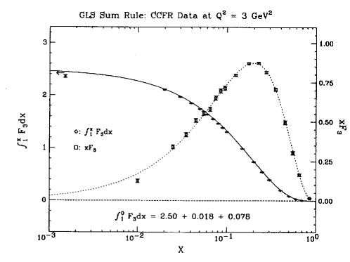
Figure 2: The Baryon sum rule from the CCFR experiment. Shown is $(xF_{3}^{ep}(x,Q^{2})+xF_{3}^{en}(x,Q^{2}))/2$ (right hand scale) and $\int_{x}^{1}dx(F_{3}^{ep}(x,Q^{2})+F_{3}^{en}(x,Q^{2}))/2$ (left scale) at $Q^{2}=3$ GeV². The curves are from a fit of the form $xF_{3}(x)=Ax^{b}(1-x)^{c}$

As well as $F_{3}$, it shows $\int_{x_{min}}^{1}dxF_{3}(x)$ as a function of $x_{min}$; the lowest value of $x$ where data are available is $x=0.015$. In performing the extrapolation to $x_{min}=0$ a form for $xF_{3}(x)$ must be assumed. A fit of the form $xF_{3}(x)=Ax^{b}(1-x)^{c}$ provides an excellent description of the data. A systematic error must be included in the quoted value of the sum rule to take into account the extrapolation to $x_{min}=0$. This systematic error is difficult to estimate, since there is no fundamental reason for preferring one extrapolation over another. Data from different values of $Q^{2}$ can only be combined if a $Q^{2}$ extrapolation is assumed. Such an extrapolation can be based on a fit to perturbative QCD. However, if this is done, a “test of QCD” from the sum rules is compromised since perturbative QCD necessarily restricts the values that the sum rules can take.

Having given these caveats, we will now discuss the current experimental values for the sum rules. For the baryon sum rule, the CCFR collaboration [131] gives,

$$S_{{\rm GLS}}=2.50\pm 0.018(stat)\pm 0.078(sys)$$ (61)

at $Q^{2}=3$ GeV². The systematic error includes the error from extrapolation into $x=0$. A more precise result has been obtained by the CCFR collaboration [132] by combining their data with that from other experiments on neutrino scattering [133, 134, 135, 136, 137]. Also, in the very large $x$ region the nucleon’s antiquark content is negligible and a relation between $F_{3}^{\nu p}$ and $F_{2}^{ep}$ exists in the Parton Model, viz  $5(F_{3}^{\nu p}(x,Q^{2})+F_{3}^{\nu n}(x,Q^{2}))=18(F_{2}^{ep}(x,Q^{2})+F_{2}^{en}(x,Q^{2}))$. The experimental precision on the baryon sum rule accuracy can therefore be improved by including data from $F_{2}^{ep(n)}$ [138] which has much higher statistics. The combined data are then extrapolated into the region below $x=0.02$ and the sum rule evaluated. Figure 3 shows the extracted value of the baryon sum rule as a function of $Q^{2}$. The curves on this figure will be discussed below.

Figure 3: The Baryon sum rule from the CCFR experiment as a function of $Q^{2}$. The inner error bar shows statistical errors and the outer a combination of statistical and systematic errors. The curves are a QCD predictions that are discussed in the text.

The solid line shows the QCD prediction including the higher twist effects, the dashed line shows the prediction of the higher twist terms are ignored. A comparison of the two curves shows that the higher twist contributions are unimportant for $Q^{2}\raisebox{-1.72218pt}{\hbox to0.0pt{$\sim$\hss}}\raisebox{1.72218pt}{$>$}5$ GeV². The QCD prediction, which corresponds to $\alpha_{s}(M_{Z})=0.12$, lies considerably below the data. The CCFR collaboration has fitted to QCD by allowing $\alpha_{s}$ to vary [132] (see also [126, 139, 140]) . The best fit corresponds to

$$\alpha_{s}(M_{Z})=0.108\pm 0.004(stat)\pm 0.004(syst)\pm 0.006(HT)$$ (62)

The data for $F_{2}^{ep}-F_{2}^{en}$ and the integral $\int_{x}^{1}(F_{2}^{ep}-F_{2}^{en})dx/x$ are shown in Figure 4 from [141]. The experiment observes no significant $Q^{2}$ variation over the range $0.5$ GeV${}^{2}<Q^{2}<10$ GeV². The measured values are extrapolated into $x=0$ assuming $F_{2}^{ep}-F_{2}^{en}=ax^{b}$. $a$ and $b$ are determined from a fit in the region $0.004<x<0.015$ to be $a=0.2\pm 0.03$, $b=0.50\pm 0.06$. This extrapolation then contributes to the quoted error. The value of the Valence Isospin sum rule is determined by the NMC [141] collaboration to be

$$S_{G}=0.235\pm 0.026$$ (63)

for $<Q^{2}>=4$ GeV². This value is shown on the figure. The same experiment has issued preliminary results from its full data set [142] which extends to smaller values of $x$ and has fitted its data together with that of BCDMS [143] and SLAC [138] to give values of $F_{2}^{ep}$ and $F_{2}^{ed}$ ($d$ represents deuterium) over the x range $0.006<x<0.9$. $Q^{2}$ corrections are applied to take higher twist effects into account and the results can then be interpreted as [144]

$$S_{G}=0.216\pm 0.027$$ (64)

for $<Q^{2}>=4$ GeV ² with no significant remaining $Q^{2}$ dependence in the range $0.5<Q^{2}<10$ GeV². Recent data from E665 [145] agree with NMC.

Figure 4: Data from the NMC collaboration on the Valence Isospin sum rule. Shown is the quantity $F_{2}^{ep}-F_{2}^{en}$ (open points, right scale) and $\int_{x}^{1}(F_{2}^{ep}-F_{2}^{en})dx/x$ (crosses, left scale). The bar at the extreme left shows the derived value of the sum rule.

The Callan-Gross relation is poorly determined. Experiments measure

$$R(x,Q^{2})=\frac{F_{2}(x,Q^{2})(1+4M^{2}x^{2}/Q^{2})-2xF_{1}(x,Q^{2})}{2xF_{1}(x,Q^{2})}$$ (65)

Data from SLAC [146, 147, 148] are shown in Figure 5.

Figure 5: The quantity $R(x,Q^{2})$ from the SLAC experiments as a function of $Q^{2}$ for certain values of $x$ at $x=0.5$ (squares), $x=0.35$ (diamonds) and $x=0.2$ (crosses).

The figure shows that $R(x,Q^{2})$ falls rapidly as $Q^{2}$ is increased and that it is small. The value is consistent with that predicted by QCD. The Isospin and Second Isospin sum rules, which are related by the Callan-Gross relation, are difficult to measure with precision as they require neutrino scattering off hydrogen and deuterium targets and the statistical errors on such measurements are poor. Data show no significant $Q^{2}$ variation in the range $2\hbox{ GeV}^{2}\raisebox{-1.72218pt}{\hbox to0.0pt{$\sim$\hss}}\raisebox{1.72218pt}{$<$}Q^{2}\raisebox{-1.72218pt}{\hbox to0.0pt{$\sim$\hss}}\raisebox{1.72218pt}{$<$}30$ GeV² and give [149]

$$S_{\rm A}=2.02\pm 0.40$$ (66)

No published results are available on the Second Isospin sum rule. However the result of Eqn. (66) together with the information on $R(x,Q^{2})$ show that the value of this rule is consistent with the expectation of $S_{{\rm Bj}}^{{\rm unpol.}}=1$.

In the case of the Spin sum rules, data are available from SMC at CERN [150, 151], using polarized muon beams scattering off deuterium and hydrogen targets, and E142 [152] and E143 [153, 154] at SLAC using polarized electron beams on He³, hydrogen and deuterium targets targets. The SLAC data only cover $x>0.03$ and $1$ GeV${}^{2}\raisebox{-1.72218pt}{\hbox to0.0pt{$\sim$\hss}}\raisebox{1.72218pt}{$<$}Q^{2}\raisebox{-1.72218pt}{\hbox to0.0pt{$\sim$\hss}}\raisebox{1.72218pt}{$<$}6.5$ GeV², while the CERN data extend to $x=0.003$ and $1$ GeV${}^{2}\raisebox{-1.72218pt}{\hbox to0.0pt{$\sim$\hss}}\raisebox{1.72218pt}{$<$}Q^{2}<\raisebox{-1.72218pt}{\hbox to0.0pt{$\sim$\hss}}\raisebox{1.72218pt}{$<$}60$ GeV². The experiments actually measure the asymmetry in scattering i.e.   the ratio of the quantity $a$ of Eqn.(4) to the unpolarized rate of Eqn.(1). No $Q^{2}$ dependence is observed in this ratio.

In order to extract $G_{1}(x,Q^{2})$ it is assumed that this ratio is independent of $Q^{2}$ and therefore that the $Q^{2}$ dependence of $G_{1}(x,Q^{2})$ is given by that of $F_{1}(x,Q^{2})$ and $F_{2}(x,Q^{2})$. $G_{1}(x,Q^{2})$ is then extrapolated to $Q^{2}=5$ GeV². Data are extrapolated to $x=0$ using the assumption that $G_{1}(x,Q^{2})\sim x^{\alpha}$ with $0<\alpha<0.5$. An extrapolation in the region $0.6<x<1$ is also needed, but this introduces a very small error since $G_{1}(x,Q^{2})$ is very small in this region. The contribution of the structure function $G_{2}(x,Q^{2})$ is suppressed by the $1/Q^{2}$ term in Eqn.(4) and no information about it can be extracted from the data.

These extrapolations enable the Spin sum rules for $G_{1}(x,Q^{2})$ to be evaluated. The SMC data alone [150, 151, 155] give for the Polarized Isospin sum rule

$$S_{{\rm Bj}}=0.199\pm 0.038$$ (67)

at $Q^{2}=10.4$ GeV², whereas at $Q^{2}$=3 $GeV^{2}$, the SLAC data [152, 153, 154] give

$$S_{{\rm Bj}}=0.149\pm 0.014$$ (68)

The different form used for the extrapolation to smaller values of $x$ is partly responsible for the smaller values. The experiments can be combined with earlier results involving hydrogen targets [156, 157] to give, at $Q^{2}=5$ GeV², [158]

$$\begin{array}[]{rl}S_{{\rm EJ}}^{p}=&0.136\pm 0.010\cr S_{{\rm EJ}}^{n}=&-0.067\pm 0.016.\end{array}$$ (69)

The Polarized Isospin sum rule determined from these is

$$S_{{\rm Bj}}=0.203\pm 0.023$$ (70)

3.2 Theory vs. Experiment

Table 2 shows a comparison of the experimental values discussed above with theoretical predictions from Table 1. In the cases where the experiments have corrected for the effects of higher twist the relevant comparison is with the highest order perturbative QCD result available and it is this number that is given in the theory column. No entries are shown for the $G_{2}$ and Second Isospin sum rules where no data exist.

	$\displaystyle\frac{Q^{2}}{{\rm GeV}^{2}}$	theory	Expt.
$S_{{\rm G}}$	4	0.335	0.216$\pm$0.027
$S_{{\rm GLS}}$	3	2.388	2.50 $\pm$ 0.08
$S_{{\rm A}}$	3	2	2.02$\pm$ 0.40
$S_{{\rm Bj}}$	5	0.178	0.203$\pm$ 0.023
$S_{{\rm EJ}}^{p}$	5	0.171	0.136$\pm$ 0.010
$S_{{\rm EJ}}^{n}$	5	-0.0135	-0.067 $\pm$ 0.016

Table 2: Comparison of the theoretical and experimental values of the sum rules.

It can be seen from the Table that the sum rules fall into three categories. First, the Isospin sum rule has very large experimental uncertainties but the measured values are consistent with the expectations of QCD. Second, the Baryon sum rule and Polarized Isospin sum rule are compatible with QCD, but have experimental errors that are small enough so that the measurements can discriminate between the QCD results at different orders in perturbation theory. In these cases the data are consistent with the QCD expectations and are inconsistent with the Naive Parton Model. Finally, the Spin and Valence Isospin sum rules have experimental values that are inconsistent with the Naive Parton Model or QCD predictions.

The second category can be used to measure the strong coupling constant $\alpha_{s}$. Figure 3 shows the $Q^{2}$ dependence of the Baryon sum rule. This value is somewhat lower than the world average [159] The quoted error is dominated by that due to the Higher Twist terms ($HT$). The Polarized Isospin sum rule has also been used to determine $\alpha_{s}$ [160]:-

$$\alpha_{s}(M_{Z})=0.122^{+0.005}_{-0.009}$$ (71)

if the higher twist terms are neglected. or

$$\alpha_{s}(M_{Z})=0.118^{+0.007}_{-0.014}$$ (72)

if they are included.

The final category needs more discussion. The Valence Isospin sum rule discrepancy between theory and experiment shown in table 2 can be removed by dropping the assumption that $\int_{0}^{1}dx(\overline{u}(x)-\overline{d}(x))=0$. Using the Naive Parton Model (see Eqn. 14) and the data we obtain

$$\int_{0}^{1}dx(\overline{u}(x)-\overline{d}(x))=-0.176\pm 0.040.$$ (73)

The QCD corrections are much smaller than the error on this result. Additional experimental information is available from the processes $pd\to\mu^{+}\mu^{-}+anything$ and $pp\to\mu^{+}\mu^{-}+anything$ which, in the Parton Model, are due to quark antiquark annihilation. Data from NA51 [161] indicate that $\overline{u}(x)/\overline{d}(x)=0.51\pm 0.08$ at $x=0.18$ and $Q^{2}=2.5$ GeV². The possible non-equality of $\overline{u}(x)$ and $\overline{d}(x)$ was first suggested in [162] where a possible parameterization was introduced. Several authors have attempted to estimate the size of $\overline{u}(x)-\overline{d}(x)$ that could arise from non-perturbative effects. Some have attempted to explain the effect in terms of a pion cloud surrounding the nucleon [163]. Other models are based a chiral Lagrangian [164] approach that starts with a nucleon consisting of three valence quarks then generates the anti-quark distributions from pions emitted in processes like $u\to d\pi^{+}$ [165, 166]. Models of this type produce a difference $(\overline{u}(x)-\overline{d}(x))$ that is concentrated at very small values of $x$ and the ratio $\overline{u}(x)/\overline{d}(x)$ is predicted to be quite small.

The predictions for the values of the Spin sum rules depend upon the assumed values for $a_{0}$, $a_{3}$ and $a_{8}$. There is no fundamental reason for the first of these to take the value $a_{0}=\sqrt{3}a_{8}$ which was the original assumption of [23] and is the value used in the table. If we use $a_{0}=0.12\pm 0.027$, obtained from the value of $\Delta S$ obtained from $\nu p$ elastic scattering [14] we have at $Q^{2}=5$ GeV² the “predictions” $S_{{\rm EJ}}^{n}=-0.065\pm 0.030$ and $S_{{\rm EJ}}^{p}=0.12\pm 0.03$ both of which agree with the experimental results shown in Table 2. Instead we can use the experimental results for $S_{EJ}^{p}$ and $S_{EJ}^{n}$ to determine $a_{0}$ from the QCD forms of Eqn.(42) together with the higher twist corrections. This gives $a_{0}=0.19\pm 0.07$. Using the Naive Parton Model relation of Eqn.(LABEL:a0eq) implies that $\int dx(\Delta s(x)+\Delta\overline{s}(x))=-0.13\pm 0.03$ from whence we can also infer that $\int dx(\Delta u(x)+\Delta\overline{u}(x))=0.8$ and $\int dx(\Delta d(x)+\Delta\overline{d}(x))=0.4$. Everything is consistent but one is left with the annoying question of what is carrying most of the nucleon’s spin. In the model where the nucleon is viewed a soliton-like solution of [167] one expects $a_{0}=0$ [168] in the limit of zero quark mass and large number of colors. In this interpretation all of the nucleon’s spin is carried by orbital angular momentum. Reference [169] can be consulted for a detailed review.

If the gluon distribution in the proton is polarized, there is an additional complication. The scattering process $e+g\to eq\overline{q}$ can generate a contribution to $G_{1}(x,Q^{2})$ at order $\alpha_{s}$. Adding this term to the Naive Parton Model result is equivalent to replacing Eqn.(LABEL:a0eq) by [170]

$$a_{0}=\int_{0}^{1}dx\Big{(}\Delta u+\Delta\bar{u}+\Delta d+\Delta\bar{d}+\Delta s+\Delta\bar{s}-n_{f}\frac{\alpha_{s}}{2\pi}\Delta g\Big{)}$$ (74)

This contribution is not present in the Operator Product analysis presented above. It can be introduced if one observes that while the operator corresponding to the singlet axial current is not conserved and is therefore subject to renormalization due to the axial anomaly [171, 172, 173], a linear combination of this operator and a gauge variant operator made up of gluon fields is not renormalized. If this term is included the form of the QCD corrections given in Eqn.(42) are the same except that $a_{0}^{{\rm inv}}$ is interpreted as that of Eqn.(74). The data are now to be interpreted as implying $\int dx(\Delta s+\Delta\bar{s}-n_{f}\frac{\alpha_{s}}{2\pi}\Delta g=-0.13\pm 0.03$. If we assume that $\Delta S=0$ then $\int dx\Delta g=3.2\pm 0.75$ at $Q^{2}=5$ GeV². This substantial polarization should be observable in other experiments. For example, the production of pions at large transverse momentum in proton-proton scattering proceeds via parton parton scattering of the type $q+g\to gq$. If both protons are polarized an asymmetry

$$A_{LL}=\frac{d\sigma(++)-d\sigma(-+)}{d\sigma(++)+d\sigma(-+)}$$ (75)

can be formed (the $\pm$ arguments refer the helicity of the incident protons) which is depends upon $\Delta g(z)$. An experiment at FermiLab [174] observes an asymmetry that is consistent with zero for transverse momenta of pions less than 3 GeV. More recently [175] the same experiment has measured the asymmetry for double $\pi^{0}$ production. Again the asymmetry is consistent with zero. If models for $\Delta q$ are assumed [176] then a constraint can be obtained on $\Delta g$. This constraint is sufficient to rule out some models [177], but others that have $\int dx\Delta g(x)\sim 5$ [178] are not excluded.

4 Conclusions

The Parton Model sum rules represent fundamental predictions of QCD. The experimental precision of many of these rules is such that consistency with the theory can be established. In the case of a few of the rules, notably the baryon sum rule, the data are sufficiently precise that consistency can be checked in detail and a value of the strong coupling constant obtained whose error is competitive with the best measurements [159]. In this case the theoretical errors coming from the poor knowledge of higher twist terms and the order $\alpha_{s}^{4}$ terms contribute significantly to the error on $\alpha_{s}$. Improvement in these areas is unlikely to appear in the near future. The failure of the Valence Isospin sum rule has led to the realization that $\overline{u}(x)\neq\overline{d}(x)$ and while there is some theoretical understanding of how this might arise, the difference, like all other structure functions, must be extracted from data. The failure of the naive form of the Spin sum rules has led to an interesting situation. There must be significant polarization in the strange quarks and/or the gluons. More accurate data on $\nu p$ elastic scattering might enable the former to be constrained. The latter should be constrained when polarized proton-proton scattering experiments become available at RICH in the next few years [179]

The advent of data from HERA[180] have enabled structure functions to be measured at smaller values of $x$ than those in fixed target experiments. Nevertheless, the statistical errors on these data are still quite large and they are, of course, only available for $F_{2}^{ep}(x,Q^{2})$. In the future, data from polarized $ep$ scattering will be available from this facility [181] that will considerably extend the range of $x$ and $Q^{2}$ available for the measurements of $G_{1}(x,Q^{2})$ and reduce the error on the Spin sum rules resulting from the extrapolation into $x=0$.

Acknowledgments
This work was supported by the Director, Office of Energy Research, Office of High Energy and Nuclear Physics, Division of High Energy Physics of the U.S. Department of Energy under Contract DE-AC03-76SF00098 and (AK) by Deutsche Forschungsgemeinschaft (DFG) under grant number Kw 8/1-1. Accordingly, the U.S. Government retains a nonexclusive, royalty-free license to publish or reproduce the published form of this contribution, or allow others to do so, for U.S. Government purposes.

Appendix

The effective coupling constant in next-next-to-leading order may be written in the form

$$\begin{array}[]{ll}\displaystyle\frac{\bar{\alpha}_{s}}{\pi}=&\displaystyle\frac{1}{\beta_{0}L}\Bigg{[}1-\frac{1}{\beta_{0}L}\frac{\beta_{1}\ln L}{\beta_{0}}\\ &\displaystyle+\frac{1}{\beta_{0}^{2}L^{2}}\left(\frac{\beta_{1}^{2}}{\beta_{0}^{2}}(\ln^{2}L-\ln L-1)+\frac{\beta_{2}}{\beta_{0}}\right)\Bigg{]}\end{array}$$ (76)

where $L\equiv\ln(Q^{2}/\Lambda^{2})$ and $\bar{\alpha}_{s}(Q^{2}=\mu^{2})=\alpha_{s}(\mu^{2})$. The coefficients of the beta-function are known up to the three loop level [3, 4, 182, 183, 184, 185]:

$$\begin{array}[]{l}\displaystyle\beta_{0}=\frac{1}{4}\left(11-\frac{2}{3}n_{f}\right),\;\;\;\beta_{1}=\frac{1}{16}\left(102-\frac{38}{3}n_{f}\right),\\ \displaystyle\beta_{2}=\frac{1}{64}\left(\frac{2857}{2}-\frac{5033}{18}n_{f}+\frac{325}{54}n_{f}^{2}\right)\end{array}$$ (77)

Anomalous dimensions of singlet and nonsinglet operators were calculated in a number of works for both unpolarized [59, 60, 27, 61, 62], [39, 63, 64, 65, 66, 67] and polarized scattering [51, 52, 27, 53, 34, 54, 55, 56]. Some of the results are given here. The coefficients of the nonsinglet anomalous dimension for unpolarized scattering read

$$\begin{array}[]{l}\displaystyle\gamma_{n=1}^{{\rm NS}(0)}=-\frac{1}{4}C_{F}\left[1-\frac{2}{n(n+1)}+4\sum_{j=2}^{n}\frac{1}{j}\right]_{n=1}=0\\ \displaystyle\gamma_{n=1}^{{\rm NS}(1)+}=-\frac{1}{36}\left(13+8\zeta(3)-2\pi^{2}\right)\\ \displaystyle\gamma_{n=1}^{{\rm NS}(1)-}=0.\end{array}$$ (78)

For polarized scattering one has the following nonsinglet anomalous dimensions $\Delta\gamma_{n}^{{\rm NS}(0)}=\gamma_{n}^{{\rm NS}(0)}$ and $\Delta\gamma_{n}^{{\rm NS}(1)\pm}=\gamma_{n}^{{\rm NS}(1)\pm}$. Finally the coefficients for the singlet quark diagonal anomalous dimension matrix elements are

$$\begin{array}[]{ll}\displaystyle\Delta\gamma_{n,qq}^{{\rm S}(0)}&\displaystyle=\gamma_{n}^{{\rm NS}(0)}\\ \displaystyle\Delta\gamma_{n=1,qq}^{{\rm S}(1)}=&\displaystyle\frac{1}{16}\left[\gamma_{n}^{{\rm NS}(1)-}-4C_{F}n_{f}\frac{n^{4}+2n^{3}+2n^{2}+5n+2}{n^{3}(1+n)^{3}}\right]_{n=1}\\ &\displaystyle=-\frac{1}{2}n_{f}\\ \displaystyle\Delta\gamma_{n=1,qq}^{{\rm S}(2)}=&\displaystyle\frac{1}{64}\left(\left[18C_{F}^{2}-\frac{142}{3}C_{F}C_{A}\right]n_{f}+\frac{4}{3}C_{F}n_{f}^{2}\right)\\ &\displaystyle=-\frac{59}{24}n_{f}+\frac{1}{36}n_{f}^{2}\end{array}$$ (79)

Finally we give the analytic formulae of the coefficient functions corresponding to the first moments of the various structure functions. The nonsinglet coefficient function for the structure function $F_{2}$ of unpolarized electron nucleon scattering is given in the $\overline{\mbox{MS}}$ scheme [69, 62] by

$$\begin{array}[]{l}\displaystyle C^{(ep-en)}_{F_{2},n=1}(1,\bar{A}(Q^{2}))=1+\left(\frac{\alpha_{s}}{\pi}\right)\Bigg{[}\frac{C_{f}}{4}\Bigg{(}-9+\frac{2}{n^{2}}+\frac{4}{(n+1)}+\frac{3}{n}\\ \hphantom{xxx}\displaystyle+3\sum_{j=1}^{n}\frac{1}{j}-4\sum_{j=1}^{n}\frac{1}{j^{2}}-\frac{2}{n(n+1)}\sum_{j=1}^{n}\frac{1}{j}+4\sum_{s=1}^{n}\frac{1}{s}\sum_{j=1}^{s}\frac{1}{j}\Bigg{)}\\ \hphantom{xxx}\displaystyle-\gamma^{{\rm NS}(0)}_{n}(\ln(4\pi)-\gamma_{E})\Bigg{]}_{n=1}=1\end{array}$$ (80)

The nonsinglet [79, 80, 81, 82, 34] and the singlet [53, 34, 83] coefficient functions for polarized electron-nucleon scattering read

$$\begin{array}[]{l}\displaystyle C^{{\rm NS}}_{G_{1},n=1}\left(1,\bar{A}(Q^{2})\right)=1-\frac{3}{4}C_{F}\frac{\bar{\alpha}_{s}}{\pi}\\ \hphantom{xxx}\displaystyle+\left(\frac{\bar{\alpha}_{s}}{\pi}\right)^{2}C_{F}\left[\frac{21}{32}C_{F}-\frac{23}{16}C_{A}+\frac{1}{4}n_{f}\right]\\ \hphantom{xxx}\displaystyle+\left(\frac{\bar{\alpha}_{s}}{\pi}\right)^{3}\left[-\frac{3}{128}C_{F}^{3}+C_{F}^{2}C_{A}\left(\frac{1241}{576}-\frac{11}{12}\zeta(3)\right)\right.\\ \hphantom{xxx}\displaystyle\hphantom{\left(\frac{\bar{\alpha}_{s}}{\pi}\right)^{3}[}+C_{F}C_{A}^{2}\left(-\frac{5437}{864}+\frac{55}{24}\zeta(5)\right)\\ \hphantom{xxx}\displaystyle\hphantom{\left(\frac{\bar{\alpha}_{s}}{\pi}\right)^{3}[}+C_{F}^{2}n_{f}\left(-\frac{133}{1152}-\frac{5}{24}\zeta(3)\right)\\ \hphantom{xxx}\displaystyle\hphantom{\left(\frac{\bar{\alpha}_{s}}{\pi}\right)^{3}[}+C_{F}C_{A}n_{f}\left(\frac{3535}{1728}+\frac{3}{8}\zeta(3)-\frac{5}{12}\zeta(5)\right)\\ \hphantom{xxx}\displaystyle\hphantom{\left(\frac{\bar{\alpha}_{s}}{\pi}\right)^{3}[}\left.-\frac{115}{864}C_{F}n_{f}^{2}\right]\\ \hphantom{xxx}\displaystyle=1-\frac{\bar{\alpha}_{s}}{\pi}+\left(\frac{\bar{\alpha}_{s}}{\pi}\right)^{2}\left[-\frac{55}{12}+\frac{1}{3}n_{f}\right]\\ \hphantom{xxx}\displaystyle+\left(\frac{\bar{\alpha}_{s}}{\pi}\right)^{3}\left[-\frac{13841}{216}-\frac{44}{9}\zeta(3)+\frac{55}{2}\zeta(5)\right.\\ \hphantom{xxx}\displaystyle\hphantom{+\left(\frac{\bar{\alpha}_{s}}{\pi}\right)^{3}[}+n_{f}\left(\frac{10339}{1296}+\frac{61}{54}\zeta(3)-\frac{5}{3}\zeta(5)\right)\\ \hphantom{xxx}\displaystyle\hphantom{+\left(\frac{\bar{\alpha}_{s}}{\pi}\right)^{3}[}\left.-\frac{115}{648}n_{f}^{2}\right]\end{array}$$ (81)

$$\begin{array}[]{l}\displaystyle C^{{\rm S}}_{G_{1},n=1}\left(1,\bar{A}(Q^{2})\right)=1-\frac{3}{4}\frac{\bar{\alpha}_{s}}{\pi}\\ \hphantom{xxx}\displaystyle+\left(\frac{\bar{\alpha}_{s}}{\pi}\right)^{2}\left[\frac{21}{32}C_{F}^{2}-\frac{23}{16}C_{F}C_{A}+C_{F}n_{f}\left(\frac{13}{48}+\frac{1}{2}\zeta(3)\right)\right]\\ \hphantom{xxx}=\displaystyle 1-\frac{\bar{\alpha}_{s}}{\pi}+\left(\frac{\bar{\alpha}_{s}}{\pi}\right)^{2}\left[-\frac{55}{12}+n_{f}\left(\frac{13}{36}+\frac{2}{3}\zeta(3)\right)\right]\end{array}$$ (82)

The coefficient function for the neutrino structure function $F_{3}$ has the following form [69, 82, 33, 34]:

$$\begin{array}[]{l}\displaystyle C^{(\nu{\cal N})}_{F_{3},n=1}\left(1,\bar{A}(Q^{2})\right)=1-\frac{3}{4}C_{F}\frac{\bar{\alpha}_{s}}{\pi}\\ \hphantom{xxx}\displaystyle+\left(\frac{\bar{\alpha}_{s}}{\pi}\right)^{2}C_{F}\left[\frac{21}{32}C_{F}-\frac{23}{16}C_{A}+\frac{1}{4}n_{f}\right]\\ \hphantom{xxx}\displaystyle+\left(\frac{\bar{\alpha}_{s}}{\pi}\right)^{3}\left[-\frac{3}{128}C_{F}^{3}+C_{F}^{2}C_{A}\left(\frac{1241}{576}-\frac{11}{12}\zeta(3)\right)\right.\\ \hphantom{xxx}\displaystyle\hphantom{\left(\frac{\bar{\alpha}_{s}}{\pi}\right)^{3}[}+C_{F}C_{A}^{2}\left(-\frac{5437}{864}+\frac{55}{24}\zeta(5)\right)\\ \hphantom{xxx}\displaystyle\hphantom{\left(\frac{\bar{\alpha}_{s}}{\pi}\right)^{3}[}+C_{F}^{2}n_{f}\left(-\frac{133}{1152}-\frac{5}{24}\zeta(3)\right)\\ \hphantom{xxx}\displaystyle\hphantom{\left(\frac{\bar{\alpha}_{s}}{\pi}\right)^{3}[}+C_{F}C_{A}n_{f}\left(\frac{3535}{1728}+\frac{3}{8}\zeta(3)-\frac{5}{12}\zeta(5)\right)\\ \hphantom{xxx}\displaystyle\hphantom{\left(\frac{\bar{\alpha}_{s}}{\pi}\right)^{3}[}-\frac{115}{864}C_{F}n_{f}^{2}\\ \hphantom{xxx}\displaystyle\hphantom{\left(\frac{\bar{\alpha}_{s}}{\pi}\right)^{3}[}\left.+n_{f}\frac{d^{abc}d^{abc}}{N_{C}}\left(-\frac{11}{192}+\frac{1}{8}\zeta(3)\right)\right]\end{array}$$ (83)

$$\begin{array}[]{ll}\displaystyle=&\displaystyle 1-\frac{\bar{\alpha}_{s}}{\pi}+\left(\frac{\bar{\alpha}_{s}}{\pi}\right)^{2}\left[-\frac{55}{12}+\frac{1}{3}n_{f}\right]\\ &\displaystyle+\left(\frac{\bar{\alpha}_{s}}{\pi}\right)^{3}\left[-\frac{13841}{216}-\frac{44}{9}\zeta(3)+\frac{55}{2}\zeta(5)\right.\\ &\displaystyle\hphantom{+\left(\frac{\bar{\alpha}_{s}}{\pi}\right)^{3}[}+n_{f}\left(\frac{10009}{1296}+\frac{91}{54}\zeta(3)-\frac{5}{3}\zeta(5)\right)\\ &\displaystyle\hphantom{+\left(\frac{\bar{\alpha}_{s}}{\pi}\right)^{3}[}\left.-\frac{115}{648}n_{f}^{2}\right]\end{array}$$ (84)

The coefficient function for the nonsinglet structure function $F_{1}$ of neutrino and antineutrino scattering reads [69, 89, 90]

$$\begin{array}[]{l}\displaystyle C^{(\nu n-\nu p)}_{F_{1},n=1}(1,\bar{A}(Q^{2}))=1-\frac{1}{2}C_{F}\frac{\bar{\alpha}_{s}}{\pi}\\ \hphantom{xxx}\displaystyle+\left(\frac{\bar{\alpha}_{s}}{\pi}\right)^{2}C_{F}\left[\frac{11}{16}C_{F}-\frac{91}{72}C_{A}+\frac{2}{9}n_{f}\right]\\ \hphantom{xxx}\displaystyle+\left(\frac{\bar{\alpha}_{s}}{\pi}\right)^{3}\left[C_{F}^{3}\left(-\frac{313}{64}-\frac{47}{4}\zeta(3)+\frac{35}{2}\zeta(5)\right)\right.\\ \hphantom{xxx}\displaystyle\hphantom{\left(\frac{\bar{\alpha}_{s}}{\pi}\right)^{3}[}+C_{F}^{2}C_{A}\left(\frac{2731}{288}+\frac{91}{6}\zeta(3)-\frac{95}{4}\zeta(5)\right)\\ \hphantom{xxx}\displaystyle\hphantom{\left(\frac{\bar{\alpha}_{s}}{\pi}\right)^{3}[}+C_{F}C_{A}^{2}\left(-\frac{8285}{1296}-\frac{5}{2}\zeta(3)+5\zeta(5)\right)\\ \hphantom{xxx}\displaystyle\hphantom{\left(\frac{\bar{\alpha}_{s}}{\pi}\right)^{3}[}+C_{F}^{2}n_{f}\left(-\frac{335}{576}+\frac{1}{12}\zeta(3)\right)\\ \hphantom{xxx}\displaystyle\hphantom{\left(\frac{\bar{\alpha}_{s}}{\pi}\right)^{3}[}+C_{F}C_{A}n_{f}\left(\frac{4235}{2592}-\frac{7}{12}\zeta(3)+\frac{5}{6}\zeta(5)\right)\\ \hphantom{xxx}\displaystyle\hphantom{\left(\frac{\bar{\alpha}_{s}}{\pi}\right)^{3}[}\left.-\frac{155}{1296}C_{F}n_{f}^{2}\right]\end{array}$$ (85)

$$\begin{array}[]{ll}\displaystyle=&\displaystyle 1-\frac{2}{3}\frac{\bar{\alpha}_{s}}{\pi}+\left(\frac{\bar{\alpha}_{s}}{\pi}\right)^{2}\left[-\frac{23}{6}+\frac{8}{27}n_{f}\right]\\ &\displaystyle+\left(\frac{\bar{\alpha}_{s}}{\pi}\right)^{2}\left[-\frac{4075}{108}+\frac{622}{27}\zeta(3)-\frac{680}{27}\zeta(5)\right.\\ &\displaystyle+n_{f}\left(\frac{3565}{648}-\frac{59}{27}\zeta(3)+\frac{10}{3}\zeta(5)\right)\left.-\frac{155}{972}n_{f}^{2}\right]\end{array}$$ (86)

References

- [1] Bjorken JD, Paschos E. Phys. Rev. 185:1975 (1969).
- [2] Feynman RP. Phys. Rev. Lett. 12:1415 (1969).
- [3] Politzer HD. Phys. Rev. Lett. 30:1346 (1973).
- [4] Gross DJ, Wilczek FW. Phys. Rev. Lett. 30:1343 (1973).
- [5] Altarelli G. Phys. Rept. 81:1 (1982).
- [6] Reya E. Phys. Rept. 69:195 (1981).
- [7] Buras A. Rev. Mod. Phys. 52:199 (1980).
- [8] For a summary see Manohar A. in Review of Particle Properties Phys. Rev. 1996 (to appear).
- [9] Callan C, Gross DJ. Phys. Rev. Lett. 22:156 (1969).
- [10] Kobayashi M, Maskawa T. Prog. Theor. Phys. 49:652 (1973).
- [11] Review of Particle Properties Phys. Rev. 1996 (to appear).
- [12] Close F, Roberts RG. Phys. Lett. B316:165 (1993).
- [13] Ahrens LA, et al. Phys.Rev. D35:785 (1987).
- [14] Kaplan DB, Manohar A. Nucl. Phys. B310:527 (1988).
- [15] Ellis J, Karliner M. Phys. Lett. B213:73 (1988).
- [16] Alberico WM, et al. hep-ph/9508277 (1995).
- [17] Gross DJ, Llewellyn Smith CH. Nucl. Phys. B 14:337 (1969).
- [18] Adler S. Phys. Rev. 143:1144 (1966).
- [19] Gottfried K. Phys. Rev. Lett. 18:1174 (1967).
- [20] Bjorken JD. Phys. Rev. 163:1767 (1967).
- [21] Bjorken JD. Phys. Rev 148:1467 (1966), Phys. Rev D 1:1376 (1970),
- [22] Gourdin M. Nucl. Phys. 38:418 (1972).
- [23] Ellis J, Jaffe RL. Phys. Rev D 9:1444 (1974), (E) Phys. Rev D 10:1669 (1974).
- [24] Burkhard H, Cottingham WN. Ann. of Phys. 56:453 (1970).
- [25] Collins JC, Soper DE, Sterman G. in Perturbative Quantum Chromodynamics, edited by A. H. Mueller (World Scientific Singapore), p. 1.
- [26] Sterman G. et al. Rev. Mod. Phys., 67:157 (1995).
- [27] Altarelli G, Parisi G. Nucl. Phys. B 126:298 (1977).
- [28] Altarelli G, Ellis RK, Martinelli G. Nucl. Phys. B 143:521 (1978), (E) Nucl. Phys. B 146:544 (1978).
- [29] Humpert B, van Neerven WL. Nucl. Phys. B 184:225 (1981).
- [30] van Neerven WL, Zijlstra EB. Phys. Lett. B 272:127 (1991).
- [31] Zijlstra EB, van Neerven WL. Phys. Lett. B 273:476 (1991).
- [32] Zijlstra EB, van Neerven WL. Nucl. Phys. B 383:525 (1992).
- [33] Zijlstra EB, van Neerven WL. Phys. Lett. B 297:377 (1992).
- [34] Zijlstra EB, van Neerven WL. Nucl. Phys. B 417:61 (1994), (E) Nucl. Phys. B 426:245 (1994).
- [35] Gribov VN, Lipatov LN. Sov. J. Nucl. Phys. 15:438 (1972); Dokshitzer YuL. Sov. Phys. JETP 46:461 (1977).
- [36] Floratos EG, Kounnas C, Lacaze R. Phys. Lett. B 98:89 (1981).
- [37] Floratos EG, Kounnas C, Lacaze R. Phys. Lett. B 98:285 (1981).
- [38] Floratos EG, Kounnas C, Lacaze R. Nucl. Phys. B 192:417 (1981).
- [39] Curci G, Furmanski W, Petronzio R. Nucl. Phys. B 175:27 (1980).
- [40] Furmanski W, Petronzio R. Phys. Lett. B 97:437 (1980).
- [41] Furmanski W, Petronzio R. Z. Phys. C 11:293 (1982).
- [42] Lopez, C Yndurain, FJ, Nucl. Phys. B183:157 (1981).
- [43] Vogelsang V. RAL-TR-95-071 (1995).
- [44] Vogelsang V. RAL-TR-96-026 (1996).
- [45] Ellis RK, Vogelsang V. CERN-TH-96-50 (1996)
- [46] Wilson K. Phys. Rev. 179:1499 (1969).
- [47] Christ N, Hasslacher B, Mueller A. Phys. Rev. D 6:3543 (1972).
- [48] Stuckelberg, ECG Petermann,A. Helv. Phys. Acta. 26:499 (1953); Gell-Mann,M Low, F Phys. Rev. 95:1300 (1954).
- [49] Adler SL. Phys. Rev. 177:2426 (1969).
- [50] Bell JS, Jackiw R. Nuov. Cim. 60 A:47 (1969).
- [51] Ahmed MA, Ross GG. Phys. Lett. 56B:385 (1975); Nucl. Phys. B 111:441 (1976).
- [52] Sasaki K. Prog. Theor. Phys 54:1816 (1975).
- [53] Kodaira J. Nucl. Phys. B 165:129 (1980).
- [54] Mertig R, van Neerven WL. INLO-PUB-6/95, NIKHEF-H/95-031, (HEP-PH/9506451).
- [55] Larin SA. Phys. Lett. B 303:113 (1993).
- [56] Chetyrkin KG, Kühn JH. Z. Phys. C 60:497 (1993).
- [57] ’t Hooft G. Nucl. Phys. 61B:455 (1973).
- [58] Caswell W, Wilczek F. Phys. Lett. B 49:291 (1974).
- [59] Georgi H, Politzer HD. Phys. Rev. D 9:416 (1974).
- [60] Gross DJ, Wilczek F. Phys. Rev. D 8:3633 (1973); Phys. Rev. D 9:980 (1974).
- [61] Floratos EG, Ross DA, Sachrajda CT. Nucl. Phys. B 129:66 (1977), (E) Nucl. Phys. B 139:545 (1979).
- [62] Floratos EG, Ross DA, Sachrajda CT. Phys. Lett. 80B:269 (1979), (E) Phys. Lett. 87B:403 (1979), Nucl. Phys. B 152:493 (1979).
- [63] Hamberg R, van Neerven WL. Nucl. Phys. B 379:143 (1992).
- [64] Gonzáles-Arroyo A, López C, Ynduráin FJ. Nucl. Phys. B 153:161 (1979).
- [65] Gonzáles-Arroyo A, López C. Nucl. Phys. B 166:429 (1980).
- [66] Larin SA, Tkachov FV, Vermaseren JAM. Phys. Lett. B 272:121 (1991).
- [67] Larin SA, van Ritbergen T, Vermaseren JAM. Nucl. Phys. B 427:41 (1994).
- [68] Glück M, Reya E, Stratmann M. HEP-PH/9508347.
- [69] Bardeen WA, Buras AJ, Duke DW, Muta T. Phys. Rev. D 18:3998 (1978).
- [70] Altarelli G, Ellis RK, Martinelli G. Nucl. Phys. B 157:461 (1979).
- [71] Harada K, Kaneko T, Sakai N. Nucl. Phys. B 155:169 (1979).
- [72] Zee A, Wilczek F, Treimann SB. Phys. Rev. D 10:2881 (1974).
- [73] Hinchliffe I, Llewellyn Smith CH. Nucl. Phys B 128:93 (1977).
- [74] de Rújula A, Georgi H, Politzer HD. Ann. of Phys. 103:315 (1977).
- [75] Calvo M. Phys. Rev. D 15:730 (1977).
- [76] Abad J, Humpert B. Phys. Lett. 78B:627 (1978).
- [77] Ross DA, Sachradja CT. Nucl. Phys. B149:497 (1978).
- [78] Kubar-André J, Paige FE. Phys. Rev. D 19:221 (1979).
- [79] Kodaira J, Matsuda S, Muta T, Sasaki K, Uematsu T. Phys. Rev. D20:627 (1979); Kodaira J, Matsuda S, Sasaki K, Uematsu T. Nucl. Phys. B 159:99 (1979).
- [80] Gorishny SG, Larin SA. Phys. Lett. B 172:109 (1986).
- [81] Gorishny SG, Larin SA. Nucl. Phys. B 283:452 (1987).
- [82] Larin SA, Vermaseren JAM. Phys. Lett. B 259:345 (1991).
- [83] Larin SA. Phys. Lett. B 334:192 (1994).
- [84] Jaffe RL. Comm. Nucl. Part. Phys. 19:239 (1990).
- [85] Anselmino M, Efremov A, Leader E. Phys. Rept. 261:1 (1995).
- [86] Altarelli G, Lampe B, Nason P, Ridolfi G.Phys. Lett. B 334:187 (1994).
- [87] Kodaira J, Matsuda S, Uematsu T. Phys. Lett. B 345:527 (1995).
- [88] Mertig R, van Neerven WL. Z. Phys. C 60:489 (1993), (E) Z. Phys. C 65:360 (1995).
- [89] Chetyrkin KG, Gorishny SG, Larin SA, Tkachov FV. Phys. Lett. 137B:230 (1984).
- [90] Larin SA, Tkachov FV, Vermaseren JAM. Phys. Rev. Lett. 66:862 (1991).
- [91] Nanopoulos D, Ross GG. Phys. Lett. 58B:105 (1975).
- [92] Herrero MJ, Miramontes JL. Phys. Rev. D 34:138 (1986) .
- [93] Miramontes JL, Sanchez Guillén J, Zas E. Phys. Rev. D 35:863 (1987).
- [94] Kazakov DI, et al. Phys. Rev. Lett. 65:1535 (1990), (E) Phys. Rev. Lett. 65:2921 (1990).
- [95] Sanchez Guillén J, et al. Nucl. Phys. B 353:337 (1991).
- [96] Duke DW, Kimel JD, Sowell GA. Phys. Rev. D 25:71 (1982)
- [97] Coulson SN, Ecclestone RE. Phys. Lett. B 115:415 (1982); Nucl. Phys. B 211:317 (1983).
- [98] Devoto A, Duke DW, Kimel JD, Sowell GA. Phys. Rev. D 30:541 (1984).
- [99] Kazakov DI, Kotikov AB. Nucl. Phys. B 307:721 (1988); Phys. Lett. B 291: 171 (1992).
- [100] Larin SA, Vermaseren JAM. Z. Phys. C 57:93 (1993).
- [101] Kataev AL, Starshenko VV. Mod. Phys. Lett. A 10:235 (1995).
- [102] Samuel MA, Li G, Steinfelds E. Phys. Lett. B 323:188 (1994).
- [103] Kataev AL. Phys. Rev. D50:R5469 (1994).
- [104] Nachtmann O. Nucl. Phys.B 63:237 (1973) .
- [105] Shuryak EV, Vainshtein AI. Nucl. Phys. B 199:451 (1982).
- [106] Shuryak EV, Vainshtein AI. Nucl. Phys. B 201:142 (1982).
- [107] Shifman MA, Vainshtein AI, Zakharov VI. Nucl. Phys. B 147:385,448,519 (1979).
- [108] Balitsky II, Braun VM, Kolesnichenko AV. Phys. Lett. B 242:245 (1990), (E) Phys. Lett. B 318:648 (1993).
- [109] Ji X, Unrau P. Phys. Lett. B 333:228 (1994).
- [110] Stein E, Górnicki G, Mankiewicz L, Schäfer A, Greiner W. Phys. Lett. B 343:369 (1995).
- [111] Stein E, Górnicki G, Mankiewicz L, Schäfer A. Phys. Lett. B 353:107 (1995).
- [112] Anselmino M, Ioffe BL, Leader E. Sov. J. Nucl. Phys. 49:136 (1989).
- [113] Burkert VD, Ioffe DL. Phys. Lett. B 296:223 (1992).
- [114] Burkert VD, Ioffe DL. J. Exp. Theor. Phys. 78:619 (1994).
- [115] Gerasimov S. Sov. J. Nucl. Phys. 2:930 (1966).
- [116] Drell SD, Hearn AC. Phys. Rev. Lett. 16:908 (1966).
- [117] Ross GG, Roberts RG. Phys. Lett. B 322:425 (1994).
- [118] Kamamura H, Uematsu T. HUPD-9601 (1996).
- [119] Wandzura S. Nucl. Phys. B 122:412 (1977).
- [120] Matsura S, Uematsu T. Nucl. Phys. B 168:181 (1980).
- [121] Kawamura H, Uematsu T. Phys. Lett. B 343:346 (1995).
- [122] Kawamura H, Uematsu T. Prog. Theor. Phys. Suppl. 120:225 (1995).
- [123] Ellis J, Karliner M. HEP-PH/9310272.
- [124] Anselmino M, Caruso F, Levin E. Phys. Lett. B 358:109 (1995).
- [125] Braun VM, Kolesnichenko AV. Nucl. Phys. B 283:723 (1987).
- [126] Chyla J, Kataev AL. Phys. Lett. B 297:385 (1992).
- [127] Fajfer S, Oakes RJ. Phys. Lett. B 163:385 (1985).
- [128] Bernreuther W, Wetzel W. Nucl. Phys. B 197:228 (1982).
- [129] Bernreuther W. Ann. Phys. 151:127 (1983).
- [130] Larin SA, van Ritbergen T, Vermaseren JAM. Nucl. Phys. B 438:278 (1995).
- [131] W.C. Leung et al. Phys. Lett. B317:655 (1993).
- [132] D. Harris et al. HEP-EX-9506010.
- [133] Bosetti PC, et al. Nucl. Phys. B142:1 (1978).
- [134] Varvell K, et al. Z. Phys. C36:1 (1987).
- [135] Allasia D, et al. Z. Phys C28:321 (1985).
- [136] Ammosov VV, et al. Z. Phys C30:175 (1986).
- [137] Ammosov VV, et al. JETP 36:300 (1988). Nucl. Phys. B 75:531 (1975).
- [138] Whitlow LW, et al. Phys. Lett. B282:475 (1992); B250:193 (1990).
- [139] Kataev AL, Sidorov AV. Phys. Lett. B 331:179 (1994).
- [140] Chyla J, Rameš J. Phys. Lett. B 343:351 (1995).
- [141] Arneodo M, et al. Phys. Rev. D50:1 (1994)
- [142] Arneodo M, et al. CERN-PPE/95-138
- [143] Benvenuti AC, et al. Phys. Lett. B233:485 (1989); B236:592 (1990).
- [144] Eisele F, European Physical Society Meeting, Brussels, July 1995.
- [145] Adams, MR et al. FNAL-Pub 95/396-E (Phys. Rev. (submitted), Phys. Rev. Lett. 75:1466 (1995).
- [146] Bodek A, et al. Phys. Rev. Lett. 30:1087 (1973).
- [147] Miller G, et al. Phys. Rev. D5:528 (1972).
- [148] Dasu D, et al. Phys. Rev. Lett. 61:1061 (1988).
- [149] Allasia D, et al. Phys. Lett. B135:231 (1984): Z. Phys. C28:321 (1985).
- [150] SMC Collab., Aveda B, et al. Phys. Lett B320:400 (1994).
- [151] SMC Collab., Adams D, et al. Phys. Lett B 329:399 (1994).
- [152] E142 Collab., Anthony PL, et al. Phys. Rev. Lett. 71:959 (1993).
- [153] E143 Collab., Abe K, et al. Phys. Rev. Lett. 74:364 (1995).
- [154] E143 Collab., Abe K, et al. Phys. Rev. Lett. 75:25 (1995).
- [155] SMC Collab., Adams D, et al. Phys. Lett (to appear) (1996).
- [156] E130 Collab., Baum G et al. Phys. Rev. Lett. 51:1135 (1983); Phys. Lett B 302:533 (1993).
- [157] EMC Collab., Ashman J, et al. Phys. Lett. B 206:364 (1988), Nucl. Phys. B 328:1 (1989).
- [158] Mallot GK. European Physical Society Meeting, Brussels, July 1995.
- [159] Hinchliffe I. Review of Particle Properties Phys. Rev. 1996 (to appear).
- [160] Ellis J, Karliner M. Phys. Lett. B341:497 (1995).
- [161] Baldit, A. et al. Phys. Lett. B332:244 (1994).
- [162] Feynman RP, Field RD. Phys. Rev. D15:2590 (1977).
- [163] Henley EM, Miller GA. Phys. Lett. B251:453(1990): Signal, A, Schreiber, Thomas AW. Mod. Phys. Lett. A6:271 (1991); Kumano, S Londergan, JT Phys. Rev. D44:717 (1991).
- [164] Georgi H, Manohar A. Nucl. Phys B234:189 (1984).
- [165] Eichten EJ, Hinchliffe I, Quigg C. Phys. Rev. D45:2269 (1992).
- [166] Cheng TP, Li LF. Phys. Rev. Lett. 74:2872 (1995).
- [167] Skyrme THR. Proc. Roy. Soc. A260:127 (1961); Witten, E Nucl. Phys. B160:57 (1979).
- [168] Brodsky SJ, Ellis J, Karliner M. Phys. Lett. B206:309 (1988).
- [169] Ellis J, Karliner M. Lectures at the 1995 School of Subnuclear Physics, Erice hep-ph/9601280 (1996).
- [170] Altarelli G,, Ross GG. Phys. Lett. 212B:391 (1988).
- [171] Jaffe RL. Phys. Lett. B193:101 (1987).
- [172] Carlitz RD, Collins JC, Mueller AH. Phys. Lett. 214B:229 (1988).
- [173] Efremov AV, Teryaev OV. Dubna report JIN-E2-88-287 (1988), unpublished.
- [174] Adams DL, et al. Phys. Lett. B261:197 (1991).
- [175] Adams DL, et al. Phys. Lett. B336:269 (1994).
- [176] Carlitz RD, Kaur J. Phys. Rev. Lett. 38:673 (1977), (E) Phys. Rev. Lett. 38:1102 (1977)
- [177] Ramsey G, Sivers D. Phys. Rev. D43:2861 (1991); Berger, EL, Qui , J Phys. Rev. D40:778 (1989).
- [178] Altarelli G, Stirling J. Particle World 1:40 (1989).
- [179] Bourrely C, Soffer J. Nucl. Phys B423:329 (1994).
- [180] Feltesse J. (DAPNIA, Saclay). DAPNIA-SPP-96-04, Feb 1996.
- [181] Dueren M, Rith K. in Physics at HERA 1:427 (1991).
- [182] Caswell W.Phys. Rev. Lett. 33:224 (1974)
- [183] Jones DRT. Nucl. Phys. B87:127 (1975).
- [184] Tarasov OV, Vladimirov AA, Zharkov AYu. Phys. Lett. 93B:429 (1980)
- [185] Larin SA, Vermaseren JAM. Phys. Lett. B 303:334 (1993).