Order $1/m_{b}^{3}$ corrections to $B\to X_{c}\ell\bar{\nu}$ decay and their implication for the measurement of $\bar{\Lambda}$ and $\lambda_{1}$

Abstract

We compute the order $1/m_{b}^{3}$ nonperturbative contributions to the inclusive differential $B\rightarrow X_{c}\ell\bar{\nu}$ decay rate. They are parametrized by the expectation values of two local and four nonlocal dimension-six operators. We use our results to estimate part of the theoretical uncertainties in the extraction of matrix elements $\bar{\Lambda}$ and $\lambda_{1}$ from the lepton spectrum in the inclusive semileptonic $B$ decay and find them to be very large. We also compute the $1/m_{b}^{3}$ corrections to the moments of the hadronic invariant mass spectrum in this decay, and combine them with the extracted values of $\bar{\Lambda}$ and $\lambda_{1}$ to put an upper bound on the branching fraction $Br(B\rightarrow D^{**}\ell\bar{\nu})$.

I Introduction

Over the last few years there has been much progress in our understanding of the inclusive decays of hadrons containing a single heavy quark. Combining heavy quark effective theory (HQET), with the operator product expansion (OPE), enabled one to show that the spectator model decay rate for $B\to X_{c}\ell\nu$ is the leading term in a well-defined expansion controlled by the small parameter $\Lambda_{QCD}/m_{Q}$, where $m_{Q}$ is the heavy quark mass [1]. Nonperturbative corrections to this leading approximation are suppressed by two powers of $m_{Q}$, and are parametrized by the matrix elements

$$\lambda_{1}=\langle H_{\infty}(v)\,|\,\bar{h}_{v}\,(iD_{\perp})^{2}\,h_{v}\,|\,H_{\infty}(v)\rangle\,,$$ (1)

and

$$\lambda_{2}={1\over d_{H}}\,\langle H_{\infty}(v)\,|\,\bar{h}_{v}\,{g\over 2}\,\sigma_{\mu\nu}\,G^{\mu\nu}\,h_{v}\,|\,H_{\infty}(v)\rangle\,,$$ (2)

where $h_{v}$ is the quark field in the heavy quark effective theory. $|\,H_{\infty}(v)\rangle$ is the pseudoscalar ($d_{P}=3$) or vector ($d_{V}=-1$) heavy meson state in the infinite quark mass limit [2, 3, 4], with normalization $\langle H_{\infty}(v)\,|\,H_{\infty}(v^{\prime})\rangle=(2\pi)^{3}v^{0}\delta^{(3)}(p-p^{\prime})$. The scale dependent [5] matrix element $\lambda_{2}$ can be obtained from the measured $B^{*}-B$ mass splitting, $\lambda_{2}(m_{b})\simeq 0.12\,{\rm GeV}^{2}$.

The determination of quantities like $\lambda_{1}$ and the $b$ and $c$ quark pole masses from experiment is complicated by the presence of ultraviolet renormalons . If the renormalons are present, the values of an HQET matrix element extracted from two different observables at a given order in $\alpha_{s}$ may differ by an amount of the order of the matrix element itself[7], which prevents one from using the measured value of one observable to improve the prediction for another. Whether this is the case can be established by expressing the unknown HQET matrix element in terms of the first observable and substituting this into the theoretical formula for the second. Only if the resulting expression has a reasonably well convergent expansion in powers of $\alpha_{s}$, it makes sense to use the value of the HQET matrix element extracted from the first observable to predict the value of the second. In practice, one knows only a few terms in the perturbative expansion, and it is hard to assess how well the series converges.

Recently $\lambda_{1}$ and the difference between the meson masses and the pole quark masses, $\bar{\Lambda}$, have been extracted from the measured inclusive lepton spectrum in semileptonic $B$ decays [8]: $\lambda_{1}=-0.19\pm 0.10{\rm GeV}^{2},\bar{\Lambda}=0.39\pm 0.11{\rm GeV}$. The quoted uncertainties are the statistical errors only. There are reasons to think that systematic experimental errors are not very large. The major theoretical uncertainties come from order $\alpha_{s}^{2}$ perturbative corrections, the assumption of quark-hadron duality, and the higher orders in the heavy quark expansion. For a very similar analysis see [18]. An independent constraint on $\bar{\Lambda}$ and $\lambda_{1}$ can be obtained from the inclusive hadron spectrum in $B$ decays [9].

Here we compute the terms of order $1/m_{b}^{3}$ in the heavy quark expansion of the differential decay rate $B\rightarrow X_{c}\ell\nu$ and use the results of our calculation to estimate part of the theoretical uncertainties in the determination of $\bar{\Lambda}$ and $\lambda_{1}$ from inclusive $B$ decays. There are two sources of $1/m_{b}^{3}$ corrections. First, the OPE has to be extended to include the local dimension-six operators. Second, the lower order corrections calculated in Refs. [2, 3, 4] are expressed in terms of the expectation values of dimension-five operators between the physical $B$ states, rather than between the states of the effective theory in the limit $m_{b}\rightarrow\infty$. Therefore they depend on $m_{b}$ beyond leading order. In Sect. II we compute the contributions from the local dimension-six operators to both the charged lepton spectrum and the hadronic spectrum, which are experimentally accessible quantities. The mass dependence of the states is discussed in Sect. III. The complete $1/m_{b}^{3}$ corrections are parametrized by the expectation values of two local and four nonlocal operators. In Sect. IV we investigate the influence of $1/m_{b}^{3}$ corrections on the extraction of $\bar{\Lambda}$ and $\lambda_{1}$ from both leptonic and hadronic spectra in $B$ decays. We also obtain an upper bound on the branching fraction $Br(B\to D^{\ast\ast}\ell\bar{\nu})$. Our conclusions are presented in Sect. V. The Appendix contains the derivation of the meson mass formulas to order $\Lambda_{QCD}^{3}/m_{Q}^{2}$.

II Local Dimension-six Operators

The effective Hamiltonian density responsible for $b\rightarrow c\ell\bar{\nu}$ decays is

$$H_{W}=-V_{cb}\frac{4G_{F}}{\sqrt{2}}J^{\mu}J_{\ell\mu},$$ (3)

where $J^{\mu}=\bar{c}_{L}\gamma^{\mu}b_{L}$ is the left-handed quark current, and $J_{\ell}^{\mu}=\bar{\ell}_{L}\gamma^{\mu}\bar{\nu}_{L}$ is the left-handed lepton current. The differential decay rate is determined by the hadronic tensor

$$W^{\mu\nu}=(2\pi)^{3}\sum_{X_{c}}\delta^{4}\left(p_{B}-q-p_{X_{c}}\right)\langle B(v)|{J^{\nu}}^{\dagger}|X_{c}\rangle\langle X_{c}|J^{\mu}|B(v)\rangle,$$ (4)

which can be expanded in terms of five form factors:

$$W^{\mu\nu}=-g^{\mu\nu}W_{1}+v^{\mu}v^{\nu}W_{2}-i\epsilon^{\mu\nu\alpha\beta}v_{\alpha}q_{\beta}W_{3}+q^{\mu}q^{\nu}W_{4}+(q^{\mu}v^{\nu}+q^{\nu}v^{\mu})W_{5}.$$ (5)

Then the differential semileptonic decay rate is given by

$$\frac{d\Gamma}{dq^{2}dE_{\ell}dE_{\nu}}={{96\,\Gamma_{0}}\over m_{b}^{5}}$$ (7)

$$\times\left(\,W_{1}\,q^{2}+W_{2}\,\left(2E_{\ell}E_{\nu}-{1\over 2}q^{2}\right)+W_{3}\,q^{2}\,(E_{\ell}-E_{\nu})\right)\,\theta(E_{\ell})\,\theta(E_{\nu})\,\theta(q^{2})\,\theta(4E_{\ell}E_{\nu}-q^{2}).$$

Here $\Gamma_{0}$ is the spectator model total decay rate in the limit of zero charm mass

$$\Gamma_{0}=|V_{cb}|^{2}G_{F}^{2}\frac{m_{b}^{5}}{192\pi^{3}},$$ (8)

and we have neglected the lepton mass.

We define the current correlator $T^{\mu\nu}$ by

$$T^{\mu\nu} = -i\int d^{4}xe^{-iq\cdot x}\langle B(v)|T\left[{J^{\nu}}^{\dagger}(x)J^{\mu}(0)\right]|B(v)\rangle$$ (9)

$$= -g^{\mu\nu}T_{1}+v^{\mu}v^{\nu}T_{2}-i\epsilon^{\mu\nu\alpha\beta}v_{\alpha}q_{\beta}T_{3}+q^{\mu}q^{\nu}T_{4}+(q^{\mu}v^{\nu}+q^{\nu}v^{\mu})T_{5}.$$ (10)

One can easily see that $W_{i}=-{1\over\pi}$Im$T_{i}$. Away from the physical cut $T^{\mu\nu}$ can be computed using the OPE [1]. Then analyticity arguments show that the smeared differential decay rate is correctly reproduced by the OPE calculation, provided the width of the smearing function is large enough.

FIG. 1.: (a) The relevant term in the operator product expansion. Wavy lines denote the insertions of left-handed currents. (b) does not contribute to $b\rightarrow c$ decay.

The only diagram which has a discontinuity across the physical cut is shown in Fig. 1a. The corresponding contribution to the time-ordered product is

$$\bar{b}\gamma^{\nu}P_{L}\frac{1}{m_{b}v\!\!\!/-q\!\!\!/+iD\!\!\!\!/-m_{c}}\gamma^{\mu}P_{L}b$$ (11)

$$={1\over\Delta_{0}}\bar{b}\gamma^{\nu}P_{L}\left(m_{b}v\!\!\!/-q\!\!\!/+iD\!\!\!\!/+m_{c}\right)\sum_{n=0}^{\infty}\left(\frac{D^{2}-2(m_{b}v-q)\cdot iD+{1\over 2}g\sigma_{\alpha\beta}G^{\alpha\beta}}{\Delta_{0}}\right)^{n}\gamma^{\mu}P_{L}b,$$ (12)

where $P_{L}={1\over 2}(1-\gamma_{5})$ is the left-handed projector, $\Delta_{0}=(m_{b}v-q)^{2}-m_{c}^{2}+i0$, $D$ is the covariant derivative, and we used $D_{\mu}D_{\nu}-D_{\nu}D_{\mu}=igG_{\mu\nu}$. The field $b(x)$ in eq. (11) is related to the normal QCD field by $b_{\rm QCD}(x)=e^{-im_{b}v\cdot x}b(x)$. There are other contributions in the OPE of two currents, e.g., the one in Fig.1b. However these operators do not contribute to the decay rate once sandwiched between the $B$-meson states. For the diagram in Fig. 1b this is ensured by $m_{c}$ being much larger than the available energy in the “brown muck,” which is of order $\Lambda_{QCD}$.

Our calculation of the form factors $T_{i}$ follows the method of Ref. [3]. We expand eq. (11) to third order in $D$. The term with no derivatives is proportional to the conserved current $\bar{b}\gamma_{\mu}b$, and thus its diagonal matrix elements can be evaluated exactly in full QCD. All other contributions we express in terms of the field $h_{v}$ in the effective theory and reexpand the resulting expressions in powers of $1/m_{b}$. Therefore we need the expression for $b(x)$ in terms of $h_{v}(x)$ only to order $1/m_{b}^{2}$:

$$b(x)=\left(1+\frac{iD\!\!\!\!/_{\perp}}{2m_{b}}+\frac{(v\cdot D)D\!\!\!\!/_{\perp}}{4m_{b}^{2}}-\frac{D\!\!\!\!/_{\perp}^{\,2}}{8m_{b}^{2}}+\cdots\right)h_{v}(x),$$ (13)

where $D_{\perp}=D-v(v\cdot D)$. We choose to work with Foldy-Wouthuysen-type fields, because this ensures that they satisfy the usual equal-time commutation relations [10].

To evaluate the expectation values of the heavy quark bilinears we need the equations of motion in the effective theory to order $1/m_{b}^{2}$ [10, 11]:

$$iv\cdot Dh_{v}=\left({1\over{2m_{b}}}D\!\!\!\!/_{\perp}^{\,2}-{i\over{4m_{b}^{2}}}D\!\!\!\!/_{\perp}(v\cdot D)D\!\!\!\!/_{\perp}+{i\over{8m_{b}^{2}}}\left(D\!\!\!\!/_{\perp}^{\,2}(v\cdot D)+(v\cdot D)D\!\!\!\!/_{\perp}^{\,2}\right)+\cdots\right)h_{v}.$$ (14)

By virtue of eq. (14) there are no nonperturbative corrections to the form factors $T_{i}$ at order $1/m_{b}$ [2]. The contributions at order $1/m_{b}^{2}$ are expressed in terms of the matrix elements

$$\langle B(v)\,|\bar{h}_{v}\,(iD_{\perp})^{2}\,h_{v}|\,B(v)\rangle,$$ (15)

$$\frac{1}{3}\langle B(v)\,|\bar{h}_{v}\,{g\over 2}\,\sigma_{\mu\nu}\,G^{\mu\nu}\,h_{v}|\,B(v)\rangle$$ . (16)

Our calculation of these contributions reproduces the results in Ref. [3]. The states in the matrix elements eqs. (15) have an implicit dependence on $m_{b}$. At order $1/m_{b}^{2}$ this dependence can be neglected, in which case these matrix elements may be replaced by $\lambda_{1,2}$ defined in eqs. (1) and (2). If the form factors are to be calculated to order $1/m_{b}^{3}$, this replacement is no longer valid. An expression for the matrix elements eq. (15) in terms of $\lambda_{1,2}$ and the expectation values of nonlocal operators is given in Sect. III.

The $1/m_{b}^{3}$ contributions to the form factors $T_{i}$ from local operators can be parametrized by two matrix elements, $\rho_{1}$ and $\rho_{2}$ [12]. They are defined as

$$\langle H_{\infty}(v)|\bar{h}_{v}(iD_{\alpha})(iD_{\mu})(iD_{\beta})h_{v}|H_{\infty}(v)\rangle={1\over 3}\rho_{1}\left(g_{\alpha\beta}-v_{\alpha}v_{\beta}\right)v_{\mu},$$ (17)

$$\langle H_{\infty}(v)|\bar{h}_{v}(iD_{\alpha})(iD_{\mu})(iD_{\beta})\,\gamma_{\delta}\gamma_{5}\,h_{v}|H_{\infty}(v)\rangle={1\over 6}d_{H}\rho_{2}\,i\epsilon_{\nu\alpha\beta\delta}v^{\nu}v_{\mu}.$$ (18)

The expectation value of any bilinear operator with three derivatives is expressible in terms of $\rho_{1}$ and $\rho_{2}$:

$$\langle H_{\infty}(v)|\bar{h}_{v}\Gamma(iD_{\alpha})(iD_{\mu})(iD_{\beta})h_{v}|H_{\infty}(v)\rangle=$$ (19)

$${1\over 6}\rho_{1}\left(g_{\alpha\beta}-v_{\alpha}v_{\beta}\right)v_{\mu}Tr\left[P_{+}\Gamma\right]-{1\over 12}d_{H}\rho_{2}\,i\epsilon_{\nu\alpha\beta\delta}v^{\nu}v_{\mu}Tr\left[P_{+}\gamma^{\delta}\gamma_{5}P_{+}\Gamma\right],$$ (20)

where $P_{+}={1\over 2}(1+v\!\!\!/)$, and $\Gamma$ is any four-by-four matrix.

After a rather lengthy calculation we obtain the contributions from local dimension-six operators to the form factors:

$$T_{1}^{(3)} = -\frac{\rho_{1}+3\rho_{2}}{12\Delta_{0}m_{b}^{2}}+{1\over 2\Delta_{0}^{2}}\left[\rho_{1}-\rho_{2}+\frac{(\rho_{1}+3\rho_{2})\left(q^{2}-q\!\cdot\!v^{2}-m_{b}^{2}+m_{b}q\!\cdot\!v\right)}{3m_{b}^{2}}\right]$$ (21)

$$+ \frac{2(\rho_{1}+3\rho_{2})}{3\Delta_{0}^{3}m_{b}}(m_{b}-q\!\cdot\!v)\left(q^{2}-q\!\cdot\!v^{2}\right)-{4\rho_{1}\over{3\Delta_{0}^{4}}}(m_{b}-q\!\cdot\!v)^{2}\left(q^{2}-q\!\cdot\!v^{2}\right),$$ (22)

$$T_{2}^{(3)} = \frac{\rho_{1}+3\rho_{2}}{6\Delta_{0}m_{b}^{2}}+{1\over 3\Delta_{0}^{2}}\left[4\rho_{1}+6\rho_{2}-(\rho_{1}+3\rho_{2})\,{q\!\cdot\!v\over m_{b}}\right]$$ (23)

$$+ {2\over 3\Delta_{0}^{3}}\left[(4\rho_{1}+6\rho_{2})(m_{b}-q\!\cdot\!v)q\!\cdot\!v-3\rho_{2}q^{2}\right]-{8m_{b}\rho_{1}\over 3\Delta_{0}^{4}}(m_{b}-q\!\cdot\!v)(q^{2}-q\!\cdot\!v^{2}),$$ (24)

$$T_{3}^{(3)} = \frac{\rho_{1}+3\rho_{2}}{6m_{b}^{2}\Delta_{0}^{2}}\,q\!\cdot\!v+\frac{2(m_{b}-q\!\cdot\!v)}{3\Delta_{0}^{3}}\left[(\rho_{1}+3\rho_{2})\,\frac{q\!\cdot\!v}{m_{b}}-3\rho_{2}\right]-\frac{4\rho_{1}}{3\Delta_{0}^{4}}(m_{b}-q\!\cdot\!v)(q^{2}-q\!\cdot\!v^{2}),$$ (25)

$$T_{4}^{(3)}=\frac{\rho_{1}+3\rho_{2}}{3m_{b}^{2}\Delta_{0}^{2}}-\frac{2\rho_{2}}{\Delta_{0}^{3}}+{4(\rho_{1}+3\rho_{2})\over 3m_{b}\Delta_{0}^{3}}\left(m_{b}-q\!\cdot\!v\right),$$ (26)

$$T_{5}^{(3)}=-\frac{\rho_{1}+3\rho_{2}}{6m_{b}^{2}\Delta_{0}^{2}}\,q\!\cdot\!v-\frac{2(\rho_{1}+3\rho_{2})}{3m_{b}\Delta_{0}^{3}}\,q\!\cdot\!v\,(m_{b}-q\!\cdot\!v)+{2\rho_{2}m_{b}\over\Delta_{0}^{3}}+\frac{4\rho_{1}}{3\Delta_{0}^{4}}(m_{b}-q\!\cdot\!v)(q^{2}-q\!\cdot\!v^{2}).$$ (27)

Substituting the imaginary part of these form factors into eq. (7) we obtain the corrections to the triple differential decay rate. Interesting quantities are the charged lepton spectrum and the hadronic spectrum. The former is obtained by taking the imaginary part of form factors $T_{i}^{(3)},i=1,2,3$ and integrating eq. (7) over $q^{2}$ and $E_{\nu}$. Using the rescaled lepton energy $y=2E_{\ell}/m_{b}$ we find the $1/m_{b}^{3}$ correction to the lepton spectrum

$$\frac{d\Gamma^{(3)}}{dy} = {\Gamma_{0}\over m_{b}^{3}}\Bigg{\{}\theta(1-r-y)\bigg{[}\,{8\over 3}\left(3\rho_{1}+r^{2}\rho_{1}+9r^{2}\rho_{2}-3r^{3}\rho_{2}\right)+{8\over 3}\rho_{1}y(3-2r)-8\rho_{1}y^{2}$$ (28)

$$- {2\over 3}\left(\rho_{1}+3\rho_{2}\right)y^{3}-\frac{2\left(4\rho_{1}+3r^{2}\rho_{1}+9r^{2}\rho_{2}\right)}{1-y}-\frac{2r\left(8\rho_{1}+9r\rho_{1}+27r\rho_{2}\right)}{3(1-y)^{2}}$$ (29)

$$+ \frac{2r\left(8\rho_{1}+17r\rho_{1}+4r^{2}\rho_{1}-9r\rho_{2}+12r^{2}\rho_{2}\right)}{3(1-y)^{3}}+\frac{2r^{2}\left(3\rho_{1}+4r\rho_{1}+9\rho_{2}+12r\rho_{2}\right)}{(1-y)^{4}}$$ (30)

$$- \frac{8r^{2}\left(\rho_{1}+3r\rho_{1}+3r\rho_{2}\right)}{(1-y)^{5}}+\frac{40r^{3}\rho_{1}}{3(1-y)^{6}}\bigg{]}-\delta(1-r-y)\frac{2(1-r)^{4}(1+r)^{2}\rho_{1}}{3r^{2}}\Bigg{\}},$$ (31)

where $r=(m_{c}/m_{b})^{2}$. Note the contribution from the $\delta$-function at the endpoint of the lepton spectrum. For $b\rightarrow u$ transition such singular terms in the lepton spectrum appear already at order $1/m_{b}^{2}$, but for $b\rightarrow c$ they do not appear until order $1/m_{b}^{3}$. This is easily explained if one recalls that the most singular contributions to the lepton spectrum at a given order $1/m_{b}^{n}$ can be obtained from the spectator model result by the “averaging” procedure of Ref.[3], which involves differentiating $n$ times with respect to $y$. For a massless final state quark the spectator model spectrum has the form $f(y)\theta(1-y)$ with $f(1)\neq 0$, and thus differentiation produces the $n-1$-st derivative of the $\delta$-function $\delta^{(n-1)}(1-y)$. For a massive quark in the final state the spectator model spectrum and its first derivative vanish at the end point $y=1-r$. Hence at order $1/m_{b}^{n}$ the most singular contribution is proportional to $\delta^{(n-3)}(1-y-r)$.

To obtain the contribution from local dimension-six operators to the hadronic spectrum we integrate eq. (7) over $E_{\nu}$ and express the result in terms of rescaled hadronic variables $\hat{E}_{0}=(m_{b}-q\cdot v)/m_{b}$ and $\hat{s}_{0}=(m_{b}^{2}-2q\cdot v+q^{2})/m_{b}^{2}$:

$$\frac{d\Gamma^{(3)}}{d\hat{s}_{0}d\hat{E}_{0}} = \frac{8\Gamma_{0}}{3m_{b}^{3}}\Theta(\hat{E}_{0}-\sqrt{\hat{s}_{0}})\Theta(1+\hat{s}_{0}-2\hat{E}_{0})\sqrt{\hat{E}_{0}^{2}-\hat{s}_{0}}\times$$ (33)

$$\Bigg{\{}(\rho_{1}+3\rho_{2})(-3+6\hat{E}_{0}+2\hat{E}_{0}^{2}-5\hat{s}_{0})\delta(\hat{s}_{0}-r)-2\Big{[}9(\rho_{1}-\rho_{2})$$

$$+ 6(\rho_{1}-\rho_{2})\hat{s}_{0}+3(\rho_{1}+3\rho_{2})\hat{s}_{0}^{2}-(3(7\rho_{1}-3\rho_{2})+11(\rho_{1}+3\rho_{2})\hat{s}_{0})\hat{E}_{0}$$ (34)

$$+ 3((3\rho_{1}+5\rho_{2})-(\rho_{1}+3\rho_{2})\hat{s}_{0})\hat{E}_{0}^{2}+8(\rho_{1}+3\rho_{2})\hat{E}_{0}^{3}\Big{]}\delta^{\prime}(\hat{s}_{0}-r)$$ (35)

$$- 4(\hat{E}_{0}^{2}-\hat{s}_{0})\Big{[}3(1+\hat{s}_{0})\rho_{2}-(1-3\hat{s}_{0})(\rho_{1}+3\rho_{2})\hat{E}_{0}-2(\rho_{1}+6\rho_{2})\hat{E}_{0}^{2}\Big{]}\delta^{\prime\prime}(\hat{s}_{0}-r)$$ (36)

$$+ \frac{8}{3}\hat{E}_{0}(\hat{E}_{0}^{2}-\hat{s}_{0})\rho_{1}\Big{[}2\hat{s}_{0}-3(1+\hat{s}_{0})\hat{E}_{0}+4\hat{E}_{0}^{2}\Big{]}\delta^{\prime\prime\prime}(\hat{s}_{0}-r)\Bigg{\}}.$$ (37)

The correction to the total rate is given by integrating eq. (28) or eq. (33) over the remaining variables:

$$\Gamma^{(3)}={\Gamma_{0}\over 6m_{b}^{3}}\big{[}\rho_{1}(77-88r+24r^{2}-8r^{3}-5r^{4}+48\log r+36r^{2}\log r)$$ (38)

$$+\rho_{2}(27-72r+216r^{2}-216r^{3}+45r^{4}+108r^{2}\log r)\big{]}.$$ (39)

The part of eq. (38) that diverges logarithmically as $r\to 0$ agrees with the corresponding expression in Ref. [13]. There is nothing wrong with the logarithmic divergence, since our calculation is valid only for the charm mass significantly larger than $\Lambda_{QCD}$. It is the latter condition that allowed us to discard the diagram in Fig. 1b. For a discussion of the corrections to the total semileptonic decay rate from dimension-six operators with a light quark in the final state see Ref. [13].

III Expansion of the States

Above we have computed the $1/m_{b}^{3}$ corrections to the inclusive differential $B$ decay rate from the local dimension-six operators in the OPE. However, there are other sources of $1/m_{b}^{3}$ corrections. At order $1/m_{b}^{2}$ the OPE yields the decay rate in terms of the two matrix elements

$$\langle B(v)\,|\bar{h}_{v}\,(iD_{\perp})^{2}\,h_{v}|\,B(v)\rangle,$$ (40)

$$\frac{1}{3}\langle B(v)\,|\bar{h}_{v}\,{g\over 2}\,\sigma_{\mu\nu}\,G^{\mu\nu}\,h_{v}|\,B(v)\rangle$$ , (41)

where $|B(v)\rangle$ is the physical $B$-meson state, rather than the state of the effective theory in the infinite mass limit $|B_{\infty}(v)\rangle$. Thus these matrix elements are mass-dependent. At order $1/m_{b}^{2}$ this distinction is irrelevant, but at higher orders this mass dependence has to be taken into account explicitly. We express the physical states through the states in the infinite mass limit of HQET using the Gell-Mann and Low theorem (see e.g., Ref. [14]). This theorem implies that, to first order in $1/m_{b}$, $|B(v)\rangle$ is given by

$$|\,B(v)\rangle=\left[1+i\int d^{3}x\int_{-\infty}^{0}dt{\cal L}_{I}(x)-\frac{1}{V}\langle B_{\infty}(v)\,|i\int d^{3}x\int_{-\infty}^{0}dt{\cal L}_{I}(x)|\,B_{\infty}(v)\rangle\right]|\,B_{\infty}(v)\rangle,$$ (42)

where $V$ is the normalization volume and

$${\cal L}_{I}={1\over{2m_{b}}}\bar{h}_{v}\,(iD_{\perp})^{2}\,h_{v}+{1\over{2m_{b}}}\bar{h}_{v}\,{g\over 2}\,\sigma_{\mu\nu}\,G^{\mu\nu}\,h_{v}.$$ (43)

Utilizing eq. (42), one can easily expand the matrix elements in eq. (40) to order $1/m_{b}^{3}$. It is convenient to introduce the following notation:

$$\langle H_{\infty}(v)|\bar{h}_{v}\,(iD_{\perp})^{2}\,h_{v}i\int d^{3}x\int_{-\infty}^{0}dt{\cal L}_{I}(x)|H_{\infty}(v)\rangle+h.c. = \frac{{\cal T}_{1}+d_{H}{\cal T}_{2}}{m_{b}},$$ (44)

$$\langle H_{\infty}(v)|\bar{h}_{v}\,{g\over 2}\,\sigma_{\mu\nu}\,G^{\mu\nu}\,h_{v}i\int d^{3}x\int_{-\infty}^{0}dt{\cal L}_{I}(x)|H_{\infty}(v)\rangle+h.c. = \frac{{\cal T}_{3}+d_{H}{\cal T}_{4}}{m_{b}}.$$ (45)

We then find

$$\langle B(v)\,|\bar{h}_{v}\,(iD_{\perp})^{2}\,h_{v}|\,B(v)\rangle = \lambda_{1}+\frac{{\cal T}_{1}+3{\cal T}_{2}}{m_{b}},$$ (46)

$$\frac{1}{3}\langle B(v)\,|\bar{h}_{v}\,{g\over 2}\,\sigma_{\mu\nu}\,G^{\mu\nu}\,h_{v}|\,B(v)\rangle = \lambda_{2}+\frac{{\cal T}_{3}+3{\cal T}_{4}}{3m_{b}}.$$ (47)

Thus these order $1/m_{b}^{3}$ corrections to the inclusive $B\rightarrow X_{c}\ell\bar{\nu}$ decay rate are parametrized by the matrix elements ${\cal T}_{1}-{\cal T}_{4}$ of four nonlocal operators.

This class of $1/m_{b}^{3}$ corrections can be included in any quantity known at order $1/m_{b}^{2}$ by using eq. (46) to evaluate the matrix elements of the dimension-five operators. In particular the corrections to the form factors and the differential rates in Ref. [3] can be obtained in this way.

IV Applications

One important application of our results is to study the influence of $1/m_{b}^{3}$ corrections on the extraction of the HQET matrix elements $\bar{\Lambda},\lambda_{1}$ using the methods of Refs. [8, 9].

In order to compare quantities obtained from an expansion in the inverse quark mass with experiments it is necessary to express the quark masses $m_{c}$ and $m_{b}$ through the physical meson masses $m_{B}$ and $m_{D}$ and the HQET matrix elements. Some details of this calculation are given in the appendix. To order $1/m_{b}^{3}$ we find the following relation

$$m_{H}=m_{Q}+\bar{\Lambda}-\frac{\lambda_{1}+d_{H}\lambda_{2}(m_{Q})}{2m_{Q}}+\frac{\rho_{1}+d_{H}\rho_{2}}{4m_{Q}^{2}}-\frac{{\cal T}_{1}+{\cal T}_{3}+d_{H}({\cal T}_{2}+{\cal T}_{4})}{4m_{Q}^{2}},$$ (48)

where $m_{H}$ is the hadron mass and $m_{Q}$ is the heavy quark mass. The differential and total decay rates are functions of the ratio of quark masses which can be expressed in terms of the spin averaged meson masses

$$\frac{m_{c}}{m_{b}} = \frac{\overline{m}_{D}}{\overline{m}_{B}}-\frac{\bar{\Lambda}}{\overline{m}_{B}}\left(1-\frac{\overline{m}_{D}}{\overline{m}_{B}}\right)+\frac{\lambda_{1}}{2\overline{m}_{B}^{2}}\left(\frac{\overline{m}_{B}}{\overline{m}_{D}}-\frac{\overline{m}_{D}}{\overline{m}_{B}}\right)-\frac{\bar{\Lambda}^{2}}{\overline{m}_{B}^{2}}\left(1-\frac{\overline{m}_{D}}{\overline{m}_{B}}\right)$$ (49)

$$- \frac{\bar{\Lambda}^{3}}{\overline{m}_{B}^{3}}\left(1-\frac{\overline{m}_{D}}{\overline{m}_{B}}\right)+\frac{\bar{\Lambda}\lambda_{1}}{2\overline{m}_{B}^{3}}\left(1+\frac{\overline{m}_{B}}{\overline{m}_{D}}-3\frac{\overline{m}_{D}}{\overline{m}_{B}}+\frac{\overline{m}_{B}^{2}}{\overline{m}_{D}^{2}}\right)-\frac{\rho_{1}-{\cal T}_{1}-{\cal T}_{3}}{4\overline{m}_{B}^{3}}\left(\frac{\overline{m}_{B}^{2}}{\overline{m}_{D}^{2}}-\frac{\overline{m}_{D}}{\overline{m}_{B}}\right),$$ (50)

where $\overline{m}_{D}$ and $\overline{m}_{B}$ are defined as $\overline{m}_{Meson}=(m_{P}+3m_{V})/4$.

The familiar relation of the HQET matrix element $\lambda_{2}$ to the mass splitting between $B$ and $B^{\ast}$ mesons also needs to be extended to include the $1/m_{b}^{3}$ contributions. Using eq. (48) to express the quark mass through the meson mass and $\bar{\Lambda}$, we find

$$m_{H^{\ast}}-m_{H}=\Delta m_{H}=2\frac{\kappa(m_{Q})\lambda_{2}(m_{b})}{m_{H}}\Big{(}1+\frac{\bar{\Lambda}}{m_{H}}\Big{)}-\frac{\rho_{2}}{m_{H}^{2}}+\frac{{\cal T}_{2}+{\cal T}_{4}}{m_{H}^{2}},$$ (51)

where $\kappa(m_{Q})=(\alpha_{s}(m_{Q})/\alpha_{s}(m_{b}))^{3/\beta_{0}}$ takes account of the scale dependence of $\lambda_{2}$. We can use the $B-B^{\ast}$ and $D-D^{\ast}$ mass splitting to extract the numerical value of some of the HQET matrix elements:

$$\lambda_{2}(m_{b}) = \frac{\Delta m_{B}m_{B}^{2}-\Delta m_{D}m_{D}^{2}}{2(m_{B}-\kappa(m_{c})m_{D})},$$ (52)

$$\rho_{2}-{\cal T}_{2}-{\cal T}_{4} = \frac{\kappa(m_{c})m_{B}^{2}\Delta m_{B}(m_{D}+\bar{\Lambda})-m_{D}^{2}\Delta m_{D}(m_{B}+\bar{\Lambda})}{m_{B}+\bar{\Lambda}-\kappa(m_{c})(m_{D}+\bar{\Lambda})}.$$ (53)

In order to extract $\lambda_{1}$ and $\bar{\Lambda}$ from the experimentally measured lepton energy spectrum in the $B\to X_{c}\ell\bar{\nu}$ decay it is convenient to introduce the quantities [8]

$$R_{1}={\displaystyle\int_{1.5\,{\rm GeV}}E_{\ell}\,{{\rm d}\Gamma\over{\rm d}E_{\ell}}\,{\rm d}E_{\ell}\over\displaystyle\int_{1.5\,{\rm GeV}}{{\rm d}\Gamma\over{\rm d}E_{\ell}}\,{\rm d}E_{\ell}}\,,\qquad R_{2}={\displaystyle\int_{1.7\,{\rm GeV}}{{\rm d}\Gamma\over{\rm d}E_{\ell}}\,{\rm d}E_{\ell}\over\displaystyle\int_{1.5\,{\rm GeV}}{{\rm d}\Gamma\over{\rm d}E_{\ell}}\,{\rm d}E_{\ell}}\,,$$ (54)

where $E_{\ell}$ is the lepton energy and ${\rm d}\Gamma/{\rm d}E_{\ell}$ is the complete electron energy spectrum, which we obtain by combining the results of Ref. [3] with our results. In the energy spectrum at order $1/m_{b}^{2}$, taken from Ref. [3], the matrix elements of dimension-five operators are evaluated according to eqs. (46). The resulting expression is combined with the contribution from local dimension-six operators eq. (28). Expressing all quark masses through the meson masses and using their measured values, we obtain expressions for $R_{1},R_{2}$ in terms of the HQET matrix elements. Combining these with perturbative corrections and other contributions (see Ref. [8]) we find

$$R_{1}[\rm GeV] = 1.8059-0.309\,{\bar{\Lambda}\over\overline{m}_{B}}-0.35\,{\bar{\Lambda}^{2}\over\overline{m}_{B}^{2}}-2.32\,{\lambda_{1}\over\overline{m}_{B}^{2}}-3.96\,{\lambda_{2}\over\overline{m}_{B}^{2}}-0.4{\bar{\Lambda}^{3}\over\overline{m}_{B}^{3}}-5.7{\bar{\Lambda}\lambda_{1}\over\overline{m}_{B}^{3}}$$ (58)

$$-6.8{\bar{\Lambda}\lambda_{2}\over\overline{m}_{B}^{3}}-7.7{\rho_{1}\over\overline{m}_{B}^{3}}-1.3{\rho_{2}\over\overline{m}_{B}^{3}}-3.2{{\cal T}_{1}\over\overline{m}_{B}^{3}}-4.5{{\cal T}_{2}\over\overline{m}_{B}^{3}}-3.1{{\cal T}_{3}\over\overline{m}_{B}^{3}}-4.0{{\cal T}_{4}\over\overline{m}_{B}^{3}}$$

$$-{\alpha_{s}\over\pi}\left(0.035+0.07\,{\bar{\Lambda}\over\overline{m}_{B}}\right)+\left|{V_{ub}\over V_{cb}}\right|^{2}\left(1.33-10.3\,{\bar{\Lambda}\over\overline{m}_{B}}\right)-\left(0.0041-0.004\,{\bar{\Lambda}\over\overline{m}_{B}}\right)$$

$$+\left(0.0062+0.002\,{\bar{\Lambda}\over\overline{m}_{B}}\right),$$

$$R_{2} = 0.6581-0.315\,{\bar{\Lambda}\over\overline{m}_{B}}-0.68\,{\bar{\Lambda}^{2}\over\overline{m}_{B}^{2}}-1.65\,{\lambda_{1}\over\overline{m}_{B}^{2}}-4.94\,{\lambda_{2}\over\overline{m}_{B}^{2}}-1.5\,{\bar{\Lambda}^{3}\over\overline{m}_{B}^{3}}-7.1\,{\bar{\Lambda}\lambda_{1}\over\overline{m}_{B}^{3}}$$ (62)

$$-17.5\,{\bar{\Lambda}\lambda_{2}\over\overline{m}_{B}^{3}}-1.8\,{\rho_{1}\over\overline{m}_{B}^{3}}+2.3\,{\rho_{2}\over\overline{m}_{B}^{3}}-2.9{{\cal T}_{1}\over\overline{m}_{B}^{3}}-1.5{{\cal T}_{2}\over\overline{m}_{B}^{3}}-4.0{{\cal T}_{3}\over\overline{m}_{B}^{3}}-4.9{{\cal T}_{4}\over\overline{m}_{B}^{3}}$$

$$-{\alpha_{s}\over\pi}\left(0.039+0.18\,{\bar{\Lambda}\over\overline{m}_{B}}\right)+\left|{V_{ub}\over V_{cb}}\right|^{2}\left(0.87-3.8\,{\bar{\Lambda}\over\overline{m}_{B}}\right)-\left(0.0073+0.005\,{\bar{\Lambda}\over\overline{m}_{B}}\right)$$

$$+\left(0.0021+0.003\,{\bar{\Lambda}\over\overline{m}_{B}}\right),$$

where the first two lines contain the nonperturbative corrections to order $1/\overline{m}_{B}^{3}$. The other terms are in order: the perturbative $\alpha_{s}$ corrections, the contribution from $B\to X_{u}\ell\nu$ decays, electroweak corrections, and finally a boost, since the $B$-mesons do not decay from rest. This is to be compared with the experimental values $R_{1}^{exp}=1.7831{\rm GeV},R_{2}^{exp}=0.6159$. Neglecting the $1/\overline{m}_{B}^{3}$ corrections but including statistical errors the values $\bar{\Lambda}=0.39\pm 0.11{\rm GeV}$ and $\lambda_{1}=-0.19\pm 0.10{\rm GeV}^{2}$ were found in Ref. [8]. In order to take the uncertainties from the higher order matrix elements into account, we equate the expressions for $R_{1,2}$ to the experimental values using $|V_{ub}/V_{cb}|=0.08,\alpha_{s}=0.22$ and eqs. (52) to eliminate $\lambda_{2}$ and $\rho_{2}$. This yields the extracted values of $\bar{\Lambda},\lambda_{1}$ in the form

$$\bar{\Lambda}=f_{\bar{\Lambda}}(R_{1}^{exp},R_{2}^{exp},\rho_{1},{\cal T}_{1},{\cal T}_{2},{\cal T}_{3},{\cal T}_{4}),\qquad\lambda_{1}=f_{\lambda_{1}}(R_{1}^{exp},R_{2}^{exp},\rho_{1},{\cal T}_{1},{\cal T}_{2},{\cal T}_{3},{\cal T}_{4}).$$ (63)

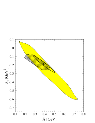
FIG. 2.: Impact of $1/m_{b}^{3}$ corrections on the extraction of $\bar{\Lambda},\lambda_{1}$. Shaded region: Higher order matrix elements estimated by dimensional analysis. Cross-hatched region: $\rho_{1}=0.13{\rm GeV}^{3},\,\rho_{2}=0$. Cross and ellipse show the values of $\bar{\Lambda},\lambda_{1}$ extracted without $1/m_{b}^{3}$ corrections but including the experimental statistical error.

Dimensional analysis suggests that the higher order matrix elements are all of order $\Lambda_{QCD}^{3}$, which can be used to make a quantitative estimate of the uncertainties in the extraction of $\bar{\Lambda},\lambda_{1}$. We vary the magnitude of $\rho_{1},{\cal T}_{1}-{\cal T}_{4}$ in eqs. (63) independently in the range $0-(0.5{\rm GeV})^{3}$, taking $\rho_{1}$ to be positive, as indicated by the vacuum saturation approximation, but making no assumption about the sign of the other matrix elements. Using the central values for $R_{1,2}^{exp}$ we find that $\bar{\Lambda},\lambda_{1}$ can lie inside the shaded region in Fig. 2. For comparison we also display the values of $\bar{\Lambda},\lambda_{1}$ extracted in Ref. [8] together with the ellipse showing the size of the statistical error of the experimental data. Clearly the theoretical uncertainties dominate the accuracy to which $\bar{\Lambda},\lambda_{1}$ can be extracted.

The situation can be improved only if we have some independent information on some or all of the higher dimension matrix elements. This requires either more experimental input or theoretical estimates of these matrix elements. $\rho_{1}$ can be estimated in the vacuum saturation approximation[15, 16, 11, 12, 17, 8], $\rho_{1}=(2\pi\alpha_{s}/9)m_{B}f_{B}^{2}$. The numerical value obtained this way is rather uncertain. Taking $\alpha_{s}=0.5$ and $f_{B}=270$MeV for purposes of illustration, we find $\rho_{1}\simeq 0.13{\rm GeV}^{3}$. No similar estimates exist for the other dimension-six matrix elements. $\rho_{2}$ vanishes in any non relativistic potential model, which may be taken as an indication that it is small relative to the other matrix elements. No estimates that go beyond dimensional analysis are available for the time ordered products.

The cross hatched region in Fig. 2 shows the range of $\bar{\Lambda},\lambda_{1}$ one obtains from setting $\rho_{1}=0.13{\rm GeV}^{3}$ and $\rho_{2}=0$ and varying the magnitude of the other matrix elements in the range $0-(0.5{\rm GeV})^{3}$. The previously extracted values of $\bar{\Lambda},\lambda_{1}$ are not excluded by this choice of $\rho_{1,2}$.

This method of extracting $\bar{\Lambda},\lambda_{1}$ is especially sensitive to higher order corrections since the constraints obtained form $R_{1}$ and $R_{2}$ give almost parallel bands in the $\bar{\Lambda}-\lambda_{1}$ plane. Thus small uncertainties in the theoretical expressions for $R_{1,2}$ result in large uncertainties in the extracted values of $\bar{\Lambda},\lambda_{1}$. The same applies to the very similar analysis in Ref. [18]. The rare decay $B\to X_{s}\gamma$ provides a way to extract a vertical band in the $\bar{\Lambda}-\lambda_{1}$ plane, but at present the experimental data does not allow a quantitative analysis[19]. Furthermore, as discussed in the introduction, it is not clear when HQET matrix elements extracted from different observables can be compared meaningfully[7, 9].

The second method for extracting information on $\bar{\Lambda},\lambda_{1}$ [9] was used to exclude some regions in the $\bar{\Lambda}-\lambda_{1}$ plane. The first and second moments of the invariant mass spectrum of the hadrons in the final state of the inclusive decay $B\to X_{c}\ell\nu$ turn out to give independent constraints on $\bar{\Lambda},\lambda_{1}$. Their definition involves the total decay rate at order $1/\overline{m}_{B}^{3}$. It can be obtained by combining the total rate at order $1/m_{b}^{2}$ from Ref. [3] with the contributions from local dimension-six operators eq. (38) and using eqs. (46). Finally eqs. (48) and (49) are used to eliminate the quark masses. Using the measured values for the meson masses and neglecting perturbative corrections we find to third order in $1/\overline{m}_{B}$:

$$\Gamma = \frac{|V_{cb}|^{2}G_{F}^{2}\overline{m}_{B}^{5}}{192\pi^{3}}\Bigg{[}0.3689-0.6080\frac{\bar{\Lambda}}{\overline{m}_{B}}-0.349\frac{\bar{\Lambda}^{2}}{\overline{m}_{B}^{2}}-1.175\frac{\lambda_{1}}{\overline{m}_{B}^{2}}-2.757\frac{\lambda_{2}}{\overline{m}_{B}^{2}}-0.11\frac{\bar{\Lambda}^{3}}{\overline{m}_{B}^{3}}$$ (64)

$$- 1.21\frac{\bar{\Lambda}\lambda_{1}}{\overline{m}_{B}^{3}}+2.95\frac{\bar{\Lambda}\lambda_{2}}{\overline{m}_{B}^{3}}-2.27\frac{\rho_{1}}{\overline{m}_{B}^{3}}+2.76\frac{\rho_{2}}{\overline{m}_{B}^{3}}-2.73\frac{{\cal T}_{1}}{\overline{m}_{B}^{3}}+0.55\frac{{\cal T}_{2}}{\overline{m}_{B}^{3}}-3.84\frac{{\cal T}_{3}}{\overline{m}_{B}^{3}}-2.76\frac{{\cal T}_{4}}{\overline{m}_{B}^{3}}\Bigg{]}.$$ (65)

Since none of the coefficients of the higher order matrix elements turn out to be abnormally large, dimensional analysis indicates that the $1/\overline{m}_{B}^{3}$ corrections to the total rate should not exceed 2%.

The hadronic moments are defined as

$$\langle(s_{H}-\overline{m}_{D}^{2})^{n}\rangle=\frac{1}{\Gamma}\int{\rm d}s_{H}{\rm d}E_{H}(s_{H}-\overline{m}_{D}^{2})^{n}\frac{{\rm d}\Gamma}{{\rm d}s_{H}{\rm d}E_{H}},$$ (66)

where $s_{H}=m_{B}^{2}-2m_{B}v\cdot q+q^{2}$ and $E_{H}=m_{B}-v\cdot q$ are the hadronic analogs of $\hat{s}_{0},\hat{E}_{0}$ defined in Sect. II. Using the relation between quark and hadron masses one can relate $s_{H},E_{H}$ to $\hat{s}_{0},\hat{E}_{0}$ and thus compute the moments using the expressions given in Ref. [9] together with eq. (33) and the usual substitution eqs. (46). We find to order $1/\overline{m}_{B}^{3}$:

$$\langle s_{H}-\overline{m}_{D}^{2}\rangle = \overline{m}_{B}^{2}\bigg{[}0.051\frac{\alpha_{s}}{\pi}+0.23\frac{\bar{\Lambda}}{\overline{m}_{B}}\left(1+0.43\frac{\alpha_{s}}{\pi}\right)+0.26\frac{1}{\overline{m}_{B}^{3}}(\bar{\Lambda}^{2}+3.9\lambda_{1}-1.2\lambda_{2})$$ (69)

$$+0.33\frac{1}{\overline{m}_{B}^{3}}(\bar{\Lambda}^{3}+6.6\bar{\Lambda}\lambda_{1}-1.7\bar{\Lambda}\lambda_{2}+7.0\rho_{1}+3.5\rho_{2}$$

$$+5.0{\cal T}_{1}+2.5{\cal T}_{2}+4.6{\cal T}_{3}+1.3{\cal T}_{4})\bigg{]}$$

$$\langle(s_{H}-\overline{m}_{D}^{2})^{2}\rangle = \overline{m}_{B}^{4}\bigg{[}0.0053\frac{\alpha_{s}}{\pi}+0.038\frac{\bar{\Lambda}}{\overline{m}_{B}}\frac{\alpha_{s}}{\pi}+0.065\frac{1}{\overline{m}_{B}^{3}}(\bar{\Lambda}^{2}-2.1\lambda_{1})$$ (71)

$$+0.14\frac{1}{\overline{m}_{B}^{3}}(\bar{\Lambda}^{3}+2.2\bar{\Lambda}\lambda_{1}+2.2\bar{\Lambda}\lambda_{2}-6.0\rho_{1}+1.7\rho_{2}-1.0{\cal T}_{1}-2.9{\cal T}_{2})\bigg{]}$$

where perturbative $\alpha_{s}$ corrections have been included. Rather that repeating the analysis presented in Ref. [9], we use these expressions to predict the values of the hadronic moments using the HQET matrix elements extracted from the lepton energy spectrum. The main reason for doing this is that the experimental measurement of the necessary branching fractions is not very precise. In particular ALEPH and CLEO quote only an upper bound for $Br(B\to D^{\ast}_{2}\ell\bar{\nu})$ [20, 21]. We extract an upper bound on this branching fraction from the theoretical prediction of the hadronic moments. A lower bound for the first hadronic moment is given by [9]

$$\langle s_{H}-\overline{m}_{D}^{2}\rangle \geq a\Bigg{[}(2.450{\rm GeV})^{2}-(1.975{\rm GeV})^{2}\Bigg{]}+b\Bigg{[}(2.010{\rm GeV})^{2}-(1.975{\rm GeV})^{2}\Bigg{]}$$ (73)

$$+c\Bigg{[}(1.869{\rm GeV})^{2}-(1.975{\rm GeV})^{2}\Bigg{]}$$

where $a,b$, and $c$ are the semileptonic branching fractions to $D^{\ast\ast},D^{\ast}$, and $D$ relative to the total semileptonic branching fraction. Using the measured ratio 0.41:0.59 for the decays to $D$ and $D^{\ast}$, we can write $b,c$ as functions of the branching fraction $a$ for $D^{\ast\ast}$:

$$b=0.59(1-a),\qquad c=0.41(1-a)$$ (74)

We take $a+b+c=1$, which is appropriate because we need only a lower bound on the hadronic moment. It is also implicitly assumed that the nonresonant semileptonic branching fraction below the $D^{\ast\ast}$ mass is negligible. Similarly, for the second hadronic moment we take

$$\langle(s_{H}-\overline{m}_{D}^{2})^{2}\rangle\geq a\Bigg{[}(2.450{\rm GeV})^{2}-(1.975{\rm GeV})^{2}\Bigg{]}^{2},$$ (75)

where small contributions from the ground state mesons $D,D^{\ast}$ have been neglected. We obtain theoretical predictions for the hadronic moments by substituting values of $\rho_{1},{\cal T}_{1}-{\cal T}_{4}$ and the corresponding values of $\bar{\Lambda},\lambda_{1}$ extracted from the lepton spectrum into eqs. (69). As before, we allow the magnitudes of $\rho_{1}$ and ${\cal T}_{1}-{\cal T}_{4}$ to vary in the range $0-(0.5{\rm GeV})^{3}$ with $\rho_{1}$ being positive. Imposing the constraint that the largest values of the hadronic moments obtained from this procedure be larger than the lower bounds eqs. (73),(75) we find the upper bound on the $D^{\ast\ast}$ branching fraction

$$a\leq 0.23\,.$$ (76)

This value is compatible with the experimentally measured values from ALEPH [20] ($Br(B\to D_{1}\ell\nu)=0.069\pm 0.015,Br(B\to D^{\ast}_{2}\ell\nu)<0.11$) and from CLEO[21]($Br(B\to D_{1}\ell\nu)=0.046\pm 0.013,Br(B\to D^{\ast}_{2}\ell\nu)<0.11$). It is also marginally consistent with the OPAL result $a=0.34\pm 0.07$[22]. Unless the matrix elements of dimension-six operators are even bigger than we have assumed, this implies that the branching fraction $a=0.27$ used in [9] is inconsistent with the values of $\bar{\Lambda},\lambda_{1}$ extracted from the lepton spectrum.

V Conclusions

We have calculated the $1/m_{b}^{3}$ contributions to various observables in the semileptonic decay $B\to X_{c}\ell\nu$. They are parametrized by the expectation values of two local and four nonlocal dimension-six operators. While the total rate is rather insensitive to the higher order corrections (1-2%), the values of $\bar{\Lambda},\lambda_{1}$ extracted from the lepton spectrum can be affected substantially. The theoretical uncertainties in the values of $\bar{\Lambda},\lambda_{1}$ are far larger than the statistical errors of the experimental measurements if the values of the higher order matrix elements are estimated using dimensional analysis. While one linear combination of $\bar{\Lambda}$ and $\lambda_{1}$ is still reasonably well constrained, it is not possible to extract individual values for $\bar{\Lambda}$ and $\lambda_{1}$ from the lepton spectrum only. The situation can be improved only if additional information on the size of the dimension-six matrix elements is used. Unfortunately no theoretical estimates are available for any of these matrix elements except $\rho_{1}$. The latter can be estimated in the vacuum saturation approximation, albeit with large uncertainties. Alternatively one can use additional experimental input, e.g., from $B\to X_{s}\gamma$ decays, to further constrain $\bar{\Lambda}$ and $\lambda_{1}$[19].

The values of $\bar{\Lambda},\lambda_{1}$ extracted from the lepton spectrum can be used to make theoretical predictions for the moments of the hadronic invariant mass spectrum. This amounts to expressing one observable in terms of other observables, a procedure that makes sense only if the perturbative series for this expression is reasonably well behaved. In order to determine whether this is the case it is necessary to know at least the next-to-leading order $\alpha_{s}$ corrections to all observables involved. Since they have not been computed for the lepton spectrum, there is at present no way we can check if predictions for the hadronic moments in terms of the HQET matrix elements extracted from the lepton spectrum satisfy this criterion.

Setting these considerations aside, we can predict the values of the hadronic moments in terms of $\bar{\Lambda},\lambda_{1}$ extracted from the lepton spectrum. The lower bounds for these moments depend on the branching fraction to $D^{\ast\ast}$, which is not well known experimentally. By demanding that not the whole range of predicted values of the hadronic moments be excluded by the lower bounds, we find an upper bound of 23% on the branching fraction to $D^{\ast\ast}$, if the higher order matrix elements are estimated by dimensional analysis. This value is consistent with the ALEPH and CLEO measurements.

A The Mass Formula

For comparison with experiments it is necessary to express the pole quark masses $m_{c}$ and $m_{b}$ in terms of HQET matrix elements and physical observables, e.g., the spin averaged meson masses $\overline{m}_{B}$ and $\overline{m}_{D}$, where $\overline{m}_{Meson}=(m_{P}+3m_{V})/4$. For this purpose one needs to know how quark masses are related to hadron masses at order $1/m_{b}^{3}$. Our starting point is the identity

$$m_{H}=\frac{V}{2}\frac{\langle H_{\infty}(v)\,|{\cal H}|\,H(v)\rangle}{\langle H_{\infty}(v)\,|\,H(v)\rangle}+h.c.\,,$$ (A1)

where $V$ is the normalization volume and ${\cal H}$ is the full Hamiltonian density including light degrees of freedom. This equation holds in the rest frame of the hadron. Then we split $\cal H$ into the leading term and the terms suppressed by powers of $1/m_{b}$, ${\cal H}={\cal H}_{0}+{\cal H}_{1}$, and use the fact that $|\,H_{\infty}(v)\rangle$ is an eigenstate of $\int d^{3}x{\cal H}_{0}$ with eigenvalue $m_{b}+\bar{\Lambda}$. The use of the Foldy-Wouthuysen-transformed fields eq. (13) ensures that there is no implicit dependence on $m_{b}$ in $h_{v}$. Also, there are no time-derivatives in the HQET Lagrangian beyond leading order, as can be seen e.g. from eq. (82) of Ref. [10]. Therefore we have ${\cal H}_{1}=-{\cal L}_{1}$. Using the Gell-Mann and Low theorem, the general expression for the hadron mass reads

$$m_{H}=m_{b}+\bar{\Lambda}-\frac{V}{2}\Bigg{[}\frac{\langle H_{\infty}(v)\,|{\cal L}_{1}\,T\exp\left(i\int d^{3}x\int^{0}_{-\infty}dt{\cal L}_{1}(x)\right)|\,H_{\infty}(v)\rangle}{\langle H_{\infty}(v)\,|T\exp\left(i\int d^{3}x\int^{0}_{-\infty}dt{\cal L}_{1}(x)\right)|\,H_{\infty}(v)\rangle}+h.c.\Bigg{]}.$$ (A2)

Expanding eq. (A2) to order $1/m_{b}^{3}$ we obtain the mass formula:

$$m_{H} = m_{b}+\bar{\Lambda}-\langle H_{\infty}(v)\,|{\cal L}_{I}+{\cal L}_{II}|\,H_{\infty}(v)\rangle$$ (A4)

$$-\left[\,{1\over 2}\langle H_{\infty}(v)\,|{\cal L}_{I}i\int d^{3}x\int_{-\infty}^{0}dt{\cal L}_{I}(x)|\,H_{\infty}(v)\rangle+h.c.\,\right],$$

where [10]

$${\cal L}_{II}=-{1\over{4m_{b}^{2}}}\bar{h}_{v}\,iD\!\!\!\!/_{\perp}(iv\cdot D)iD\!\!\!\!/_{\perp}\,h_{v}+{1\over{8m_{b}^{2}}}\bar{h}_{v}\,(iD\!\!\!\!/_{\perp})^{2}(iv\cdot D)\,h_{v}+{1\over{8m_{b}^{2}}}\bar{h}_{v}\,(iv\cdot D)(iD\!\!\!\!/_{\perp})^{2}\,h_{v},$$ (A5)

and ${\cal L}_{I}$ is given in eq. (43). Eq. (A4) contains expectation values of both local and nonlocal operators. The local part can be evaluated in terms of the matrix elements $\lambda_{1},\lambda_{2},\rho_{1}$ and $\rho_{2}$, while the nonlocal matrix elements can be expressed through ${\cal T}_{1}-{\cal T}_{4}$ defined in eqs. (44). In terms of these matrix elements the meson mass is given by

$$m_{H}=m_{b}+\bar{\Lambda}-\frac{\lambda_{1}+d_{H}\lambda_{2}}{2m_{b}}+\frac{\rho_{1}+d_{H}\rho_{2}}{4m_{b}^{2}}-\frac{{\cal T}_{1}+{\cal T}_{3}+d_{H}({\cal T}_{2}+{\cal T}_{4})}{4m_{b}^{2}},$$ (A6)

in agreement with Refs. [10, 11].