I will discuss the current status of the determination of $\alpha(m_{Z})$ and $\alpha_{s}(m_{Z})$, emphasizing the pitfalls that one must avoid in performing statistical analyses.

Talk presented at the Yukawa International Seminar (YKIS) ’95
“From the Standard Model to Grand Unified Theories”
Kyoto, Japan, August 21–25, 1995.

CERN–TH/96–79

March 1996

The Status of the Determination of $\alpha(m_{Z})$ and $\alpha_{s}(m_{Z})$.

1 Introduction

Precise determinations of the values of $\alpha(m_{Z})$ and $\alpha_{s}(m_{Z})$ are important in the context of both the Standard Model (SM) and Grand Unified Theories (GUT’s) which are the two major themes of this conference.

In the SM, the values of $\alpha(m_{Z})$ and $\alpha_{s}(m_{Z})$ are necessary as inputs in calculating the predictions for observables at the $Z$–mass scale. The accuracy in which they are known is reflected directly onto the accuracy of the SM predictions that must be compared with the precision electroweak measurements at LEP/SLC. Therefore, if one wishes to test the SM at the level of radiative corrections and/or detect virtual effects of new physics in the LEP/SLC measurements, one needs to know $\alpha(m_{Z})$ and $\alpha_{s}(m_{Z})$ to very high accuracy. This point is well summarized in the talk by Hagiwara in this proceedings [1].

In the case of GUT’s, the three gauge couplings of $SU_{C}(3)\times SU_{L}(2)\times U_{Y}(1)$ must coincide when evolved up to the GUT scale using renormalization group equations (RGE’s). Whether they actually coincide or not depends on their initial values at $s=m_{Z}^{2}$, and the particle spectrum contributing to the RGE’s. Therefore, precise values of $\alpha(m_{Z})$ and $\alpha_{s}(m_{Z})$ will provide important constraints on the particle content and their masses for any given GUT [2].

In this talk, I will discuss the current status of the determination of $\alpha(m_{Z})$ and $\alpha_{s}(m_{Z})$. To avoid this talk from being a simple update of Ref. ?, I have shifted my emphasis somewhat to the problems in statistical analyses that one encounters when trying to extract these numbers from experimental data.

For $\alpha(m_{Z})$, I will give a comprehensive review of all the recent attempts to determine its value from the $\sigma(e^{+}e^{-}\rightarrow hadrons)$ data [4, 5, 6, 7, 8, 9, 10] and clarify where these analyses differ from each other. In particular, I will emphasize the problems that must be addressed in the treatment of the experimental data, and whether any of these analyses have succeeded in doing so or not. My conclusion here will be somewhat different from the one I gave at the conference, partly due to the fact that the details of the Swartz 1995 analysis has been made available[10] and it can now be given a proper evaluation, and partly due to my better understanding of the problem.

For $\alpha_{s}(m_{Z})$, I will not be reviewing all the different methods of determining $\alpha_{s}(m_{Z})$ and how reliable they are, since thorough and excellent reviews on the subject by experts in the field already exist in the literature [11, 12]. I will instead focus on the problem of determining $\alpha_{s}(m_{Z})$ from the $Z$–lineshape parameter $R_{\ell}=\mathchar 28928\relax(Z\rightarrow hadrons)/\mathchar 28928\relax(Z\rightarrow\ell^{+}\ell^{-})$ at LEP and discuss an interesting (but erroneous) speculation of Ref. ? which claims that the error on $R_{\ell}$, and thus $\alpha_{s}(m_{Z})$ determined from it, may be grossly underestimated based on an exotic (to particle physicists) statistical analysis.

2 The value of $\alpha(m_{Z})$

Fig.  1: Evaluations of $\alpha(m_{Z})$ by different authors. All values have been rescaled to $m_{Z}=91.1887$ GeV and the top quark contribution has been removed.

The best determination of $\alpha(m_{Z})$ until late 1994 had been that of Jegerlehner[5] from 1991 which was

$$\alpha^{-1}(m_{Z})=128.87\pm 0.12.$$ (2.1)

As an example of how this uncertainly in $\alpha(m_{Z})$ affects SM predictions, I quote the calculation of $\sin^{2}\theta_{\rm eff}^{\rm lept}$ based on this value using the FORTRAN program ZFITTER 4.9[15] which gives

$$\sin^{2}\theta_{\rm eff}^{\rm lept}=0.2319\pm 0.0003$$ (2.2)

for the SM with $m_{t}=180$GeV and $m_{H}=300$GeV. The 0.1% error on $\alpha(m_{Z})$ has propagated directly into a similar error on $\sin^{2}\theta_{\rm eff}^{\rm lept}$. On the other hand, the experimental error on $\sin^{2}\theta_{\rm eff}^{\rm lept}$ has been decreasing steadily. Currently, the averaged value of $\sin^{2}\theta_{\rm eff}^{\rm lept}$ from all asymmetry measurements at LEP and SLC is at[14]

$$\sin^{2}\theta_{\rm eff}^{\rm lept}=0.23143\pm 0.00028.$$ (2.3)

Clearly, an improvement on the knowledge of $\alpha(m_{Z})$ is called for given that the experimental error is now smaller than the theoretical error, and can be expected to decrease even further.

During the past year or so, several authors have independently made attempts to reevaluate the value of $\alpha(m_{Z})$ through careful reanalyses of existing $\sigma(e^{+}e^{-}\rightarrow hadrons)$ data [6, 7, 8, 9, 10]. The hope was that the uncertainty in $\alpha(m_{Z})$ could be reduced since some new data on $\sigma(e^{+}e^{-}\rightarrow hadrons)$ had been released[16, 17, 18], and the $O(\alpha_{s}^{3})$ QCD correction to the cross section[19] together with a better determination of $\alpha_{s}(m_{Z})$[11, 12] was now available. The resulting new values of $\alpha(m_{Z})$ are shown in Fig. 1 together with a couple of older values.

Comparing the five new evaluations, we see that the four most recent ones are all more or less consistent with each other and the Jegerlehner ’91 value with no significant decrease in the error. The only number which is slightly off is the Swartz ’94 value from Ref. ? which was updated by Swartz himself in Ref. ?.

Due to this agreement between different evaluations, it does not really matter which of these four numbers is used as the standard value of $\alpha(m_{Z})$ from a practical point of view. However, since we must decide on one number anyway, we may as well choose the one which can be considered to give the best estimate of the true value of $\alpha(m_{Z})$.

In the following, I will review how the analyses shown in Fig. 1 differ from each other so that we may make an informed decision. But before I begin, I will first review the definition of $\alpha(m_{Z})$ and how it can be determined from the $\sigma(e^{+}e^{-}\rightarrow hadrons)$ data so that we can have a clear understanding of the issues that must be addressed.

2.1. The Definition of $\alpha(m_{Z})$

The quantity whose value is usually quoted as that of the “effective QED coupling constant at the $Z$ mass scale” is defined as

$$\alpha^{-1}(m_{Z})=\alpha^{-1}\left[1-\mathchar 28929\relax\alpha(m_{Z})\right]$$ (2.4)

with

$$\mathchar 28929\relax\alpha(s)=4\pi\alpha{\rm Re}\left[\mathchar 28933\relax^{\prime}_{QQ}(s)-\mathchar 28933\relax^{\prime}_{QQ}(0)\right].$$ (2.5)

Here, $\mathchar 28933\relax^{\prime}_{QQ}(s)$ is the photon vacuum polarization function defined as

$$\int d^{4}x\,e^{iq\cdot x}\langle J_{Q}^{\mu}(x)J_{Q}^{\nu}(0)\rangle=i(q^{2}g^{\mu\nu}-q^{\mu}q^{\nu})\mathchar 28933\relax^{\prime}_{QQ}(s)$$ (2.6)

where $J_{Q}^{\mu}(x)$ is the electromagnetic current modulo the coupling constant $e$.

It has been customary to include only the light fermion contributions to $\mathchar 28929\relax\alpha(m_{Z})$. The top contribution had been excluded from $\mathchar 28929\relax\alpha(m_{Z})$ because the top mass was unknown until quite recently[20] (though care is needed when comparing results since recent authors include it) and the $W$ contribution was also excluded to keep the definition of $\alpha(m_{Z})$ gauge independent. They are also numerically small compared to the light fermion contribution since the $W^{+}W^{-}$ and $t\bar{t}$ thresholds are above the $Z$ mass so that they do not contribute logarithms to the running of $\alpha(s)$ between $s=0$ and $s=m_{Z}^{2}$. I will adhere to this convention in this talk and only discuss the contribution of light fermions. Readers who are interested in how the value of $\alpha(m_{Z})$ will change when the $t\bar{t}$ and the $W^{+}W^{-}$ pinch contributions are included are referred to Table I of the talk by Hagiwara[1].

2.2. Contribution of the light fermions

The contribution of the leptons to $\mathchar 28929\relax\alpha$ can be calculated accurately in perturbation theory and one finds

$$\mathchar 28929\relax\alpha_{leptons}(m_{Z}^{2}) = \sum_{\ell=e,\mu,\tau}\frac{\alpha}{3\pi}\left[-\frac{8}{3}+\beta_{\ell}^{2}-\frac{1}{2}\beta_{\ell}(3-\beta_{\ell}^{2})\ln\left(\frac{1-\beta_{\ell}}{1+\beta_{\ell}}\right)\right]$$ (2.7)

$$= \sum_{\ell=e,\mu,\tau}\frac{\alpha}{3\pi}\left[\ln\left(\frac{m_{Z}^{2}}{m_{\ell}^{2}}\right)-\frac{5}{3}+O\left(\frac{m_{\ell}^{2}}{m_{Z}^{2}}\right)\right]$$ (2.8)

$$= 0.03142,$$ (2.9)

where $\beta_{\ell}=\sqrt{1-4m_{\ell}^{2}/m_{Z}^{2}}$.

On the other hand, the contribution of the five light quarks ($u,d,s,c,b)$ to $\mathchar 28929\relax\alpha$ cannot be calculated perturbatively. Instead, unitarity and the analyticity of $\mathchar 28933\relax^{\prime}_{QQ}(s)$ is used to write

$$\mathchar 28929\relax\alpha^{(5)}_{hadrons}(s)=\frac{\alpha s}{3\pi}{\rm P}\int_{4m_{\pi}^{2}}^{\infty}ds^{\prime}\frac{R(s^{\prime})}{s^{\prime}(s-s^{\prime})},$$ (2.10)

where

$$R(s)\equiv\frac{3s}{4\pi\alpha^{2}(s)}\sigma(e^{+}e^{-}\rightarrow\gamma^{*}\rightarrow hadrons)=-12\pi{\rm Im}\mathchar 28933\relax^{\prime}_{QQ}(s)$$ (2.11)

and the functional form of $R(s)$ is extracted from experiment. It is this reliance on the experimental values of $R(s)$, which are currently accompanied by large experimental errors, that we end up with a relatively large error on $\alpha(m_{Z})$ even though the fine structure constant $\alpha$ is known to extreme accuracy.

2.3. Problems with using $R(s)$

There are a couple of problems that must be addressed when using the experimental values of $R(s)$ to calculate $\alpha(m_{Z})$.

First, the data for $R(s)$ are only available for discrete, scattered values of $s$. One must therefore interpolate between, and extrapolate beyond the available data points to make use of Eq. 2.10.

Two methods have been used in the literature to deal with this problem. The first is to connect the data points directly with straight lines and perform trapezoidal integration[4, 5, 8], and the second is to guess the functional form of $R(s)$ and fit it to the data[4, 6, 7, 10].

Both methods have their pros and cons. Trapezoidal integration is free from human prejudice about the functional form of $R(s)$ but it is difficult to take into account the experimental errors properly: sparsely distributed precise data points may not get the appropriate weight relative to the densely spaced data points with larger errors, and possible correlations between errors are not accounted for. Connecting two data points that are far apart with a straight line will also introduce errors in regions where $R(s)$ is changing rapidly. (A kind of ‘human prejudice’ in a sense.)

On the other hand, fitting a guessed functional form to the data has the advantage that experimental errors are easier to take into account (though care is needed in treating normalization errors[21] as will be discussed later). However, the result will depend on the choice of the fit function and its parameterization, and systematic errors and biases will be introduced that are difficult to estimate.

The two methods are often combined (e.g. fitting the Gounaris–Sakurai[22] form to the $\rho$[23], Breit–Wigner forms to the narrow resonances, and using trapezoidal integration for the continuum) and are supplemented by the use of perturbative QCD for the high energy tail of $R(s)$.

Secondly, the experimental values of $R(s)$ are always accompanied by experimental errors, both statistical and systematic, and often rather large.

The systematic error consists of uncertainties in the measurement/monitoring of collider luminosity ${\cal L}$, Monte Carlo calculation of the detection efficiency $\varepsilon$, and radiative corrections $\delta$ that are introduced when converting the measured event rate $N$ into the cross section $\sigma$ through the relation

$$N=\sigma{\cal L}\varepsilon(1+\delta).$$ (2.12)

It is therefore a normalization uncertainty.

Obviously, such normalization errors on data points belonging to the same experiment are 100% correlated. This type of correlation of systematic errors within a single experiment is called a Type I correlation in Ref. ?.

However, there can also be strong correlations between the normalization errors on data points belonging to two different experiments if they use the same collider, same knowledge of radiative corrections, event generators based on similar models, same background estimation methods, same detector response models, etc. This type of correlation of systematic errors between different experiments is called a Type II correlation in Ref. ?. Their exact size is difficult to estimate, but they nevertheless exist.

Taking such correlations into account when extracting $R(s)$ from data has important consequences as we will see later.

2.4. Recent estimates of $\alpha(m_{Z})$

Let us now start our tour of all the different analyses shown in Fig. 1 and see how they address the problems discussed above. The order in which they will be presented is not necessarily chronological, but what I deem appropriate to contrast the differences.

2.4.1. The analysis of Burkhardt et al.

At the time when LEP started running in 1989, the most accurate determination of $\mathchar 28929\relax\alpha^{(5)}_{hadrons}(m_{Z}^{2})$ was that given by Burkhardt et al. in Ref. ?:

$$\mathchar 28929\relax\alpha^{(5)}_{hadrons}(m_{Z}^{2})=0.0286\pm 0.0009.$$ (2.13)

(Actually, Ref. ? reports the value of $\mathchar 28929\relax\alpha^{(5)}_{hadrons}(s)$ at $\sqrt{s}=92$ GeV. Rescaling to $\sqrt{s}=m_{Z}=91.1887$ GeV gives the above value[24].) This value was calculated using the following three methods of interpolation

1. Trapezoidal integration for the continuum and the $\rho$.
   Breit–Wigner forms for the narrow resonances.

2. Trapezoidal integration for the continuum after a partial smoothing out of the $R(s)$ data. (Ref. ? does not give any detail on how the smoothing was done.)
   Breit–Wigner forms for the narrow resonances.

3. Breit–Wigner forms for the $\rho$ and narrow resonances.
   Linear interpolation in $W=\sqrt{s}$ for every few points in the continuum.

In all three cases, perturbative QCD (at $O(\alpha_{s}^{2})$) was used for $R(s)$ above $40$ GeV. The difference in $\mathchar 28929\relax\alpha^{(5)}_{hadrons}(m_{Z}^{2})$ due to the difference in the method of interpolation was found to be negligible compared to the statistical error.

Eq. 2.13 corresponds to

$$\alpha^{-1}(m_{Z}) = \alpha^{-1}\left[1-\mathchar 28929\relax\alpha_{leptons}(m_{Z}^{2})-\mathchar 28929\relax\alpha^{(5)}_{hadrons}(m_{Z}^{2})\right]$$ (2.14)

$$= 128.81\pm 0.12$$ (2.15)

and results in an error of about 0.1% in $\alpha(m_{Z})$. The region below the bottom threshold contributed about $1/3$ of $\mathchar 28929\relax\alpha^{(5)}_{hadrons}(s)$, and 80% of the error.

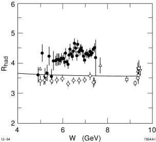
Fig.  2: Comparison of MARK I (black circles) and Crystal Ball (while diamonds) data. Only statistical errors are shown. The solid line shows the perturbative QCD result.

2.4.2. The analysis of Jegerlehner

The result of Ref. ? was subsequently updated in 1991 by Jegerlehner[5], who was one of the original authors, in which the data from the MARK I collaboration[27] in the energy region 5–7.4 GeV were replaced by the more accurate data from the Crystal Ball collaboration[28]. Fig. 2 shows the data of both collaborations in the energy range in question, together with the perturbative QCD result. The method of integration was the same as method No. 1 of Ref. ? and the result was

$$\mathchar 28929\relax\alpha^{(5)}_{hadrons}(m_{Z}^{2})=0.0282\pm 0.0009,$$ (2.16)

with no change in the size of the error. This corresponds to

$$\alpha^{-1}(m_{Z})=128.87\pm 0.12$$ (2.17)

which had been the standard value until late 1994.

2.4.3. The analysis of Eidelman and Jegerlehner

The 1991 Jegerlehner value was again updated by Eidelman and Jegerlehner in Ref. ? to include new data[16, 17, 18] in the analysis. Again trapezoidal integration was used.

This reference goes into some detail on how experimental errors were taken into account. In order to prevent sparsely distributed precise data points from getting less weight than densely spaced data points with large errors, which is one of the problems inherent in trapezoidal integration, Eidelman and Jegerlehner used the following two methods:

• When more than one experiment gave results in the same energy region, the contribution to $\mathchar 28929\relax\alpha^{(5)}_{hadrons}(m_{Z}^{2})$ from that energy region was calculated using trapezoidal integration for each experiment separately, and then the resulting integrals were combined by taking a error weighted average.

• Data from different experiments in the same energy region were combined by taking local error weighted averages, and trapezoidal integration was performed on the combined data.

Both methods were found to give similar results which is not too surprising since the local average for a point $s$ was defined as the average of the $R(s)$ values obtained by linear interpolation between the nearest data points.

After subtracting out the top quark contribution from the value reported in Ref. ?, we obtain

$$\mathchar 28929\relax\alpha^{(5)}_{hadrons}(m_{Z}^{2})=0.02804\pm 0.00065,$$ (2.18)

and

$$\alpha^{-1}(m_{Z})=128.89\pm 0.09,$$ (2.19)

which agrees very well with the previous estimate[5].

2.4.4. The analysis of Burkhardt and Pietrzyk

The recent analysis of Burkhardt and Pietrzyk in Ref. ? is another update of Ref. ?, but this time using method No. 3, i.e. linear interpolation in $W=\sqrt{s}$ for every few points in the continuum.

In the $5-7.4$ GeV energy range, an error weighted average of the MARK I[27] and Crystal Ball[28] data was used instead of discarding the MARK I data altogether as in Refs. ?, ?, ?, ?. New data from Refs. ?, ?, ? were also included. The resulting value of $\mathchar 28929\relax\alpha^{(5)}_{hadrons}(m_{Z}^{2})$ was

$$\mathchar 28929\relax\alpha^{(5)}_{hadrons}(m_{Z}^{2})=0.0280\pm 0.0007,$$ (2.20)

which corresponds to

$$\alpha^{-1}(m_{Z})=128.89\pm 0.09.$$ (2.21)

2.4.5. The analysis of Martin and Zeppenfeld

The analysis of Martin and Zeppenfeld in Ref. ? distinguishes itself from all the other analyses in its extensive use of perturbative QCD. In table I, I list the energy ranges in which different authors have applied perturbative QCD. (Though I also list the values of $\alpha_{s}(m_{Z})$ that were used, at the current level of accuracy, the difference is insignificant. Changing the value of $\alpha_{s}(m_{Z})$ has little effect on the resulting value of $\alpha(m_{Z})$.)

In the two energy regions 3–3.9 GeV and 6.5–$\infty$ GeV, Martin and Zeppenfeld express $R(s)$ as the perturbative QCD value plus the $J/\mathchar 28937\relax$, $\mathchar 28937\relax$, and $\mathchar 28935\relax$ resonances. The DASP[25], PLUTO[26], MARK I[27], and Crystal Ball[28] data are all rescaled to fit the perturbative QCD result in these energy ranges, and the rescaled data is used to resolve a couple of resonances in the energy region between 3.9 and 6.5 GeV. See Fig. 3.

This kind of collective rescaling of data is not as arbitrary as it may seem. The normalization errors reported by the experiments shown in Fig. 3 are 15% (DASP), 12% (PLUTO), 10$\sim$20% (MARK I), and 5.2% (Crystal Ball), respectively, so the rescaled data are well within $1\!\sim\!2\sigma$ of their original values. If one believes that perturbative QCD is valid in this energy range, then it is quite natural to use it to fix the data to the ‘correct’ normalization.

Table  I: Comparison of the reliance on perturbative QCD in the evaluation of $\alpha(m_{Z})$ between different authors.

Author	Energy Range (GeV)	Order in $\alpha_{s}$	$\alpha_{s}(m_{Z})$
Burkhardt et al.[4, 24] (1989)	$40-\infty$	$2$	$0.12\pm 0.02$
Jegerlehner[5] (1991)	$40-\infty$	$2$	$0.117\pm 0.010$
Swartz[6] (1994)	$15-\infty$	$3$	$0.125\pm 0.005$
Martin & Zeppenfeld[7] (1994)	$3-3.9$, $6.5-\infty$	$3$	$0.118\pm 0.007$
Eidelman & Jegerlehner[8] (1995)	$40-\infty$	$3$	$0.126\pm 0.005$
Burkhardt and Pietrzyk[9] (1995)	$12-\infty$	$3$	$0.124\pm 0.020$
Swartz[10] (1995)	$15-\infty$	$3$	$0.116\pm 0.005$

Due to the heavy reliance on perturbative QCD in this analysis, and consequently the relatively light reliance on experimental data, the uncertainty in $\mathchar 28929\relax\alpha^{(5)}_{hadrons}(m_{Z}^{2})$ is reduced. The value quoted in Ref. ? is

$$\mathchar 28929\relax\alpha^{(5)}_{hadrons}(m_{Z}^{2})=0.02739\pm 0.00042,$$ (2.22)

which corresponds to

$$\alpha^{-1}(m_{Z})=128.98\pm 0.06.$$ (2.23)

Fig.  3: The rescaling of data in Ref. ?. Only statistical errors are shown.

2.4.6. The analyses of Swartz

The analyses by Swartz in Refs. ? and ? fit a smooth function described by polynomials in $W=\sqrt{s}$ to the continuum part of $R(s)$. Resonances were described by Breit–Wigner forms as usual, and perturbative QCD (at $O(\alpha_{s}^{3})$) was used above 15 GeV.

The Swartz analyses distinguish themselves as the first attempts to treat Type I and Type II correlations on a firm statistical basis.

In his first analysis[6], Swartz used a standard technique in fitting his function $R_{fit}(s;a_{k})$ to the $R(s)$ data. Namely, the parameters $a_{k}$ which parameterized his function were chosen to minimize the $\chi^{2}$ defined as

$$\chi^{2}=\sum_{i,j}\left[R_{i}-R_{fit}(s_{i};a_{k})\right]V_{ij}^{-1}\left[R_{j}-R_{fit}(s_{j};a_{k})\right],$$ (2.24)

where $R_{i}$ is the experimental value of the $i$-th measurement at $s_{i}$, and $V^{-1}=(V_{ij}^{-1})$ is the inverse of the variance–covariance matrix $V=(V_{ij})$:

$$V_{ij}=\langle\mathchar 28929\relax R_{i}\,\mathchar 28929\relax R_{j}\rangle.$$ (2.25)

$\mathchar 28929\relax R_{i}=R(s_{i})-R_{i}$ is the difference between the true value of $R(s_{i})$ and the measured value $R_{i}$, and $\langle{\cal O}\rangle$ denotes the expectation value of ${\cal O}$.

Following Swartz, I denote the uncorrelated point to point error on $R_{i}$ as $\sigma_{i}(ptp)$ and the correlated normalization error as $\sigma_{i}(norm)$:

$$R(s_{i})=R_{i}\pm\sigma_{i}(ptp)\pm\sigma_{i}(norm).$$ (2.26)

Assuming that both Type I and Type II correlations are 100% when they are present, $V_{ij}$ is given by

$$V_{ij}=\left\{\begin{array}[]{ll}\sigma_{i}^{2}(ptp)+\sigma_{i}^{2}(norm)&i=j\\ \sigma_{i}(norm)\sigma_{j}(norm)&\mbox{$i\neq j$, with correlation }\\ 0&\mbox{$i\neq j$, no correlation}\end{array}\right.$$ (2.27)

Using this expression for $V_{ij}$, Swartz obtained the fit shown with a solid line in Fig. 5. For comparison, Fig. 5 also shows the fit when all correlations are neglected with a broken line.

The difference between the two cases is significant. When the uncorrelated fit was used, Swartz found that he reproduced the result of Ref. ?, in good agreement with Refs. ?, ?, and the observation of Ref. ? that the value of $\mathchar 28929\relax\alpha^{(5)}_{hadrons}(m_{Z}^{2})$ is relatively insensitive to the interpolation method. However, when he used the correlated fit, he found

$$\mathchar 28929\relax\alpha^{(5)}_{hadrons}(m_{Z}^{2})=0.02672\pm 0.00075,$$ (2.28)

and

$$\alpha^{-1}(m_{Z})=129.07\pm 0.10,$$ (2.29)

which differed from Eq. 2.17 by $0.20\approx 2\sigma$.

This analysis has been criticized[8] on the grounds that including normalization errors in the correlation matrix will produce a fit which is biased towards smaller values of $R(s)$. This effect is beautifully explained in a very nice paper by D’Agostini[21]. Since I feel that this is a very important point which everyone should know about, I have reproduced the basic argument in Appendix A.

Swartz has subsequently updated his analysis to correct for this problem and also to include some data[29] which was missing from his first analysis[10]. The new fit to the continuum part of $R(s)$ is shown in Fig. 5, and was obtained by minimizing

$$\chi^{2}=\sum_{i}\frac{[R_{i}-(1+\lambda_{j}\alpha_{i})R_{fit}(s_{i};a_{k})]^{2}}{\sigma_{i}^{2}(ptp)}+\sum_{j}\lambda_{j}^{2},$$ (2.30)

where $\alpha_{i}=\sigma_{i}(norm)/R_{i}$, and $\lambda_{j}$ are normalization parameters which account for collective rescaling of the data points in the $j$-th data set. (cf. Appendix A.) Using this new fit, Swartz obtained

$$\mathchar 28929\relax\alpha^{(5)}_{hadrons}(m_{Z}^{2})=0.02752\pm 0.00046,$$ (2.31)

and

$$\alpha^{-1}(m_{Z})=128.96\pm 0.06.$$ (2.32)

The interesting thing about this result is that only 1/3 of the difference between this value and the previous one given in Eq. 2.29 is accounted for by the change from a biased to an unbiased fit. The remaining 2/3 of the shift is due to the inclusion of a single data point at $W=3.670$ GeV from the Crystal Ball collaboration [29] which had a much smaller normalization error than all other data points in the vicinity. The effect of this point can be clearly seen by comparing Fig. 5 and the uncorrelated fit in Fig. 5. Due to normalization correlations, the entire fit function below $W=3.670$ GeV has been pulled upwards and statistical fluctuations around this function suppressed. This accounts for the larger value of $\mathchar 28929\relax\alpha^{(5)}_{hadrons}(m_{Z}^{2})$ and smaller error.

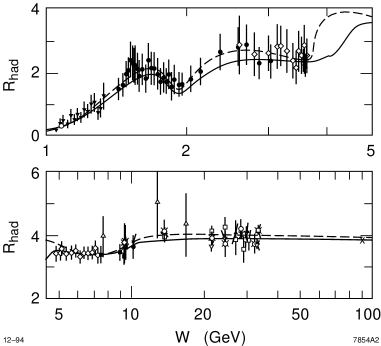
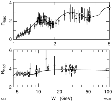
Fig.  4: Fit to the continuum part of $R(s)$ with (solid line) and without (broken line) correlations from normalization errors. The difference between the two in the 3.6–5 GeV region is due to a different treatment of the higher $\mathchar 28937\relax$ resonances. The error bars on the data points show the total (statistical+systematic) error.

Fig.  5: The new fit by Swartz. The Crystal Ball data point at $W=3.670$ GeV is hidden in the cluster of points in the vicinity. The error bars show the total error.

Fig.  6: Comparison of the new fit by Swartz (broken line) and the trapezoidal integration of Eidelman and Jegerlehner (solid line).

2.5. Discussion

In Refs. ?, ?, ?, ? the difficulty of dealing with Type II correlations is discussed, but no strategy is presented as to how they are actually dealt with. Type I correlations are not even mentioned. Given that the uncorrelated fit of Swartz[6] reproduced the result of Refs. ?, ?, ?, I believe it safe to assume that none of these analyses took Type I or Type II correlations into account. The independence of the result on the interpolation method found in these works can also be understood as due to the neglect of normalization correlations.

In the Swartz ’95 analysis[10], correlated data are collectively rescaled to obtain the best fit. Both Type I and Type II correlations are considered. The resulting fit function is quite different from the one integrated in the trapezoidal method of Ref. ? as shown in Fig. 6. In my opinion, this analysis makes the best use of all the information available in the experimental data. However, the Swartz estimate is also susceptible to change drastically by the inclusion of new data. This is exemplified by the effect of the one data point from Crystal Ball at $W=3.670$ GeV which ‘fixed’ the global normalization of $R(s)$ below this point. If this point had not been included, then the estimate would have been much closer to the Swartz ’94 value[6]. Every time a new and precise data point is included in the analysis, the correlations will cause a ripple effect which may shift the entire function upwards or downwards. Therefore, to be on the conservative side, the error should be doubled when using the Swartz estimate.

The Martin and Zeppenfeld value[7] is obtained by using perturbative QCD to rescale the experimental data, so if one believes in perturbative QCD down to 3 GeV, then this would be a good value to use. One must remember, however, that theoretical prejudice has entered into the $\alpha(m_{Z})$ value. The error is also artificially small due to use of perturbative QCD and cannot be justified by the data alone. To be on the conservative side, the error should be doubled in this case also.

My conclusion is that the Swartz ’95 analysis with doubled errors is probably the best estimate of $\alpha(m_{Z})$ currently available. Namely,

$$\alpha^{-1}(m_{Z})\approx 129.0\pm 0.1.$$ (2.33)

(Extra digits would be meaningless.) A better determination of $\alpha(m_{Z})$ is impossible with the current quality of $R(s)$ data. Any further improvement requires better measurements of $R(s)$ in the low energy region below 10 GeV[9].

3 The Value of $\alpha_{s}(m_{Z})$

3.1. Current status

In the case of $\alpha_{s}(m_{Z})$, there exist more than one way to determine it’s value. Refs. ?, ? give comprehensive overviews of the many ways to measure $\alpha_{s}(m_{Z})$. In table II, I list some of the most recent determinations of $\alpha_{s}(m_{Z})$ using various techniques.

Table  II: Current status of the determination of $\alpha_{s}(m_{Z})$.

Method of Measurement	$\alpha_{s}(m_{Z})$
Deep Inelastic Scattering[12]	$0.112\pm 0.005$
GLS sum rule[12]	$0.108\pm 0.008$
$\mathchar 28935\relax$ decay into 3 gluons[30]	$0.108\pm 0.005$
Voloshin[31]	$0.109\pm 0.001$
Lattice[32]	$0.112\pm 0.007$
LEP
$Z$ lineshape data[14]	$0.125\pm 0.004$
$R_{\ell}$ only[14]	$0.126\pm 0.005$
event shapes and jet rates[33]	$0.123\pm 0.006$
SLD
event shapes and jet rates[34]	$0.120\pm 0.008$

As pointed out by Shifman[12], all the low energy determinations of $\alpha_{s}(m_{Z})$ are clustered around $\alpha_{s}(m_{Z})=0.11$ while all the high energy determinations at LEP/SLC are clustered around $\alpha_{s}(m_{Z})=0.125$. This discrepancy, with a related discrepancy between the SM prediction and experiment in $R_{b}$, can be interpreted as a sign of new physics as discussed in the talk by Hagiwara[1].

Another interesting possibility that was pointed out by Consoli and Ferroni in Ref. ? was that the error on the LEP value of $R_{\ell}=\mathchar 28928\relax(Z\rightarrow hadrons)/\mathchar 28928\relax(Z\rightarrow\ell^{+}\ell^{-})$ may be grossly underestimated and that the actual error may be roughly five times larger. If that were the case, the error on the value of $\alpha_{s}(m_{Z})$ extracted from $R_{\ell}$ will be enhanced also by the same factor and the discrepancy between the low energy and high energy determinations may vanish.

Unfortunately (or fortunately, depending on your point of view) their argument is flawed. In the following, I will give an outline of the Consoli and Ferroni discussion and point out where their logic is problematic.

Table  III: $R_{\ell}$ values from LEP 1994 data.

	ALEPH	DELPHI	L3	OPAL
$R_{e}$	$20.67\pm 0.13$	$20.96\pm 0.16$	$20.94\pm 0.13$	$20.90\pm 0.13$
$R_{\mu}$	$20.91\pm 0.14$	$20.60\pm 0.12$	$20.93\pm 0.14$	$20.855\pm 0.097$
$R_{\tau}$	$20.69\pm 0.12$	$20.64\pm 0.16$	$20.70\pm 0.17$	$20.91\pm 0.13$

Fig.  7: The Distribution of LEP 1994 $R_{\ell}$ data. The arrow indicates the weighted average.

Fig.  8: The Distribution of LEP 1995 $R_{\ell}$ data. The arrow indicates the weighted average.

3.2. The Argument of Consoli and Ferroni

The argument of Consoli and Ferroni[13] was based on the $R_{\ell}$ values from the 1994 LEP data. In Table. III, I list the data for $R_{e}$, $R_{\mu}$, and $R_{\tau}$ from the four LEP experiments. Neglecting small correlations and using the standard error weighted average formula

$$\bar{x}=\frac{\sum_{i}\frac{x_{i}}{\sigma_{i}^{2}}}{\sum_{i}\frac{1}{\sigma_{i}^{2}}},\qquad\frac{1}{\bar{\sigma}^{2}}=\sum_{i}\frac{1}{\sigma_{i}^{2}},$$ (3.1)

the average of the 12 values listed in Table III gave

$$R_{\ell}=20.795\pm 0.040$$ (3.2)

which corresponded to

$$\alpha_{s}(m_{Z})=0.126\pm 0.006.$$ (3.3)

The observation of Consoli and Ferroni was that when the 12 data points were plotted in a histogram, it looked like Fig. 8 with two distinct peaks sandwiching the average value. This made them question whether the data points were normally distributed around a common peak and whether it was correct to use Eq. 3.1.

In order to answer this question, they calculated a quantity called the kurtosis defined by

$$\gamma=\mu_{4}/\mu_{2}^{2}-3,$$ (3.4)

where $\mu_{n}=\int(x-\bar{x})^{n}f(x)dx$ is the $n$-th moment of the distribution, and found it to be $-1.8$. If the LEP data points were normally distributed, the probability of the kurtosis $\gamma$ being this small is only $4\times 10^{-4}$. Therefore, they concluded that the LEP $R_{\ell}$ data was not normally distributed and that Eq. 3.1 could not be used.

They argue that in the absence of a sensitive way to combine the 12 measurements, the only thing that can be said about the true value of $R_{\ell}$ is that it must lie somewhere in the region

$$20.60\leq R_{\ell}\leq 20.98$$ (3.5)

which is obtained by visual inspection of Fig. 8. This corresponds to

$$0.10\leq\alpha_{s}(m_{Z})\leq 0.15$$ (3.6)

which is perfectly consistent with the low energy value of $\alpha_{s}(m_{Z})=0.11$.

The problem with this argument is simple: Eq. 3.1 is actually valid no matter what the distribution is as long as the data points are unbiased estimates of the true value. The kurtosis is a quantity which measures how spread out the tails of the distribution is compared to the normal distribution, and the fact that it is negative only means that the tails are less spread out than normal. (This is a typical symptom of LEP experiments since data points that are too far off from the SM prediction tend to get more attention and various corrections applied until the agreement is improved.) The kurtosis cannot distinguish whether there is one peak or two.

If there are really two peaks, the separation must be due to systematic effects that are experiment and/or lepton flavor dependent. However, inspection of the numbers in Table III shows that the data points for each experiment and each lepton flavor are evenly distributed between the two peaks. There is no sign of any systematic effect so the separation into two peaks for this particular data set must have been purely statistical. This point is further supported by the latest LEP $R_{\ell}$ data[14] in which the two peak structure has all but disappeared. See Fig. 8.

Therefore, it is perfectly valid to use Eq. 3.1 to obtain Eq. 3.2, and hence Eq. 3.3, so the discrepancy in the low and high energy determinations of $\alpha_{s}(m_{Z})$ still persists.

4 Summary

I have reviewed the current status of the determination of $\alpha(m_{Z})$ and $\alpha_{s}(m_{Z})$.

For $\alpha(m_{Z})$, I reviewed all the recent evaluations of its value and concluded that

$$\alpha^{-1}(m_{Z})=129.0\pm 0.1$$ (4.1)

was probably the best estimate currently available. Further improvements require better measurement of $R(s)$ at low energies below 10 GeV.

For the $\alpha_{s}(m_{Z})$, I reviewed the claim of Ref. ? that the value $\alpha_{s}(m_{Z})$ determined from $R_{\ell}$ should be assigned a larger error bar and concluded that the argument was erroneous.

5 Acknowledgements

I would like to thank M. L. Swartz and D. Zeppenfeld for providing me with the postscript files for Figs. $2\sim 6$, and K. Takeuchi for helpful discussions. This work was supported in part by the United States Department of Energy under Contract Number DE–AC02–76CH030000.

A Correlations due to Normalization Errors

In this appendix, I discuss the problem of performing a $\chi^{2}$ fit when normalization errors are present. To avoid unnecessary complications, I will only discuss the case of fitting a constant $k$ to $n$ data points $x_{i}$ $(i=1,2,\cdots,n)$ which are all measurements of the same quantity $x$. Extension to the case of fitting with a function is straightforward.

The standard method of fitting a constant $k$ to $n$ data points is to minimize the $\chi^{2}$ defined as

$$\chi^{2}=\sum_{i,j}(x_{i}-k)V^{-1}_{ij}(x_{j}-k).$$ (A.1)

Here, $V^{-1}=(V^{-1}_{ij})$ is the inverse of the covariance matrix $V=(V_{ij})$ whose elements are given by:

$$V_{ij}=\langle\epsilon_{i}\epsilon_{j}\rangle,$$ (A.2)

where $\langle\cal O\rangle$ denotes the expectation value of ${\cal O}$ and $\epsilon_{i}$ is the difference between the the true value of $x$ and the measured value $x_{i}$:

$$x=x_{i}+\epsilon_{i}.$$ (A.3)

It is assumed that the $x_{i}$’s are unbiased measurements of $x$, and that the $\sigma_{i}$’s correctly estimate the expectation value of $\epsilon_{i}^{2}$, i.e.

$$\langle\epsilon_{i}\rangle=0,\qquad\langle\epsilon_{i}^{2}\rangle=\sigma_{i}^{2}.$$ (A.4)

When none of the $\epsilon_{i}$’s are correlated, the covariance matrix $V$ and its inverse are diagonal:

$$V_{ij}=\sigma_{i}^{2}\delta_{ij},\qquad V^{-1}_{ij}=\frac{\delta_{ij}}{\sigma_{i}^{2}}$$ (A.5)

and we find that the above definition of $\chi^{2}$ reduces to the familiar

$$\chi^{2}=\sum_{i}\left(\frac{x_{i}-k}{\sigma_{i}}\right)^{2},$$ (A.6)

which is minimized at

$$k=\frac{\displaystyle\sum_{i}\frac{x_{i}}{\sigma_{i}^{2}}}{\displaystyle\sum_{i}\frac{1}{\sigma_{i}^{2}}}\equiv\bar{x}.$$ (A.7)

Since $\langle\bar{x}\rangle=x$, we have an unbiased estimate of the true value $x$.

In order to apply this formalism to the case where there is an overall normalization uncertainty in addition to uncorrelated point to point errors, I introduce a scale factor $f=1+\epsilon_{f}$, where $\langle\epsilon_{f}\rangle=0$, and $\langle\epsilon_{f}^{2}\rangle=\sigma_{f}^{2}$, and modify the relation between $x$ and $x_{i}$ to

$$x=f(x_{i}+\epsilon_{i})=x_{i}+\epsilon_{i}+\epsilon_{f}x_{i}+O(\epsilon^{2})$$ (A.8)

The correlation matrix $V$ is then modified to

$$V_{ij}=\langle(\epsilon_{i}+\epsilon_{f}x_{i})(\epsilon_{j}+\epsilon_{f}x_{j})\rangle\;=\;\sigma_{i}^{2}\delta_{ij}+\sigma_{f}^{2}x_{i}x_{j}$$ (A.9)

and its inverse to

$$V^{-1}_{ij}=\frac{\delta_{ij}}{\sigma_{i}^{2}}-\frac{1}{\left(\displaystyle\frac{1}{\sigma_{f}^{2}}+\sum_{k}\frac{x_{k}^{2}}{\sigma_{k}^{2}}\right)}\frac{x_{i}}{\sigma_{i}^{2}}\frac{x_{j}}{\sigma_{j}^{2}}.$$ (A.10)

The second term comes from the correlation due to the overall normalization error and goes to zero in the limit $\sigma_{f}\rightarrow 0$. The $\chi^{2}$ is then

$$\chi^{2}=\sum_{i}\left(\frac{x_{i}-k}{\sigma_{i}}\right)^{2}-\frac{1}{\left(\displaystyle\frac{1}{\sigma_{f}^{2}}+\sum_{k}\frac{x_{k}^{2}}{\sigma_{k}^{2}}\right)}\left[\sum_{i}\frac{(x_{i}-k)x_{i}}{\sigma_{i}^{2}}\right]^{2}.$$ (A.11)

which is minimized at

$$k=\frac{\bar{x}}{\displaystyle 1+\sigma_{f}^{2}\sum_{i}\left(\frac{x_{i}-\bar{x}}{\sigma_{i}}\right)^{2}}\equiv\bar{k}.$$ (A.12)

The expectation value of this quantity is

$$\langle\bar{k}\rangle=\frac{x}{1+(n-1)\sigma_{f}^{2}}$$ (A.13)

so it is clearly biased towards values smaller than the true value $x$. In fact, $\langle\bar{k}\rangle\rightarrow 0$ in the limit $n\rightarrow\infty$.

The source of this bias can be understood as follows. It is easy to show that minimizing the $\chi^{2}$ defined in Eq. A.11 is equivalent to minimizing

$$\chi^{2}=\sum_{i}\left(\frac{fx_{i}-k}{\sigma_{i}}\right)^{2}+\left(\frac{f-1}{\sigma_{f}}\right)^{2}.$$ (A.14)

Obviously, the first summation term is minimized at $f=k=0$, while the second term is minimized at $f=1$. Therefore, as the number of data points increases, minimizing this $\chi^{2}$ has the effect of decreasing the first term by decreasing $f$ at the expense of making the second term large.

The problem with Eq. A.14 is that only the data points $x_{i}$ rescale with $f$ and the errors $\sigma_{i}$ are left untouched. But since $f$ is a normalization factor multiplying the errors also, they too should scale with $f$. Otherwise, the $\chi^{2}$ improves the agreement between data points by simply rescaling everything to zero!

This problem can be corrected by defining the $\chi^{2}$ as

$$\chi^{2}=\sum_{i}\left(\frac{x_{i}-k/f}{\sigma_{i}}\right)^{2}+\left(\frac{f-1}{\sigma_{f}}\right)^{2}.$$ (A.15)

In this case, the result is rather trivial since this $\chi^{2}$ is minimized at $f=1$, $k=\bar{x}$. However, this definition can be easily extended to cases where there is more than one data set, each with its respective overall normalization error. In the extended cases, finding the minimum becomes a non–linear problem which is best solved by computer.

References

- [1] K. Hagiwara, KEK–TH–463, KEK preprint 95–186, hep–ph/9601222 (January 1996).
-
[2]
V. Barger, M. S. Berger, and P. Ohmann, Phys. Rev. D47 (1993) 47,
L. Roszkowski and M. Shifman, Phys. Rev. D53 (1996) 404,
D. Garciaand J. Solà, Phys. Lett. B357 (1995) 349,
M. Bastero–Gil and B. Brahmachari, IC–95–133, hep–ph/9507359,
B. Brahmachari and R. N. Mohapatra, IC–95–217, UMD–PP–96–14, hep–ph/9508293,
J. Ellis, J. L. Lopez, and D. V. Nanopoulos, CERN–TH–95/260, hep–ph/9510246. -
[3]
T. Takeuchi, in the AIP Conference Proceedings 350,
International Symposium on Vector Boson Self–Interactions, Los Angeles, CA, February 1995,
edited by U. Baur, S. Errede, and T. Müller (AIP Press, Woodbury, NY 1996),
hep–ph/9506444. -
[4]
H. Burkhardt, F. Jegerlehner, G. Penzo, and C. Verzegnassi,
Z. Phys. C43 (1989) 497;
also in ‘Polarization at LEP’, edited by G. Alexander, G. Altarelli, A. Blondel, G. Coignet, E. Keil, D. E. Plane and D. Treille, CERN 88–06, Volume 1 (September 1988). - [5] F. Jegerlehner, in Prog. in Particle and Nucl. Phys. 27 (1991) 1.
- [6] M. L. Swartz, SLAC–PUB–6710, hep–ph/9411353 (November 1994) unpublished.
- [7] A. D. Martin and D. Zeppenfeld, Phys. Lett. B345 (1995) 558.
- [8] S. Eidelman and F. Jegerlehner, Z. Phys. C67 (1995) 585.
- [9] H. Burkhardt and Pietrzyk, Phys. Lett. B356 (1995) 398.
- [10] M. L. Swartz, SLAC–PUB–95–7001, hep–ph/9509248 (November 1995).
-
[11]
I. Hinchliffe, in the Review of Particle Properties,
Phys. Rev. D50 (1994) 1297;
LBL–36374, hep–ph/9501354 (January 1995). -
[12]
M. Shifman, Mod. Phys. Lett. A10 (1995) 605,
TPI–MINN–95/32–T, UMN–TH–1416–95, hep–ph/9511469. - [13] M. Consoli and F. Ferroni, Phys. Lett. B349 (1995) 375.
- [14] LEP Electroweak Working Group, P. Antilogus et al., LEPEWWG/95–02 (August 1995).
- [15] D. Bardin et al, CERN–TH.6443/92 (May 1992).
- [16] S. I. Dolinsky, et al. (ND), Phys. Rep. 202 (1991) 99.
- [17] A. E. Blinov et al. (MD–1), Z. Phys. C49 (1991) 239; BUDKERINP 93–54 (1993).
-
[18]
DM2 collaboration:
D. Bisello et al., Z. Phys. C48 (1990) 23; LAL 90–35; LAL 90–71;
A. Antonelli, et al., Z. Phys. C56 (1992) 15. -
[19]
S. G. Gorshiny, A. L. Kataev, and S. A. Larin,
Phys. Lett. B259 (1991) 144,
L. R. Surguladze and M. A. Samuel, Phys. Rev. Lett. 66 (1991) 560; ERRATUM Phys. Rev. Lett. 66 (1991) 2416. -
[20]
CDF collaboration: F. Abe et al.,
Phys. Rev. Lett. 73 (1994) 225; Phys. Rev. D50 (1995) 2966; Phys. Rev. Lett. 74 (1995) 2626,
D0 collaboration: S. Abachi et al., Phys. Rev. Lett. 74 (1995) 2632. - [21] G. D’Agostini, Nucl. Instr. and Meth. in Phys. Res. A346 (1994) 306.
- [22] G. J. Gounaris and J. J. Sakurai, Phys. Rev. Lett. 21 (1968) 244.
- [23] T. Kinoshita, B. Nižić, and Y. Okamoto, Phys. Rev. D31 (1985) 2108.
- [24] G. Burgers and F. Jegerlehner, in ‘Z Physics at LEP 1, edited by G. Altarelli, R. Kleiss, and C. Verzegnassi, CERN 89–08, Volume 1 (September 1989).
-
[25]
DASP collaboration:
R. Brandelik et al., Phys. Lett. B76 (1978) 361;
H. Albrecht et al., Phys. Lett. B116 (1982) 383. -
[26]
PLUTO collaboration:
J. Burmeister et al., Phys. Lett. B66 (1977) 395;
C. Berger et al., Phys. Lett. B81 (1979) 410. - [27] Mark I collaboration: J. L. Siegrist et al., Phys. Rev. D26 (1982) 969.
- [28] Crystal Ball collaboration: C. Edwards et al., SLAC–PUB–5160 (January 1990).
- [29] Crystal Ball collaboration: A. Osterheld et al., SLAC–PUB–4160 (December 1986).
- [30] M. Kobel, DESY–F31–91–03 (1991).
- [31] M. B. Voloshin, Int. J. Mod. Phys. A10 (1995) 2865.
- [32] C. Michael, hep–ph/9510203.
- [33] S. Bethke, in the Proceedings of the Workshop on Physics and Experiments with Linear Colliders, Waikoloa, Hawaii, April 16–30, 1993, edited by F. A. Harris, S. L. Olsen, S. Pakvasa, and X. Tata (World Scientific, Singapore, 1993) p.687.
- [34] SLD Collaboration: K. Abe et al., Phys. Rev. D51 (1995) 962.