IEKP-KA/96-04
hep-ph/9603350
March 18th, 1996

Combined Fit of Low Energy Constraints
to Minimal Supersymmetry
and Discovery Potential at LEP II
W. de Boer, G. Burkart, R. Ehret,
J. Lautenbacher, W. Oberschulte-Beckmann, U. Schwickerath
Inst. für Experimentelle Kernphysik, Univ. of Karlsruhe,
Postfach 6980, D-76128 Karlsruhe, Germany
and
V. Bednyakov, D.I. Kazakov, S.G. Kovalenko
Bogoliubov Lab. of Theor. Physics, Joint Inst. for Nucl. Research,
141 980 Dubna, Moscow Region, Russia

Abstract

Within the Constrained Minimal Supersymmetric Standard Model (CMSSM) it is possible to predict the low energy gauge couplings and masses of the 3. generation particles from a few parameters at the GUT scale. In addition the MSSM predicts electroweak symmetry breaking due to large radiative corrections from Yukawa couplings, thus relating the $Z^{0}$ boson mass to the top quark mass.

From a $\chi^{2}$ analysis, in which these constraints can be considered simultaneously, one can calculate the probability for each point in the MSGUT parameter space. The recently measured top quark mass prefers two solutions for the mixing angle in the Higgs sector: $\tan\beta$ in the range between 1 and 3 or alternatively $\tan\beta\approx 25-50$. For both cases we find a unique $\chi^{2}$ minimum in the parameter space. From the corresponding most probable parameters at the GUT scale, the masses of all predicted particles can be calculated at low energies using the RGE, albeit with rather large errors due to the logarithmic nature of the running of the masses and coupling constants. Our fits include full second order corrections for the gauge and Yukawa couplings, low energy threshold effects, contributions of all (s)particles to the Higgs potential and corrections to $m_{b}$ from gluinos and higgsinos, which exclude (in our notation) positive values of the mixing parameter $\mu$ in the Higgs potential for the large $\tan\beta$ region.

Further constraints can be derived from the branching ratio for the radiative (penguin) decay of the $b$-quark into $s\gamma$ and the lower limit on the lifetime of the universe, which requires the dark matter density due to the Lightest Supersymmetric Particle (LSP) not to overclose the universe.

For the low $\tan\beta$ solution these additional constraints can be fulfilled simultaneously for quite a large region of the parameter space. In contrast, for the high $\tan\beta$ solution the correct value for the $b\rightarrow s\gamma$ rate is obtained only for small values of the gaugino scale and electroweak symmetry breaking is difficult, unless one assumes the minimal SU(5) to be a subgroup of a larger symmetry group, which is broken between the Planck scale and the unification scale. In this case small splittings in the Yukawa couplings are expected at the unification scale and electroweak symmetry breaking is easily obtained, provided the Yukawa coupling for the top quark is slightly above the one for the bottom quark, as expected e.g. if the larger symmetry group would be SO(10).

For particles, which are most likely to have masses in the LEP II energy range, the cross sections are given for the various energy scenarios at LEP II. For low ${\tan\beta}$ the production of the lightest Higgs boson, which is expected to have a mass below 103 GeV, is the most promising channel, while for large ${\tan\beta}$ the production of charginos and/or neutralinos covers the preferred parameter space.

1 Introduction

Grand Unified Theories (GUT’s) in which the electroweak and strong forces are unified at a scale $M_{\rm GUT}$ of the order $10^{16}$ GeV are strongly constrained by low energy data, if one imposes unification of gauge- and Yukawa couplings as well as electroweak symmetry breaking. The Minimal Supersymmetric Standard Model (MSSM) [1] has become the leading candidate for a GUT after the precisely measured coupling constants at LEP excluded unification in the Standard Model [2, 3, 4]. In the MSSM the quadratic divergences in the higher order radiative corrections largely cancel, so one can calculate the corrections reliably even over many orders of magnitude. The large hierarchy between the electroweak scale and the unification scale as well as the different strengths of the forces at low energy are naturally explained by the radiative corrections[5]. Low energy data on masses and couplings provide strong constraints on the MSSM parameter space, as discussed recently by many groups  [6, 7, 8, 9, 10, 11, 12, 13, 14, 15, 16, 17, 18, 19, 20].

In this paper we extend our previous statistical analysis [14] of low energy data to the large $\tan\beta$ region, in which case the bottom Yukawa couplings cannot be neglected. In addition to the constraints from gauge and Yukawa coupling unification, electroweak symmetry breaking and LEP limits on the SUSY mass spectrum, we include now constraints from $b\to s\gamma$ observed by CLEO [21] and the lower limit on the lifetime of the universe, which requires the dark matter density from the Lightest Supersymmetric Particle (LSP) not to overclose the universe.

The theoretically more questionable constraint from proton decay in the MSSM [22, 23], which involves the unknown Higgs sector at the GUT scale will not be considered. At ${\tan\beta}<10$ this constraint can be fulfilled [14], but at large ${\tan\beta}$ values one needs an extension of the minimal model, i.e either a different multiplet structure[24] or a larger Higgs sector[25].

Assuming soft symmetry breaking at the GUT scale, all SUSY masses can be expressed in terms of 5 parameters and the masses at low energy are then determined by the well known Renormalization Group Equations (RGE). The experimental constraints are sufficient to determine these parameters, albeit with large uncertainties. The statistical analysis yields the probability for every point in the SUSY parameter space, which allows us to calculate the cross sections for the expected new physics of the MSSM at LEP II. These cross sections will be given as function of the common scalar and gaugino masses at the GUT scale, denoted by ${m_{0}},$ ${m_{1/2}};$ for each choice of ${m_{0}},$ ${m_{1/2}},$ the other parameters were determined from the constrained fit.

2 The Model

2.1 The Lagrangian

The MSSM is completely specified by the standard $SU(3)_{C}\times SU(2)_{L}\times U(1)_{Y}$ gauge couplings as well as by the low-energy superpotential and ”soft” SUSY breaking terms [5]. The most general gauge invariant form of the R-parity $(R_{p}=(-1)^{3B+L+2S})$ conserving superpotential is

$${\cal W}=h_{E}L^{j}E^{c}H_{1}^{i}{\epsilon_{ij}}+h_{D}Q^{j}D^{c}H_{1}^{i}{\epsilon_{ij}}+h_{U}Q^{j}U^{c}H_{2}^{i}{\epsilon_{ij}}+\mu H_{1}^{i}H_{2}^{j}{\epsilon_{ij}}$$ (1)

($\epsilon_{12}=+1$). The following notations are used for the quark $Q(3,2,1/6)$, $D^{c}(\overline{3},1,1/3)$, $U^{c}(\overline{3},1,-2/3)$, lepton $L(1,2,-1/2)$, $E^{c}(1,1,1)$ and Higgs $H_{1}(1,2,-1/2)$, $H_{2}(1,2,1/2)$ chiral superfields with the $SU(3)_{C}\times SU(2)_{L}\times U(1)_{Y}$ assignment given in brackets; $\tilde{m}_{U},\tilde{m}_{D}$ and $\tilde{m}_{E}$ refer to the masses of the superpartners of the quark and lepton singlets, while $\tilde{m}_{Q}$ and $\tilde{m}_{L}$ refer to the masses of the weak isospin doublet superpartners. Yukawa coupling constants $h_{E,D,U}$ are non-diagonal matrices in generation space. Since the masses of the third generation are much larger than masses of the first two ones, we consider only the Yukawa coupling of the third generation and do not write the generation indices. In this case $h_{E,D,U}\rightarrow h_{\tau,b,t}$.

The “soft” SUSY breaking terms, by construction, do not generate quadratic divergences. These terms might originate from supergravity. In general, the “soft” SUSY breaking terms are given by [26]:

$${\cal L}_{\rm SB} = -\frac{1}{2}\sum_{A}M_{A}\bar{\lambda}_{A}\lambda_{A}-m_{H_{1}}^{2}|H_{1}|^{2}-m_{H_{2}}^{2}|H_{2}|^{2}$$

$$-\tilde{m}^{2}_{Q}|\tilde{Q}|^{2}-\tilde{m}^{2}_{D}|\tilde{D}^{c}|^{2}-\tilde{m}^{2}_{U}|\tilde{U}^{c}|^{2}-\tilde{m}^{2}_{L}|\tilde{L}|^{2}-\tilde{m}^{2}_{E}|\tilde{E}^{c}|^{2}$$

$$-m_{0}(h_{E}A_{E}\tilde{L}^{j}\tilde{E}^{c}H_{1}^{i}\epsilon_{ij}+h_{D}A_{D}{\tilde{Q}}^{j}{\tilde{D}}^{c}H_{1}^{i}\epsilon_{ij}+h_{U}A_{U}{\tilde{Q}}^{j}{\tilde{U}}^{c}H_{2}^{i}\epsilon_{ij}+h.c)$$

$$-m_{0}(B\mu H_{1}^{i}H_{2}^{j}\epsilon_{ij}+h.c)$$

$A$ is summed over all gauginos: $M_{3,2,1}$ are the masses of the $SU(3)_{C}\times SU(2)_{L}\times U(1)_{Y}$ gauginos $\tilde{g},\tilde{W},\tilde{B}$ and $m_{i}$ are the masses of the scalar fields. $A_{\tau},A_{b},A_{t}$ and $B$ are trilinear and bilinear couplings.

Assuming Grand Unification results in the following free MSSM parameters:

• The common gauge coupling $\alpha_{GUT}$.

• The matrices of the Yukawa couplings $h_{i}^{ab}$, where $i=\tau,t,b$.

• The Higgs field mixing parameter $\mu$.

• The soft supersymmetry breaking parameters $m_{0}$, $m_{1/2}$, $A_{0}$, and $B$.

Additional constraints follow from the minimization conditions of the scalar Higgs potential, which will be discussed later. Using these conditions the bilinear coupling $B$ can be replaced by the ratio ${\tan\beta}=v_{2}/v_{1}$ of the vacuum expectation values of the two Higgs doublets at the scale $M_{Z}$.

2.2 The SUSY Mass Spectrum

All couplings and masses become scale ($Q^{2}$) dependent due to radiative corrections. This running is described by the renormalization group equations (RGE) [8].

The following definitions are used: $M_{\rm GUT}$ is the GUT scale, $Q$ is the running scale, $\alpha_{i},~{}(i=1,2,3)$ are the three gauge couplings, $\tilde{\alpha}_{i}\equiv\alpha_{i}/4\pi$, $Y_{j},~{}(j=t,b,\tau)\equiv h^{2}_{j}/(4\pi)^{2}$ are the third generation Yukawa couplings, and $t=\ln(\frac{{M_{\rm GUT}}^{2}}{Q^{2}})$. The couplings $h_{j}$ are related to the masses by

$$m_{t} = h_{t}(m_{t})v\sin\beta$$

$$m_{b} = h_{b}(m_{b})v\cos\beta$$

$$m_{\tau} = h_{\tau}(m_{\tau})v\cos\beta$$ (3)

Here $m_{j}$ ($j=t,b,\tau$) are the running masses.

Defining a vector $\tilde{\alpha}_{i}=\tilde{\alpha}_{1},...,\tilde{\alpha}_{6}=(\tilde{\alpha}_{1},\tilde{\alpha}_{2},\tilde{\alpha}_{3},Y_{t},Y_{b},Y_{\tau})$ allows to write the RGE in a compact form:
3 Gauge couplings: ($i=1,2,3$)

$$\frac{d{\tilde{\alpha}}_{i}}{dt} = -b_{i}{\tilde{\alpha}}_{i}^{2}-{\tilde{\alpha}}_{i}^{2}\left(\sum_{j=1}^{3}b_{ij}{\tilde{\alpha}}_{j}-\sum_{j=t,b,\tau}a_{ij}Y_{j}\right)$$ (4)

3 Yukawa couplings:

$$\frac{dY_{t}}{dt} = Y_{t}\sum_{i=1}^{6}\left(c^{t}_{i}{\tilde{\alpha}}_{i}-\sum_{j\geq i}^{6}c^{t}_{ij}{\tilde{\alpha}}_{i}{\tilde{\alpha}}_{j}\right)$$ (5)

$$\frac{dY_{b}}{dt} = Y_{b}\sum_{i=1}^{6}\left(c^{b}_{i}{\tilde{\alpha}}_{i}-\sum_{j\geq i}^{6}c^{b}_{ij}{\tilde{\alpha}}_{i}{\tilde{\alpha}}_{j}\right)$$ (6)

$$\frac{dY_{\tau}}{dt} = Y_{\tau}\sum_{i=1}^{6}\left(c^{\tau}_{i}{\tilde{\alpha}}_{i}-\sum_{j\geq i}^{6}c^{\tau}_{ij}{\tilde{\alpha}}_{i}{\tilde{\alpha}}_{j}\right)$$ (7)

3 Gauginos: ($i=1,2,3$)

$$\frac{dM_{i}}{dt} = -b_{i}\tilde{\alpha}_{i}^{2}M_{i}$$ (8)

The various coefficients have been summarized in tables 5–8.
Masses of the 1st. and 2nd Generation ($i=1,2$):

$$\frac{d\tilde{m}^{2}_{L_{i}}}{dt} = 3(\tilde{\alpha}_{2}M^{2}_{2}+\frac{1}{5}\tilde{\alpha}_{1}M^{2}_{1})$$ (9)

$$\frac{d\tilde{m}^{2}_{E_{i}}}{dt} = (\frac{12}{5}\tilde{\alpha}_{1}M^{2}_{1})$$ (10)

$$\frac{d\tilde{m}^{2}_{Q_{i}}}{dt} = (\frac{16}{3}\tilde{\alpha}_{3}M^{2}_{3}+3\tilde{\alpha}_{2}M^{2}_{2}+\frac{1}{15}\tilde{\alpha}_{1}M^{2}_{1})$$ (11)

$$\frac{d\tilde{m}^{2}_{U_{i}}}{dt} = (\frac{16}{3}\tilde{\alpha}_{3}M^{2}_{3}+\frac{16}{15}\tilde{\alpha}_{1}M^{2}_{1})$$ (12)

$$\frac{d\tilde{m}^{2}_{D_{i}}}{dt} = (\frac{16}{3}\tilde{\alpha}_{3}M^{2}_{3}+\frac{4}{15}\tilde{\alpha}_{1}M^{2}_{1})$$ (13)

Masses of the 3th Generation:

$$\frac{d\tilde{m}^{2}_{L_{3}}}{dt} = 3(\tilde{\alpha}_{2}M^{2}_{2}+\frac{1}{5}\tilde{\alpha}_{1}M^{2}_{1})-Y_{\tau}(\tilde{m}^{2}_{L_{3}}+\tilde{m}^{2}_{E_{3}}+m^{2}_{H_{1}}+A^{2}_{\tau}m_{0}^{2})$$ (14)

$$\frac{d\tilde{m}^{2}_{E_{3}}}{dt} = (\frac{12}{5}\tilde{\alpha}_{1}M^{2}_{1})-2Y_{\tau}(\tilde{m}^{2}_{L_{3}}+\tilde{m}^{2}_{E_{3}}+m^{2}_{H_{1}}+A^{2}_{\tau}m_{0}^{2})$$ (15)

$$\frac{d\tilde{m}^{2}_{Q_{3}}}{dt} = (\frac{16}{3}\tilde{\alpha}_{3}M^{2}_{3}+3\tilde{\alpha}_{2}M^{2}_{2}+\frac{1}{15}\tilde{\alpha}_{1}M^{2}_{1})$$

$$-[Y_{t}(\tilde{m}^{2}_{Q_{3}}+\tilde{m}^{2}_{U_{3}}+m^{2}_{H_{2}}+A^{2}_{t}m_{0}^{2})+Y_{b}(\tilde{m}^{2}_{Q_{3}}+\tilde{m}^{2}_{D_{3}}+m^{2}_{H_{1}}+A^{2}_{b}m_{0}^{2})],$$

$$\frac{d\tilde{m}^{2}_{U_{3}}}{dt} = (\frac{16}{3}\tilde{\alpha}_{3}M^{2}_{3}+\frac{16}{15}\tilde{\alpha}_{1}M^{2}_{1})-2Y_{t}(\tilde{m}^{2}_{Q_{3}}+\tilde{m}^{2}_{U_{3}}+m^{2}_{H_{2}}+A^{2}_{t}m_{0}^{2}),$$ (17)

$$\frac{d\tilde{m}^{2}_{D_{3}}}{dt} = (\frac{16}{3}\tilde{\alpha}_{3}M^{2}_{3}+\frac{4}{15}\tilde{\alpha}_{1}M^{2}_{1})-2Y_{b}(\tilde{m}^{2}_{Q_{3}}+\tilde{m}^{2}_{D_{3}}+m^{2}_{H_{1}}+A^{2}_{b}m_{0}^{2})$$ (18)

Higgs potential parameters:

$$\frac{d\mu^{2}}{dt} = \mu^{2}\left[3(\tilde{\alpha}_{2}+\frac{1}{5}\tilde{\alpha}_{1})-(3Y_{t}+3Y_{b}+Y_{\tau})\right]$$ (19)

$$\frac{dm^{2}_{H_{1}}}{dt} = 3(\tilde{\alpha}_{2}M^{2}_{2}+\frac{1}{5}\tilde{\alpha}_{1}M^{2}_{1})-3Y_{b}(\tilde{m}^{2}_{Q_{3}}+\tilde{m}^{2}_{D_{3}}+m^{2}_{H_{1}}+A^{2}_{b}m_{0}^{2})$$

$$-Y_{\tau}(\tilde{m}^{2}_{L_{3}}+\tilde{m}^{2}_{E_{3}}+m^{2}_{H_{1}}+A^{2}_{\tau}m_{0}^{2})$$

$$\frac{dm^{2}_{H_{2}}}{dt} = 3(\tilde{\alpha}_{2}M^{2}_{2}+\frac{1}{5}\tilde{\alpha}_{1}M^{2}_{1})-3Y_{t}(\tilde{m}^{2}_{Q_{3}}+\tilde{m}^{2}_{U_{3}}+m^{2}_{H_{2}}+A^{2}_{t}m_{0}^{2})$$ (21)

Trilinear couplings:

$$\frac{dA_{t}}{dt} = -\left(\frac{16}{3}\tilde{\alpha}_{3}\frac{M_{3}}{m_{0}}+3\tilde{\alpha}_{2}\frac{M_{2}}{m_{0}}+\frac{13}{15}\tilde{\alpha}_{1}\frac{M_{1}}{m_{0}}\right)-6Y_{t}A_{t}-Y_{b}A_{b}$$ (22)

$$\frac{dA_{b}}{dt} = -\left(\frac{16}{3}\tilde{\alpha}_{3}\frac{M_{3}}{m_{0}}+3\tilde{\alpha}_{2}\frac{M_{2}}{m_{0}}+\frac{7}{15}\tilde{\alpha}_{1}\frac{M_{1}}{m_{0}}\right)-6Y_{b}A_{b}-Y_{t}A_{t}-Y_{\tau}A_{\tau}$$ (23)

$$\frac{dA_{\tau}}{dt} = -\left(3\tilde{\alpha}_{2}\frac{M_{2}}{m_{0}}+\frac{9}{5}\tilde{\alpha}_{1}\frac{M_{1}}{m_{0}}\right)-3Y_{b}A_{b}-4Y_{\tau}A_{\tau}$$ (24)

Here $A_{t},A_{b},A_{\tau}$ and $B$ are the couplings in ${\cal L}_{\rm SB}$ as defined before; $M_{i}$ are the gaugino masses before any mixing. The boundary conditions at $Q^{2}=M_{\rm GUT}^{2}$ or at $t=0$ are:

$$m^{2}_{H_{1}}=m^{2}_{H_{2}}=\tilde{m}^{2}_{Q}=\tilde{m}^{2}_{U}=\tilde{m}^{2}_{D}=\tilde{m}^{2}_{L}=\tilde{m}^{2}_{E}=m_{0}^{2};$$

$$\mu^{2}=\mu_{0}^{2};\quad M_{i}=m_{1/2};\quad{\tilde{\alpha}}_{i}(0)={\tilde{\alpha}}_{\rm GUT},\quad i=1,2,3$$

$$A_{t}=A_{b}=A_{\tau}=A_{0}.$$

With given values for $m_{0},m_{1/2},\mu,Y_{t},Y_{b},Y_{\tau},\tan\beta$, and $A_{0}$ and correspondingly known boundary conditions at the GUT scale, the differential equations can be solved numerically, thus linking the values at the GUT and electroweak scales. The non-negligible Yukawa couplings cause a mixing between the electroweak eigenstates and the mass eigenstates of the third generation particles. The mixing matrices are:

$$\left(\begin{array}[]{cc}\tilde{m}^{2}_{Q_{3}}+m_{t}^{2}+\frac{1}{6}(4M_{W}^{2}-M_{Z}^{2})\cos 2\beta&m_{t}(A_{t}m_{0}-\mu\cot\beta)\\ m_{t}(A_{t}m_{0}-\mu\cot\beta)&\tilde{m}^{2}_{U_{3}}+m_{t}^{2}-\frac{2}{3}(M_{W}^{2}-M_{Z}^{2})\cos 2\beta\end{array}\right)$$

$$\left(\begin{array}[]{cc}\tilde{m}_{Q_{3}}^{2}+m_{b}^{2}-\frac{1}{6}(2M_{W}^{2}+M_{Z}^{2})\cos 2\beta&m_{b}(A_{b}m_{0}-\mu\tan\beta)\\ m_{b}(A_{b}m_{0}-\mu\tan\beta)&\tilde{m}_{D_{3}}^{2}+m_{b}^{2}+\frac{1}{3}(M_{W}^{2}-M_{Z}^{2})\cos 2\beta\end{array}\right)$$

$$\left(\begin{array}[]{cc}\tilde{m}_{L_{3}}^{2}+m_{\tau}^{2}-\frac{1}{2}(2M_{W}^{2}-M_{Z}^{2})\cos 2\beta&m_{\tau}(A_{\tau}m_{0}-\mu\tan\beta)\\ m_{\tau}(A_{\tau}m_{0}-\mu\tan\beta)&\tilde{m}_{E_{3}}^{2}+m_{\tau}^{2}+(M_{W}^{2}-M_{Z}^{2})\cos 2\beta\end{array}\right)$$

and the mass eigenstates are the eigenvalues of these mass matrices. The mass matrix for the neutralinos can be written in our notation as:

$${\cal M}^{0}=\left(\begin{array}[]{cccc}M_{1}&0&-M_{Z}\cos\beta\sin\theta_{W}&M_{Z}\sin\beta\sin\theta_{W}\\ 0&M_{2}&M_{Z}\cos\beta\cos\theta_{W}&-M_{Z}\sin\beta\cos\theta_{W}\\ -M_{Z}\cos\beta\sin\theta_{W}&M_{Z}\cos\beta\cos\theta_{W}&0&-\mu\\ M_{Z}\sin\beta\sin\theta_{W}&-M_{Z}\sin\beta\cos\theta_{W}&-\mu&0\end{array}\right)$$ (25)

The physical neutralino masses $\tilde{m}_{\chi_{i}^{0}}$ are obtained as eigenvalues of this matrix after diagonalization. The mass matrix for the charginos is:

$${\cal M}^{\pm}=\left(\begin{array}[]{cc}M_{2}&\sqrt{2}M_{W}\sin\beta\\ \sqrt{2}M_{W}\cos\beta&\mu\end{array}\right)$$ (26)

This matrix has two eigenvalues corresponding to the masses of the two charginos  $\tilde{\chi}_{1,2}^{\pm}$:

$$\tilde{m}^{2}_{\chi^{\pm}_{1,2}} = \frac{1}{2}\bigl{[}M^{2}_{2}+\mu^{2}+2M^{2}_{W}$$

$$\mp\sqrt{(M^{2}_{2}-\mu^{2})^{2}+4M^{4}_{W}\cos^{2}2\beta+4M^{2}_{W}(M^{2}_{2}+\mu^{2}+2M_{2}\mu\sin 2\beta)}\bigr{]}$$

2.3 Radiative Corrections to the Higgs potential

The Higgs potential $V$ for the neutral components including the one-loop corrections $\Delta V$ can be written as[27]:

$$V(H_{1}^{0},H_{2}^{0}) = m^{2}_{1}|H_{1}^{0}|^{2}+m^{2}_{2}|H_{2}^{0}|^{2}-m^{2}_{3}(H_{1}^{0}H_{2}^{0}+h.c.)$$

$$+\frac{g^{2}+g^{{}^{\prime}2}}{8}(|H_{1}^{0}|^{2}-|H_{2}^{0}|^{2})^{2}+\Delta V$$

$${\rm with}\quad\Delta V = \frac{1}{64\pi^{2}}\sum_{i}(-1)^{2J_{i}}(2J_{i}+1)C_{i}m_{i}^{4}\left[\ln\frac{m_{i}^{2}}{Q^{2}}-\frac{3}{2}\right],$$ (29)

where the mass parameters are defined as

$$m^{2}_{1} = m^{2}_{H_{1}}+\mu^{2}$$ (30)

$$m^{2}_{2} = m^{2}_{H_{2}}+\mu^{2}$$ (31)

$$m^{2}_{3} = Bm_{0}\mu$$ (32)

and the sum is taken over all possible particles (masses $m_{i}$) inside the loops.

The minimization conditions

$$\frac{\partial V}{\partial\psi_{1}}=0,\quad\frac{\partial V}{\partial\psi_{2}}=0$$

with $\psi_{1,2}={\bf Re}H^{0}_{1,2}$ yield:

$$2m_{1}^{2} = 2m_{3}^{2}\tan\beta-M_{Z}^{2}\cos 2\beta-2\Sigma_{1}$$ (33)

$$2m_{2}^{2} = 2m_{3}^{2}\cot\beta+M_{Z}^{2}\cos 2\beta-2\Sigma_{2},$$ (34)

where $\Sigma_{1}\equiv\frac{1}{2}\frac{\partial\Delta V}{\partial\psi_{1}}$ and $\Sigma_{2}\equiv\frac{1}{2}\frac{\partial\Delta V}{\partial\psi_{2}}$ are the one-loop corrections[27]:

$$\Sigma_{1} = \frac{1}{64\pi^{2}}\sum_{i}(-1)^{2J_{i}}(2J_{i}+1)\frac{1}{\psi_{1}}\frac{\partial m_{i}^{2}}{\partial\psi_{1}}f(m_{i}^{2})$$ (35)

$$\Sigma_{2} = \frac{1}{64\pi^{2}}\sum_{i}(-1)^{2J_{i}}(2J_{i}+1)\frac{1}{\psi_{2}}\frac{\partial m_{i}^{2}}{\partial\psi_{2}}f(m_{i}^{2})$$ (36)

and the function $f$ is defined as:

$$f(m^{2}) = m^{2}\left(\ln\frac{m^{2}}{Q^{2}}-1\right)$$ (37)

The Higgs masses can now be calculated including the complete 1-loop corrections for given masses $m_{i}$ [29, 30]. The dominant 2-loop corrections from the third generation have been calculated in refs. [28, 31, 32, 33].

3 Comparison of the MSSM with experimental Data

In this section the various low energy GUT predictions are compared with data. The most restrictive constraints are the coupling constant unification and the requirement that the unification scale has to be above $10^{15}$ GeV from the proton lifetime limits, assuming decay via s-channel exchange of heavy gauge bosons. They exclude the SM [2, 3, 4] as well as many other models [3, 34, 35]. The only model known to be able to fulfill all constraints simultaneously is the MSSM. In the following we shortly summarize the experimental inputs and then discuss the fit results.

3.1 Coupling Constant Unification

The three coupling constants of the known symmetry groups are:

$${\matrix{\alpha_{1}&=&(5/3)g^{\prime 2}/(4\pi)&=&5\alpha/(3\cos^{2}\theta_{W})\cr\alpha_{2}&=&\hfill g^{2}/(4\pi)&=&\alpha/\sin^{2}\theta_{W}\hfill\cr\alpha_{3}&=&\hfill g_{s}^{2}/(4\pi)\cr}}$$ (38)

where $g^{\prime},g$ and $g_{s}$ are the $U(1)$, $SU(2)$ and $SU(3)$ coupling constants.

The couplings, when defined as effective values including loop corrections in the gauge boson propagators, become energy dependent (“running”). A running coupling requires the specification of a renormalization prescription, for which the modified minimal subtraction ($\overline{MS}$) scheme [36] is used.

In this scheme the world averaged values of the couplings at the Z⁰ energy are obtained from a fit to the LEP data [37], $M_{W}$ [38] and $m_{t}$ [39, 40]:

$$\alpha^{-1}(M_{Z}) = 128.0\pm 0.1$$ (39)

$$\sin^{2}\theta_{\overline{MS}} = 0.2319\pm 0.0004$$ (40)

$$\alpha_{3} = 0.125\pm 0.005.$$ (41)

The value of $\alpha^{-1}(M_{Z})$ was updated from ref. [41] by using new data on the hadronic vacuum polarization[42]. For SUSY models, the dimensional reduction $\overline{DR}$ scheme is a more appropriate renormalization scheme [43]. In this scheme all thresholds are treated by simple step approximations and unification occurs if all three ${\alpha_{i}^{-1}}(\mu)$ meet exactly at one point. This crossing point corresponds to the mass of the heavy gauge bosons. The $\overline{MS}$ and $\overline{DR}$ couplings differ by a small offset

$${{1\over\alpha_{i}^{\overline{DR}}}={1\over\alpha_{i}^{\overline{MS}}}-{C_{i}\over 12\pi}},$$ (42)

where the $C_{i}$ are the quadratic Casimir coefficients of the group ($C_{i}=N$ for SU($N$) and 0 for U(1) so $\alpha_{1}$ stays the same). In the following the $\overline{DR}$ scheme will be used.

3.2 $M_{Z}$ from Electroweak Symmetry Breaking

Radiative corrections trigger spontaneous symmetry breaking in the electroweak sector. In this case the Higgs potential does not have its minimum for all fields equal zero, but the minimum is obtained for non-zero vacuum expectation values of the fields. Solving ${M_{Z}}$ from eqns. 33 and 34 yields:

$$\frac{{M_{Z}}^{2}}{2}=\frac{m_{1}^{2}+\Sigma_{1}-(m_{2}^{2}+\Sigma_{2})\tan^{2}\beta}{\tan^{2}\beta-1},$$ (43)

where the $\Sigma_{1}$ and $\Sigma_{2}$ are defined in eqns. 35 and 36.

3.3 Yukawa Coupling Constant Unification

The masses of top, bottom and $\tau$ can be obtained from the low energy values of the running Yukawa couplings as shown in eq. (2.2). The requirement of $b-\tau$ Yukawa coupling unification strongly restricts the possible solutions in the ${m_{t}}$ versus ${\tan\beta}$ plane, as discussed by many groups [44, 45, 46, 47, 29, 48, 49]. The values of the running masses can be translated to pole masses following the formulae from [50]. In the MSSM the bottom mass has additional corrections from loops involving squark gluino and stop chargino loops [51, 52]. These corrections are small for low $\tan\beta$ solutions, but become large for the high $\tan\beta$ values.

$$\Delta m_{b} = \frac{2\alpha_{3}}{3\pi}\;m_{\tilde{g}}\;\mu\;{\tan\beta}\;{\rm I}(\tilde{m}^{2}_{b_{1}},\tilde{m}^{2}_{b_{2}},\tilde{m}^{2}_{g})+Y_{t}\;A_{t}\;\mu\;{\tan\beta}\;{\rm I}(\tilde{m}^{2}_{t_{1}},\tilde{m}^{2}_{t_{2}},\mu),$$ (44)

$${\rm I}(x,y,z) = \frac{-[xy\log(x/y)+yz\log(y/z)+zx\log(z/x)]}{(x-y)(y-z)(z-x)}$$ (45)

This corrections, proportional to $\tan\beta$, are added to $m_{b}$:

$$m_{b}^{MSSM}(M_{Z}^{2}) = m_{b}(M_{Z}^{2})(1+\Delta m_{b})$$ (46)

Corresponding corrections also exist for the $\tau$ lepton:

$$\Delta m_{\tau} = \frac{\alpha_{1}}{4\pi}\;m_{\tilde{B}}\;\mu\;{\tan\beta}\;{\rm I}(\tilde{m}^{2}_{\tau_{1}},\tilde{m}^{2}_{\tau_{1}},\tilde{m}^{2}_{B}),$$ (47)

but they are negligible to $\Delta m_{b}$, because they are proportional to $\alpha_{1}$ and the bino mass $\tilde{m}_{B}$, which gives a suppression of a factor of $\approx 0.01$.

For the pole masses of the third generation the following values are taken:

$$M_{t} = 179\pm 12~{}\mbox{GeV}/c^{2}~{}\mbox{\cite[cite]{[\@@bibref{}{CDF,D0}{}{}]}},$$

$$M_{b} = 4.94\pm 0.15~{}\mbox{GeV}/c^{2}~{}\mbox{\cite[cite]{[\@@bibref{}{bmass}{}{}]}},$$

$$M_{\tau} = 1.7771\pm 0.0005~{}\mbox{GeV}/c^{2}~{}\mbox{\cite[cite]{[\@@bibref{}{taumass,PDB}{}{}]}}.$$ (48)

Since the gauge couplings are measured most precisely at ${M_{Z}}$, the Yukawa couplings were fitted at ${M_{Z}}$ too. The running mass of the $b$-quark at ${M_{Z}}$ was calculated by using the third order QCD formula[55], which leads to $m_{b}({M_{Z}})=2.84\pm 0.15~{}GeV/c^{2}$ for ${\alpha_{s}}({M_{Z}})=0.125\pm 0.005$; the error on $m_{b}$ includes the uncertainty from ${\alpha_{s}}$. The running of $m_{\tau}$ is much less between $M_{\tau}$ and ${M_{Z}}$; one finds $m_{\tau}({M_{Z}})=1.7462\pm 0.0005$. The Yukawa coupling of the top quark is always evaluated at $M_{t}$, since its running depends on the SUSY spectrum, which may be splitted in particles below and above $M_{t}$.

3.4 Branching Ratio $BR(b\to s\gamma)$

The branching ratio $BR(b\rightarrow s\gamma)$ has been measured by the CLEO collaboration [21] to be: $BR(b\to s\gamma)=2.32\pm 0.67\times 10^{-4}$.

In the MSSM this flavour changing neutral current (FCNC) receives in addition to the SM $W-t$ loop contributions from $H^{\pm}-t$, $\tilde{\chi}^{\pm}-\tilde{t}$ and $\tilde{g}-\tilde{q}$ loops. The $\tilde{\chi}^{0}-\tilde{t}$ loops, which are expected to be much smaller, have been neglected[56, 57]. The $\tilde{g}-\tilde{q}$ loops are proportional to $\tan\beta$ . From the formulae given by Oshima [57] we found this contribution to be small, even in the case of large $\tan\beta$ and therefore it was neglected. The chargino contribution, which becomes large for large ${\tan\beta}$ and small chargino masses, depends sensitively on the splitting of the two stop masses; therefore it is important to diagonalize the matrix without approximations.

The theoretical prediction depends on the renormalization scale [58] for the standard QCD corrections to this decay. Varying this scale between $m_{b}/2$ and $2m_{b}$ leads to a theoretical uncertainty $\sigma_{th.}=0.6\times 10^{-4}$, which is added in quadrature to the experimental error. The fit prefers scales close to the upper limit, so the analysis was done with $2m_{b}$ as renormalization scale.

Within the MSSM the following ratio has been calculated [59, 57]:

$$\frac{BR(b\to s\gamma)}{BR(b\to ce\bar{\nu})}=\frac{|V_{ts}^{*}V_{tb}|^{2}}{|V_{cb}|^{2}}K_{NLO}^{QCD}\frac{6\alpha}{\pi}\frac{\left[\eta^{16/23}A_{\gamma}+\frac{8}{3}(\eta^{14/23}-\eta^{16/23})A_{g}+C\right]^{2}}{I(m_{c}/m_{b})[1-(2/3\pi)\alpha_{s}(m_{b})f(m_{c}/m_{b})]},$$

where

$$C \approx 0.175,\ \ I=0.4847,$$ (49)

$$\eta = \alpha_{s}(M_{W})/\alpha_{s}(m_{b}),\ \ f(m_{c}/m_{b})=2.41.$$ (50)

Here $f(m_{c}/m_{b})$ represents corrections from leading order QCD to the known semileptonic $b\to ce\bar{\nu}$ decay rate, while the ratio of masses of $c$- and $b$-quarks is taken to be $m_{c}/m_{b}=0.316$. The ratio of CKM matrix elements $\frac{|V_{ts}^{*}V_{tb}|^{2}}{|V_{cb}|^{2}}=0.95$ was taken from Buras et al. [58] the next leading order QCD-Corrections from Ali et al. [60]. $A_{\gamma,g}$ are the coefficients of the effective operators for $bs$-$\gamma$ and for $bs$-gluon interactions respectively. Using the formulae of ref. [59] to compare with the experimental results leads to significant constraints on the parameter space, especially at large values of ${\tan\beta}$, as discussed in refs. [61, 19, 17, 62, 63].

For large ${\tan\beta}$ the chargino contribution is dominant and is proportional to $A_{t}\mu$ [19]

$$A_{\gamma,g} \sim \frac{m^{2}_{t}}{m^{2}_{\tilde{t}}}\frac{A_{t}\mu}{m^{2}_{\tilde{t}}}\tan\beta.$$ (51)

For positive (negative) values of $A_{t}\mu$ this leads to a larger (smaller) branching ratio $BR(b\rightarrow s\gamma)$ as for the Standard Model with two Higgs doublets.

3.5 Experimental Lower Limits on SUSY Masses

SUSY particles have not been found so far and from the searches at LEP one knows that the lower limit on the charged leptons and charginos is about half the $Z^{0}$  mass (45 GeV) [38] and the Higgs mass has to be above 60 GeV [64, 65]. The lower limit on the lightest neutralino is 18.4 GeV [38], while the sneutrinos have to be above 41 GeV [38]. From the short LEP II run at 130 GeV in November 1995 the lower limit on the chargino mass is 65 GeV [66]. These limits require minimal values for the SUSY mass parameters. There exist also limits on squark and gluino masses from the hadron colliders [38], but these limits depend on the assumed decay modes. Furthermore, if one takes the limits given above into account, the constraints from the limits on all other particles are usually fulfilled, so they do not provide additional reductions of the parameter space in case of the minimal SUSY model.

3.6 Dark Matter Constraint

Abundant evidence for the existence of non-relativistic, neutral, non-baryonic dark matter exists in our universe[67, 68]. The lightest supersymmetric particle (LSP) is supposedly stable and would be an ideal candidate for dark matter.

The present lifetime of the universe is at least $10^{10}$ years, which implies an upper limit on the expansion rate and correspondingly on the total relic abundance. Assuming $h_{0}>0.4$ one finds that the contribution of each relic particle species $\chi$ has to obey [68]:

$$\Omega_{\chi}h^{2}_{0}<1,$$ (52)

where $\Omega_{\chi}h^{2}$ is the ratio of the relic particle density of particle $\chi$ and the critical density, which overcloses the universe. This bound can only be met, if most of the LSP’s annihilated into fermion-antifermion pairs, which in turn would annihilate into photons again.

Since the neutralinos are mixtures of gauginos and higgsinos, the annihilation can occur both, via s-channel exchange of the $Z^{0}$ and Higgs bosons and t-channel exchange of a scalar particle, like a selectron [69]. This constrains the parameter space, as discussed by many groups[70, 17, 71, 61]. The size of the Higgsino component depends on the relative sizes of the elements in the mixing matrix (eq. 25), especially on the mixing angle ${\tan\beta}$ and the size of the parameter $\mu$ in comparison to $M_{1}\approx 0.4m_{1/2}$ and $M_{2}\approx 0.8m_{1/2}$. This mixing becomes large for the SO(10) type solutions, in which case the parameters can alway be tuned such, that the relic density is low enough.

However, for low ${\tan\beta}$ values the mixing is very small due to the large value of $\mu$ required from electroweak symmetry breaking and one finds that the lightest scalars have to be below a few 100 GeV in that case, as will be discussed below. The relic density was computed from the formulae by Drees and Nojiri [72] and from the more approximate formulae by Ellis et al. [73]. They typically agree within a factor two, which is satisfactory and good enough, since the relic density is such a steep function of the parameters for low ${\tan\beta}$, that the excluded regions are hardly changed by a factor two uncertainty.

3.7 Fit Method

		Fit parameters
exp. input data	$\Rightarrow$	low ${\tan\beta}$	high ${\tan\beta}$
$\alpha_{1},\alpha_{2},\alpha_{3}$		$M_{\rm GUT}$ , $\alpha_{\rm GUT}$	$M_{\rm GUT}$ , $\alpha_{\rm GUT}$
$m_{t}$		$Y_{t}^{0},~{}Y_{b}^{0}=Y_{\tau}^{0}$	$Y_{t}^{0}=Y_{b}^{0}=Y_{\tau}^{0}$
$m_{b}$	minimize	$m_{0}$ ,$m_{1/2}$	$m_{0}$ ,$m_{1/2}$
$m_{\tau}$	$\chi^{2}$	$\tan\beta$	$\tan\beta$
$M_{Z}$		$\mu$	$\mu$
$b\rightarrow s\gamma$		$(A_{0})$	$A_{0}$
$\tau_{universe}$

Table 1: Summary of fit input and output variables. For the low ${\tan\beta}$ scenario the parameter $A_{0}$ is not very relevant as indicated by the brackets. For large ${\tan\beta}$ $\tau_{universe}$ does not yield any constraints (see text).

The fit method has been described in detail before [14] for the low ${\tan\beta}$ region. In that case the analytical solutions for the SUSY masses could be found and one had to integrate only four RGE’s ($\tilde{\alpha}_{1}$, $\tilde{\alpha}_{2}$, $\tilde{\alpha}_{3}$ and $Y_{t}$) numerically. For large ${\tan\beta}$ values all 25 RGE’s of section 2.2 have to be integrated simultaneously. As a check, this integration was performed for low ${\tan\beta}$ values too and found to be in good agreement with the results using the analytical solutions for the masses. In the present analysis the following $\chi^{2}$ definition is used:

$$\chi^{2} = {\sum_{i=1}^{3}\frac{({\alpha_{i}^{-1}}({M_{Z}})-\alpha^{-1}_{MSSM_{i}}({M_{Z}}))^{2}}{\sigma_{i}^{2}}}+\frac{({M_{Z}}-91.18)^{2}}{\sigma_{Z}^{2}}+{\frac{(M_{t}-179)^{2}}{\sigma_{t}^{2}}}$$

$$+\frac{(M_{b}-4.94)^{2}}{\sigma_{b}^{2}}+\frac{(M_{\tau}-1.7771)^{2}}{\sigma_{\tau}^{2}}+{\frac{(Br(b\to s\gamma)-2.32\times 10^{-4})^{2}}{\sigma(b\to s\gamma)^{2}}}$$

$$+{\frac{(\Omega h^{2}-1)^{2}}{\sigma^{2}_{\Omega}}}\qquad(for~{}\Omega h^{2}>1)$$

$$+{\frac{(\tilde{M}-\tilde{M}_{exp})^{2}}{\sigma_{\tilde{M}}^{2}}}\qquad{(for~{}\tilde{M}<\tilde{M}_{exp})}$$

$$+{\frac{(\tilde{m}_{LSP}-\tilde{m}_{\chi})^{2}}{\sigma_{LSP}^{2}}}\qquad{(for~{}\tilde{m}_{LSP}~{}charged)}.$$

The first six terms are used to enforce gauge coupling unification, electroweak symmetry breaking and $b-\tau$ Yukawa coupling unification, respectively. The following two terms impose the constraints from $b\rightarrow s\gamma$   and the relic density, while the last terms require the SUSY masses to be above the experimental lower limits and the lightest supersymmetric particle (LSP) to be a neutralino, since a charged stable LSP would have been observed. The input and fitted output variables have been summarized in table 1.

4 Results

4.1 Constraints from $b-\tau$ unification

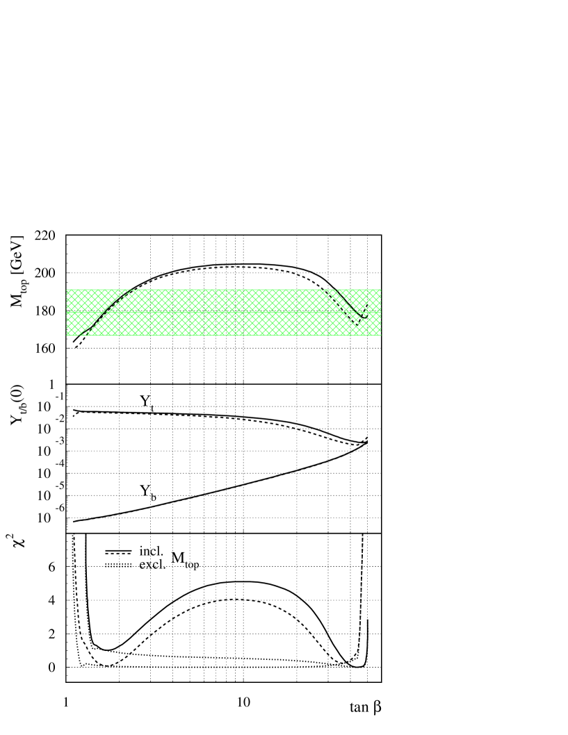
Figure 1: The top quark mass as function of ${\tan\beta}$ (top) for values of ${m_{0}},{m_{1/2}}$ optimized for low and high ${\tan\beta}$, as indicated by the dashed and solid lines, respectively. The middle part shows the corresponding values of the Yukawa coupling at the GUT scale and the lower part the obtained $\chi^{2}$ values. If the top constraint (${m_{t}}=179\pm 12$, horizontal band) is not applied, all values of ${\tan\beta}$ between 1.2 and 50 are allowed (thin dotted lines at the bottom), but if the top mass is constrained to the experimental value, only the regions $1<{\tan\beta}<3$ and $25<{\tan\beta}<50$ are allowed.

The requirement of $b-\tau$ Yukawa coupling unification strongly restricts the possible solutions in the $M_{t}$ versus ${\tan\beta}$ plane, as discussed before. With the top mass measured by the CDF and D0-Collaborations [39, 40] only two regions of ${\tan\beta}$ give an acceptable $\chi^{2}$ fit, as shown in the bottom part of fig. 1 for two values of the SUSY scales ${m_{0}},{m_{1/2}}$, which are optimized for the low and high ${\tan\beta}$ range, respectively, as will be discussed below. The curves at the top show the solution for $M_{t}$ as function of ${\tan\beta}$ in comparison with the experimental value of $M_{t}=179\pm 12$ GeV. The $M_{t}$ predictions were obtained by imposing gauge coupling unification and electroweak symmetry breaking for each value of ${\tan\beta}$, which allows a determination of $\mu,~{}{\alpha_{\rm GUT}}$, and ${M_{\rm GUT}}$ from the fit for the given choice of ${m_{0}},{m_{1/2}}$. The results do not depend very much on this choice, as can be seen from a comparison of the solid and dotted lines in fig. 1.

The best $\chi^{2}$ is obtained for ${\tan\beta}=1.7$ and ${\tan\beta}=42$, respectively. They correspond to solutions where $Y_{t}\gg Y_{b}$ and $Y_{t}\approx Y_{b}$, as shown in the middle part of fig. 1. The latter solution is the one typically expected for the SO(10) symmetry, in which the up and down type quarks as well as leptons belong to the same multiplet, while the first solution corresponds to $b-\tau$ unification only, as expected for the minimal SU(5) symmetry.

4.2 Electroweak symmetry breaking

Eq. (43) for ${M_{Z}}$ can be written as

$$\tan^{2}\beta = \frac{m_{1}^{2}+\Sigma_{1}+\frac{1}{2}M_{Z}^{2}}{m_{2}^{2}+\Sigma_{2}+\frac{1}{2}M_{Z}^{2}}.$$ (54)

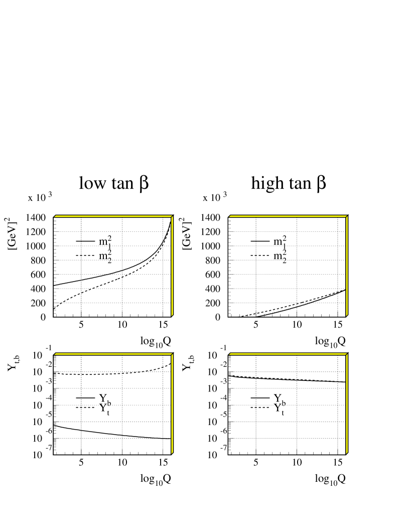
Figure 2: The running of the parameters $m_{1}$ and $m_{2}$ in the Higgs potential (top) and Yukawa couplings of top and bottom quarks (bottom).

From fig. 2 one observes that at low energy $m_{1}^{2}+\Sigma_{1}>m_{2}^{2}+\Sigma_{2}$ as expected, since $\Sigma_{2}$ ($\Sigma_{1}$) contains large negative corrections proportional to $Y_{t}$ ($Y_{b}$) and $Y_{t}\gg Y_{b}$. Consequently the numerator in eq. 54 is always larger than the denominator, implying $\tan^{2}\beta>1$.

For the large $\tan\beta$ scenario $Y_{t}\approx Y_{b}$, so $\Sigma_{1}\approx\Sigma_{2}$ (see fig. 2). Eq. 54 then requires the starting values of $m_{1}$ and $m_{2}$ to be different in order to obtain a large value of $\tan\beta$.

Several reasons for such a splitting could be thought of. E.g. SO(10) may be broken at a scale $M_{\rm SO(10)}$ above $M_{\rm GUT}$ but below ${M_{\rm Planck}}.$ Such a symmetry breaking can lead to a direct splitting between $m_{1}$ and $m_{2}$ [74, 75, 76]. In addition $Y_{t}$ and $Y_{b}$ may be different at $M_{\rm GUT}$ due to the evolution between $M_{\rm SO(10)}$ and $M_{\rm GUT}$ .

Using the RGE for the SU(5) group from ref. [77], we found $Y_{t}\approx 1.05Y_{b}$ and $m_{1}\approx 0.96m_{2}$ for the best fitted value of ${M_{\rm SO(10)}}\approx 6\cdot 10^{17}$ GeV. However these splittings are not large enough to generate electroweak symmetry breaking.

Good fits can be obtained by splittings between $m_{1}^{2}$ and $m_{2}^{2}$ and $Y_{t}$ and $Y_{b}$ of the order of 25%, which we used in the following analysis ($Y_{b}(0)=0.75Y_{t}(0)$, $m_{1}^{2}=1.25m_{0}^{2}+\mu^{2}$, $m_{2}^{2}=m_{0}^{2}+\mu^{2}$ at the GUT scale).

The Higgs mixing parameter $\mu$ can be determined from radiative electroweak symmetry breaking (EWSB), since eq. 43 can be rewritten as:

$$\mu^{2}=\frac{m^{2}_{H_{1}}-m^{2}_{H_{2}}\tan^{2}\beta}{\tan^{2}\beta-1}+\frac{\Sigma_{1}-\Sigma_{2}\tan^{2}\beta}{\tan^{2}\beta-1}-\frac{M_{Z}^{2}}{2}\;.$$ (55)

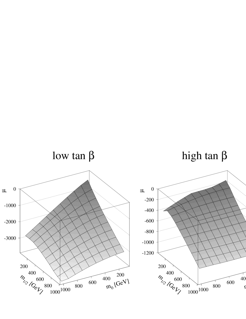
Figure 3: The Higgs mixing parameter $\mu_{0}$ at the GUT scale as function of ${m_{0}}$ and ${m_{1/2}}$ for the low and high ${\tan\beta}$ scenario, respectively.

The dependence of $\mu$ on $m_{0}$ and $m_{1/2}$ is shown in fig. 3. Due to the strong ${\tan\beta}$ dependence in eq. 55, the values are much smaller for the high ${\tan\beta}$ scenario. One observes that EWSB breaking determines only $\mu^{2}$, so the mixing in the stop sector can be either large or small, depending on the relative sign of $\mu$ and $A_{t}$.

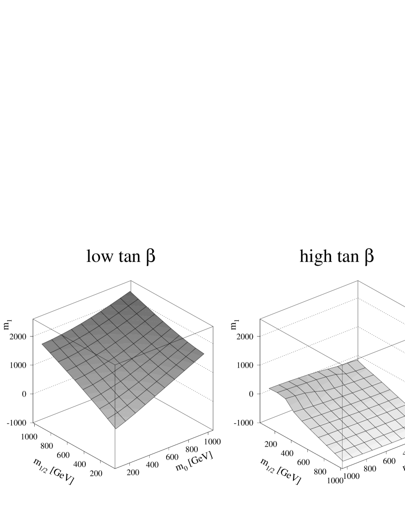
Figure 4: The mass $m_{1}$ in the Higgs potential at ${M_{Z}}$ (Born level) in GeV as function of ${m_{0}}$ and ${m_{1/2}}$ for the low and high ${\tan\beta}$ scenario, respectively.

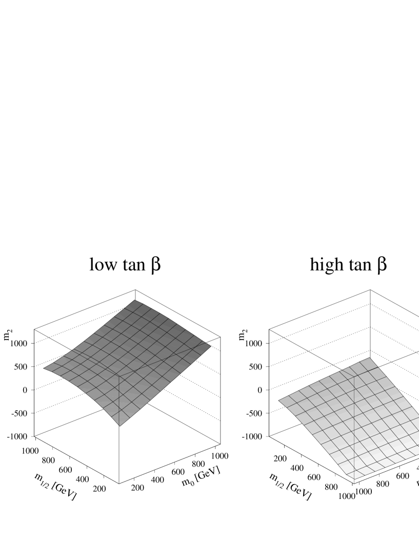
Figure 5: The mass $m_{2}$ in the Higgs potential at ${M_{Z}}$ (Born level) in GeV as function of ${m_{0}}$ and ${m_{1/2}}$ for the low and high ${\tan\beta}$ scenario, respectively.

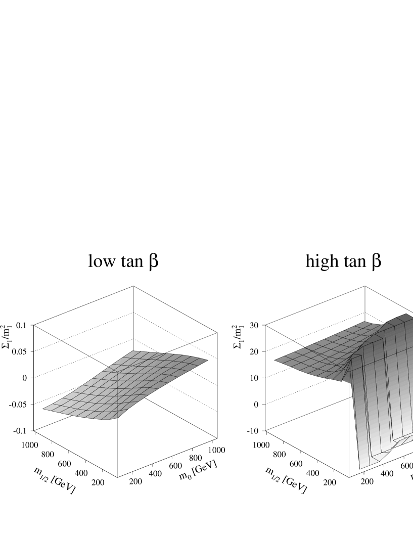
Figure 6: The one-loop corrections $\Sigma_{1}/m_{1}^{2}$ at ${M_{Z}}$ as function of ${m_{0}}$ and ${m_{1/2}}$ for the low and high ${\tan\beta}$ scenario, respectively.

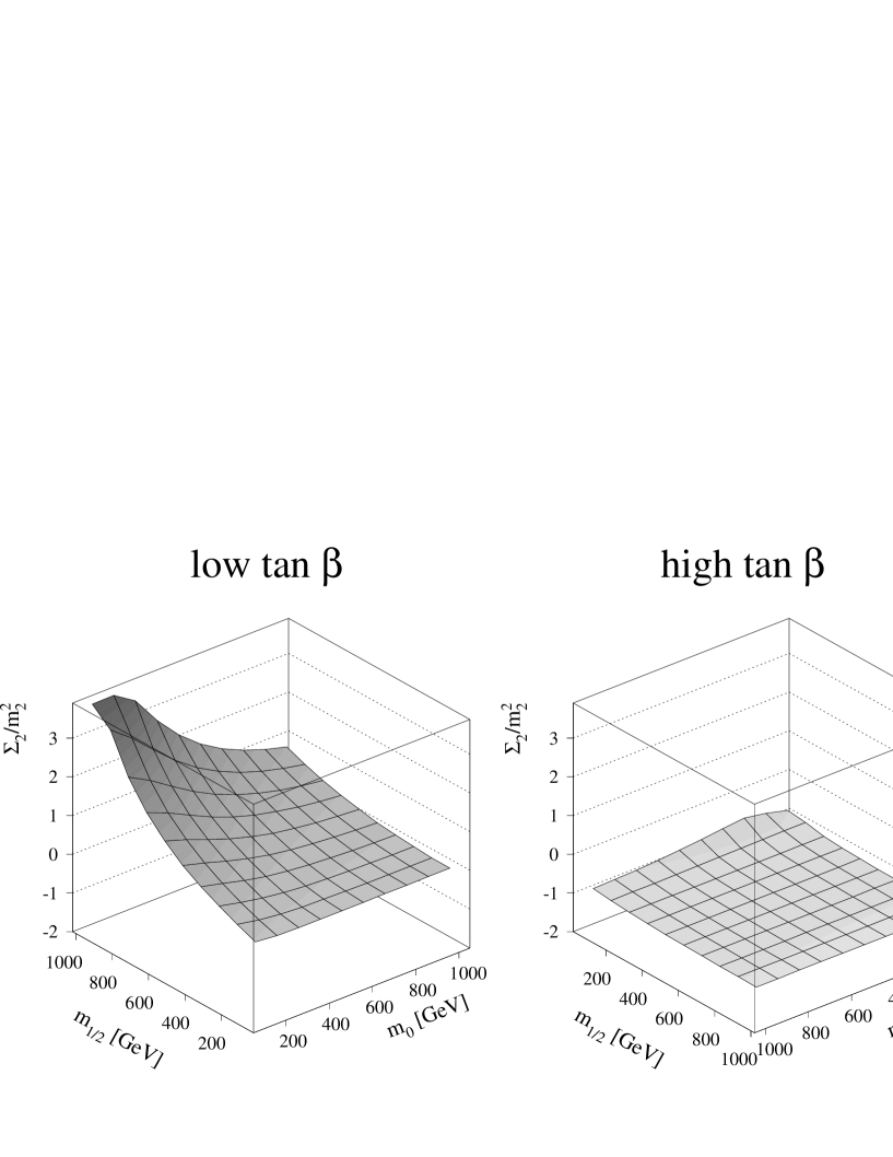
Figure 7: The one-loop corrections $\Sigma_{2}/m_{2}^{2}$ at ${M_{Z}}$ as function of ${m_{0}}$ and ${m_{1/2}}$ for the low and high ${\tan\beta}$ scenario, respectively.

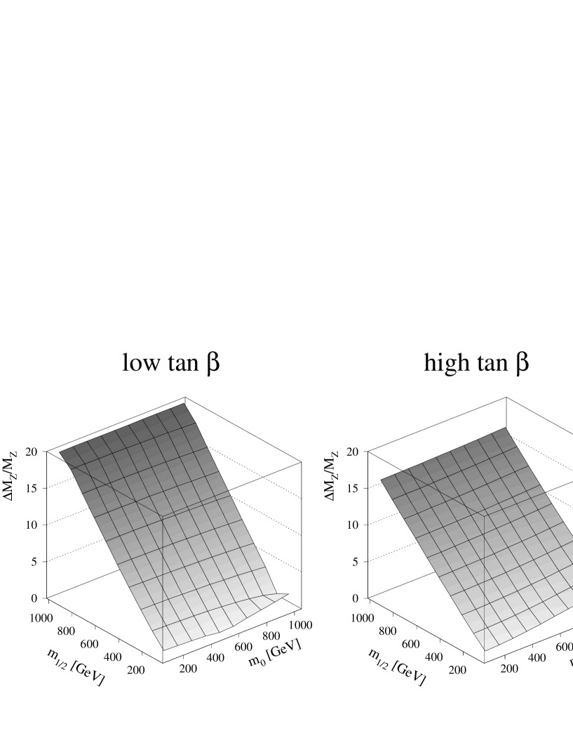
Figure 8: The one-loop radiative corrections $\Delta({M_{Z}})/{M_{Z}}$ as function of ${m_{0}}$ and ${m_{1/2}}$ for the low and high ${\tan\beta}$ scenario, respectively.

For large values of $m_{0}$ and $m_{1/2}$ the masses of the superpartners and the normal particles become different. In this case the famous cancellation of quadratic divergencies in supersymmetry does not work anymore, leading to large corrections for the Higgs potential parameters and electroweak scale, as shown in figs. 4-8. For clarity the Born terms have been displayed, too.

It is a question of taste if one should exclude the regions with large corrections. In our opinion such a fine tuning argument is difficult to use for a mass scale below 1 TeV, and the whole region up to 1 TeV should be considered, leading to quite large upper limits in case of the low ${\tan\beta}$ scenario[14].

4.3 Discussion of the remaining constraints

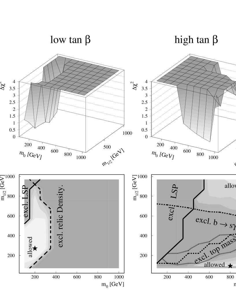
Figure 9: The total $\chi^{2}$-distribution for low and high ${\tan\beta}$ solutions (top) as well as the projections (bottom). The different shades indicate steps of $\Delta\chi^{2}=1$, so basically only the light region is allowed. The stars indicate the optimum solution.

In fig. 9 the total $\chi^{2}$ distribution is shown as a function of ${m_{0}}$ and ${m_{1/2}}$ for the two values of ${\tan\beta}$ determined above. One observes clear minima at ${m_{0}},{m_{1/2}}$ around (200,270) and (800,88), as indicated by the stars in the projections. The different shades correspond to $\Delta\chi^{2}$ steps of 1. Note the sharp increase in $\chi^{2}$, so basically only the light shaded regions are allowed independent of the exact $\chi^{2}$ cut. The fitted values of the other parameters are shown in table 2 and the corresponding SUSY masses are given in table 3.

The running of some masses down to $M_{Z}$ is shown in fig. 10. The values in table 3 are not the values at $M_{Z}$, but at the physical mass $m_{i}$ for each particle, since the running was stopped at $m_{i}$.

The contours in fig. 9 show the regions excluded by different constraints used in the analysis, as will be discussed below.

• LSP Constraint: The requirement that the LSP is neutral excludes the regions with small $m_{0}$ and relatively large $m_{1/2}$, since in this case one of the scalar staus becomes the LSP after mixing via the off-diagonal elements in the mass matrix (eq. 2.2). The LSP constraint is especially effective at the high $\tan\beta$ region, since the off-diagonal element is proportional to $A_{t}m_{0}-\mu\tan\beta$.

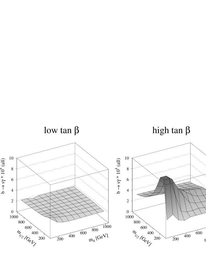
Figure 11: The branching ratio $b\rightarrow s\gamma$ as function of ${m_{0}}$ and ${m_{1/2}}$. Note that for large $\tan\beta$  only the region for ${m_{1/2}}<120$ GeV yields values compatible with experimental results.

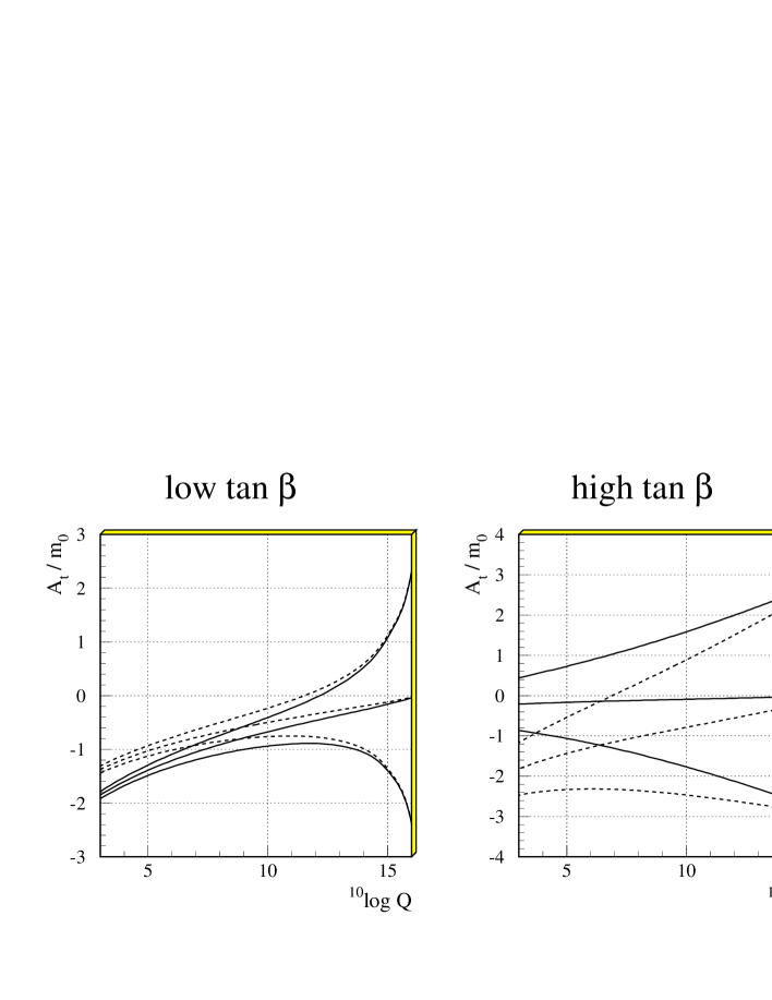
Figure 12: The running of $A_{t}$. The values of (${m_{0}},{m_{1/2}}$) were chosen to be (200,270) and (800,88) GeV for the low and high ${\tan\beta}$ scenario, respectively. However, the fixed point behaviour is found for other values of ${m_{0}},{m_{1/2}}$ too: at low values of ${\tan\beta}$ a strong convergence to a single value is found, while for high values this tendency is much less pronounced.

• $b\rightarrow s\gamma$ Rate: The predicted $b\rightarrow s\gamma$ rate is shown in fig. 11 as function of $m_{0}$ and $m_{1/2}$ (with all other parameters optimized by the fit). At low $\tan\beta$ the $b\rightarrow s\gamma$ rate is close to its SM value for most of the plane. The charginos and/or the charged Higgses are only light enough at small values of $m_{0}$ and $m_{1/2}$ to contribute significantly. The trilinear couplings were found to play a negligible role for low $\tan\beta$ . Varying them between $\pm 3{m_{0}}$ did not change the results significantly, since $A_{t}$ shows a fixed point behaviour in this case: its value at ${M_{Z}}$ is practically independent of the starting value at the GUT scale, as shown in fig. 12.

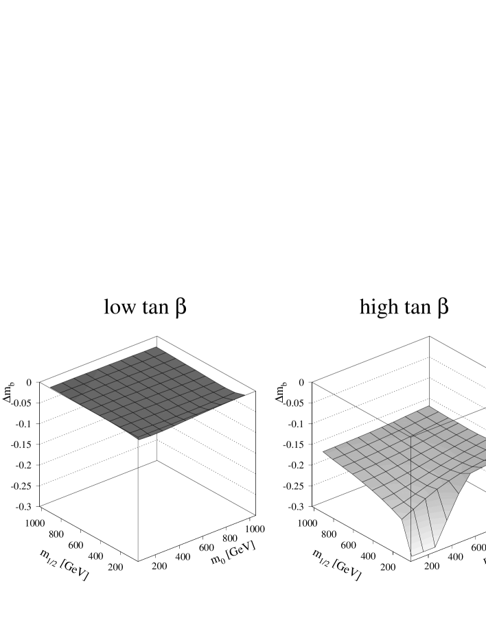
Figure 13: Corrections to the bottom quark mass from gluino, charged Higgses and Higgsino loop contributions in the MSSM as function of ${m_{0}}$ and ${m_{1/2}}$. Note the large negative corrections for $|\mu|<0$ in this case. Positive $\mu$-values would yield a large positive contribution, which excludes bottom-$\tau$ unification for most of the parameter space.

  However, for large ${\tan\beta}$ the trilinear coupling needs to be left free, since it is difficult to fit simultaneously ${b\rightarrow s\gamma}$, $m_{b}$ and $m_{\tau}$. The reason is that the corrections to $m_{b}$ are large for large values of $\tan\beta$ due to the large contributions from $\tilde{g}-\tilde{q}$ and $\tilde{\chi}^{\pm}-\tilde{t}$ loops proportional to $\mu{\tan\beta}$ (see eq. 44). They become of the order of 10-20%, as shown in fig. 13. In order to obtain $m_{b}(M_{Z})$ as low as 2.84 GeV, these corrections have to be negative, thus requiring $\mu$ to be negative.

  As shown in fig. 11 the $b\rightarrow s\gamma$ rate is too large in most of the parameter region for large $\tan\beta$ . In order to reduce this rate one needs $A_{t}(M_{Z})>0$ for $\mu<0$ (see eq. 51). Since for large $\tan\beta$ $A_{t}$ does not show a fix point behaviour (see fig. 12), this is possible. The $\chi^{2}$ for large ${\tan\beta}$ and $A_{0}=0$ is much worse than for fits in which $A_{0}$ is left free, as can be seen in fig. 14; also the influence of $\Delta m_{b}$ on the $b-\tau$ unification solution is shown on the left side. Note that the $\Delta m_{b}$ corrections improve the fit.

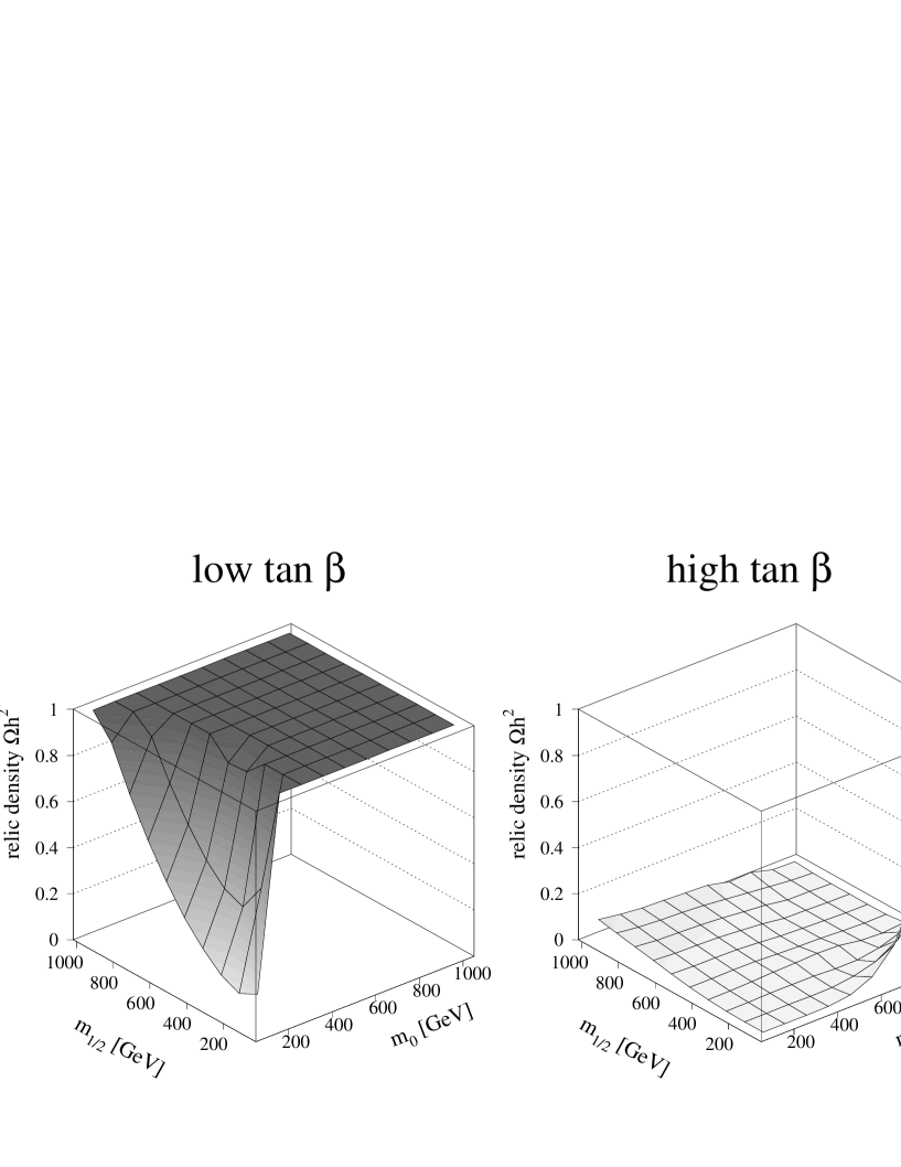
Figure 15: The relic density as function of ${m_{0}}$ and ${m_{1/2}}$ for the low and high ${\tan\beta}$ scenario, respectively.

• Relic Density: the predicted Relic Density is shown in fig. 15. For the low $\tan\beta$ scenario the value of $\mu$ from EWSB is large (see fig. 3). In this case there is little mixing between the Higgsino and Gaugino sector as is apparent from the neutralino mass matrix: for $|\mu|\gg M_{1}\approx 0.4m_{1/2}$ the mass of the LSP is simply $0.4m_{1/2}$ and the “bino” purity is 99% (see table 2). For the high $\tan\beta$ scenario $\mu$ is much smaller (see fig. 3) and the Higgsino admixture becomes larger. This leads to an enhancement of $\tilde{\chi}-\tilde{\chi}$ annihilation via the s-channel Z boson exchange, thus reducing the relic density. As a result, in the large ${\tan\beta}$ case the constraint $\Omega h_{0}^{2}<1$ is almost always satisfied unlike in the case of low ${\tan\beta}$.

The mass of the lightest chargino is about $0.7~{}-0.8~{}{m_{1/2}}$, as shown in fig. 16. The low value of ${m_{1/2}}$ for the best fit at large ${\tan\beta}$ is mainly restricted by the chargino mass limit of $65GeV$ included in the fit. However, it will be difficult to exclude the large ${\tan\beta}$ scenario, since a change of the limit on the chargino masses from 65 GeV to the possible limit of 95 GeV at LEPII does not significantly change the $\chi^{2}$ of the best fit.

Of course, this conclusion depends sensitively on the $BR(b\rightarrow s\gamma)$ value. For large ${m_{1/2}}$ values, the prediction for this branching ratio is only 2 or 3 standard deviations above its experimental value (see fig. 11).

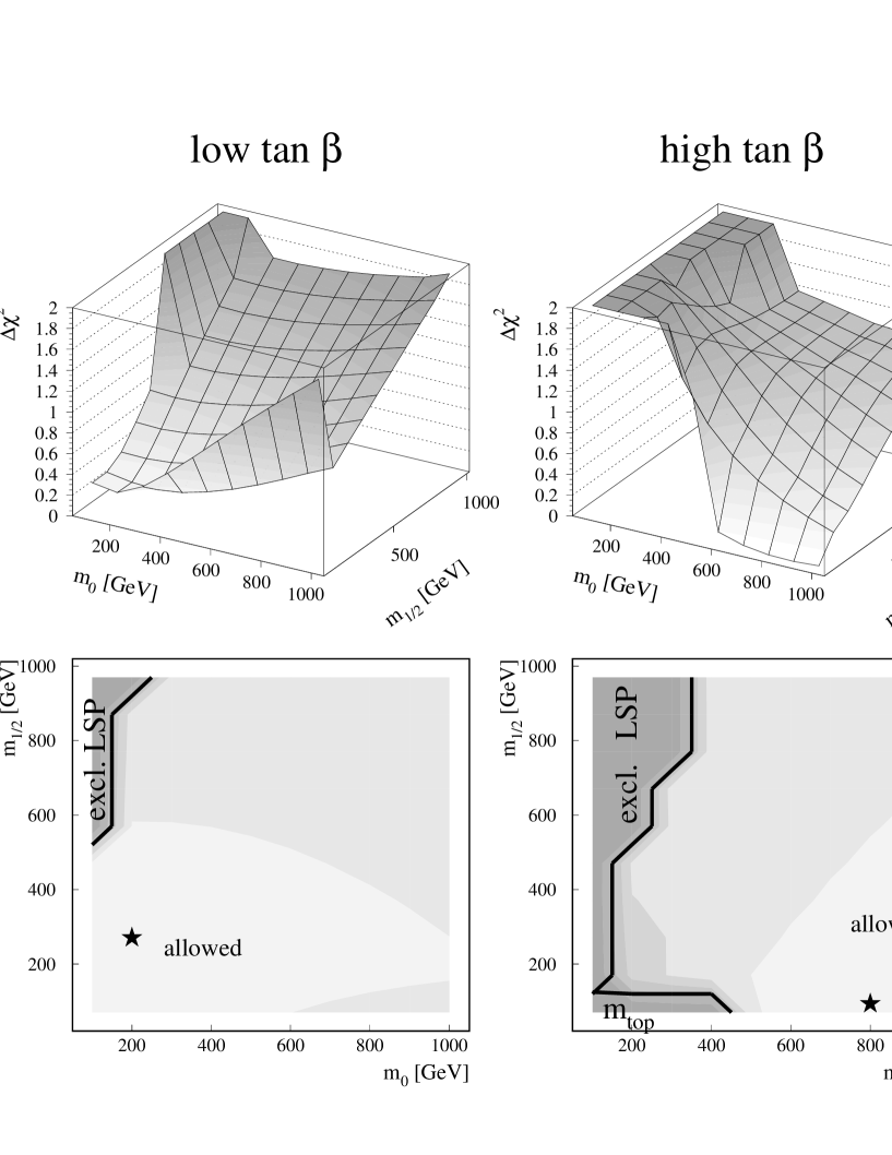
Figure 17: As fig. 9, but only including the constraints from unification and electroweak symmetry breaking.

Without the constraints from $b\rightarrow s\gamma$ and dark matter, large values of the SUSY scale cannot be excluded, since the $\chi^{2}$ from gauge and Yukawa coupling unification and electroweak symmetry breaking alone does not exclude these regions (see fig. 17). However, there is a clear preference for the lighter SUSY scales.

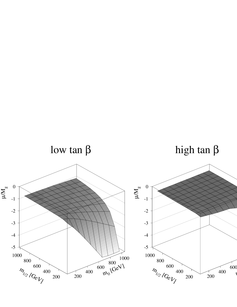
Figure 18: The ratio of $\mu({M_{Z}})$ and the gluino mass as function of ${m_{0}}$ and ${m_{1/2}}$ for the low and high ${\tan\beta}$ scenario, respectively.

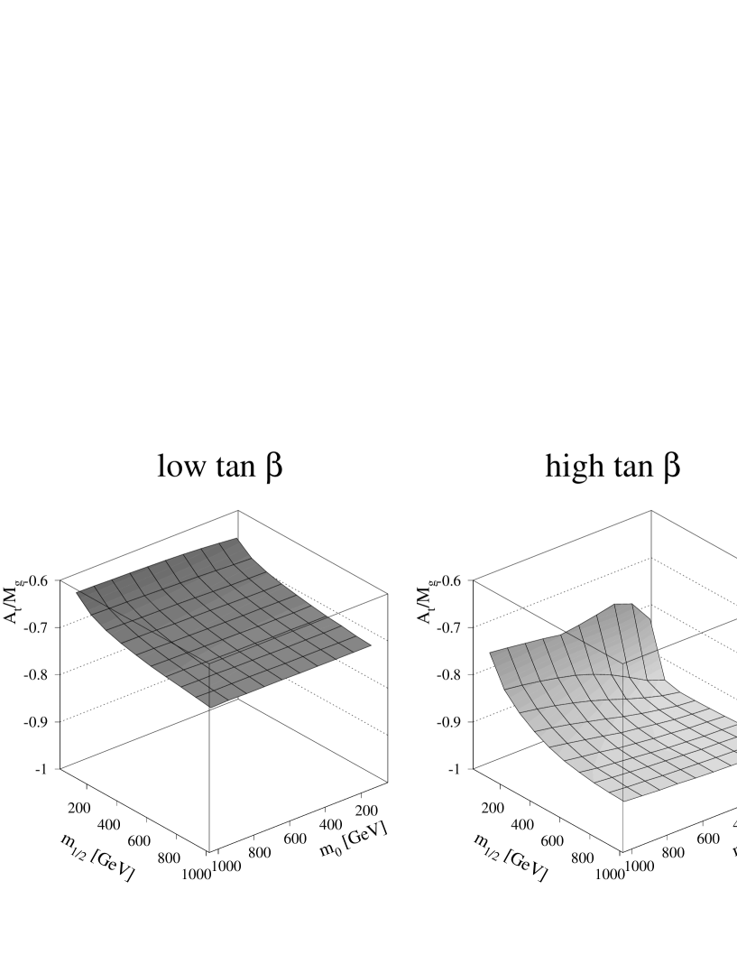
Figure 19: The ratio of $A_{t}$ and the gluino mass as function of ${m_{0}}$ and ${m_{1/2}}$ for the low and high ${\tan\beta}$ scenario, respectively ($A_{0}=0$).

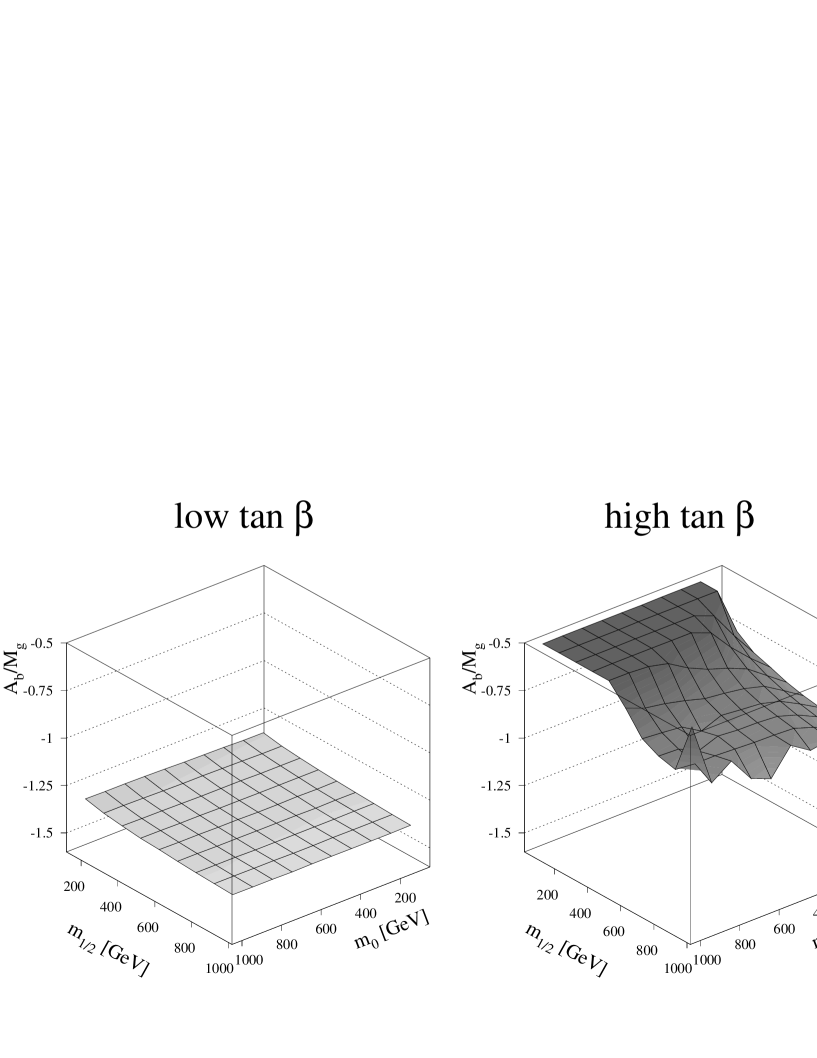
Figure 20: The ratio of $A_{b}({M_{Z}})$ and the gluino mass as function of ${m_{0}}$ and ${m_{1/2}}$ for the low and high ${\tan\beta}$ scenario, respectively ($A_{0}=0$).

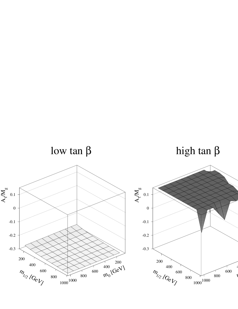
Figure 21: The ratio of $A_{\tau}({M_{Z}})$ and the gluino mass as function of ${m_{0}}$ and ${m_{1/2}}$ for the low and high ${\tan\beta}$ scenario, respectively ($A_{0}=0$).

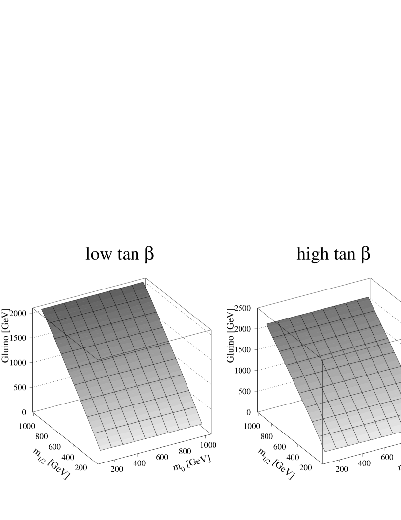
Figure 22: The gluino mass as function of ${m_{0}}$ and ${m_{1/2}}$ for the low and high ${\tan\beta}$ scenario, respectively.

The fitted values of the trilinear couplings and the Higgs mixing parameter $\mu$ are strongly correlated with ${m_{1/2}}$, so the ratio of these parameters at the electroweak scale and the gluino mass is relatively constant and largely independent of ${m_{0}}$ (see figs. 18 - 21). The gluino mass depends only on $m_{1/2}$ ($M_{\tilde{g}}\approx 2.7~{}{m_{1/2}}$), as shown in fig. 22. Note from the figures that although the trilinear couplings $A_{t}$, $A_{b}$ and $A_{\tau}$ have equal values at the GUT scale, they are quite different at the electroweak scale due to the different radiative corrections.

5 Discovery Potential at LEP II

Table 3 shows that charginos, neutralinos and the lightest Higgs belong to the lightest particles in the MSSM.

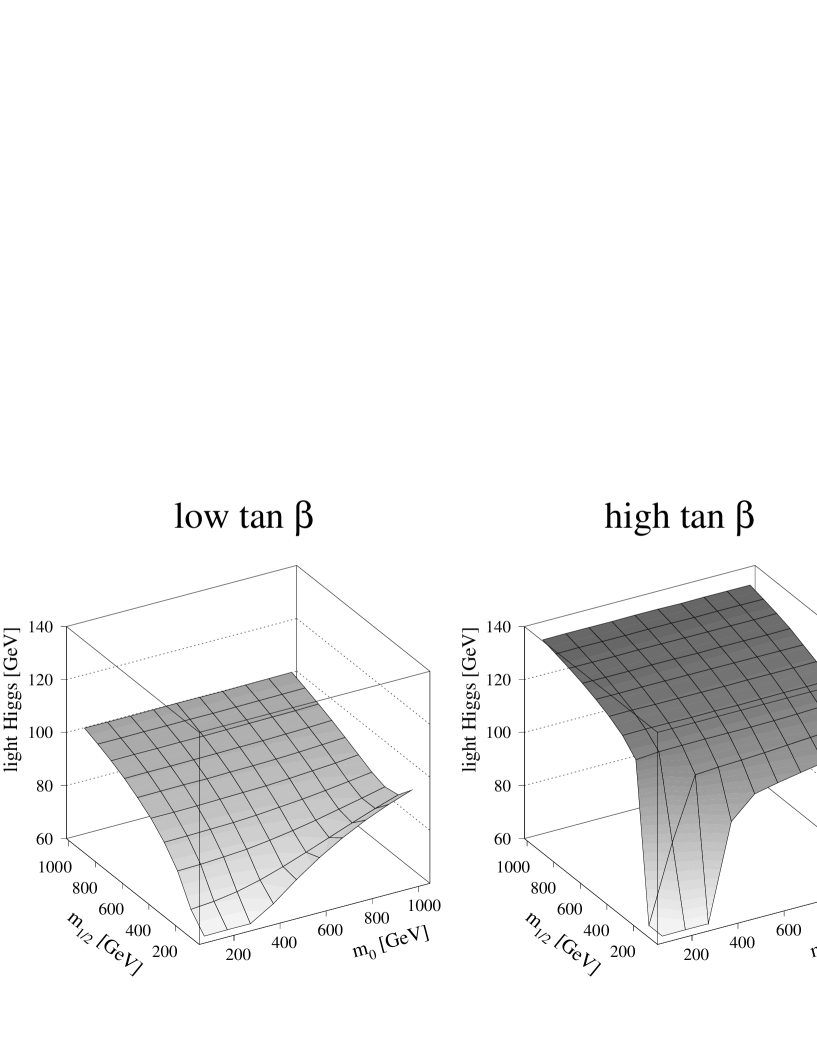
Figure 23: The mass of the lightest CP-even Higgs as function of ${m_{0}}$ and ${m_{1/2}}$ for the low and high ${\tan\beta}$ scenario, respectively. The sign of $\mu$ is negative, as required for the high ${\tan\beta}$ solution, but chosen negative for low ${\tan\beta}$.

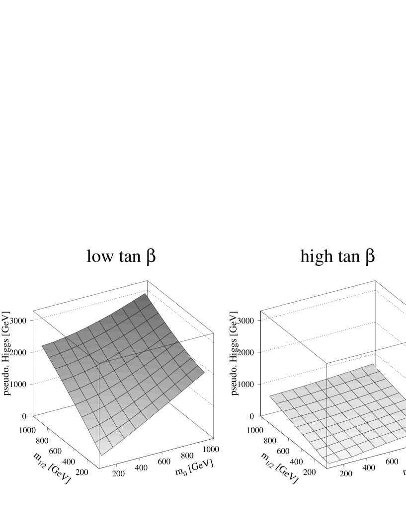
Figure 24: The mass of the CP-odd Higgs as function of ${m_{0}}$ and ${m_{1/2}}$ for the low and high ${\tan\beta}$ scenario, respectively.

In figs. 23,24 the masses of the lightest CP-even and CP-odd Higgs bosons are shown for the whole parameter space for negative $\mu$-values. At each point a fit was performed to obtain the best solution for the GUT parameters. The mass of the lightest Higgs saturates at 100 GeV. For positive $\mu$-values and low ${\tan\beta}$ the maximum Higgs mass increases to 115 GeV.

For high ${\tan\beta}$ only negative $\mu$-values are allowed, since positive $\mu$-values yield a too high $b$-mass due to the large positive corrections in that case, as discussed above.

The programs SUSYGEN [78] and special SUSY routines [79] in ISAJET [80] have been used to calculate the production cross sections.

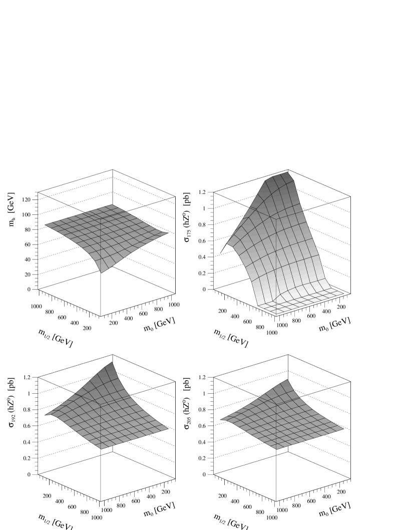
Figure 25: The Higgs mass as function of ${m_{0}}$ and ${m_{1/2}}$ for positive values of $\mu$ and ${\tan\beta}=1.7$ (left top corner) and the main production cross sections for three different LEP II energies (175, 192 and 205 GeV). For negative $\mu$-values the cross sections are about 50% larger.

Fig. 25 shows the mass of the lightest Higgs boson and the corresponding Higgs production cross sections at three LEP energies as functions of $m_{0}$ and $m_{1/2}$ for $\tan\beta=1.7$ and $m_{t}=180$ GeV.

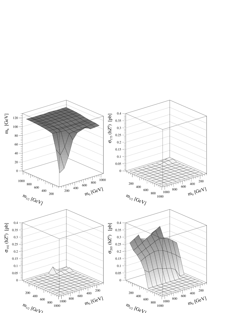
Figure 26: The Higgs mass as function of ${m_{0}}$ and ${m_{1/2}}$ for $\mu=-300$ GeV and ${\tan\beta}=46$ (left top corner) and the main production cross sections for three different LEP II energies (175, 192 and 205 GeV).

Here the most significant second order corrections to the Higgs mass have been incorporated [81], which reduces the Higgs mass by about 15 GeV [30]. In this case the foreseen LEP energy of 192 GeV is sufficient to cover the whole parameter space for the low $\tan\beta$ scenario, provided the top mass is below 190 GeV. For the large $\tan\beta$ scenario one needs the maximum possible LEP II energy of 205 GeV in order to cover at least some part of the parameter space, as shown in fig. 26.

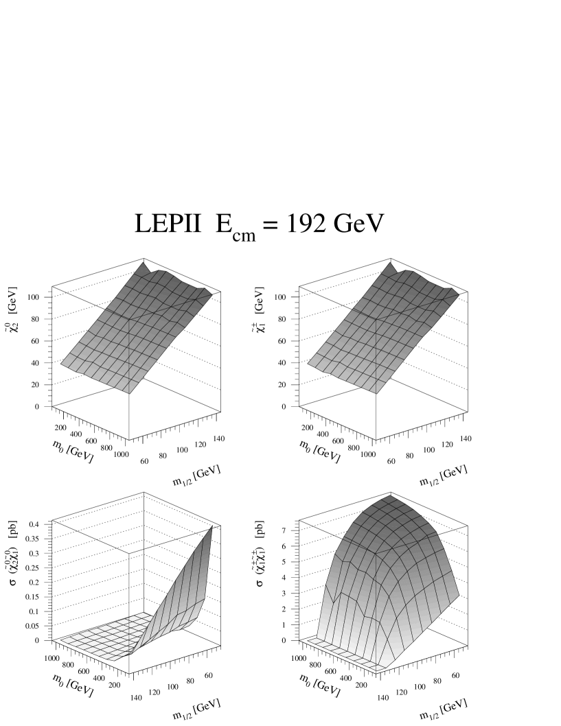
Figure 28: The masses of the second lightest neutralino and chargino masses as well as the production cross sections for $\mu=-300$ GeV and ${\tan\beta}=46$. $\mu$ was kept to a representative value, since in most of the region the fit gave an unacceptable $\chi^{2}$, so $\mu$ could not be determined. Positive values of $\mu$ give similar results. The steep decrease in the chargino cross section at small values of ${m_{0}}$ is due to the light sneutrino, which leads to a strong negative interference between s- and t-channel in that case. Fortunately, the neutralino production is large in that region,as shown by the plot in the left bottom corner.

The cross section dependence on the centre of mass energy is shown for some representative Higgs masses in fig 27. Clearly the large $\tan\beta$ scenario is not very promising for the Higss mass discovery at LEP II. However, in that case the discovery potential of the chargino and neutralino searches is high, since the cross sections are large for $m_{1/2}<120$ GeV, as shown in fig. 28. This is exactly the region allowed by all other constraints for large $\tan\beta$ (see fig. 9), if one ignores the other solution with $m_{\tilde{q}}\geq 3$ TeV, i.e. $m_{1/2}\approx m_{0}\approx 1$ TeV.

6 Summary

In the Constrained Minimal Supersymmetric Model (CMSSM) the optimum values of the GUT scale parameters and the corresponding SUSY mass spectra for the low and high ${\tan\beta}$ scenario have been determined from a combined fit to the low energy data on couplings, quark and lepton masses of the third generation, the electroweak scale ${M_{Z}}$, ${b\rightarrow s\gamma}$, and the lifetime of the universe.

The solutions preferred by the best fit predict new particles at LEP II: The lightest Higgs boson in case of the low $\tan\beta$ scenario and chargino or neutralino production at the high $\tan\beta$ scenario. The upper limits on the masses of these particles are outside the LEP II domain, but within reach of the LHC.

7 Acknowledgement

The research described in this publication was made possible in part by support from the Human Capital and Mobility Fund (Contract ERBCHRXCT 930345) from the European Community, and by support from the German Bundesministerium für Bildung und Forschung (BMBF) (Contract 05-6KA16P) and from the Deutsche Forschungs-Gemeinschaft (DFG) for the Graduiertenkolleg in Karlsruhe.

Fitted SUSY parameters
Symbol	low ${\tan\beta}$	high ${\tan\beta}$
$m_{0}$	200	800
$m_{1/2}$	270	88
$\mu(0)$	-1084	-270
$\mu({M_{Z}})$	-546	-220
$\tan\beta$	1.71	41.2
$Y_{t}({m_{t}})$	0.0080	0.0051
$Y_{t}(0)$	0.0416	0.0014
$Y_{b}(0)$	0.12E-05	0.0011
$M_{t}^{pole}$	177	165
$m_{t}^{running}$	168	157
$1/\alpha_{\rm GUT}$	24.8	24.3
${M_{\rm GUT}}$	$1.6\;10^{16}$	$2.5\;10^{16}$
$A(0)m_{0}$	0	1256
$A_{t}({M_{Z}})m_{0}$	-446	149
$A_{b}({M_{Z}})m_{0}$	-886	190
$A_{\tau}({M_{Z}})m_{0}$	-182	639
$m_{1}({M_{Z}})m_{0}$	612	207
$m_{2}({M_{Z}})m_{0}$	262	-180

Table 2: Values of the fitted SUSY parameters for low and high ${\tan\beta}$ (in GeV, when applicable). The scale is either ${M_{Z}}$, ${m_{t}}$, or ${\rm GUT}$, as indicated in the first column by (${M_{Z}}$), (${m_{t}}$) or (0), respectively. The SUSY mass spectrum corresponding to these parameters is given in table 3.

SUSY masses in [GeV]
Symbol	low ${\tan\beta}$	high ${\tan\beta}$
$\tilde{\chi}^{0}_{1}(\tilde{B})$	116	35
$\tilde{\chi}^{0}_{2}(\tilde{W}^{3})$	231	65
$\tilde{\chi}^{\pm}_{1}(\tilde{W}^{\pm})$	231	65
$\tilde{g}$	658	236
$\tilde{e}_{L}$	278	804
$\tilde{e}_{R}$	228	802
$\tilde{\nu}_{L}$	273	799
$\tilde{q}_{L}$	628	825
$\tilde{q}_{R}$	605	823
$\tilde{\tau}_{1}$	227	557
$\tilde{\tau}_{2}$	228	695
$\tilde{b}_{1}$	560	463
$\tilde{b}_{2}$	604	549
$\tilde{t}_{1}$	477	461
$\tilde{t}_{2}$	582	543
$\tilde{\chi}^{0}_{3}(\tilde{H}_{1})$	562	(-)240
$\tilde{\chi}^{0}_{4}(\tilde{H}_{2})$	(-)571	248
$\tilde{\chi}^{\pm}_{2}(\tilde{H}^{\pm})$	569	254
$h$	81	110
$H$	739	273
$A$	734	273
$H^{\pm}$	738	285
$\Omega h^{2}$	0.42	0.19
Br($b\rightarrow s\gamma$ )	$2.87\;10^{-4}$	$2.5\;10^{-4}$
LSP$\rightarrow|\tilde{B}>$	0.9973	0.97
LSP$\rightarrow|\tilde{W}^{3}>$	0.0360	-0.05
LSP$\rightarrow|\tilde{H}_{1}^{0}>$	-0.0593	-0.22
LSP$\rightarrow|\tilde{H}_{2}^{0}>$	0.0252	-0.03

Table 3: Values of the SUSY mass spectra for the low and high ${\tan\beta}$ solutions, given in table 2. The (-) in front of the neutralinos indicates that it is a CP-odd state. The LSP is a linear combination of the gaugino and Higgsino components, as indicated by the last four rows. Note the much larger Higgsino component of the LSP for large ${\tan\beta}$, which leads to a small relic density.

$$\begin{array}[]{|c|c|c|c|}\hline\cr\mbox{Particle}&b_{1}&b_{2}&b_{3}\\ \hline\cr\hline\cr\rule{0.0pt}{14.22636pt}\tilde{g}&0&0&2\\ \rule{0.0pt}{14.22636pt}\tilde{l}_{l}&\frac{3}{10}&\frac{1}{2}&0\\ \rule{0.0pt}{14.22636pt}\tilde{l}_{r}&\frac{3}{5}&0&0\\ \rule{0.0pt}{14.22636pt}\tilde{w}&0&\frac{4}{3}&0\\ \rule{0.0pt}{14.22636pt}\tilde{q}-\tilde{t}&\frac{49}{60}&1&\frac{5}{3}\\ \rule{0.0pt}{14.22636pt}\tilde{t}_{l}&\frac{1}{60}&\frac{1}{2}&\frac{1}{6}\\ \rule{0.0pt}{14.22636pt}\tilde{t}_{r}&\frac{4}{15}&0&\frac{1}{6}\\ \rule{0.0pt}{14.22636pt}\tilde{h}&\frac{2}{5}&\frac{2}{3}&0\\ \rule{0.0pt}{14.22636pt}H&\frac{1}{10}&\frac{1}{6}&0\\ \rule{0.0pt}{14.22636pt}t&\frac{17}{30}&1&\frac{2}{3}\\ &&&\\ \hline\cr&&&\\ \rule{0.0pt}{14.22636pt}\mbox{SM}&\frac{41}{10}&-\frac{19}{6}&-7\\ \rule{0.0pt}{14.22636pt}\mbox{MSSM}&\frac{33}{5}&1&-3\\ &&&\\ \hline\cr\end{array}$$

Table 4: First order contributions to RG-equations.

$$\begin{array}[]{|c|c|}\hline\cr\mbox{Particle}&b_{ij}\\ \hline\cr\hline\cr\tilde{g}&\left(\begin{array}[]{rrr}\rule{0.0pt}{14.22636pt}0&0&0\\ \rule{0.0pt}{14.22636pt}0&0&0\\ \rule{0.0pt}{14.22636pt}0&0&48\end{array}\right)\\ \hline\cr\tilde{w}&\left(\begin{array}[]{rrr}\rule{0.0pt}{14.22636pt}0&0&0\\ \rule{0.0pt}{14.22636pt}0&\frac{64}{3}&0\\ \rule{0.0pt}{14.22636pt}0&0&0\end{array}\right)\\ \hline\cr\tilde{q},\tilde{l},\mbox{gauginos}&\left(\begin{array}[]{rrr}\rule{0.0pt}{14.22636pt}\frac{19}{15}&\frac{3}{5}&\frac{44}{15}\\ \rule{0.0pt}{14.22636pt}\frac{1}{5}&-\frac{7}{3}&4\\ \rule{0.0pt}{14.22636pt}\frac{11}{30}&\frac{3}{2}&-\frac{8}{3}\end{array}\right)\\ \hline\cr\begin{array}[]{l}\mbox{Heavy Higgses}\\ \mbox{and Higgsinos}\end{array}&\left(\begin{array}[]{rrr}\rule{0.0pt}{14.22636pt}\frac{9}{50}&\frac{9}{10}&0\\ \rule{0.0pt}{14.22636pt}\frac{3}{10}&\frac{29}{6}&0\\ \rule{0.0pt}{14.22636pt}0&0&0\end{array}\right)\\ \hline\cr\end{array}$$

Table 5: Second order contributions to RG-equations.

Region I		$\bf c^{t}_{ij}$
MSSM	$\bf c^{t}_{i}$	${\tilde{\alpha}}_{1}$	${\tilde{\alpha}}_{2}$	${\tilde{\alpha}}_{3}$	$Y_{t}$	$Y_{b}$	$Y_{\tau}$
${\tilde{\alpha}}_{1}$	$\frac{13}{15}$	$-\frac{2743}{450}$	$-1$	$-\frac{136}{45}$	$-\frac{6}{5}$	$-\frac{2}{5}$	$0$
${\tilde{\alpha}}_{2}$	$3$		$-\frac{15}{2}$	$-8$	$-6$	$0$	$0$
${\tilde{\alpha}}_{3}$	$\frac{16}{3}$			$\frac{16}{9}$	$-16$	$0$	$0$
$Y_{t}$	$-6$				$22$	$5$	$0$
$Y_{b}$	$-1$					$5$	$1$
$Y_{\tau}$	$0$						$0$
Region II
SM
${\tilde{\alpha}}_{1}$	$\frac{17}{20}$	$-\frac{1187}{600}$	$\frac{9}{20}$	$-\frac{19}{15}$	$-\frac{393}{80}$	$-\frac{7}{80}$	$-\frac{45}{24}$
${\tilde{\alpha}}_{2}$	$\frac{9}{4}$		$\frac{23}{4}$	$-9$	$-\frac{225}{16}$	$-\frac{99}{16}$	$-\frac{45}{24}$
${\tilde{\alpha}}_{3}$	$8$			$108$	$-36$	$-4$	$0$
$Y_{t}$	$-\frac{9}{2}$				$12$	$\frac{11}{4}$	$\frac{9}{4}$
$Y_{b}$	$-\frac{3}{2}$					$\frac{1}{4}$	$-\frac{5}{4}$
$Y_{\tau}$	$-1$						$\frac{9}{4}$

Table 6: One- and two-loop coefficients $c^{t}_{i}$ and $c^{t}_{ij}$ in the RG-equations.

Region I		$\bf c^{b}_{ij}$
MSSM	$\bf c^{b}_{i}$	${\tilde{\alpha}}_{1}$	${\tilde{\alpha}}_{2}$	${\tilde{\alpha}}_{3}$	$Y_{t}$	$Y_{b}$	$Y_{\tau}$
${\tilde{\alpha}}_{1}$	$\frac{7}{15}$	$-\frac{287}{90}$	$-1$	$-\frac{8}{9}$	$-\frac{4}{5}$	$-\frac{2}{5}$	$-\frac{6}{5}$
${\tilde{\alpha}}_{2}$	$3$		$-\frac{15}{2}$	$-8$	$0$	$-6$	$0$
${\tilde{\alpha}}_{3}$	$\frac{16}{3}$			$\frac{16}{9}$	$0$	$-16$	$0$
$Y_{t}$	$-1$				$5$	$5$	$0$
$Y_{b}$	$-6$					$22$	$3$
$Y_{\tau}$	$-1$						$3$
Region II
SM
${\tilde{\alpha}}_{1}$	$\frac{1}{4}$	$-\frac{127}{600}$	$\frac{27}{20}$	$-\frac{31}{15}$	$-\frac{91}{80}$	$-\frac{237}{80}$	$-\frac{15}{8}$
${\tilde{\alpha}}_{2}$	$\frac{9}{4}$		$\frac{23}{4}$	$-9$	$-\frac{99}{16}$	$-\frac{225}{16}$	$-\frac{15}{8}$
${\tilde{\alpha}}_{3}$	$8$			$108$	$-4$	$-36$	$0$
$Y_{t}$	$-\frac{3}{2}$				$\frac{1}{4}$	$\frac{11}{4}$	$-\frac{5}{4}$
$Y_{b}$	$-\frac{9}{2}$					$12$	$\frac{9}{4}$
$Y_{\tau}$	$-1$						$\frac{9}{4}$
Region III
SM - Top
${\tilde{\alpha}}_{1}$	$\frac{1}{4}$	$-\frac{127}{600}$	$\frac{27}{20}$	$-\frac{31}{15}$	$0$	$-\frac{237}{80}$	$-\frac{15}{8}$
${\tilde{\alpha}}_{2}$	$\frac{9}{4}$		$\frac{23}{4}$	$-9$	$0$	$-\frac{225}{16}$	$-\frac{15}{8}$
${\tilde{\alpha}}_{3}$	$8$			$108$	$0$	$-36$	$0$
$Y_{t}$	$0$				$0$	$0$	$0$
$Y_{b}$	$-\frac{9}{2}$					$12$	$\frac{9}{4}$
$Y_{\tau}$	$-1$						$\frac{9}{4}$

Table 7: One- and two-loop coefficients $c^{b}_{i}$ and $c^{b}_{ij}$. The coefficients are given for three integration regions: $M_{\rm SUSY}<Q<M_{\rm GUT}$ (MSSM), $m_{t}<Q<M_{\rm SUSY}$ (SM) and $M_{Z}<Q<m_{t}$ (SM – Top). Below the top mass all coefficients $c^{b}_{i}$ and $c^{b}_{ij}$ proportional to $Y_{t}$ have to be set to zero.

Region I		$\bf c^{\tau}_{ij}$
MSSM	$\bf c^{\tau}_{i}$	${\tilde{\alpha}}_{1}$	${\tilde{\alpha}}_{2}$	${\tilde{\alpha}}_{3}$	$Y_{t}$	$Y_{b}$	$Y_{\tau}$
${\tilde{\alpha}}_{1}$	$\frac{9}{5}$	$-\frac{27}{2}$	$-\frac{9}{5}$	$0$	$0$	$\frac{2}{5}$	$-\frac{6}{5}$
${\tilde{\alpha}}_{2}$	$3$		$-\frac{15}{2}$	$0$	$0$	$0$	$-6$
${\tilde{\alpha}}_{3}$	$0$			$0$	$0$	$-16$	$0$
$Y_{t}$	$0$				$0$	$3$	$0$
$Y_{b}$	$-3$					$9$	$9$
$Y_{\tau}$	$-4$						$10$
Region II
SM
${\tilde{\alpha}}_{1}$	$\frac{9}{4}$	$-\frac{1371}{200}$	$-\frac{27}{20}$	$0$	$-\frac{17}{8}$	$-\frac{5}{8}$	$-\frac{537}{80}$
${\tilde{\alpha}}_{2}$	$\frac{9}{4}$		$\frac{23}{4}$	$0$	$-\frac{45}{8}$	$-\frac{45}{8}$	$-\frac{165}{16}$
${\tilde{\alpha}}_{3}$	$0$			$0$	$-20$	$-20$	$0$
$Y_{t}$	$-3$				$\frac{27}{4}$	$-\frac{3}{2}$	$\frac{27}{4}$
$Y_{b}$	$-3$					$\frac{27}{4}$	$\frac{27}{4}$
$Y_{\tau}$	$-\frac{5}{2}$						$3$
Region III
SM - Top
${\tilde{\alpha}}_{1}$	$\frac{9}{4}$	$-\frac{1371}{200}$	$-\frac{27}{20}$	$0$	$0$	$-\frac{5}{8}$	$-\frac{537}{80}$
${\tilde{\alpha}}_{2}$	$\frac{9}{4}$		$\frac{23}{4}$	$0$	$0$	$-\frac{45}{8}$	$-\frac{165}{16}$
${\tilde{\alpha}}_{3}$	$0$			$0$	$0$	$-20$	$0$
$Y_{t}$	$-3$				$0$	$0$	$0$
$Y_{b}$	$-3$					$\frac{27}{4}$	$\frac{27}{4}$
$Y_{\tau}$	$-\frac{5}{2}$						$3$

Table 8: One- and two-loop coefficients $c^{b}_{i}$ and $c^{b}_{ij}$. The coefficients are given for three integration regions: $M_{\rm SUSY}<Q<M_{\rm GUT}$ (MSSM), $m_{t}<Q<M_{\rm SUSY}$ (SM) and $M_{Z}<Q<m_{t}$ (SM – Top). Below the top mass all coefficients $c^{\tau}_{i}$ and $c^{\tau}_{ij}$ proportional to $Y_{t}$ have to be set to zero.

Figure 10: The running of the particle masses and the $\mu$ parameter for low and high ${\tan\beta}$ values.

Figure 14: The top mass as function of ${\tan\beta}$ for ${m_{0}}=600$ and ${m_{1/2}}=70$ GeV. The various curves show the influence of the $\Delta m_{b}$ corrections, the $b\rightarrow s\gamma$ branching ratio and the trilinear couplings of the third generation ($A_{t}=A_{b}=A_{\tau}=A_{0}$) at the GUT scale. These effects are only important for the higher values of ${\tan\beta}$.

Figure 16: The lightest chargino mass as function of ${m_{0}}$ and ${m_{1/2}}$ for the low and high ${\tan\beta}$ scenario, respectively.

Figure 27: The cross section as function of the centre of mass energy for different Higgs masses, as indicated by the numbers (in GeV).

References

-
[1]
P. Fayet, Phys. Lett. B64 (1976) 159; ibid. B60 (1977)
489;
S. Dimopoulos, H. Georgi, Nucl. Phys. B193 (1981) 150;
L. E. Ibáñez, G. G. Ross, Phys. Lett. B105 (1981) 435;
S. Dimopoulos, S. Raby, F. Wilczek, Phys. Rev. D24 (1981) 1681;
N. Sakai, Z. Phys. C11 (1981) 153;
A. H. Chamseddine, R. Arnowitt and P. Nath,
Phys. Rev. Lett. 49 (1982) 970. - [2] J. Ellis, S. Kelley, and D. V. Nanopoulos. Nucl. Phys. B373 (1992) 55.
- [3] U. Amaldi, W. de Boer, and H. Fürstenau. Phys. Lett. B260 (1991) 447.
- [4] P. Langacker and M. Luo. Phys. Rev. D44 (1991) 817.
-
[5]
For references see the review papers:
H.-P. Nilles, Phys. Rep. 110 (1984) 1;
H.E. Haber, G.L. Kane, Phys. Rep. 117 (1985) 75;
A.B. Lahanas and D.V. Nanopoulos, Phys. Rep. 145 (1987) 1;
R. Barbieri, Riv. Nuo. Cim. 11 (1988) 1.
W. de Boer, Prog. in Nucl. and Part. Phys. 33 (1994) 447. - [6] G. G. Ross and R. G. Roberts. Nucl. Phys. B377 (1992) 571.
- [7] M. Carena, S. Pokorski, and C. E. M. Wagner. Nucl. Phys. B406 (1993) 59.
- [8] V. Barger, M. S. Berger, and P. Ohmann. Phys. Rev. D47 (1993) 1093.
- [9] M. Olechowsi and S. Pokorski. Nucl. Phys. B404 (1993) 590.
- [10] P.H. Chankowski et al. IFT-95-9, MPI-PTH-95-58 and ref. therein.
- [11] P. Langacker and N. Polonsky. Phys. Rev. D49 (1994) 1454; UPR-0642-T and ref. therein.
- [12] J. L. Lopez, D.V. Nanopoulos, and A. Zichichi. Progr. in Nucl. and Particle Phys., 33 (1994) 303 and ref. therein.
- [13] W. de Boer. Progr. in Nucl. and Particle Phys., 33 (1994) 201.
- [14] W. de Boer, R. Ehret, and D. Kazakov. Phys. Lett. B334 (1994) 220.
-
[15]
J. L. Lopez, D.V. Nanopoulos, A. Zichichi, CTP-TAMU-40-93 (1993);
CTP-TAMU-33-93 (1993); CERN-TH-6934-93 (1993); CERN-TH-6926-93-REV (1993);
CERN-TH-6903-93 (1993);
J. L. Lopez, et al., Phys. Lett. B306 (1993) 73. -
[16]
S.P. Martin and P. Ramond, Phys. Rev. D48 (1993) 5365
D.J. Castano, E.J. Piard, and P. Ramond, Phys. Rev. D49 (1994) 4882. - [17] G. L. Kane, C. Kolda, L. Roszkowski, and J. D. Wells. Phys. Rev. D49 (1994) 6173.
- [18] C. Kolda, L. Roszkowski, and J. D. Wells and G. L. Kane. Phys. Rev. D50 (1994) 3498.
- [19] M. Carena and C. E. M. Wagner. CERN-TH-7393-94 and ref. therein.
- [20] M. Carena, M. Olechowski, S. Pokorski, and C. E. M. Wagner. Nucl. Phys. 419 (1994) 213.
- [21] R. Ammar et al. CLEO-Collaboration. Phys. Rev. Lett. 74 (1995) 2885.
-
[22]
R. Arnowitt and P. Nath.
Phys. Rev. Lett. 69 (1992) 725; Phys. Lett. B287
(1992) 89; Phys. Lett. B289 (1992) 368; Phys. Lett. B299 (1993)
58, ERRATUM-ibid. B307 (1993) 403; Phys. Rev. Lett. 70 (1993)
3696;
CTP-TAMU-23/93 (1993). and references therein. - [23] P. Langacker. Univ. of Penn. Preprint, UPR-0539-T (1992).
- [24] D.V. Nanopoulos J. Ellis, J.L. Lopez. Phys. Lett. B252 (1990) 53.
- [25] D.I. Kazakov et al., . Contr. paper to the EPS Conf., Brussels, (1995).
- [26] L. Girardello and M.T. Grisaru, Nucl. Phys. B194 (1984) 419.
- [27] R. Arnowitt and P. Nath. Phys. Rev. D46 (1992) 3981.
-
[28]
J. Ellis, G. Ridolfi, and F. Zwirner.
Phys. Lett. B257 (1991) 83;
Phys. Lett. B262 (1991) 477. -
[29]
P. H. Chankowski, S. Pokorski, and J. Rosiek.
Nucl. Phys. B423 (1994) 437;
MPI-PH-92-116 (1992); MPI-PH-92-116-ERR (1992). - [30] A.V. Gladyshev et al. Preprint Univ. of Karlsruhe, IEKP-KA/96-03, hep-ph/9603346 and references therein.
- [31] A. Brignole, J. Ellis, G. Ridolfi, and F. Zwirner. Phys. Lett. B271 (1991) 123.
- [32] Z. Kunszt and F. Zwirner. Nucl. Phys. B 385 (1992) 3.
- [33] J. R. Espinosa, M. Quirós, and F. Zwirner. Phys. Lett. B307 (1993) 106.
-
[34]
U. Amaldi, W. de Boer, P. H. Frampton, H. Fürstenau, and J.T. Liu.
Phys. Lett. B281 (1992) 374. -
[35]
H. Murayama and T. Yanagida, Mod. Phys. Lett. A7 (1992) 147;
T. G. Rizzo, Phys. Rev. D45 (1992) 3903;
T. Moroi, H. Murayama and T. Yanagida, Phys. Rev. D48 (1993) 2995. -
[36]
G. ’t Hooft, Nucl. Phys. B61, (1973) 455;
W. A. Bardeen, A. Buras, D. Duke and T. Muta, Phys. Rev. D 18, (1978) 3998. - [37] The LEP Collaborations: ALEPH, DELPHI, L3 and OPAL and the LEP electroweak Working Group;. Phys. Lett. 276B (1992) 247;. Updates are given in CERN/PPE/93-157, CERN/PPE/94-187 and LEPEWWG/95-01 (see also ALEPH 95-038, DELPHI 95-37, L3 Note 1736 and OPAL TN284.
- [38] Review of Particle Properties. Phys. Rev. D50 (1994).
- [39] CDF Collab., F. Abe, et al. Phys. Rev. Lett. 74 (1995) 2626.
- [40] D0 Collab., S. Abachi, et al. Phys. Rev. Lett. 74 (1995) 2632.
- [41] G. Degrassi, S. Fanchiotti, and A. Sirlin. Nucl. Phys. B351 (1991) 49.
- [42] S. Eidelman and F. Jegerlehner. Z.Phys.C67 (1995) 585.
- [43] I. Antoniadis, C. Kounnas, and K. Tamvakis. Phys. Lett. 119B (1982) 377.
- [44] B. Pendleton and G.G. Ross. Phys. Lett. B98 (1981) 291;.
- [45] V. Barger, M. S. Berger, P. Ohmann, and R. J. N. Phillips. Phys. Lett. B314 (1993) 351.
- [46] P. Langacker and N. Polonski. Univ. of Pennsylvania Preprint UPR-0556-T, (1993).
- [47] S. Kelley, J. L. Lopez, and D.V. Nanopoulos. Phys. Lett. B274 (1992) 387.
- [48] M. Carena, , M. Olechowski, S. Pokorski, and C. E. M. Wagner. Nucl. Phys. B426 (1994) 269.
- [49] H. Arason et al. Phys. Rev. Lett. 67 (1991) 2933.
-
[50]
J. Gasser and H. Leutwyler, Phys. Rep. 87C (1982) 77;
S. Narison, Phys. Lett. B216 (1989) 191;
N. Gray, D.J. Broadhurst, W. Grafe and K. Schilcher, Z. Phys. C48 (1990) 673. - [51] R. Hempfling. Phys. Rev. D49 (1994) 6168.
- [52] U. Sarid L. Hall, R. Rattazzi. LBL-33997,UCB-PTH-93/14, Phys. Rev. D50(1994)7048.
- [53] C.T.H. Davies, et al. Phys. Rev. D50 (1994) 6963.
- [54] H. Marsiske. SLAC-PUB-5977 (1992).
- [55] K.G. Chetyrkin and A. Kwiatkowski. Phys. Lett. B305 (1993) 285.
- [56] F. Borzumati, Z. Phys. C63 (1995) 291.
-
[57]
S. Bertolini, F. Borzumati, A.Masiero, and G. Ridolfi, Nucl. Phys.
B353 (1991) 591 and references therein;
N. Oshimo, Nucl. Phys. B404 (1993) 20. - [58] A.J. Buras et al. Nucl. Phys. B424(1994)374.
-
[59]
R. Barbieri and G. Giudice, Phys. Lett. B309 (1993) 86;
R. Garisto and J.N. Ng, Phys. Lett. B315 (1993) 372. - [60] A. Ali and C. Greub. Z. Phys. C60 (1993) 433.
- [61] F.M. Borzumati, M. Olechowski and S. Pokorski, Phys. Lett. B349 (1995) 311.
- [62] J. L. Lopez, D.V. Nanopoulos, G. T. Park, Phys. Rev. D48 (1993) 974; J.L. Lopez et al., Phys. Rev. D51 (1995) 147.
-
[63]
J.L. Hewett, Phys. Rev. Lett. 70 (1993) 1045;
V. Barger, M.S. Berger, and R.J.N. Phillips, Phys. Rev. Lett. 70 (1993) 1368;
M.A. Diaz, Phys. Lett. B304 (1993) 278. - [64] D. Buskulic et al., ALEPH Coll. Phys. Lett. B313 (1993) 312.
- [65] A. Sopczak. CERN-PPE/94-73,Lisbon Fall School 1993.
- [66] The LEP Coll., unpublished results.
- [67] G. Börner. The early Universe,. Springer Verlag, (1991).
- [68] E.W. Kolb and M.S. Turner. The early Universe,. Addison-Wesley, (1990).
-
[69]
G. Steigman, K.A. Olive, D.N. Schramm, M.S. Turner, Phys. Lett. B176 (1986) 33;
J. Ellis, K. Enquist, D.V. Nanopoulos, S. Sarkar, Phys. Lett. B167 (1986) 457;
G. Gelmini and P. Gondolo, Nucl. Phys. 360 (1991) 145. -
[70]
M. Drees and M. M. Nojiri, Phys. Rev. D47 (1993) 376;
J. L. Lopez, D.V. Nanopoulos, and H. Pois, Phys. Rev. D47 (1993) 2468;
P. Nath and R. Arnowitt, Phys. Rev. Lett. 70 (1993) 3696;
J. L. Lopez, D.V. Nanopoulos, and K. Yuan, Phys. Rev. D48 (1993) 2766. - [71] L. Roszkowski, Univ. of Michigan Preprint, UM-TH-93-06; UM-TH-94-02.
- [72] M. Drees and M. M. Nojiri. Phys. Rev. D45 (1992) 2482.
- [73] J. Ellis et al., Nucl. Phys. B238 (1984) 453.
- [74] M. Carena and C.E.M. Wagner. CERN-TH.7321/94 (1949).
- [75] R. Rattazzi, U. Sarid, and L.J. Hall. hep-ph/9405313.
- [76] R. Rattazzi and U. Sarid. Phys. Rev. D53 (1996) 1553.
- [77] N. Polonsky and A. Pomarol. Phys.Rev. D51 (1995) 6532.
- [78] S. Katsanevas. SUSYGEN,private communication.
- [79] Baer et. al. Int. Journ. of mod. phys.Vol.4,16(1989)4111.
- [80] F.E Paige and S.D. Protopopescu. ISAJET7.11,Fermilab.
- [81] P. Chankowski, S. Pokorski and J. Rosiek, Phys. Lett. B281 (1992) 100; M.Carena, J.R.Espinosa, M.Quiros and C.E.M.Wagner, CERN Preprint CERN-TH/95-45; M.Carena, M.Quiros and C.E.M.Wagner, CERN Preprint CERN-TH/95-157; see too: R. Hempfling and A. Hoang, Phys. Lett. B331 (1994) 99; H.Haber, R. Hempfling and A. Hoang, to be published.