IEKP-KA/96-03
JINR E2-95-401
hep-ph/9603346
March 12th, 1996

MSSM Predictions of the

Neutral Higgs Boson Masses
and LEP II Production Cross Sections
A.V. Gladyshev, D.I. Kazakov

Bogoliubov Lab. of Theor. Physics, Joint Inst. for Nucl. Research,

141 980 Dubna, Moscow Region, Russia

and

W. de Boer, G. Burkart, R. Ehret

Inst. für Experimentelle Kernphysik, Univ. of Karlsruhe,

Postfach 6980, D-76128 Karlsruhe, Germany

Abstract

Within the framework of the Minimal Supersymmetric Standard Model (MSSM) the Higgs masses and LEP II production cross sections are calculated for a wide range of the parameter space. In addition, the parameter space restricted by unification, electroweak symmetry breaking and other low energy constraints is considered in detail, in which case the masses of all SUSY partners can be estimated, so that their contributions to the radiative corrections can be calculated. Explicit analytical formulae for these contributions are derived. The radiative corrections from the Yukawa couplings of the third generation are found to dominate over the contributions from charginos and neutralinos. Large Higgs mass uncertainties are due to the top mass uncertainty and the unknown sign of the Higgs mixing parameter. For the low ${\tan\beta}$ scenario the mass of the lightest Higgs is found to be below 90 GeV for a top mass below 180 GeV. The cross section at a LEP II energy of 192 GeV is sufficient to find or exclude this scenario. For the high ${\tan\beta}$ scenario only a small fraction of the parameter space can be covered, since the Higgs mass is predicted between 105 and 125 GeV in most cases. At the theoretically possible LEP II energy of 205 GeV part of the parameter space for the large ${\tan\beta}$ scenario would be accessible.

1 Introduction

In recent years the Minimal Supersymmetric Standard Model (MSSM) [1] has become the subject of intensive investigation. It is the simplest extension of the Standard Model (SM) which involves supersymmetry and provides us with a promising candidate for a Grand Unified Theory [2].

One of the striking features of the MSSM is the strict prediction of the lightest Higgs boson mass, since the Higgs coupling constant is not an arbitrary parameter, but fixed by the gauge couplings leading to a tree-level mass less than $M_{Z}$: $m_{h}\leq M_{Z}.$

Since Higgs masses up to ${M_{Z}}$ will be observable at LEP II after its energy upgrade to 192 GeV, the prediction of the Higgs mass spectrum and calculation of the cross sections has been the subject of large working groups [3]. If the radiative corrections are included, one obtains an upper limit of about 150 GeV for the lightest CP-even Higgs mass [4, 5].

A more precise prediction can be obtained, if one considers simultaneously the constraints for which the constrained MSSM (CMSSM) has become so attractive, namely the unification of the three gauge couplings, radiative electroweak symmetry breaking (EWSB) at the $M_{Z}$ scale and unification of the Yukawa couplings [6, 7, 8].

Assuming soft supersymmetry breaking at the GUT scale, all the masses of the super partners and the Higgs bosons can be expressed in terms of five free parameters [9]. Strong constraints and correlations between these parameters can be obtained from fits to low energy data. In this case the loop corrections to the Higgs masses from all SUSY particles can be calculated.

It is the purpose of this paper to present the complete set of analytical expressions of the one-loop radiative corrections to the effective potential giving rise to the masses of the neutral Higgs bosons, including the $D$-terms proportional to the electroweak gauge couplings, and taking into account the contributions from all particles of the MSSM. The masses are calculated using the effective potential approach (EPA) and will be compared with the full one-loop diagrammatic calculations (FDC) [10, 11], and the dominant second order calculations [12]. For the Higgs-strahlung the corresponding cross sections at LEP II will be calculated. Within the CMSSM the associated pair production $e^{+}e^{-}\rightarrow hA$ is negligible at LEP II, as will be shown below.

2 One-loop effective Higgs potential

The one-loop effective Higgs potential in the MSSM can be written as [13]:

$$V = V_{tree}+\Delta V$$

$$V_{tree} = m_{1}^{2}|H_{1}|^{2}+m_{2}^{2}|H_{2}|^{2}-m_{3}^{2}(H_{1}H_{2}+h.c.)+\frac{g^{2}+g^{\prime 2}}{8}(|H_{1}|^{2}-|H_{2}|^{2})^{2}+\frac{g^{2}}{2}|H_{1}^{*}H_{2}|^{2}$$

$$\Delta V = \sum_{k}\frac{1}{64\pi^{2}}(-1)^{2J_{k}}(2J_{k}+1)c_{k}m_{k}^{4}\left(\log\frac{m_{k}^{2}}{Q^{2}}-\frac{3}{2}\right),$$ (1)

where the sum is taken over all particles in the loop; $c_{k}=c_{colour}c_{charge}$ with $c_{colour}=3(1)$ for coloured (uncoloured) particles and $c_{charge}=2(1)$ for charged (neutral) particles, $J_{k}$ is the spin and $m_{k}$ are the field-dependent masses of the particles in the loops at the scale $Q$. Expressions for $m_{k}$ have been summarized in Appendix A.

Due to EWSB the Higgs doublets

$$H_{1}=\left(\begin{array}[]{c}H^{0}_{1}\\ H^{-}_{1}\end{array}\right),\ \ \ H_{2}=\left(\begin{array}[]{c}H^{+}_{2}\\ H^{0}_{2}\end{array}\right),$$

obtain non-zero vacuum expectation values $<H_{1}>=\left(\begin{array}[]{c}v_{1}\\ 0\end{array}\right),\ <H_{2}>=\left(\begin{array}[]{c}0\\ v_{2}\end{array}\right)$, where $v_{1}=v\cos\beta,v_{2}=v\sin\beta$.

Minimization of the potential with respect to the vacuum expectation values of the Higgs fields leads to the following mimimization conditions:

$$\frac{M_{Z}^{2}}{2} = \frac{(m_{1}^{2}+\Sigma_{1})-(m_{2}^{2}+\Sigma_{2})\tan^{2}\beta}{\tan^{2}\beta-1},$$ (2)

$$2m_{3}^{2} = \sin 2\beta(m_{1}^{2}+m_{2}^{2}+\Sigma_{1}+\Sigma_{2}),$$ (3)

where

$$\Sigma_{1} = \frac{1}{64\pi^{2}}\sum_{k}(-1)^{2J_{k}}(2J_{k}+1)c_{k}\frac{1}{v_{1}}\frac{\partial m_{k}^{2}}{\partial v_{1}}f(m_{k}^{2}),$$ (4)

$$\Sigma_{2} = \frac{1}{64\pi^{2}}\sum_{k}(-1)^{2J_{k}}(2J_{k}+1)c_{k}\frac{1}{v_{2}}\frac{\partial m_{k}^{2}}{\partial v_{2}}f(m_{k}^{2}).$$ (5)

The function $f(m_{k}^{2})$ is defined as:

$$f(m_{k}^{2}) = m_{k}^{2}\left(\ln\frac{m_{k}^{2}}{Q^{2}}-1\right).$$ (6)

Expressions for all contributions to the one-loop corrections $\Sigma_{1}$ and $\Sigma_{2}$ are given in Appendix B.

3 Corrections to the Higgs Masses

At tree level the CP-even Higgs masses are given by:

$$m^{2}_{H,h} = \frac{1}{2}\left[m_{A}^{2}+M_{Z}^{2}\pm\sqrt{(m_{A}^{2}+M_{Z}^{2})^{2}-4m_{A}^{2}M_{Z}^{2}\cos^{2}2\beta}\right]\;.$$ (7)

Usually one considers the mass of the CP-odd Higgs $m_{A}$ and $\tan\beta$ as the two independent parameters of $m_{h}$ and $m_{H}$. However, the radiative corrections depend on the masses of all particles running inside the loops. These would represent many additional free parameters, if all considered independent. Therefore we will examine the supergravity inspired MSSM, in which all particle masses depend on 5 parameters at the GUT scale: the common breaking mass $m_{0}$ for all spin 0 sparticles (squarks and sleptons), the common breaking mass $m_{1/2}$ for the spin 1/2 gauginos, the Higgs mixing parameter $\mu$, the bilinear Higgs coupling $B$ and the trilinear couplings $A_{t}^{0}=A_{b}^{0}=A_{\tau}^{0}=A^{0}$. The bilinear coupling $B$ is related to $m_{3}$ through $m_{3}^{2}=B{m_{0}}\mu$. Substituting this relation into eq. (3) the bilinear coupling $B$ can be expressed through the ratio $v_{2}/v_{1}\equiv\tan\beta$ of the two vacuum expectation values at the scale $M_{Z}$. Within this framework all one-loop corrections can be calculated.

For given values of $m_{0}$ and $m_{1/2}$ the parameters related to the Higgs sector ($\mu,\tan\beta,A^{0}$) are strongly constrained by EWSB and bottom-tau unification [6, 7, 8]. The latter constraint yields two preferred solutions for $m_{t}=179\pm 12\;GeV$ [14]: the low $\tan\beta$ scenario ($\tan\beta\approx 1.7$) which corresponds to a top Yukawa coupling much larger than the bottom Yukawa coupling $Y_{t}\gg Y_{b}$ and the high $\tan\beta$ scenario ($\tan\beta\approx 41$) with $Y_{t}\approx Y_{b}$.

CP-odd Higgs Mass $m_{A}$.

The masses of the CP-odd neutral Higgses are given by the eigenvalues of the matrix

$${\cal M}\equiv\frac{1}{2}\left(\frac{\partial^{2}V}{\partial\phi_{i}\partial\phi_{j}}\right)_{H_{i}=v_{i}} = \frac{1}{2}\left(\begin{array}[]{cc}\tan\beta&1\\ 1&\cot\beta\end{array}\right)(2m^{2}_{3}+\Delta),$$ (10)

where $m_{3}^{2}$ is given by eq. (3) and $\phi_{i}$ are the imaginary components of $H^{0}_{i}=v_{i}+\psi_{i}+i\phi_{i}$. The mass eigenstates are the massless Goldstone boson and

$$m^{2}_{A_{1-loop}}=m_{1}^{2}+m_{2}^{2}+\Sigma_{1}+\Sigma_{2}+\Delta/\sin 2\beta=\frac{2m^{2}_{3}+\Delta}{\sin 2\beta},$$ (11)

where

$$\Delta = \frac{g^{2}}{32\pi^{2}}\frac{\mu m_{0}}{M_{W}^{2}}\sum_{k}c_{k}s_{k}A_{k}m_{k}^{2}\frac{f(\tilde{m}^{2}_{k_{1}})-f(\tilde{m}^{2}_{k_{2}})}{\tilde{m}^{2}_{k_{1}}-\tilde{m}^{2}_{k_{2}}}$$

$$+ \frac{g^{2}}{4\pi^{2}}M_{2}\mu\frac{f(\tilde{m}^{2}_{\chi_{1}^{\pm}})-f(\tilde{m}^{2}_{\chi_{2}^{\pm}})}{\tilde{m}^{2}_{\chi_{1}^{\pm}}-\tilde{m}^{2}_{\chi_{2}^{\pm}}}$$

$$+ \frac{g^{2}+g^{\prime 2}}{8\pi^{2}}\sum_{k=1}^{4}\frac{\mu\lambda_{k}(\lambda_{k}-M_{2}\sin^{2}\theta_{W}-M_{1}\cos^{2}\theta_{W})}{D(\lambda_{k})}f(\lambda_{k}^{2}).$$

$M_{1}$ and $M_{2}$ are the masses of the $U(1)_{Y}$ (Bino) and $SU(2)_{L}$ (Wino) gauginos, respectively. In principle the sum in the first term is taken over all sparticles, but since the contributions are proportional to the Yukawa couplings, the first two generations are negligible and one can take $k=t,b,\tau$; $c_{k}$ is the colour/charge factor ($c_{k}=2$ for sleptons and $c_{k}=6$ for squarks), $s_{k}=\sin^{-2}\beta$ for up squarks and $s_{k}=\cos^{-2}\beta$ for down squarks and sleptons; $\lambda_{k}$ are the neutralino masses, which can be obtained from the solutions of the quartic equation $F(\lambda)=0$ defined in Appendix A, and $D(\lambda_{k})$ is its derivative with respect to $\lambda_{k}$. The function $f(\lambda^{2}_{k})$ is defined in eq. (6). The renormalization scale $Q$ is taken to be of the order of the electroweak scale (${M_{Z}}$ or the pole mass of the top quark $M_{t}$).

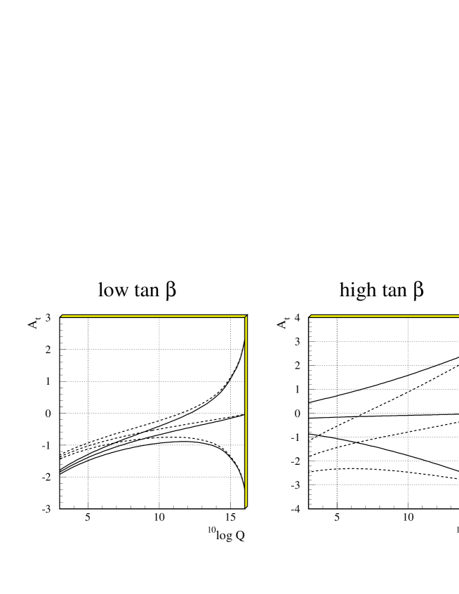
Figure 1: The running of $A_{t}$. The values of (${m_{0}},{m_{1/2}}$) were chosen to be (200,270) and (800,90) GeV for the low and high ${\tan\beta}$ scenario, respectively (solid lines) and (1000,1000) (dashed lines). At low values of ${\tan\beta}$ a strong convergence to a single value is found for all values of $A^{0}$ at the GUT scale, while for high values this tendency is less pronounced. The solid lines correspond to the preferred solutions of ref. [8].

CP-even Higgs Masses $m_{h,H}$.

The masses of the CP-even neutral higgses $H$ and $h$ are determined by the mass matrix

$${\cal M}=\frac{1}{2}\left(\frac{\partial^{2}V}{\partial\psi_{i}\partial\psi_{j}}\right)_{v_{1},v_{2}} = \left(\begin{array}[]{cc}\tan\beta&-1\\ -1&\cot\beta\end{array}\right)m_{3}^{2}+\frac{1}{2}\left(\begin{array}[]{cc}\cot\beta&-1\\ -1&\tan\beta\end{array}\right)M_{Z}^{2}\sin 2\beta$$ (17)

$$+ \frac{1}{2}\left(\begin{array}[]{cc}\Delta_{11}&\Delta_{12}\\ \Delta_{12}&\Delta_{22}\end{array}\right)$$ (20)

where $\psi_{i}$ are the real components of $H^{0}_{i}$ and

$$\Delta_{11} = \frac{1}{32\pi^{2}}\sum_{k}(-1)^{2J_{k}}(2J_{k}+1)c_{k}\left[\left(\frac{\partial m_{k}^{2}}{\partial\psi_{1}}\right)^{2}\log\frac{m_{k}^{2}}{Q^{2}}+\left(\frac{\partial^{2}m_{k}^{2}}{\partial\psi_{1}^{2}}-\frac{1}{\psi_{1}}\frac{\partial m_{k}^{2}}{\partial\psi_{1}}\right)f(m_{k}^{2})\right]$$

$$\Delta_{22} = \frac{1}{32\pi^{2}}\sum_{k}(-1)^{2J_{k}}(2J_{k}+1)c_{k}\left[\left(\frac{\partial m_{k}^{2}}{\partial\psi_{2}}\right)^{2}\log\frac{m_{k}^{2}}{Q^{2}}+\left(\frac{\partial^{2}m_{k}^{2}}{\partial\psi_{2}^{2}}-\frac{1}{\psi_{2}}\frac{\partial m_{k}^{2}}{\partial\psi_{2}}\right)f(m_{k}^{2})\right]$$

$$\Delta_{12} = \frac{1}{32\pi^{2}}\sum_{k}(-1)^{2J_{k}}(2J_{k}+1)c_{k}\left[\frac{\partial m_{k}^{2}}{\partial\psi_{1}}\frac{\partial m_{k}^{2}}{\partial\psi_{2}}\log\frac{m_{k}^{2}}{Q^{2}}+\frac{\partial^{2}m_{k}^{2}}{\partial\psi_{1}\partial\psi_{2}}f(m_{k}^{2})\right].$$ (21)

Diagonalization of the mass matrix yields after substituting the minimization conditions (2) and (3):

$$m^{2}_{h,H} = \frac{1}{2}\left[\frac{2m_{3}^{2}}{\sin 2\beta}+M^{2}_{Z}+\Delta_{11}+\Delta_{22}\mp\sqrt{\Delta^{2}_{h,H}}\right]$$ (22)

$$\Delta^{2}_{h,H} = (\frac{2m_{3}^{2}}{\sin 2\beta}+M_{Z}^{2}+\Delta_{11}+\Delta_{22})^{2}$$ (23)

$$- 4\frac{2m_{3}^{2}}{\sin 2\beta}M_{Z}^{2}\cos^{2}2\beta-4(\Delta_{11}\Delta_{22}-\Delta_{12}^{2})$$

$$- 4(\cos^{2}\beta M^{2}_{Z}+\sin^{2}\beta\frac{2m_{3}^{2}}{\sin 2\beta})\Delta_{22}$$

$$- 4(\sin^{2}\beta M^{2}_{Z}+\cos^{2}\beta\frac{2m_{3}^{2}}{\sin 2\beta})\Delta_{11}$$

$$- 4\sin 2\beta(M^{2}_{Z}+\frac{2m_{3}^{2}}{\sin 2\beta})\Delta_{12}.$$

The expressions for $\Delta_{ij}$ have been evaluated in Appendix C.

If $m_{A}\gg M_{Z}$ and if one considers only the contributions from the (s)top sector the formula for the lightest Higgs can be approximated as [12]:

$$m^{2}_{h} = M_{Z}^{2}\cos^{2}2\beta\left(1-\frac{3}{8\pi^{2}}\frac{m_{t}^{2}}{v^{2}}t\right)$$

$$+ \frac{3}{4\pi^{2}}\frac{m_{t}^{4}}{v^{2}}\left[\frac{1}{2}\tilde{X}_{t}+t+\frac{1}{16\pi^{2}}\left(\frac{3}{2}\frac{m_{t}^{2}}{v^{2}}-32\pi\alpha_{s}(M_{t})\right)(\tilde{X}_{t}+t^{2})\right]$$

where $\tilde{X}_{t}=2\tilde{A}_{t}^{2}/M^{2}_{SUSY}(1-\tilde{A}_{t}^{2}/12M^{2}_{SUSY})$, $\tilde{A}_{t}=A_{t}{m_{0}}-\mu\cot\beta,$ $t=\log(M^{2}_{SUSY}/M_{t}^{2})$, $m_{t}=m_{t}(M_{t})$ and $v=174$ GeV. $M_{SUSY}$ is a typical scale of the squark masses, which can be defined as the arithmetic average of the stop squared mass eigenvalues for not too large stop mass splittings. The last terms in eq. (3) proportional to $m_{t}^{6}$ and the strong coupling constant $\alpha_{s}$ take into account the most relevant two-loop corrections, which are absent in eq. (23).

It is important to note that the value of the trilinear coupling $A_{t}$ at the electroweak scale is not a free parameter, at least for low values of ${\tan\beta}$. In that case $A_{t}(M_{Z})$ goes to a fixed point solution, i.e. its value becomes independent of the starting value $A^{0}$ at the GUT scale. This is demonstrated in fig. 1 for several values of $m_{0}$ and $m_{1/2}$ and can be easily understood for the solution of the RGE’s in case $Y_{b}\ll Y_{t}$:

$$A_{t}(M_{Z})=A^{0}\left(1-\frac{Y_{t}}{Y_{f}}\right)-\frac{m_{1/2}}{m_{0}}\left(3.6-2.1\frac{Y_{t}}{Y_{f}}\right)\approx 0.009A^{0}-1.7\frac{m_{1/2}}{m_{0}},$$ (25)

where $Y_{f}$ is the fixed point solution of the Yukawa RGE and the numerical coefficients are taken from ref. [7]. For $m_{1/2}>m_{0}/6$ the last term is dominating, as long as $|A^{0}|<3$ (in units of $m_{0}$), which is the typical range for which tachyonic solutions and colour breaking minima in the scalar potential are avoided. For large values of ${\tan\beta}$ there is no simple analytical solution for $A_{t}$, since the bottom- and tau-Yukawa couplings cannot be neglected and the fixed point behaviour is less pronounced.

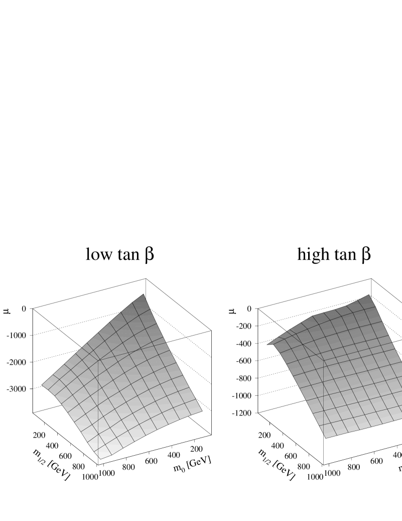
Figure 2: The value of the Higgs mixing parameter $\mu$ from EWSB as function of ${m_{0}}$ and ${m_{1/2}}$ for the low and high ${\tan\beta}$ scenario.

The Higgs mixing parameter $\mu$ can be determined from radiative electroweak symmetry breaking. Substituting

$$m^{2}_{H_{1}} = m_{1}^{2}-\mu^{2}$$ (26)

$$m^{2}_{H_{2}} = m_{2}^{2}-\mu^{2}$$

into eq. (2) yields:

$$\mu^{2} = \frac{m^{2}_{H_{1}}-m^{2}_{H_{2}}\tan^{2}\beta}{\tan^{2}\beta-1}+\frac{\Sigma_{1}-\Sigma_{2}\tan^{2}\beta}{\tan^{2}\beta-1}-\frac{M_{Z}^{2}}{2}\;\;.$$ (27)

The dependence of $\mu$ on $m_{0}$ and $m_{1/2}$ is shown in fig. 2. Due to the strong ${\tan\beta}$ dependence in eq. (27), the values are much smaller for the high ${\tan\beta}$ scenario. One observes that EWSB determines only $\mu^{2}$, so the mixing parameter $\tilde{A_{t}}$ in the stop sector can be either large or small, depending on the relative sign of $\mu$ and $A_{t}$. Both cases will be discussed.

Note that the mass of the CP-odd Higgs boson increases with $\mu^{2}$ (see eqs. (11) and (26)), so the Higgs mass $m_{A}$ is in practice always much larger than $M_{Z}$, if one determines $\mu$ from EWSB, at least for the low $\tan\beta$ scenario. For large values of $\tan\beta$ $\mu$ can become small, as can be seen from eq. (27), in which case $m_{A}$ is not necessary small compared with $M_{Z}$. Then $m_{h}$ becomes dependent on $m_{A}$ and the approximate formula from eq. (3) breaks down.

Note that the analytical formulae presented here are obtained using the effective potential approach (EPA), which samples the Green function at zero momentum and ignores the contribution to the wave function renormalization (WFR). The difference between our method and the explicit diagrammatic calculations (FDC )  [10, 11] is at most a few GeV as can be seen from the comparison in tab. 1.

		Mixing	$m_{h}^{max}$ in GeV
${m_{0}}$ in GeV	${m_{1/2}}$ in GeV	$A_{t,b,\tau}$	EPA	FDC
1000	2000	0	123.5	125.8
200	2000	0	94.2	96.9
1000	400	0	126.0	127.6
1000	2000	1	132.1	134.0

Table 1: Comparision of EPA Higgs limits with FDC calculations [10, 11] for different spectra: all susy particles heavy, light squarks/sleptons, light charginos/neutralinos, and large mixing in 3. generation sparticles. The mass of the pseudo scalar higgs boson $m_{A}$ in the above examples is $m_{A}=500$ GeV and the top mass $m_{t}=180$ GeV. For smaller top masses the differences are smaller.

4 Numerical Results

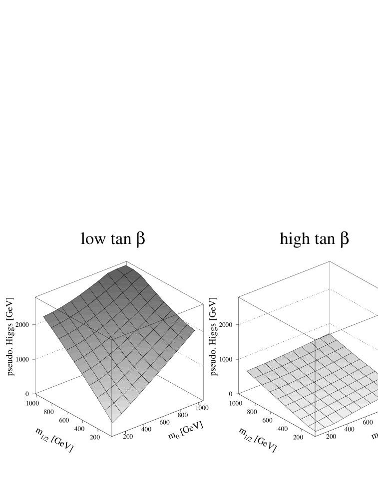
Figure 3: The mass of the CP-odd Higgs as function of ${m_{0}}$ and ${m_{1/2}}$ for the low and high ${\tan\beta}$ scenario, respectively. The lower values for high ${\tan\beta}$ originate from the lower values of $\mu$ required for EWSB in that case [8].

With the Higgs parameters $\mu$ and $\tan\beta$ determined from EWSB and bottom-tau unification, one can calculate all sparticle and Higgs masses as function of $m_{0}$ and $m_{1/2}$ including the corrections from all (s)particles in the loops. Since the CP-odd Higgs mass $m_{A}$ is for the most part of the parameter space much larger than $M_{Z}$ (see fig. 3), the mass of the lightest Higgs is mainly a function of the top mass only, since the $m_{A}$ dependence drops out, as discussed above. The top dependence is shown in fig. 4 for various cases. The upper scale indicates the value of $\tan\beta$ corresponding to the top mass for the low $\tan\beta$ scenario. In this case the Yukawa couplings $Y_{b}$ and $Y_{\tau}$ can be neglected and $\tan\beta$ can be directly calculated from the fixed point solution for $Y_{t}$, which yields approximately $m_{t}\approx 205\sin\beta$.

Figure 4: The mass of the lightest CP-even Higgs as function of the top mass at Born level (dotted lines), including complete one-loop contributions of all particles (dashed lines, $\mu>0$) for two values of the SUSY masses ${m_{0}}$ and ${m_{1/2}}$. Two-loop contributions reduce the one-loop corrections significantly as shown by the shaded area (the upper boundary corresponds to $\mu>0$, the lower one to $\mu<0$). The solid line just below the dashed line is the one-loop prediction from the third generation only, which apparently gives the main contribution.

Higgs masses in [GeV]
	Low ${\tan\beta}$							High ${\tan\beta}$
		$\mu<0$			$\mu>0$			$\mu<0$
Symbol	Born	$t,b,\tau$	All	+HO	$t,b,\tau$	All	+HO	Born	$t,b,\tau$	All	+HO
$m_{h}$	48	83	82	74	98	96	85	–	110	110	107
$m_{H}$	649	714	704	715	706	708	719	91	250	230	250
$m_{A}$	644	708	710	707	702	715	713	–	250	230	250
$m_{h}^{max~{}180}$	49	97	95	82	109	107	91	–	136	–	117
$m_{h}^{max~{}190}$	67	114	113	99	122	120	105	–	145	–	122

Table 2: Masses of the Higgs particles for the small and large $\tan\beta$ scenarios. The column with $t,b,\tau$ has only contribution from the third generation of particles, $All$ includes all particles in the loop and $+HO$ includes second order corrections from the renormalization group resummation, as given in ref. [12]. The numbers in the first three rows correspond to the following best fit parameters (in GeV) $m_{0}=200,m_{1/2}=270,\mu=\mp 1100,\mu(M_{Z})=\mp 525,{\tan\beta}=1.7$ and $m_{0}=800,m_{1/2}=90,\mu=-350,\mu(M_{Z})=-220,{\tan\beta}=41$, for the low and high ${\tan\beta}$ scenario, respectively. The last rows show the upper limit of the lightest Higgs mass corresponding to large SUSY masses ($m_{0}=m_{1/2}$=500 GeV) for $m_{t}=180$ and 190 GeV, respectively. The dashes for high $\tan\beta$ indicate non-physical negative Higgs masses.

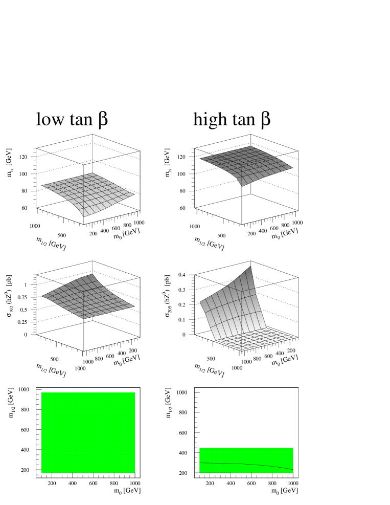
Figure 5: The mass of the lightest CP-even Higgs as function of ${m_{0}}$ and ${m_{1/2}}$ for the low and high ${\tan\beta}$ scenario on the left and right hand side. The top mass was taken to be 179 GeV and the sign of $\mu$ is negative, as required for the high ${\tan\beta}$ solution, but chosen negative for low ${\tan\beta}$. For high $\tan\beta$ the cross section is practically zero at the foreseen LEP II energy of 192 GeV, so only the cross section at the theoretically possible LEP II energy of 205 GeV is shown. The kinematical reach of the parameter space is shown by the contours of the third row: the whole parameter space can be covered for the low $\tan\beta$ scenario, while for high $\tan\beta$ the kinematic reach is about $m_{1/2}<450$ GeV and the solid line is the contour for $\sigma=0.2$ pb, which is roughly the exclusion limit[3].

Figure 6: The cross section as function of the center of mass energy for different Higgs masses, as indicated by the numbers (in GeV).

One observes the large one-loop corrections (upper lines) compared to the Born term (lowest lines) and the two-loop corrections[12] in-between. The dependence on the sign of $\mu$, which mainly influences the mixing parameter $\tilde{A}_{t}$, as discussed above, is shown by the grey area. Positive values of $\mu$ are not allowed for the large $\tan\beta$ scenario, because the large positive corrections to the bottom mass prohibit bottom-tau unification in that case. These corrections are small for small values of $\tan\beta$, so in that case one can choose either sign of $\mu$ (EWSB determines only $\mu^{2}$). Positive values of $\mu$ increase $m_{h}$ by 6 to 14 GeV, so the sign is quite important. Note that $\mu$ from EWSB is large (see fig. 2), so chaning the sign corresponds to large changes in the mixing.

The dominant contributions originate from the Yukawa couplings of the third generation, as demonstrated by the dashed lines in fig. 4: the Higgs masses including the third generation particles in the loops differ less than 3 GeV from the masses including the full corrections. For the large $\tan\beta$ scenario the largest contribution originates from the sbottom sector, as shown in Appendix D, where the individual contributions from all particles have been summarized. The masses of all SUSY particles as obtained from the RG equations in ref. [8] are given too.

Note the large single contributions to $\Sigma_{1}$ and $\Sigma_{2}$. However, if the masses of the left and right handed partners are equal, they cancel in the sum of $\Sigma_{1}$ and $\Sigma_{2}$. The contributions from Higgses, charginos, neutralinos and sparticles of the third generation with a large mixing between left and right handed partners does not cancel and one obtains large one-loop corrections.

For the lightest Higgs the large contributions from $\Sigma_{1}$ and $\Sigma_{2}$ are partially cancelled against the corrections in $\Delta_{ij}$, since they contain similar terms with opposite signs ($\frac{1}{\Psi_{1/2}}\frac{\partial m_{k}^{2}}{\partial\Psi_{1/2}}$ in eqs. (4), (5) and (21)). In the formula for the Higgs mass, eq. (22), these corrections are summed. Nevertheless, at large ${\tan\beta}$ the resulting corrections are still large, as can be seen by adding the bottom lines of tables 3, 4 and 5. Note that the $\Sigma_{1(2)}$ contributions of table 3 must be weighted by $\frac{1}{\sin 2\beta}\approx 0.05$, as one can see in eqs. (3) and (23).

The curves on the left side in fig. 4 are shown for $m_{0}=200,m_{1/2}=270$, which is the solution yielding the best fit to the low energy constraints [8]. On the right hand side $m_{0}$ and ${m_{1/2}}$ are set to 500 GeV, which corresponds to squarks masses around 1 TeV. In this case one obtains upper limits on $m_{h}$, since the Higgs mass saturates for such large values, as shown in fig. 5. Here the one-loop Higgs mass is plotted as function of ${m_{0}}$ and ${m_{1/2}}$ for $\mu<0$. For $\mu>0$ the Higgs mass increases, but the second order corrections decrease it again by roughly the same amount, as summarized numerically in table 2 for various conditions, so fig. 5 is a good representation for the most pessimistic case of $\mu>0$ too, if the second order corrections are included.

For large $\tan\beta$ the Higgs masses are outside the reach of LEP II with a maximum energy of 192 GeV. But for the low $\tan\beta$ scenario the Higgs cross section is large enough for the whole parameter space of $m_{0}$ and $m_{1/2}$, as shown in fig. 5, at least if the top mass is around 180 GeV.

The small region of parameter space covered by LEP II at 205 GeV in case of the high ${\tan\beta}$ scenario is shown by the solid line in the bottom part of fig. 5. It is assumed, that a luminosity of 0.2 pb is needed for the Higgs search, as estimated by the LEP II working group [3]. At a LEP II energy of 192 GeV the high ${\tan\beta}$ scenario of the CMSSM is out of reach. Also the channel $e^{+}e^{-}\to hA$ is not accessible at LEP II for most of the parameter space because of the large values of $m_{A}$ predicted in the CMSSM (basically because of the large value of $\mu$ required by EWSB). The center of mass energy dependence of the Higgs-strahlungs cross section is summarized in fig. 6 for various Higgs masses.

5 Summary

Within the framework of the Minimal Supersymmetric Standard Model (MSSM) the Higgs masses and LEP II production cross sections have been calculated including the D-terms and complete one-loop contributions of all sparticles, for which explicit analytical formulae are derived. As expected, the radiative corrections from the Yukawa couplings of the third generation dominate over the contributions from charginos and neutralinos. This implies that the simple analytical formula of eq. 3 is a good approximation. In this case the maximal Higgs mass is reached for ”maximal” mixing, i.e. maximal $\tilde{X}_{t}$, which occurs for $\tilde{A}_{t}=\sqrt{6}M_{SUSY}$. In the CMSSM maximal mixing does not occur, since $\tilde{A}_{t}\approx M_{SUSY}$, if $A_{t}$ is determined from the fixed point solution for $A_{t}$ (eq. 25) and $\mu$ from EWSB (eq. 27).

For the low ${\tan\beta}$ scenario the mass of the lightest Higgs is found to be below 90 GeV for a top mass below 180 GeV. The cross section at a LEP II energy of 192 GeV is sufficient to find or exclude this low ${\tan\beta}$ scenario. For the high ${\tan\beta}$ scenario only a small fraction of the parameter space can be covered, since the Higgs mass is predicted between 105 and 122 GeV in most cases. It should be noted that the predicted upper limit of the Higgs mass is somewhat lower (up to 10 GeV) than the one given by the LEP Working Group [3], because they assume maximal mixing, which does not occur in the CMSSM.

Note added in proof:
After finishing our results a new publication containing all one-loop corrections to all masses and couplings of the MSSM appeared[15].¸ Concerning the Higgs boson masses our results (within the EPA approach) are more explicit and contain individual contributions coming from different particles together with their numerical values for low and high ${\tan\beta}$.

Acknowledgment

This work was supported from the Bundesministerium für Bildung, Wissenschaft, Forschung und Technologie (BMBF Contract CERN-LEP-DELPHI 05 6KA16P 3), the Deutsche Forschungsgemeinschaft (DFG) for our ”Graduiertenkolleg” and the European Community (HCM Network Contract ERBCHRXCT930345) and Russian Foundation for Basic Research (Grant RFBR-96-02-17379).

Appendix A

In this appendix we summarize the tree-level field-dependent masses of all particles contributing to the one-loop corrections to the effective Higgs potential.

Quark and Lepton Masses.

$$m_{q}^{2} = h_{q}^{2}|H_{i}^{0}|^{2},\;\;\;\;\;{\rm where}\left\{\begin{array}[]{ll}i=2&{\rm for}\;\;up\;\;quarks\\ i=1&{\rm for}\;\;down\;\;quarks\end{array}\right.$$

$$m_{l}^{2} = h_{l}^{2}|H_{1}^{0}|^{2}$$

Gauge Boson Masses.

$$M^{2}_{W^{\pm}} = \frac{g^{2}}{2}(|H_{1}^{0}|^{2}+|H_{2}^{0}|^{2})$$

$$M^{2}_{Z^{0}} = \frac{g^{2}+g^{\prime 2}}{2}(|H_{1}^{0}|^{2}+|H_{2}^{0}|^{2})$$

Higgs Boson Masses.

$$m_{A}^{2} = m_{1}^{2}+m_{2}^{2}$$

$$m^{2}_{H^{\pm}} = m_{A}^{2}+M_{W}^{2}$$

$$m^{2}_{H,h} = \frac{1}{2}\left[m_{A}^{2}+M_{Z}^{2}\pm\sqrt{(m_{A}^{2}+M_{Z}^{2})^{2}-4m_{A}^{2}M_{Z}^{2}\cos^{2}2\beta}\right]$$

Chargino and Neutralino Masses.

The chargino mass matrix is:

$$M^{(c)}=\left(\begin{array}[]{cc}M_{2}&g|H_{2}^{0}|\\ g|H_{1}^{0}|&\mu\end{array}\right)$$ (29)

where $M_{2}$ is the mass of the $SU(2)_{L}$ gaugino, the Wino.

After diagonalization one obtains:

$$\tilde{m}^{2}_{\chi_{1,2}^{\pm}} = \frac{1}{2}\left[M_{2}^{2}+\mu^{2}+2M_{W}^{2}\right.$$

$$\left.\pm\sqrt{(M_{2}^{2}-\mu^{2})^{2}+4M_{W}^{4}\cos^{2}2\beta+4M_{W}^{2}(M_{2}^{2}+\mu^{2}+2M_{2}\mu\sin 2\beta)}\right]$$

The neutralino mass matrix is:

$$M^{(0)}=\left(\begin{array}[]{cccc}M_{1}&0&-\frac{g^{\prime}}{\sqrt{2}}|H_{1}^{0}|&\frac{g^{\prime}}{\sqrt{2}}|H_{2}^{0}|\\ 0&M_{2}&\frac{g}{\sqrt{2}}|H_{1}^{0}|&-\frac{g}{\sqrt{2}}|H_{2}^{0}|\\ -\frac{g^{\prime}}{\sqrt{2}}|H_{1}^{0}|&\frac{g}{\sqrt{2}}|H_{1}^{0}|&0&-\mu\\ \frac{g^{\prime}}{\sqrt{2}}|H_{2}^{0}|&-\frac{g}{\sqrt{2}}|H_{2}^{0}|&-\mu&0\end{array}\right)$$ (30)

Again $M_{2}$ is the mass of the Wino, whereas $M_{1}$ is the mass of the $U(1)_{Y}$ gaugino, the Bino. The neutralino masses $\tilde{m}_{\chi^{0}}$ are the roots $\lambda_{k}$ of quartic equation $F(\lambda)=0$, where

$$F(\lambda) = \lambda^{4}-(M_{1}+M_{2})\lambda^{3}-(M_{Z}^{2}+\mu^{2}-M_{1}M_{2})\lambda^{2}$$ (31)

$$+[(M_{2}\sin^{2}\theta_{W}+M_{1}\cos^{2}\theta_{W}-\mu\sin 2\beta)M_{Z}^{2}+(M_{1}+M_{2})\mu^{2}]\lambda$$

$$+[(M_{2}\sin^{2}\theta_{W}+M_{1}\cos^{2}\theta_{W})\mu M_{Z}^{2}\sin 2\beta-M_{1}M_{2}\mu^{2}]$$

Squark and Slepton Masses.

The top and the bottom squark and tau-slepton mass-squared matrices:

$${\cal M}^{\tilde{t}}=\left(\begin{array}[]{cc}\tilde{m}_{t_{L}}^{2}&m_{t}(A_{t}m_{0}-\mu\cot\beta)\\ m_{t}(A_{t}m_{0}-\mu\cot\beta)&\tilde{m}_{t_{R}}^{2}\end{array}\right),$$ (32)

$${\cal M}^{\tilde{b}}=\left(\begin{array}[]{cc}\tilde{m}_{b_{L}}^{2}&m_{b}(A_{b}m_{0}-\mu\tan\beta)\\ m_{b}(A_{b}m_{0}-\mu\tan\beta)&\tilde{m}_{b_{R}}^{2}\end{array}\right),$$ (33)

$${\cal M}^{\tilde{\tau}}=\left(\begin{array}[]{cc}\tilde{m}_{\tau_{L}}^{2}&m_{\tau}(A_{\tau}m_{0}-\mu\tan\beta)\\ m_{\tau}(A_{\tau}m_{0}-\mu\tan\beta)&\tilde{m}_{\tau_{R}}^{2}\end{array}\right).$$ (34)

The diagonalization of these matrices yields expressions for the masses of the third generation squarks and sleptons:

$$\tilde{m}_{t_{1,2}}^{2} = \frac{1}{2}\left(\tilde{m}_{t_{L}}^{2}+\tilde{m}_{t_{R}}^{2}\right)\mp\sqrt{\frac{1}{4}\left(\tilde{m}_{t_{L}}^{2}-\tilde{m}_{t_{R}}^{2}\right)^{2}+m_{t}^{2}(A_{t}m_{0}-\mu\cot\beta)^{2}},$$ (35)

$$\tilde{m}_{b_{1,2}}^{2} = \frac{1}{2}\left(\tilde{m}_{b_{L}}^{2}+\tilde{m}_{b_{R}}^{2}\right)\mp\sqrt{\frac{1}{4}\left(\tilde{m}_{b_{L}}^{2}-\tilde{m}_{b_{R}}^{2}\right)^{2}+m_{b}^{2}(A_{b}m_{0}-\mu\tan\beta)^{2}},$$ (36)

$$\tilde{m}_{\tau_{1,2}}^{2} = \frac{1}{2}\left(\tilde{m}_{\tau_{L}}^{2}+\tilde{m}_{\tau_{R}}^{2}\right)\mp\sqrt{\frac{1}{4}\left(\tilde{m}_{\tau_{L}}^{2}-\tilde{m}_{\tau_{R}}^{2}\right)^{2}+m_{\tau}^{2}(A_{\tau}m_{0}-\mu\tan\beta)^{2}}.$$ (37)

The mass eigenstate for the massive third generation sneutrino is:

$$\tilde{m}_{\nu_{\tau}}^{2}=M_{L}^{2}+\frac{1}{2}M_{Z}^{2}\cos 2\beta$$ (38)

where $M_{L}$ is the breaking mass of the 3. generation Sleptons of the $SU(2)_{L}$ doublet.

Appendix B

We present here analytical formulae for the contributions from all particles to $\Sigma_{1}$ and $\Sigma_{2}$ from eqs. (4) and (5). Some of these formulae can be also found in ref. [6]. In most cases they coincide with ours, however we have found obvious misprints.

$$\Sigma_{1}^{W^{\pm}} = \frac{3g^{2}}{32\pi^{2}}f(M^{2}_{W^{\pm}})$$

$$\Sigma_{2}^{W^{\pm}} = \frac{3g^{2}}{32\pi^{2}}f(M^{2}_{W^{\pm}})$$

$$\Sigma_{1}^{Z^{0}} = \frac{3g^{2}}{64\pi^{2}\cos^{2}\theta_{W}}f(M^{2}_{Z})$$

$$\Sigma_{2}^{Z^{0}} = \frac{3g^{2}}{64\pi^{2}\cos^{2}\theta_{W}}f(M^{2}_{Z})$$

$$\Sigma_{1}^{H^{\pm}} = \frac{g^{2}}{32\pi^{2}}f(m^{2}_{H^{\pm}})$$

$$\Sigma_{2}^{H^{\pm}} = \frac{g^{2}}{32\pi^{2}}f(m^{2}_{H^{\pm}})$$

$$\Sigma_{1}^{H,h} = \frac{g^{2}}{128\pi^{2}\cos^{2}\theta_{W}}\left[1\pm\frac{M_{Z}^{2}+m_{A}^{2}(1-4\cos 2\beta+2\cos^{2}2\beta)}{m_{H}^{2}-m_{h}^{2}}\right]f(m^{2}_{H,h})$$

$$\Sigma_{2}^{H,h} = \frac{g^{2}}{128\pi^{2}\cos^{2}\theta_{W}}\left[1\pm\frac{M_{Z}^{2}+m_{A}^{2}(1+4\cos 2\beta+2\cos^{2}2\beta)}{m_{H}^{2}-m_{h}^{2}}\right]f(m^{2}_{H,h})$$

$$\Sigma_{1}^{\tilde{\chi}_{1,2}^{\pm}} = -\frac{g^{2}}{16\pi^{2}}\left[1\pm\frac{2M_{W}^{2}\cos 2\beta+M_{2}^{2}+\mu^{2}+2M_{2}\mu\tan\beta}{\tilde{m}^{2}_{\chi_{1}^{\pm}}-\tilde{m}^{2}_{\chi_{2}^{\pm}}}\right]f(\tilde{m}^{2}_{\chi_{1,2}^{\pm}})$$

$$\Sigma_{2}^{\tilde{\chi}_{1,2}^{\pm}} = -\frac{g^{2}}{16\pi^{2}}\left[1\pm\frac{-2M_{W}^{2}\cos 2\beta+M_{2}^{2}+\mu^{2}+2M_{2}\mu\cot\beta}{\tilde{m}^{2}_{\chi_{1}^{\pm}}-\tilde{m}^{2}_{\chi_{2}^{\pm}}}\right]f(\tilde{m}^{2}_{\chi_{1,2}^{\pm}})$$

$$\Sigma_{1}^{\tilde{\chi}^{0}} = -\frac{g^{2}}{16\pi^{2}}\frac{M_{Z}^{2}}{M_{W}^{2}}\sum\limits_{k=1}^{4}\frac{\lambda_{k}(\lambda_{k}-\tilde{m}_{\gamma})(\lambda_{k}+\mu\tan\beta)}{D(\lambda_{k})}f(\lambda_{k}^{2})$$

$$\Sigma_{2}^{\tilde{\chi}^{0}} = -\frac{g^{2}}{16\pi^{2}}\frac{M_{Z}^{2}}{M_{W}^{2}}\sum\limits_{k=1}^{4}\frac{\lambda_{k}(\lambda_{k}-\tilde{m}_{\gamma})(\lambda_{k}+\mu\cot\beta)}{D(\lambda_{k})}f(\lambda_{k}^{2})$$

$$\Sigma_{1}^{t} = 0$$

$$\Sigma_{2}^{t} = -\frac{3g^{2}}{16\pi\cos^{2}\theta_{W}}\frac{m_{t}^{2}}{M_{Z}^{2}\sin^{2}\beta}f(m_{t}^{2})$$

$$\Sigma_{1}^{\tilde{t}_{1,2}} = \frac{3g^{2}}{32\pi^{2}\cos^{2}\theta_{W}}f(\tilde{m}^{2}_{t_{1,2}})\Biggl{\{}\frac{1}{4}\pm\frac{1}{\tilde{m}^{2}_{t_{1}}-\tilde{m}^{2}_{t_{2}}}$$

$$\times\biggl{[}\frac{-m^{2}_{t}\mu}{M^{2}_{Z}\sin^{2}\beta}\left(A_{t}m_{0}\tan\beta-\mu\right)+\frac{1}{2}\left(\frac{1}{2}-\frac{4}{3}\sin^{2}\theta_{W}\right)\left(\tilde{m}^{2}_{t_{L}}-\tilde{m}^{2}_{t_{R}}\right)\biggr{]}\Biggr{\}}$$

$$\Sigma_{2}^{\tilde{t}_{1,2}} = \frac{3g^{2}}{32\pi^{2}\cos^{2}\theta_{W}}f(\tilde{m}^{2}_{t_{1,2}})\Biggl{\{}\frac{m^{2}_{t}}{M^{2}_{Z}\sin^{2}\beta}-\frac{1}{4}\pm\frac{1}{\tilde{m}^{2}_{t_{1}}-\tilde{m}^{2}_{t_{2}}}$$

$$\times\biggl{[}\frac{m^{2}_{t}A_{t}m_{0}}{M^{2}_{Z}\sin^{2}\beta}\left(A_{t}m_{0}-\mu\cot\beta\right)-\frac{1}{2}\left(\frac{1}{2}-\frac{4}{3}\sin^{2}\theta_{W}\right)\left(\tilde{m}^{2}_{t_{L}}-\tilde{m}^{2}_{t_{R}}\right)\biggr{]}\Biggr{\}}$$

$$\Sigma_{1}^{b} = -\frac{3g^{2}}{16\pi\cos^{2}\theta_{W}}\frac{m_{b}^{2}}{M_{Z}^{2}\cos^{2}\beta}f(m_{b}^{2})$$

$$\Sigma_{2}^{b} = 0$$

$$\Sigma_{1}^{\tilde{b}_{1,2}} = \frac{3g^{2}}{32\pi^{2}\cos^{2}\theta_{W}}f(\tilde{m}^{2}_{b_{1,2}})\Biggl{\{}\frac{m^{2}_{b}}{M^{2}_{Z}\cos^{2}\beta}-\frac{1}{4}\pm\frac{1}{\tilde{m}^{2}_{b_{1}}-\tilde{m}^{2}_{b_{2}}}$$

$$\times\biggl{[}\frac{m^{2}_{b}A_{b}m_{0}}{M^{2}_{Z}\cos^{2}\beta}\left(A_{b}m_{0}-\mu\tan\beta\right)-\frac{1}{2}\left(\frac{1}{2}-\frac{2}{3}\sin^{2}\theta_{W}\right)\left(\tilde{m}^{2}_{b_{L}}-\tilde{m}^{2}_{b_{R}}\right)\biggr{]}\Biggr{\}}$$

$$\Sigma_{2}^{\tilde{b}_{1,2}} = \frac{3g^{2}}{32\pi^{2}\cos^{2}\theta_{W}}f(\tilde{m}^{2}_{b_{1,2}})\Biggl{\{}\frac{1}{4}\pm\frac{1}{\tilde{m}^{2}_{b_{1}}-\tilde{m}^{2}_{b_{2}}}$$

$$\times\biggl{[}\frac{-m^{2}_{b}\mu}{M^{2}_{Z}\cos^{2}\beta}\left(A_{b}m_{0}\cot\beta-\mu\right)+\frac{1}{2}\left(\frac{1}{2}-\frac{2}{3}\sin^{2}\theta_{W}\right)\left(\tilde{m}^{2}_{b_{L}}-\tilde{m}^{2}_{b_{R}}\right)\biggr{]}\Biggr{\}}$$

$$\Sigma_{1}^{\tau} = -\frac{g^{2}}{16\pi\cos^{2}\theta_{W}}\frac{m_{\tau}^{2}}{M_{Z}^{2}\cos^{2}\beta}f(m_{\tau}^{2})$$

$$\Sigma_{2}^{\tau} = 0$$

$$\Sigma_{1}^{\tilde{\tau}_{1,2}} = \frac{3g^{2}}{32\pi^{2}\cos^{2}\theta_{W}}f(\tilde{m}^{2}_{\tau_{1,2}})\Biggl{\{}\frac{m^{2}_{\tau}}{M^{2}_{Z}\cos^{2}\beta}-\frac{1}{4}\pm\frac{1}{\tilde{m}^{2}_{\tau_{1}}-\tilde{m}^{2}_{\tau_{2}}}$$

$$\times\biggl{[}\frac{m^{2}_{\tau}A_{\tau}m_{0}}{M^{2}_{Z}\cos^{2}\beta}\left(A_{\tau}m_{0}-\mu\tan\beta\right)-\frac{1}{2}\left(\frac{1}{2}-2\sin^{2}\theta_{W}\right)\left(\tilde{m}^{2}_{\tau_{L}}-\tilde{m}^{2}_{\tau_{R}}\right)\biggr{]}\Biggr{\}}$$

$$\Sigma_{2}^{\tilde{\tau}_{1,2}} = \frac{3g^{2}}{32\pi^{2}\cos^{2}\theta_{W}}f(\tilde{m}^{2}_{\tau_{1,2}})\Biggl{\{}\frac{1}{4}\pm\frac{1}{\tilde{m}^{2}_{\tau_{1}}-\tilde{m}^{2}_{\tau_{2}}}$$

$$\times\biggl{[}\frac{-m^{2}_{\tau}\mu}{M^{2}_{Z}\cos^{2}\beta}\left(A_{\tau}m_{0}\cot\beta-\mu\right)+\frac{1}{2}\left(\frac{1}{2}-\frac{2}{3}\sin^{2}\theta_{W}\right)\left(\tilde{m}^{2}_{\tau_{L}}-\tilde{m}^{2}_{\tau_{R}}\right)\biggr{]}\Biggr{\}}$$

Appendix C

Here analytical formulae for the contributions from all particles to $\Delta_{11},\Delta_{22}$ and $\Delta_{12}$ in eq. (21) are presented. In the literature often $m_{A}$ is considered as a free parameter. In our framework this can be achieved, if the CP-even mass matrix eq. (20) is rewritten as:

$${\cal M}=\frac{1}{2}\left(\frac{\partial^{2}V}{\partial\psi_{i}\partial\psi_{j}}\right)_{v_{1},v_{2}} = \frac{1}{2}\left(\begin{array}[]{cc}\tan\beta&-1\\ -1&\cot\beta\end{array}\right)m_{A_{1-loop}}^{2}\sin 2\beta+\frac{1}{2}\left(\begin{array}[]{cc}\cot\beta&-1\\ -1&\tan\beta\end{array}\right)M_{Z}^{2}\sin 2\beta$$ (43)

$$+ \frac{1}{2}\left(\begin{array}[]{cc}\Delta_{11}-\tan\beta\;\Delta&\Delta_{12}+\Delta\\ \Delta_{12}+\Delta&\Delta_{22}-\cot\beta\;\Delta\end{array}\right)$$ (46)

where $\Delta$ are the corrections from eq. (3) and $\sin 2\beta\;m_{A_{1-loop}}^{2}=2m_{3}^{2}+\Delta$ (11). Thus taking $m_{A}$ as free input parameter, one has to subtract the terms proportional $\Delta$ in $\Delta_{11}$, $\Delta_{12}$, and $\Delta_{22}$, having in mind, that they are compensated with the corresponding corrections in $m_{A}$.

Contribution from $W^{\pm},Z^{0}$.

$$\Delta_{11} = \frac{3g^{2}}{16\pi^{2}}M_{Z}^{2}\left[(2\cos^{2}\theta_{W}+\cos^{-2}\theta_{W})\log\frac{M_{Z}^{2}}{Q^{2}}+2\cos^{2}\theta_{W}\log\cos^{2}\theta_{W}\right]\cos^{2}\beta$$

$$\Delta_{22} = \frac{3g^{2}}{16\pi^{2}}M_{Z}^{2}\left[(2\cos^{2}\theta_{W}+\cos^{-2}\theta_{W})\log\frac{M_{Z}^{2}}{Q^{2}}+2\cos^{2}\theta_{W}\log\cos^{2}\theta_{W}\right]\sin^{2}\beta$$

$$\Delta_{12} = \frac{3g^{2}}{16\pi^{2}}M_{Z}^{2}\left[(2\cos^{2}\theta_{W}+\cos^{-2}\theta_{W})\log\frac{M_{Z}^{2}}{Q^{2}}+2\cos^{2}\theta_{W}\log\cos^{2}\theta_{W}\right]\sin\beta\cos\beta$$

Contribution from $H^{\pm}$.

$$\Delta_{11} = \frac{g^{2}}{8\pi^{2}}M_{W}^{2}\log\frac{m_{A}^{2}+M_{W}^{2}}{Q^{2}}\cos^{2}\beta$$

$$\Delta_{22} = \frac{g^{2}}{8\pi^{2}}M_{W}^{2}\log\frac{m_{A}^{2}+M_{W}^{2}}{Q^{2}}\sin^{2}\beta$$

$$\Delta_{12} = \frac{g^{2}}{8\pi^{2}}M_{W}^{2}\log\frac{m_{A}^{2}+M_{W}^{2}}{Q^{2}}\sin\beta\cos\beta$$

Contribution from H,h.

$$\Delta_{11} = \frac{g^{2}}{64\pi^{2}}\frac{M_{Z}^{2}}{M_{W}^{2}}\left[M_{Z}^{2}\left(\log\frac{m_{H}^{2}m_{h}^{2}}{Q^{4}}+2\rho_{1}\log\frac{m_{H}^{2}}{m_{h}^{2}}+\rho_{1}^{2}d(m_{H}^{2},m_{h}^{2})\right)\right.$$

$$+\left.2(M_{Z}^{2}-16m_{A}^{2}\sin^{4}\beta)\frac{f(m_{H}^{2})-f(m_{h}^{2})}{m_{H}^{2}-m_{h}^{2}}\right]\cos^{2}\beta$$

$$\Delta_{22} = \frac{g^{2}}{64\pi^{2}}\frac{M_{Z}^{2}}{M_{W}^{2}}\left[M_{Z}^{2}\left(\log\frac{m_{H}^{2}m_{h}^{2}}{Q^{4}}+2\rho_{2}\log\frac{m_{H}^{2}}{m_{h}^{2}}+\rho_{2}^{2}d(m_{H}^{2},m_{h}^{2})\right)\right.$$

$$+\left.2(M_{Z}^{2}-16m_{A}^{2}\cos^{4}\beta)\frac{f(m_{H}^{2})-f(m_{h}^{2})}{m_{H}^{2}-m_{h}^{2}}\right]\sin^{2}\beta$$

$$\Delta_{12} = \frac{g^{2}}{64\pi^{2}}\frac{M_{Z}^{2}}{M_{W}^{2}}\left[M_{Z}^{2}\left(\log\frac{m_{H}^{2}m_{h}^{2}}{Q^{4}}+(\rho_{1}+\rho_{2})\log\frac{m_{H}^{2}}{m_{h}^{2}}+\rho_{1}\rho_{2}d(m_{H}^{2},m_{h}^{2})\right)\right.$$

$$+\left.2(M_{Z}^{2}+16m_{A}^{2}\sin^{2}\cos^{2}\beta)\frac{f(m_{H}^{2})-f(m_{h}^{2})}{m_{H}^{2}-m_{h}^{2}}\right]\sin\beta\cos\beta$$

where

$$\rho_{1} = \frac{M_{Z}^{2}+m_{A}^{2}(1-4\cos 2\beta+2\cos^{2}2\beta)}{m_{H}^{2}-m_{h}^{2}}$$

$$\rho_{2} = \frac{M_{Z}^{2}+m_{A}^{2}(1+4\cos 2\beta+2\cos^{2}2\beta)}{m_{H}^{2}-m_{h}^{2}}$$

$$d(m_{1}^{2},m_{2}^{2})=2-\frac{m_{1}^{2}+m_{2}^{2}}{m_{1}^{2}-m_{2}^{2}}\log\frac{m_{1}^{2}}{m_{2}^{2}}$$

Chargino contribution.

$$\Delta_{11} = -\frac{g^{2}}{4\pi^{2}}\left[M_{W}^{2}\left(\log\frac{m_{\chi_{1}^{\pm}}^{2}m_{\chi_{2}^{\pm}}^{2}}{Q^{4}}+2\eta_{1}\log\frac{m_{\chi_{1}^{\pm}}^{2}}{m_{\chi_{2}^{\pm}}^{2}}+\eta_{1}^{2}d(m_{\chi_{1}^{\pm}}^{2},m_{\chi_{2}^{\pm}}^{2})\right)\right.$$

$$+\left.\left(2M_{W}^{2}-M_{2}\mu\frac{\sin\beta}{\cos^{3}\beta}\right)\frac{f(m_{\chi_{1}^{\pm}}^{2})-f(m_{\chi_{2}^{\pm}}^{2})}{m_{\chi_{1}^{\pm}}^{2}-m_{\chi_{2}^{\pm}}^{2}}\right]\cos^{2}\beta$$

$$\Delta_{22} = -\frac{g^{2}}{4\pi^{2}}\left[M_{W}^{2}\left(\log\frac{m_{\chi_{1}^{\pm}}^{2}m_{\chi_{2}^{\pm}}^{2}}{Q^{4}}+2\eta_{2}\log\frac{m_{\chi_{1}^{\pm}}^{2}}{m_{\chi_{2}^{\pm}}^{2}}+\eta_{2}^{2}d(m_{\chi_{1}^{\pm}}^{2},m_{\chi_{2}^{\pm}}^{2})\right)\right.$$

$$+\left.\left(2M_{W}^{2}-M_{2}\mu\frac{\cos\beta}{\sin^{3}\beta}\right)\frac{f(m_{\chi_{1}^{\pm}}^{2})-f(m_{\chi_{2}^{\pm}}^{2})}{m_{\chi_{1}^{\pm}}^{2}-m_{\chi_{2}^{\pm}}^{2}}\right]\sin^{2}\beta$$

$$\Delta_{12} = -\frac{g^{2}}{4\pi^{2}}\left[M_{W}^{2}\left(\log\frac{m_{\chi_{1}^{\pm}}^{2}m_{\chi_{2}^{\pm}}^{2}}{Q^{4}}+(\eta_{1}+\eta_{2})\log\frac{m_{\chi_{1}^{\pm}}^{2}}{m_{\chi_{2}^{\pm}}^{2}}+\eta_{1}\eta_{2}d(m_{\chi_{1}^{\pm}}^{2},m_{\chi_{2}^{\pm}}^{2})\right)\right.$$

$$-\left.\left(2M_{W}^{2}-M_{2}\mu\frac{1}{\sin\beta\cos\beta}\right)\frac{f(m_{\chi_{1}^{\pm}}^{2})-f(m_{\chi_{2}^{\pm}}^{2})}{m_{\chi_{1}^{\pm}}^{2}-m_{\chi_{2}^{\pm}}^{2}}\right]\sin\beta\cos\beta$$

where

$$\eta_{1} = \frac{2M_{W}^{2}\cos 2\beta+M_{2}^{2}+\mu^{2}+2M_{2}\mu\tan\beta}{m_{\chi_{1}^{\pm}}^{2}-m_{\chi_{2}^{\pm}}^{2}}$$

$$\eta_{2} = \frac{-2M_{W}^{2}\cos 2\beta+M_{2}^{2}+\mu^{2}+2M_{2}\mu\cot\beta}{m_{\chi_{1}^{\pm}}^{2}-m_{\chi_{2}^{\pm}}^{2}}$$

Neutralino contribution.

$$\Delta_{11} = -\frac{g^{2}}{8\pi^{2}}\frac{M_{Z}^{2}}{M_{W}^{2}}\cos^{2}\beta\sum_{k=1}^{4}\left[2M_{Z}^{2}\left(2\lambda_{k}^{2}\frac{\tau_{1}^{2}(\lambda_{k})}{D^{2}(\lambda_{k})}\log\frac{\lambda_{k}^{2}}{Q^{2}}+\frac{\tau_{1}^{2}\left(1-\lambda_{k}\frac{D^{\prime}(\lambda_{k})}{D(\lambda_{k})}\right)}{D^{2}(\lambda_{k})}f(\lambda_{k}^{2})\right.\right.$$

$$\left.\left.+\frac{2\tau_{1}\lambda_{k}(2\lambda_{k}-\tilde{m}_{\gamma}+\mu\tan\beta)}{D^{2}(\lambda_{k})}f(\lambda_{k}^{2})\right)-\frac{\lambda_{k}\mu(\lambda_{k}-\tilde{m}_{\gamma})}{D(\lambda_{k})}\frac{\sin\beta}{\cos^{3}\beta}f(\lambda_{k}^{2})\right]$$

$$\Delta_{22} = -\frac{g^{2}}{8\pi^{2}}\frac{M_{Z}^{2}}{M_{W}^{2}}\sin^{2}\beta\sum_{k=1}^{4}\left[2M_{Z}^{2}\left(2\lambda_{k}^{2}\frac{\tau_{2}^{2}(\lambda_{k})}{D^{2}(\lambda_{k})}\log\frac{\lambda_{k}^{2}}{Q^{2}}+\frac{\tau_{2}^{2}\left(1-\lambda_{k}\frac{D^{\prime}(\lambda_{k})}{D(\lambda_{k})}\right)}{D^{2}(\lambda_{k})}f(\lambda_{k}^{2})\right.\right.$$

$$\left.\left.+\frac{2\tau_{2}\lambda_{k}(2\lambda_{k}-\tilde{m}_{\gamma}-\mu\cot\beta)}{D^{2}(\lambda_{k})}f(\lambda_{k}^{2})\right)-\frac{\lambda_{k}\mu(\lambda_{k}-\tilde{m}_{\gamma})}{D(\lambda_{k})}\frac{\cos\beta}{\sin^{3}\beta}f(\lambda_{k}^{2})\right]$$

$$\Delta_{12} = -\frac{g^{2}}{8\pi^{2}}\frac{M_{Z}^{2}}{M_{W}^{2}}\sin\beta\cos\beta\sum_{k=1}^{4}\left[2M_{Z}^{2}\left(2\lambda_{k}^{2}\frac{\tau_{1}\tau_{2}}{D^{2}}\log\frac{\lambda_{k}^{2}}{Q^{2}}+\frac{\tau_{1}\tau_{2}\left(1-\lambda_{k}\frac{D^{\prime}}{D}\right)}{D^{2}(\lambda_{k})}f(\lambda_{k}^{2})\right.\right.$$

$$\left.+\frac{\lambda_{k}[\tau_{1}(2\lambda_{k}-\tilde{m}_{\gamma}+\mu\cot\beta)+\tau_{2}(2\lambda_{k}-\tilde{m}_{\gamma}+\mu\tan\beta)]}{D^{2}(\lambda_{k})}f(\lambda_{k}^{2})\right)$$

$$\left.+\frac{\lambda_{k}\mu(\lambda_{k}-\tilde{m}_{\gamma})}{D(\lambda_{k})}\frac{1}{\sin\beta\cos\beta}f(\lambda_{k}^{2})\right]$$

where

$$\tau_{1}(\lambda_{k}) = (\lambda_{k}-\tilde{m}_{\gamma})(\lambda_{k}+\mu\tan\beta)$$

$$\tau_{2}(\lambda_{k}) = (\lambda_{k}-\tilde{m}_{\gamma})(\lambda_{k}+\mu\cot\beta)$$

$$\tilde{m}_{\gamma} = M_{2}\sin^{2}\theta_{W}+M_{1}\cos^{2}\theta_{W}$$

$$D(\lambda) = \frac{\partial F(\lambda)}{\partial\lambda}\ \ D^{\prime}(\lambda)=\frac{\partial D(\lambda)}{\partial\lambda}$$

Top-stop contribution.

$$\Delta_{11} = \frac{3g^{2}}{32\pi^{2}M_{W}^{2}\cos^{2}\beta}\left[\left(\frac{m_{Z}^{2}}{2}\cos^{2}\beta\right)^{2}\log\frac{\tilde{m}_{t_{1}}^{2}\tilde{m}_{t_{2}}^{2}}{Q^{4}}\right.$$

$$+2\left(\frac{m_{Z}^{2}}{2}\cos^{2}\beta\right)\xi_{1}\log\frac{\tilde{m}_{t_{1}}^{2}}{\tilde{m}_{t_{2}}^{2}}+\xi_{1}^{2}d(\tilde{m}_{t_{1}}^{2},\tilde{m}_{t_{2}}^{2})$$

$$+\left.\left(\frac{1}{18}(8M_{W}^{2}-5M_{Z}^{2})^{2}\cos^{4}\beta+2m_{t}^{2}A_{t}m_{0}\mu\cot\beta\right)\frac{f(\tilde{m}_{t_{1}}^{2})-f(\tilde{m}_{t_{2}}^{2})}{\tilde{m}_{t_{1}}^{2}-\tilde{m}_{t_{2}}^{2}}\right]$$

$$\Delta_{22} = \frac{3g^{2}}{32\pi^{2}M_{W}^{2}\sin^{2}\beta}\left[-8m_{t}^{4}\log\frac{m_{t}^{2}}{Q^{2}}+\left(2m_{t}^{2}-\frac{m_{Z}^{2}}{2}\sin^{2}\beta\right)^{2}\log\frac{\tilde{m}_{t_{1}}^{2}\tilde{m}_{t_{2}}^{2}}{Q^{4}}\right.$$

$$+2\left(2m_{t}^{2}-\frac{m_{Z}^{2}}{2}\sin^{2}\beta\right)\xi_{2}\log\frac{\tilde{m}_{t_{1}}^{2}}{\tilde{m}_{t_{2}}^{2}}+\xi_{2}^{2}d(\tilde{m}_{t_{1}}^{2},\tilde{m}_{t_{2}}^{2})$$

$$+\left.\left(\frac{1}{18}(8M_{W}^{2}-5M_{Z}^{2})^{2}\sin^{4}\beta+2m_{t}^{2}A_{t}m_{0}\mu\cot\beta\right)\frac{f(\tilde{m}_{t_{1}}^{2})-f(\tilde{m}_{t_{2}}^{2})}{\tilde{m}_{t_{1}}^{2}-\tilde{m}_{t_{2}}^{2}}\right]$$

$$\Delta_{12} = \frac{3g^{2}}{32\pi^{2}M_{W}^{2}\sin\beta\cos\beta}\left[\frac{M_{Z}^{2}}{2}\cos^{2}\beta\left(2m_{t}^{2}-\frac{m_{Z}^{2}}{2}\sin^{2}\beta\right)\log\frac{\tilde{m}_{t_{1}}^{2}\tilde{m}_{t_{2}}^{2}}{Q^{4}}\right.$$

$$+\left(\frac{M_{Z}^{2}}{2}\cos^{2}\beta\xi_{2}+\left(2m_{t}^{2}-\frac{m_{Z}^{2}}{2}\sin^{2}\beta\right)\xi_{1}\right)\log\frac{\tilde{m}_{t_{1}}^{2}}{\tilde{m}_{t_{2}}^{2}}+\xi_{1}\xi_{2}d(\tilde{m}_{t_{1}}^{2},\tilde{m}_{t_{2}}^{2})$$

$$+\left.\left(-\frac{1}{18}(8M_{W}^{2}-5M_{Z}^{2})^{2}\sin^{2}\beta\cos^{2}\beta-2m_{t}^{2}A_{t}m_{0}\mu\cot\beta\right)\frac{f(\tilde{m}_{t_{1}}^{2})-f(\tilde{m}_{t_{2}}^{2})}{\tilde{m}_{t_{1}}^{2}-\tilde{m}_{t_{2}}^{2}}\right]$$

where

$$\xi_{1} = \frac{1}{\tilde{m}_{t_{1}}^{2}-\tilde{m}_{t_{2}}^{2}}\bigg{[}-2m_{t}^{2}\mu\cot\beta(A_{t}m_{0}-\mu\cot\beta)+\frac{1}{6}(8M_{W}^{2}-5M_{Z}^{2})\left(\tilde{m}^{2}_{t_{L}}-\tilde{m}^{2}_{t_{R}}\right)\cos^{2}\beta\bigg{]}$$

$$\xi_{2} = \frac{1}{\tilde{m}_{t_{1}}^{2}-\tilde{m}_{t_{2}}^{2}}\bigg{[}2m_{t}^{2}A_{t}m_{0}(A_{t}m_{0}-\mu\cot\beta)-\frac{1}{6}(8M_{W}^{2}-5M_{Z}^{2})\left(\tilde{m}^{2}_{t_{L}}-\tilde{m}^{2}_{t_{R}}\right)\sin^{2}\beta\bigg{]}$$

Bottom-sbottom contribution.

$$\Delta_{11} = \frac{3g^{2}}{32\pi^{2}M_{W}^{2}\cos^{2}\beta}\left[-8m_{b}^{4}\log\frac{m_{b}^{2}}{Q^{2}}+\left(2m_{b}^{2}-\frac{m_{Z}^{2}}{2}\cos^{2}\beta\right)^{2}\log\frac{\tilde{m}_{b_{1}}^{2}\tilde{m}_{b_{2}}^{2}}{Q^{4}}\right.$$

$$+2\left(2m_{b}^{2}-\frac{m_{Z}^{2}}{2}\cos^{2}\beta\right)\kappa_{1}\log\frac{\tilde{m}_{b_{1}}^{2}}{\tilde{m}_{b_{2}}^{2}}+\kappa_{1}^{2}d(\tilde{m}_{b_{1}}^{2},\tilde{m}_{b_{2}}^{2})$$

$$+\left.\left(\frac{1}{18}(4M_{W}^{2}-M_{Z}^{2})^{2}\cos^{4}\beta+2m_{b}^{2}A_{b}m_{0}\mu\tan\beta\right)\frac{f(\tilde{m}_{b_{1}}^{2})-f(\tilde{m}_{b_{2}}^{2})}{\tilde{m}_{b_{1}}^{2}-\tilde{m}_{b_{2}}^{2}}\right]$$

$$\Delta_{22} = \frac{3g^{2}}{32\pi^{2}M_{W}^{2}\sin^{2}\beta}\left[\left(\frac{m_{Z}^{2}}{2}\sin^{2}\beta\right)^{2}\log\frac{\tilde{m}_{b_{1}}^{2}\tilde{m}_{b_{2}}^{2}}{Q^{4}}\right.$$

$$+2\left(\frac{m_{Z}^{2}}{2}\sin^{2}\beta\right)\kappa_{2}\log\frac{\tilde{m}_{b_{1}}^{2}}{\tilde{m}_{b_{2}}^{2}}+\kappa_{2}^{2}d(\tilde{m}_{b_{1}}^{2},\tilde{m}_{b_{2}}^{2})$$

$$+\left.\left(\frac{1}{18}(4M_{W}^{2}-M_{Z}^{2})^{2}\sin^{4}\beta+2m_{b}^{2}A_{b}m_{0}\mu\tan\beta\right)\frac{f(\tilde{m}_{b_{1}}^{2})-f(\tilde{m}_{b_{2}}^{2})}{\tilde{m}_{b_{1}}^{2}-\tilde{m}_{b_{2}}^{2}}\right]$$

$$\Delta_{12} = \frac{3g^{2}}{32\pi^{2}M_{W}^{2}\sin\beta\cos\beta}\left[\frac{M_{Z}^{2}}{2}\sin^{2}\beta\left(2m_{b}^{2}-\frac{m_{Z}^{2}}{2}\cos^{2}\beta\right)\log\frac{\tilde{m}_{b_{1}}^{2}\tilde{m}_{b_{2}}^{2}}{Q^{4}}\right.$$

$$+\left(\frac{M_{Z}^{2}}{2}\sin^{2}\beta\kappa_{1}+\left(2m_{b}^{2}-\frac{m_{Z}^{2}}{2}\cos^{2}\beta\right)\kappa_{2}\right)\log\frac{\tilde{m}_{b_{1}}^{2}}{\tilde{m}_{b_{2}}^{2}}+\kappa_{1}\kappa_{2}d(\tilde{m}_{b_{1}}^{2},\tilde{m}_{b_{2}}^{2})$$

$$+\left.\left(-\frac{1}{18}(4M_{W}^{2}-M_{Z}^{2})^{2}\sin^{2}\beta\cos^{2}\beta-2m_{b}^{2}A_{b}m_{0}\mu\tan\beta\right)\frac{f(\tilde{m}_{b_{1}}^{2})-f(\tilde{m}_{b_{2}}^{2})}{\tilde{m}_{b_{1}}^{2}-\tilde{m}_{b_{2}}^{2}}\right]$$

where

$$\kappa_{1} = \frac{1}{\tilde{m}_{b_{1}}^{2}-\tilde{m}_{b_{2}}^{2}}\bigg{[}2m_{b}^{2}A_{b}m_{0}(A_{b}m_{0}-\mu\tan\beta)-\frac{1}{6}(4M_{W}^{2}-M_{Z}^{2})\left(\tilde{m}^{2}_{b_{L}}-\tilde{m}^{2}_{b_{R}}\right)\cos^{2}\beta\bigg{]}$$

$$\kappa_{2} = \frac{1}{\tilde{m}_{b_{1}}^{2}-\tilde{m}_{b_{2}}^{2}}\bigg{[}-2m_{b}^{2}\mu\tan\beta(A_{b}m_{0}-\mu\tan\beta)+\frac{1}{6}(4M_{W}^{2}-M_{Z}^{2})\left(\tilde{m}^{2}_{b_{L}}-\tilde{m}^{2}_{b_{R}}\right)\sin^{2}\beta\bigg{]}$$

Tau lepton-slepton contribution.

$$\Delta_{11} = \frac{g^{2}}{32\pi^{2}M_{W}^{2}\cos^{2}\beta}\left[-8m_{\tau}^{4}\log\frac{m_{\tau}^{2}}{Q^{2}}+\left(2m_{\tau}^{2}-\frac{m_{Z}^{2}}{2}\cos^{2}\beta\right)^{2}\log\frac{\tilde{m}_{\tau_{1}}^{2}\tilde{m}_{\tau_{2}}^{2}}{Q^{4}}\right.$$

$$+2\left(2m_{\tau}^{2}-\frac{m_{Z}^{2}}{2}\cos^{2}\beta\right)\omega_{1}\log\frac{\tilde{m}_{\tau_{1}}^{2}}{\tilde{m}_{\tau_{2}}^{2}}+\omega_{1}^{2}d(\tilde{m}_{\tau_{1}}^{2},\tilde{m}_{\tau_{2}}^{2})$$

$$+\left.\left(\frac{1}{2}(4M_{W}^{2}-3M_{Z}^{2})^{2}\cos^{4}\beta+2m_{\tau}^{2}A_{\tau}m_{0}\mu\tan\beta\right)\frac{f(\tilde{m}_{\tau_{1}}^{2})-f(\tilde{m}_{\tau_{2}}^{2})}{\tilde{m}_{\tau_{1}}^{2}-\tilde{m}_{\tau_{2}}^{2}}\right]$$

$$\Delta_{22} = \frac{g^{2}}{32\pi^{2}M_{W}^{2}\sin^{2}\beta}\left[\left(\frac{m_{Z}^{2}}{2}\sin^{2}\beta\right)^{2}\log\frac{\tilde{m}_{\tau_{1}}^{2}\tilde{m}_{\tau_{2}}^{2}}{Q^{4}}\right.$$

$$+2\left(\frac{m_{Z}^{2}}{2}\sin^{2}\beta\right)\omega_{2}\log\frac{\tilde{m}_{\tau_{1}}^{2}}{\tilde{m}_{\tau_{2}}^{2}}+\omega_{2}^{2}d(\tilde{m}_{\tau_{1}}^{2},\tilde{m}_{\tau_{2}}^{2})$$

$$+\left.\left(\frac{1}{2}(4M_{W}^{2}-3M_{Z}^{2})^{2}\sin^{4}\beta+2m_{\tau}^{2}A_{\tau}m_{0}\mu\tan\beta\right)\frac{f(\tilde{m}_{\tau_{1}}^{2})-f(\tilde{m}_{\tau_{2}}^{2})}{\tilde{m}_{\tau_{1}}^{2}-\tilde{m}_{\tau_{2}}^{2}}\right]$$

$$\Delta_{12} = \frac{g^{2}}{32\pi^{2}M_{W}^{2}\sin\beta\cos\beta}\left[\frac{M_{Z}^{2}}{2}\sin^{2}\beta\left(2m_{\tau}^{2}-\frac{m_{Z}^{2}}{2}\cos^{2}\beta\right)\log\frac{\tilde{m}_{\tau_{1}}^{2}\tilde{m}_{\tau_{2}}^{2}}{Q^{4}}\right.$$

$$+\left(\frac{M_{Z}^{2}}{2}\sin^{2}\beta\omega_{1}+\left(2m_{\tau}^{2}-\frac{m_{Z}^{2}}{2}\cos^{2}\beta\right)\omega_{2}\right)\log\frac{\tilde{m}_{\tau_{1}}^{2}}{\tilde{m}_{\tau_{2}}^{2}}+\omega_{1}\omega_{2}d(\tilde{m}_{\tau_{1}}^{2},\tilde{m}_{\tau_{2}}^{2})$$

$$+\left.\left(-\frac{1}{2}(4M_{W}^{2}-3M_{Z}^{2})^{2}\sin^{2}\beta\cos^{2}\beta-2m_{\tau}^{2}A_{\tau}m_{0}\mu\tan\beta\right)\frac{f(\tilde{m}_{\tau_{1}}^{2})-f(\tilde{m}_{\tau_{2}}^{2})}{\tilde{m}_{\tau_{1}}^{2}-\tilde{m}_{\tau_{2}}^{2}}\right]$$

where

$$\omega_{1} = \frac{1}{\tilde{m}_{\tau_{1}}^{2}-\tilde{m}_{\tau_{2}}^{2}}\bigg{[}2m_{\tau}^{2}A_{\tau}m_{0}(A_{\tau}m_{0}-\mu\tan\beta)-\frac{1}{2}(4M_{W}^{2}-3M_{Z}^{2})\left(\tilde{m}^{2}_{\tau_{L}}-\tilde{m}^{2}_{\tau_{R}}\right)\cos^{2}\beta\bigg{]}$$

$$\omega_{2} = \frac{1}{\tilde{m}_{\tau_{1}}^{2}-\tilde{m}_{\tau_{2}}^{2}}\bigg{[}-2m_{\tau}^{2}\mu\tan\beta(A_{\tau}m_{0}-\mu\tan\beta)+\frac{1}{2}(4M_{W}^{2}-3M_{Z}^{2})\left(\tilde{m}^{2}_{\tau_{L}}-\tilde{m}^{2}_{\tau_{R}}\right)\sin^{2}\beta\bigg{]}$$

Tau-sneutrino contribution.

$$\Delta_{11} = \frac{g^{2}}{32\pi^{2}}\frac{M_{Z}^{4}}{M_{W}^{2}}\cos^{2}\beta\log\frac{\tilde{m}_{\nu_{\tau}}^{2}}{Q^{2}}$$

$$\Delta_{22} = \frac{g^{2}}{32\pi^{2}}\frac{M_{Z}^{4}}{M_{W}^{2}}\sin^{2}\beta\log\frac{\tilde{m}_{\nu_{\tau}}^{2}}{Q^{2}}$$

$$\Delta_{12} = -\frac{g^{2}}{32\pi^{2}}\frac{M_{Z}^{4}}{M_{W}^{2}}\sin\beta\cos\beta\log\frac{\tilde{m}_{\nu_{\tau}}^{2}}{Q^{2}}$$

First and second generations.

Contributions originating from the particles of the two light generations can be easily reproduced replacing $t\rightarrow u,s$; $b\rightarrow d,c$; $\tau\rightarrow e,\mu$, and neglecting all terms proportional to masses of the standard model particles.

Appendix D

	Low ${\tan\beta}$			High ${\tan\beta}$
Particle	M ($GeV$)	$\Sigma_{1}~{}(GeV^{2})$	$\Sigma_{2}~{}(GeV^{2})$	M ($GeV$)	$\Sigma_{1}~{}(GeV^{2})$	$\Sigma_{2}~{}(GeV^{2})$
$\tilde{e}_{L}$	279	–46	46	604	–477	477
$\tilde{e}_{R}$	228	–18	18	602	–408	408
$\tilde{\nu_{e}}_{L}$	272	79	–79	599	866	–867
$\tilde{u}_{L}$	630	2802	–2802	620	2020	–2020
$\tilde{u}_{R}$	609	1158	–1158	619	903	–903
$\tilde{d}_{L}$	633	–3460	3460	625	–2526	2526
$\tilde{d}_{R}$	607	–575	575	621	–454	454
$\tilde{\mu}_{L}$	279	–46	46	604	–476	476
$\tilde{\mu}_{R}$	228	–18	18	602	–408	408
$\tilde{\nu_{\mu}}_{L}$	272	79	–79	599	866	–866
$\tilde{c}_{L}$	630	2802	–2802	620	2020	–2020
$\tilde{c}_{R}$	609	1158	–1158	619	903	–903
$\tilde{s}_{L}$	633	–3460	3460	625	–2526	2526
$\tilde{s}_{R}$	607	–575	575	621	–454	454
$\tilde{\nu_{\tau}}_{L}$	272	79	–79	521	582	–582
$\tilde{\tau}_{1}$	228	–17	17	431	217	39
$\tilde{\tau}_{2}$	279	–47	48	528	954	535
$\tilde{t}_{1}$	479	18905	8266	372	82031	2243
$\tilde{t}_{2}$	586	–29357	43024	430	–133126	9441
$\tilde{b}_{1}$	563	–2449	2533	348	96751	–1480
$\tilde{b}_{2}$	607	–559	592	425	–158449	3632
$\tilde{\chi}^{\pm}_{1}$	231	–206	–17	45	345	–2
$\tilde{\chi}^{\pm}_{2}$	552	1014	3717	188	–909	84
$\tilde{\chi}^{0}_{1}$	–553	–2460	–1375	–166	–258	–6
$\tilde{\chi}^{0}_{2}$	116	64	14	26	2034	–7
$\tilde{\chi}^{0}_{3}$	231	–49	–4	46	55	0
$\tilde{\chi}^{0}_{4}$	545	2202	–1241	180	1012	–27
$h$	82	10	–6	107	35	–7
$H$	704	3167	294	180	63	–1
$A$	710	0	0	180	0	0
$H^{\pm}$	711	2100	2100	199	19	19
$W^{\pm}$	80	–54	–54	80	–54	–54
$Z^{0}$	92	0	0	92	0	0
$\tau$	1.7	0	0	1.7	0	0
$t$	170	0	–342	170	0	–261
$b$	4.3	0	0	4.3	7	0
Total		–8073	58337		–108842	13716

Table 3: Numerical values for the one-loop contributions to the Higgs potential $\Sigma$’s for the low and high $\tan\beta$ cases.

	$\Delta_{11}$	$\Delta_{12}$	$\Delta_{22}$
Top-stop	72821	–40459	34672
Bottom-sbottom	341	–225	190
Tau-stau	5	–7	12
Chargino	–6861	3713	–2804
Neutralino	–38512	1923	–1464
Neutral Higgses	–5293	3037	–1615
Charged Higgses	33	59	106
Gauge bosons	–6	–12	–21
1/2 generations	131	–160	347
Tau-sneutrino	8	13	24
Total	57328	–32144	29448

Table 4: $\Delta$’s for the low $\tan\beta$ case.

	$\Delta_{11}$	$\Delta_{12}$	$\Delta_{22}$
Top-stop	103847	–2441	5925
Bottom-sbottom	150840	–3198	204
Tau-stau	–251	7	26
Chargino	–2487	103	–420
Neutralino	–1642	70	–163
Neutral Higgses	–3	5	7
Charged Higgses	0	2	97
Gauge bosons	0	–1	–27
1/2 generations	0	98	490
Tau-sneutrino	0	–1	50
Total	250305	–5357	6189

Table 5: $\Delta$’s for the large $\tan\beta$ case.

References

-
[1]
For review and original references see
N.P.Nilles, Phys.Rep. 110 (1984) 1;
H.E.Haber, G.L.Kane, Phys.Rep. 117 (1985) 75;
R.Barbieri, Riv.Nuovo Cim. 11 (1988) 1;
W.de Boer, Prog. in Nucl. and Part. Phys. 33 (1994) 201. - [2] U.Amaldi, W.de Boer, H.Fürstenau, Phys.Lett. B260 (1991) 447.
- [3] The Higgs Working Group of the LEP 200 Workshop, to be published.
-
[4]
J.Ellis, G.Ridolfi, F.Zwirner, Phys.Lett. B262
(1991) 477;
A.Brignole, J.Ellis, G.Ridolfi, F.Zwirner, Phys.Lett. B271 (1991) 123. -
[5]
Y.Okada, M.Yamaguchi and T.Yanagida,
Phys.Lett. B262 (1991) 54;
R.Barbieri, M.Frigeni and F.Caravaglios, Phys.Lett. B258 (1991) 167;
J.R.Espinosa and M.Quiros, Phys.Lett. B266 (1991) 389;
H.E.Haber and R.Hempfling, Phys.Rev. D48 (1993) 4280. -
[6]
G.G.Ross, R.G.Roberts,
Nucl.Phys. B377 (1992) 517;
R.Arnowitt, P.Nath, Phys.Lett. B299 (1993) 58, B307 (1993) 403, Phys.Rev.Lett. 69 (1992) 725, 70 (1993) 3696;
G.L.Kane, C.Kolda, L.Roszkowski, J.D.Wells, Phys.Rev D49 (1994) 6173;
S.P.Martin, P.Ramond, Univ. of Florida preprint, UFIFT–HEP–93-16;
D.J.Castano, E.J.Piard, P.Ramond, Phys.Rev. D49 (1994) 4882;
V.Barger, M.S.Berger, P.Ohmann, Phys.Rev. D47 (1993) 1093;
V.Barger, M.S.Berger, P.Ohmann, Phys.Rev. D49 (1994) 4908;
M.Carena, S.Pokorski, C.E.M.Wagner, Nucl.Phys. B406 (1993) 59. -
[7]
W.de Boer, R.Ehret, D.Kazakov, Phys.Lett. B334 (1994) 220;
W.de Boer, R.Ehret, D.Kazakov, Z.Phys. C67 (1995) 647. - [8] W.de Boer et al., Preprint IEKP–KA/95-07, submitted to the International Conf. on High Energy Physics, Brussels, 1995, hep-ph/9507291.
- [9] L.Girardello, M.T.Grisaru, Nucl.Phys. B194 (1982) 65.
- [10] A.Brignole, Phys.Lett. B281 (1992) 284.
- [11] P.H.Chankowski, S.Pokorski, J.Rosiek, Phys.Lett. B274 (1992) 191, Nucl. Phys B423 (1994) 437.
-
[12]
M.Carena, J.R.Espinosa, M.Quiros, C.E.M.Wagner,
Phys. Lett B355 (1995) 209;
M.Carena, M.Quiros and C.E.M.Wagner, Nucl.Phys. B461 (1996) 407;
R.Hempfling and A.Hoang, Phys.Lett. B331 (1994) 99. - [13] R.Arnowitt, P.Nath, Phys.Rev. D46 (1992) 3981.
-
[14]
CDF Collab., F.Abe et al., Phys.Rev.Lett. 74
(1995) 2626;
D0 Collab., S.Abachi et al., ibid. 74 (1995) 2632. - [15] D.M.Pierce, J.A.Bagger, K.Matchev, R.-J.Zhang, SLAC-PUB-7180, JHU-TIPAC-96011, hep-ph/9606211.