Energy Conservation Constraints on Multiplicity Correlations in QCD Jets

Abstract

We compute analytically the effects of energy conservation on the self-similar structure of parton correlations in QCD jets. The calculations are performed both in the constant and running coupling cases. It is shown that the corrections are phenomenologically sizeable. On a theoretical ground, energy conservation constraints preserve the scaling properties of correlations in QCD jets beyond the leading log approximation.

1 Introduction

The structure of parton multiplicity correlations within QCD jets and in particular their self-similar properties have been recently studied[1, 2, *ISMD92, 4]. The main result is twofold :

• The structure of a QCD jet is multifractal, in the sense that the multiplicity density of gluons does not occupy uniformally the available phase-space when it is computed in the Double-Leading-Log approximation (DLA) of the perturbative QCD expansion. More precisely, if one measures the inhomogeneities of the multiplicity distribution using the scaled factorial moments of order $q$, one writes :

  $${\cal F}_{q}(\Delta)\equiv{\mbox{$\langle n(n-1)..(n-q+1)\rangle$}_{\Delta}\over\mbox{$\langle n\rangle$}_{\Delta}^{q}}\propto\Delta^{(q-1)(1-{\cal D}_{q}/d)}$$ (1)

  where $n$ is the multiplicity of partons registered in a small phase-space interval $\Delta.$ ${\cal D}_{q}$ is called the fractal dimension of rank $q$ of the density of gluons while $d$ is the overall dimension of the phase space under consideration (in practice, $d=2$ for the solid angle, and $d=1$ if one has integrated over, say the azimutal angle, by keeping fixed the opening angle with respect to the jet axis). The multiplicity distribution is uniform if ${\cal D}_{q}\equiv d,$ while it is fractal if it is smaller. Then multifractality is for a $q-$dependent dimension.

  In the DLA, assuming a fixed QCD coupling constant $\alpha_{s}$, the result is the following:

  $${\cal D}_{q}\ =\ \gamma_{0}\ \frac{q+1}{q}$$ (2)

  where $\gamma_{0}$, considered to be small, is given by :

  $$\gamma_{0}^{2}\ =\ 4N_{c}\ \frac{\alpha_{s}}{2\pi}\ ;\ \ \ N_{c}=3$$ (3)

• In the running coupling constant scheme, the jet structure is modified by scaling violation effects. It leads to a multifractal dimension slowly varying with the angular variables of observation. Furthermore, one observes[2], at small angles ${\cal D}_{q}\to d,$ i.e. a dynamical saturation of multifractality. The calculation gives :

  $${\cal D}_{q}(z)\simeq\gamma_{0}\left(\alpha_{s}(E\theta_{0})\right)\frac{1+q}{q}\ \frac{2}{1+\sqrt{1-z}}$$ (4)

  where the scaling variable $z$ is defined as:

  $$z=\frac{\log{\theta_{0}/\theta}}{\log{E\theta_{0}/\Lambda}}.$$ (5)

  Note that the fractal dimension is no more constant and depends on both the angular direction($\theta_{0}$) and angular aperture ($\theta$) of the observation window. In practice, the fractal dimensions have a tendency to increase with $z$ and $\gamma_{0}$ and to reach the saturation point where they become equal to the full dimension $d.$ This saturation effect comes from the increase of the coupling constant at larger distances and signals the onset of the non-perturbative regime of hadronization.

We want to reconsider these results by going beyond the approximations made in Refs.[1, 2, 4]. Some results exist which include Next-Leading-Log corrections to the anomalous dimensions[1], but they do not include the energy-conservation constraints. Indeed, it is well known that pertubative QCD resummation in the leading log approximation (DLA) predict too strong global multiplicity moments, at least when compared to the hadronic final state observed in experimental data on jets[5]. In fact, as pointed out in Ref.[6], the energy conservation (EC) constraint at the triple parton vertices may explain the damping of multiparticle moments observed in the data. While the EC correction is perturbatively of higher order ($\alpha_{s}^{3/2}$ as compared to $\sqrt{\alpha_{s}})$ and gives a rather moderate effect on the mean multiplicity, the calculation of multiplicity moments of higher rank $q$ gives a contribution of order $q^{2}\alpha_{s}^{3/2}$ which become important already for $q=2.$ As we shall demonstrate, this effect is even more important for local correlations in phase-space.

The main goal of our paper is the analytical calculation of the EC effects on the fractal dimensions ${\cal D}_{q}$ in the one and two-dimensional angular phase-space. We show that the self-similar structure of correlations is preserved beyond DLA and we give their analytic expression. As an application we calculate the EC effects on the fractal dimensions of QCD jets produced in $e^{+}\!-e^{-}$ collisions at LEP energy[7, 8, 9]. We find that these effects cannot be neglected either in the phenomenological analysis or in the theoretical considerations based on the perturbative QCD expansion. Under the EC effect, the fractal dimensions increase and, in the case of a running $\alpha_{s},$ strengthen the saturation phenomenon. In particular, the fractal dimension ${\cal D}_{2}$ becomes now of order unity, in agreement with both numerical QCD simulations and experimental data. Note, from the theoretical point of view, the interesting interplay which appears with the property of KNO scaling of multiplicity distributions[10].

The plan of the paper is the following. In the nextcoming section 2, we recall the QCD formalism for the generating function of multiplicity moments for the global jet multiplicity, formulate the EC problem and give an explicit solution for the first global moments. Section 3 is devoted to the local multiplicity study of QCD jets, i.e. the correlations/fluctuations in small angular windows (angular intermittency[2]). We compute the fractal dimensions and compare our analytical results (including rather significant EC effects) both with the relevant experimental data and with a computer simulation of QCD jets[11, *Cracow]. Our conclusions can be found in section 4.

2 The Global Jet multiplicity distribution

We will use the following notations: ${\cal Z}(u,Q)$ stands for the QCD generating function of the global factorial multiplicity moments $I\!\!F_{q}$ (for a gluon of virtuality Q decaying into gluons). The total jet multiplicity (first global moment) is denoted $N(Q).$

$$I\!\!F_{q}\ \equiv{\mbox{$\langle n(n-1)..(n-q+1)\rangle$}}_{jet}\ =\ \ \frac{\partial^{q}\cal Z}{\partial u^{q}}\big{|}_{u=1}.$$ (6)

When one takes into account energy conservation at the fragmentation vertex, ${\cal Z}$ is governed by an evolution equation which can be sketched as a classical fragmentation mechanism:

where the black points represent the generating function of the jet and its sub-jets while the arrows stand for the jet and sub-jet axis directions. One obtains the well-known QCD evolution equation[5]  :

$$\displaystyle{\frac{\partial{\cal Z}(u,Q)}{\partial\log(Q}} \ =\ \int_{0}^{1}\gamma_{0}^{2}\frac{dx}{x}\Big{|}_{+}{\cal Z}(u,Qx)\ {\cal Z}(u,Q(1-x))$$ (7)

$$\ =\ \int_{0}^{1}\gamma_{0}^{2}\frac{dx}{x}\left[{\cal Z}(u,Qx){\cal Z}(u,Q(1-x))-{\cal Z}(u,Q)\right]$$

where $\frac{dx}{x}\big{|}_{+}$ is the principal-value distribution coming from the triple gluon vertex and $\theta$ is the angular aperture of the jet which plays the rôle of a time variable. The energy of the primordial parton is $E$ and its virtuality is $Q\simeq E\theta$.

Note that this equation can be enlarged to include other non-leading-log QCD contributions (the so-called Modified Leading-Log Approximation MLLA[5]). In fact an earlier study[6] has shown that the EC effects play the crucial role in correcting the global moments. We shall thus focus our discussion on the EC effects but our method can be enlarged without major problems to the full MLLA equation.

2.1 The mean multiplicity

The solution for the mean multiplicity, $N(Q)$ is known[5, 6]. let us rederive it in a language appropriate for further generalization to the correlation problem. Using Eq. (7), one obtains by differentiation:

$$\frac{\partial N(Q)}{\partial\log(Q)}\ =\ \int_{0}^{1}\gamma_{0}^{2}\frac{dx}{x}\left(N(Qx)+N(Q(1-x))-N(Q)\right).$$ (8)

Let us now distinguish the frozen-coupling regime and that with running $\alpha_{s}.$

• Frozen coupling constant

  In this case, Eq. (8) can be solved using a power-like behaviour for $N$:

  $$N(Q)\ =\ N_{0}Q^{\gamma}$$ (9)

  with the following link between $\gamma$ and the DLA value $\gamma_{0}$ of Eq.(3) :

  $$\gamma_{0}^{2}=\frac{\gamma^{2}}{1-\chi(\gamma)}$$ (10)

  The function $\chi$ is defined by:

  $$\chi(x)\ \ =\ x\left({\Psi(1+x)-\Psi(1)}\right)$$

  where ${\displaystyle\Psi(z)={\partial\log{\Gamma(z)}\over\partial z}}.$ When $x\to 0,$ $\chi\simeq x^{2}$, $\gamma\simeq\gamma_{0}-\gamma_{0}^{3}/2$ , which confirms that the EC correction to $N$ is a (${\cal O}(\alpha_{s}^{3/2})$) correction. However, this correction appears in the exponent of the multiplicity and is thus not negligeable at LEP energies. In practice, it ”renormalizes” the multiplicity exponent, see Fig.1. At LEP energy ($E=M_{{\cal Z}_{0}}$), the correction can reach 20%. Note that $\chi$ can be numerically replaced by $x^{2}$ up to $x=1.5$.

  

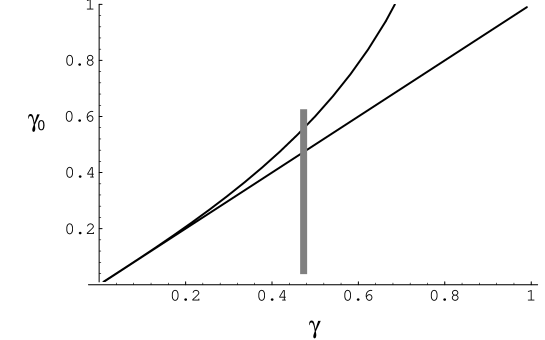
  Figure 1: a.$\gamma_{0}$ as a function of the ”renormalized” value $\gamma$; The grey band corresponds to the average value of $\gamma_{0}$ at LEP.

• Running coupling constant

  Let us now reconsider equation (8) when $\alpha_{s}$ is running. One has:

  $$\gamma_{0}^{2}\ =\ 4N_{c}{\alpha_{s}(Q)\over 2\pi}\ =\ {c_{0}^{2}\over\log{(Q/\Lambda)}}\ ;\ \ c_{0}\ =\ \frac{6}{\sqrt{33-2n_{f}}},$$

  where $n_{f}$ is the number of flavors ($n_{f}$ = 5 at LEP). The solution of Eq.(8) is of the form $N(Q)=N_{0}\exp{\Big{(}2c\sqrt{\log(Q)}\Big{)}}$, where $c$ is a constant. Using the following general identity,

  $$N(Qf(x))/N(Q)\simeq\exp{\Big{(}2c\sqrt{\log{Qf(x)/\Lambda}}-2c\sqrt{\log{Q/\Lambda}}\Big{)}}$$

  $$\simeq\exp{\Big{(}c\ \log f(x)/\sqrt{\log{Q/\Lambda}}\Big{)}}\ =\ \left[f(x)\right]^{\ c/\sqrt{\log{Q/\Lambda}}}.$$ (11)

  one obtains from Eq.(8):

  $$N(Q)\simeq N_{0}\exp{\Big{(}2c\sqrt{\log{Q/\Lambda}}\Big{)}}$$

  $$c^{2}\simeq c_{0}^{2}\left(1-\chi{(\gamma)}\right),$$ (12)

  where $\gamma\equiv c/\sqrt{\log{Q/\Lambda}}.$ As already pointed out, $\chi(\gamma)\simeq\gamma^{2}$ when $\gamma$ is small, that is the EC effect on the exponent of the mean multiplicity is a non-leading correction. However, as in the frozen coupling case, it ”renormalizes” the behaviour of the multiplicity.

2.2 The global second moment

If one goes to the second derivative of equation (7), one obtains the evolution equation for the global factorial moment, $I\!\!F_{2}$ :

$$\frac{\partial I\!\!F_{2}(Q)}{\partial\log(Q)}\ =\ \int_{0}^{1}\gamma_{0}^{2}\frac{dx}{x}\left(I\!\!F_{2}(Qx)+2N(Qx)N(Q(1-x))+I\!\!F_{2}(Q(1-x))-I\!\!F_{2}(Q)\right).$$ (13)

The way of dealing with this equation is to assume that $I\!\!F_{2}(Q)/N^{2}(Q)$ is a slowly varying function of $Q.$ This property, which is one of the KNO scaling relations $I\!\!F_{q}(Q)\propto N^{q}(Q),$ is known to be correct for the moments predicted by QCD[5]. Using this structure together with the power-like behaviour of $N$, (see Eq. (9)) gives :

$$I\!\!F_{2}=\left(\frac{2\Gamma^{2}(\gamma)}{\gamma\Gamma(2\gamma)(3+\chi(2\gamma)-4\chi(\gamma))}\right)\left(N(Q)\right)^{2}.$$ (14)

The result is displayed on Fig.2. The EC effects are clearly seen as a serious damping of the KNO ratio $I\!\!F_{2}/N^{2}$.

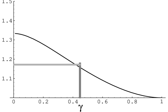
Figure 2: $I\!\!F_{2}$ as a function of $\gamma$. The DLA result (4/3) is obtained when $\gamma\to 0$. The vertical grey band is for $\gamma_{0}$ at LEP , while the horizontal one corresponds to the experimental value quoted in ref. [7] for one jet (in the forward hemisphere).

The running of the coupling constant does not modify the result which is very close to the experimental data[7] ($|bigf_{2}$ in one hemisphere). One notices that Eq. (14) leads to a weak violation of KNO scaling due to the dependence of $\gamma$ on $Q.$

3 The Local Jet multiplicity distribution

Let us come now to the main topics of our paper, namely the computation of the local correlations between partons. The characteristic feature of the jet multiplicity structure is that the evolution equation for the local density of partons is linear. It can be deduced from the branching structure of jet fragmentation in QCD.

Let us denote by $H(u,Q)$ the generating function for the density of factorial moments:

$$H_{q}\equiv\frac{\partial^{q}H}{\partial u^{q}}\Big{|}_{u=1}\ =\ \frac{{F}_{q}(\Delta)}{\Delta}\equiv\frac{{\mbox{$\langle n(n-1)..(n-q+1)\rangle$}}_{\Delta}}{\Delta}.$$ (15)

The QCD evolution equation of the multiplicity in an observation window of size $\theta$ pointing in a definite direction $\theta_{0}$ from the jet axis is schematically described in the figure. there are 2 contributions, one coming from the parton with a fraction $x$ of the available energy, the other coming from the branch of the fragmentation process with $1-x.$ Once substracted the variation of the phase-space from $\theta_{0}$ to $\theta$ by defining moments of the density as in Eq.(15), the only evolution comes from the energy degradation along the branch. In the DLA approximation, only one branch contributes to the hadron density evolution, since one parton keeps essentially undisturbed by the branching. In the EC case where we do not neglect the recoil effect, the two branches contribute. Note that one has to take into account the corresponding loss of virtuality $Qx$ and $Q(1-x)$ respectively. One obtains :

$$\displaystyle{\frac{\partial H(u,Q)}{\partial t}} \ =\ \int_{0}^{1}\gamma_{0}^{2}\ \frac{dx}{x}\Big{|}_{+}\left(H(u,Qx)+H(u,Q(1-x))\right)$$ (16)

$$\ =\ \int_{0}^{1}\gamma_{0}^{2}\ \frac{dx}{x}\left(\left[H(u,Qx)-1\right]+\left[H(u,Q(1-x))-H(u,Q)\right]\right)$$

where $\log{\theta_{0}/\theta}\equiv t$ plays the rôle of the evolution parameter and the phase-space splitting depends on the dimensionality, namely $\Delta\propto\theta^{d}$. One branch of the iteration contributes to $H(u,Qx)$ and the other to $H(u,Q(1-x))$ in the integrand, while the negative contributions are necessary to ensure the finiteness and unitarity conditions, namely $H(1,Q)\equiv 1$ and $\sum_{\Delta}{\partial H(u,Q)}/{\partial u}\big{|}_{u=1}=\sum_{\Delta}F_{1}(\Delta)\equiv N(Q).$

The solution of Eq.(16) is obtained by using the KNO scaling property of the multiplicity distribution inside a cone of fixed angular aperture $\theta$. In terms of the generating function $H$, it writes:

$$H(u,\lambda Q)\ =\ H(uN(Q\lambda)/N(Q),Q)$$ (17)

Inserting the property (17) into Eq.(16), and performing the $q^{th}$ derivative, one gets:

$$\frac{\partial H_{q}}{\partial t}\ =\ H_{q}\ \int_{0}^{1}\gamma_{0}^{2}\frac{dx}{x}\left(\left({\frac{N(Qx)}{N(Q)}}\right)^{q}+\ \left({\frac{N(Q(1-x))}{N(Q)}}\right)^{q}-1\right)$$

$$\ =\ H_{q}\ \int_{0}^{1}\gamma_{0}^{2}\frac{dx}{x}\left(x^{q\gamma}+\ (1-x)^{q\gamma}-1\right),$$ (18)

where we have used Eq.(• ‣ 2.1). Notice that Eq. (16), as well as (7), can be understood in terms of classical fragmentation models[2]. The connection between the present formalism and classical fragmentation is also a consequence of the KNO relation (17).

As a check of this procedure, let us recover the known results of the DLA approximation[2]. Neglecting the EC terms in Eq.(16), one obtains :

$$\frac{\partial H(u,Q)}{\partial t}\ =\ \int_{0}^{1}\gamma_{0}^{2}\ \frac{dx}{x}\left(H(u,Qx)-1\right),$$ (19)

from wich one obtains the fractal dimensions (2),(4).

3.1 Frozen coupling

Equation (18) reads :

$$\frac{1}{H_{q}}\frac{\partial H_{q}}{\partial t}\ =\ {\gamma_{0}^{2}}\ \frac{(1-\chi(q\gamma))}{q\gamma}\ =\ \frac{\gamma}{q}\ \frac{1-\chi(q\gamma)}{1-\chi(\gamma)}$$ (20)

where one makes use of relation(10). The corresponding corrections to the normalized factorial moments (1) and their fractal dimensions can be worked out :

$${\cal D}_{q}\ =\ \frac{\gamma}{q}\left[1+q+\frac{\chi(\gamma)-\chi(q\gamma)}{1-q}\right],$$ (21)

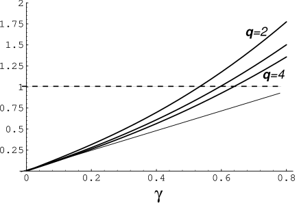
Figure 3: The multifractal dimensions ${\cal D}_{2},{\cal D}_{3},{\cal D}_{4}$ as functions of the coupling $\gamma$; The straight line is the DLA result for ${\cal D}_{4}$ as an example(2). The saturation limit is the dotted line at $d=1$ .

Notice that, while the correction to the unnormalized factorial moments, see Eq. (21), is a factor of order $(1-q^{2}\gamma^{2})/(1-\gamma^{2})$ in the exponent and can be important, the normalized ones are less sensitive to EC corrections. Since $\chi(\gamma)\simeq\gamma^{2}$ up to $\gamma\simeq 1.5$, the fractal dimension (20) reads

$${\cal D}_{q}\simeq\frac{\gamma(1+\gamma^{2})(q+1)}{q},\ \ q\gamma<1.5,$$ (22)

leading to an enhancement factor with respect to the multiplicity exponent at the same order ($\alpha_{s}^{3/2}$). However, when $q\gamma>1.5,$ the modification becomes more important and $q-$dependent. One observes an important increase of the fractal dimension, see Fig.3.

3.2 Running coupling

Let us consider again Eqs.(18), (20) with $\gamma_{0}$ defined with the running coupling and $\gamma$ as in formula (• ‣ 2.1). Neglecting both the variation of the coupling in the EC correction factors (higher order terms) and the $x$-dependence of the coupling (this approximation have been shown to be quite right in the range ($z<.6$) in ref. [2]), one obtains :

$${\cal D}_{q}(z)\simeq\frac{\gamma}{q}\left[1+q+\frac{\chi(\gamma)-\chi(q\gamma)}{1-q}\right]\ \frac{2}{1+\sqrt{1-z}},$$ (23)

where $\gamma$ is expressed as in formula (10). Notice that the saturation effect is stronger due to the running of the coupling (see, e.g., Fig.4 for the one-dimensional case).

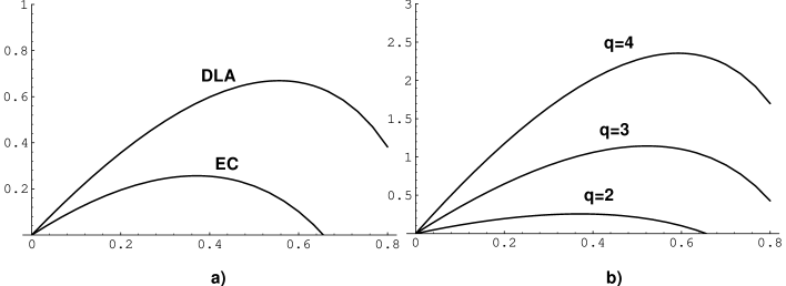
Figure 4: $\log[{\cal F}_{q}(z)/{\cal F}_{q}(0)]$, as a function of the scaling variable, $z=\log[\theta_{0}/\theta]/\log[E\theta_{0}/\Lambda]$. a: $q=3$, with and without EC corrections; b: $q=2$ (lower), $q=3$ and $q=4$ (upper), including EC corrections; the value $\gamma=.44$ is consistent with the LEP value of $\alpha_{s}$.

As a phenomenological application of our results, we perform a comparison of our predictions with experimental results, which while yet preliminary, have been presented as a first detailed analysis of correlations in a jet. As stressed in the experimental paper[13], the comparison of analytical QCD predictions with data on correlations is not easy due to the hadronization effects. The best candidate for a comparison is the study of particle correlations in a ring $\theta_{0}\pm\theta$ around the jet axis. The variation on $\theta$ allows one to obtain the dependence in $z,$ while considering as an observable the ratio $\log[{\cal F}_{q}(z)/{\cal F}_{q}(0)]$ minimizes the hadronization corrections[2].

The results are displayed on Fig. 5. The result of a Monte-Carlo simulation of the QCD parton cascade [11, *Cracow] is also shown on the same plot. The simulation is useful to take into account the corrections with respect to analytical calculations which occur when the parton cascade is correctly reproduced, e.g. overlap effects between angular domains, subasymptotic energy-momentum effects, hadronization effects (in part) etc…. For this comparison we make use of the following parameters : $\alpha_{s}(E\theta_{0})=.135$ for $\theta_{0}=25^{\circ}$(corresponding to $\alpha_{s}=.12$ for the whole jet with $Q_{0}=45$ Gev). This leads to $\gamma=.44$ or, from Eq.(10), $\gamma_{0}=.5$.

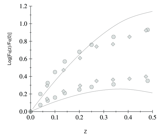
Figure 5: Phenomenological predictions for $\log[{\cal F}_{q}(z)/{\cal F}_{q}(0)]$ as a function of the scaling variable $z$. Upper curves,triangles and circles: $q=3$, lower ones $q=2$. Continuous lines: the analytical calculations from 4; circles: Preliminary Delphi data from Ref.[13]; squares: Numerical data from the Monte-Carlo simulation[11, *Cracow]

The analytical QCD predictions happen to be in reasonable agreement with both experimental results and numerical Monte-Carlo simulations, taken into account the approximations considered in the calculation. In particular, some bending of the factorial moments at small aperture angle $\theta$ is qualitatively reproduced. This effect is a typical predictions of the running coupling scheme, which is thus favoured by the data with respect to the frozen coupling case.

The full study of hadronization effects remain to be done. However, we may notice that when the slope of the intermittency indices (Fig. 4) goes to zero, the effective coupling $\gamma$ is around $1$ and one enters the not well known strong coupling regime of QCD. As a matter of fact, the only free parameter left in the Monte-Carlo simulation is the effective cut-off of the parton cascade i.e. the maximum value $\alpha_{s},\ \alpha_{0}$, one considers in the development of the parton branching process. In the example considered in the figure, we have found $\alpha_{0}\simeq.54,$ which is a quite reasonable value for switching on hadronization. All in all it is a positive fact that Local Parton-Hadron Duality seem to work reasonably for such refined quantities as correlations, once some caution is taken to minimize non-perturbative QCD corrections.

4 Conclusions

The Energy Momentum Conservation effects (or recoil effects) on the correlation properties of QCD jets are thus under some analytical control. The method proposed to handle these effects is the search for scaling solutions of the QCD generating function of local multiplicity density moments in angular phase-space. It is interesting to note the deep connection between the KNO-scaling[10] and the self-similar properties of correlations in the jet. This structure is reminiscent of general properties of fragmentation models and could be more fundamental than the level of approximation used to derive the result from QCD. Indeed, the same qualitative result is expected from the solution of the equation including EC terms plus other dominant next-to-leading effects (e.g. MLLA approximation scheme, see ref.([5])).

The phenomenological outcome of this study is that the analytical predictions come close to the experimental data and confirmed by the numerical simulation. Parton-Hadron duality for correlations seems to be supported provided hadronization effects can be minimized. Thus the self-similar structure of the QCD branching processes may eventually emerge from the background in the experimental analysis. Hadronization becomes dominant when the factorial moments bend and acquire a zero slope ($z\simeq 0.5$ in terms of the scaling variable of formula (5)). If one would insist to increase $z$ by reducing the opening angle of the detection window, one would find properties closer to soft processes, and thus difficult to predict theoretically.

From the theoretical point of view, the partial cancellation of EC corrections observed in the scaled factorial moments, leading to a moderate correction to the behaviour determined by the leading-log approximation, is a consistency check of the perturbative resummation predictions. Note however that this remark does not hold for moments of high rank $q\geq 4$, where a stronger correction is expected. The question remains to know whether this indicates a limitation of the perturbative calculations or the signal of a dynamical mechanism.

10

References

- [1] Y. Dokshitzer and I. Dremin, Nuclear Physics B402, 139 (1993)
- [2] P. Brax, J.-L. Meunier, and R. Peschanski, Zeit. Phys. C62, 649 (1994)
- [3] R. Peschanski, Multiparticle Dynamics 1992, World Scientific Ed., 1993
- [4] W. Ochs and J. Wosiek, Phys. Lett. B305, 144 (1993)
- [5] Y. Dokshitzer, V. Khoze, A. Mueller, and S. Troyan, Basics of Perturbative QCD, Editions Frontieres, Paris, 1991
- [6] Y. Dokshitzer, Phys. Lett. B305, 295 (1993)
- [7] P.D.Acton et al , OPAL, Zeit. Phys. C53, 539 (1992)
- [8] D. Decamp et al., ALEPH, Zeit. Phys. C53, 21 (1992)
- [9] P. Abreu et al., DELPHI, Nucl. Phys. B386, 417 (1992)
- [10] Z. Koba, H. Nielsen, and P. Olesen, Nucl. Phys. B40, 317 (1972)
- [11] P.Duclos and J.-L.Meunier, Zeit. Phys. C64, 295 (1994)
- [12] J.-L. Meunier, Soft Physics and Fluctuations, World Scientific Publishing Ed., 1993
- [13] F. Mandl, Multiparticle Dynamics 1994, World Scientific Ed., 1994