SUNY-NTG-95-20 A Mean Field Approach To The Instanton-Induced Effects Close To The QCD Phase Transition

Abstract

In the instanton models the chiral phase transition is driven by a transition from random instanton-antiinstanton liquid and correlated instanton-antiinstanton molecules. So far this phenomenon was studied by numerical simulations, while we develop alternative semi-analytic approach. For two massless quark flavors, both instantons and “molecules” generate specific 4-fermion effective interactions. After those are derived, we determine the temperature dependence of the thermodynamic quantities, the quark condensate and the fraction of molecules using standard mean field method. Using Bethe-Salpeter equation, we calculate T-dependence of mesonic correlation functions.

1 Introduction

The nature of the phase transition remains one of the main problems in non-perturbative QCD. Not only it is important to understand it from a theoretical point of view, but it is also the motivation for current and future heavy ion collision experiments. Major efforts are also being made to simulate finite-T QCD on the lattice, and many results have clarified to some extent the phase diagram of QCD-related theories, see reviews [1, 2].

At zero temperature the mechanism of spontaneous chiral symmetry breaking and even the very existence of most light hadrons is believed to be connected with the fermionic (quasi)zero modes generated by instantons. The specific instanton liquid model was suggested in [3], and then studied both analytically [4, 5] and numerically [6, 7, 8, 9, 10]. Even the simplest random model (RILM) was found to reproduce mesonic and baryonic correlation functions, known from phenomenology [11] and the lattice simulations [12]. Furthermore, the “instanton liquid” itself, with parameters closed to those predicted, were “distilled” from lattice configurations by cooling [13, 14].

However, it is much less firmly established what happens with instantons at finite temperature T. It has been known for a long time that at $high$ T the instanton density is suppressed by the Debye-type screening [15, 16], and it was thought first that it may be the reason for chiral symmetry restoration (see e.g. [17]). However both recent theoretical analysis at $low$ T [18] and numerical simulations [19], show that up to $T_{c}$ the instanton density changes are not significant, and therefore an instanton suppression hardly can be an explanation.

That is why another mechanism was studied in [20]: the phase transition may be driven by “pairing” of instantons and antiinstantons into $I\bar{I}$“molecules”. A two-component (or the so called “cocktail”) model was proposed, in which at $T<T_{c}$ individual instantons and “molecules” coexist in ensemble, while (for m=0) at $T>T_{c}$ only molecules survive and the chiral symmetry gets restored.

In [10] the Cocktail Model was studied numerically, by keeping the temperature fixed and changing the molecule fraction $f$. Many mesonic and baryonic correlation functions were calculated: they show very dramatic changes as $f$ goes from small values to 1. Furthermore, a very interesting hints for survival of some hadrons $above$ the phase transition were presented. This scenario of the phase transition was been recently confirmed by numerical simulations of the instanton vacuum at finite temperature in which both boson and fermion induced interaction between the pseudo-particles is taken into account [21]. It was shown that the molecules start to form only close to $T_{c}$, and that they are polarized in color space as well as in the Euclidean time direction, as anticipated in [9, 20].

In the present paper, we investigate the same two-component (or “cocktail”) model by different (analytic) methods. The main difference with numerical simulations mentioned above is that they first calculate quark propagation in a $given$ background field (a superposition of instantons), averaging over gauge fields $later$. In our approach we start with the integration over collective variables of instantons, deriving effective interaction between quarks. Basically, our next steps are the same as in the Bardeen-Cooper-Schreiffer theory of superconductivity or Numbu-Jona-Lasinio model of chiral symmetry breaking. Our 4-fermion interaction effective interaction is, however, much more complicated, it includes two types of nonlocal terms - one from the random instantons and antiinstantons, and the another one from the strongly correlated pairs, or molecules.

The paper is organized as follows:

In section 2 we calculate the effective interaction $S_{eff}$ and the overlap matrix element $T_{I\bar{I}}$, at temperature $T$, of an instanton and an anti-instanton in the most attractive relative orientation whose separation has only a time component (i.e. they lie on the Matsubara circle). After that we perform an integration over the 11 quasi-zero modes of the molecule to find the corresponding activity (or internal partition function of a molecule) $Z_{mol}$. We find out that the equilibrium configuration of the $I\bar{I}$ system, in the temperature range around $T_{c}$, is when the instanton and the anti-instanton are separated by the maximal interval in Matsubara time $\tau={1\over 2T}$, they have zero spatial separation and are in the most attractive orientation in color group.

In section 3, we evaluate the partition function, assuming that the fermion determinant is a product of the separate instanton, antiinstanton and molecule determinants. Next we exponentiate them, by performing an Inverse Laplace Transformation. Then we integrate over the instanton, antiinstanton and molecule positions to obtain an effective four-fermion lagrangian (we study the case of two flavors in the chiral limit).

In section 4, we use this Lagrangian in a Hartree-Fock approximation, leading to a theory of free fermions, but with temperature and momentum dependent mass. Then we calculate the free energy and minimize it in order to determine our parameters such as the molecule fraction $f$, the quark condensate and the Laplace parameters for the liquid and for the molecules. We solve four mean field equations and determine the temperature dependence of all parameters. The results clearly show the transition from instanton liquid to gas of molecules and the restoration of the chiral symmetry.

In section 5, we calculate mesonic correlation functions, using the Bethe- Salpeter equation. We also extract the pion-quark couplings, the pion decay constant $f_{\pi}$ and its coupling to pseudoscalar current $\lambda_{\pi}$. All the results naturally respect the Goldstone theorem (for example $f_{\pi}$ vanishes at $T=T_{c}$). To compare with the numerical simulations for the mesonic correlation functions, we perform a Fourier transform to Euclidean time. Reasonable agreement between them is observed.

2 The $I\bar{I}$ Molecules Around $T_{c}$

This section is relatively independent of the rest of the paper in the sense that it deals with properties of the $single$ $I\bar{I}$ molecule. It consists of two steps: the first is a new calculation of the $\bar{I}I$ interaction in the relevant configuration (so to say, the quantum mechanics of it); while the second deals with its internal statistical mechanics. In the next sections we will proceed to the statistical ensemble of $multiple$ instantons around the critical temperature.

The $I\bar{I}$ interaction and the overlap matrix elements of the fermionic zero modes, both at zero and at finite temperature, were studied in detail in [22, 23]. Unfortunately these studies were not complete in the sense that they did not include our region of interest – the configurations in which the pseudo-particles lie around the opposite ends of a diameter on the Matsubara circle.

The best definition of the $classical$ $I\bar{I}$ interaction $S_{int}=(S-2S_{0}),$ where $S_{0}$ is the single instanton action, is given by the so-called streamline configurations [24]. Unfortunately, at finite temperature, the conformal symmetry that allows to find the streamline is missing. Therefore, one has to use some ansatz for the $I\bar{I}$ configuration which has a natural extension to non-zero T. We are going to use the ratio ansatz [6]

$$A^{a}_{\mu}(x)=-{1\over g}{O^{ab}_{I}\bar{\eta}^{b}_{\mu\nu}\partial_{\nu}\Pi_{I}+O^{ab}_{\bar{I}}\eta^{b}_{\mu\nu}\partial_{\nu}\Pi_{\bar{I}}\over\Pi_{I}+\Pi_{\bar{I}}-1},$$ (1)

where $\Pi_{I}=\Pi(x-z_{I}),$ $\Pi_{\bar{I}}=\Pi(x-z_{\bar{I}})$ and

$$\Pi({\bf r},t)=1+{\pi T\rho^{2}\over r}{\sinh(2\pi rT)\over\cosh(2\pi rT)-\cos(2\pi tT)},$$ (2)

which is free from the artifacts of the sum ansatz and provides a reasonable repulsive core. The classical bosonic interaction is just obtained from this expression, by numerical calculation of the classical action.

The quark-induced interaction is described in general by fermionic zero-mode overlap matrix element:

$$T_{I\bar{I}}=\int dtd^{3}{\bf x}\phi_{I}^{\dagger}(x-z_{I})\not\!\!D\phi_{\bar{I}}(x-z_{\bar{I}}),$$ (3)

In this case we use the simplest sum ansatz [25], because in this case one can use an ordinary derivative instead of a covariant one. As it was shown in [22], the results in this case differ insignificantly from the ones obtained by the ratio ansatz.

The $O(3)$ symmetry of the $I\bar{I}$ configuration along the Matsubara circle allows us to reduce the above integral and the integral for the bosonic part of the action to a two dimensional one, and we perform the integration numerically. Our results coincide with the ones from [22, 23] in the region where their formulas are valid (for Matsubara time separations that are not close to $L/2={1\over 2T}$). The results for $T_{I\bar{I}}$ are shown in Fig. 1 (a), and the combined $e^{-S_{int}}T^{4}_{I\bar{I}}$ in Fig. 1 (b) (the dotted line).

The second step is to include the “internal entropy”, or multiplicity of different $I\bar{I}$ configurations into account. One has to take the integral

$$Z_{mol}(T)=\int d^{11}\Omega\ T^{2N_{f}}_{I\bar{I}}e^{-S_{int}}$$ (4)

over all collective variables. These are the time separation $\tau$, the three dimensional spatial separation and, for $SU(3)$, seven relative orientation angles. Most of the 11-dimensional integral, however, can be done by a saddle-point approximation. Both $S_{int}$ and $T_{I\bar{I}}$ decay exponentially in the spatial separation directions. The second derivatives of $S_{int}$ over orientation angles are big, because they are multiplied by $8\pi^{2}/g^{2}=S_{0}\sim 10>>1$. In contrast to that, the angular dependence of $-2N_{f}\ln(T_{I\bar{I}})$ is rather weak, so in angular integrals we treat $T_{I\bar{I}}$ as a constant. Finally, we find that the saddle point approximation is not good at all for the integral along the time separation $\tau$ . That is why we perform this last integration explicitly.

In Fig. 1 (b), we show the time dependence of the integrand $Z_{mol}^{\prime}(\tau)=\int d^{10}\Omega\ T^{4}_{I\bar{I}}e^{-S_{int}}$, (the integration over all variables but the Matsubara time), at $T_{c}$, compared to the exponent of the classical and quark- induced interaction $\exp-\{S_{int}-2N_{f}\ln(T_{I\bar{I}})\}$, which has a maximum at about $\tau=L/4$ and a minimum at $\tau=L/2$. One can see that when the multiplicity of phase space is included, the $I\bar{I}$ molecules are distributed around $\tau=1/2T$. The corresponding time dependence of $T_{I\bar{I}}$ at $T_{c}$, which is is shown in Fig. 1(a), is rather weak around the maximum of $Z^{\prime}$. This allows us to use its central value for all molecules that participate in our “cocktail model”. After the last integral is done, one gets the absolute value of the statistical sum for molecules $Z_{mol}$. The temperature dependence of $Z_{mol}$ and $T_{I\bar{I}}$ is shown in Figs. 1 (c), (d).

How accurate is our saddle point integration? In the next section we will find that in order to set the phase transition at $T_{c}=150MeV$ one needs $Z_{mol}$ about 1.8 larger: it means only a $5\%-10\%$ error per integration over each of the $I\bar{I}$ collective parameters. However, we think real uncertainty in $Z_{mol}$ is larger, and it is about one order of magnitude (as one can judge from including $-4\ln(T_{I\bar{I}})$ in the second derivative over the orientation parameters, etc). Nevertheless we think its temperature dependence is evaluated reliably, and we use it below in our calculation of the thermodynamical properties of the instanton ensemble , the correlation functions and the pion coupling constants.

3 Effective 4-Fermion Interaction

Let us start with a list of assumptions and simplifications, defining the model and the particular parametrization used. We emphasize, that most of them are possible only because we are primarily interested in a comparatively narrow interval of temperature T around $T_{c}$, in which significant structural changes (the phase transition) takes place.

• We fix the total pseudo-particle density to be a constant for T up to $T_{c}=150MeV$, with only composition $f$ changing. We take $n_{t}=1fm^{-4}$ specifically, lacking more accurate number. (None of the results change qualitatively if, say, it is modified by a factor of 2.)

• Lattice data in [19] indicate, that the instanton radius doesn’t change much with $T$ till well above the phase transition. So we also fix it at $\rho=0.34fm$. (However we are going to express all dimensional quantities in units of $\rho$ and its powers anyway.)

• In the previous section we have shown that the dominant configuration for the $I\bar{I}$ molecules is the one, in which the distance between their centers in the Euclidean time direction is equal to “half-box” $R=L/2\equiv 1/2T$, the spatial distance is 0, and they have the most attractive relative orientation in color space. Although the molecule distribution has some span around $L/2$ in the time direction, $T_{I\bar{I}}$ changes little, which allows us to use one value of it for all molecules.

• $T_{c}$ and $S_{0}$ are related by the requirement that all unpaired instantons disappear at $T_{c}$. This condition can be satisfied only in a window around $T_{c}=150Mev$. We use the following values: $T_{c}=150MeV,S_{0}=9.5$. However there is a big uncertainty in this relation, due to the uncertainty of the calculated value of the molecule activity $z$.

• We are going to ignore all bosonic and fermionic interactions between random instantons and among $I\bar{I}$ molecules.

Now we proceed to calculation of the effective quark interaction. For one instanton it is the well known ’t Hooft effective interaction. It can be derived from the zero-mode part of the quark propagator :

$$S(x,y)=S_{NZM}(x,y)+{\phi_{I}(x-z_{I})\phi^{\dagger}_{I}(y-z_{I})\over-im},$$ (5)

where $\phi(x)$ is the quark zero mode in the field of an instanton with center at $z_{I}$ and $S_{NZM}(x,y)$ represent contributions of non-zero modes, (following [4] we shall approximate these contributions by the free quark propagator $S_{0}$). For $N_{f}$ light fermions, one should take the corresponding power of $S(x,y)$, multiply it with the instanton probability (P$\sim m^{N_{f}}$) and then cancel m in both, resulting in the interaction which is finite in the chiral limit (m=0).

Similar procedure can be repeated for an isolated $I\bar{I}$ molecule [21]. In the chiral limit quarks have the following propagator:

$$S_{m}(x,y)=S_{0}(x,y)+{\phi_{I(m)}(x-(z_{m}-L/4))\phi^{\dagger}_{\bar{I}(m)}(y-(z_{m}+L/4))\over T_{I\bar{I}}}+$$ (6)

$${\phi_{\bar{I}(m)}(x-(z_{m}+L/4))\phi^{\dagger}_{I(m)}(y-(z_{m}-L/4))\over T_{I\bar{I}}},$$ (7)

where $T_{I\bar{I}}$ was defined in (2).

For $N_{f}=2,$ the following fermionic path integral generates the above propagators:

$$Z=\int d\psi d\psi^{\dagger}{\exp\{\int d^{4}x\psi^{\dagger}i\not\!\partial\psi\}\over N_{+}!N_{-}!N_{m}!}\prod_{I=1}^{N_{+}}c_{\rho}\theta_{+}\prod_{\bar{I}=1}^{N_{-}}c_{\rho}\theta_{-}\prod_{m=1}^{N_{m}}c_{\rho}^{2}c\theta_{m},$$ (8)

where

$$\theta_{+}=\int dz_{I}d\Omega_{I}\prod_{f=1}^{2}\big{(}\int d^{4}x\psi^{\dagger}_{f}(x)i\not\!\partial\phi_{I}(x-z_{I})\int d^{4}y\phi_{I}^{\dagger}(y-z_{I})i\not\!\partial\psi_{f}(y)\big{)},$$ (9)

$$\theta_{-}=\int dz_{\bar{I}}d\Omega_{\bar{I}}\prod_{f=1}^{2}\big{(}\int d^{4}x\psi^{\dagger}_{f}(x)i\not\!\partial\phi_{\bar{I}}(x-z_{\bar{I}})\int d^{4}y\phi_{\bar{I}}^{\dagger}(y-z_{\bar{I}})i\not\!\partial\psi_{f}(y)\big{)},$$ (10)

$$\theta_{m}=\int dz_{m}d\Omega_{m}\Big{[}\prod_{f=1}^{2}\Big{(}T_{I\bar{I}}+\int d^{4}x\psi^{\dagger}_{f}(x)i\not\!\partial\phi_{I(m)}(x-z_{m}+{L\over 4})\times\qquad\qquad\quad\$$ (11)

$$\int d^{4}y\phi_{\bar{I}(m)}^{\dagger}(y-z_{m}-{L\over 4})i\not\!\partial\psi_{f}(y)+\int d^{4}x\psi^{\dagger}_{f}(x)i\not\!\partial\phi_{\bar{I}(m)}(x-z_{m}-{L\over 4})\times$$ (12)

$$\int d^{4}y\phi_{I(m)}^{\dagger}(y-z_{m}+{L\over 4})i\not\!\partial\psi_{f}(y)\Big{)}+\sum_{f=1}^{2}\Big{(}\int d^{4}x\psi^{\dagger}_{f}(x)i\not\!\partial\phi_{I(m)}(x-z_{m}+{L\over 4})\times$$ (13)

$$\int d^{4}y\phi_{I(m)}^{\dagger}(y-z_{m}+{L\over 4})i\not\!\partial\psi_{f}(y)\int d^{4}x^{\prime}\psi^{\dagger}_{f}(x^{\prime})i\not\!\partial\phi_{\bar{I}(m)}(x^{\prime}-z_{m}-{L\over 4})\times$$ (14)

$$\int d^{4}y^{\prime}\phi_{\bar{I}(m)}^{\dagger}(y^{\prime}-z_{m}-{L\over 4})i\not\!\partial\psi_{f}(y^{\prime})\Big{)}\Big{]},$$ (15)

Note, that there are no odd terms in $T_{I\bar{I}}$, because of the integration over $\Omega_{m}$. Here $z_{i}$ and $\Omega_{k}$ are the collective coordinates of an $I\bar{I}$ molecule, $c=Z_{mol}/T_{I\bar{I}}^{2}$ and $c_{\rho}$ is the single instanton partition function [28] integrated over the instanton radius $\rho$. The convergence of the latter is due to the non-perturbative $g(\rho)$, which tends to a constant for large $\rho$ [14, 34].

Now, applying inverse Laplace Transformation, we get the following partition function:

$$Z=const\int d\beta_{+}d\beta_{-}d\beta_{m}\exp\{-(N_{+}+1)\log(\beta_{+}/c_{\rho})-(N_{-}+1)\log(\beta_{-}/c_{\rho})$$ (16)

$$-(N_{m}+1)\log(\beta_{m}/(c_{\rho}^{2}c))+\int d^{4}x(\psi^{\dagger}i\not\!\partial\psi\ -\beta_{+}\theta_{+}+\beta_{-}\theta_{-}+\beta_{m}\theta_{m})\}.$$ (17)

To evaluate the effective interaction $\theta_{i}$ terms we go to momentum space and do the integrations over the orientation angles and the center coordinates of the instantons, antiinstantons and molecules. The Fourier transforms of the fermion zero modes at finite temperature are [29]:

$$\alpha({\bf k},\omega_{n})=({\bf k}^{2}+\omega_{n}^{2})(A^{2}+B^{2}),$$ (18)

$$A = {1\over 2\pi\rho}\int_{0}^{\infty}4\pi r^{2}dr\int_{0}^{1/T}dt\left({\cos(kr)\over kr}-{\sin(kr)\over k^{2}r^{2}}\right)\cos(\omega_{n}t)\Pi^{1/2}\times$$ (20)

$$\hbox{\hskip 180.67499pt}\partial_{r}\left({(\Pi-1)\over\Pi}{\cos\pi tT\over\cosh\pi rT}\right),$$

$$B = {1\over 2\pi\rho}\int_{0}^{\infty}4\pi r^{2}dr\int_{0}^{1/T}dt{\sin(kr)\over kr}\sin(\omega_{n}t)\Pi^{1/2}\partial_{r}\left({(\Pi-1)\over\Pi}{\cos\pi tT\over\cosh\pi rT}\right),$$ (21)

where $\Pi$ is the potential (2) that also appears in the finite temperature zero modes $\phi^{R}$ in coordinate space [30]:

$$\phi^{R}={1\over 2\pi\rho}\Pi^{1/2}\not\!\partial\left({(\Pi-1)\over\Pi}{\cos\pi tT\over\cosh\pi rT}\right){\bf\epsilon}^{R},$$ (22)

and ${\bf\epsilon}^{R}$ is the standard constant spinor coupling spinor and Dirac indexes. Combining all fermion terms together, one obtains the following nonlocal four-fermion interaction :

$$S_{4f}=\int\prod_{i=1}^{4}{d^{4}k_{i}\over(2\pi)^{4}}(2\pi)^{4}\delta^{4}(k_{1}-k_{2}+k_{3}-k_{4})\sqrt{\alpha(k_{1})\alpha(k_{2})}\times$$ (23)

$$\sqrt{\alpha(k_{3})\alpha(k_{4})}\Big{\{}(\beta_{+}+\beta_{-}){1\over 16N_{c}^{2}}\left[(\psi^{\dagger}\tau^{-}_{a}\psi)^{2}-(\psi^{\dagger}\tau^{-}_{a}i\gamma_{5}\psi)^{2}+octet\ terms\right]-$$ (24)

$$\beta_{m}\bigg{[}{1\over 4N_{c}^{2}}\left((\psi^{\dagger}\tau_{a}\psi)^{2}+(\psi^{\dagger}\tau_{a}i\gamma_{5}\psi)^{2}\right)-{1\over 4N_{c}^{2}}\left((\psi^{\dagger}\tau_{a}\gamma_{0}\psi)^{2}+(\psi^{\dagger}\tau_{a}\gamma_{0}\gamma_{5}\psi)^{2}\right)+$$ (25)

$${1\over N_{c}^{2}}(\psi^{\dagger}\gamma_{0}\gamma_{5}\psi)^{2}+octet\ terms\bigg{]}\Big{\}},$$ (26)

where $\tau^{-}_{a}=(i,{\bf\tau})$, while $\tau_{a}=(1,{\bf\tau})$. The four fermion interaction is given in a Fierz symmetric form, which means that all permutations of these terms are included. We have shown explicitly only the color singlet terms. The last square brackets is the “molecular interaction” derived in [21]. There are no two-fermion terms, because the integral over the orientation of the molecule in color space is zero.

One can view this Lagrangian is a variant of the (nonlocal) Nambu-Jona-Lasinio model at finite temperature, with particular coefficients and with a natural cutoff given by the nonlocality of the vertices, at a scale $1/\rho$. We can now treat this interaction analogously to refs. [31, 32] for the NJL model.

4 The Mean Field Approximation and Thermodynamics

To calculate the thermodynamic properties of the system, we first bosonize the fermionic action, making Hubbard-Stratonovitch transformation,

$$\sqrt{\prod\alpha(k_{i})}(\psi^{\dagger}\psi)^{2}\to 2\sqrt{\alpha(k_{1})\alpha(k_{2})}\psi^{\dagger}(k_{1})\psi(k_{2})V_{4}(2\pi)^{4}\delta^{4}(k_{3}-k_{4})Q-$$ (27)

$$V^{2}_{4}(2\pi)^{8}\delta^{4}(k_{1}-k_{2})\delta^{4}(k_{3}-k_{4})Q^{2}.$$ (28)

Then we consider the bosonic field $Q$ as a constant, to be determined from free energy minimization. As there is no net topological charge, $\beta_{+}=\beta_{-}=\beta,$. We also define $f={2N_{m}\over N_{tot}},N_{+}=N_{-}={1-f\over 2}n_{tot}V_{4},N_{m}={f\over 2}n_{tot}V_{4}.$ After integration over the fermion degrees of freedom we have the following free energy:

$${\Delta F\over V_{4}}=-T^{2}_{I\bar{I}}\beta_{m}+(1-f)n_{tot}\log({\beta\over c_{\rho}})+{f\over 2}n_{tot}\log({\beta_{m}\over c_{\rho}^{2}c})+{Q^{2}\over 8N_{c}^{2}}(\beta+2\beta_{m})-$$ (29)

$$4N_{c}\int{d^{4}k\over(2\pi)^{4}}\log(k^{2}+M^{2}(k)),$$ (30)

where one can identify the chemical potentials for the “liquid” component $\log({\beta\over c_{\rho}})$ and for the “molecular” one $\log({\beta_{m}\over c_{\rho}}c),$. The last term corresponding to a gas of massive quarks with the (instanton-induced) momentum-dependent mass

$$M(k)={\alpha(k)Q(\beta+2\beta_{m})\over 4N_{c}^{2}}$$ (31)

We shall determine this mass from a self-consistency condition, represented graphically in Fig. 2 (a), where the vertex K is a sum of the instanton and the molecular interactions (Fig. 2 (b)).

Our next step is minimization of $\Delta F$ with respect to $f,\beta_{m},\beta,Q.$ There are four equations:

$$\beta_{m}-c\beta^{2} = 0,$$ (32)

$$T^{2}_{I\bar{I}}-{fn_{tot}\over 2\beta_{m}}+8N_{c}\int{d^{4}k\over(2\pi)^{4}}{2M(k)\over k^{2}+M^{2}(k)}{Q\alpha(k)\over 4N_{c}^{2}}-{Q^{2}\over 4N_{c}^{2}} = 0,$$ (33)

$$-{(1-f)n_{tot}\over\beta}+4N_{c}\int{d^{4}k\over(2\pi)^{4}}{2M(k)\over k^{2}+M^{2}(k)}{Q\alpha(k)\over 4N_{c}^{2}}-{Q^{2}\over 8N_{c}^{2}} = 0,$$ (34)

$$4N_{c}\int{d^{4}k\over(2\pi)^{4}}{2M(k)\over k^{2}+M^{2}(k)}{\alpha(k)\over 4N_{c}^{2}}-{2Q\over 8N_{c}^{2}} = 0.$$ (35)

One can notice, that the first equation is the condition for chemical equilibrium between the random and molecular components. These four equations can be reduced to one “gap” equation, that has to be solved numerically:

$${1\over N_{c}}\int{d^{4}k\over(2\pi)^{4}}{(1+2c\beta)\alpha^{2}(k)\over k^{2}+(1+2c\beta)^{2}(1-f)n_{tot}\alpha^{2}(k)/(2N_{c}^{2})}=1,$$ (36)

with:

$$\beta=\big{[}-(1-f)n_{tot}+\sqrt{(1-f)^{2}n_{tot}^{2}+f/(2c)n_{tot}T_{I\bar{I}}^{2}}\big{]}{1\over T_{I\bar{I}}^{2}}.$$ (37)

At $T_{c}$, all unpaired instantons disappear $(f\to 1)$ and the chiral symmetry is restored. The condition $f=1$ is satisfied on a line in the $T,S_{0}$ plane . We have chosen $T_{c}=150MeV=0.26/\rho$ and $S_{0}=9.5$. Of course, when $f=1$ or $f=0,$ the saddle point approximation for the $\beta$ integrals is no longer valid, so our model is restricted in the region $0<f<1,$ where the saddle point method is justified in the thermodynamic limit $V_{4}\to\infty.$ We see that when $f\to 1$, $\beta_{m}=1/2n_{tot}/(iT_{I\bar{I}})^{2},$ $\beta=\sqrt{n_{tot}/(2c(iT_{I\bar{I}})^{2})}$ does not tend to 0, so that the $U_{A}(1)$ symmetry remains broken when $T\to T_{c}$. This can be seen also in our discussion of the correlation functions in section 4.

Our results are presented in Fig.3, where the molecule fraction $f$, the effective quark mass $M({\bf 0},\pi T)$, the quark condensate $\langle\bar{\psi}\psi\rangle$ and the energy density $\epsilon$ are presented. Note, that the local $\langle\bar{\psi}\psi\rangle$ has one power of the formfactor $\alpha$ less under the momentum integral, compared to the nonlocal mean field $Q$. $\langle\bar{\psi}\psi\rangle$ is normalized to the phenomenological value of the quark condensate at $T=0$. We see that in about $20MeV$ the fraction of the molecules drops to about half, the quark condensate almost reaches its phenomenological value at $T=0$, but the constituent quark mass, which is defined as the value of the momentum dependant mass from the gap equation at zero spatial momentum and Matsubara frequency $\pi T$, is still low – about 1/3 of its phenomenological value at $T=0$. (The reader should be warned that one can hardly compare the mass value obtained in the present calculation with the usual constituent quark mass $M(\vec{k}=0,\omega=0)\sim 350MeV$ because the minimal energy possible $\omega\approx\pi T_{c}$ is rather large.) In addition, the finite temperature formfactors have a maximum at spatial momentum ${\bf k}_{max}\not=0$, so we show with a dotted line the temperature dependence of the mass defined at $k=({\bf k}_{max},\pi T)$.

This behaviour of the thermodynamic quantities looks similar to the one obtained in [29] or in the NJL models [32], and both are governed by similar gap equations for the constituent quark mass or the quark condensate. However the physics of the transition in our case is quite different. In [32] the transition is governed by the suppression of the quark condensate by thermal excitations of quarks. In [29] there is an additional thermal suppression of the instanton density, which results in additional suppression of the effective coupling constant. In our case, the main effect is the reorganization of the instanton vacuum: it leads to reorganization of the Lagrangian by itself. This can be seen by the fact that the mean field $Q$ (a $nonlocal$ analogue of the quark condensate), is proportional to square root of the density of the random component $1-f$. Our mechanism makes the transition region narrower and the transition temperature $T_{c}$ lower.

In Fig. 4 (a) we show the pressure $p=-\Delta F$ (the solid line), together with its different components: pressure of free massless fermions $4N_{c}\int{d^{4}k\over(2\pi)^{4}}\log(k^{2})$ (open triangles), the deviation from it, due to the effective mass $4N_{c}\int{d^{4}k\over(2\pi)^{4}}\log({k^{2}+M^{2}(k)\over k^{2}})$ (open squares), the contribution from the condensate $-{Q^{2}\over 8N_{c}^{2}}(\beta+2\beta_{m})$ (stars), the contributions from the molecules $T^{2}_{I\bar{I}}\beta_{m}-{f\over 2}n_{tot}\log({\beta_{m}\over c_{\rho}^{2}c})$ (black squares), and the instanton liquid $-(1-f)n_{tot}\log({\beta\over c_{\rho}})$ (black triangles). For comparison,we also show that the pressure of a pionic gas $p=0.987T^{4}$ (the dotted line) is significantly smaller than any of the components under consideration, and thus unimportant.

In Fig. 4.(b) the energy density $\epsilon$ below the phase transition point is shown to be actually directly proportional to the molecule fraction $f$. This correlates well with the observation made in [21], that (unlike the individual instantons) the molecules have a net positive energy, even in the classical approximation.

5 Mesonic Correlation Functions

Our last step is investigation of the effect of the 4-fermion effective interaction on mesonic spectra at $T\approx T_{c}$. Using Bethe-Salpeter equation one may calculate mesonic corelation functions, similarly to what was done in [31, 32]. Our major advantage is that we naturally have a non-local vertices, which provide an ultraviolet cutoff. We start with the two-body interaction kernel K, which is given by the four-fermion terms in the effective lagrangian. Then we have the BS equation for the quark-antiquark T matrix(Fig. 2 c) (See also Fig. 2 (c)):

$${\cal T}(q)={\cal K}+i{\rm Tr}\int{d^{4}P\over(2\pi)^{4}}\alpha(p+{q\over 2})\alpha(p-{q\over 2})[{\cal K}S_{F}(p+{q\over 2}){\cal T}(q)S_{F}(p-{q\over 2})].$$ (38)

The trace is taken over the Dirac, flavour and color matrices. For the colorless meson channels we need only the color singlet terms in the lagrangian. Then using the symmetries of the Matsubara space-time, we can decompose T and K into covariant structures.

$$\langle\bar{q}_{4}q_{3}|{\cal K}|\bar{q}_{2}q_{1}\rangle=\sum_{i,\alpha}K^{i}_{\alpha}\left[\Gamma_{\alpha}{\tau^{i}\over 2}\right]_{34}\left[\Gamma_{\alpha}{\tau^{i}\over 2}\right]_{12},$$ (39)

where $\Gamma\alpha$ denotes Dirac tensors.

Because at $T\not=0$ there is less symmetry than at zero temperature, we have more structures. However our particular action (15) contains only scalar and pseudoscalar terms and the time oriented vector and axial terms, produced by $\gamma_{0}$ and$\gamma_{0}\gamma_{5}$, therefore only the following coefficients are non-zero:

$$K_{S}^{i} = {-1\over 4N_{c}^{2}}[2\beta_{m}+2(\delta_{i0}-{1\over 2})\beta],$$ (40)

$$K_{P}^{i} = {1\over 4N_{c}^{2}}[-2\beta_{m}+2(\delta_{i0}-{1\over 2})\beta],$$ (41)

$$K_{V}^{i} = {1\over 2N_{c}^{2}}\beta_{m},$$ (42)

$$K_{A}^{i} = {1\over 2N_{c}^{2}}(1-4\delta_{i0})\beta_{m}$$ (43)

If we define the loop integral:

$$J^{ij}_{\alpha\beta}(q)=iN_{c}\rm tr\int{d^{4}p\over(2\pi)^{4}}\alpha(p+{q\over 2})\alpha(p-{q\over 2})[\Gamma_{\alpha}{\tau^{i}\over 2}S_{F}(p+{q\over 2})\Gamma_{\beta}{\tau^{j}\over 2}S_{F}(p-{q\over 2})],$$ (44)

then the solution of the BS equation (in matrix notation) is:

$$T=[1-JT]^{-1}K.$$ (45)

To get the mesonic correlation function for the corresponding channel, we have to multiply T from the left and the right with two loop integrals $J$ (those have only two formfactors $\sqrt{\alpha}$, instead of four, because the correlation function is defined for point-like currents). For all channels, we have separated equations except for the pseudoscalar and axial vector channels which mix both for isospin 1 ($\pi$) and 0 ($\eta$). In Fig.5 we show the Fourier transforms of the correlation functions for Euclidean time separation of the currents, normalized to the free correlation function at finite temperature. We show them in 6 steps with $\Delta T\approx 9MeV$, starting from $T=150MeV$ and ending with $T\approx 105MeV$.

The most striking feature is the strong attraction in the pion channel, which remains robust and does not disappear at $T_{c}$. This is due mainly to the residual ’t Hooft interaction (induced by the propagating quarks) and in a lesser extent to the attractive character of the molecular interaction in this channel (triangles). This feature is in agreement with the lattice simulations around $T_{c}$ [33], which also show a strong pion signal beyond $T_{c}$. Futhermore, at $T_{c}$ our pion signal is similar to the one from the numerical simulations of the interacting instanton liquid [10], although stronger.

The results are in agreement with all chiral theorems, and they clearly show restoration of the chiral symmetry at $T_{c}$. In particular, at $T=T_{c}$ the $\pi$ pseudoscalar correlation function $\langle PP^{1}\rangle$ coincides with the $\sigma$ scalar correlation function $\langle SS^{0}\rangle$. Another feature in agreement with the chiral symmetry is that the pion is decoupled from the axial current $(f_{\pi}\to 0)$ at $T\to T_{c}$, but remains coupled to the pseudoscalar one $(\lambda_{\pi}\not=0)$ even in the pure molecular vacuum (f=1).

An open theoretical issue debated in the literature is how strongly the $U_{A}(1)$ chiral symmetry is violated at $T\sim T_{c}$, see e.g. [34, 35, 36, 37]. We remind that this symmetry is strongly broken by random liquid at $T=0$, but it is respected by the new term in the Lagrangian due to “molecules” which we derived above. Although molecules are prevailing above $T_{c}$ the ’t Hooft interaction does not disappear completely at any T. One way to explain it, is to say that external quarks induce additional instantons, absent in vacuum.

The way to measure $U_{A}(1)$-violating effects is to calculate the correlation function for $\eta$ (the isoscalar pseudoscalar) or the isovector scalar, to be referred to as $\delta$, and compare their properties with the pion or sigma ones. These two channels are $U_{A}(1)$ partners of $\sigma$ and $\pi$, and if this symmetry gets approximately restored, those should converge.

As shown in [8], in the random instanton vacuum the correlation functions in the $\eta,\delta$ channels, display so strong repulsive interaction that they become negative. Our results show that although the $\eta,\delta$ correlators increase when T approaches the phase transition point, the $U(1)$ restoration still does not happen in our model. For comparison, we have plotted in Fig. 5 (triangles) the same correlation functions at $T_{c}$ if only the $U(1)$ symmetric molecule-induced interaction is included.

Because we obtain the correlation functions in for Euclidean momenta by numerical procedure, we cannot analytically continue them and find the pole meson masses. However, the $\pi$ mass is guaranteed by the Goldstone theorem to be 0. We can therefore derive the pion decay constants $f_{\pi}$ and $\lambda_{\pi}$. The quark T matrix in the pseudoscalar, $I=1$ channel has the following form near the pion pole (see Fig. 2 (d)):

$$T_{\pi}|_{q_{0}=0,{\bf q}\to 0}={[g_{P}(i\gamma_{5}\tau_{3})+g^{0}_{A}(-i\gamma_{0}\gamma_{5}\tau_{3})]\otimes[g_{P}(i\gamma_{5}\tau_{3})+g^{0}_{A}(i\gamma_{0}\gamma_{5}\tau_{3})]\over q_{0}^{2}+{\bf q}^{2}}$$ (46)

Comparing with (30), we get:

$$g_{P} = \sqrt{K_{P}^{3}(1-K_{A}^{3}J^{33}_{A^{0}A^{0}})\over dD_{\pi}/dq^{2}}\Big{|}_{q_{0}=0,{\bf q}\to 0},$$ (47)

$$g_{A} = g_{P}{K_{A}^{3}J^{33}_{PA^{0}})\over(1-K_{A}^{3}J^{33}_{A^{0}A^{0}})}\Big{|}_{q_{0}=0,{\bf q}\to 0},$$ (48)

where $D_{\pi}=\det(1-K_{\pi}J_{\pi})=(1-K_{P}^{3}J_{PP}^{33})(1-K_{A}^{3}J_{AA}^{33})-K_{P}^{3}K_{A}^{3}(J^{33}_{PA})^{2}$. Using the definitions:

$$if_{\pi}q^{\mu}\delta_{ij} = \langle 0|\bar{\psi}(0)\gamma^{\mu}\gamma_{5}{\tau^{i}\over 2}\psi(0)|\pi_{j}(q)\rangle,$$ (49)

$$\lambda_{\pi}\delta_{ij} = \langle 0|\bar{\psi}(0)i\gamma_{5}{\tau^{i}\over 2}\psi(0)|\pi_{j}(q)\rangle,$$ (50)

and calculating a simple loop diagram (Fig 2. (d)), we get:

$$\lambda_{\pi} = \tilde{T}_{PP}^{3}g_{P},$$ (51)

$$f_{\pi}^{0} = (\tilde{T}_{PA^{0}}^{3}/q^{0}g_{P}+\tilde{T}_{A^{0}A^{0}}^{3}g_{A}/q^{0})|_{q_{0}=0,{\bf q}\to 0},$$ (52)

$$f_{\pi}^{i} = (\tilde{T}_{PA^{i}}^{3}/q^{i}g_{P})|_{q_{0}=0,{\bf q}\to 0},$$ (53)

where the tilde indicates that the loop integral is with two factors of $\sqrt{\alpha}$ only, and because of the lack of $O(4)$ symmetry, there are two $f_{\pi}$’s, coupled to the time and the spatial components of the axial current. The results are shown in Fig. 6. $g_{A}$ and the two $f_{\pi}$’s go to 0 at $T_{c}$ as required by the restoration of the chiral symmetry. $\lambda_{\pi}$ however, remains finite. This means that the pion (and also his chiral partner, $\sigma$), survive the phase transition! This conclusion is consistent with numerical evidences obtained from the calculation of the Euclidean correlation functions in the time direction [10], but there $\lambda_{\pi}$ although remaining finite, decreases towards $T_{c}$, while in our calculation $\lambda_{\pi}$ slightly increases. This difference, as we have mentioned before, might be due to the non-zero quark current masses in [10].

Furthermore, in our approach we have found a signal of attractive interaction also in the vector ($\rho$) channel. It is seen as an additional maximum in the correlators, shown in Fig.5 (i), which is the same as the one, generated by the molecule-induced interaction (triangles). This signal was $not$ observed in [9].

6 Summary

In this paper we have studied individual instanton-antiinstanton molecules, in much greater details than it was done before. We have determined classical bosonic interaction in the ratio ansatz and quark-induced interaction. Then we have performed 11-dimensional integration over collective variables, 10 in the saddle-point approximation and the last one explicitly.

The results obtained, have been used in studies of molecule formation in the ensemble, at temperatures close to chiral restoration point $T\approx T_{c}$. We have used a two-component (or “cocktail”) model, with contributions from uncorrelated instanton liquid and polarized $I\bar{I}$ molecules, and have confirmed that chiral restoration is driven by formation of the instanton-antiinstanton molecules.

Both random and molecular components have generated an effective 4-fermion interaction. With standard mean-field methods we have derived semi-analytically the thermodynamics of the system. The basic conclusion is that there is a rapid temperature dependence of the fraction of molecules f, see Fig.3(a), which jumps from $f\sim 0.5$ at $T=0.7T_{c}$ to 1 at $T_{c}$. The corresponding jump in energy density is strongly correlated with it (see Fig.4(b)), confirming the idea suggested in [21] that formation of “molecules” is the major reason of rapid growth of the energy density around the phase transition point.

We have also calculated the mesonic correlation functions, using Bethe-Salpeter type equation. We have found that the pion is decoupled from the axial current at $T_{c}$, as it should, but remains coupled to pseudoscalar one even in pure molecular vacuum (f=1). A strong signal, similar to that reported numerically in [10], has been found, indicating that pion may survive the phase transition as a bound state. Sigma meson follows the pattern of chiral symmetry restoration, joining the pion. The “repulsive” channels $\eta,\delta$ show increase of the correlators, but they do not exactly join the pion and the sigma ones, so $U(1)_{A}$ symmetry remains broken.

7 Acknowledgements

We would like to thank J. J. M. Verbaarschot for the many useful discussions. The reported work was partially supported by the US DOE grant DE-FG-88ER40388.

figure captions


figure 1 (a) The time dependence of $Z_{mol}^{\prime}=\int d^{10}\Omega T^{4}_{I\bar{I}}e^{-S_{int}}$, (the integration over the Matsubara time is missed) at $T_{c}$, (b) the time dependence of $T_{I\bar{I}}$, at $T_{c}$, (c) the temperature dependence of $Z_{mol}$, (d) the temperature dependence of $T_{I\bar{I}}$.

figure 2 (a) The Hartree-Fock (self-consistency) equation for the quark propagator. (b) the four fermion interaction is a sum of the ’t Hooft vertex and the molecular vertex. (c) The Bethe-Salpeter equation for the T matrix in the mesonic channels. (d) The pion T matrix near the massless pion pole. (e) The diagram for the pion coupling to the axial current.

figure 3 (a) The molecule fraction $f$, (b) the effective quark mass $M({\bf 0},\pi T)$ (solid line) and $M({\bf k}_{max},\pi T)$ (dotted line), (c) the energy density $\epsilon$ and (d) the quark condensate $\langle\bar{\psi}\psi\rangle$, normalized to the phenomenological value at zero temperature as a function of the temperature. All dimensional quantities are in units of the inverse instanton radius $1/\rho=580MeV$.

figure 4 (a) The pressure $p=-\Delta F$, and the different components of it, as a function of the temperature.

The pressure is shown by a solid line, and the different contributions to it are as follows: pressure of free massless fermions $4N_{c}\int{d^{4}k\over(2\pi)^{4}}\log(k^{2})$ (open triangles), the deviation from it, due to the effective mass $4N_{c}\int{d^{4}k\over(2\pi)^{4}}\log({k^{2}+M^{2}(k)\over k^{2}})$ (open squares), the contribution from the condensate $-{Q^{2}\over 8N_{c}^{2}}(\beta+2\beta_{m})$ (stars), the contributions from the molecules $T^{2}_{I\bar{I}}\beta_{m}-{f\over 2}n_{tot}\log({\beta_{m}\over c_{\rho}^{2}c})$ (black squares), and the instanton liquid $-(1-f)n_{tot}\log({\beta\over c_{\rho}})$ (black triangles). For comparison, the pressure of a pion gas is shown by a dotted line.

The the dependence of the energy density $\epsilon$ on the molecule fraction $f$ (fig. 4b).

figure 5 Mesonic correlation functions for Euclidean time separation of the currents, normalized to the free correlation function at finite temperature. At $\tau=0$ and $\tau=1/T$ they are 1, but we have subtracted 1 for convenience. $\tau$ is in units of $\rho$. These are the isospin 1 pseudoscalar-pseudoscalar (a), pseudoscalar-axial (b) and axial-axial (c) correlators,the isospin 0 pseudoscalar-pseudoscalar (d), pseudoscalar-axial (e) and axial-axial (f) correlators, the scalar-scalar correlators for isospin 1 (g) and 0 (h), and the vector-vector correlators,which is the same for isospin 1 and 0 (i). There are 6 different temperatures, starting from $T\approx 150MeV$ and ending with $T\approx 105MeV$. For comparison, the correlation functions of a purely “molecular” vacuum at $T_{c}$ are plotted with triangles.

figure 6 The effective pion-quark couplings $g_{P}$ and $g_{A}$ (a) and the pion constants $\lambda_{\pi}$ , $f_{\pi}^{0}$ and $f_{\pi}^{i}$ (b) as a function of the temperature. All dimensional quantities are in units of the inverse instanton radius $1/\rho=580MeV$.

Figure 1:

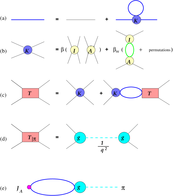
Figure 2:

Figure 3:

Figure 4:

Figure 5:

Figure 6:

References

- [1] F. Karsch, plenary talk at Lattice-93,Nucl. Phys. (Proc. Suppl.) B34 (1994) 63.
- [2] C. DeTar, plenary talk at Lattice-94,Nucl. Phys. (Proc. Suppl.)B. In press. Quark Gluon Plasma in numerical simulations of lattice QCD, to appear in ”Quark Gluon Plasma 2”, R. Hwa, ed., World Scientific (1995)
- [3] E. V. Shuryak, Nucl. Phys. B203, 93 (1982) 116.
- [4] D. I. Diakonov, V. Yu. Petrov Sov.Phys.Jetp 62 ( 1985) 204-214. (Zh. Eksp. Teor. Fiz. 89 ( 1985) 361-379). Nucl. Phys. B272 (1986) 457.
- [5] M. A. Nowak, J. J. M. Verbaarschot, I. Zahed Nucl. Phys. B324 (1989) 1.
- [6] E. Shuryak, Nucl. Phys. B302 (1988) 559, 574, 599, Nucl. Phys. B319 (1989) 521, 541.
- [7] E. V. Shuryak, J. J. M. Verbaarschot Nucl. Phys. B341 (1990) 1-26.
- [8] E. V. Shuryak, J. J. M. Verbaarschot Nucl. Phys. B410 (1993) 55-89. T. Schäfer, E. V. Shuryak, J. J. M. Verbaarschot Nucl. Phys. B412 (1994) 143; T. Schäfer, E. V. Shuryak, Phys. Rev. D50 (1994) 478.
- [9] T. Schäfer, E. V. Shuryak, Phys. Rev. Lett. 75 (1995) 1707.
- [10] T. Schäfer, E. V. Shuryak, Phys. Lett. B356 (1995) 147.
- [11] E. Shuryak, Rev. Mod. Phys. 65 (1993) 1.
- [12] M. C. Chu, J. M. Grandy, S. Huang and J. W. Negele, Phys. Rev. Lett. 70 (1993) 225; M. C. Chu and S. Huang, Phys. Rev. D45 (1992) 7.
- [13] M. C. Chu, J. M. Grandy, S. Huang, J. W. Negele, Phys. Rev. D49 (1994) 6039.
- [14] C. Michael, P. S. Spencer, Nucl. Phys. (Proc. Suppl.) B42 (1995) 261; Phys. Rev. D50 (1995) 7570.
- [15] E. Shuryak Phys.Lett. B79 (1978) 135.
- [16] R. D. Pisarski and L. G. Yaffe, Phys. Lett. B97 (1980) 110.
- [17] E. M. Ilgenfritz and E. Shuryak, Nucl. Phys. B319 (1989) 511.
- [18] E. Shuryak, M. Velkovsky Phys. Rev. D50 (1994) 3323-3327.
- [19] M. C. Chu, S. Schramm, Phys. Rev. D51 (1995) 4580.
- [20] E. M. Ilgenfritz, E. V. Shuryak Phys. Lett. B325 (1994) 263-266.
- [21] T. Schäfer, E. V. Shuryak, J. J. M. Verbaarschot Phys. Rev. D51 (1995) 1267.
- [22] E. V. Shuryak, J. J. M. Verbaarschot Nucl. Phys. B364 (1991) 255-282.
- [23] T. Schäfer, E. V. Shuryak, Interacting instanton liquid preprints, Stony Brook, SUNY-NTG-95-22,SUNY-NTG-95-23.
- [24] J. J. M. Verbaarschot Nucl. Phys. B362 (1991) 33.
- [25] Nucl. Phys. B245 (1984) 259.
- [26] C. Bernard Phys. Rev. D19 (1979) 3013.
- [27] Edward Shuryak Comments Nucl. Part. Phys. 21 (1994) 235-248.
- [28] G. ’t Hooft Phys. Rev. D14 (1976) 3432.
- [29] M. A. Nowak, J. J. M. Verbaarschot, I. Zahed Nucl. Phys. B325 (1989) 581.
- [30] D. J. Gross, R. D. Pisarski and L. G. Yaffe, Rev. Mod. Phys 53 (1981) 43.
- [31] S. Klimt, M. Lutz, U. Vogl and W. Weise Nucl. Phys. A516 (1990) 429-468.
- [32] U. Vogl and W. Weise Prog. Part. Nucl. Phys. 27 (1991) 195-272.
- [33] G. Boyd, S. Gupta, F. Karsch, E. Laermann Z. Phys. C64 (1994) 331.
- [34] E. Shuryak Comments Nucl. Part. Phys. 21 (1994) 235.
- [35] T. D. Cohen, Univ. of Maryland preprint no. 96-060.
- [36] S. Lee and T. Hatsuda, preprint hep-ph/9601373., Jan. 1996.
- [37] N. Evans,S. D. H. Hsu, M. Schwetz, preprint YCTP-P3-96, Jan. 1996.