HD-THEP-96-04 Nucleon Structure and High Energy Scattering

Abstract

If the pomeron is generated by a two gluon exchange there is no a priori reason for a drastic suppression of three gluon exchange with negative parity and charge parity. This would lead to an unacceptably large difference between $p\,p$ and $p\,\bar{p}$ scattering. It is shown that a natural suppression of the $C$=$P$=–1 contribution to high energy scattering is given by a cluster structure of the nucleon.

1 Introduction         The possibility that the real part of the scattering amplitude increases with energy as fast as the imaginary part was first considered by Lukaszuk and Nicolescu [1]. Such a behavior which is well compatible with our present knowledge of axiomatic field theory would mean that a trajectory of a pole which is odd under C and P has an intercept near one, it has been called odderon. One consequence of such an odderon would be that the ratio of the real to imaginary part of the forward scattering amplitude is different for particle particle and particle anti-particle scattering even at asymptotic energies. For further reference we shall use the conventional abbreviation $\Delta\rho$ for that difference:

$$\Delta\rho(s)=\rho^{\bar{p}p}(s)-\rho^{pp}(s)=\frac{{\rm Re}\left[T^{\bar{p}p}(s,0)\right]}{{\rm Im}\left[T^{\bar{p}p}(s,0)\right]}-\frac{{\rm Re}\left[T^{pp}(s,0)\right]}{{\rm Im}\left[T^{pp}(s,0)\right]}$$ (1)

Interest in the odderon rose again when the UA4 collaboration [2] reported a value for $\rho^{\bar{p}p}$ at $\sqrt{s}=546$ GeV which was much larger than the one extrapolated by means of dispersion relations for proton-proton scattering and a large value for$|\Delta\rho|$ seemed indicated.
The new results of the UA4/2 collaboration [3] obtained however a value $\rho^{\bar{p}p}(\sqrt{s}=541\makebox{ GeV})=0.135\pm 0.015$ which is very well compatible with $\Delta\rho=0$ at that energy (see e.g. [4]) and at any rate leaves no room for a large value of that quantity. The very successful description of high energy data by the Donnachie-Landshoff pomeron [5] yields also $\Delta\rho\approx 0$.
The new analysis of the $C$=$P$=–1 exchange had however shown that from the point of view of QCD the odderon was by no means an odd concept. In perturbative QCD it had been shown [6] that the exchange of three reggeized gluons leads in the leading log approximation of perturbative QCD to an intercept of the $C$=$P$=–1 trajectory above one, i.e. its contribution is increasing with energy (though slower than that of the perturbative pomeron). Similar results have also been obtained in a non-perturbative approach using the N/D method [7].
As far as the contribution of three non-perturbative gluons is concerned there is no reason for a strong suppression of the three gluon versus the two gluon exchange. In an Abelian model for non-perturbative gluon exchange [8] Donnachie and Landshoff [9] have found that the lowest order effective odderon coupling, i.e. the coupling of three non-perturbative gluons, is suppressed by a factor of two with respect to the effective pomeron coupling. Though it is very gratifying that in a non-perturbative model the three gluon coupling is smaller than the two gluon coupling (naive expectation goes in the opposite direction), this coupling still leads to a value of $|\Delta\rho|\approx.5$ which is far from consistent with the analysis of the data. In the Abelian model of Landshoff and Nachtmann, where quark additivity is a consequence of the model, the $\rho$-parameter for hadron-(anti)hadron scattering is just the one for quark-(anti)quark scattering.
In a series of papers ([10] and the literature quoted there) a non-Abelian model of high energy scattering was presented which gives a good description of the data and relates parameters of high energy scattering to those of hadron spectroscopy. One of the most characteristic features of this model is that the same mechanism which leads to confinement introduces a kind of string-string interaction in high energy scattering and leads to a marked increase of the total cross section as a function of the hadron size, even if the latter is large as compared to the gluonic correlation length. Quark additivity does not hold in that approach. The different total cross sections for pion-nucleon, kaon-nucleon and nucleon-(anti)nucleon scattering are correctly reproduced due to the different (electromagnetic) radii of the hadrons. In this note we evaluate the leading $C$=$P$=–1 contribution of that model. We show that this contribution (and therefore also $\Delta\rho$) depends crucially on the structure of the nucleon; we especially discuss the dependence of $\Delta\rho$ on the radius of a di-quark if two quarks are clustered.
Our paper is organized as follows: In section 2 we shortly refer to the main ingredients of the model of the stochastic vacuum (for a detailed description we refer to [10]) and calculate the $C$=$P$=–1 contribution to the scattering amplitude. In section 3 we give the numerical results for $\Delta\rho$ for different nucleon configurations and discuss the implications in section 4.

2 The color singlet $\bf C$=$\bf P$=–1 scattering amplitude
The main ingredients for the above mentioned treatment of non-perturbative high energy scattering are separation of the large energy from the small momentum transfer scale by the eikonal approximation for a fixed gluon vacuum field and subsequent averaging over these fields [11]; the averaging is done with the model of the stochastic vacuum (MSV) [12][13]. In our non-Abelian treatment it is crucial to respect gauge invariance and hence the fundamental processes are not quark-quark scattering, but rather ,,scattering” of Wegner-Wilson loops (see fig.(1)). For details we refer to [10] and only shortly indicate in words and figures the principal steps of the procedure.

As mentioned the principal ingredient is the scattering amplitude of two Wegner-Wilson loops with light-like sides. The line integrals $\exp\{-ig\int\mbox{\bf A}dz\}$ occuring along the light-like sides of the loops are just the eikonal phases of the constituents. In order to evaluate the amplitude, i.e. to perform the functional integration over the gluon fields, first the line integrals over the potentials are transformed into surface integrals over the field strengths by means of the non-Abelian Stokes theorem [14]. In doing so one has to introduce a reference point $C$ which is common to both the surfaces bordered by the loops (see fig.(2)). The expectation value of the two loops is then evaluated in the model of the stochastic vacuum which assumes that the non-perturbative gluonic contribution can be approximated by a Gaussian stochastic process in the field strengths $\mbox{\bf F}_{\mu\nu}$. This Gaussian process is characterized by the two-point function of two parallel transported field strengths expressed in the adjoint basis of the $SU(3)$

$$<F^{A}_{\mu\nu}(x,w)F^{B}_{\rho\sigma}(y,w)>.$$ (2)

Here $w$ is the coordinate of the reference point $C$ mentioned above (see fig.(2)). All higher correlators can be reduced to products of this two-point function for which the MSV makes a Lorentz- and gauge-invariant ansatz.

If we consider meson-meson scattering, the loops shown in fig.(1) must be averaged with a transversal meson wave function.
In order to describe baryon-baryon scattering, one has to start from three loops (without traces) with one common side as shown in fig.(3). From these loops a baryon is constructed by averaging with a transversal wave function. We consider two classes of configurations:
In the first case the distances from the common line of all three loops are equal and we vary the angle $\alpha$ between two loops (see fig.(3)). If this angle tends to zero the two quarks together form a point-like di-quark (i.e. an object transforming as the $\bar{3}$ representation of $SU(3)$).
The other case we consider is a linear structure of the nucleon.

The light-like components of the surface integrations of the Wegner-Wilson loops can be performed analytically and we end up in the transversal plane of the scattering process. In the following the transversal components of a vector are denoted by $\vec{x}=(0,x^{1},x^{2},0)$.
It is convenient to introduce a reduced scattering amplitude for baryon-baryon scattering [10] depending on the impact parameter $\vec{b}$ and the extension parameters $\vec{R}_{i}$ of the two baryons:

$$\tilde{J}(\vec{b},\vec{R}_{1},\vec{R}_{2}) = -<B_{1}\cdot B_{2}>$$

$${\rm with}\;B_{i} = \frac{1}{6}\epsilon_{abc}\epsilon_{a^{\prime}b^{\prime}c^{\prime}}\left\{W_{a^{\prime}a}[\mbox{$\cal S$}_{i1}]W_{b^{\prime}b}[\mbox{$\cal S$}_{i2}]W_{c^{\prime}c}[\mbox{$\cal S$}_{i3}]-\delta_{a^{\prime}a}\delta_{b^{\prime}b}\delta_{c^{\prime}c}\right\}.$$ (3)

The unitary $3\times 3$ matrices $\mbox{\bf W}[\mbox{$\cal S$}_{ij}]$ are the Wegner-Wilson loops

$$W_{a^{\prime}a}[\mbox{$\cal S$}_{ij}]=\left[\mbox{$\cal P$}\,e^{-ig\oint_{\partial S_{ij}}\mbox{\bf A}_{\mu}(z)\,{\rm d}z^{\mu}}\right]_{a^{\prime}a}$$ (4)

and the integration paths $\partial\mbox{$\cal S$}_{ij}$ are illustrated in fig.(3).
Before we proceed further we want to show that from this eq.(3) one can see easily that in the limit of the angle $\alpha$ (see fig.(3)) going to zero, the baryon can effectively treated like a meson; the resulting di-quark playing the role of the anti-quark. If $\alpha\rightarrow 0$ the loop $\partial\mbox{$\cal S$}_{i2}$ goes over into $\partial\mbox{$\cal S$}_{i1}$ and we have

$$B_{i}(\alpha=0)=\frac{1}{6}\epsilon_{abc}\epsilon_{a^{\prime}b^{\prime}c^{\prime}}\left\{W_{a^{\prime}a}[\mbox{$\cal S$}_{i1}]W_{b^{\prime}b}[\mbox{$\cal S$}_{i1}]W_{c^{\prime}c}[\mbox{$\cal S$}_{i3}]-\delta_{a^{\prime}a}\delta_{b^{\prime}b}\delta_{c^{\prime}c}\right\}.$$ (5)

We use the following identity for $SU(3)$ matrices

$$\epsilon_{a^{\prime}b^{\prime}c^{\prime}}W_{a^{\prime}a}W_{b^{\prime}b}W_{c^{\prime}c}=\epsilon_{abc}$$

from which we obtain

$$\epsilon_{a^{\prime}b^{\prime}c^{\prime}}W_{a^{\prime}a}[\mbox{$\cal S$}_{i1}]W_{b^{\prime}b}[\mbox{$\cal S$}_{i1}]=\epsilon_{abh}W^{-1}_{hc^{\prime}}[\mbox{$\cal S$}_{i1}]=\epsilon_{abh}W_{hc^{\prime}}[\mbox{$\cal S$}_{i1}^{-1}]$$ (6)

where $\partial\mbox{$\cal S$}_{i1}^{-1}$ is the Wegner-Wilson loop oriented in opposite direction. Inserting eq.(6) in eq.(5) we obtain

$$B_{i}(\alpha=0) = \frac{1}{3}\delta_{ab}\left\{W_{ac}[\mbox{$\cal S$}_{i1}^{-1}]W_{cb}[\mbox{$\cal S$}_{i3}]-\delta_{ab}\right\}=\frac{1}{3}\delta_{ab}\left\{W_{ab}[\hat{\mbox{$\cal S$}}_{i12}]-\delta_{ab}\right\}$$ (7)

$$= \frac{1}{3}\makebox{ Tr }\left\{\mbox{\bf W}[\hat{\mbox{$\cal S$}}_{i12}]-\mbox{\bf 1}\right\}$$

where $\partial\hat{\mbox{$\cal S$}}_{i12}$ is the union of $\partial\mbox{$\cal S$}_{i1}^{-1}$ and $\partial\mbox{$\cal S$}_{i3}$. This is exactly the contribution of a quark traveling along line 3 and an anti-quark traveling along line 1=2. The spin contribution in the high energy limit of a quark and anti-quark is equal, namely $2s\delta_{\lambda\lambda^{\prime}}$, where $\lambda$ is the helicity in the initial and final state respectively. Thus in the limit $\alpha\rightarrow 0$ the baryon can be treated effectively as a meson, the point like di-quark traveling along line 1=2 replacing the anti-quark of the meson.

After applying the non-Abelian Stokes theorem [14] the integration surface $S_{ij}$ of the Wegner-Wilson loop

$$W_{a^{\prime}a}[\mbox{$\cal S$}_{ij}]=\left[\mbox{$\cal P$}_{S}\,e^{-ig\frac{1}{2}\int_{S_{ij}}\mbox{\bf F}_{\mu\nu}(z,w)\,{\rm d}\sigma^{\mu\nu}(z)}\right]_{a^{\prime}a}$$ (8)

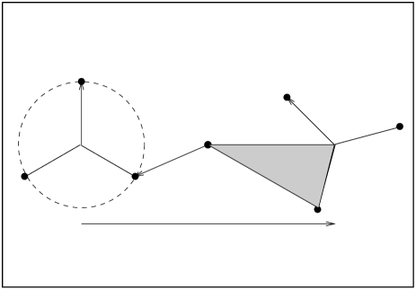
Figure 4: The geometry of the two baryons in the transversal plane. The vector pointing to quark $j$ of baryon $i$ ($q_{ij}$) is denoted by $\vec{r}_{ij}$ and the vector $\vec{R}_{i}$ points to quark $q_{i1}$. $S_{22}$ is the projection on the transversal plane of the integration surface for $W_{ee^{\prime}}[\mbox{$\cal S$}_{22}]$. In this picture the three quarks of a baryon are arranged like a star with equal angles, but the calculation is valid for any geometry.

are the sliding sides of the pyramid belonging to quark $j$ of baryon $i$ ($\mbox{$\cal P$}_{S}$ stands for surface-ordered integration). For an illustration in the transversal plane see fig.(4).

By averaging eq.(3) with wave functions with mean radius $S_{i}$,

$$\hat{J}(\vec{b}) = \int\,{\rm d^{2}}\vec{R}_{1}\int\,{\rm d^{2}}\vec{R}_{2}\,\tilde{J}(\vec{b},\vec{R}_{1},\vec{R}_{2})|\Psi(\vec{R}_{1})|^{2}|\Psi(\vec{R}_{2})|^{2}$$

$$\Psi(\vec{R}_{i}) = \sqrt{\frac{2}{\pi}}\frac{1}{S_{i}}e^{-\frac{|\vec{R}_{i}|^{2}}{S_{i}^{2}}},$$ (9)

the diffractive scattering amplitude $T$ at given center of mass energy $s$ is

$$T=2is\int\,{\rm d^{2}}\vec{b}\,\hat{J}(\vec{b},S_{1},S_{2}).$$

In order to calculate the scattering amplitude we first expand the exponential of the Wegner-Wilson loops (eq.(8)) in a power series and plug this into eq.(3). Then we express the parallel transported field strengths in the adjoint basis of the $SU(3)$ and perform the color-sums in eq.(3). Finally we apply factorization according the Gaussian model to the expectation value of the expanded field strengths (for a detailed discussion see again [10]) and perform the surface integration using the MSV-correlator. It has been shown that the surface integration over the correlator of a pair of field strengths coming from the same baryon vanishes and the color-sum is zero for only one field strength. So the leading contribution in the expansion of the Wegner-Wilson loops comes from four field strengths, two from baryon 1 and two from baryon 2. This contribution has been calculated in [10] and gives rise to a purely imaginary $C$=+1 scattering amplitude.
Now we calculate the next contribution where we have three field strengths from each baryon. There are three possibilities (see fig.(5)):
a) All three field strengths belong to the same quark.
b) Two field strengths come from the same quark and the third from another one.
c) To every quark belongs one field strength.

The color-sums for these three possibilities are:
a) (e.g. all three fields strengths come from $q_{13}$)

$$\epsilon_{abc}\epsilon_{abc^{\prime}}\left[\mbox{\bf t}^{C_{1}}\mbox{\bf t}^{C_{2}}\mbox{\bf t}^{C_{3}}\right]_{c^{\prime}c}=2\makebox{ Tr }\left[\mbox{\bf t}^{C_{1}}\mbox{\bf t}^{C_{2}}\mbox{\bf t}^{C_{3}}\right]=\frac{1}{2}d_{C_{1}C_{2}C_{3}}+\frac{i}{2}f_{C_{1}C_{2}C_{3}}$$ (10)

b) (e.g. two from $q_{13}$ and one from $q_{12}$)

$$\epsilon_{abc}\epsilon_{ab^{\prime}c^{\prime}}\,\mbox{\bf t}_{b^{\prime}b}^{B}\left[\mbox{\bf t}^{C_{1}}\mbox{\bf t}^{C_{2}}\right]_{c^{\prime}c}=-\frac{1}{4}d_{BC_{1}C_{2}}-\frac{i}{4}f_{BC_{1}C_{2}}$$ (11)

$$\mbox{c) }\epsilon_{abc}\epsilon_{a^{\prime}b^{\prime}c^{\prime}}\,\mbox{\bf t}_{a^{\prime}a}^{A}\,\mbox{\bf t}_{b^{\prime}b}^{B}\,\mbox{\bf t}_{c^{\prime}c}^{C}=\frac{1}{2}d_{ABC}$$ (12)

Here $f_{ABC}$ and $d_{ABC}$ are the structure constants and the symmetric $d$-symbols of $SU(3)$.
The next step is to factorize the expectation value into pairs. To avoid very long formulas we introduce the following shorthand notation:

$$\int\int<i^{A}j^{B}>\;:=\;\int_{S_{1i}}\int_{S_{2j}}<g^{2}\,F_{\mu\nu}^{A}(x,w)\,F_{\rho\sigma}^{B}(y,w)>\,{\rm d}\sigma^{\mu\nu}(x)\,{\rm d}\sigma^{\rho\sigma}(y)$$

For example $\int\int<2^{A}3^{B}>$ stands for the surface integration over the correlator with one field strength running over the pyramid belonging to quark 2 of baryon 1 and the other running over the pyramid belonging to quark 3 of baryon 2.
There are 7 permutations for coupling the two baryons depending on which possibility of a), b) or c) in fig.(5) is chosen.
Let us start with possibility a) for both baryons. Expanding e.g. $W_{c^{\prime}c}[\mbox{$\cal S$}_{13}]$ and $W_{f^{\prime}f}[\mbox{$\cal S$}_{23}]$ up to third order and using the color-sum eq.(10) we get the following contribution to eq.(3):

$$-\frac{1}{36}\left(\frac{-i}{2}\right)^{6}\left[\frac{1}{2}d_{C_{1}C_{2}C_{3}}+\frac{i}{2}f_{C_{1}C_{2}C_{3}}\right]\left[\frac{1}{2}d_{F_{1}F_{2}F_{3}}+\frac{i}{2}f_{F_{1}F_{2}F_{3}}\right]\times$$

$$\mbox{$\cal P$}_{S}\int\cdots\int<3^{C_{1}}3^{C_{2}}3^{C_{3}}\;3^{F_{1}}3^{F_{2}}3^{F_{3}}>$$ (13)

Now we factorize the expectation value into pairs. The $d_{C_{1}C_{2}C_{3}}\cdot f_{F_{1}F_{2}F_{3}}$ color structure vanishes because the correlator (eq.(2)) is diagonal in color. We thus arrive at the expression

$$\Rightarrow -\frac{1}{36\cdot 4}\left(\frac{-i}{2}\right)^{6}\left[d_{C_{1}C_{2}C_{3}}\cdot d_{F_{1}F_{2}F_{3}}-f_{C_{1}C_{2}C_{3}}\cdot f_{F_{1}F_{2}F_{3}}\right]\times$$ (14)

$$\mbox{$\cal P$}_{S}\int\cdots\int\left\{<3^{C_{1}}3^{F_{1}}><3^{C_{2}}3^{F_{2}}><3^{C_{3}}3^{F_{3}}>\,+\,\mbox{5 permutations}\right\}$$

The $d_{C_{1}C_{2}C_{3}}\cdot d_{F_{1}F_{2}F_{3}}$ color-sum is the same for all six factorizations whereas the $f_{C_{1}C_{2}C_{3}}\cdot f_{F_{1}F_{2}F_{3}}$ sum has different signs. In the first structure we can therefore replace the surface-ordered integrals by usual ones corrected with $1/3!$ for each baryon. Whereas in the second structure we have to perform the surface-ordered integrals what is technically very complicated. In this publication we concentrate on the $C=-1$ contribution and we will show that for this contribution only the $d\cdot d$ structure is needed.
If one baryon is replaced by an anti-baryon we have to invert the orientation of the corresponding Wegner-Wilson loops. This yields a factor $(-1)^{3}$. Furthermore inverting the surface ordering of the three field strengths gives an extra $(-1)$ for the $f$ structure whereas the $d$ structure is symmetric and remains unchanged. This shows that only the $d\cdot d$ structure gives rise to a change in sign by replacing one baryon by an anti-baryon.
We finally get, with $d_{C_{1}C_{2}C_{3}}\cdot d_{C_{1}C_{2}C_{3}}=\frac{40}{3}$,

$$\Rightarrow -\frac{1}{36\cdot 4}\left(\frac{-i}{2}\right)^{6}\frac{6}{3!\cdot 3!}\frac{40}{3}\frac{1}{(N_{C}^{2}-1)^{3}}\left[\int\int<3^{A}3^{A}>\right]^{3}$$ (15)

$$= -i\frac{5}{9\cdot 12^{3}\cdot(N_{C}^{2}-1)^{3}\cdot 36}\;\tilde{\chi}_{33}^{3}$$

where

$$\tilde{\chi}_{ij}:=\frac{-12i}{4}\int\int<i^{A}j^{A}>.$$

Taking into account all permutations for possibility a) we get:

$$-i\frac{5}{9\cdot 12^{3}\cdot(N_{C}^{2}-1)^{3}\cdot 36}\;\left[\tilde{\chi}_{11}^{3}+\tilde{\chi}_{12}^{3}+\tilde{\chi}_{13}^{3}+\tilde{\chi}_{21}^{3}+\tilde{\chi}_{22}^{3}+\tilde{\chi}_{23}^{3}+\tilde{\chi}_{31}^{3}+\tilde{\chi}_{32}^{3}+\tilde{\chi}_{33}^{3}\right]$$ (16)

The calculation of all the remaining contributions (all combinations of the three possibilities in fig.(5)) is very similar to the previous case so we only give the final result for the $C$=$P$=–1 contribution to the reduced scattering amplitude (eq.(3)):

$$\tilde{J}^{C=-1} = -i\frac{5}{9\cdot 12^{3}\cdot(N_{C}^{2}-1)^{3}\cdot 36}\times$$ (17)

$$\bigg{[}\tilde{\chi}_{11}^{3}\,+\,\mbox{8 per.}-\frac{3}{2}\tilde{\chi}_{11}^{2}\,\tilde{\chi}_{12}\,+\,\mbox{35 per.}$$

$$+\frac{3}{4}\tilde{\chi}_{11}^{2}\,\tilde{\chi}_{22}\,+\,\mbox{35 per.}\,+\,\frac{3}{2}\tilde{\chi}_{11}\,\tilde{\chi}_{12}\,\tilde{\chi}_{22}\,+\,\mbox{35 per.}+6\tilde{\chi}_{11}\,\tilde{\chi}_{12}\,\tilde{\chi}_{13}\,+\,\mbox{5 per.}$$

$$-3\tilde{\chi}_{11}\,\tilde{\chi}_{12}\,\tilde{\chi}_{23}\,+\,\mbox{35 per.}+6\tilde{\chi}_{11}\,\tilde{\chi}_{22}\,\tilde{\chi}_{33}\,+\,\mbox{5 per.}\bigg{]}.$$

The evaluation of the $\tilde{\chi}_{ij}$ follows the same lines as in reference [10].

3 Numerical results         Using eq.(17), eq.(9) and the results for ${\rm Im}\left[T^{pp}(s,0)\right]$ we compute the leading contribution to the rho parameter.

$$\Delta\rho(s)=\frac{{\rm Re}\left[T^{\bar{p}p}(s,0)\right]}{{\rm Im}\left[T^{\bar{p}p}(s,0)\right]}-\frac{{\rm Re}\left[T^{pp}(s,0)\right]}{{\rm Im}\left[T^{pp}(s,0)\right]}=-2\frac{{\rm Re}\left[T^{pp}(s,0)\right]}{{\rm Im}\left[T^{pp}(s,0)\right]}$$

The results depend on the geometry chosen for the baryon and on the parameters of the MSV, that is the correlation length $a$ and the condensate $<g^{2}FF>$. In the same way as it has been done in [10] the size of the proton, $a$ and $<g^{2}FF>$ have been determined in [15] for the star-like and a linear geometry (see fig.(6)). Here a somewhat more complete expression for the MSV-correlator (eq.(2)) has been used leading to a minor change of parameters as compared to [10]. At $\sqrt{s}=541$ GeV we found:

star-like linear $<g^{2}FF>$ 1.88 $\makebox{ GeV}^{4}$ 3.07 $\makebox{ GeV}^{4}$ $a$ 0.371 fm 0.332 fm $S_{\rm proton}$ 1.93 $a$ 2.62 $a$

Table 1: The two parameter sets

With this set of parameters we present in fig.(7) $\Delta\rho$ at $\sqrt{s}=541$ GeV as a function of $r_{\perp}$ and $r_{\|}$ (for illustration see fig.(6)).

4 Discussion         As can be seen from fig.(7) a clustering of two quarks to a di-quark with a radius smaller or equal to $0.3$ fm yields already a drastic suppression of $\Delta\rho$ to a value $|\Delta\rho|\leq 0.02$ which is compatible with the analysis of experiments.
It should be noted that even for a meson or baryon in the di-quark picture the contribution of the $C$=$P$=–1 exchange is appreciable for a given Wegner-Wilson loop. But constructing the hadrons by averaging the loops with wave functions cancels these contributions. For a clustering to a di-quark with finite radius the $C$=$P$=–1 contribution is suppressed but not completely canceled.
There is plenty of other evidence for di-quark clustering in baryons: The scaling violation in nucleon structure functions [16], the strong attraction in the scalar di-quark channel in the instanton vacuum [17] and the $\Delta I=\frac{1}{2}$ enhancement in semi leptonic decays of baryons [18]. Scaling violation in deep inelastic scattering is sensible to the form factors of the di-quark, which is modeled by a pole fit with a pole mass of $\sqrt{3}$ to $\sqrt{10}$ GeV. This corresponds to di-quark radii of 0.3 to 0.16 fm. They are according to our model sufficiently small to give a suppression of $\Delta\rho$ to values below 0.02 even for the transversal extension. If the nucleon has a linear structure no suppression by di-quark clustering is necessary at all.
Our calculation have been performed in a specific non-perturbative model. But since the limiting case of a vanishing di-quark radius leads quite generally to an odderon cancelation as in the case of mesons (see eq.(7) and the discussion of it) we think that the suppression of the $C$=$P$=–1 exchange is generally to be caused by the structure of the nucleon and cannot be seen on the quark level.

Acknowledgments         The authors thank G. Kulzinger, P. V. Landshoff and O. Nachtmann for discussions and valuable comments.

Figure 1: Two loops with transversal extension $\vec{R}_{1}$ and $\vec{R}_{2}$ and light-like sides. Loop 1 describes a colorless $q\bar{q}$-pair running in negative 3-direction and loop 2 in positive 3-direction. The impact parameter $\vec{b}$ is chosen to be purely transverse.

Figure 2: Somewhat tilted view of the loops after applying the non-Abelian Stoke’s theorem with the reference point $C$ which is common to both surfaces.

Figure 3: A baryon is constructed out of 3 loops with one common line which transforms like a color singlet. Here $\partial\mbox{$\cal S$}_{ij}$ denotes the loop corresponding to quark j of baryon i.

Figure 5: The three possibilities for arranging the three field strengths on the three quarks.

Figure 6: In this figure we show the two different geometries chosen for the baryon. The proton radius is given in table 1 and for small quark distances $r_{\perp}$ and $r_{\|}$ we have a di-quark configuration.

star-like geometry

( $a$=0.371 fm, $S$=1.93$a$ )

linear geometry

( $a$=0.332 fm, $S$=2.62$a$ )

Figure 7: $\Delta\rho$ at UA4/2 energies for proton-(anti)proton scattering as a function of the quark distances $r_{\perp}$ and $r_{\|}$. Note the different scales.

References

• [1] L. Lukaszuk, B. Nicolescu, Lett.Nuov.Cim.8 (1973) 405
• [2] UA4 Collaboration (D. Bernard et.al. ), Phys.Lett.B198 (1987) 583
• [3] UA4/2 Collaboration (D. Bernard et.al. ), Phys.Lett.B316 (1993) 448
• [4] C. Bourelly, A. Martin, Proc. of the LHC workshop, Lausanne (1984)
A. Donnachie, P. Landshoff, Nucl.Phys.B244 (1984) 322
C. Bourelly, J. Soffer, T. T. Wu, Phys.Lett.B196 (1987) 237
P. Gauron, E. Leader, B. Nicolescu, Nucl.Phys.B299 (1988) 640
P. Kroll, W. Schweiger, Nucl.Phys.A503 (1989) 865
R. J. M. Covolan et al., Z.Phys.C58 (1993) 109
• [5] A. Donnachie, P. V. Landshoff, Phys.Lett.B296 (1992) 227
• [6] P. Gauron, Proc. V.th Blois workshop, ed. Fried et al. Singapore 1994
• [7] A. P. Contogouris, V.th Blois workshop, ed. Fried et al. Singapore 1994
• [8] P. V. Landshoff, O. Nachtmann, Z.Phys.C35 (1987) 405
• [9] A. Donnachie, P. V. Landshoff, Nucl.Phys.B348 (1991) 297
• [10] H. G. Dosch, E. Ferreira, A. Krämer, Phys.Rev.D50 (1994) 1992
• [11] O. Nachtmann, Ann.Phys.209 (1991) 436
• [12] H .G. Dosch, Phys.Lett.B190 (1987) 177
• [13] H. G. Dosch, Y. A. Simonov, Phys.Lett.B205 (1988) 339
• [14] N. E. Bralic, Phys.Rev.D22 (1980) 3090
Y. A. Simonov, Sov.J.Nucl.Phys.50 (1989) 134
• [15] H. G. Dosch, E. Ferreira, G. Kulzinger, M. Rueter, in preparation
• [16] M. Anselmino, E. Predazzi, S. Ekelin, D. B. Lichtenberg, Rev.Mod.Phys.65 (1993) 1199
• [17] T. Schäfer, E. V. Shuryak, J. J. M. Verbaarschot, Nucl.Phys.B142 (1994) 143
• [18] H. G. Dosch, M. Jamin, B. Stech, Z.Phys.C42 (1989) 167
Refer to caption
loop 1loop 2$\vec{x}$ $x^{0}$ $x^{3}$ $\vec{R}_{1}$ $\vec{R}_{2}$ $\vec{b}$