IASSNS-HEP-96/20
hep-ph/9603212
February 1996

Leptophobic $U(1)$’s and the $R_{b}$–$R_{c}$ Crisis
K.S. Babu, Chris Kolda, and John March-Russell

School of Natural Sciences,
Institute for Advanced Study,
Princeton, NJ 08540

In this paper, we investigate the possibility of explaining both the $R_{b}$ excess and the $R_{c}$ deficit reported by the LEP experiments through $Z$-$Z^{\prime}$ mixing effects. We have constructed a set of models consistent with a restrictive set of principles: unification of the Standard Model (SM) gauge couplings, vector-like additional matter, and couplings which are both generation-independent and leptophobic. These models are anomaly-free, perturbative up to the GUT scale, and contain realistic mass spectra. Out of this class of models, we find three explicit realizations which fit the LEP data to a far better extent than the unmodified SM or MSSM and satisfy all other phenomenological constraints which we have investigated. One realization, the $\eta$-model coming from $E_{6}$, is particularly attractive, arising naturally from geometrical compactifications of heterotic string theory. This conclusion depends crucially on the inclusion of a $U(1)$ kinetic mixing term, whose value is correctly predicted by renormalization group running in the $E_{6}$ model given one discrete choice of spectra.

1 Introduction & Principles

During the past six years the four experiments at LEP have provided an abundance of data supporting the Standard Model (SM) of particle physics and its $SU(3)_{c}\times SU(2)_{L}\times U(1)_{Y}$ gauge group structure. Until recently there has been no significant deviation pointing to new sources of physics beyond the SM. However, within the last two years there has been growing evidence that a discrepancy exists between the predicted and measured widths for the $b$ and $c$-quark decays of the $Z$ boson. In particular, LEP has reported measurements of [1]:

$$\left.\begin{array}[]{c}R_{b}\\ R_{c}\end{array}\right\}\equiv\frac{\Gamma(Z\to\overline{b}b/\overline{c}c)}{\Gamma(Z\to{\rm hadrons})}=\left\{\begin{array}[]{c}0.2219\pm 0.0017\\ 0.1543\pm 0.0074\end{array}\right.$$ (1)

These values differ from the SM predictions, $R_{b}=0.2152\pm 0.0005$ and $R_{c}=0.1714\pm 0.0001$ [2] (for $m_{t}=(176\pm 13)\,{\rm GeV}$[3] and $\alpha_{s}=0.125\pm 0.010$), by $3.9\sigma$ and $-2.3\sigma$ respectively.

If one is willing to accept the $R_{c}$ discrepancy as statistical, then there are many new sources of physics which can serve to resolve the $R_{b}$ measurement by only changing the couplings of the third-generation fermions. Such a method is naturally provided by low-energy supersymmetry (SUSY) with light charginos and stops [4], or by additional fermions mixing with, or additional interactions of, the $b$ and $t$ quarks [5]. However, if one interprets the $R_{c}$ deficit as another signal of new physics, then the scenarios for new physics are more limited [6].

A potential hurdle which one must face with respect to simultaneously explaining the $R_{b}$ excess and the $R_{c}$ deficit is that the LEP measurement for the total hadronic width of the $Z$ is in good agreement with the SM prediction ($\Gamma_{\rm had}=(1744.8\pm 3.0)\,{\rm MeV}$ at LEP versus $\Gamma_{\rm had}=(1743.5\pm 3.1)\,{\rm MeV}$ in the SM), while the sum $R_{b}+R_{c}$ is in slight disagreement with the SM prediction. That is, $R_{b}+R_{c}=0.3762\pm 0.0070$ as measured at LEP (with the error correlations properly included), versus a theoretical expectation of $0.3866\pm 0.0005$, $1.5\sigma$ apart.

A clue to solving this conundrum may lie in a simple observation. Defining $\Delta\Gamma_{i}$ as the difference between the experimental and the theoretical determinations of $\Gamma_{i}$, one notes that

$$3\Delta\Gamma_{b}+2\Delta\Gamma_{c}=(-23.2\pm 24.3)\,{\rm MeV}$$ (2)

so that at the $1\sigma$ level, a consistent interpretation of the data is given by assuming a flavor-dependent but generation-independent shift in the hadronic $Z$-couplings. That is,

$$\Gamma_{u,c} = \Gamma^{\rm SM}_{u,c}+\Delta\Gamma_{c}$$

$$\Gamma_{d,s,b} = \Gamma^{\rm SM}_{d,s,b}+\Delta\Gamma_{b}.$$ (3)

Such a pattern of shifts has also been suggested in [7, 8, 9].

A second hurdle in explaining the $R_{b}$ and $R_{c}$ puzzles is that unlike the partial hadronic widths of the $Z$, the well-measured partial leptonic widths are in good agreement with the SM predictions: $\Gamma_{e}=83.93\pm 0.14\,{\rm MeV}$ and $\Gamma_{\rm inv}=499.9\pm 2.5\,{\rm MeV}$, which are within $0.4\sigma$ and $-0.4\sigma$ respectively of theory. Any source of new physics must preserve the successful predictions of the SM for the leptonic widths.

In this paper we propose to explain the $R_{b}-R_{c}$ problem by introducing an additional $U(1)^{\prime}$ gauge symmetry. If this new $U(1)^{\prime}$ is broken near the electroweak scale, there can be significant mixing between the usual $Z$ and the new $Z^{\prime}$. The physical $Z$-boson as produced at LEP will then have its couplings to fermions altered by an amount proportional to the $Z-Z^{\prime}$ mixing angle times the $Z^{\prime}$ coupling to those same fermions.

Analyses have recently appeared in the literature [8, 9] that seek to fit the LEP data by introducing such an additional $U(1)^{\prime}$. Both of these works make a phenomenological fit to the data introducing some number of new parameters, such as arbitrary $U(1)^{\prime}$ charge ratios, $Z-Z^{\prime}$ mixing angle, and $Z^{\prime}$ mass. These analyses do indicate that this class of scenarios has the potential to solve the $R_{b}-R_{c}$ discrepancy, and are therefore interesting. However, they share some fundamental problems associated with the lack of an underlying, consistent framework. For example, the extra $U(1)^{\prime}$ is not anomaly free (this is true both for the $[U(1)^{\prime}]^{3}$, and most seriously, the mixed SM-$U(1)^{\prime}$ anomalies). Further, since the authors of [8, 9] also seek to explain the CDF dijet excess, they are forced to take a high value of the $Z^{\prime}$ mass. For such $Z^{\prime}$ masses, the $U(1)^{\prime}$-couplings have to be so large that the $U(1)^{\prime}$ gauge coupling becomes non-perturbative at most a decade above the $Z^{\prime}$ mass scale; implicit in this is that the $Z^{\prime}$ width in these models equals or even exceeds the $Z^{\prime}$ mass.

Here we will take a different approach. We set forth a few basic principles which we believe any attractive $Z^{\prime}$-model should obey. Within this framework we will find that there exist only limited classes of $U(1)^{\prime}$ models which are phenomenologically viable and theoretically consistent. Each class has a well-defined prediction for the $U(1)^{\prime}$ charges of the SM fermions, reducing much of the arbitrariness in the couplings. We will not attempt to explain the CDF dijet anomaly.

The principles that we demand are:

• The low energy spectrum must be consistent with the unification of the standard model gauge couplings that occurs in the minimal supersymmetric standard model (MSSM). This will lead us to consider models which are extensions of the MSSM, with any non-MSSM matter added in particular combinations which can be thought of as filling complete multiplets of $SU(5)$. We allow the possibility of unification within a string framework, and do not require the presence of a field theoretic GUT.

• All non-MSSM matter must fall into vector-like representations under the SM gauge groups. Such a requirement is consistent with the absence of experimental evidence for new fermions with masses below the top quark mass. Further, note that additional chiral matter is disfavored by the electroweak precision measurements, since, in contrast to vector-like matter it can give very large contributions to the $S$, $T$, and $U$ parameters.

• The $U(1)^{\prime}$ charges of the SM leptons must be (to a good approximation) zero. This requirement of leptophobia is motivated by the phenomenology. This alone will eliminate the $U(1)$ factors associated with most traditional GUT groups, since GUT’s tend to place leptons and quarks into common multiplets.

• Consistent with Eq. (3), we require that the $U(1)^{\prime}$ couplings be generation-independent. This requirement is essential if tree–level hadronic flavor changing neutral current processes mediated by the $U(1)^{\prime}$ gauge boson are to be naturally suppressed. This also has the advantage of simplicity and economy.

To be precise, the principle of unification that we will impose requires that the meeting of the SM couplings at $2\times 10^{16}~{}\,{\rm GeV}$ is not a coincidence. For simplicity we will not explicitly consider in this article the various string models where the scale of unification is increased to the (weak-coupling prediction of the) string unification scale $M_{\rm str}^{\rm 1-loop}\sim 5\times 10^{17}~{}\,{\rm GeV}$, such as those discussed in [10], although it will be clear that the consequences for our discussion of such a modification are slight. (Note that one interesting possibility that could maintain unification at $2\times 10^{16}~{}\,{\rm GeV}$ is the strongly coupled string scenario recently proposed by Witten [11].)

If one takes the unification of gauge couplings to imply the existence of a simple GUT gauge group, then the natural candidates with extra $U(1)$’s and three chiral families are $SO(10)$ and $E_{6}$. However the single additional $U(1)$ within $SO(10)$ is not leptophobic. In $E_{6}$ all linear combinations of the two additional $U(1)$’s orthogonal to hypercharge couple to leptons. Nonetheless, we will show that by including an effect usually overlooked in the literature ($U(1)$-mixing in the kinetic terms through renormalization group flow [12, 13]) there exists a unique $U(1)^{\prime}$ in the $E_{6}$ group which is compatible with the data. The $E_{6}$ subgroup in question is usually known in the literature as the $\eta$-model and interestingly is the unique model which results from $E_{6}$ Wilson–line breaking directly to a rank-5 subgroup in a string context [14]. We will discuss this case in some detail in Section 4.

Finally, although we assume the MSSM for the purposes of gauge coupling unification, we do not use MSSM loop contributions to the $Z\overline{b}b$ vertex in order to explain any part of the $R_{b}$ anomaly. In particular we do not assume light charginos or top squarks which are the necessary ingredients for such a scenario [4].

2 $Z-Z^{\prime}$ Mixing

We begin with a brief general discussion of $Z-Z^{\prime}$ mixing in the context of an $SU(2)_{L}\times U(1)_{Y}\times U(1)^{\prime}$ model. A more detailed discussion can be found, for example, in Refs. [15, 16]. The neutral current Lagrangian of the $Z$ and $Z^{\prime}$ is given by

$${\cal L}_{\rm NC}=\frac{1}{2}\sum_{i}\overline{\psi}_{i}\gamma^{\mu}\left(\frac{g_{2}}{c_{W}}(v_{i}+a_{i}\gamma^{5})Z_{\mu}+g^{\prime}(v^{\prime}_{i}+a^{\prime}_{i}\gamma^{5})Z^{\prime}_{\mu}\right)\psi_{i}$$ (4)

where

$$v_{i}=T_{3i}-2Q_{i}s^{2}_{W},\quad\quad\quad\quad a_{i}=-T_{3i}$$ (5)

are the SM vector and axial couplings of the $Z$, and $v^{\prime}$, $a^{\prime}$ are the (unknown) vector and axial couplings of the $Z^{\prime}$. Here $g^{\prime}$ is the coupling constant of the new $U(1)^{\prime}$ and $s^{2}_{W}\equiv\sin^{2}\theta_{W}$.

After electroweak and $U(1)^{\prime}$ breaking, the $Z$ and $Z^{\prime}$ gauge bosons mix to form the mass eigenstates $Z_{1,2}$, where we will identify the $Z_{1}$ with the gauge boson produced at LEP:

$$Z_{1} = \cos\xi\,Z+\sin\xi\,Z^{\prime}$$

$$Z_{2} = -\sin\xi\,Z+\cos\xi\,Z^{\prime}.$$ (6)

Since such mixing must necessarily be small in order to explain the general agreement between LEP results and the SM, we will throughout this paper use the approximation $Z_{1}\simeq Z+\xi Z^{\prime}$. We will also assume that the mass of the $Z_{2}$ is large enough so that its effects at LEP, either via direct production or loop effects can be ignored. Therefore all new physics effects must appear through the mixing angle $\xi$. The relevant Lagrangian probed at LEP will then be

$${\cal L}_{Z_{1}}=\frac{g_{2}}{2c_{W}}\sum_{i}\overline{\psi}_{i}\gamma^{\mu}(\overline{v}_{i}+\overline{a}_{i}\gamma^{5})Z_{1\mu}\psi_{i}$$ (7)

where, for small $\xi$,

$$\overline{v}_{i} \simeq v_{i}+\overline{\xi}v^{\prime}_{i}$$

$$\overline{a}_{i} \simeq a_{i}+\overline{\xi}a^{\prime}_{i},$$ (8)

and we have defined the auxiliary quantity

$$\overline{\xi}\equiv(g^{\prime}c_{W}/g_{2})\,\xi.$$ (9)

Because the $Z_{1}$ is no longer purely the electroweak $Z$, the $\rho$-parameter

$$\rho-1\equiv 4\sqrt{2}\,G_{F}\left(\Pi_{11}(0)-\Pi_{33}(0)\right)$$ (10)

receives a tree-level correction. (Here $\Pi_{ii}(0)$ are the $SU(2)_{L}$ vacuum polarization amplitudes at zero momentum transfer.) If we define the corrections to $\rho$ by

$$\rho\equiv 1+\Delta\rho_{SM}+\Delta{\overline{\rho}},$$ (11)

where $\Delta\rho_{SM}$ is due to loop corrections already present in the SM (such as the top), then the mixing with the $Z^{\prime}$ contributes to $\Delta{\overline{\rho}}$. Since we will later be interested in taking into account the effects of further shifts in $\rho$ due to the rest of the MSSM spectrum, we decompose $\Delta{\overline{\rho}}=\Delta\rho_{\rm M}+\Delta\rho_{\rm extra}$, where $\Delta\rho_{\rm M}$ is the part due to mixing with the $Z^{\prime}$. The value of $\Delta{\overline{\rho}}$ is the quantity that our fits to the LEP data will directly constrain. Writing the $Z-Z^{\prime}$ mass matrix as

$$M^{2}_{Z,Z^{\prime}}=\left(\begin{array}[]{cc}m^{2}_{Z}&\Delta m^{2}\\ \Delta m^{2}&M^{2}_{Z^{\prime}}\end{array}\right),$$ (12)

then for $M^{2}_{Z^{\prime}}\gg m^{2}_{Z}$, $\Delta m^{2}$, one finds that the shift in $\rho$ due to mixing, $\Delta\rho_{M}$, is given by

$$\Delta\rho_{M}\simeq\xi^{2}\left(\frac{m^{2}_{Z_{2}}}{m^{2}_{Z_{1}}}\right)\simeq\xi^{2}\left(\frac{M^{2}_{Z^{\prime}}}{m^{2}_{Z}}\right),$$ (13)

where

$$\xi\simeq-{\Delta m^{2}\over M_{Z^{\prime}}^{2}}.$$ (14)

There is also a corresponding shift in $s^{2}_{W}$:

$$s^{2}_{W}=s^{2}_{W}|_{\xi=0}-\frac{s_{W}^{2}c_{W}^{2}}{c_{W}^{2}-s_{W}^{2}}{\Delta\rho_{M}}.$$ (15)

In terms of the above parameters, one can then calculate the $Z_{1}$ partial width to fermions:

$$\Gamma(Z_{1}\to\overline{f}f)=\frac{G_{F}\,m^{3}_{Z_{1}}}{6\sqrt{2}\,\pi}\rho N_{c}\left(\overline{v}_{f}^{2}+\overline{a}_{f}^{2}\right).$$ (16)

A further relation may be obtained by examining the specific form of the terms that come into Eq. (12). If we assume that the fields $\phi_{i}$ which receive vev’s occur only in doublets or singlets of $SU(2)_{L}$, then

$$m^{2}_{Z} = \frac{2g^{2}_{2}}{c^{2}_{W}}\sum_{i}\langle T_{3i}\phi_{i}\rangle^{2}\quad=\quad\frac{g^{2}_{2}}{2c^{2}_{W}}v^{2}_{Z},$$

$$M^{2}_{Z^{\prime}} = 2g^{\prime 2}\sum_{i}\langle Q^{\prime}_{i}\phi_{i}\rangle^{2},$$ (17)

$$\Delta m^{2} = \frac{2g_{2}g^{\prime}}{c_{W}}\sum_{i}\langle T_{3i}\phi_{i}\rangle\langle Q^{\prime}_{i}\phi_{i}\rangle,$$

where $Q^{\prime}_{i}$ is the $U(1)^{\prime}$ charge of $\phi_{i}$ and $v^{2}_{Z}$ is the sum of the vev’s of the $SU(2)_{L}$ doublets. Then we may write $\Delta\rho_{M}$ as a simple function of $\overline{\xi}$:

$$\Delta\rho_{M}\simeq-\left(\frac{g_{2}}{g^{\prime}c_{W}}\right)\left(\frac{\Delta m^{2}}{m^{2}_{Z}}\right)\overline{\xi}=-{4\overline{\xi}\over v^{2}_{Z}}\sum_{i}\langle T_{3i}\phi_{i}\rangle\langle Q^{\prime}_{i}\phi_{i}\rangle.$$ (18)

What is noteworthy about this relationship is that it is connects the two quantities ($\Delta\rho_{M}$ and $\overline{\xi}$) which are experimentally constrained at LEP (up to $\Delta\rho_{\rm extra}$, which we can bound), in a way that is independent of the unknown gauge coupling $g^{\prime}$ and the $Z^{\prime}$ mass. Note that $\Delta m^{2}$ and $\overline{\xi}$ in Eq. (18) have opposite signs, so that $\Delta\rho_{M}$ is always positive.

2.1 $U(1)_{a}\times U(1)_{b}$ Mixing and RGE’s

The discussion so far has echoed the conventional wisdom on the subject of $Z-Z^{\prime}$ mixing. However, it was realized many years ago [12] that in a theory with two $U(1)$ factors, there can appear in the Lagrangian a term consistent with all gauge symmetries which mixes the two $U(1)$’s. In the basis in which the interaction terms have the canonical form, the pure gauge part of the Lagrangian for an arbitrary $U(1)_{a}\times U(1)_{b}$ theory can be written

$${\cal L} = -\frac{1}{4}\,F_{(a)}^{\mu\nu}F_{(a)\mu\nu}-\frac{1}{4}\,F_{(b)}^{\mu\nu}F_{(b)\mu\nu}-\frac{\sin\chi}{2}\,F_{(a)}^{\mu\nu}F_{(b)\mu\nu}$$ (19)

$$+~{}\Delta m^{2}A_{(a)\mu}A_{(b)}^{\mu}+\frac{1}{2}m_{a}^{2}A_{(a)\mu}A_{(a)}^{\mu}+\frac{1}{2}m_{b}^{2}A_{(b)\mu}A_{(b)}^{\mu}$$

If both $U(1)$’s arise from the breaking of some simple group $G\to U(1)_{a}\times U(1)_{b}$, then sin$\chi=0$ at tree level. However, if the matter of the effective low-energy supersymmetric theory is such that

$$\sum_{i={\rm chiral~{}fields}}\left(Q_{a}^{i}Q_{b}^{i}\right)\neq 0,$$ (20)

then non-zero $\chi$ will be generated at one-loop. This is naturally the case when split multiplets of the original non-Abelian gauge symmetry, such as the Higgs doublets in a grand unified theory, are present in the effective theory. Since we are interested in a large separation of scales, $M_{GUT}$ and $M_{Z}$, we will need to resum the large logarithms that appear [13, 17] using the renormalization group equations (RGE’s) for the evolution of the gauge couplings including the off-diagonal terms.

Once a non-zero $\chi$ (or $\Delta m^{2}$) has been induced, one needs to transform to the mass eigenstate basis. To do so, one must perform a (non-unitary) transformation on the original gauge fields, $A_{(a)}$ and $A_{(b)}$, to arrive at the mass eigenstates, $Z_{1,2}$:

$$A_{(a)} = \left(\cos\xi-\tan\chi\sin\xi\right)Z_{1}-\left(\sin\xi+\tan\chi\cos\xi\right)Z_{2}$$

$$A_{(b)} = \left(\sin\xi\,Z_{1}+\cos\xi\,Z_{2}\right)/\cos\chi,$$ (21)

where

$$\tan 2\xi=\frac{-2\cos\chi\,(\Delta m^{2}-m_{a}^{2}\sin\chi)}{m_{b}^{2}-m_{a}^{2}\cos 2\chi+2\,\Delta m^{2}\sin\chi}.$$ (22)

This transformation results in a shift in the effective charge to which one of the original $U(1)$’s couples. (One $U(1)$ can always be chosen to have unshifted charges.) This can be seen by taking the $\xi=0$ limit of the above transformation. The resulting interaction Lagragian is then of the form [12]:

$${\cal L}_{\rm int}=\overline{\psi}\,\gamma^{\mu}\left(g_{a}Q_{a}Z_{1\mu}+(g_{b}Q_{b}+g_{ab}Q_{a})Z_{2\mu}\right)\psi$$ (23)

where the redefined gauge couplings are related to the original couplings, $g^{0}$, by $g_{a}=g_{a}^{0}$, $g_{b}=g_{b}^{0}/\cos\chi$ and $g_{ab}=-g_{a}^{0}\tan\chi$. The ratio $\delta\equiv g_{ab}/g_{b}$ is a phenomenologically useful parameter, representing the shift in the $Z_{2}$–fermion coupling due to kinetic mixing.

The renormalization group equations for the coupling–constant flow of a $U(1)_{a}\times U(1)_{b}$ theory, including the off–diagonal mixing, are most usefully formulated in the basis of Eq. (23). In this basis the equations for the couplings $g_{a},g_{b}$ and $g_{ab}$ are:

$${dg_{a}\over dt} = \frac{1}{16\pi^{2}}g_{a}^{3}B_{aa},$$

$${dg_{b}\over dt} = \frac{1}{16\pi^{2}}g_{b}\biggl{(}g_{b}^{2}B_{bb}+g_{ab}^{2}B_{aa}+2g_{b}g_{ab}B_{ab}\biggr{)},$$ (24)

$${dg_{ab}\over dt} = \frac{1}{16\pi^{2}}\biggl{(}g_{b}^{2}g_{ab}B_{bb}+g_{ab}^{3}B_{aa}+2g_{a}^{2}g_{ab}B_{aa}+2g_{a}^{2}g_{b}B_{ab}+2g_{b}g_{ab}^{2}B_{ab}\biggr{)},$$

where $B_{ij}=\mathop{\rm tr}(Q_{i}Q_{j})$ with the trace taken over all the chiral superfields in the effective theory, and there is no sum over $(a,b)$ in Eq. (24). From these equations we immediately see that even if $g_{ab}=0$ to begin with, a non-zero value of the off-diagonal coupling is generated if the inner–product $\mathop{\rm tr}(Q_{i}Q_{j})$ between the two charges is non–zero. The advantage of this basis for the RGE’s is that the low-energy value of the parameter $\delta$ is given directly by the ratio $g_{ab}/g_{b}$ evaluated at the low scale. (This is not the case for the more symmetrical form of the RGE’s given in Ref. [13].)

For the case at hand, we will choose the couplings of the usual $Z_{\mu}$ to be canonical, shifting the charge of the $Z^{\prime}_{\mu}$. Since it is the $B_{\mu}$ component of $Z_{\mu}$ which mixes through the kinetic terms, the couplings of the $Z^{\prime}$ to matter fields can be expressed in terms of an effective $U(1)^{\prime}$ charge $Q_{\rm eff}=Q^{\prime}+Y\delta$, where $Y$ is hypercharge. We can translate from Eq. (23) using $g_{a}=g_{2}/c_{W}$ and $g_{b}=g^{\prime}$ so that $g_{ab}=-g_{2}\tan\theta_{W}\tan\chi$ and $\delta=g_{ab}/g_{b}$. The vector and axial couplings that come into Eq. (8) are given by

$$v^{\prime} = Q_{\rm eff}(\psi)-Q_{\rm eff}(\psi^{c})$$

$$a^{\prime} = -Q_{\rm eff}(\psi)-Q_{\rm eff}(\psi^{c}).$$ (25)

Note that both $\psi$ and $\psi^{c}$ are left-handed chiral fields: $Q_{\rm eff}(\psi^{c})=-Q_{\rm eff}(\psi_{R})$.

In most of the models we will consider, we will work directly with $Q_{\rm eff}$; in such models, whether or not $Q_{\rm eff}$ can be expressed as some $Q^{\prime}+Y\delta$ for non–zero $\delta$ will not have an effect on the analysis. However, when considering the $\eta$–model coming from $E_{6}$, the difference between $Q_{\rm eff}$ and $Q_{\eta}$ will have important consequences on the observable physics. We reserve further comment on the $U(1)$ mixing in the $E_{6}$ model until Section 4.

Kinetic mixing of $U(1)$’s will also shift the $\rho$-parameter. In the previous subsection we had assumed that we could write the electroweak $Z$ in terms of the mass eigenstates as $Z=\cos\xi\,Z_{1}-\sin\xi\,Z_{2}$. However, in the presence of a non–zero $\chi$ (or $\delta$), this is changed to (see Eq. (21), replacing $\tan\chi$ with $-s_{W}\tan\chi$):

$$Z = (\cos\xi+\sin\xi s_{W}\tan\chi)\,Z_{1}-(\sin\xi-\cos\xi s_{W}\tan\chi)\,Z_{2}$$

$$Z^{\prime} = (\sin\xi\,Z_{1}+\cos\xi\,Z_{2})/\cos\chi$$ (26)

$$A = \gamma-c_{W}\tan\chi(\sin\xi\,Z_{1}+\cos\xi\,Z_{2})$$

where $\gamma$ is the physical photon. Eq. (22) for $\xi$ becomes

$$\tan 2\xi=\frac{-2\cos\chi(\Delta m^{2}+m_{Z}^{2}s_{W}\sin\chi)}{M^{2}_{Z^{\prime}}-m_{Z}^{2}\cos^{2}\chi+m_{Z}^{2}s^{2}_{W}\sin^{2}\chi-2\,\Delta m^{2}s_{W}\sin\chi},$$ (27)

while the $Z_{1}$ mass is given to lowest order in $m_{Z}^{2}/M_{Z^{\prime}}^{2}$ by:

$$m_{Z_{1}}^{2}=m_{Z}^{2}\left\{1-\frac{m_{Z}^{2}}{M_{Z^{\prime}}^{2}}\left(\frac{\Delta m^{2}}{m_{Z}^{2}}+s_{W}\sin\chi\right)^{2}\right\}.$$ (28)

The coefficient of the $Z_{1}$ term in Eq. (26) is essentially a wave-function renormalization for the $Z_{1}$ and contributes to $\Delta\rho_{M}$ by absorbing part of the explicit mass shift which came from mass matrix mixing [16]. The net effect is a negative contribution to $\Delta\rho_{M}$ which subtracts from the positive definite contribution coming from mass mixing. In terms of $\delta$,

$$\Delta\rho_{M}\simeq\frac{M^{2}_{Z^{\prime}}}{m_{Z}^{2}}\xi^{2}-2k\xi\delta$$ (29)

where $k=g^{\prime}c_{W}s_{W}/g_{2}$. The important point to note is that, in the presence of kinetic mixing, $\Delta\rho_{M}$ can be smaller than had there been no such mixing; in fact, $\Delta\rho_{M}$ can be negative.

The kinetic mixing also shifts $s^{2}_{W}$ beyond what was already included in Eq. (15):

$$s^{2}_{W}=s^{2}_{W}|_{\xi=\delta=0}-\xi c_{W}^{2}\left(\frac{s_{W}^{2}}{c_{W}^{2}-s_{W}^{2}}\frac{M^{2}_{Z^{\prime}}}{m_{Z}^{2}}\xi+k\delta\right).$$ (30)

For $\delta=0$ this reduces to Eq. (15). Finally, there is a new contribution, $S_{M}$, to the so-called $S$-parameter (see, e.g., Ref. [16]) due to kinetic mixing which can be negative:

$$\alpha S_{M}\simeq-4c^{2}_{W}k\xi\delta$$ (31)

to leading order in $m_{Z}^{2}/M_{Z^{\prime}}^{2}$.

2.2 New Contributions to Oblique Parameters

As noted in the previous Sections, in the absence of $U(1)$ kinetic mixing (i.e., $\delta=0$), $Z$–$Z^{\prime}$ mixing gives a positive contribution to the $\rho$–parameter, denoted by $\Delta\rho_{M}$, and no contribution to the $S$-parameter. Since our numerical fits are sensitive to the total $\Delta\overline{\rho}$ and $S$, it is important to see if there are corrections from sources other than the $Z$–$Z^{\prime}$ mixing. (Both $\Delta\overline{\rho}$ and $S$ are defined to be zero in the SM for some reference top quark and Higgs boson masses which we take to be $175\,{\rm GeV}$ and $125\,{\rm GeV}$ respectively.) The spectrum of the effective theory in all models that we will consider includes a Higgs sector with two doublets, vector–like states in complete “$SU(5)$ multiplets”, and the superpartners of all particles, all of which can in principle contribute to the oblique parameters. The sizes of these contributions depends on the details of the mass spectrum. As we shall see, the scale of the $U(1)^{\prime}$ breaking turns out to be relatively low in all models (typically $M_{Z^{\prime}}\sim 200-250\,{\rm GeV}$). Therefore the contributions of the additional matter cannot be ignored in general. Let us therefore estimate the typical allowed ranges for $\Delta\rho_{\rm extra}$ and $S_{\rm extra}$ ($S\equiv S_{M}+S_{\rm extra}$), given some reasonable choices for the spectrum, in particular that depending upon MSSM superpartners, Higgs sector, and additional vector-like matter.

The superpartner contributions to $\Delta\rho_{\rm extra}$ and $S_{\rm extra}$ in the MSSM have been studied in Refs. [18] and [19] respectively. In Ref. [19] it has been shown that such contributions to $S_{\rm extra}$ are generally very small; therefore we will ignore MSSM superpartner contributions to $S_{\rm extra}$ in everything that follows. Likewise it is shown in Ref. [18] that the corrections to $\Delta\rho_{\rm extra}$ from the MSSM sparticle spectrum are small (and positive) with the exception of the stop–sbottom correction which can be sizable depending on the nature of the supersymmetric spectrum.

Although the Higgs–boson contribution to $\Delta\rho_{\rm extra}$ in a general two–doublet model can be large and negative (as large as $-0.01$), in supersymmetric models there are restrictions on the Higgs sector parameters, resulting in an absolute lower bound of $\Delta\rho_{\rm extra}\geq-0.0015$ from the MSSM Higgs sector. However, in the class of models which we will consider in Section 3, this number becomes $-0.002$ since the Higgs sector in these models is not identical to that of the MSSM. This is because the $\mu H_{u}H_{d}$ term of the MSSM will be replaced by $\lambda H_{u}H_{d}S$, where $S$ is a SM–singlet field carrying $U(1)^{\prime}$ charge. There is also a new contribution to the Higgs potential from the $U(1)^{\prime}$ D–term. We have analyzed the Higgs spectrum of these models, which resemble the MSSM with a singlet (the NMSSM). In the limit where the singlet vev is large compared to the doublet vev’s, but keeping the mass of the pseudoscalar fixed, we have numerically examined the most negative $\Delta\rho_{\rm extra}$ obtainable from the Higgs sector and found it to be $-0.002$. Of course, this could be partially offset by some positive contribution from other sectors, such as the stop-sbottom sector. In the model analysis of Section 3.1 we will therefore consider two cases, one in which $\Delta\rho_{\rm extra}=0$ and another in which we take $\Delta\rho_{\rm extra}$ to have the not unreasonable value $-0.001$.

As far as the contributions from additional vector-like matter are concerned, we will always consider the simple isospin-symmetric case (i.e., the masses of the $T_{3}=\pm\frac{1}{2}$ states equal) where there are no vector-like contributions to $\Delta\rho_{\rm extra}$. In this limit, $S_{\rm extra}$ need not be zero. For the various models we will consider, $S_{\rm extra}$ receives potentially large contributions from the multiplicity of lepton/higgsino doublets which arise. There are two natural cases. One, in which the vector-like contributions to the doublet masses dominate over the chiral contributions, gives $S_{\rm extra}\simeq 0$. Alternatively, because the weak scale and the $U(1)^{\prime}$ scale are quite close, the chiral masses can be of order the vector-like masses; we have estimated, using the results of Ref. [20], the contribution to $S_{\rm extra}$ in this case to be $+0.14$ per pair of such doublets.

3 Leptophobic U(1) Models

Any model which hopes to extend the SM in a minimal fashion must give masses to the SM fermions through the usual Higgs mechanism. Within a supersymmetric model, such couplings appear in the superpotential, $W$. Letting $W_{0}$ be the minimal superpotential consistent with the SM, we write

$$W_{0}=h_{u}QH_{u}u^{c}+h_{d}QH_{d}d^{c}+h_{e}LH_{d}e^{c}.$$ (32)

The new $U(1)^{\prime}$ must also preserve this superpotential. Demanding that the $U(1)^{\prime}$ couplings of the leptons be zero allows us to write the charges of the remaining fields as:

$$\begin{array}[]{ll}Q^{\prime}(Q)\equiv x&Q^{\prime}(H_{u})=-x-y\\ Q^{\prime}(u^{c})\equiv y&Q^{\prime}(H_{d})=0\\ Q^{\prime}(d^{c})=-x&{}\end{array}$$ (33)

We next require that the resulting gauge theory have no anomalies. In the case of the SM particle content alone, this implies $C_{3}=C_{2}=C_{1}=C_{0}=0$, where,

$$[SU(3)]{}^{2}\times U(1)^{\prime}: 3x+3y \equiv C_{3}$$ (34)

$$[SU(2)]{}^{2}\times U(1)^{\prime}: 8x-y \equiv C_{2}$$ (35)

$$[U(1)_{Y}]{}^{2}\times U(1)^{\prime}: -x+\frac{7}{2}y \equiv C_{1}$$ (36)

$$[U(1)^{\prime}]{}^{2}\times U(1)_{Y}: (x+y)(7x-5y) \equiv C_{0}.$$ (37)

At this time we do not concern ourselves with the $[U(1)^{\prime}]^{3}$, or $U(1)^{\prime}[{\rm gravity}]^{2}$ anomalies since these can be saturated with any number of SM gauge singlets. The only solution which cancels all anomalies in Eqs. (34)–(37) is the trivial solution $x=y=0$.

Going beyond the MSSM, we wish to add matter in such a way that the unification of gauge couplings that occurs in the MSSM is not upset. To do so we must arrange that the additional matter changes the MSSM one–loop beta–function coefficients in such a way that $\Delta b_{2}=\Delta b_{3}={3\over 5}\Delta b_{1}$. This constraint can be most easily understood as requiring the addition of complete $SU(5)$ multiplets to the spectrum (though $U(1)^{\prime}$ need not commute with this fictitious $SU(5)$).

Our principles outlined in Section 1 constrain us further in how we add $SU(5)$ multiplets to the model. Implicit in the requirement of unification is that the gauge couplings remain perturbative up to the unification scale. This implies that we can only add (a limited number of) ${\bf 5}$’s, ${\bf 10}$’s, and their conjugate representations. By requiring that all new matter be vector-like under the SM gauge groups, we restrict ourselves further to adding the multiplets in pairs. In combination, these two principles limit us to adding (A) up to four $({\bf\overline{5}}+{\bf 5})$ pairs, or (B) one $({\bf\overline{10}}+{\bf 10})$ pair, or (C) one pair each of $({\bf\overline{5}}+{\bf 5})$ and $({\bf\overline{10}}+{\bf 10})$.

Consider Model A with a single pair of $({\bf\overline{5}}+{\bf 5})$. Because we require neither that the $U(1)^{\prime}$ commutes with the ersatz $SU(5)$, nor that the charge assignments be vectorial with respect to the $U(1)^{\prime}$, we write general $U(1)^{\prime}$ charges for the new states as:

$$\begin{array}[]{ccccc}{\bf 5}&=&({\bf 3},{\bf 1})\,[-1/3,a_{1}]&+&({\bf 1},{\bf 2})\,[1/2,a_{2}]\\ {\bf\overline{5}}&=&({\bf\overline{3}},{\bf 1})\,[1/3,\overline{a}_{1}]&+&({\bf 1},{\bf 2})\,[-1/2,\overline{a}_{2}]\end{array}$$ (38)

where each state is listed by its $(SU(3)_{c},SU(2)_{L})\,[U(1)_{Y},U(1)^{\prime}]$ representation/charge. The anomaly coefficients are changed to:

$$\begin{array}[]{ll}C_{0}\to C_{0}-a_{1}^{2}+a_{2}^{2}+\overline{a}_{1}^{2}-\overline{a}_{2}^{2}&C_{2}\to C_{2}+a_{2}+\overline{a}_{2}\\ C_{1}\to C_{1}+\frac{1}{3}(a_{1}+\overline{a}_{1})+\frac{1}{2}(a_{2}+\overline{a}_{2})&C_{3}\to C_{3}+a_{1}+\overline{a}_{1}.\end{array}$$ (39)

Solving for the condition $C_{3}=C_{2}=C_{1}=C_{0}=0$ yields

$$y=2x,$$ (40)

with the additional relations $a_{1}=-2(\overline{a}_{2}+9x)/3$, $a_{2}=-\overline{a}_{2}-6x$, and $\overline{a}_{1}=(2\overline{a}_{2}-9x)/3$. Note that all charges are rationally related, and, further, that for a purely axial choice of $U(1)^{\prime}$ charges ($a_{1}=\overline{a}_{1}$ etc.), the only solution is the trivial one $x=y=a_{i}=0$. The result Eq. (40) does not depend on the number of $({\bf\overline{5}}+{\bf 5})$ pairs. Thus for this entire class of models, we know the couplings of all the quarks to the $Z^{\prime}$ through Eq. (33), up to one overall normalization.

The same exercise can be undertaken for Model B. Now we add the states in the $({\bf\overline{10}}+{\bf 10})$ with charge assignments

$$\begin{array}[]{ccccccc}{\bf 10}&=&({\bf 3},{\bf 2})\,[1/6,a_{3}]&+&({\bf\overline{3}},{\bf 1})\,[-2/3,a_{4}]&+&({\bf 1},{\bf 1})\,[1,a_{5}]\\ {\bf\overline{1}0}&=&({\bf\overline{3}},{\bf 2})\,[-1/6,\overline{a}_{3}]&+&({\bf 3},{\bf 1})\,[2/3,\overline{a}_{4}]&+&({\bf 1},{\bf 1})\,[-1,\overline{a}_{5}].\end{array}$$ (41)

In the general case the phenomenologically important ratio $y/x$ is undetermined by the anomaly conditions. However, if we make the very natural simplifying assumption that the $U(1)^{\prime}$ charges in Eq. (41) are purely axial ($a_{3}=\overline{a}_{3}$, etc.), then the $[U(1)^{\prime}]^{2}\times U(1)_{Y}$ anomaly equation (37) is unmodified and there are only two solutions for the charge ratio:

$$y=-x,\quad{\rm or}\quad y={7x\over 5}.$$ (42)

The associated charges of the extra states are $\{a_{3},a_{4},a_{5}\}=\{-3x/2,3x,-3x/2\}$ and $\{-11x/10,-7x/5,x/10\}$ respectively. In the following we will refer to these models as “B(-1)” and “B(7/5)”. In the “B(-1)” model the charges are identical to baryon number, with the Higgs doublet $H_{u}$ carrying zero charge. At this stage it is important to recognize that both these models have the potential problem that the extra states do not include $({\bf 1},{\bf 2})_{\pm 1/2}$ representations which can be used to give a naturally small off-diagonal mixing term $\Delta m^{2}$ in the $M^{2}_{Z,Z^{\prime}}$ mass matrix Eq. (12). In the B(-1) model, there is no tree–level $Z-Z^{\prime}$ mixing. Even at the one–loop level, no such mixing arises in the simplest version of this model where the $({\bf 10}+{\bf\overline{10}})$ states receive masses from SM singlets only. In the B(7/5) model, on the other hand, there is tree–level $Z-Z^{\prime}$ mixing, which however tends to be too large. As we will see, this model requires additional (negative) contributions to the $\rho$-parameter to relax the constraint Eq. (18).

Model C has, in the general case, ten new $U(1)^{\prime}$ charges corresponding to the ten new states in Eqs. (38) and (41), and again even with the constraints imposed by anomaly cancellation the ratio $y/x$ is not determined. However there are two particularly attractive and natural subclasses of these models. In the first subclass the $U(1)^{\prime}$ charges of the extra states are chosen to be purely axial. This leads to the charge ratios $y/x=-1$ or $7/5$ as in Eq. (42) (Models “C(-1)” and “C(7/5)” respectively). Note that since all C-type models contain an extra pair of Higgs doublets, they are naturally able to accommodate a suitably small $Z-Z^{\prime}$ mixing. The second attractive subclass of Model C is defined by setting the $U(1)^{\prime}$ charges of the anti-generation (${\bf 5}+{\bf\overline{1}0}$) to zero ($a_{1}=a_{2}=\overline{a}_{3}=\overline{a}_{4}=\overline{a}_{5}=0$). In this case the ratio $y/x$ is continuously adjustable as is the charge, $a_{3}$, of the additional $({\bf 3},{\bf 2})_{1/6}$ state. Among this continuous family, the choice

$$y=x$$ (43)

is especially simple and attractive (Model “C(1)”).

In all cases we still need to impose the $[U(1)^{\prime}]^{3}$ and $U(1)^{\prime}[{\rm gravity}]^{2}$ anomaly cancellation conditions. It is important to consider an efficient way of achieving this because we will soon see that there is a strong constraint arising from the requirement of perturbativity of the $U(1)^{\prime}$-coupling all the way up to the GUT scale, and the $U(1)^{\prime}$ beta–function gets a significant contribution from these SM-singlet states (collectively $\Sigma$’s). One must also add sufficient vector–like states charged under $U(1)^{\prime}$ to give all the additional matter (including states both in the ${\bf\overline{10}}+{\bf 10}$ and ${\bf\overline{5}}+{\bf 5}$’s, and the $\Sigma$’s) masses. The derivation of the minimal set (in the sense of reducing their contribution to the beta–function) of states and charges that satisfies these conditions is a difficult problem in general. As our interest is only in the value of the minimal $U(1)^{\prime}$ beta–function coefficient $b$ (including the contributions from the SM-non-singlets states) we just quote the results for $b_{\rm min}$ for the various models in Table 1, and where we have employed an ansatz for the spectrum of anomaly cancelling states. (Our ansatz is to choose a set of $U(1)^{\prime}$-charged states, $\Sigma$, which cancel the extra anomalies and simultaneously contribute minimally to the $U(1)^{\prime}$ $\beta$-function. We then include a minimal set $U(1)^{\prime}$ vector-like states which give mass to the $\Sigma$’s.)

Model	A	B($-1$)	B(7/5)	C($-1$)	C(7/5)	C(1)
$b_{\rm min}$	1363	280	174	129	154	191

Table 1: Minimal beta-function coefficients (in the normalization $x=1$) for the models defined in the text, together with additional SM–singlet matter to cancel $[U(1)^{\prime}]^{3}$ and gravitational anomalies, and give mass to all non-MSSM states. The version of Model A considered has a single ${\bf\overline{5}}+{\bf 5}$.

Strictly speaking our “unification principle” does not absolutely require the pertubativity of $U(1)^{\prime}$ up to the GUT scale – it is only the SM gauge couplings that we require to successfully unify while still perturbative. For instance, it is possible that our extra $U(1)^{\prime}$ gauge symmetry is enhanced into a non-Abelian gauge symmetry well before the GUT scale, in which case the following is (possibly much) too severe a restriction. Nevertheless it is interesting to see the bounds on the mass of the $Z^{\prime}$ that follow from such a requirement.

The restriction is derived as follows: Using the Eqs. (9) and (13) for the fitted quantities $\overline{\xi}$ and $\Delta\rho_{M}$, we find that for the $x=1$ normalization choice,

$$\alpha^{\prime}(M_{Z})\equiv{g^{\prime 2}\over 4\pi}\simeq 4.43\times 10^{-2}{(\overline{\xi})^{2}\over\Delta\rho_{M}}\left({M_{Z^{\prime}}\over M_{Z}}\right)^{2}.$$ (44)

However requiring that the Landau pole does not occur until a scale $\Lambda$ gives (at one loop) the restriction

$$\alpha^{\prime}(M_{Z})\leq{2\pi\over b}{1\over\log(\Lambda/M_{Z})},$$ (45)

where $b$ is the beta–function coefficient. Putting these two equations together leads to a restriction on the $Z^{\prime}$ to $Z$ mass ratio in terms of the “measured” quantities $\overline{\xi}$ and $\Delta\rho_{M}$, and the coefficient $b$ (for which we have a lower bound given the minimal spectrum of $U(1)^{\prime}$ charged particles necessary for anomaly cancellation, etc.):

$$\left({M_{Z^{\prime}}\over M_{Z}}\right)^{2}\leq 142{\Delta\rho_{M}\over(\overline{\xi})^{2}}{1\over b\log(\Lambda/M_{Z})}.$$ (46)

For the most restrictive case of $\Lambda=2\times 10^{16}~{}\,{\rm GeV}$, this gives

$$\left({M_{Z^{\prime}}\over M_{Z}}\right)^{2}\leq 4.3{\Delta\rho_{M}\over(\overline{\xi})^{2}b_{\rm min}}.$$ (47)

3.1 Experimental Constraints

Having defined each class of models, we know that each will, by definition, be leptophobic. However it remains to be seen if they can describe the physics as observed at LEP any better than the SM. Note that as far as the agreement with the LEP data is concerned, the only important feature of a model is the value of the ratio $y/x$. (In all models except the $\eta$-model of Section 4 we will choose to normalize the $U(1)^{\prime}$ gauge coupling $g^{\prime}$ such that the quark doublet charge $x=1$.)

To study this question, we have performed a $\chi^{2}$ fit of each model to the LEP data, broadly following the procedure of Refs. [8, 15]. We take 9 independent LEP observables as inputs: $\Gamma_{Z}$, $R_{\ell}=\Gamma_{\rm had}/\Gamma_{\ell}$, $\sigma_{\rm had}$, $R_{b}$, $R_{c}$, $M_{W}/M_{Z}$, $A^{b}_{FB}$, $A^{c}_{FB}$, and $A^{\ell}_{FB}$. Theoretically, the shift in each observable ${\cal O}$ can be expressed as a function of $\Delta\overline{\rho}$, $\overline{\xi}$, $x$, and $y$:

$$\frac{\Delta{\cal O}}{{\cal O}}=A_{\cal O}\Delta\overline{\rho}+\left(B^{(1)}_{\cal O}x+B^{(2)}_{\cal O}y\right)\overline{\xi}.$$ (48)

However, it is only in the simple case of no kinetic–mixing that expressions for $A_{\cal O}$ and $B^{(i)}_{\cal O}$ follow directly from those given in Refs. [8, 15]. This is because they take Eq. (15) as the relation between $s^{2}_{W}$ and $\Delta\rho_{M}$; that is, the expressions of Refs. [8, 15] assume that $\delta=0$. For $\delta\neq 0$, Eq. (30) holds instead. We then re-express

$$A_{\cal O}\Delta\overline{\rho}=A^{(1)}_{\cal O}\Delta\overline{\rho}+A^{(2)}_{\cal O}\Delta s^{2}_{W},\quad\quad\Delta s^{2}_{W}\equiv s^{2}_{W}-s^{2}_{W}|_{\xi=\delta=0}$$ (49)

where $A^{(1)}_{\cal O}$ includes only the explicit dependence of the observable ${\cal O}$ on $\Delta\overline{\rho}$, not the implicit dependence through $\Delta s^{2}_{W}$. The coefficients $A^{(i)}_{\cal O}$ are easily generalized from the discussion of Ref. [15]; numerical values for the $A^{(i)}_{\cal O}$ and $B^{(i)}_{\cal O}$ are given in Table 2. Note that $\Delta s^{2}_{W}$ is not a new parameter to be fit, since it is simply a function of $\Delta\rho_{M}$, $\xi$ and $\delta$ through Eqs. (29) and (30). Clearly for $\delta=0$ the procedure here reduces to that of Refs. [8, 15].

${\cal O}$	$A_{\cal O}^{(1)}$	$A_{\cal O}^{(2)}$	$B_{\cal O}^{(1)}$	$B_{\cal O}^{(2)}$
$\Gamma_{Z}$	0.98	$-1.02$	$-0.55$	0.50
$R_{\ell}$	$-0.04$	$-0.83$	$-0.78$	0.71
$\sigma_{\rm had}$	0.006	0.12	0.32	$-0.29$
$R_{b}$	0.007	0.16	$-2.8$	$-0.71$
$R_{c}$	$-0.004$	0.33	5.4	1.4
$M_{W}/M_{Z}$	0.38	$-1.0$	0	0
$A^{b}_{FB}$	0	$-56$	$-2.1$	0
$A^{c}_{FB}$	0	$-59$	2.4	$-5.4$
$A^{\ell}_{FB}$	0	$-115$	0	0

Table 2: Coefficients $A_{\cal O}$ and $B_{\cal O}$ and observables ${\cal O}$ used in the fit to the electroweak data, as defined in Eqs. (48)– (49).

Unlike Ref. [8], we have opted against using the data from SLC. As is well known, the SLC data is approximately $2\sigma$ from the corresponding data at LEP. This could be a systematic effect at LEP, SLC (or both), or a sign of new physics. Here we will take this discrepancy not to be a sign of new physics. Therefore, as the effects we are studying ($R_{b}$ and $R_{c}$) are in the LEP data, we choose, in this paper, to exclude the SLC data from our fits.

In our fits for the models of this Section, we have taken $S_{\rm extra}=0$ and allowed for $\Delta\rho_{\rm extra}$ to be either zero or $-0.001$ consistent with our discussion in Section 2.2. The negative value of $\Delta\rho_{\rm extra}$ in particular leads to a relaxation of the mass limits on the $Z^{\prime}$.

In Table 3 we have shown the $\chi^{2}$ for each of the possible charge ratios $y/x=2,-1,7/5$, and $+1$ in addition to the SM; the SM is defined by setting $\overline{\xi}=0$ in the fit.

Model	$\Delta\overline{\rho}$	$\overline{\xi}$	$\chi^{2}$	$\alpha_{s}(M_{Z})$
SM	$5\times 10^{-5}$	0	22.8	0.125
2	$9.1\times 10^{-4}$	$-4.6\times 10^{-3}$	10.9	0.125
$-1$	$-5.6\times 10^{-4}$	$-4.1\times 10^{-3}$	14.8	0.110
7/5	$3.5\times 10^{-4}$	$-7.6\times 10^{-3}$	5.4	0.125
$+1$	$-2.6\times 10^{-4}$	$-8.9\times 10^{-3}$	4.0	0.123

Table 3: Results of fit to LEP data in the Standard Model (at $\alpha_{s}=0.125$, the best fit for the LEP data alone) and models with charge ratios $y/x=2,-1,7/5,+1$. In all cases the $\chi^{2}$ are for 7 dof, and $m_{t}=175$  GeV and $m_{\rm Higgs}=120$  GeV are assumed. The best fit value of $\alpha_{s}$ in the range $0.110$ to $0.125$ is quoted in each case.

For each model, we have given the values of $\Delta\overline{\rho}$ and $\overline{\xi}$ at the minimum $\chi^{2}$, as well as the value of $\alpha_{s}$ in the range $0.110\leq\alpha_{s}\leq 0.125$ which produces the best fit to the data. For two of the models listed, the best fit value of $\Delta\overline{\rho}$ is negative; however, the fit depends only weakly on $\Delta\overline{\rho}$ so that positive values of $\Delta\overline{\rho}$ are allowed at relatively low $\chi^{2}$ as shown in Figure 1.

For the two most attractive models, C(7/5) and C(1), we have included plots in Figures 2 and 3 of iso-$\chi^{2}$ contours in the $(\overline{\xi},\Delta\rho_{M})$ plane. The solid ellipses represent contours of $\chi^{2}=14.1$ and $18.5$, values which correspond to goodness-of-fits of 95% and 99% respectively for 7 dof, assuming $\Delta\rho_{\rm extra}=0$. In both cases, the contours impinge significantly into the physical $\Delta\rho_{M}>0$ region. The dashed ellipses represent the case for which $\Delta\rho_{\rm extra}=-0.001$ as discussed earlier in the text; for this case the allowed values of $\Delta\rho_{M}$ are larger.

Figures 2 and 3 also show contours of constant $M_{Z^{\prime}}$ calculated assuming the perturbativity constraints of Eq. (47) and using the values of $b_{\rm min}$ tabulated in Table 1. For the C(7/5) model, the 95% (99%) C.L. bound on $M_{Z^{\prime}}$ is $180\,(350)\,{\rm GeV}$ for $\Delta\rho_{\rm extra}=0$ and $250\,(500)\,{\rm GeV}$ for $\Delta\rho_{\rm extra}=-0.001$. Similarly, for the C(1) model the 95% (99%) C.L. bound on $M_{Z^{\prime}}$ is $150\,(300)\,{\rm GeV}$ for $\Delta\rho_{\rm extra}=0$ and $220\,(450)\,{\rm GeV}$ for $\Delta\rho_{\rm extra}=-0.001$. The B(7/5) model has mass limits only slightly stronger than those of the C(7/5) model: $170\,(320)\,{\rm GeV}$ for $\Delta\rho_{\rm extra}=0$. For the remaining models in Table 1, the corresponding $Z^{\prime}$ mass limits are much stronger (with the exception of the $\eta$-model of Section 4, which falls into the broad class of model A but has smaller value for the $\beta$-function coefficient $b$).

One might expect that $Z^{\prime}$-models of the type considered here would be strongly constrained by either UA2 or CDF/DO. However, the strongest $Z^{\prime}$ mass bounds in the literature depend on observation of the leptonic decays of the $Z^{\prime}$, which are highly suppressed in these leptophobic models. The dijet decays of the $Z^{\prime}$, which dominate its width, are hard to detect above background except for limited ranges of $Z^{\prime}$ masses and couplings. In particular, CDF can only exclude $Z^{\prime}\to jj$ for $M_{Z^{\prime}}$ roughly between 400 and $460\,{\rm GeV}$ [21], and then only for SM strength (or stronger) couplings. UA2 has a similar bound of $M_{Z^{\prime}}>260\,{\rm GeV}$ [22], but here again one requires SM strength couplings. Note that because of the small couplings that result from our perturbativity constraint, we tend to find that the production cross-section for the $Z^{\prime}$ at a hadron collider is suppressed by at least 40% compared to the SM $Z$ cross-section. We therefore find that UA2 does not provide a strong constraint on the $Z^{\prime}$ mass in these models.

All of the theoretical mass bounds that we have derived depend strongly on the value of the $U(1)^{\prime}$ gauge coupling, and thus on the size of $b_{\rm min}$ and especially on the assumption of perturbativity of the $U(1)^{\prime}$ gauge coupling all the way up to the GUT scale. If the $U(1)^{\prime}$ interaction is enhanced to a non-Abelian group at some intermediate scale, then the $Z^{\prime}$ mass bounds are much weaker; we are investigating this possibility. By either decreasing $b_{\rm min}$ or decreasing $\Lambda$ (the scale up to which we require perturbativity), $g^{\prime}(M_{Z})$ will increase. As $g^{\prime}$ increases the $Z^{\prime}$ mass bound increases but the $Z^{\prime}$ production cross-section at a hadron collider, relative to a $Z$ of the same mass, also increases. At some mass, however, the kinematic suppression of the $Z^{\prime}$ production wins and the experimental bound goes away. We will not consider the details of these competing effects here.

Taking all the phenomenology together, including the possibility of naturally small $Z$-$Z^{\prime}$ mixing, we view the C(1), C(7/5), and the $\eta$-model of the next Section as promising $Z^{\prime}$ explanations of the $R_{b}$, $R_{c}$ anomalies.

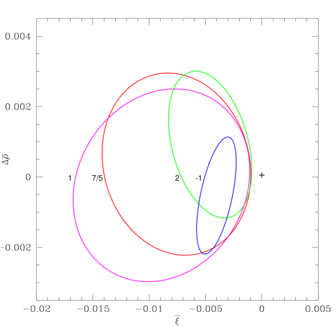
Figure 1: 99% C.L. contours for the four basic classes of models labeled by their $Q/u^{c}$ charge ratio in the $(\overline{\xi},\Delta\overline{\rho})$ plane. The cross represents the SM.

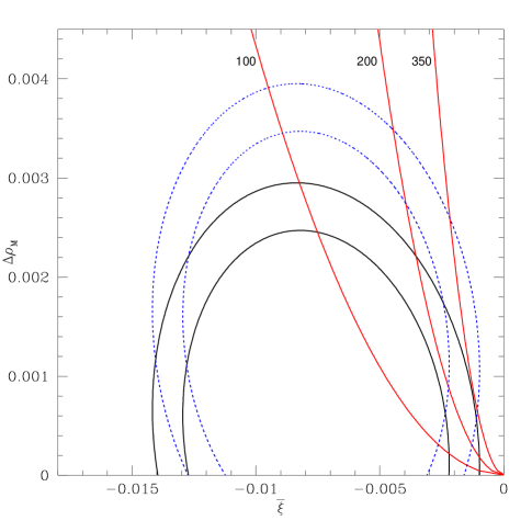
Figure 2: $\chi^{2}$ contours for the C(7/5) Model in the $(\overline{\xi},\Delta\rho_{M})$ plane. The solid ellipses represent the 95% and 99% C.L. bounds on the fit. The dashed ellipses represent the corresponding bounds if $\Delta\rho_{\rm extra}=-0.001$. The three solid lines are contours of $M_{Z^{\prime}}$ arising from the theoretical constraint of perturbativity of the $U(1)^{\prime}$ coupling up to the GUT scale, and are labeled in GeV.

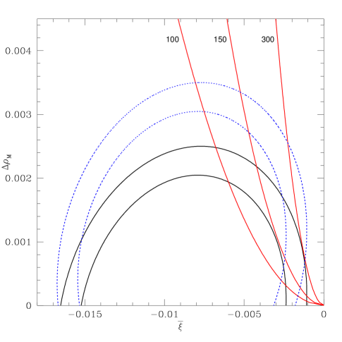
Figure 3: $\chi^{2}$ contours for the C(1) Model in the $(\overline{\xi},\Delta\rho_{M})$ plane. See caption of Figure 2 for explanation.

4 The $\eta$-model

As we noted in Section 1, $E_{6}$ is a natural, and for our purposes, minimal, choice for a simple GUT group containing extra $U(1)$’s. In addition $E_{6}$ appears as an underlying feature in many geometric compactifications of the $E_{8}\times E_{8}$ heterotic string. In either case, the list of possible subgroups into which the $E_{6}$ can break is small and well-defined.

Since $E_{6}$ is rank-6, its Cartan subalgebra contains two $U(1)$ generators besides those of the SM gauge groups. At scales just above the electroweak scale, the additional gauge symmetry could appear either as a commuting $U(1)^{\prime}$ factor (as we have been assuming up to this point) or as a unification of the SM groups into some non-Abelian group (e.g., $SU(4)_{c}\times SU(2)_{L}\times SU(2)_{R}$). The latter choice cannot describe the physics at LEP since it cannot be leptophobic. Returning to the former, we can write the new $U(1)^{\prime}$ as a combination of the two extra $U(1)$’s in $E_{6}$, usually denoted as $U(1)_{\chi}$ and $U(1)_{\psi}$:

$$Q^{\prime}(\alpha)=\cos\alpha\,Q_{\chi}+\sin\alpha\,Q_{\psi}.$$ (50)

In Table 4 the charges $Q_{\chi}$ and $Q_{\psi}$ are given for each of the states of the MSSM using the standard embedding into the ${\bf 27}$.

	$\sqrt{\frac{5}{3}}\,Y$	$2\sqrt{6}\,Q_{\psi}$	$2\sqrt{10}\,Q_{\chi}$	$2\sqrt{15}\,Q_{\eta}$
$Q$	$1/6$	1	$-1$	$-2$
$u^{c}$	$-2/3$	1	$-1$	$-2$
$d^{c}$	$1/3$	1	3	1
$L$	$-1/2$	1	3	1
$e^{c}$	1	1	$-1$	$-2$
$H_{u}$	$1/2$	$-2$	2	4
$H_{d}$	$-1/2$	$-2$	$-2$	1
$D$	$-1/3$	$-2$	2	4
$D^{c}$	1/3	$-2$	$-2$	1
$\nu^{c}$	0	1	$-5$	$-5$
$S$	0	4	0	$-5$

Table 4: $U(1)$ charges of the states of a ${\bf 27}$ of $E_{6}$.

No linear combination of $U(1)_{\chi}$ and $U(1)_{\psi}$ is completely leptophobic. The best one can do is to find models for which the axial coupling of the charged leptons is zero. Since the vectorial contributions for charged leptons appear proportional to $1-4s^{2}_{W}\simeq 0.07$, the $Z^{\prime}$ coupling to charged leptons could be highly suppressed with respect to the hadronic couplings. However, such models would necessarily have couplings to the neutrinos of order the hadronic couplings. If, after $Z$-$Z^{\prime}$ mixing the net effect were an increase in $\Gamma_{\rm inv}$ at LEP, the model could be quickly ruled out. On the other hand, if $\Gamma_{\rm inv}$ were to decrease, one could imagine that some new source of invisible $Z$-decays (e.g., neutralinos) could offset the difference. We consider such a scenario to be fine tuned and do not consider it here.

However, as was discussed in Section 2.1, in an arbitrary $U(1)_{a}\times U(1)_{b}$ model, there is one more free parameter, a mixing parameter $g_{ab}$ for the two groups. In the case of the breaking of some unified gauge group, $G_{\rm GUT}$, at some high scale into $G_{\rm GUT}\to SU(3)_{c}\times SU(2)_{L}\times U(1)_{Y}\times U(1)^{\prime}$, the value of $g_{ab}$ will be zero at the high scale. Nonetheless, through its RGE’s, Eq. (24), $g_{ab}$ will be driven to non-zero values for generic particle content. The effective coupling to the $Z^{\prime}$ is then $Q_{\rm eff}=Q^{\prime}(\alpha)+\delta\,Y$ where $\delta=g_{ab}/g^{\prime}$.

From the low-energy point of view, $\delta$ is a completely free parameter which must be fit to the data just as we did $\overline{\xi}$ or $\Delta\rho$. Therefore, we have repeated the $\chi^{2}$ analysis of the previous Section; however the charges of the SM fermions are now completely determined in terms of $\alpha$ instead of $x$ and $y$. Figure 4 is a $\chi^{2}$ plot in the plane of $(\alpha,\delta)$ showing the fits to the LEP data at 95% and 99% C.L. At each point in the plane, the $\chi^{2}$ value is minimized with respect to the remaining two free parameters, $\Delta\rho$ and $\overline{\xi}$. Along the bottom of the plot are indicated the values of $\alpha$ consistent with the $\chi$, $\psi$, and $\eta$ models ($\alpha=0$, $\pi/2$, $-\tan^{-1}\sqrt{5/3}\simeq-0.91$ respectively) commonly discussed in the literature. All previous discussions of these models (with the exception of Ref. [23]) have tacitly taken $\delta=0$.

What is remarkable about the fit is that it picks a very particular model out, for a limited range of $\delta$. To fall within the 95% C.L. region ($\chi^{2}\leq 14.1$), a model must have $\alpha=-0.89\pm 0.06$ and $\delta=0.35\pm 0.08$. Recall that the SM has a $\chi^{2}=22.8$ in the same parameterization. Only one model lies within the region of allowed $\alpha$: the so-called $\eta$-model. The charges of the MSSM states under $U(1)_{\eta}$ are given in Table 4.

That the best fit in the ($\alpha,\delta$) plane lies at $Q^{\prime}\simeq Q_{\eta}$ and $\delta\simeq 1/3$ is not surprising. The effective charge $Q_{\rm eff}=Q_{\eta}+Y/3$ is completely leptophobic; in fact it is the only combination of the three Abelian generators in $E_{6}$ which is leptophobic. Note that the $Q_{\eta}$ charges of the lepton doublet $L$ and the lepton singlet $e^{c}$ are proportional to their hypercharges. Thus, $U(1)_{\eta}$ is uniquely picked out as capable of describing the new physics at LEP. In Figure 4 we have shown the $\delta=1/3$ $\eta$-model with a cross.

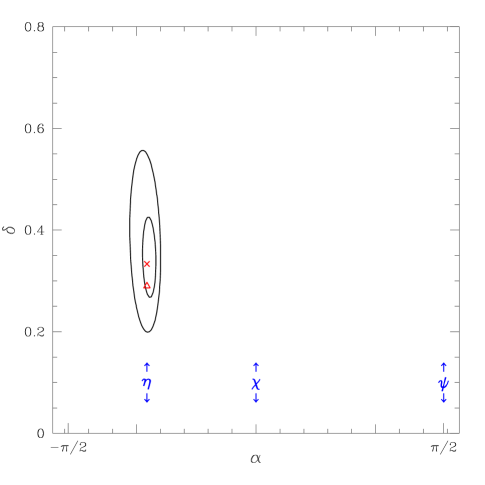
Figure 4: $\chi^{2}$ contours for general $E_{6}$ models. The two contours represent confidence levels of 95% and 99%. Three canonical $E_{6}$ models are labeled at the bottom. The two points highlight the $\eta$-model with $\delta=1/3$ (${\bf\times}$) and $\delta=0.29$ (${\bf\triangle}$).

If $U(1)^{\prime}$ is indeed $U(1)_{\eta}$, there are a number of direct consequences both for theory and phenomenology. First, $U(1)_{\eta}$ does not fit into any GUT group smaller than $E_{6}$. Thus, if the unification of the gauge couplings at a scale near $10^{16}\,{\rm GeV}$ is not an accident, it indicates either a true field-theoretic $E_{6}$ GUT (and no $SU(5)$ or $SO(10)$ unification) or string-type unification in which $SU(3)\times SU(2)_{L}\times U(1)_{Y}\times U(1)_{\eta}$ unifies directly at the scale $M_{\rm MSSM}=2\times 10^{16}~{}\,{\rm GeV}$. Second, cancellation of the anomalies in Eqs. (34)–(37) requires the existence of three complete 27’s of $E_{6}$. Besides the usual states of the MSSM, one can expect three pairs of $D$ and $D^{c}$ quarks which are $SU(2)_{L}$ singlets with $Y=\mp 1/3$, two additional pairs of $SU(2)_{L}$ doublets with $Y=\pm 1/2$, three right-handed neutrinos, $\nu^{c}_{i}$, plus SM singlets (at least one of which will receive a vev to break $U(1)_{\eta}$ and will be eaten by the $Z^{\prime}$).

We can now write the mass matrix of the $Z$-$Z^{\prime}$ system. Defining $\tan\beta\equiv\left\langle H_{u}\right\rangle/\left\langle H_{d}\right\rangle$ and $g_{\eta}$ to be $E_{6}$-normalized, the off-diagonal element in the mass matrix is given as in Eq. (12):

$$\Delta m^{2} = \frac{2g_{2}g^{\prime}}{c_{W}}\sum_{i}\left\langle T_{3i}\phi_{i}\right\rangle\left\langle(Q_{\eta}+\delta\,Y)\phi_{i}\right\rangle$$ (51)

$$= -\frac{1}{2c_{W}}\sqrt{\frac{5}{3}}g_{\eta}g_{2}v_{Z}^{2}\sin^{2}\beta$$

where the last equality holds for the case where the only $SU(2)_{L}$ doublets with non-zero vev’s are $H_{u}$ and $H_{d}$. For the completely leptophobic $\eta$-model (i.e., $\delta=1/3$), $\overline{\xi}$ and $\Delta\rho_{M}$ are then simply

$$\overline{\xi}=\frac{g^{2}_{\eta}c^{2}_{W}}{g_{2}^{2}}\sqrt{\frac{5}{3}}\sin^{2}\beta\left(\frac{M_{Z}^{2}}{M_{Z^{\prime}}^{2}}\right),\quad\quad\Delta\rho_{M}=\sqrt{\frac{5}{3}}\sin^{2}\beta\,\overline{\xi}\left(1-\frac{1}{15\sin^{4}\beta}\right).$$ (52)

Unfortunately, such a relationship between $\Delta\rho_{M}$ and $\overline{\xi}$ does not provide a very good fit to the data except near the unphysical value of $\tan\beta\simeq 0.6$; the best fit consistent with Eq. (52) and $\tan\beta>1$ has $\chi^{2}$ of 22.0, not much better than the SM $\chi^{2}=22.8$. There is a second related problem: since $\Delta m^{2}\sim M_{Z}^{2}$ and we expect (in the absence of tuning) for the $Z^{\prime}$ mass to be only somewhat heavier, we should expect large mixing angles $\xi$ to result. This is generic problem of $U(1)^{\prime}$ models where the $U(1)^{\prime}$ is expected to be radiatively broken close to the weak scale [24].

The solution to both problems involves the introduction of additional $SU(2)_{L}$ doublets, charged under $U(1)^{\prime}$, which receive vev’s near the weak scale. In our case these will play several roles: arranging the $\beta$-functions of the model to unify at the GUT scale, allowing for small $\xi$ by cancelling the $H_{u}$ contribution to $\Delta m^{2}$, likewise decoupling $\Delta\rho_{M}$ from $\overline{\xi}$, and driving $\delta>0$.

Consider, for example, extending the minimal $\eta$-model to include the pair of doublets which fit into the $[{\bf 78},{\bf 16+\overline{16}},{\bf\overline{5}}+{\bf 5}]$ of $[E_{6},SO(10),SU(5)]$, with the doublet in the ${\bf 5}$ getting a vev, $v_{\ell}$, near the weak scale. Then in the leptophobic $\eta$-model, $\Delta m^{2}\propto(v_{Z}^{2}\sin^{2}\beta-v_{\ell}^{2})$. If a near cancellation can be arranged between the two terms in $\Delta m^{2}$, then small mixing will result and simultaneously $\Delta\rho_{M}\ll\overline{\xi}$ as needed phenomenologically. Since $M_{Z}^{2}\propto(v_{Z}^{2}+v_{\ell}^{2})$ and we need $v_{Z}$ and $v_{\ell}$ of the same order, the Higgs vevs, $v_{u}$ and $v_{d}$, which give masses to the fermions will be proportionally smaller. In the case $v_{d}\ll v_{u}\sim v_{\ell}$, the large top-bottom mass ratio is natural and the top Yukawa is of the same size as one would expect in the MSSM with $\tan\beta=1$. This is actually still below the top Yukawa infrared pseudo-fixed point, which now takes a larger value ($h_{t}^{\rm fixed}\simeq 1.25$) because of the slow running of $\alpha_{s}$ in this model.

Imposing on the superpotential of the minimal $\eta$-model a discrete $Z_{2}$ symmetry (a simple extension of the usual $R$-parity) one finds:

$$W_{\eta}=Qu^{c}H_{u}+Qd^{c}H_{d}+Le^{c}H_{d}+SH_{u}H_{d}+SDD^{c}+L\nu^{c}H_{u}$$ (53)

Under the $R$-parity, all the states of the ${\bf 27}$ are odd except $H_{u}$, $H_{d}$ and $S$. This superpotential forbids dimension-4 proton decay; dimension-5 operators are also known to be unobservably small in the $\eta$-model [25]. There appears in the superpotential a Yukawa mass term for the right-handed neutrino fields, $L\nu^{c}H_{u}$. To be consistent with current neutrino mass bounds, this coupling must be small or zero or the $\nu^{c}$ must have large Majorana mass terms through some singlets. By flipping the $R$-parity assignment of the $\nu^{c}$ one can forbid the term altogether, but at the price of introducing into the superpotential the term $\nu^{c}Dd^{c}$. Such a term would lead to $D$-$d^{c}$ mixing were $\nu^{c}$ to receive a non-zero vev.

One can also expect radiative symmetry breaking much as in the MSSM. If the $SDD^{c}$ coupling is ${\cal O}(1)$, the soft mass term for the $S$-field, $m_{S}^{2}$, will be driven negative through its RGE’s, triggering $U(1)_{\eta}$-breaking through $\left\langle S\right\rangle\neq 0$ at a scale just above the electroweak scale. (The electroweak symmetry will similarly be broken by $m^{2}_{H_{u}}$ running negative due to the large top Yukawa coupling.) Since the singlet $S$ has no electroweak interactions unlike $H_{u}$, it is conceivable that the mass-squared of the $S$ fields turns negative at a larger momentum scale compared to $H_{u}$. The non-zero $\left\langle S\right\rangle$ will in turn produce a $\mu H_{u}H_{d}$ and a $\mu^{\prime}DD^{c}$ term. For $SH_{u}H_{d}$ and $SDD^{c}$ couplings of ${\cal O}(1)$, one expects $\mu,\mu^{\prime}\sim M_{Z^{\prime}}$. In particular, it is natural for the $D$ and $D^{c}$ states to be heavier than the $Z$. Finally, we note that there is no mechanism within the $\eta$-model for $\nu^{c}$ to receive a vev radiatively which does not violate some other constraint (such as neutrino mass bounds) [25]. Thus $D$-$d^{c}$ mixing will not occur.

The $\eta$-model with only three ${\bf 27}$’s of $E_{6}$ does not satisfy all of our initial principles because it does not have gauge coupling unification. As mentioned above, unification can be arranged by introducing one pair of $SU(2)_{L}$ doublets with hypercharges $\sqrt{5/3}\,Q_{Y}=\pm\frac{1}{2}$. From a string point of view, these may be viewed as coming from a ${\bf\overline{27}}+{\bf 27}$ or a ${\bf 78}$, the rest of whose states received masses at the string scale [26]. This, along with anomaly cancellation considerations, requires the doublets to have equal and opposite $Q_{\eta}$. If these doublets also have non-zero effective charges $Q_{\eta}+\delta\,Y$, their vev’s may contribute to the $Z$-$Z^{\prime}$ mixing matrix as outlined above. A problem may potentially arise in trying to generate vev’s for these doublets radiatively; one possibility is to allow couplings of the type $H_{u}H_{d}^{\prime}$ through singlets.

(This model has, beyond the spectrum of the MSSM, three each of $({\bf 3,1})$ and $({\bf\overline{3},1})$ and six of $({\bf 1,2})$. This is exactly the content of three $({\bf\overline{5}}+{\bf 5})$’s of $SU(5)$. Note that in terms of the charge ratio $y/x$, the purely leptophobic ($\delta=1/3$) $\eta$-model is equivalent to Model A of Section 3. However, the presence of kinetic mixing ($\delta\neq 0$) induces contributions to the oblique electroweak parameters not present in Model A. Also unlike the purely leptophobic models of that Section the value of $\delta$ in the $\eta$-model is generically not $1/3$, but is instead determined through the RGE’s and thus through the low-energy spectrum. Further, its $\beta$-function is substantially smaller than that of Model A with a single $({\bf\overline{5}}+{\bf 5})$, since for the $\eta$-model the anomaly cancellation is generation by generation, providing a more economical set of charges.)

There are two variants of the $\eta$-model for which the value of $\delta$ at the electroweak scale is of particular interest: (i) The “minimal” $\eta$-model that possesses three generations of ${\bf 27}$’s and one additional vector-like pair of Higgs doublets that arises from the ${\bf 78}$ of $E_{6}$. These doublets have charges $\sqrt{5/3}\,Q_{Y}=-1/2$ and $2\sqrt{15}\,Q_{\eta}=6$ under the GUT-normalized $U(1)_{Y}\times U(1)_{\eta}$ symmetries; (ii) The “maximal” $\eta$-model with in addition to the states of the minimal $\eta$-model a further effective ${\bf\overline{5}}+{\bf 5}$ of $SU(5)$ is added (so that unification is preserved), but which is composed of a second vector-like pair of the doublets in the ${\bf 78}$ together with the color triplets $D+\overline{D}$ coming from the ${\bf 27}+{\bf\overline{27}}$. The maximal model has the largest field content consistent with perturbative unification of the gauge couplings at $2\times 10^{16}\,{\rm GeV}$. The values of the charge inner products $B_{ij}$ for these two models are given in Table 5. The field content of both these models is consistent with small $\Delta m^{2}$ in the $Z$-$Z^{\prime}$ mass matrix.

Model	$B_{YY}$	$B_{\eta\eta}$	$B_{Y\eta}$
$\eta_{\rm min}$	$9+\frac{3}{5}$	$9+\frac{12}{5}$	$-\frac{6}{5}$
$\eta_{\rm max}$	$9+\frac{8}{5}$	$9+\frac{32}{5}$	$-\frac{16}{5}$

Table 5: Beta-function coefficients for the Minimal and Maximal $\eta$-models, GUT normalized.

Running the SM couplings up to the unification point and then numerically running the RGE’s of Eq. (24) for $g_{Y}$, $g_{\eta}$ and $g_{Y\eta}$ down to the electroweak scale, we find predictions for $\delta$ in the two models:

$$\delta_{\rm min}=0.11,\quad\quad\quad\delta_{\rm max}=0.29.$$ (54)

Both of these are calculated with $\alpha_{s}(M_{Z})=0.120$. Larger values of $\alpha_{s}(M_{Z})$ lead to a slight increase in the values of $\delta$ compared to Eq. (54). The threshold corrections to $\delta$ coming from mass splitting of the light states are typically of order $0.01$. It is quite remarkable that the totally leptophobic value of $\delta=1/3$ is very nearly predicted by the renormalization group running of the “maximal” $\eta$-model. From the one-loop RGE’s, the value of the $U(1)_{\eta}$ gauge coupling at the electroweak scale is $g_{\eta}=0.40$.

Given these values of $\delta$ we can now investigate how well the $\eta$-model variants can fit the LEP data. As discussed in Section 2.2 we will consider both the case of $S_{\rm extra}=0$ and $S_{\rm extra}=0.14$ per pair of higgsino/lepton-like doublets. We will take $\Delta\rho_{\rm extra}=0$. The minimal model is clearly disfavored by the data, having a $\chi^{2}$ no better than the SM for both values of $S_{\rm extra}$. Likewise the maximal model with $S_{\rm extra}=0$ is disfavored. The phenomenologically favored maximal model has 5 doublet pairs giving $S_{\rm extra}=0.7$ and a minimum $\chi^{2}=13.9$ at a $Z^{\prime}$ mass of $215\,{\rm GeV}$; this is within the 95% C.L. bounds shown in Figure 4, where the model is indicated by a triangle. At the minimum, $S\equiv S_{M}+S_{\rm extra}=-0.1$. Note that the goodness of the fit does not depend strongly on the exact value of $S_{\rm extra}$ in the range 0.5 to 1.5; in particular the resulting $S$ only varies within the range $-0.1$ to $0.1$.

Given $g_{\eta}$ and the bounds on $\Delta\rho_{M}$ and $\overline{\xi}$ we are in a position to calculate the bounds on the $Z^{\prime}$ mass, using Eq. (13). For the $\eta$-model with $\delta=0.29$, we find that in order to fall within the 95% (99%) C.L. limits for our fit, then $M_{Z^{\prime}}\leq 240\,(420)\,{\rm GeV}$, under the assumption of no additional contributions to $\Delta\overline{\rho}$. (New positive contributions to $\Delta\overline{\rho}$, which are natural in these models, push the best fit $Z^{\prime}$ mass to lower values.) These fits are shown in Figure 5. UA2 has performed a $Z^{\prime}$ search in the dijet channels, excluding a $Z^{\prime}$ with 100% branching fraction to hadrons and SM strength interactions up to masses of $260\,{\rm GeV}$ [22]. However, given the value of $g_{\eta}=0.4$ and the $U(1)_{\eta}$ charges of the quarks, one can show that the production cross-section for this $Z^{\prime}$ is approximately 1/4 that of the $Z$, too small to be excluded at UA2.

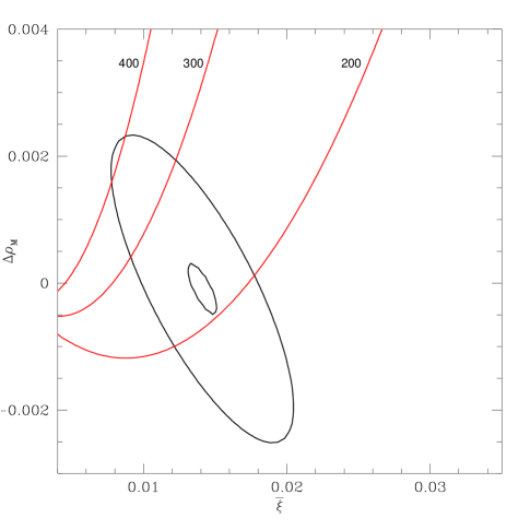
Figure 5: $\chi^{2}$ contours for the $\eta$-model with $\delta=0.29$ in the $(\overline{\xi},\Delta\rho_{M})$ plane. See caption of Figure 2 for explanation. Additional positive contributions to $\Delta\overline{\rho}$ reduce the best fit value of the $Z^{\prime}$ mass.

What is remarkable about this analysis is that the $\eta$-model, which has been extensively studied in the literature and for which strong bounds on its mixing with the $Z$ and its mass have been published, has been resuscitated by the inclusion of the additional $U(1)$ kinetic mixing effect. This is even more so, since the value of $\delta$ is correctly predicted in specific models in which only one discrete choice of matter content has been made!

5 Conclusions

In this paper, we have investigated the possibility of explaining the $R_{b}$ excess – $R_{c}$ deficit reported by the LEP experiments through $Z$-$Z^{\prime}$ mixing effects. We have constructed a set of models consistent with a restrictive set of principles: unification of the SM gauge couplings, vector-like additional matter, and couplings which are both generation-independent and leptophobic. These models are anomaly-free, perturbative up to the GUT scale, and contain realistic mass spectra. Out of this class of models, we find three explicit realizations (the $\eta$, C(7/5), and C(1) models) which fit the LEP data to a far better extent than the unmodified SM or MSSM and satisfy all other phenomenological constraints which we have investigated. The $\eta$-model is particularly attractive, coming naturally from geometrical compactifications of heterotic string theory. This is especially so since the value of the mixing parameter, $\delta$, is correctly predicted given only one discrete choice of matter content.

In general, these models predict extra matter below $1\,{\rm TeV}$ and $Z^{\prime}$ gauge bosons below about $500\,{\rm GeV}$, though the $Z^{\prime}$ of these models will be difficult to detect experimentally.

Note Added

After this work was completed two further interesting works concerning the experimental consequences of leptophobic $U(1)$’s appeared [28][29]. These papers noted that there can exist important low-energy constraints on leptophobic models arising from atomic parity violation (APV) and deep-inelastic neutrino scattering experiments. In particular, Ref. [28] argued that the aesthetically appealing models that we have constructed in this paper are strongly disfavored by the APV data. While this is usually true in the heavy $Z^{\prime}$ mass approximation that we have been employing up to now, this conclusion does not hold in the very interesting case of a light $Z^{\prime}$ ($M^{2}_{Z^{\prime}}\ \raise 1.29167pt\hbox{$>$\kern-7.5pt\lower 4.30554pt\hbox{$\sim$}}\ m^{2}_{Z}$), as we will now outline.

The APV experiments result in constraints on the so-called weak nuclear charge $Q_{W}$ of various elements such as Cesium and Thallium with high atomic and neutron numbers $Z$ and $N$. The charge $Q_{W}$ is itself defined in terms of the product of the axial electron coupling with the up and down type quark vector coupling via $Q_{W}=-2\left\{C_{1u}(2Z+N)+C_{1d}(Z+2N)\right\}$ where

$${\cal L}_{NC}=-{G_{F}\over\sqrt{2}}\sum_{i=u,d}C_{1i}(\overline{e}\gamma_{\mu}\gamma_{5}e)(\overline{q}_{i}\gamma^{\mu}q_{i})+\cdots$$

In the case where the $M_{Z^{\prime}}\sim m_{Z}$, both $Z_{1}$ and $Z_{2}$ exchange contribute to the coefficients $C_{1i}$. In the approximation where the mixing is small $\xi\ll 1$, but no expansion is made in the mass ratio $r\equiv(m^{2}_{Z}/M^{2}_{Z^{\prime}})$, the expression for the $C_{1i}$’s is

$$C_{1i}=-\left\{v_{i}+v^{{}^{\prime}}_{i}\overline{\xi}(1-r)\right\},$$

where the $v$’s and $\overline{\xi}$ are defined in Eqs. (4) and (9) respectively. It is therefore clear that the constraint from the APV data becomes vacuous as $r\to 1$. Specifically, we find that the APV data do not significantly increase the total $\chi^{2}$ for $Z^{\prime}$ masses below about $150~{}\,{\rm GeV}$.

One may similarly consider the effect of a leptophobic $Z^{\prime}$ on the neutrino scattering experiments. We find that the parameters $\varepsilon^{i}_{L}$ and $\varepsilon^{i}_{R}$ defined in Ref. [30], are altered by an amount

$$\Delta\varepsilon^{i}_{L/R}=\left({v^{{}^{\prime}}_{i}\mp a^{{}^{\prime}}_{i}\over 2}\right)\overline{\xi}(1-r),$$

respectively. Thus the weaker constraints from the neutrino scattering data also dissappear for light to moderate $Z^{\prime}$ masses.

We will address the full fit including these constraints (as well as the SLC and other data), more fully in a forthcoming paper Ref. [31], where we will also discuss the models with variant Higgs structure mentioned in the Section 3 footnote.

References

- [1] LEP Electroweak Working Group, report LEPEWWG/95-02 (August 1995).
- [2] All calculations in this paper were done using the Z0POLE program of B. Kniehl and R. Stuart, Comput. Phys. Commun. 72 (1992) 175.
- [3] F. Abe, et al.(CDF Collaboration), Phys. Rev. Lett. 74 (1995) 2626.
-
[4]
J. Wells, C. Kolda and G. Kane, Phys. Lett. B338 (1994) 219;
D. Garcia, R. Jimenez and J. Sola, Phys. Lett. B347 (1995) 321;
E. Simmons and Y. Su, report BUHEP-96-4 (February 1996) [hep-ph/9602267]. -
[5]
B. Holdom, Phys. Lett. B339 (1994) 114; Phys. Lett. B351 (1995) 279;
X. Zhang and B.L. Young, Phys. Rev. D51 (1995) 6584;
E. Ma and D. Ng, Phys. Rev. D53 (1996) 255;
M. Carena, H.E. Haber and C. Wagner, report CERN-TH-95-311 (December 1995) [hep-ph/9512446];
T. Yoshikawa, report HUPD-9528 (December 1995) [hep-ph/9512251];
P. Bamert, C. Burgess, J. Cline, D. London and E. Nardi, report MCGILL 96-04 (February 1996) [hep-ph/9602438]. -
[6]
E. Ma, UCRHEP-T-153 [hep-ph/9510289];
G. Bhattacharya, G. Branco and W-S. Hou, report CERN-TH/95-326 (December 1995) [hep-ph/9512239];
C.V. Chang, D. Chang and W-Y. Keung, report NHCU-HEP-96-1 (January 1996) [hep-ph/9601326]. - [7] J. Feng, H. Murayama and J. Wells, report SLAC-PUB-95-7089 (January 1996) [hep-ph/9601295].
- [8] G. Altarelli, N. di Bartolomeo, F. Feruglio, R. Gatto and M. Mangano, report CERN-TH-96-20 (January 1996) [hep-ph/9601324].
- [9] P. Chiappetta, J. Layssac, F. Renard and C. Verzegnassi, report PM-96-05 (January 1996) [hep-ph/9601306].
-
[10]
K. Dienes and A. Faraggi, Nucl. Phys. B457 (1995) 409;
K. Dienes, A. Faraggi and J. March-Russell, report IASSNS-HEP-95/25 (October 1995) [hep-th/9510223].
For a recent review of unification in the string framework see: K. Dienes, report IASSNS-HEP-95/97 (February 1996) [hep-th/9602045]. - [11] E. Witten, report IASSNS-HEP-96/08 (February 1996) [hep-th/9602070].
- [12] B. Holdom, Phys. Lett. B166 (1986) 196.
- [13] F. del Aguila, G. Coughlan and M. Quiros, Nucl. Phys. B307 (1988) 633.
- [14] For a review, see J. Hewett and T. Rizzo, Phys. Rep. 183 (1989) 193.
- [15] G. Altarelli, R. Casalbuoni, D. Dominici, F. Feruglio and R, Gatto, Mod. Phys. Lett. A5 (1990) 495.
- [16] B. Holdom, Phys. Lett. B259 (1991) 329.
-
[17]
R. Foot and X-G. He, Phys. Lett. B267 (1991) 509;
F. del Aguila, M. Masip and M. Perez-Victoria, report UG-FT-46-94 (July 1995) [hep-ph/9507455]. - [18] M. Drees and K. Hagiwara, Phys. Rev. D42 (1990) 1709.
-
[19]
R. Barbieri, M. Frigeni, F. Giuliani, and H. Haber,
Nucl. Phys. B341 (1990) 309;
G. Altarelli, R. Barbieri, and F. Caravaglios, Phys. Lett. B314 (1993) 357. - [20] E. Ma and P. Roy, Phys. Rev. Lett. 68 (1992) 2879.
- [21] F. Abe, et al., (CDF Collaboration), Phys. Rev. Lett. 74 (1995) 3539.
- [22] J. Alitti, et al., (UA2 Collaboration), Nucl. Phys. B400 (1993) 3.
- [23] F. del Aguila, M. Cvetič and P. Langacker, Phys. Rev. D52 (1995) 37.
- [24] M. Cvetič and P. Langacker, report IASSNS-HEP-95/90 (November 1995) [hep-ph/9511378].
- [25] B. Campbell, J. Ellis, K. Enqvist, M. Gaillard and D. Nanopoulos, Int. J. Mod. Phys. A2 (1987) 831.
- [26] E. Witten, Nucl. Phys. B258 (1985) 75.
- [27] F. del Aguila, M. Quiros and F. Zwirner, Nucl. Phys. B287 (1987) 419.
- [28] K. Agashe, M. Graesser, I. Hinchliffe and M. Suzuki, report LBL-38569 (April 1996), [hep-ph/9604266].
- [29] V. Barger, K. Cheung and P. Langacker, report MADPH-96-936 (April 1996), [hep-ph/9604298].
- [30] L. Montanet, et al., (Particle Data Group), Phys. Rev. D50 (1994) 1173, Section 26.2.
- [31] K. S. Babu, C. Kolda and J. March-Russell, report IAS-HEP-96/45 (in preparation).