CEBAF-TH-96-01                                                                              BNL-

Abstract: A study of $R_{b}$ and $R_{c}$ is presented in the context of a Two Higgs Doublet Model (2HDM) with flavor changing scalar currents (FCSC). Implications of the model for the $\rho$-parameter and for $b\to s\gamma$ are also considered. The experimental data on $R_{b}$ places stringent constraints on the model parameters. The configuration of the model needed to account for $R_{b}$ is found to be irreconcilable with constraints from $b\to s\gamma$ and $\rho$. In particular, if $R^{\rm exp}_{b}>R^{\scriptscriptstyle{\rm SM}}_{b}$ persists then this version of 2HDM will be ruled out or require significant modifications. Noting that aspects of the experimental analysis for $R_{b}$ and $R_{c}$ may be of some concern, we also disregard $R^{\rm exp}_{b}$ and $R^{\rm exp}_{c}$ and give predictions for these using constraints from $b\to s\gamma$ and $\rho$ parameter only. We emphasize the theoretical and experimental advantages of the observable $R_{b+c}\equiv\Gamma(Z\to b\bar{b}\mbox{ or }c\bar{c})/\Gamma(Z\to\mbox{hadrons})$. We also stress the role of $R_{\ell}\equiv\Gamma(Z\to\mbox{hadrons})/\Gamma(Z\to\ell^{+}\ell^{-})$ in testing the Standard Model (SM) despite its dependence on QCD corrections. Noting that in models with FCNC the amplitude for $Z\to c\bar{c}$ receives a contribution which grows with $m^{2}_{t}$, the importance and uniqueness of precision $Z\to c\bar{c}$ measurements for constraining flavor changing $t\bar{c}$ currents is underscored.

1 Introduction and Summary

For the past several years precision studies at LEP have been providing important confirmation to various aspects of the Standard Model (SM) [1]. A notable exception that has emerged is the decay of $Z\to b\bar{b}$. It has long been recognized that the $Zb\bar{b}$ vertex is very sensitive to effects of virtual, heavy particles [2]. Consequently, a deviation from the prediction of the SM could prove to be a significant clue to new physics. It is, therefore, clearly important to study $Z\to b\bar{b}$ in extensions of the SM [3] and pursue the resulting implications. In this paper we study these decays in a class of Two-Higgs-Doublet Models (2HDM), called Model III [4]-[10], which present a natural mechanism for flavor changing scalar currents (FCSC).

Our focus is the branching ratio of $Z\to b\bar{b}$, i.e. [1]

$$R_{b}\equiv\frac{\Gamma(Z\to b\bar{b})}{\Gamma(Z\to\hbox{hadrons})}$$ (1)

It is worth noting that, since $R_{b}$ is a ratio between two hadronic rates, most of the electroweak (EW) oblique and QCD corrections cancel between numerator and denominator, making it a uniquely clean and sensitive test of the SM. Experiment finds [1]:

$$R^{\rm exp}_{b}=.2205\pm.0016$$ (2)

whereas the SM prediction is [1]

$$R^{\scriptscriptstyle{\rm SM}}_{b}=.2156$$ (3)

The difference, of about 3$\sigma$, is a possible indication of new physics. We note, in passing, that the related decay $Z\to c\bar{c}$ has also been measured albeit with appreciably less precision [1]

$$R^{\rm exp}_{c}=.1543\pm.0074$$ (4)

The SM prediction, on the other hand, is [1]

$$R^{\scriptscriptstyle{\rm SM}}_{c}=.1724$$ (5)

Thus $R^{\rm exp}_{c}$ also appears not to be consistent with the SM although the deviation is milder (about $2.3\sigma$). It is interesting to note that whereas $R^{\rm exp}_{b}$ is larger than $R^{\scriptscriptstyle{\rm SM}}_{b}$, $R^{\rm exp}_{c}$ is less than the SM expectation. Note also that $R^{\rm exp}_{b}$ quoted above is obtained by holding $R_{c}$ fixed to its SM value [1].

Our findings are that if we take $R^{\rm exp}_{b}$ at its face value then, while Model III can accommodate $R^{\rm exp}_{b}$, the model parameters get severely constrained. In particular, the resulting configuration of the model cannot be reconciled with the constraints from the $\rho$-parameter and $Br(B\to X_{s}\gamma)$.

Several aspects of the $R_{b}$, $R_{c}$ experimental analysis are, though, of concern. The results given above in eqs. (2) and (4), include systematic errors and emerge from combining the numbers from the four LEP detectors [1]. Since some of the assumptions are common, treatment of the systematics can be problematic. Also the errors for $R_{b}$ and $R_{c}$ are correlated [1]. Indeed $R^{\rm exp}_{b}+R^{\rm exp}_{c}$ is consistent with the SM accentuating the possibility that part of the effect may well be resulting from misidentification of the flavors. In addition, the observable $R_{\ell}$,

$$R_{\ell}\equiv\frac{\Gamma(Z\to\mbox{hadrons})}{\Gamma(Z\to\ell^{+}\ell^{-})}$$ (6)

which is measured much more precisely than $R_{b}$ or $R_{c}$ and can be predicted in the SM using $\alpha_{s}(M_{Z})$ deduced from other methods (e.g. lattice and/or event shapes in $e^{+}e^{-}$ annihilation), is found not to be inconsistent with the SM, at present.

In light of these reservations we also fix the parameter space by using only the $\rho$-parameter and $Br(B\to X_{s}\gamma)$ and predict $R_{b}$, $R_{c}$ and $R_{b+c}$ in Model III. In particular, in this model, with constraints from the $\rho$-parameter and $Br(B\to X_{s}\gamma)$, we find that $R_{b}$ cannot exceed $R^{\scriptscriptstyle{\rm SM}}_{b}$. Thus, if the current trend in the experimental numbers (i.e. $R^{\rm exp}_{b}>R^{\scriptscriptstyle{\rm SM}}_{b}$) persists, this class of 2HDM will be either entirely ruled out or require a significant alteration.

In passing we also emphasize the advantages of the observable $R_{b+c}$

$$R_{b+c}=\frac{\Gamma(Z\to b\bar{b}\mbox{ or }c\bar{c})}{\Gamma(Z\to\mbox{hadrons})}$$ (7)

and give the predictions from Model III for $R_{b+c}$.

Finally, we stress the importance of precision determinations of $Z\to c\bar{c}$ (i.e. $R_{c}$). In type III models its amplitude receives a contribution which grows with $m^{2}_{t}$. A precise determination of $Z\to c\bar{c}$, thus, constitutes a uniquely clean method for constraining the flavor-changing $tc$ vertex that is of crucial theoretical concern.

2 Two Higgs Doublet Model with Flavor
Changing Currents

A mild extension of the SM with one additional scalar SU(2) doublet opens up the possibility of FCSC. For this reason, the 2HDM scalar potential is usually constrained by an ad hoc discrete symmetry [11], whose only role is to protect the model from tree-level FCSC. As a result one gets the so called Model I and Model II, when up-type and down-type quarks are coupled to the same or to two different doublets respectively [12]. In particular, it is to be stressed that from a purely phenomenological point of view, low energy experiments involving $K^{0}$-$\bar{K}^{0}$, $B^{0}$-$\bar{B}^{0}$ mixing, $K_{L}\to\mu\bar{\mu}$ etc. place very stringent constraints only on the existence of those tree level flavor changing transitions which directly involve the first family. Indeed, in view of the extraordinary mass scale of the top quark, it has been emphasized by many that anomalously large flavor-changing (FC) couplings involving the third family may exist [4]-[10],[13]. Thus, following Cheng and Sher [4], perhaps a natural way to limit the strength of the FCSC involving the first family is to assume that they are proportional to the masses of the participating quarks. In this way, the FC couplings are automatically put in a hierarchical order and the third family may well play an enhanced role.

For this type of 2HDM, the Yukawa Lagrangian for the quark fields can be taken to have the form [8, 9]

$${\cal L}^{(III)}_{Y}=\eta^{U}_{ij}\bar{Q}_{i,L}\tilde{\phi}_{1}U_{j,R}+\eta^{D}_{ij}\bar{Q}_{i,L}\phi_{1}D_{j,R}+\xi^{U}_{ij}\bar{Q}_{i,L}\tilde{\phi}_{2}U_{j,R}+\xi^{D}_{ij}\bar{Q}_{i,L}\phi_{2}D_{j,R}\,+\,h.c.$$ (8)

where $\phi_{i}$, for $i=1,2$, are the two scalar doublets of a 2HDM, while $\eta^{U,D}_{ij}$ and $\xi_{ij}^{U,D}$ are the non diagonal coupling matrices. For convenience we can choose to express $\phi_{1}$ and $\phi_{2}$ in a suitable basis such that only the $\eta_{ij}^{U,D}$ couplings generate the fermion masses, i.e. such that

$$<\phi_{1}>=\left(\begin{array}[]{c}0\\ {v/\sqrt{2}}\end{array}\right)\,\,\,\,,\,\,\,\,<\phi_{2}>=0$$ (9)

The two doublets are in this case of the form

$$\phi_{1}=\frac{1}{\sqrt{2}}\left\{\left(\begin{array}[]{c}0\\ v+H^{0}\end{array}\right)+\left(\begin{array}[]{c}\sqrt{2}\,\chi^{+}\\ i\chi^{0}\end{array}\right)\right\}\,\,\,\,;\,\,\,\,\phi_{2}=\frac{1}{\sqrt{2}}\left(\begin{array}[]{c}\sqrt{2}\,H^{+}\\ H^{1}+iH^{2}\end{array}\right)$$ (10)

The scalar Lagrangian in the ($H^{0}$, $H^{1}$, $H^{2}$, $H^{\pm}$) basis is such that[14, 12]:

1. the doublet $\phi_{1}$ corresponds to the scalar doublet of the SM and $H^{0}$ to the SM Higgs field (same couplings and no interactions with $H^{1}$ and $H^{2}$);

2. all the new scalar fields belong to the $\phi_{2}$ doublet;

3. both $H^{1}$ and $H^{2}$ do not have couplings to the gauge bosons of the form $H^{1,2}ZZ$ or $H^{1,2}W^{+}W^{-}$.

However, while $H^{\pm}$ is also the charged scalar mass eigenstate, ($H^{0}$, $H^{1}$, $H^{2}$) are not the neutral mass eigenstates. Let us denote by ($\bar{H}^{0}$, $h^{0}$) and $A^{0}$ the two scalar plus one pseudoscalar neutral mass eigenstates. They are obtained from ($H^{0}$, $H^{1}$, $H^{2}$) as follows

$$\bar{H}^{0} = \left[(H^{0}-v)\cos\alpha+H^{1}\sin\alpha\right]$$

$$h^{0} = \left[-(H^{0}-v)\sin\alpha+H^{1}\cos\alpha\right]$$ (11)

$$A^{0} = H^{2}$$

where $\alpha$ is a mixing angle, such that for $\alpha\!=\!0$, ($H^{0}$, $H^{1}$, $H^{2}$) coincide with the mass eigenstates. We find more convenient to express $H^{0}$, $H^{1}$ and $H^{2}$ as functions of the mass eigenstates, i.e.

$$H^{0} = \left(\bar{H}^{0}\cos\alpha-h^{0}\sin\alpha\right)+v$$

$$H^{1} = \left(h^{0}\cos\alpha+\bar{H}^{0}\sin\alpha\right)$$ (12)

$$H^{2} = A^{0}$$

In this way we may take advantage of the mentioned properties (1), (2) and (3), as far as the calculation of the contribution from new physics goes. In particular, only the $\phi_{1}$ doublet and the $\eta^{U}_{ij}$ and $\eta^{D}_{ij}$ couplings are involved in the generation of the fermion masses, while $\phi_{2}$ is responsible for the new couplings.

After the rotation that diagonalizes the mass matrix of the quark fields, the FC part of the Yukawa Lagrangian looks like

$${\cal L}_{Y,FC}^{(III)}=\hat{\xi}^{U}_{ij}\bar{Q}_{i,L}\tilde{\phi}_{2}U_{j,R}+\hat{\xi}^{D}_{ij}\bar{Q}_{i,L}\phi_{2}D_{j,R}\,+\,h.c.$$ (13)

where $Q_{i,L}$, $U_{j,R}$ and $D_{j,R}$ denote now the quark mass eigenstates and $\hat{\xi}_{ij}^{U,D}$ are the rotated couplings, in general not diagonal. If we define $V_{L,R}^{U,D}$ to be the rotation matrices acting on the up- and down-type quarks, with left or right chirality respectively, then the neutral FC couplings will be

$$\hat{\xi}^{U,D}_{\rm neutral}=(V_{L}^{U,D})^{-1}\cdot\xi^{U,D}\cdot V_{R}^{U,D}$$ (14)

On the other hand for the charged FC couplings we will have

$$\hat{\xi}^{U}_{\rm charged}\! = \!\hat{\xi}^{U}_{\rm neutral}\cdot V_{\scriptscriptstyle{\rm CKM}}$$

$$\hat{\xi}^{D}_{\rm charged}\! = \!V_{\scriptscriptstyle{\rm CKM}}\cdot\hat{\xi}^{D}_{\rm neutral}$$ (15)

where $V_{\scriptscriptstyle{\rm CKM}}$ denotes the Cabibbo-Kobayashi-Maskawa matrix. To the extent that the definition of the $\xi^{U,D}_{ij}$ couplings is arbitrary, we can take the rotated couplings as the original ones. Thus, we will denote by $\xi^{U,D}_{ij}$ the new rotated couplings in eq. (14), such that the charged couplings in (15) look like $\xi^{U}\cdot V_{\scriptscriptstyle{\rm CKM}}$ and $V_{\scriptscriptstyle{\rm CKM}}\cdot\xi^{D}$.

We will assume that the $\xi^{U,D}_{ij}$ couplings are purely phenomenological parameters and compare the region of the parameter space that could accommodate $R^{\rm exp}_{b}$ with the constraints from other physical processes. For convenience, we parametrize the $\xi^{U,D}_{ij}$ couplings in such a way as to make the comparison with the other 2HDM easier

$$\xi^{U,D}_{ij}=\lambda_{ij}\,\frac{\sqrt{m_{i}m_{j}}}{v}$$ (16)

This is very similar to what was proposed and used in ref. [4, 8, 9, 10], but we want now to allow the factors $\lambda_{ij}$ to vary over a broad range, constrained by phenomenology only. In this way we may be able to see if the experiment data lead to some new patterns in the coupling behavior [15].

3 Implications for $R_{b}$ and $R_{c}$

Let us now focus on the calculation of $R_{b}$ and $R_{c}$. The main task is to compute the corrections from new physics to the SM $Zq\bar{q}$ vertex, for $q=c,\,b$. Suppose the reference SM vertex for a $Z\to q\bar{q}$ process is

$$V_{q\bar{q}Z}^{\scriptscriptstyle{\rm SM}}\equiv-i\frac{g_{\scriptscriptstyle W}}{c_{\scriptscriptstyle W}}\bar{q}\gamma_{\mu}\left[\Delta_{q,L}^{\scriptscriptstyle{\rm SM}}\frac{(1-\gamma_{5})}{2}+\Delta_{q,R}^{\scriptscriptstyle{\rm SM}}\frac{(1+\gamma_{5})}{2}\right]qZ^{\mu}$$ (17)

where $c_{\scriptscriptstyle W}$ is the cosine of the Weinberg angle and $g_{\scriptscriptstyle W}$ is the weak gauge coupling. The presence of new interactions will then modify it into

$$V_{q\bar{q}Z}\equiv-i\frac{g_{\scriptscriptstyle W}}{c_{\scriptscriptstyle W}}\bar{q}\gamma_{\mu}\left[\Delta_{q,L}\frac{(1-\gamma_{5})}{2}+\Delta_{q,R}\frac{(1+\gamma_{5})}{2}\right]qZ^{\mu}$$ (18)

where

$$\Delta_{q,L(R)}\equiv\Delta_{q,L(R)}^{\scriptscriptstyle{\rm SM}}+\Delta_{q,L(R)}^{\scriptscriptstyle{\rm NEW}}$$ (19)

is the sum of the original SM contribution plus the new one from the $\xi$-type scalar couplings. In principle, both SM and Model III radiative corrections to the $Zq\bar{q}$ vertex give origin to one additional form factor, proportional to $\sigma^{\mu\nu}q_{\nu}$ (the $\sigma^{\mu\nu}q_{\nu}\gamma_{5}$ form factor is absent because it would violate CP). This magnetic moment-type form factor arises at one-loop and should be considered as well. We have calculated it and verified that, as is the case in the SM, it is very small, at least three orders of magnitude smaller than the leading contributions to $\Delta_{q,L(R)}^{\scriptscriptstyle{\rm NEW}}$. Therefore, we neglect its effect in the following discussion.

In view of the previous discussion and neglecting all finite quark mass effects ($m_{q}\sim 0$) [17], the generic expression for $\Gamma(Z\to q\bar{q})$, for $q=b,\,c$, can then be written as

$$\Gamma(Z\to q\bar{q})=\frac{N_{c}}{6}\frac{\hat{\alpha}}{{\hat{s}}_{\scriptscriptstyle W}^{2}{\hat{c}}_{\scriptscriptstyle W}^{2}}M_{Z}\left((\Delta_{q,L})^{2}+(\Delta_{q,R})^{2}\right)$$ (20)

where all kinds of EW+QCD corrections have been reabsorbed in the redefinition of the QED fine-structure constant $\alpha$, of $c_{\scriptscriptstyle W}$ ($s_{\scriptscriptstyle W}$) and of the couplings $\Delta_{q,L(R)}$. Moreover, the $\Delta_{q,L(R)}$ couplings contain corrections induced by the new FC scalar couplings.

In order to compute the corrections to $R_{q}$ from new physics, such as due to the scalar fields of Model III, we observe that, since $R_{q}$ is the ratio between two hadronic widths, most EW oblique and QCD corrections cancel, in the massless limit, between the numerator and the denominator. The remaining ones are absorbed in the definition of the renormalized couplings $\hat{\alpha}$ and ${\hat{s}}_{\scriptscriptstyle W}$ (${\hat{c}}_{\scriptscriptstyle W}$), up to terms of higher order in the electroweak corrections [2, 18, 19]. As a consequence, the $\Delta_{q,L(R)}$ couplings will be as in eq. (18), with $\Delta_{q,L(R)}^{\scriptscriptstyle{\rm SM}}$ given by the tree level SM couplings expressed in terms of the renormalized couplings $\hat{\alpha}$ and ${\hat{s}}_{\scriptscriptstyle W}$ (${\hat{c}}_{\scriptscriptstyle W}$). This feature makes the study of $R_{b}$ and $R_{c}$ particularly interesting, because the new FC contributions may be easily disentangled in the $Zq\bar{q}$-vertex corrections. In fact, the presence of new scalar-fermion couplings will affect the $W$ and $Z$ renormalized propagators too, giving stringent constraints especially from the corrections to the $\rho$ parameter. However, this is not relevant for the specific calculation of $R_{b}$ and will be discussed in later segments of this paper.

In light of the preceding remarks, we can express $R_{b}$ and $R_{c}$ in terms of $R_{b}^{\scriptscriptstyle{\rm SM}}$ and $R_{c}^{\scriptscriptstyle{\rm SM}}$ as follows:

$$R_{q}=R_{q}^{\scriptscriptstyle{\rm SM}}\frac{1+\delta_{q}}{[1+R^{\scriptscriptstyle{\rm SM}}_{b}\delta_{b}+R^{\scriptscriptstyle{\rm SM}}_{c}\delta_{c}]}$$ (21)

where

$$\delta_{q}=2\,\frac{\Delta^{\scriptscriptstyle{\rm SM}}_{qL}\Delta^{\scriptscriptstyle{\rm NEW}}_{qL}+\Delta^{\scriptscriptstyle{\rm SM}}_{qR}\Delta^{\scriptscriptstyle{\rm NEW}}_{qR}}{(\Delta^{\scriptscriptstyle{\rm SM}}_{qL})^{2}+(\Delta^{\scriptscriptstyle{\rm SM}}_{qR})^{2}}$$ (22)

for $q=b,c$. In eq. (21), terms of $O((\Delta^{\scriptscriptstyle{\rm NEW}}_{qL(R)})^{2})$ have been neglected and the numerical analysis confirms the validity of this approximation.

Figure 1: Typical corrections to the $Zb\bar{b}$ vertex due to both charged and neutral scalar/pseudoscalar, in Model III.

In particular, we will have to compute $\Delta^{\scriptscriptstyle{\rm NEW}}_{b,L(R)}$ and $\Delta^{\scriptscriptstyle{\rm NEW}}_{c,L(R)}$ in our model. In Fig. 1 we show a sample of the Feynman diagrams which correspond to the corrections to the $Zb\bar{b}$ vertex, due to both charged and neutral scalars/pseudoscalars. The $Zc\bar{c}$ case is strictly analogous, up to modifications of the external and internal quark states. In our calculation, we will assume that the FC couplings involving the first generation are negligible and we will consider all the other possible contributions from the new $\xi$-type vertices, containing both flavor-changing and flavor-diagonal terms (see eqs. (13)–(16)).

We examined all the possible scenarios, varying the scalar masses ($M_{H}$, $M_{h}$, $M_{A}$ and $M_{c}$), the mixing angle ($\alpha$) and the $\xi$-couplings. The striking result emerging from this analysis is that, in spite of the arbitrariness of the new FC couplings, there exists only a very tight window in which the corrections from this new physics enhance $R_{b}$, to make it compatible with the experimental indications. We find maximum enhancement for

• very large $h^{0}b\bar{b}$ and $A^{0}b\bar{b}$ couplings, obtained for

  $$\xi^{D}_{bb}\geq 60\frac{m_{b}}{v}\;;$$ (23)

• the phase $\alpha=0$;

• light and approximately equal neutral scalar and pseudoscalar masses: $M_{h}\sim M_{A}\sim 50$ GeV (i.e. at the edge of the allowed experimental lower bound for $M_{h}$ and $M_{A}$ [20]);

• much heavier charged scalar masses, i.e. $M_{c}\sim 400$ GeV or more. Lighter charged masses require even more demanding bounds on the previous parameters.

For these values of the parameters we can get:

$$0.2185\leq R_{b}\leq 0.2230$$ (24)

i.e. quite consistent with the experimental measurements, $R^{\rm exp}_{b}=.2219\pm.0017$ [21].

We note that the enhanced coupling (23) to the $b$ quark means $\xi^{D}_{bb}\sim\xi^{U}_{tt}$ (with $\lambda_{tt}\sim 1$). Perhaps this signifies the special role of the third family with respect to Higgs interactions. For our purpose, of course, these couplings are purely phenomenological.

The previous set of parameters strictly mimic what was already found in the context of Model II, i.e. without tree-level FCNC. Indeed our model can be compared to that one when the phase $\alpha=0$, and the FC couplings are set to zero. In this regime, we confirm the results of Ref. [18, 19]. The pattern of cancellation between neutral and charged contributions is still valid in Model III as well. The charged contribution to $\Delta^{\scriptscriptstyle{\rm NEW}}_{b,L(R)}$ is negative and tends to reduce $R_{b}$, while the neutral one, for light scalar masses ($M_{h,A}\leq 100$ GeV), is positive and tends to enhance $R_{b}$. With an assumption like the one in eq. (16), the neutral scalar and pseudoscalar vertex corrections are suppressed due to their small couplings to the $b$-quark, unless $\lambda_{bb}\gg 1$. Thus in order to enforce the cancellation, we have to enhance these couplings as in eq. (23) as well as to demand the charged scalar to be much heavier than the neutral scalar and pseudoscalar.

The crucial difference between the two models is that Model III, unlike Model II, does not provide any relation between $\xi^{U}$- and $\xi^{D}$-type couplings. In fact, for $\xi^{D}_{bb}\sim 60\,m_{b}/v$ as in eq. (23), we have that $\xi^{D}_{bb}\sim\xi^{U}_{tt}$, while in Model II $\xi^{D}_{bb}$ would be inversely proportional to $\xi^{U}_{tt}$ and we would have at the same time a very enhanced $\xi^{D}$-type coupling and a very suppressed $\xi^{U}$-type one. This is at the origin of the slightly more demanding bounds we have to impose on the parameters of Model III with respect to Model II if we want $R_{b}>R_{b}^{\scriptscriptstyle{\rm SM}}$. This difference will become even more important in the discussion of the other constraints, as we will see in a while.

Moreover, in Model III there are also FC couplings, such as $\xi^{D}_{sb}$ and $\xi^{U}_{ct}$. We note that, as far as $R_{b}$ is concerned, $\xi^{U}_{ct}$ plays a role only in the charged contribution to $\Delta^{\scriptscriptstyle{\rm NEW}}_{b,L(R)}$ and, since this contribution is negative, we do not want to enhance it. On the other hand, $\xi^{D}_{sb}$ affects both the neutral and the charged vertex diagram, thus, in principle, it could play some role. However, even with any reasonable enhancement, $\xi^{D}_{sb}$ does not seem to change the result significantly.

The scenario we find turns out to be greatly modified when we incorporate two additional constraints: the correction to the $\rho$ parameter, and the implication for $Br(B\to X_{s}\gamma)$. In fact, in the framework of Model III with enhanced $\xi^{D}_{bb}$ coupling, the first one turns out to be very sensitive to a heavy $M_{c}$, while the second imposes a severe restriction on the magnitude of the $\xi^{D}_{bb}$ coupling. Let us illustrate them in turn.

4 $\rho$-Parameter Constraints on Model III

The relation between $M_{W}$ and $M_{Z}$ is modified by the presence of new physics and the deviation from the SM prediction is usually described by introducing the parameter $\rho_{0}$ [20, 22], defined as

$$\rho_{0}=\frac{M_{W}^{2}}{\rho M_{Z}^{2}\cos^{2}\theta_{W}}$$ (25)

where the $\rho$ parameter reabsorbs all the SM corrections to the gauge boson self-energies. We recall that the most important SM corrections at the one-loop level are induced by the top quark [19, 22]

$$\rho_{\rm top}\simeq\frac{3G_{F}m_{t}^{2}}{8\sqrt{2}\pi^{2}}$$ (26)

Within the SM with only one scalar SU(2) doublet $\rho_{0}^{\rm tree}=1$. In the presence of new physics we have

$$\rho_{0}=1+\Delta\rho_{0}^{\scriptscriptstyle{\rm NEW}}$$ (27)

where $\Delta\rho_{0}^{\scriptscriptstyle{\rm NEW}}$ can be written in terms of the new contributions to the $W$ and $Z$ self-energies as

$$\Delta\rho_{0}^{\scriptscriptstyle{\rm NEW}}=\frac{A^{\scriptscriptstyle{\rm NEW}}_{WW}(0)}{M_{W}^{2}}-\frac{A^{\scriptscriptstyle{\rm NEW}}_{ZZ}(0)}{M_{Z}^{2}}$$ (28)

Using the general analytical expressions in ref. [23], and adapting the discussion to Model III (making use of the Feynman rules given in Appendix A), we find that

$$\Delta\rho_{0}^{\scriptscriptstyle{\rm NEW}}\simeq\frac{G_{F}}{8\sqrt{2}\pi^{2}}\left(\sin^{2}\!\alpha\,G(M_{c},M_{A},M_{H})+\cos^{2}\!\alpha\,G(M_{c},M_{A},M_{h})\right)$$ (29)

where all the terms of order $(M_{W,Z}^{2}/M_{c}^{2})$ have been neglected and we define

$$G(M_{c},M_{A},M_{H,h})=M_{c}^{2}-\frac{M_{c}^{2}M_{A}^{2}}{M_{c}^{2}-M_{A}^{2}}\log{\frac{M_{c}^{2}}{M_{A}^{2}}}$$ (30)

$$- \!\frac{M_{c}^{2}M_{H,h}^{2}}{M_{c}^{2}-M_{H,h}^{2}}\log{\frac{M_{c}^{2}}{M_{H,h}^{2}}}+\frac{M_{A}^{2}M_{H,h}^{2}}{M_{A}^{2}-M_{H,h}^{2}}\log{\frac{M_{A}^{2}}{M_{H,h}^{2}}}$$

The determination of $m_{t}$ from FNAL [24] allows us to distinguish between $\rho_{0}$ and $\rho\simeq 1+\rho_{\rm top}$. From the recent global fits of the electroweak data, which include the input for $m_{t}$ from ref. [24] and the new results on $R_{b}$, $\rho_{0}$ turns out to be very close to unity. For $R_{b}$=$R^{\rm exp}_{b}$ as in eq. (2) and $m_{t}=(174\pm 16)$ GeV, ref. [22] quotes

$$\rho_{0}=1.0004\pm 0.0018\pm 0.0018$$ (31)

This result clearly imposes stringent limits on the parameters of any extended model. In particular, if we refer to Section 3 and evaluate $\Delta\rho_{0}^{\scriptscriptstyle{\rm NEW}}$ for the set of parameters which was found to give an enhanced value of $R_{b}$, we find that

$$\Delta\rho^{\scriptscriptstyle{\rm NEW}}\simeq\frac{G_{F}}{8\sqrt{2}\pi^{2}}M_{c}^{2}$$ (32)

where the neglected terms are suppressed as $(M_{h,A}^{2}/M_{c}^{2})$ or $(M_{W,Z}^{2}/M_{c}^{2})$. We observe that, for $\alpha\!=\!0$, the contributions of the $\phi_{1}$ and $\phi_{2}$ doublets are completely decoupled and the new physics contributions come from the $\phi_{2}$ doublet only. The $\phi_{1}$ doublet can indeed be identified with the usual SM Higgs doublet and its contribution to $\rho_{0}$ is already included in the SM value of $\rho$. Using eq. (32), eqs. (27) and (31) lead to the following upper bound on the charged scalar mass

$$M_{c}\leq 200\,\mbox{GeV}$$ (33)

The upper bound (33) for $M_{c}$ means that, to retain $R_{b}$ in the range of eq. (24) would require even larger coupling $\xi^{D}_{bb}$ than in eq. (23), since the latter was obtained with $M_{c}\geq 400$ GeV and since, also, we cannot reduce the neutral scalar masses below their experimental bounds.

5 Implications of $b\to s\gamma$

Even more dramatically, the requirement of an enhanced $\xi^{D}_{bb}$ coupling clashes with the experimental constraint for $Br(B\to X_{s}\gamma)$ [25]

$$Br(B\to X_{s}\gamma)=(2.32\pm 0.51\pm 0.29\pm 0.32)\times 10^{-4}$$ (34)

where the first error is statistical and the latter two are systematic errors.

This is a remarkable difference with respect to other 2HDM, in which there is still a small compatibility between an enhancement over $R_{b}^{\scriptscriptstyle{\rm SM}}$ and the result for $Br(B\to X_{s}\gamma)$ obtained by the experiment [19]. We will not consider Model I, because it cannot produce an acceptable answer for $R_{b}$, since the fermion-scalar couplings in this model are either all simultaneously enhanced or simultaneously suppressed. Thus a disparity between neutral and charged scalar vertex corrections can never be realized in Model I. Instead, let us focus on Model II and Model III. It is interesting to compare what “the enhancement of the $\xi^{D}_{bb}$ coupling” means in these two models. We then immediately realize that in Model III this implies a new large contribution from the neutral scalar and pseudoscalar penguin diagrams and an enormous enhancement of the charged scalar penguin diagram, due to the link between neutral and charged coupling via eq. (15).

To calculate the contribution of $h_{0}$, $A_{0}$ and $H^{\pm}$ to the $Br(B\to X_{s}\gamma)$, we work in the effective Hamiltonian formalism, thereby including also QCD corrections at the leading order [26]. Due to the presence of new effective interactions, we need to modify both the basis of local operators in the effective Hamiltonian and the initial conditions for the evolution of the Wilson coefficients. This is a well known procedure for calculating the effect of heavy new degrees of freedom which do not appear in the evolution of the coefficients at low energy, but only in their initial conditions at an initial scale roughly set at $\mu\sim M_{W}$. We refer to the literature for all the necessary technical details [27, 28, 29].

In particular, when we include the new heavy degrees of freedom ($h_{0}$, $A_{0}$ and $H^{\pm}$), there are two main changes that we need to consider. First, there are now two QED magnetic-type operators with opposite chirality, which we denote by $Q_{7}^{(R,L)}$ and write as [30]

$$Q_{7}^{(R,L)}=\frac{e}{8\pi^{2}}m_{b}\bar{s}\sigma^{\mu\nu}(1\pm\gamma_{5})bF_{\mu\nu}$$ (35)

We recall that in the SM as well as in Model II the absence of $Q_{7}^{(L)}$ is a consequence of assuming $m_{s}/m_{b}\sim 0$. In Model III, we do not want to make any a priori assumption on the $\xi$-couplings, because of their arbitrariness, and therefore both $Q_{7}^{(R)}$ and $Q_{7}^{(L)}$ can contribute to the $b\to s\gamma$ decay. The rate $\Gamma(b\to s\gamma)$ will be proportional to the sum of the modulus square of their coefficients at a scale $\mu\sim m_{b}$, i.e.

$$\Gamma(b\to s\gamma)\sim\left(|C_{7}^{(R)}(m_{b})|^{2}+|C_{7}^{(L)}(m_{b})|^{2}\right)$$ (36)

We observe that, due to their opposite chirality, the two operators $Q_{7}^{(R,L)}$ do not mix under QCD corrections and, in a first approximation, their evolution with the scale $\mu$ can be taken to be the same as in the SM (for $Q_{7}^{(R)}$) and equal for both of them. In so doing, we neglect those operators whose effect is sub-leading either because of their chiral structure or because of the heavy mass of the scalar boson which generates them.

The second change concerns the initial conditions for the Wilson coefficients at a scale $\mu\sim M_{W}$. $C_{7}^{(R,L)}(m_{b})$ depend in general on many initial conditions. However, for the same reasons explained before, the most relevant new contributions, due both to neutral and charged scalar fields, mainly affect $C_{7}^{(R,L)}(M_{W})$. In the following we will discuss the results of our numerical evaluation of both neutral and charged contributions and their impact on the decay rate for $b\to s\gamma$. In particular, we will focus on the rate normalized to the QCD corrected semileptonic rate, i.e. on the ratio:

$$R = \frac{\Gamma(B\to X_{s}\gamma)}{\Gamma(B\to X_{c}e\bar{\nu}_{e})}\sim\frac{\Gamma(b\to s\gamma)}{\Gamma(b\to ce\bar{\nu}_{e})}$$ (37)

$$= \frac{6\alpha}{\pi\,f(m_{c}/m_{b})}\,F\,\left(|C_{7}^{(R)}(m_{b})|^{2}+|C_{7}^{(L)}(m_{b})|^{2}\right)$$

where $f(m_{c}/m_{b})$ is the phase-space factor for the semileptonic decay and $F$ takes into account some $O(\alpha_{s})$ corrections to both $B\rightarrow X_{c}e\bar{\nu}_{e}$ and $B\rightarrow X_{s}\gamma$ decays (see ref. [31] for further comments). We also neglect possible deviations from the spectator model prediction of $\Gamma(B\rightarrow X_{s}\gamma)$ and $\Gamma(B\to X_{c}e\bar{\nu}_{e})$. From eq. (37) a convenient theoretical prediction for $Br(B\to X_{s}\gamma)$ can be extracted, to be compared with the experimental result.

As far as the new FC contributions from neutral scalar and pseudoscalar go, they are peculiar to Model III, because they contain FC couplings. Were it not for the enhancement of $\xi^{D}_{bb}$, they would be completely negligible. When $\xi^{D}_{bb}\geq 60m_{b}/v$ however, the $h_{0}$ and $A_{0}$ penguin diagrams give a sizable contribution, amounting to about 30% correction to the SM amplitude. This is still within the range allowed by the experiments, and constitute a first non-negligible point of difference with respect to Model II.

However, the most striking effect emerges when we consider the charged scalar penguin. Let us focus separately on $C_{7}^{(R)}(M_{W})$ and $C_{7}^{(L)}(M_{W})$ and try to make a direct comparison with Model II. We recall that the charged couplings for Model II are given by

$${\cal L}_{Y}^{(II)}=\sqrt{\frac{4G_{F}}{\sqrt{2}}}H^{+}\left[\tan{\beta}\,\bar{U}_{L}V_{\scriptscriptstyle{\rm CKM}}M_{D}D_{R}+\frac{1}{\tan{\beta}}\,\bar{U}_{R}M_{U}V_{\scriptscriptstyle{\rm CKM}}D_{L}\right]+h.c.$$ (38)

where $M_{U}$ and $M_{D}$ are the diagonal mass matrices for the U-type and D-type quarks respectively, and $\tan{\beta}=v_{2}/v_{1}$ is the ratio between the vacuum expectation values of the two scalar doublets. The analogous couplings for Model III are expressed by eqs. (13) and (15).

Both in Model II and in Model III, the new contributions to $C_{7}^{(R)}(M_{W})$ happens to be multiplied by two products of Yukawa couplings, which we will denote by $(\xi^{U*}_{st}\xi^{U}_{tb})_{\rm ch}$ and $(\xi^{U*}_{st}\xi^{D}_{tb})_{\rm ch}$. Using eq. (38), we derive that, in Model II these products of Yukawa couplings are given by

$$(\xi^{U*}_{st}\xi^{U}_{tb})_{\rm ch}^{(II)}\! = \!\frac{4G_{F}}{\sqrt{2}}V^{*}_{ts}V_{tb}m_{t}^{2}\frac{1}{\tan{\beta}^{2}}$$

$$(\xi^{U*}_{st}\xi^{D}_{tb})_{\rm ch}^{(II)}\! = \!\frac{4G_{F}}{\sqrt{2}}V^{*}_{ts}V_{tb}m_{t}m_{b}$$ (39)

On the other hand, in Model III, using eqs. (13) and (15) they can be written as

$$(\xi^{U*}_{st}\xi^{U}_{tb})_{\rm ch}^{(III)}\! = \!V^{*}_{ts}V_{tb}\left(\xi^{U}_{tt}+\xi^{U}_{ct}\frac{V^{*}_{cs}}{V^{*}_{ts}}\right)\left(\xi^{U}_{tt}+\xi^{U}_{tc}\frac{V_{cb}}{V_{tb}}\right)$$

$$(\xi^{U*}_{st}\xi^{D}_{tb})_{\rm ch}^{(III)}\! = \!V^{*}_{ts}V_{tb}\left(\xi^{U}_{tt}+\xi^{U}_{ct}\frac{V^{*}_{cs}}{V^{*}_{ts}}\right)\left(\xi^{D}_{bb}+\frac{V_{ts}}{V_{tb}}\xi^{D}_{sb}\right)$$ (40)

In order to compare the two models, let us use the parameterization introduced in eq. (16) and let us set all the FC couplings in Model III to zero, namely $\xi^{U}_{ct}\!=\!0$ and $\xi^{D}_{sb}\!=\!0$. Then, the couplings in eq. (40) reduce to the following form:

$$(\xi^{U*}_{st}\xi^{U}_{tb})_{\rm ch}^{(III)}\! = \!V^{*}_{ts}V_{tb}(\xi^{U}_{tt})^{2}=\frac{4G_{F}}{\sqrt{2}}V^{*}_{ts}V_{tb}(\lambda_{tt})^{2}m_{t}^{2}$$

$$(\xi^{U*}_{st}\xi^{D}_{tb})_{\rm ch}^{(III)}\! = \!V^{*}_{ts}V_{tb}\xi^{U}_{tt}\xi^{D}_{bb}=\frac{4G_{F}}{\sqrt{2}}V^{*}_{ts}V_{tb}(\lambda_{tt}\lambda_{bb})m_{t}m_{b}$$ (41)

From eqs. (39) and (41), the different behavior of Model II and Model III with respect to an enhancement of the $\xi^{D}_{bb}$-like coupling should be clear. The following correspondence holds:

$$\begin{array}[]{ccccc}\phantom{(\xi^{U*}_{st}\xi^{U}_{tb})_{\rm ch}}&\phantom{:}&\mbox{Model II}&\phantom{\to}&\mbox{Model III}\\ \\ (\xi^{U*}_{st}\xi^{U}_{tb})_{\rm ch}&:&\frac{1}{\tan{\beta}^{2}}&\to&\lambda_{tt}^{2}\\ (\xi^{U*}_{st}\xi^{D}_{tb})_{\rm ch}&:&1&\to&\lambda_{tt}\lambda_{bb}\end{array}$$ (42)

In Model II, the enhancement of $\xi^{D}_{bb}$ corresponds to the choice of large value for $\tan{\beta}$, i.e. to a suppression of the $(\xi^{U*}_{st}\xi^{U}_{tb})_{\rm ch}$ coupling with respect to the $(\xi^{U*}_{st}\xi^{D}_{tb})_{\rm ch}$ one, which stays the same, i.e. pretty small. In Model III, on the other hand, we just require $\lambda_{bb}\geq 60$ to enhance $R_{b}$, but we do not have any reason to reduce $\lambda_{tt}$, since each coupling is independent and arbitrary. As a net result the charged scalar penguin diagram is greatly enhanced in Model III, even with $\xi^{U}_{ct}=0$ and $\xi^{D}_{sb}=0$. If we restate these FC couplings to their non-zero value, the situation is even worse.

Let us now consider $C_{7}^{(L)}(M_{W})$. This coefficient is special to Model III since it is normally neglected in Model II in the limit $m_{s}/m_{b}\sim 0$. It turns out to be proportional to the other two possible combinations of Yukawa couplings, i.e.

$$(\xi^{D*}_{st}\xi^{U}_{tb})_{\rm ch}^{(III)}\! = \!V^{*}_{ts}V_{tb}\left(\frac{V_{tb}}{V^{*}_{ts}}\xi^{D}_{bs}+\xi^{D}_{ss}\right)\left(\xi^{U}_{tt}+\xi^{U}_{tc}\frac{V_{cb}}{V_{tb}}\right)$$

$$(\xi^{D*}_{st}\xi^{D}_{tb})_{\rm ch}^{(III)}\! = \!V^{*}_{ts}V_{tb}\left(\frac{V_{tb}}{V^{*}_{ts}}\xi^{D}_{bs}+\xi^{D}_{ss}\right)\left(\xi^{D}_{bb}+\frac{V_{ts}}{V_{tb}}\xi^{D}_{sb}\right)$$ (43)

and constitutes a relevant extra contribution to $Br(B\to X_{s}\gamma)$, to the extent that the FC couplings, namely $\xi^{D}_{bs}$ and $\xi^{U}_{ct}$, are not negligible.

From a numerical analysis, we obtain that for $M_{c}=200$ GeV, Model III contribution is about a factor of 40 larger than the SM amplitude. When $M_{c}$ increases to about 3-4 TeV the two contributions become comparable. Thus $Br(B\to X_{s}\gamma)$ restricts

$$M_{c}\mathrel{\lower 4.0pt\hbox{$\sim$}}\hskip-12.5pt\raise 1.6pt\hbox{$>$}\;5\mbox{ TeV}$$ (44)

in this version of Model III with the enhanced coupling of eq. (23) that is needed to account for $R_{b}$.

Since the Model II prediction for $Br(B\to X_{s}\gamma)$ is already barely compatible with experiment, unless $M_{c}$ is quite big, the previous comparison clearly shows that any enhancement of the $\xi^{D}_{bb}$ coupling, i.e. of $R_{b}$, cannot be accommodated by Model III.

6 Remarks on the Experimental Aspects of $R_{b}$ and $R_{c}$; $R_{b+c}$ and $R_{\ell}$.

The preceding discussion leads us to conclude that Model III cannot simultaneously satisfy the constraints from the $\rho$-parameter, $Br(B\to X_{s}\gamma)$ and $R^{\rm exp}_{b}$. Therefore, the model may well be wrong and/or incomplete. We view the model as an illustration of the kind of theoretical scenarios that can result from a rather minimal extension of the SM, namely due to the introduction of an extra Higgs doublet. The main virtue of the model is that it gives a reasonably well defined theoretical framework in which experimental constraints on flavor-changing-scalar couplings can be systematically categorized.

While the model may well be wrong, it is perhaps also of some use to question the experimental results i.e. $R^{\rm exp}_{b}$ (and $R^{\rm exp}_{c}$). As alluded to in the Introduction, the experimental analysis for $R_{b}$ and $R_{c}$ are correlated [1]. The deviation from the SM given in eq. (2) appears quite significant ($\sim 3\sigma$), but this is only after the results from all the four LEP detectors, and several different data sets are combined, including their systematic errors. One interesting aspect of the $R_{b}$ results is that all the experiments find that $R^{\rm exp}_{b}>R^{\scriptscriptstyle{\rm SM}}_{b}$, although the significance of individual data sets is typically${}\sim{}$(1–2)$\sigma$. The final errors given in eq. (2) include statistical and systematic errors. To the extent that the experiments are truly independent, one is tempted to interpret that they are confirming each other at least on this overall trend. On the other hand, it is also conceivable that this is a reflection of the fact that some of the systematics (shared by the experiments) are causing the problem.

Ironically $R^{\rm exp}_{b}$ and $R^{\rm exp}_{c}$ deviate oppositely from the SM values. In fact, using ref. [1] we get

$$R^{\rm exp}_{b}+R^{\rm exp}_{c} = (.2219\pm.0017)+(.1543\pm.0074)$$ (45)

$$= .376\pm.018$$

which is quite consistent with the SM

$$R^{\scriptscriptstyle{\rm SM}}_{b}+R^{\scriptscriptstyle{\rm SM}}_{c}=.388$$ (46)

It is then natural to be concerned that the experimental effect could, in part, arise from misidentification of flavors.

Indeed $R_{b+c}$ defined as

$$R_{b+c}=\frac{\Gamma(Z\to b\bar{b}\mbox{ or }c\bar{c})}{\Gamma(Z\to\mbox{hadrons})}$$ (47)

is a very useful observable. It shares the theoretical cleanliness of $R_{b}$ and $R_{c}$: it is insensitive to QCD corrections. It has significant experimental advantages, though, as separation between $b$ and $c$ (which is often difficult) need not be made. As a specific example, when charm or bottom decay semi-leptonically, the hardness of the lepton is often used to distinguish bottom from charm. With the use of $R_{b+c}$, one only needs to separate these heavy flavors from the really light ones ($u,d,s$).

Of course $R^{\rm exp}_{b+c}$ cannot be obtained by adding the existing numbers for $R^{\rm exp}_{b}$ and $R^{\rm exp}_{c}$ and we will have to await a separate experimental analysis for that. Meantime, we note that $R_{\ell}$ given by

$$R_{\ell}=\frac{\Gamma(Z\to\mbox{hadrons})}{\Gamma(Z\to\ell^{+}\ell^{-})}$$ (48)

for which experimental numbers are available [1] does contain information on $\Gamma(Z\to b\bar{b}\mbox{ or }c\bar{c})$. Indeed [1]

$$R^{\rm exp}_{\ell}=20.788\pm.032$$ (49)

is rather precisely known with an accuracy of${}\sim.15\%$ which is significantly better than $R^{\rm exp}_{b}$ (0.7%) or $R^{\rm exp}_{c}$ (4.5%). $R_{\ell}$, though, does depend on QCD corrections. The calculation of $R_{\ell}$ is outlined in Appendix B.

It is important to observe that, to calculate the SM prediction ($R^{\scriptscriptstyle{\rm SM}}_{\ell}$) we need to use $\alpha_{s}(M_{Z})$ deduced from other physical methods (i.e. not $\Gamma(Z\to{}$hadrons)). In this way, $R^{\rm exp}_{\ell}$ can provide another constraint on any global fit of the SM. Two independent determinations of $\alpha_{s}(M_{Z})$, for example, come from the lattice [32, 20] and from the event shapes in $e^{+}e^{-}$ annihilation [20]

$$\alpha^{\rm latt}_{s}(M_{Z}) = .110\pm.006$$

$$\alpha^{e^{+}e^{-}}_{s}(M_{Z}) = .121\pm.006$$ (50)

We will use the average of the two: $\bar{\alpha}_{s}(M_{Z})\simeq.116\pm.006$. Using Table 3 in Appendix B, we then get the SM prediction

$$R^{\scriptscriptstyle{\rm SM}}_{\ell}=20.748\pm.043$$ (51)

The error in eq. (51) corresponds to the .006 error (to $1\sigma$) estimates on the central value of $\bar{\alpha}_{s}(M_{Z})$. Comparing eqs. (49) and (51), we see that $R^{\scriptscriptstyle{\rm SM}}_{\ell}$ is consistent with the experimental number, i.e. within about $1\sigma$ of the error on the experiment alone.

In passing we note that if the true $\alpha_{s}(M_{Z})$ was taken to be 0.110 then

$$R_{\ell}[\alpha_{s}(M_{Z})=0.110]=20.706$$ (52)

which would start to deviate from the experimental result in eq. (49) at the $2.6\sigma$ level. But, with the current experimental accuracy, this deviation only occurs if one attributes essentially no error to the .110 central value of $\alpha_{s}(M_{Z})$[33]. We do not consider it reliable, at present, to reduce the theoretical errors so sharply. It is clearly important, though, that the efforts towards improved evaluations of $\alpha_{s}(M_{Z})$ be continued, as then the experimental precision on $R_{\ell}$ could be used more effectively to signal new physics.

7 Disregarding $R^{\rm exp}_{b}$

Given the previous analysis, we want now to reexamine Model III without imposing the constraint coming from $R_{b}^{\rm exp}$. Instead, we will give predictions for $R_{b}$, $R_{c}$ and $R_{b+c}$ from the model, subjecting it only to the $\rho$-parameter and $Br(B\rightarrow X_{s}\gamma)$.

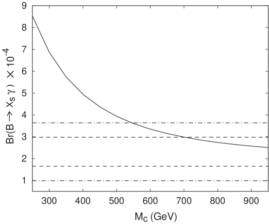
Figure 2: $Br(B\to X_{s}\gamma)$ in Model III. The experimental result at $1\sigma$ (dashed) and $2\sigma$ (dot-dashed) is also given.

If we disregard $R_{b}^{\rm exp}$, then there is no need to enhance $\xi^{D}_{bb}$ and we can take $\lambda_{bb}=1$ in eq. (16). In this case, Model III predicts a $Br(B\to X_{s}\gamma)$ compatible with experiments at the $2\sigma$-level, for $M_{c}\geq 600$ GeV, as we can see in Fig. 2. As soon as $\xi^{D}_{bb}$ is not enhanced anymore, the contribution of the neutral scalars and pseudoscalar is completely negligible. Therefore, both the value of the mixing angle $\alpha$ and of the neutral scalar and pseudoscalar masses ($M_{H}$, $M_{h}$ and $M_{A}$) are irrelevant. In particular, Fig. 2 is obtained for $\alpha=\pi/4$ and values for ($M_{H}$, $M_{h}$, $M_{A}$) resulting from the fit to $\Delta\rho_{0}$, as we will discuss in a while. Due to the qualitative character of our analysis, at this point it sufficies to seek consistency with the experiment at the $2\sigma$-level. Indeed, we took as reference the SM calculation [31], which is already affected by a large uncertainty, and computed only the leading corrections due to the new scalar bosons of Model III, i.e. without considering the complete LO effective hamiltonian analysis. From Fig. 2 we also note that, for $M_{c}\geq 600$ GeV, Model III is difficult to distinguish from the SM (again within $2\sigma$), unless the present SM calculation ($Br(B\to X_{s}\gamma)=(1.9\pm 0.6)\times 10^{-4}$ [31]) is improved [34].

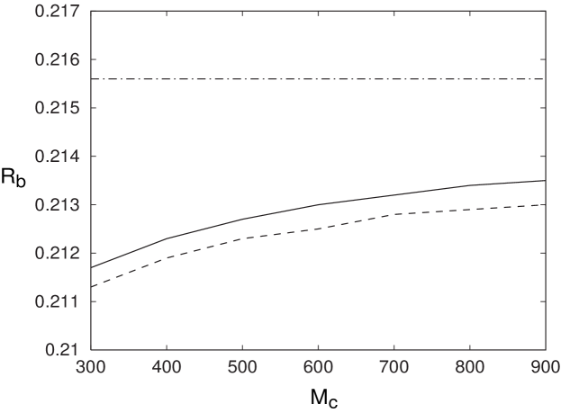
Figure 3: $R_{b}$ in Model III for $\alpha=0$ (solid) and $\alpha=\pi/4$ (dashed). The SM prediction $R_{b}^{\scriptscriptstyle{\rm SM}}=0.2156$ is also given (dot-dashed) for comparison.

With the requirement of a large $M_{c}$ coming from $Br(B\to X_{s}\gamma)$, we need to consider the discussion of $\rho_{0}$ again and modify it accordingly. The charged scalar cannot be the heaviest scalar particle anymore, otherwise $\Delta\rho_{0}^{\scriptscriptstyle{\rm NEW}}$ would be as in eq. (32) and would contradict the present global fit result (see eq. (31)). As already noted in ref. [19] for Model II, there are two other possible scenarios

$$M_{H},M_{h}\leq M_{c}\leq M_{A}\,\,\,\,\,\mbox{and}\,\,\,\,M_{A}\leq M_{c}\leq M_{H},M_{h}$$ (53)

in which $\Delta\rho_{0}^{\scriptscriptstyle{\rm NEW}}$, as given by eq. (29), turns out to be negative, and has in this way the extra advantage of cancelling the effect of the top quark SM contribution (see eq. (26)). We note that none of the previous scenarios would be compatible with an enhanced value of $R_{b}$, because in that case $M_{A}$ and $M_{h}$ would be required to be equal and light (see Section 3).

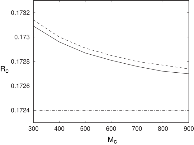
Figure 4: $R_{c}$ in Model III for $\alpha=0$ (solid) and $\alpha=\pi/4$ (dashed). The SM prediction $R_{c}^{\scriptscriptstyle{\rm SM}}=0.1724$ is also given (dot-dashed) for comparison.

From a direct numerical evaluation of $\Delta\rho_{0}^{\scriptscriptstyle{\rm NEW}}$, we find that there may exist many possible sets of mass parameters for which eq. (31) can be satisfied. For instance, let us consider the case in which $M_{H},M_{h}\leq M_{c}\leq M_{A}$. The other case in eq. (53) has been studied too and it gives comparable results. In order to have a small $\Delta\rho_{0}^{\scriptscriptstyle{\rm NEW}}$, it is crucial that $M_{c}$ and $M_{A}$ are not too far apart. One possible optimal set of values for the mass parameters is given by the following ratios: $M_{H}\!=\!0.4\,M_{c}$, $M_{h}\!=\!0.5\,M_{c}$ and $M_{A}\!=\!1.1\,M_{c}$. In this case, the results for $R_{b}$, $R_{c}$ and $R_{b+c}$ are illustrated in Fig. 3 – Fig. 5 respectively. The SM predictions are also plotted for comparison. Clearly, in Model III, $R_{b}$ is less than $R_{b}^{\scriptscriptstyle{\rm SM}}$ and $R_{c}$ is larger than $R_{c}^{\scriptscriptstyle{\rm SM}}$. Thus, if the current experimental trend for $R_{b}^{\rm exp}$ exceeding $R_{b}^{\scriptscriptstyle{\rm SM}}$ persists, Model III will be ruled out.

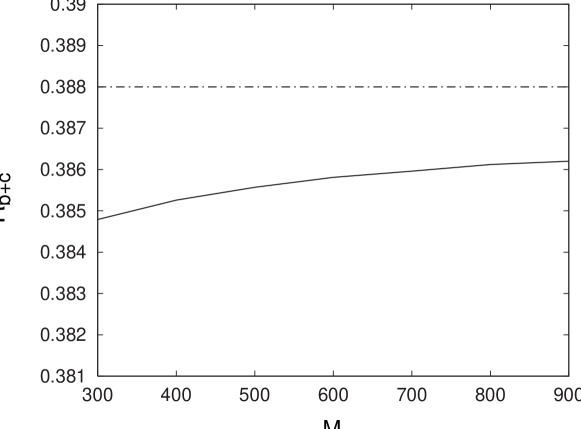
Figure 5: $R_{b+c}$ in Model III (solid) compared to the SM prediction (dot-dashed). The dependence on $\alpha$ is irrelevant.

8 Conclusions

We analyzed the decays $Z\rightarrow b\bar{b}$ and $Z\rightarrow c\bar{c}$ in 2HDM with FCSC, often called Model III. We find that $R_{b}^{\rm exp}$ places severe constraints on this model. It requires that $M_{h}\sim M_{A}\leq 60$ GeV, with significantly enhanced coupling of the neutral scalar and pseudoscalar to $b\bar{b}$. This parameter space of the model cannot be reconciled with constraints from the $\rho$-parameter and $Br(B\rightarrow X_{s}\gamma)$.

Since aspects of the experimental analysis are of some concern, we also examined the model by disregarding $R_{b}^{\rm exp}$ and we give the predictions for $R_{b}$, $R_{c}$ and $R_{b+c}$ in this case. In particular, we find that, if the current trend of $R_{b}^{\rm exp}>R_{b}^{\scriptscriptstyle{\rm SM}}$ persists, then this class of models will be ruled out.

We emphasized the importance of $R_{b+c}$ and $R_{l}$ in our analysis.

In view of the fact that in models with FCSC the rate for $Z\rightarrow c\bar{c}$ receives a correction which grows with $m_{t}^{2}$, we stress that precise measurements of $Z\rightarrow c\bar{c}$ could provide unique constraints on the crucial $tc$-vertex.

Appendix A Feynman rules for Model III

In this appendix we summarize the Feynman rules for Model III which are used in many of the calculations presented in the paper.

A.1 Fermion-Scalar couplings

We present the Feynman rules for the couplings of the scalar fields $H^{1}$ (neutral scalar), $H^{2}$ (neutral pseudoscalar) and $H^{+}$ (charged scalar), to up-type and down-type quarks, as can be derived from the Yukawa Lagrangian of Model III (eqs. (8)-(13)). Following the discussion of Section 2, these are the Feynman rules we need in our calculation of $R_{b}$.

	$\frac{-i}{2\sqrt{2}}\left((\xi_{ij}^{U,D}+\xi_{ij}^{U,D*})+(\xi_{ij}^{U,D}-\xi_{ij}^{U,D*})\gamma_{5}\right)$
	$\frac{1}{2\sqrt{2}}\left((\xi_{ij}^{U,D}-\xi_{ij}^{U,D*})+(\xi_{ij}^{U,D}+\xi_{ij}^{U,D*})\gamma_{5}\right)$
	$\frac{-i}{2}\left(V_{\scriptscriptstyle{\rm CKM}}\!\cdot\!\xi_{ij}^{D}(1+\gamma_{5})-\xi_{ij}^{U}\!\cdot\!V_{\scriptscriptstyle{\rm CKM}}(1-\gamma_{5})\right)$

Although the $\xi_{ij}^{U,D}$ couplings are left complex in the above, in practice, in our calculation we assumed they are real, i.e. $\xi_{ij}^{U,D}\simeq\xi_{ij}^{U,D*}$, as we were not concerned with any phase-dependent effects.

A.2 Gauge boson-Scalar couplings

Here is a list of the Z- and W-boson interactions with Model III scalar fields, useful for the computation of $\Delta\rho_{0}^{\scriptscriptstyle{\rm NEW}}$. We report them in terms of scalar mass eigenstates, $\bar{H}^{0}$, $h^{0}$, $A^{0}$ and $H^{+}$, in order to make contact with the discussion given in Section 4 and with the literature [23, 14]. We always have to remember the relations (see eqs. (2) and (2)) between the scalar mass eigenstates and ($H^{0}$, $H^{1}$, $H^{2}$, $H^{+}$) and use the fact that neither $ZH^{0}H^{1}$ nor $ZH^{0}H^{2}$ couplings are present [23, 14].

	$\frac{g_{\scriptscriptstyle W}}{2c_{\scriptscriptstyle W}}\sin\alpha\,(p_{2}-p_{1})^{\mu}$
	$\frac{g_{\scriptscriptstyle W}}{2c_{\scriptscriptstyle W}}\cos\alpha\,(p_{2}-p_{1})^{\mu}$
	$\frac{ig_{\scriptscriptstyle W}}{2c_{\scriptscriptstyle W}}(1-2s_{\scriptscriptstyle W}^{2})(p_{2}-p_{1})^{\mu}$
	$ie\,(p_{2}-p_{1})^{\mu}$

	$\frac{g_{\scriptscriptstyle W}}{2}(p_{2}-p_{1})^{\mu}$
	$\frac{-ig_{\scriptscriptstyle W}}{2}\cos\alpha\,(p_{2}-p_{1})^{\mu}$
	$\frac{-ig_{\scriptscriptstyle W}}{2}\sin\alpha\,(p_{2}-p_{1})^{\mu}$

Appendix B Calculation of $R_{\ell}$ as a function of $\alpha_{s}$

In this Appendix we will use the value of $\alpha_{s}(M_{Z})$ deduced from physics other than the width for $Z\to{}$hadrons to predict $\Gamma^{\scriptscriptstyle{\rm SM}}(Z\to{}$hadrons) and $R^{\scriptscriptstyle{\rm SM}}_{\ell}$ to $0(\alpha^{2}_{s})$. Mostly, we follow Bernabéu et al. [2], who give expressions for various corrections to $\Gamma(Z\to f\bar{f})$, for both quarks and leptons.

Let us rewrite the expression for the width of $Z\to f\bar{f}$ as

$$\Gamma(Z\to f\bar{f})=\Gamma^{f}_{0}(1+\Delta_{\rm EW}^{f})(1+\Delta_{\rm QCD}^{f})$$ (54)

where $\Gamma^{f}_{0}$ is the tree level expression, in which some effects of the EW corrections have been reabsorbed in the renormalization of the couplings (see conventions adopted in [2]). $\Delta_{\rm EW}^{f}$ includes only corrections which do not depend on $\alpha_{s}$, i.e. pure EW corrections and QED corrections. They are presented in detail in ref. [2] (eqs. (9), (15) and (17), see also references therein) and we will not discuss them here. We give their numerical values [35] in Table 1.

$\nu$	$e,\mu,\tau$	$u,c$	$d,s$	$b$
3.739	2.736	2.200	2.778	-13.848

Table 1: Values of $\Delta_{\rm EW}^{f}$, for different flavors, in units of ($10^{-3}$). They have been evaluated for $m_{t}=176$ GeV and $m_{H}=200$ GeV.

$\Delta_{\rm QCD}^{f}$ represents mostly $\alpha_{s}$-dependent corrections which can be subdivided as

$$\Delta^{f}_{\rm QCD}=\delta_{\rm QCD}+\delta^{f}_{\mu\rm QCD}+\delta^{f}_{t\rm QCD}$$ (55)

We briefly discuss each of them below.

The strong corrections to the basic $V,A$ vertex ($V=\gamma^{\mu}$, $A=\gamma^{\mu}\gamma^{5}$) are flavor-independent and at $O(\alpha_{s}^{2})$ are given by

$$\delta_{\rm QCD}=\frac{\alpha_{s}(M_{Z})}{\pi}+1.41\left(\frac{\alpha_{s}(M_{Z})}{\pi}\right)^{2}$$ (56)

This is the dominant effect amounting to about 3–4% (see Table 2).

$\delta^{f}_{\mu\rm{QCD}}$ represents corrections due to kinematic effects of external masses, including mass-dependent QCD corrections [36, 37]. We decide to include in the same factor also non QCD mass-dependent corrections to the axial vector couplings, in order to make the presentation more compact. Strictly speaking, this correction should be included in $\Delta^{f}_{\rm EW}$. Based on the results given in ref. [36, 37], we deduce [38]

$$\delta^{f}_{\mu\rm{QCD}}=\frac{3\mu^{2}_{f}}{v^{2}_{f}+a^{2}_{f}}\left[-\frac{1}{2}a^{2}_{f}\left(1+\frac{11}{3}\,\frac{\alpha_{s}}{\pi}\right)+v^{2}_{f}\left(\frac{\alpha_{s}}{\pi}\right)\right]$$ (57)

where $\mu^{2}_{f}=4\bar{m}^{2}_{f}(M_{Z})/m^{2}_{Z}$, $\bar{m}_{f}(M_{Z})$ being the running mass at the Z-scale, and

$$v_{e} =-1+4x_{\scriptscriptstyle{\rm W}}\quad,\quad a_{e} =+1$$

$$v_{u} =+1-\frac{8}{3}x_{\scriptscriptstyle{\rm W}}\quad,\quad a_{u} =-1$$ (58)

$$v_{d} =-1+\frac{4}{3}x_{\scriptscriptstyle{\rm W}}\quad,\quad a_{d} =+1$$

Using eq. (2) from ref. [2], we obtain $x_{\scriptscriptstyle{\rm W}}=.2314$ (where $x_{\scriptscriptstyle{\rm W}}=\sin^{2}\!\theta_{\rm W}$). Numerically, $\delta^{b}_{\mu\rm{QCD}}\simeq-5\times 10^{-3}$ and $\delta^{c}_{\mu\rm{QCD}}\sim-0.5\times 10^{-3}$ (see Table 2 for their $\alpha_{s}$-dependence). This kind of correction is also relevant, without $O(\alpha_{s})$ terms, for the $\tau$ lepton, in which case it amounts to $\delta^{\tau}_{\mu}\simeq-2\times 10^{-3}$.

At $O(\alpha^{2}_{s})$ the large mass splitting between the $t$ and $b$ quarks gives rise to a correction, $\delta^{f}_{t{\rm QCD}}$, due to triangular quark loops affecting the axial vector current [37]:

$$\delta^{f}_{t\rm QCD}=-\frac{a_{t}a_{f}}{v^{2}_{f}+a^{2}_{f}}\left(\frac{\alpha_{s}}{\pi}\right)^{2}f(\mu_{t})$$ (59)

where $f(\mu_{t})$ can be written as [37, 2]

$$f(\mu_{t})=\log\frac{4}{\mu_{t}^{2}}-3.083+0.346\frac{1}{\mu_{t}^{2}}+0.211\frac{1}{\mu_{t}^{4}}$$ (60)

For $m_{t}=176$ GeV we use $f(\mu_{t})=-4.374$. Thus, this correction effects $+2/3$ charge-quarks positively and $-1/3$ charge-quarks negatively and for each flavor it is about 0.4-0.5%, as we can read from Table 2.

$\alpha_{s}(M_{Z})$	$\delta_{QCD}$	$\delta^{b}_{\mu\rm{QCD}}$	$\delta^{c}_{\mu\rm{QCD}}$	$\delta^{u}_{t\rm{QCD}}$	$\delta^{d}_{t\rm{QCD}}$
0.105	34.998	-5.417	-0.560	4.260	-3.305
0.110	36.742	-5.179	-0.514	4.676	-3.628
0.115	38.495	-4.938	-0.467	5.111	-3.965
0.120	40.254	-4.695	-0.420	5.565	-4.317
0.125	42.021	-4.450	-0.372	6.038	-4.684

Table 2: Values of different QCD corrections (in units of $10^{-3}$), for different values of $\alpha_{s}(M_{Z})$.

Having identified all the corrections to $\Gamma_{f}\!=\!\Gamma(Z\to f\bar{f})$, for both quarks and leptons, we then consider $R_{\ell}$ and define

$$R_{\ell} = \frac{(\Gamma_{u}+\Gamma_{d}+\Gamma_{s}+\Gamma_{c}+\Gamma_{b})}{\Gamma_{\ell}}$$

$$= \sum_{f=u,d,s,c,b}R^{f}_{\ell,0}\frac{(1+\Delta^{f}_{\rm EW})}{(1+\Delta^{\ell}_{\rm EW}+\delta^{\tau}_{\mu}/3)}(1+\Delta^{f}_{\rm QCD})$$

where $\Gamma_{\ell}=(\Gamma_{e}+\Gamma_{\mu}+\Gamma_{\tau})/3$ and $\Delta^{\ell}_{\rm EW}$ represents the EW corrections common to all the lepton species (see Table 1). We have denoted by $R^{f}_{\ell,0}$ the tree level ratios for each quark species. They are given by

$$R^{u}_{\ell,0} = \frac{\Gamma^{u}_{0}}{\Gamma^{e}_{0}}=3\frac{v^{2}_{u}+a^{2}_{u}}{v^{2}_{e}+a^{2}_{e}}$$

$$R^{d}_{\ell,0} = \frac{\Gamma^{d}_{0}}{\Gamma^{e}_{0}}=3\frac{v^{d}_{d}+a^{2}_{d}}{v^{2}_{e}+a^{2}_{e}}$$ (62)

and for $x_{\scriptscriptstyle{\rm W}}=.2348$ they can be estimated to be $R^{u}_{\ell,0}=3.4209$ and $R^{d}_{\ell,0}=4.4101$.

Finally, $\Delta^{f}_{\rm QCD}$ represents the total QCD corrections for each flavor. They are deduced from the previous discussion and their numerical values are summarized in Table 3, together with $R_{\ell}$, for different values of $\alpha_{s}(M_{Z})$.

Using the values for $\Delta^{f}_{\rm EW}$ given, for each flavor, in Table 1, $R_{\ell}$ can be parametrized as follows ($\alpha_{s}=\alpha_{s}(M_{Z})$)

$$R_{\ell} = R^{u}_{\ell,0}\,(1.000219)\,(2+\Delta^{u}_{\rm QCD}(\alpha_{s})+\Delta^{c}_{\rm QCD}(\alpha_{s}))+$$

$$2R^{d}_{\ell,0}\,(1.000796)\,(1+\Delta^{d,s}_{\rm QCD}(\alpha_{s}))+$$

$$R^{d}_{\ell,0}\,(0.984199)\,(1+\Delta^{b}_{\rm QCD}(\alpha_{s}))$$

from where we deduce the values reported in Table 3.

$\alpha_{s}(M_{Z})$	$\Delta^{u}_{\rm QCD}$	$\Delta^{c}_{\rm QCD}$	$\Delta^{d,s}_{\rm QCD}$	$\Delta^{b}_{\rm QCD}$	$R_{\ell}$
0.105	39.258	38.698	31.693	26.276	20.6715
0.110	41.418	40.904	33.114	27.935	20.7060
0.115	43.606	43.139	34.530	29.592	20.7410
0.120	45.819	45.399	35.937	31.242	20.7759
0.125	48.059	47.678	37.337	32.887	20.8108

Table 3: Values of $R_{l}$ and its QCD corrections (in units of $10^{-3}$) as functions of $\alpha_{s}(M_{Z})$.

References

- [1] Results presented at the International Europhysics Conference on High Energy Physics, Brussels, 1995 and at the 17th International Symposium on Lepton-Photon Interactions, Beijing, China, 1995. See also: LEP Electroweak Working Group Report 95-02.
- [2] J. Bernabéu, A. Pich and A. Santamaria, Nucl. Phys. B363, 326 (1991).
- [3] Here is an illustrative sample of some of the existing studies: A. Denner, R.J. Guth, W. Hollik and J.H. Kühn, Zeit. Phys. C51, 695 (1991); A.K. Grant, Phys. Rev. D51, 207 (1995); J.T. Liu and D. Ng, Phys. Lett. B342, 262 (1995); E. Ma and D. Ng, Phys. Rev. D53, 255 (1996); J.D. Wells, C. Kolda and G.L. Kane, Phys. Lett. B338, 219 (1994); J.D. Wells and G.L. Kane, preprint hep-ph/9510372; G. Bhattacharyya, G. Branco and W.-S. Hou, hep-ph/9512239; T. Rizzo, talk given at the Heavy Flavor Symposium, Haifa (Israel), Dec. 1995; P. Chiappetta, J. Layssac, F.M. Renard and C. Verzegnassi, hep-ph/9601306; G. Altarelli, N. di Bartolomeo, F. Feruglio, R. Gatto and M.L. Mangano, hep-ph/9601324.
- [4] T.P. Cheng and M. Sher, Phys. Rev. D35, 3484 (1987); D44, 1461 (1991); see also Ref. [5].
- [5] A. Antaramian, L.J. Hall, and A. Rasin, Phys. Rev. Lett. 69, 1871 (1992).
- [6] L.J. Hall and S. Weinberg, Phys. Rev. D48, R979 (1993).
- [7] W.S. Hou, Phys. Lett. B296, 179 (1992); D. Chang, W.S. Hou and W.Y. Keung; Phys. Rev. D48, 217 (1993).
- [8] M. Luke and M.J. Savage, Phys. Lett. B307, 387 (1993); M.J. Savage, Phys. Lett. B266, 135 (1991).
- [9] D. Atwood, L. Reina and A. Soni, Phys. Rev. D53, R1199 (1996);
- [10] D. Atwood, L. Reina and A. Soni, Phys. Rev. Lett. 75, 3800 (1995).
- [11] S. Glashow and S. Weinberg, Phys. Rev. D15, 1958 (1977).
- [12] For a review see J. Gunion, H. Haber, G. Kane, and S. Dawson, The Higgs Hunter’s Guide, (Addison-Wesley, New York, 1990).
- [13] T. Han, R.D. Peccei and X. Zhang, Nucl. Phys. B454, 527 (1995).
- [14] C.D. Froggatt, R.G.Moorhouse and I.G. Knowles, Nucl. Phys. B386, 63 (1992).
- [15] A detailed phenomenological analysis [16] shows that for the first family one needs in eq. (16) in order to satisfy the bounds from - and - mixing over a large region of the parameter space of Model III. Therefore, in this work we will assume that the FC couplings which involves the first family are negligibly small.
- [16] D. Atwood, L. Reina and A. Soni, in preparation.
- [17] In our calculation all the quarks except the top quark are taken to be massless, keeping only in the couplings as in eq. (16) and in the determination of some corrections to , when they become relevant to the degree of accuracy that we seek.
- [18] A. Denner, R.J. Guth, W. Hollik and J.H. Kühn, Zeit. Phys. C51, 695 (1991).
- [19] A.K. Grant, Phys. Rev. D51, 207 (1995).
- [20] Review of Particles Properties, Phys. Rev. D50, 1173 (1994).
- [21] In obtaining the result in eq. (24) we had calculated both and in Model III. Therefore the corresponding experimental number differs a little bit from that in eq. (2) which is determined by holding fixed to its experimental value (see ref. [1]).
- [22] P. Langacker, hep-ph/9412361, to be published in “Precision Tests of the Standard Electroweak Model”, ed. by P. Langacker.
- [23] S. Bertolini, Nucl. Phys. B272, 77 (1986).
- [24] F. Abe et al., [CDF], Phys. Rev. Lett. 74, 2626 (1995); S. Abachi et al., [], Phys. Rev. Lett. 74, 2632 (1995).
- [25] R. Ammar et al., (CLEO), Phys. Rev. Lett. 71, 674 (1993); M.S. Alam et al. [CLEO], Phys. Rev. Lett. 74, 2885 (1995).
- [26] Note that we are considering the case , as required by the best fit of .
- [27] B. Grinstein, R. Springer, and M. Wise, Phys. Lett. B202, 132 (1988); Nucl. Phys. B339, 269 (1990); R. Grigjanis, P.J. O’Donnel, M. Sutherland and H. Navelet, Phys. Lett. B213, 355 (1988); Phys. Lett. B223, 239 (1989); Phys. Lett. B237, 252 (1990); G. Cella, G. Curci, G. Ricciardi and A. Viceré, Phys. Lett. B248, 181 (1990), Phys. Lett. B325, 227 (1994); M. Misiak, Nuc. Phys B393, 23 (1993); K. Adel and Y.P. Yao, Phys. Rev. D49, 4945 (1994).
- [28] M. Ciuchini, E. Franco, G. Martinelli, L. Reina and L. Silvestrini, Phys. Lett. B316, 127 (1993); Nucl. Phys. B421, 41 (1994).
- [29] A.J. Buras, M. Misiak, M. Münz and S. Pokorski, Nucl. Phys. B424, 137 (1994).
- [30] We use the same normalization as in ref. [29], in order to check our result against the discussion of the problem in Model II, as given in that paper.
- [31] M. Ciuchini, E. Franco, G. Martinelli, L. Reina and L. Silvestrini, Phys. Lett. B344, 137 (1994).
- [32] A.X. El-Khadra, G. Hockney, A. Kronfeld and P. Mackenzie, Phys. Rev. Lett. 69, 729 (1992); C.T.H. Davies, K.Hornbostel, G.P. Lepage, A. Lidsey, J. Shigemitsu and J. Sloan, Phys. Lett. B345, 42 (1995).
- [33] In this regard see the analysis by M. Shifman (hep-ph/9511469), using the Z-line shape (rather than ) and the value of advocated by M. Voloshin in Int. J. Mod. Phys. A10, 2865 (1995). It is interesting that both these observables (Z-line shape and ) lead to similar conclusions when is used.
- [34] The theoretical prediction of from ref. [31] includes some NLO QCD corrections and the result could change in the future by a complete NLO analysis. We could have used in our analysis the fully consistent LO result for , which is a little higher (see ref. [31, 29]), but this would not modify the qualitative results that we are giving.
- [35] depend very weakly on . The numerical values quoted in Table 1 are for GeV.
- [36] K.G. Chetyrkin and J.H. Kühn, Phys. Lett. B248, 359 (1990).
- [37] B.A. Kniehl and J.H. Kühn, Nucl. Phys. B329, 547 (1990).
- [38] Note that our eq. (57) differs from eq. (19) of ref. [2]. We derive eq. (57) from ref. [36], where the results of ref. [37] are improved by absorbing large through the use of the running mass . Using eqs. (2) and (4) of ref. [36] and substituting the on-shell mass with the mass as in eq. (9) therein, we confirm their result in eq. (14). Thus we arrive to our eq. (57).