CERN-TH/96-13

INR-913/96

hep-ph/9603208

March 1, 1996

ELECTROWEAK BARYON NUMBER NON-CONSERVATION IN THE EARLY UNIVERSE AND IN HIGH ENERGY COLLISIONS

V. A. Rubakov^a, and M. E. Shaposhnikov^b,a,
a Institute for Nuclear Research of the Russian Academy of Sciences,
60-th October Anniversary Prospect 7a, Moscow 117312, Russia
^bTheory Division, CERN, CH-1211 Geneva 23, Switzerland

Abstract

We review recent progress in the study of the anomalous baryon number non-conservation at high temperatures and in high energy collisions. Recent results on high temperature phase transitions are described, and applications to electroweak baryogenesis are considered. The current status of the problem of electroweak instanton-like processes at high energies is outlined. This paper is written on the occasion of Sakharov’s 75th anniversary and will appear in the memorial volume of Uspekhi (Usp. Fiz. Nauk, volume 166, No 5, May 1996).

CERN-TH/96-13
INR-913/96
March 1, 1996

1 Introduction

In his famous paper [1] Sakharov discussed for the first time the possibility of explaining the charge asymmetry of the Universe in terms of particle theory. The paper was submitted to JETP Letters in September 1966, two years after the discovery of CP-violation in $K^{0}$ decays [2] and one year after the microwave black-body radiation, predicted by the Big Bang theory [3], was found experimentally [4]. To explain baryon asymmetry, Sakharov proposed an approximate character for the baryon conservation law, i.e., baryon number non-conservation and proton decay. Three years later Kuzmin published a paper [5] where a different model leading to the baryon asymmetry was constructed. One of its consequences was another process with B non-conservation, namely, neutron-antineutron oscillations. Since that time the idea that baryon number may not be exactly conserved in Nature has been elaborated upon considerably, both in the context of the generation of the baryon asymmetry of the Universe [6, 7, 8, 9, 10, 11] (for reviews see refs. [12, 13, 14]) and because of theoretical developments that have lead to a unified picture of fundamental interactions. In the mid–70’s, grand unified theories with inherent violation of baryon number were put forward [15, 16, 17, 18, 19]. Almost at the same time it was realized [20, 21] that non-perturbative effects related to instantons [22] and the complex structure of gauge theory vacuum [20, 23, 24] lead to the non-conservation of baryon number even in the electroweak theory; it has been understood later [25] that similar effects are relevant for the baryon asymmetry.

In his paper [1] Sakharov writes: “According to our hypothesis, the occurrence of C asymmetry is the consequence of violation of CP invariance in the nonstationary expansion of the hot Universe during the superdense stage, as manifest in the difference between the partial probabilities of the charge-conjugate reactions.” Today, this short extract is usually dubbed as three necessary Sakharov’s conditions for baryon asymmetry generation from the initial charge symmetric state in the hot Universe, namely:
(i) Baryon number non-conservation.
(ii) C and CP violation.
(iii) Deviations from thermal equilibrium.
All three conditions are easily understood.

(i) If baryon number were conserved, and the initial baryonic charge of the Universe were zero, the Universe today would be symmetric, rather than asymmetric . The statement of the necessity of the baryon number non-conservation was quite revolutionary at that time. Today it is very natural theoretically; still, lacking positive results from experiments searching for B non-conservation, the baryon asymmetry of the Universe is a unique observational evidence in favour of it.

(ii) If C or CP were conserved, then the rate of reactions with particles would be the same as the rate of reactions with antiparticles. If the initial state of the Universe was C- or CP- symmetric, then no charge asymmetry could develop from it . In more formal language, this follows from the fact that if the initial density matrix of the system $\rho_{0}$ commutes with C- or CP-operations, and the Hamiltonian of the system is C- or CP-invariant, then at any time the density matrix $\rho(t)$ is C- or CP-invariant, so that the average of any C- or CP-odd operator is zero.

(iii) Thermal equilibrium means that the system is stationary (no time dependence at all). Hence, if the initial baryon number is zero, then it is zero forever.

Clearly, the issue of the baryon asymmetry generation requires the development of many different areas of theoretical physics, such as model building, study of perturbative and non-perturbative effects leading to B-violation, finite temperature field theory and non-equilibrium statistical mechanics, theory of phase transitions.

In this paper we do not aim to give a complete review of various theories of baryogenesis proposed so far. The reader may consult with a number of reviews on this subject [12, 13, 14, 26, 27, 28, 29, 30]. Instead, we pick up a specific non-perturbative mechanism of the baryon number non-conservation, associated with triangle anomaly. The choice of this mechanism is explained, partially, by the authors’ personal taste. In addition, anomalous fermion number non-conservation is a general phenomenon for theories with chiral fermions, and is present, e.g., in the standard model of electroweak interactions. This mechanism, being operative at high temperatures, may lead to the baryogenesis at the electroweak scale.

The possibility that baryon asymmetry may be due to physics which is probed at accessible energies has attracted a lot of attention recently and serves as a powerful motivation for the development of high temperature field theory, theory of phase transitions, non-equilibrium statistical mechanics.

The fact that baryon number is rapidly violated at high temperatures [25] (for earlir discussion see [31, 8, 32]) and under other extremal conditions [33, 34, 35, 36, 37, 38] naturally leads one to enquire whether electroweak baryon number non-conservations occurs at high enough rate in collisions of energetic particles. This problem has attracted considerable interest in recent years, after the first — and encouraging at the time — quantitative results were obtained [39, 40]. In spite of remarkable theoretical developments, this problem is still not completely solved; existing results indicate that the electroweak baryon number violating processes occur at unobservable rates even at very high energies.

The paper is organized as follows. In Section 2 we provide the necessary background and discuss the mechanism of anomalous non-conservation of fermionic quantum numbers together with relevant bosonic classical solutions (instantons and sphalerons). Section 3 contains preliminary discussion of the role of baryon number violating electroweak processes in early Universe. The fermion number non-conservation at high temperatures is considered in Section 4. In Section 5 we present recent developments in the theory of high temperature phase transitions. In Section 6 we briefly address the question of survival of the primordial baryon asymmetry. The discussion of various electroweak baryogenesis mechanisms is contained in Section 7. We turn to electroweak baryon number non-conservation in particle collisions in Section 8. Section 9 contains concluding remarks.

2 Basics of anomalous non-conservation of fermion quantum numbers

Let us discuss non-perturbative non-conservation of fermion quantum numbers in the context of a model with the gauge group $SU(2)$ and the massless left-handed fermionic doublets $\psi_{L}^{(i)}$, $i=1,\dots,n_{L}$. The absence of global anomaly [41] requires that $n_{L}$ is even. We also add a Higgs doublet $\phi$ that breaks the $SU(2)$ symmetry completely. Then this theory is a simplified version of the electroweak sector of the minimal standard model. All relevant features of the standard model are present in this simplified theory; later on we shall comment on minor complications due to $U(1)_{Y}$ gauge symmetry, right-handed fermions and Yukawa interactions leading to fermion masses. One may regard the simplified theory as the standard model in the approximation where $\sin\theta_{W}$ and all fermion masses are set to zero; for three families of quarks and leptons one has $n_{L}=12$ and

$$\psi_{L}^{(i)}=\{q_{L}^{f,\alpha},l_{L}^{f}\},$$ (2.1)

where $f=1,2,3$ is the family index and $\alpha=1,2,3$ labels the colour of quarks.

At the classical level, there exist $n_{L}$ conserved global $U(1)$ currents,

$$J^{(i)}_{\mu}=\bar{\psi}^{(i)}_{L}\gamma^{\mu}\psi^{(i)}_{L},$$

which correspond to the conservation of the number of each fermionic species. At the quantum level these currents are no longer conserved due to the triangle anomaly [42, 43, 44]

$$\partial_{\mu}J_{\mu}^{(i)}=\frac{1}{32\pi^{2}}\mbox{Tr}\left(F_{\mu\nu}\tilde{F}_{\mu\nu}\right).$$ (2.2)

Therefore, one expects that fermion numbers $N_{F}^{(i)}=\int~{}d^{3}x~{}J^{(i)}_{0}$ are not conserved in any process where the gauge field evolves in such a way that

$$N[A]=\frac{1}{32\pi^{2}}\int~{}d^{4}x~{}\mbox{Tr}F_{\mu\nu}\tilde{F}_{\mu\nu}\neq 0.$$ (2.3)

Namely,

$$\Delta N_{F}^{(i)}=N[A],~{}~{}~{}~{}i=1,\dots,n_{L}.$$ (2.4)

It is clear from eq. (2.3) that in weakly coupled theories, one has to deal with strong fields: the field $F_{\mu\nu}=\frac{g}{2i}\tau^{a}F^{a}_{\mu\nu}$ should be of order $1$, and $A_{\mu}^{a}=O(g^{-1})$. So, it is natural that the (semi)classical treatment of bosonic fields is often reliable.

Equation (2.4) may be viewed as the selection rule: the number of fermions changes by the same amount for every species. In terms of the assignment (2.1) it implies, in particular,

$$\Delta N_{e}=\Delta N_{\mu}=\Delta N_{\tau}=N[A],$$

$$\Delta B=\frac{1}{3}\cdot 3\cdot 3\cdot N[A],$$ (2.5)

where the factor $1/3$ comes from the baryon number of a quark, while the factor $3\cdot 3$ is due to colour and number of generations. So, the amounts of non-conservation of baryon and lepton numbers are related:

$$\Delta N_{e}=\Delta N_{\mu}=\Delta N_{\tau}=\frac{1}{3}\Delta B,$$

$(B-L)$ is conserved while $(B+L)$ is violated.

The analysis of gauge field configurations with the non-zero topological number (2.3) is conveniently performed in the gauge

$$A_{0}=0.$$

In this gauge, there exists a discrete set of classical vacua, i.e. pure gauge configurations

$$A_{i}=\omega\partial_{i}\omega^{-1},$$

$$\phi=\omega\phi_{0},$$

where $\phi_{0}=(0,v/\sqrt{2})$ is the Higgs field in the trivial vacuum. The gauge functions $\omega$ depend only on spatial coordinates $\omega=\omega({\bf x})$ and are characterized by an integer:

$$n[\omega]=-\frac{1}{24\pi^{2}}\int~{}d^{3}x~{}\epsilon^{ijk}\mbox{Tr}(\omega\partial_{i}\omega^{-1}\cdot\omega\partial_{j}\omega^{-1}\cdot\omega\partial_{k}\omega^{-1}).$$

The vacua with different $n[\omega]$ cannot be continuously deformed into each other without generating non-vacuum gauge fields, so these vacua are separated by a potential barrier. Therefore, the gauge–Higgs system is similar to a particle in periodic potential, as shown in fig. 1. An explicit construction of the minimum energy path connecting the neighboring vacua was carried out in ref. [45], and the fermion sea contribution to this path was evaluated in ref. [46].

The topological number density entering eq. (2.3) is a total derivative,

$$\frac{1}{32\pi^{2}}\mbox{Tr}(F_{\mu\nu}\tilde{F}_{\mu\nu})=\partial_{\mu}K_{\mu},$$

where

$$K_{\mu}=\epsilon^{\mu\nu\lambda\rho}\mbox{Tr}\left(F_{\nu\lambda}A_{\rho}-\frac{2}{3}A_{\nu}A_{\lambda}A_{\rho}\right).$$

If one is interested in vacuum–vacuum transitions, then

$$N[A]=\int~{}d^{3}xdt~{}\partial_{\mu}K_{\mu}=\left[\int~{}d^{3}x~{}K_{0}\right]^{t=+\infty}_{t=-\infty}$$

$${}~{}~{}~{}~{}~{}~{}~{}~{}~{}~{}~{}~{}~{}~{}~{}~{}~{}~{}=n[\omega_{t=+\infty}]-n[\omega_{t=-\infty}].$$

So, the topological number of the gauge field is non-zero for transitions between the distinct vacua.

At zero energies and temperatures, the transition between vacua with different $n[\omega]$ is a tunnelling event which is described by instantons [22] (constrained instantons in theories with the Higgs mechanism [47]). In pure Yang–Mills theory an instanton is the solution to the Euclidean field equations which is an absolute minimum of the Euclidean action in the sector $N[A]=1$. Properties of instantons are reviewed in ref. [48]. The instanton field, up to gauge transformations, is

$$A^{a}_{\mu}=\frac{1}{g}\eta_{\mu\nu a}\frac{2x^{\nu}}{x^{2}+\rho^{2}},$$ (2.6)

where $\eta_{\mu\nu a}$ are the ’t Hooft symbols, and $\rho$ is an arbitrary scale to be integrated over. The instanton action is

$$S_{inst}=\frac{8\pi^{2}}{g^{2}}$$

and the tunnelling amplitude is proportional to

$$A_{inst}\propto\mbox{e}^{-S_{inst}}.$$ (2.7)

In the electroweak theory, the tunneling probability is unobservably small,

$$\sigma_{inst}\propto\exp\left(-\frac{4\pi}{\alpha_{W}}\right)\sim 10^{-170},$$ (2.8)

where

$$\alpha_{W}=\frac{g^{2}}{4\pi}=\frac{\alpha}{\sin^{2}\theta_{W}}=\frac{1}{29}.$$

In theories with the Higgs mechanism there appears a slight complication. There are no solutions to Euclidean field equations, i.e. no exact minima of the Euclidean action in sectors with $N[A]\neq 0$. The reason is that the action for configurations like (2.6), with appropriate Higgs field, depends on the instanton size $\rho$ and decreases as $\rho$ tends to zero. To evaluate the functional integral in that case one introduces a constraint that fixes the size of the configuration [47], then minimizes the action under this constraint and finally integrates over $\rho$. The outcome of this procedure is as follows. The instanton contribution into the functional integral becomes [21, 47]

$$\int~{}d^{4}x_{0}~{}\frac{d\rho}{\rho^{5}}~{}\mu(\rho)\exp\left(-\frac{8\pi^{2}}{g^{2}}-\pi^{2}v^{2}\rho^{2}\right),$$ (2.9)

where $x_{0}$ is the instanton position and $\mu(\rho)$ is a function of $g$ and $\rho$ that varies relatively slowly. The integral (2.9) is saturated at $\rho\mathrel{\raisebox{-2.36806pt}{\hbox to0.0pt{$\sim$\hss}}\raisebox{1.72218pt}{$<$}}v^{-1}$, so that the size of the constrained instantons is smaller than the inverse $W$-boson mass $m_{W}=gv/2$. The constrained instanton configuration is conveniently described in the singular gauge where the original pure Yang–Mills instanton has the form

$$A^{a}_{\mu}=\frac{1}{g}\bar{\eta}_{\mu\nu a}\frac{2\rho^{2}x^{\nu}}{x^{2}(x^{2}+\rho^{2})}.$$ (2.10)

The constrained instanton is given by eq. (2.10) at $x\ll m_{W}^{-1}$, and exponentially decays at large $x$,

$$A^{inst}\propto\mbox{e}^{-m_{W}|x|}.$$

Clearly, the tunnelling rate is still suppressed by the exponential factor (2.8).

In this paper we discuss processes at high temperatures or energies. The relevant energy scale is set by the height of the barrier between different vacua as sketched in fig. 1. This height is determined by the static saddle point solution to the Yang–Mills–Higgs equations, the sphaleron [49, 32]. This solution was found previously in refs. [50, 51, 52, 53], but its relevance to topology was realized only in ref. [32]. By simple scaling one obtains that the static energy of the sphaleron solution in our simplified model, which is equal to the height of the barrier at zero temperature, is

$$E_{sph}=\frac{2m_{W}}{\alpha_{W}}B\left(\frac{m_{H}}{m_{W}}\right),$$ (2.11)

where $m_{H}$ is the mass of the Higgs boson. The function $B(m_{H}/m_{W})$ has been evaluated numerically [32]; it varies from 1.56 to 2.72 as $m_{H}/m_{W}$ varies from zero to infinity . So, the height of the barrier in the electroweak theory is of order 10 TeV.

At energies above $E_{sph}$ the system can in principle evolve from a neighbourhood of one vacuum to another in a classical way, without tunnelling ; as outlined above, this classical process will lead to non-conservation of baryon and lepton numbers. Clearly, having enough energy is a necessary, but not a sufficient condition for the absence of exponential suppression of the baryon and lepton number violation rates. Whether the exponential suppression actually disappears or not is a matter of complicated dynamics which is one of the main subjects of this paper.

There are at least two possible ways to see that fermion quantum numbers are indeed violated in instanton-like processes. One of them [20, 21] makes use of zero fermion modes in Euclidean background fields with $N[A]\neq 0$. This approach is reviewed in ref. [48] and its Minkowskian counterpart is considered in ref. [59]. A more intuitive way [60, 59] is related to the phenomenon of level crossing, which is as follows. Consider left-handed fermions in the background field ${\bf A}({\bf x},t)$ which changes in time from one vacuum at $t=-\infty$ to another vacuum at $t=+\infty$ (we again use the gauge $A_{0}=0$). At each time $t$ one can evaluate the fermionic spectrum, i.e. the set of eigenvalues of the Dirac Hamiltonian in the static background ${\bf A}({\bf x},t)$ where $t$ is viewed as a parameter. The spectrum varies with $t$; some levels cross zero from below and some cross zero from above. The relevant quantity is the net change of the number of positive energy levels, which is the difference between the total number of levels that cross zero from above and from below in the course of the entire evolution from $t=-\infty$ to $t=+\infty$. A general mathematical theorem [61] says that this difference is related to the topological number of the gauge field,

$$N_{+}-N_{-}=n[\omega_{t=+\infty}]-n[\omega_{t=-\infty}]=N[A].$$ (2.12)

Recall now that at vacuum values of ${\bf A}$, the ground state of the fermionic system has all negative energy levels filled and all positive energy levels empty. A real fermion corresponds to filled positive energy level and antifermion is an unoccupied negative energy level. As the energy levels cross zero, the number of real fermions changes, and the net change in the fermion number of each left-handed doublet is

$$\Delta N_{F}^{(i)}=N_{+}-N_{-}.$$

Combining this relation with eq.(2.12) we see that the fermion number is not conserved indeed, and the amount of non-conservation is in perfect agreement with the anomaly relation, eq. (2.4).

Although the above discussion was for massless fermions, the results remain valid for the standard electroweak theory where fermions acquire masses via the Yukawa coupling to the Higgs field [62, 63, 64]. Indeed, the triangle anomaly for baryon and lepton currents remains valid in the standard model, so that relation (2.5) must hold. The counting of fermion zero modes in the instanton background confirms this expectation [62, 64, 65]. Also, the level crossing phenomenon has been explicitly found in theories of this type [66, 67, 65]. So, the complications due to right-handed fermions and fermion masses do not change the picture of baryon and lepton number non-conservation.

Finally, the presence of $U(1)_{Y}$ gauge symmetry in the standard model does not modify the analysis to any considerable extent either. There are no instantons of the $U(1)_{Y}$ gauge field, while the effect of the $U(1)_{Y}$ interactions on the measure $\mu(\rho)$ for $SU(2)$ instantons in eq.(2.9) is tiny. Also, the energy of the $SU(2)$ sphaleron is still given by eq.(2.11) where the factor $B$ depends also on $\sin^{2}\theta_{W}$. For the actual value $\sin^{2}\theta_{W}=0.23$, the deviation of $B$ from its $SU(2)$ values is numerically small [32, 68, 69].

3 Baryon asymmetry: preliminaries

In this section we qualitatively discuss the issues relevant to the main topic of this review – electroweak baryon number non-conservation at high temperatures and generation of the baryon asymmetry of the Universe. These issues will be considered in much more detail in the following sections, so this section may be regarded as a guide for a reader not familiar with the subject. Most of what is said in this section should not be taken too literally: we will somewhat oversimplify the picture of the electroweak physics in the early Universe and hence will use fairly loose terms.

In hot Big Bang cosmology, there is an epoch of particular interest from the point of view of the electroweak physics. This is the epoch of the electroweak phase transition, the relevant temperatures being of the order of a few hundred GeV [70, 71, 72, 73]. Before the phase transition (high temperatures), the Higgs expectation value is zero, while after the phase transition the Higgs field develops a non-vanishing expectation value. The critical temperature $T_{c}$ depends on the parameters of the electroweak theory; in the Minimal Standard Model (MSM) the only grossly unknown parameter is the mass of the Higgs boson, $m_{H}$. In extensions of the MSM, there are more parameters that determine $T_{c}$.

At sufficiently small $m_{H}$ in MSM, the phase transition is of the first order, while at large $m_{H}$ the exact nature of the phase transition is still not clear: it may be weakly first order, second order or smooth cross-over. It is important that the masses of $W$- and $Z$-bosons immediately after the phase transition, $m_{W}(T_{c})$ and $m_{Z}(T_{c})$, are smaller than their zero temperature values; the precise behaviour of $m_{W}(T)$ and $m_{Z}(T)$ again depends on the parameters of the model (on $m_{H}$ in the MSM). Generally speaking, the stronger the first order phase transition, the larger $m_{W}(T_{c})$ and $m_{Z}(T_{c})$. The electroweak phase transition is considered in more detail in section 5.

Let us now turn to the rate of the electroweak baryon number non-conservation at high temperatures. While at zero temperatures the $B$ non-conservation comes from tunnelling and is unobservably small because of the tunnelling exponent, it may proceed at high temperatures via thermal jumps over the barrier shown in fig. 1 [25]. At temperatures below the critical one, $T<T_{c}$, the probability to find the system at the saddle point separating the topologically distinct vacua is still suppressed, but now by the Boltzmann factor,

$$\Gamma\propto\exp\left(-\frac{E_{sph}(T)}{T}\right),$$ (3.1)

where

$$E_{sph}(T)=\frac{2m_{W}(T)}{\alpha_{W}}B\left(\frac{m_{H}}{m_{W}}\right)$$

is the free energy of the sphaleron. Once the system jumps up to the saddle point (i.e. once the sphaleron is thermally created), the system may roll down to the neighbouring vacuum, and the baryon and lepton numbers may be violated. Therefore, the factor (3.1) is also the suppression factor for the rate of the electroweak baryon number non-conservation at $T<T_{c}$.

At $T>T_{c}$, the exponential suppression of the baryon number non-conserving transitions is absent. The power-counting estimate of the rate per unit time per unit volume in the unbroken phase is then [74, 75]

$$\Gamma=\mbox{const}\cdot\left(\alpha_{W}T\right)^{4},$$ (3.2)

where the constant is of order $1$. The rate of the electroweak $B$ non-conservation is considered in detail in section 4.

The rates (3.1) and (3.2) are to be compared with the rate of expansion of the Universe,

$$\frac{1}{t_{U}}=\mbox{const}\cdot\left(\frac{T}{M_{Pl}}\right)T,$$

where the constant is of order $10^{-1}$. Clearly, in the unbroken phase the $B$ non-conservation rate is much higher than the expansion rate in a wide interval of temperatures, $T_{c}<T<0.1\cdot M_{Pl}\alpha_{W}^{4}\sim 10^{12}$ GeV. Therefore, the electroweak $B$ non-conserving reactions are fast at these temperatures. After the phase transition the situation is more subtle: the rate of $B$ non-conservation exceeds the expansion rate if the phase transition is weakly first order ($m_{W}(T_{c})$ is small) or second order or of the cross-over type; on the other hand, the rate of $B$-violating processes is much lower than the expansion rate if the phase transition is strongly first order ($m_{W}(T_{c})$ is large enough). The electroweak $B$ non-conservation switches off immediately after the phase transition if $\frac{E_{sph}(T_{c})}{T_{c}}>45$ (see sections 6 and 7) and operates after the phase transition in the opposite case. This inequality is not satisfied in the MSM (section 7) with $m_{top}=175$ GeV and experimentally allowed Higgs mass $m_{H}>65$ GeV. So, the $B$-violating reactions are fast after the phase transition in the MSM.

In the extensions of the MSM, the properties of the phase transition are determined by more parameters than just the zero temperature Higgs boson mass. So, for some region of the parameter space, the electroweak $B$ non-conservation is negligible after the phase transition.

Clearly, the above observations are directly relevant to the problem of the generation of the baryon asymmetry of the Universe whose quantitative measure is the dimensionless ratio of the baryon number density to entropy density,

$$\Delta_{B}=\frac{B}{s}.$$

This quantity is almost constant during the expansion of the Universe at the stages when baryon number is conserved, and its present value is

$$\Delta_{B}=(4-6)\times 10^{-11}.$$

Several possibilities to generate the baryon asymmetry are discussed in the literature, which differ by the characteristic temperature at which the asymmetry is produced.

(i) Temperature of grand unification, $T\sim 10^{15}-10^{16}$ GeV.

A viable possibility is that the observed baryon asymmetry is generated by baryon number violating interactions of grand unified theories. The effect of the electroweak processes is basically that $(B+L)$, generated at grand unified temperatures, is washed out at some later time (recall that $(B-L)$ is conserved by anomalous electroweak processes). The asymmetry may survive from the grand unification epoch only if a large $(B-L)$ asymmetry is generated at $T\sim 10^{15}-10^{16}$ GeV, and there are no strong lepton number violating interactions at intermediate temperatures, $100$ GeV $<T<10^{12}$ GeV (otherwise all fermionic quantum numbers are violated at these temperatures, and the baryon asymmetry is washed out). The first requirement points to non-standard, $(B-L)$ violating modes of proton decay, though this indication is not strong. We discuss in section 6 some issues related to this scenario of baryogenesis.

(ii) Intermediate temperatures, $1$ TeV $\ll T\ll 10^{15}$ GeV.

An interesting possibility is that there exist lepton number violating interactions at intermediate scales, and these interactions generate a lepton asymmetry of the Universe at intermediate temperatures. Then this lepton asymmetry is partially reprocessed into baryon asymmetry by anomalous electroweak interactions [76]. Possible manifestations of this scenario are Majorana neutrino masses (which actually may be helpful from the point of view of solar neutrino experiments, for a review see, e.g., ref. [77]) and/or lepton number violating processes like $\mu\to e\gamma$, $\mu\to eee$ and $\mu$-$e$ conversion. A more detailed discussion of this possibility, together with the analysis of concrete models, can be found in refs. [78, 79, 80, 81, 82].

Another mechanism able to generate the baryon asymmetry at intermediate temperatures [83] deals with coherent production of scalar fields carrying baryon number. At a later stage the “scalar” baryon number stored in scalar fields is transferred into an ordinary one. The most recent consideration of this interesting possibility in the framework of the sypersymmetric standard model can be found in ref. [84].

(iii) Electroweak temperatures, $T\sim\mbox{(a~{}few)}\times 100$ GeV.

The remaining possibility is that the observed baryon asymmetry is generated by anomalous electroweak interactions themselves. Since the Universe expands slowly during the electroweak epoch, a considerable departure from equilibrium (the third Sakharov condition) is possible only from the first order phase transition. Indeed, this transition, which proceeds through the nucleation, expansion and collisions of the bubbles of the new phase, is quite a violent phenomenon. The dynamical aspects of the first order phase transitions in the Universe are considered in section 5.

A necessary condition for the electroweak baryogenesis is that the baryon asymmetry created during the electroweak phase transition should not be washed out after the phase transition completes. In other words, the rate of the electroweak $B$-violating transitions has to be negligible immediately after the phase transition. As outlined above, and discussed in detail in section 7, the latter requirement is not fulfilled in the Minimal Standard Model, so the electroweak baryogenesis is only possible in extensions of the MSM. Extending the minimal model is useful in yet another respect: it generally provides extra sources of CP violation beyond the Kobayashi–Maskawa mechanism, so that the second Sakharov condition is satisfied more easily . The phenomenological consequences of these extra sources of CP violation are electric dipole moments of neutron and electron [85, 86], whose values are expected, on the basis of the considerations of baryogenesis [87], to be close to existing experimental limits.

Several specific mechanisms of electroweak baryogenesis are outlined in section 7. The outcome is that the observed baryon asymmetry may naturally be explained within extended versions of the Standard Model. This result is particularly fascinating as the physics involved will be probed at LEP-II and the LHC relatively soon. Naturally, most of our review is devoted to the topics related to the electroweak baryogenesis.

4 Sphaleron rate at finite temperatures

In this section we attempt to describe the present situation with the computation of the rate of fermion number non-conservation at high temperatures. We shall try to separate the exact results from (plausible) assumptions. We begin with the qualitative discussion of the rate and derive the Van’t Hoff–Arrhenius type formulae for the rate, valid at sufficiently low temperatures. Then we derive an exact real-time Green function representation for the rate and show how it can be related to the more qualitative discussion. The quantum corrections to the rate are discussed. At the end, we present some numerical results for the sphaleron rate.

Of course, there is much similarity between the description of sphaleron processes and reaction-rate theory in condenced matter physics. The latter is reviewed, e.g., in ref. [88].

4.1 Qualitative discussion

As outlined in Section 2, the anomalous fermion number non-conservation is associated with the transitions of the bosonic fields from the classical vacuum of fig. 1 to the topologically distinct one. For the case of zero temperatures, low fermion densities and low energies of colliding particles, the initial state of the system as well as the final state are close to the vacuum configurations. So, to experience fermion number non-conservation, the system has to tunnel through the barrier. This process can be described by instantons and is strongly suppressed by the semiclassical exponent $\exp(-\frac{4\pi}{\alpha_{W}})$.

In order to deal with topological transitions at non-zero temperatures let us consider first a simple example of the system with one particle in the double-well potential with the Lagrangian:

$$L={\frac{1}{2}}{\dot{x}}^{2}-U(x),$$ (4.1)

$$U(x)={\frac{1}{4}}\lambda(x^{2}-c^{2})^{2}.$$ (4.2)

The corresponding Hamiltonian is

$$H={\frac{1}{2}}p^{2}+U(x),~{}p={\dot{x}}$$ (4.3)

and the curvature of the potential at its minimun, $x=c$, is

$$U^{\prime\prime}(x=c)=m^{2}=2\lambda c^{2}$$

Suppose that a particle is initially in the left well, and we want to calculate the probability of finding this particle in the other well. Let us take first the case of zero temperatures and consider the transition from the classical ground state. The probability of tunnelling can be found in the WKB approximation and is of the order of

$$P\sim\exp(-2S_{0}),~{}~{}S_{0}=\int_{-c}^{c}\sqrt{2U(x)}~{}dx.$$ (4.4)

It is exponentially suppressed provided that the energy barrier separating different classical ground states is sufficiently high.

At finite temperatures, in addition to the ground state in the left well there are excited states with non-zero energy $E$. The probability of the state with the energy $E$ is given by the Boltzmann distribution, $\exp(-E/T)$. Hence, the rate of the transitions is proportional to the sum of the probabilities of transitions from the excited levels with energy $E$ weighted with the thermal distribution,

$$P\sim\sum_{n}\exp(-E_{n}/T-2S(E_{n})),$$ (4.5)

where

$$S(E)=\int_{-x(E)}^{x(E)}dx\sqrt{2(U(x)-E)},~{}~{}~{}~{}~{}U(x(E))=E.$$ (4.6)

At temperatures $T\gg m$ the sum can be approximated by the integral over $x$,

$$P\sim\int dx\exp\left[-\frac{U(x)}{T}-2\int_{-x}^{x}dy\sqrt{2(U(y)-U(x))}\right],$$ (4.7)

with the result

$$P\sim\exp(-U_{0}/T),$$ (4.8)

where $U_{0}=U(0)={\frac{1}{4}}\lambda c^{4}$ is the height of the barrier. This result is clear from the physical point of view. Namely, $P$ in eq. (4.8) counts the number of states with energy higher than the height of the barrier. At temperatures $T<m$ the number of these states is exponentially suppressed by the Boltzmann exponent and their contribution is smaller than the contribution of tunnelling from the vacuum state. On the other hand, at high temperatures $T\gg m$ the main contribution to the transition rate comes from the states with energy higher than the height of the barrier, which can overcome the barrier classically. Hence, we can address the problem of interest by the entirely classical calculation of the rate, which is equal to the probability flux in one direction (from left to right) at the point $x=0$ (see ref. [88] and references therein),

$$\gamma=\langle\delta(x)\theta(\dot{x})\dot{x}\rangle=\frac{\int dpdx\exp(-H/T)\delta(x)\theta(p)p}{\int dpdx\exp(-H/T)}=\frac{m}{2\pi}\exp(-U_{0}/T),$$ (4.9)

if $T\ll U_{0}$. Note that the curvature of the potential near the saddle point at $x=0$ does not enter the final result; the quantum constant $\hbar$ does not appear in the answer at all. Note also that the classical treatment of the problem is applicable only if $U_{0}/T<2S_{0}$. In the opposite case the rate of the quantum tunnelling is higher than the rate of the classical transitions. At the same time, the saddle point approximation we used for the calculation of the integral (4.9) is valid only for $U_{0}/T\gg 1$. If the latter relation does not hold, the calculation should go beyond the saddle-point approximation. This discussion can be easily generalized to the case of the systems with many degrees of freedom, in particular to the field theory we are interested in [89, 90].

Let us consider specifically sphaleron transitions. As in the quantum-mechanical example discussed previously, we would like to put our system initially in the vicinity of one of the topological vacua, say with $n=0$, and determine the rate at which the system moves to neighbouring vacuum sectors. The sphaleron configuration, lying on a minimal energy path connecting two close-by vacua with different topological numbers, plays a crucial role in the computation.

The energy functional near the sphaleron configuration can be written in the quadratic approximation as follows,

$${\bf H}=E_{sph}-\frac{1}{2}\omega_{-}^{2}x_{-}^{2}+\frac{1}{2}\sum\omega_{i}^{2}x_{i}^{2}+{\frac{1}{2}}\sum p_{i}^{2},$$ (4.10)

where $x_{i}$ and $p_{i}$ are the normal coordinates and momenta, $\omega_{i}>0$ are corresponding frequencies, and the index “-” refers to the negative mode. Now, the surface $x_{-}=0$ in the configuration space is the complete analogue of the saddle point $x=0$ in the $1$ degree of freedom model considered above. If we put our system on this surface, and let it evolve with time, then it will almost definitely move to the sector $n=1$ (0) (and stay there for long time) if the projection of initial momenta to the normal to the surface is positive (negative). So, to count the number of transitions with the topological number change we should calculate the probability flux through the surface $x_{-}=0$ in one particular direction (cf. refs. [89, 90]). The rate per unite time and unite volume is given by [74, 91, 75]

$$\Gamma=\frac{1}{Z}\frac{1}{V}\int\prod_{i}dx_{i}dp_{i}dx_{-}dp_{-}\delta(x_{-})\theta(\dot{x}_{-})\dot{x}_{-}\exp(-{\bf H}/T),$$ (4.11)

where $Z$ is the statistical sum

$$Z=\int{\cal DP}{\cal DQ}\exp(-H/T)$$ (4.12)

and $V$ is the volume of the system. As in the simple example, the rate does not depend on the curvature along the sphaleron negative mode. After Gaussian integration over momenta the result may be written in a compact form

$$\Gamma=\frac{1}{V}\frac{1}{Z}\frac{\omega_{-}}{2\pi T}\mbox{Im}F_{sph},$$ (4.13)

where $\mbox{Im}F_{sph}$ is the result of the formal computation of the imarinary part of the free energy near the sphaleron in the one-loop approximation (since the sphaleron is a saddle point of the energy functional rather than its minimum, the functional integral around it does not exist).

The treatment of the sphaleron zero modes is fairly standard. The total number of sphaleron zero modes is 6. Three translational zero modes restore the correct volume dependence of the rate while $SU(2)$ transformations introduce some normalization factor. The final result for the rate reads [74]

$$\Gamma=\kappa\frac{T^{4}\omega_{-}}{M_{W}}\left(\frac{\alpha_{W}}{4\pi}\right)^{4}N_{tr}N_{rot}\left(\frac{2M_{W}}{\alpha_{W}T}\right)^{7}\exp\left(-\frac{E_{sph}}{T}\right).$$ (4.14)

Here the factors $N_{tr}\simeq 26,~{}N_{rot}\simeq 5.3\cdot 10^{3}$ come from the zero mode normalization [74], $\kappa$ is the determinant of non-zero modes near the sphaleron. Again this result is purely classical, and it does not contain $\hbar$. It is not applicable at very low temperatures where $\frac{E_{sph}}{T}>S_{inst}$ (there quantum tunnelling is more important than classically allowed transitions), and at high temperatures where the exponent is not large compared to $1$.

There are several important assumptions used in the above derivation of the sphaleron rate. The first one is the applicability of the classical theory to the description of the topology change in high temperature plasma. The second one is inherent in the classical theory itself. The thermodynamics of the classical field theory is, strictly speaking, ill defined due to the Rayleigh–Jeans instability (in field theory language there are ultraviolet divergences). Even besides this, we assumed that if the system is initially on the surface $x_{-}=0$ then it will move to the sector with topological charge $n=1$ provided that $p_{-}>0$ and to $n=0$ in the opposite case . None of these asumptions has been proved with any rigour up to now. A number of quantum corrections to the rate, associated with the contributions of high momentum particles ($k\sim T$) can be taken into account, the infinities in the classical theory can be properly dealt with at the one-loop level, but the regular procedure of evaluating higher order (two-loop, etc.) contributions to the rate is not known. Moreover, the approach discussed above does not shed any light on the rate at high temperatures, when the sphaleron approximation breaks down.

Below we will describe the Green’s function approach to the problem of $B$ non-conservation, which follows from the first principles of statistical mechanics and allows (at least in principle) the discussion of the $B$ non-conservation rate beyond the semiclassical approximation [75, 92, 93].

4.2 The Green’s function approach

Let us consider first the behaviour of the quantity $Q(t)$

$$Q(t)=\int_{0}^{t}q(x)d^{4}x$$ (4.15)

at high temperatures in a quantum system without fermions. Here $q(x)$ is the topological number density

$$q(x)=\frac{g^{2}}{32\pi^{2}}F_{\mu\nu}^{a}{\tilde{F}}_{\mu\nu}^{a}.$$ (4.16)

If the system starts in the vicinity of one classical vacuum (say, $n=0$), then, due to the sphaleron-like transitions, it will move randomly to the vicinity of the other vacua of fig. 1. Because of the periodicity of the static energy, these processes will not increase the free energy. In other words, the quantity $Q$ makes a “random walk” in the space of configurations, and

$$\langle Q^{2}\rangle=2\Gamma Vt,~{}~{}~{}t\rightarrow\infty,$$ (4.17)

where $V$ is the volume of the system, $\langle O\rangle=Tr(O\rho)$, and $\rho$ is the equilibrium density matrix, $\rho=\frac{1}{Z}\exp(-\frac{H}{T})$. The quantity $\Gamma$ is nothing but the rate of the transitions with a change of the topological number per unit time per unit volume. It is given by the correlation function

$$\Gamma={\frac{1}{2}}\lim_{t\rightarrow\infty}\lim_{V\rightarrow\infty}\int_{0}^{t}\langle(q(x)q(0)+q(0)q(x))\rangle d^{4}x.$$ (4.18)

Now, we can derive a fluctuation–dissipation theorem showing that the kinetic coefficient describing the relaxation of the fermion number is directly related to the rate $\Gamma$. Let us add left-handed (and right-handed) massless fermions to our system, switch off the Yukawa interaction with scalar fields, and suppose that the only deviation from the thermal equilibrium is that assosiated with the presence of small lepton and baryon numbers. In other words, all other interactions are supposed to be faster than those associated with anomalous $B$ non-conservation. For simplicity we assume that the averages of all conserved fermion numbers are equal to zero , so that the only non-vanishing global charge is $\langle(B+L)\rangle=nV$. Here $B$ and $L$ are left baryon and lepton numbers (in the massless limit only left-handed particles participate in the anomalous processes).

In principle, the time dependence of the baryon number can be found from the solution of the Liouville equation for the density matrix $\rho(t)$,

$$\frac{\partial\rho(t)}{\partial t}=i[\rho,H]$$ (4.19)

with the following initial condition at $t=0$:

$$\rho_{0}=\frac{1}{Z}\exp\left[-\frac{1}{T}\left(H+\mu_{0}(B+L)\right)\right],$$ (4.20)

where $\mu_{0}$ is the initial value of the chemical potential and $Z$ in the statistical sum. Then,

$$\langle B+L\rangle(t)=Tr[\rho(t)(B+L)]=Tr[\rho_{0}(B(t)+L(t))],$$ (4.21)

where $B$, $L$ ($B(t),L(t)$) are the operators of baryon and lepton numbers in Schrödinger (Heisenberg) representation. We expect that if the density $n$ is small compared with $T^{3}$, then the time dependence of $n$ follows from the kinetic equation

$$\frac{\partial n}{\partial t}=-\Gamma_{B}n,$$ (4.22)

where $\Gamma_{B}$ is the rate of the fermion number non-conservation we are interested in. Probably, the easiest way to derive this kinetic equation is to make use of the Zubarev formalism of the non-equilibrium density matrix [98, 99]. Zubarev defines two density matrices to be considered: the first one is the so-called local equilibrium density matrix, which is time dependent only through $\mu(t)$, the instant chemical potential for the operator $(B+L)$:

$$\rho_{le}=\frac{1}{Z}\exp\left(-\frac{1}{T}[H+\mu(t)(B+L)]\right).$$ (4.23)

The magnitude of $\mu$ slowly varies in time due to $B$ and $L$ non-conservation. The average value of $n$ is related to $\mu(t)$ as follows,

$$n=\frac{1}{V}Tr[(B+L)\rho_{le}]={\frac{2}{3}}\mu(t)T^{2}N_{f},$$ (4.24)

where $N_{f}$ is the number of fermion generations and we take into account that the baryon number of a quark is ${\frac{1}{3}}$, and the number of colours is $3$. The change in the baryon number is related to the change in the chemical potential, $\partial n={\frac{2}{3}}N_{f}T^{2}\partial\mu(t)$.

At the same time, due to the anomaly equation,

$$\frac{\partial}{\partial t}n(t)=2N_{f}\mbox{Tr}(q(t)\rho_{0}).$$ (4.25)

The main difficulty is to compute the large time asymptotics of this expression. Zubarev argues that at $t>\Gamma_{B}$ the following so-called non-equilibrium density operator can be used instead of $\rho_{0}$:

$$\rho_{Zub}=\frac{1}{Z}\exp\left[-\frac{1}{T}\left(H+\epsilon\int_{-\infty}^{t}dt^{\prime}e^{-\epsilon(t-t^{\prime})}\mu(t^{\prime})(B(t^{\prime})+L(t^{\prime}))\right)\right],$$ (4.26)

where operators $B$ and $L$ are taken in the Heisenberg representation and the limit $\epsilon\rightarrow+0$ is assumed. This density matrix is static in this limit. Now, expanding the density matrix (4.26) with respect to small $\mu$, integrating over $t^{\prime}$ by parts and neglecting the time derivative of $\mu$ one obtains

$$Tr[q(t)\rho_{Zub}]={\frac{1}{3}}T^{2}\mu(t)\Gamma_{B},$$ (4.27)

where the rate of the baryon number dilution is written in terms of the retarded Green function,

$$\Gamma_{B}=\frac{3}{T^{2}}\lim_{\epsilon\rightarrow+0}\int_{-\infty}^{t}dt^{\prime}d^{3}x[q(t),n(t^{\prime})]_{-}\exp(-\epsilon(t-t^{\prime})).$$ (4.28)

Now, the use of the spectral decomposition for the correlation function (4.18) and Green’s function (4.28) [92, 93] shows that these two functions are in fact equal to each other up to a coefficient containing the number of fermion generations. Finally, one finds the desired relation

$$\Gamma_{B}=12N_{f}\frac{\Gamma_{sph}}{T^{3}}.$$ (4.29)

If the Yukawa interactions with the Higgs particles are faster than the sphaleron transitions, then one obtains the coefficient $\frac{13}{2}$ instead of $12$ [95].

4.3 The relation to the “probability flux” formulae

At first sight, the correlation function describing the rate of topological transitions (4.28) has nothing to do with the probability flux through the surface $x_{-}=0$ we found in the subsection 4.1. Below we will see that they are in fact the same in the Gaussian approximation to the classical theory [75], at temperatures below the sphaleron mass but above the particle masses. One may expect that the classical approximation to the correlation function may be good enough, since the quantum bosonic distribution functions at low momenta are the same as the classical ones.

Consider for simplicity the purely bosonic theory. Notice that expression (4.18) allows for the naive classical limit $\hbar\rightarrow 0$ (we leave aside the question of renormalization for a moment),

$$\Gamma_{class}=\lim_{t\rightarrow\infty}\int{\cal DP}{\cal DQ}\exp\left[-\frac{H({\cal P,Q})}{T}\right]Q(t)q(0),$$ (4.30)

where $H({\cal P,Q})$ is the classical Hamiltonian depending on the generalized momenta and coordinates, $q(0)$ is the density of the topological charge at time $t=0$ expressed through canonical coordinates and momenta ${\cal P,Q}$, and $Q(t)$ is the topological charge (4.15) where $A(x,t)$ is the solution to the classical equations of motion with initial conditions ${\cal P,Q}$. Derivation of the classical limit goes precisely along the lines of the corresponding analysis for the quantum mechanics given in ref. [100].

Intuitively, the main contribution to the path integral (4.30) comes from configurations that start in the vicinity of one of the classical vacua of our system, evolve in time, pass near the saddle point (sphaleron), and relax in the vicinity of the other vacuum. For these configurations, $Q(\infty)=\pm 1$, depending on the direction of motion.

Consider the classical configurations crossing the surface $x_{-}=0$ near the sphaleron at some time $t_{1}$. They have the form:

$$A({\bf x})=A_{sph}({\bf x}-{\bf x}_{0},\Omega)+\sum x_{n}A_{n}({\bf x}-{\bf x}_{0},\Omega),$$ (4.31)

$$\phi({\bf x})=\phi_{sph}({\bf x}-{\bf x}_{0},\Omega)+\sum x_{n}\phi_{n}({\bf x}-{\bf x}_{0},\Omega).$$

Here ${\bf x}_{0}$ and $\Omega$ are the collective coordinates corresponding to the sphaleron translational and rotational zero modes, and $x_{i}$ are small. According to the Liouville theorem, the phase space is invariant, so that we can write

$$\left({\cal DP}{\cal DQ}\right)(0)=\left({\cal DP}{\cal DQ}\right)(t_{1})=\Pi~{}{\cal D}x_{n}{\cal D}p_{n}d{\bf x}_{0}d\Omega N_{tr}N_{rot}|p_{-}|dt_{1}$$ (4.32)

where $p_{n}$ are the momenta corresponding to the coordinates $x_{n}$, $dx_{-}=|p_{-}|dt_{1}$, $N_{tr}$ and $N_{rot}$ are the normalization factors for the translational and rotational zero modes. Now,

$$\int d^{3}x_{0}\int_{0}^{t_{1}}dt_{1}q(0)=\int d^{3}x_{0}\int_{0}^{t_{1}}dt_{1}q(-{\bf x}_{0},-t_{1})$$ (4.33)

is nothing but the topological charge of the configuration which at time $t_{1}$ belongs to the surface $x_{-}=0$. Then, if the momentum corresponding to the negative mode is positive, the configuration under consideration was evolving in time with the increase of the coordinate $x_{-}$, producing on average the topological charge ${\frac{1}{2}}$. In the opposite case the average topological charge is $-{\frac{1}{2}}$. So, for these configurations

$$\int d^{3}x_{0}\int_{0}^{t_{1}}dt_{1}q(-{\bf x}_{0},-t_{1})={\frac{1}{2}}\mbox{sign}(p_{-}).$$ (4.34)

and $Q(\infty)=\mbox{sign}(p_{-})$. Finally, the correlation function (4.30) is

$$\Gamma={\frac{1}{2}}\frac{1}{Z}N_{tr}N_{rot}\int{\cal D}x_{n}{\cal D}p_{n}|p_{-}|dp_{-}\exp[-H(x_{n},p_{n})]$$ (4.35)

coinciding with what was found previously. One can see that the set of assumptions used in the computation of this correlation function is precisely the same as that for the estimate of the probability flux.

4.4 Quantum versus classical rate

In spite of the fact that we were able to write an exact quantum real-time correlation function describing the sphaleron rate, there are no regular methods which allow for the actual computation. The Euclidean (Matsubara) field theory perturbative methods are of little help here, since the analytical continuation to the real time is necessary, which is hardly feasible by making use of the perturbation theory.

The following arguments suggest that the leading quantum effects may be absorbed into the parameters of the classical theory, at least at sufficiently high temperatures. In the consideration of the sphaleron rate the most important role was played by the properties of the static configurations of the gauge and Higgs fields. They are certainly influenced by the precence of the high-temperature excitations. Nevertheless, it can be shown (see the discussion in Section 5) that all static quantum temperature Green’s functions for bosonic fields $\phi,A_{i}$ coincide, up to $O(g^{3})$ terms, with the static temperature Green’s functions for the classical bosonic theory with the Hamiltonian

$$H=\int d^{3}x~{}\left[{\frac{1}{2}}E_{i}(x)^{2}+P^{*}(x)P(x)+\frac{1}{4}G^{a}_{ij}G^{a}_{ij}+(D_{i}\Phi)^{\dagger}(D_{i}\Phi)+U(\phi)\right],$$ (4.36)

$$U(\phi)=m^{2}(T)\Phi^{\dagger}\Phi+\lambda(T)(\Phi^{\dagger}\Phi)^{2}.$$

Here $E_{i}$ and $P$ are the momenta conjugate to the fields $A_{i}$ and $\phi$ . The coupling constants $g(T)$, $\lambda(T)$ and the mass $m^{2}(T)$ of the classical field theory can be found by well-defined perturbative prescription, to be discussed in more detail in section 5. The classical theory does not contain fermions, which are integrated out by the procedure of dimensional reduction (see section 5). Static classical Green’s functions are finite, provided known one- and two-loop counterterms are added to the Hamiltonian (4.36). The perturbative transition to the classical theory is possible in weakly coupled theories only. Moreover, the static correlation lengths in the theory must be large enough ($l\gg(\pi T)^{-1},~{}l\gg(gT)^{-1}$) for the approximation to be valid. The Rayleigh–Jeans instability is nothing but the infinite renormalization of the vacuum energy in the 3d theory, which can be removed by vacuum counterterms. Therefore, we see that the static energy barriers can be found from the analysis of the saddle points of the energy functional defined in eq. (4.36). If $m^{2}(T)$ is negative, the symmetry is spontaneously broken, and the sphaleron solution does exist. Its energy now is temperature dependent via quantum corrections to the parameters of the classical theory. The size of the high-temperature sphaleron is of the order of the static correlation length $l$ and is much larger, according to our assumption, than the inverse temperature (typical distance between particles). Now we recall that in the classical computation of the probability flux through the surface $x_{-}=0$ the integration over momenta is Gaussian (see eq.(4.11)) and the main contribution comes from momenta $p_{n}^{2}/2\sim T$. Therefore, for the normal sphaleron modes with $\omega_{n}\ll T$ the real time motion indeed can be considered as the classical one. This is not true for $\omega_{n}>T$, but high energy sphaleron modes with $\omega_{n}\gg l^{-1}$ are close to those around the vacuum configuration and, therefore, cancel out in the rate computation.

In the symmetric phase, at $m^{2}(T)>0$, the sphaleron solution does not exist. However, the typical static correlation length in the system, $l\sim(g^{2}T)^{-1}$, is still much larger than the inverse temperature. It is natural to assume that the typical size of the configurations contributing to the rate is of the order of the correlation length; then the argument given above indicates the possibility of the classical description.

So, the conjecture (which has never been proved, though) is that the rate of the fermion number non-conservation in quantum field theory at high temperatures ($T\gg m_{W}(T),~{}gT\gg m_{W}(T)$) is given, up to terms $O(g^{3})$, by the classical correlation function (4.18) with the Hamiltonian (4.36). Since the statistical mechanics of the classical field theory does not exist due to ultraviolet divergences, the latter statement requires clarification. To define the classical statistics, an introduction of some high energy cutoff $\Lambda$ is necessary, together with 3d counterterms removing divergencies from the potential part of the classical Hamiltonian. For this conjecture to be true, the necessary condition is that the classical correlation function (4.18) exists in the limit

$$\lim_{\Lambda\rightarrow\infty}\lim_{t\rightarrow\infty}\lim_{V\rightarrow\infty}G$$ (4.37)

(the order of limits is essential here, see below). Some evidence in favour of the last statement has been found by a number of direct real time Monte Carlo simulations, which will be considered in the last subsection. If the conjecture is true, it allows an immediate determination of the parametric dependence of the rate of sphaleron transitions:

$$\Gamma=(\alpha_{W}T)^{4}f\left(\frac{\lambda}{g^{2}},\frac{m^{2}(T)}{g^{4}T^{2}}\right),$$ (4.38)

since the rate has dimensionality (GeV)⁴, and the classical dynamics of the theory is governed by the unique dimensionful coupling $g^{2}T$ and two dimensionless ratios. Deeply in the symmetric phase, at $T\gg T_{c}$, the scalar degrees of freedom decouple, since $m^{2}(T)\gg g^{4}T^{2}$. Then $\Gamma\sim(\alpha_{W}T)^{4}$ [74, 75].

Recently, another conjecture was put forward in ref. [101]. The authors suggest that instead of the classical Lagrangian (4.36) one should use the Braaten–Pisarski effective action [102], which sums up so-called hard thermal loops in the particle amplitudes. This action is a generating functional for the gauge and matter fields at soft momenta; it was used in ref. [103] for the calculation of the the damping rate of fermions in the plasma. Yet another suggestion is to use Langevin-type equations with a friction term together with a random force [104], instead of any type of deterministic equation of motion. The random force is served to mimic the interaction of the classical soft momentum modes with the short wave quantum fluctuations. These conjectures remain not proved either.

4.5 The sphaleron rate in the broken phase

The discussion in the previous subsections shows that in the broken phase, the rate of sphaleron transitions is given by expression (4.35), where the classical static energy which should be used in the evaluation of the functional integral is given by eq. (4.36), with temperature-dependent masses and couplings. So, in this regime, the rate is given by eq.(4.14) with the replacement $M_{W}\rightarrow M_{W}(T)$ where $M_{W}(T)={\frac{1}{2}}g(T)v(T)$, and the expectation value of the Higgs field is to be determined by the minimization of the classical potential $U(\phi)$.

To completely determine the rate, one should calculate the 3-dimensional determinant of small fluctuations around the sphaleron solution, which is also temperature-dependent. Formally, it diverges linearly with ultraviolet cutoff, but this divergence is removed by the one-loop counterterm for the scalar mass $m^{2}(T)$. Recently, this computation has been done numerically in refs. [109, 110, 111] where the values of the determinant can be found at different scalar coupling constants. For the small ratio of $\lambda(T)/g^{2}(T)$ the result has a simple form. Namely, instead of taking the tree value for the vacuum expectation value for the scalar field, one may obtain it from the minimization of the one-loop effective potential,

$$V_{1}(\phi) = {\frac{1}{2}}m^{2}(T)\phi^{2}+{\frac{1}{4}}\lambda(T)\phi^{4}$$ (4.39)

$$-{1\over 12\pi}\biggl{(}6m_{T}^{3}+m_{1}^{3}+3m_{2}^{3}\biggr{)},$$

where the mean field-dependent masses are defined as

$$m_{T}={\frac{1}{2}}g(T)\phi,~{}~{}~{}~{}m_{1}^{2}=m_{3}^{2}(\mu_{3})+3\lambda(T)\phi^{2},~{}~{}~{}~{}m_{2}^{2}=m_{3}^{2}(\mu_{3})+\lambda(T)\phi^{2}.$$ (4.40)

Then the 3d determinant $\kappa\simeq 1$; the precise numbers are given in ref. [111]. This is the most complete calculation of the sphaleron rate in the framework of 3d approach done up to now.

Recently both the bosonic and fermionic determinants in the background of the sphaleron have been calculated for any temperatures in refs. [105, 106]. Probably, this is the most involved and non-trivial computation done until now for the sphaleron rate. Also, the change of the fermion number and behaviour of the relevant fermion level during the sphaleron transition has been followed. The authors conclude that the fermionic contribution is numerically important for $m_{t}=175GeV$. However, those calculations become unreliable close to $T_{c}$. Fortunately, the full theory in the vicinity of $T_{c}$ can be reduced to a 3-dimensional problem, and one can show that almost entire effect of the determinants can be absorbed into the definition of coupling constants of the effective 3-dimensional theory (see section 4.4 and ref. [107]). If one uses these couplings to redefine the sphaleron solution, the remaining contributions are shown to be small [108]. As a result, the sphaleron rate in the Higgs phase is reliably calculable at the critical temperature for the theory with the scalar self-coupling up to $\lambda(T)/g^{2}(T)<0.04$, see discussion in Section 7.1.

The evaluation of further corrections to the rate is a problem which has not been solved, even the strategy of the necessary computation is not known. Parametrically, they are $O[g^{2}T/M_{W}(T)]$.

4.6 Real time numerical simulations

Making use of the conjecture on the possibility to calculate the quantum sphaleron rate within the classical field theory, one can compute the rate by the numerical simulations [112, 113, 114]. The discretization of space, necessary for the numerical methods, provides a natural ultraviolet cutoff. Probably, the most convenient discrete formulation is provided by the lattice gauge theories.

The Monte Carlo (MC) numerical computation of the correlation function $\langle Q^{2}(t)\rangle$ consists of two steps. First, one should generate a set of configurations (coordinates and momenta) in accordance with the Boltzmann distribution $\exp(-H/T)$. Then, these configurations are used as initial conditions for the classical equations of motion. These equations are solved numerically, and the topological charge is computed as a function of time. Finally, the averaging of the quantity $Q^{2}(t)$ is performed. The computation should be repeated for different volumes of the system and for different lattice spacings; the extrapolation to the continuum limit is to be performed at the end. Many details of the described procedure can be found in the original papers [113, 114, 115, 116, 117, 118, 119, 120, 121], here we just present some results.

Up to now, real time MC simulations of the topological number change were performed in three different gauge field theories. The first one is the $1+1$ dimensional $U(1)$ Higgs model, the second is $SU(2)$ gauge–Higgs system, and the third is a pure Yang–Mills $SU(2)$ theory.

$U(1)$ theory in 1+1 dimensions. The Lagrangian of the $U(1)$ Higgs model has the form:

$$L=-\frac{1}{4}F_{\mu\nu}F_{\mu\nu}+(D_{\mu}\phi)^{\dagger}(D_{\mu}\phi)-V(\phi),$$ (4.41)

where $F_{\mu\nu}=\partial_{\mu}A_{\nu}-\partial_{\nu}A_{\mu}$ is the gauge field strength, $\phi$ is the charged scalar field, $D_{\mu}=\partial_{\mu}-ieA_{\mu}$, and $V(\phi)$ is the scalar potential,

$$V(\phi)=\frac{\lambda}{4}(\phi^{\dagger}\phi-c^{2})^{2}.$$ (4.42)

The topological number in this theory in $(1+1)$ dimensions is

$$Q(t)=\frac{e}{4\pi}\int d^{2}x\epsilon_{\mu\nu}F_{\mu\nu}.$$ (4.43)

The static high temperature effective one-dimensional action is just $[(D_{1}\phi)^{\dagger}(D_{1}\phi)+V(\phi)]$. It corresponds to finite field theory in one dimension. The classical statistical mechanics of this system is described by the Hamiltonian

$${\frac{1}{2}}E^{2}+PP^{*}+(D_{1}\phi)^{\dagger}(D_{1}\phi)+V(\phi)$$ (4.44)

together with the Gauss constraint

$$\partial_{1}E-ie(\phi^{*}P-\phi P^{*})=0$$ (4.45)

imposed on the admissible states.

Let us put this system in a one-dimensional box of length $L$, $-L/2<x<L/2$ and impose periodic boundary conditions on the fields. Then in the limit $L\rightarrow\infty$ the saddle point of this action – sphaleron – is a gauge transformation of the usual kink of the scalar field theory [112, 113, 114]:

$$\phi_{sph}=i\exp(i\pi x/L)\frac{c}{\sqrt{2}}th\frac{M_{H}x}{2},$$ (4.46)

$$A_{1}=\frac{\pi}{eL}.$$ (4.47)

The high temperature sphaleron rate in this theory has been calculated in refs. [91, 122],

$$\Gamma=\left[\frac{3E_{sph}}{\pi T}\right]^{\frac{1}{2}}M_{H}^{2}f\left(\frac{M_{W}}{M_{H}}\right)\exp\left(-\frac{E_{sph}}{T}\right),$$ (4.48)

where the sphaleron mass is given by $E_{sph}=\frac{\sqrt{8\lambda}}{3}c^{3}$. The function $f(x)$ for large $x$ has been evaluated in ref. [91] ($f(x)=\frac{\sqrt{x}}{4\pi}2^{2x-\frac{3}{4}}$) and, for arbitrary $x$, in ref. [122].

The real time dynamics of the classical system was studied on the lattice in refs. [113, 114, 120, 121]. The results of the real time MC simulations show that the rate of sphaleron transitions, indeed, does not depend on the lattice spacing, provided it is small enough. Moreover, quantitative agreement with one-loop formulae is found at $T<E_{sph}$. At very high temperatures, $T>E_{sph}$ the rate cannot be calculated analytically, and only the numerical results exist there [123]. The numerical simulations with Langevin-type equations replacing the real time dynamics can be found in ref. [104].

$SU(2)$ gauge–Higgs system. In refs. [115, 116] the study of the sphaleron transitions in the symmetric phase of the SU(2) gauge–Higgs theory was performed. The sphaleron transitions were clearly observed with different lattice spacings and volumes. However, the quality of the lattice data did not allow the extrapolation of the results to the continuum limit. All the data are consistent with the rate $\Gamma=\kappa(\alpha_{W}T)^{4}$ with $\kappa>0.4$ .

$SU(2)$ pure gauge theory. Recently, the systematic study of the sphaleron transitions has been performed in a pure $SU(2)$ theory [119]. The use of the pure Yang–Mills theory instead of the full gauge–Higgs system is legitimate at the temperatures far above the critical one. At these temperatires the scalar fields have masses $\sim gT$ and decouple from the long-range fluctuations $k\sim g^{2}T$ which are believed to govern the topology change. The 3d part of the classical model is a field theory free from ultraviolet divergences. The authors show nice evidence that the classical rate exists (i.e. that it does not depend on the volume, if it is large, and lattice spacing, if it is small). Numerically,

$$\Gamma=\kappa(\alpha_{W}T)^{4},~{}~{}~{}\kappa=1.09\pm 0.04.$$ (4.49)

Near the phase transition the scalar degrees of freedom have masses $\sim g^{2}T$ and do not decouple from the gauge fields. However, since the parameter $g^{2}T$ provides the only dimensionful scale of the problem, the parametric dependence of the rate is still the same, but the numerical coefficient may be different.

4.7 Strong sphalerons

We include in this section also the discussion of other high temperature processes, associated with anomaly, but now in QCD. They change the chirality of quarks and, since anomalous $B$-violation deals with left-handed fermions, may be relevant for the discussion of the baryon asymmetry.

It is well known that the quark axial vector current has an anomaly and therefore is not conserved. The rate of chirality non-conservation at high temperatures $\Gamma_{strong}$ is related to the rate of topological transitions in QCD (“strong” sphalerons [92, 125]),

$$\frac{\partial Q_{5}}{\partial t}=-\frac{72}{T^{3}}\Gamma_{strong}Q_{5},$$ (4.50)

where $Q_{5}$ is the axial charge. By analogy with the weak sphalerons, the rate of the strong sphaleron transitions is given by

$$\Gamma_{strong}=\kappa_{SU(3)}(\alpha_{s}T)^{4},$$ (4.51)

where $\kappa_{SU(3)}$ is an unknown pure number. The characteristic time of these transitions is therefore

$$\tau_{strong}=\frac{1}{72\kappa_{SU(3)}\alpha_{s}^{4}T}.$$ (4.52)

Taking as an estimate $\kappa_{SU(3)}\sim 1$-$3$, this time is of order $\frac{30-100}{T}$, i.e. the rate of strong sphaleron transitions is comparable to or even higher than the rate of chirality-flip transitions mediated by the Yukawa coupling of the top quark.

4.8 Concluding remarks

It is by now well established that there is no suppression of the fermion number non-conservation at high temperatures. However, the quantitative formalism allowing for the calculation of the rate beyond the lowest order semiclassical approximation is still lacking. From our point of view, the most important challenge here is to establish the relation between the quantum rate and the classical rate; the latter can then be computed with some kind of MC numerical analysis. Even in the framework of the classical physics it would be important to have an analytical understanding of the finiteness of the rate in the continuum limit. Of course, the real time MC simulations in the broken phase of the SU(2) gauge–Higgs system would be very important, in particular because the rate is now known in the Gaussian approximation.

5 Phase transitions in gauge theories

Potentially, phase transitions provide a source of deviations from thermal equilibrium in the early Universe. Usually, in the theories with scalars (such as grand unified theories or the electroweak theory) the symmetry is restored at high temperatures and, at low temperatures, it is broken [70, 71]. If the phase transition is of the first kind, it proceeds through the nucleation of bubbles of a new phase [126, 127]. Depending on the parameters of a model, this process can be quite violent, the motion of the domain walls disturbs the plasma and may trigger the baryon asymmetry generation. In order to have the detailed non-equilibrium picture of the phase transition, a number of very difficult problems are to be solved. The questions potentially interesting for baryogenesis include the bubble nucleation rate, the structure of the domain walls, their velocity, the distribution densities of particles near the domain walls, etc. It is hard to get reliable answers to these questions, since they all deal with complicated non-equilibrium phenomena. Moreover, even the equilibrium treatment of the phase transitions faces a number of difficulties, associated with the so-called infrared problem in thermodynamics of the gauge fields.

There are many excellent reviews and books devoted to the study of the phase transitions in gauge theories, see, for instance ref. [128, 129, 130, 131]. Our purpose in this section is to report on the progress that was achieved in this area in the last few years. Our special interest is in the study of the first order phase transitions which are strong enough to suppress the B-violating reactions in the Higgs phase (see Sections 3 and 7.1). The dynamics of much weaker phase transitions may be different and is a topic of extensive studies of refs. [132, 133, 134, 135].

In the first subsection we shortly discuss the validity of the equilibrium approximation to the description of the phase transition and present some useful equations for the determination of the bubble nucleation rate. Then we review the “rules of the game”, which allow an estimate of the relevant parameters of the phase transition with the help of a unique function – the perturbative effective potential for the Higgs field. Everything contained in these subsections has been known for a long time and is presented here for the sake of completeness. In subsection 5.3 we explain why the perturbation theory fails to describe the high temperature phase transitions. In the following subsections (5.4 and 5.5) we describe the formalism which allows us to determine reliably the parameters of the phase transition in weakly coupled theories. The specific results for the electroweak phase transition are discussed in subsection 5.6. Subsection 5.7 is devoted to the dynamics of the phase transition.

5.1 Equilibrium approximation

Let us take for simplicity the Minimal Standard Model of electroweak interactions and consider it in the cosmological context. Suppose that the temperature of the system, $T$, is of the order of the $W$-boson mass – the scale at which the electroweak phase transition is expected to take place. The first question that arises is whether the equilibrium description of this system is at all possible in the expanding Universe. In order to check this, we may compare the rates of different particle reactions in the standard model with the rate of the Universe expansion, $t_{U}^{-1}$, where the Universe age $t_{U}$ is given by

$$t_{U}=\frac{M_{0}}{T^{2}},$$ (5.1)

Here $M_{0}=M_{Pl}/1.66N^{{\frac{1}{2}}}\sim 10^{18}$ GeV, $M_{Pl}$ is the Planck mass, and $N$ is the effective number of the massless degrees of freedom. The expansion rate of the Universe is the unique non-equilibrium parameter of the system before or some time after the phase transition; during the phase transition another typical non-equilibrium time scale, associated with the motion of the bubble walls, is relevant. This time scale is smaller than the Universe expansion rate by many orders of magnitude (see below) and thus the deviations from the thermal equilibrium are much stronger.

Before or after the phase transition, the fastest perturbative reactions are those associated with strong interactions (e.g. $q\bar{q}\rightarrow GG$); their rate is of the order of $(\tau_{strong})^{-1}\sim\langle\sigma nv\rangle\sim\alpha_{s}^{2}T$. Here $\sigma$ is the cross-section of the reaction, $n$ is the particle concentration, $v$ is the relative velocity of the colliding particles. The typical weak reactions, say $e\nu\rightarrow e\nu$, occur at the rate $(\tau_{weak})^{-1}\sim\alpha_{W}^{2}T$, and the slowest reactions are those involving chirality flips for the lightest fermions, e.g. $e_{R}H\rightarrow\nu W$ with the rate $(\tau_{e})^{-1}\sim f_{e}^{2}\alpha_{W}T$, where $f_{e}$ is the electron Yukawa coupling constant. Now, the ratio $\frac{\tau_{i}}{t_{U}}$ varies from $10^{-14}$ for the fastest reactions to $10^{-2}$ for the slowest ones; this means that particle distribution functions of quarks and gluons, intermediate vector bosons, Higgs particle and left-handed charged leptons and neutrino are equal to the equilibrium ones with an accuracy better than $10^{-13}$; the largest deviation from thermal equilibrium ($\sim 10^{-2}$) is being expected for the right-handed electron.

These estimates show that the equilibrium description of the system is a very good approximation before the phase transition, and soon after it is completed . Moreover, since the phase transition is expected to proceed through the bubble nucleation, the equilibrium description of the plasma is possible in the regions far enough from the moving domain walls.

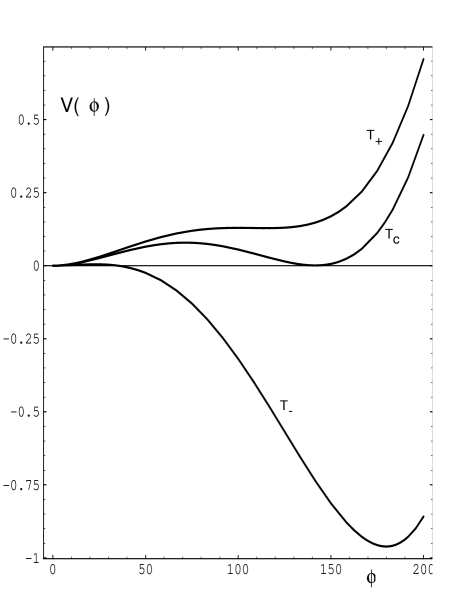
Figure 2: Effective potential evolution at first order phase transition.

The above remarks suggest that the equilibrium statistical mechanics may be applied for the evaluation of the “static” properties of the phase transitions, such as the critical temperature $T_{c}$, latent heat, jump of the order parameter (expectation value of the scalar field), interface tension (surface energy density of the plane domain wall separating different phases). Another important characteristics is the metastability range: at the upper $T_{+}$ (lower $T_{-}$ ) spinodial decomposition temperatures broken (symmetric) phase ceased to exist as a metastable state (fig. 2). The static correlation lengths for various operators may help to understand the structure of the domain walls.

The first order phase transition in the early Universe is not an instant process, and its total duration is of the order of the Universe age. The bubbles of the new phase start to nucleate at temperatures somewhat lower than $T_{c}$; the bubbles expand and finally fill out the Universe with the new phase. This happens at temperatures above $T_{-}$. The fraction of the volume of the Universe occupied by a new phase, ${\cal P}(t)$, can be estimated in the following way [136]. Suppose that the bubble nucleation rate per unit time per unit volume is ${\cal R}(T)$, and the velocity of the bubble walls is constant and equal to $v$. Then,

$${\cal P}(t)=1-\exp(-\Delta(t)),$$ (5.2)

where $V(t,t_{0})=\frac{4\pi}{3}v^{3}(t-t_{0})^{3}$ is the volume that the bubble nucleated at time $t_{0}$ occupies at time $t$:

$$\Delta(t)=\int_{t_{c}}^{t}dt_{0}~{}V(t,t_{0}){\cal R}(T(t_{0}))$$ (5.3)

and $t_{c}$ is the time corresponding to the critical temperature, $T(t_{c})=T_{c}$. This equation does not take into account the red shift of the bubble velocity, which is in fact unimportant at the electroweak scale. Introducing the variable

$$x=\frac{T_{c}-T}{T_{c}}$$

and assuming that it is small (this is satisfied in the electroweak case), one obtains a simplified expression

$$\Delta=\frac{64\pi v^{3}}{3}\left(\frac{M_{0}}{T_{c}}\right)^{4}\int_{0}^{x}\frac{{\cal R}(T)}{T_{c}^{4}}x^{3}~{}dx.$$ (5.4)

The phase transition is completed when

$$\Delta\simeq 1.$$ (5.5)

Since the electroweak scale is much smaller than the Plank scale, the probability of the bubble nucleation ${\cal R}$ at the percolation time is very small:

$$x^{3}\frac{{\cal R}(T)}{T_{c}^{4}}\sim\left(\frac{T_{c}}{M_{0}}\right)^{4}\sim\exp(-150).$$

The typical bubble size is of the order of $R\sim 2v\frac{M_{o}}{T_{c}^{2}}x$, where $x$ is to be found from eq. (5.5).

Computation of the bubble nucleation rate in the general case is a very complicated problem, which has not been solved. The reliable estimates exist only in the so-called thin wall approximation, and the leading contribution can be read off from the Landau–Lifshitz book on statistical mechanics. Suppose that the temperature of the system is $T<T_{c}$, and $x\ll 1$. Then the free energy of the critical bubble can be found from the minimization condition

$$\frac{\partial F}{\partial R}=0,~{}~{}~{}F(R)=4\pi R^{2}\sigma-\frac{4\pi R^{3}}{3}\Delta p,$$ (5.6)

where $\Delta p=Lx$ is the pressure difference, $L$ is the latent heat of the transition, and $\sigma$ is the surface tension. From the latter relation one immediately obtains

$${\cal R}=\kappa T_{c}^{4}\exp(-S(x)),$$ (5.7)

where the bounce action is given by

$$S(x)=\frac{16\pi\sigma^{3}}{3T_{c}L^{2}}\frac{1}{x^{2}}(1+O(x))$$ (5.8)

and corrections $O(x)$ are model dependent. Indeed, the domain wall thickness is of the order of the typical correlation length $\xi$ in the system, which means that the radius of the bubble is defined up to corrections of order $\xi$. This produces an uncertainty in the action $\delta S/S\sim\frac{L\xi x}{\sigma}$ and gives an obvious requirement of the validity of the thin wall approximation $R\gg\xi$. The calculations of the bounce action in various models can be found in ref. [131, 137].

If $R\sim\xi$, then the thin wall approximation breaks down, the nucleation rate cannot be expressed only through macroscopic parameters of the phase transition (latent heat and surface tension) at the critical point. In this case the phase transition is delayed and the Universe is supercooled in the symmetric phase. The calculation of the bubble nucleation rate in this case cannot be done for a generic gauge theory because of an infrared problem in the thermodynamics of the gauge fields (see below), but it is feasible for weakly coupled pure scalar theory. A detailed study of the bubble nucleation in the scalar mean field theory defined by potential (5.13) is contained in ref. [138]. Naturally, the bubble nucleation rate receives dependence on the scalar correlation length $\xi$ at the phase transition, in addition to the surface tension and the latent heat. We refer here to [131, 137, 139] for more details. The more complicated problem is to determine the prefactor in the expression for the bubble nucleation rate. Its computation in one-loop approximation in scalar models and electroweak theory has been done in refs. [140, 141, 142, 143].

5.2 Simple estimates

To describe the high temperature phase transitions in any given theory it is very important to have a relevant calculational formalism. The traditional tool is the effective potential for the scalar field $\phi$. It is defined as the value of the free energy of the system (pressure with the minus sign) in a uniform background field $\phi$. The minima of this potential correspond to the (meta)stable states of the system. The system undergoes a first order phase transition if there are two degenerate minima of this potential, separated by the energy barrier. In general, the effective potential is a gauge dependent quantity; perturbative calculations often produce complex terms. However, the values of the potential at its minima are gauge invariant; this allows for the gauge-invariant definition of the critical temperature and latent heat.

The following simple strategy (the drawbacks of which we discuss later) gives a reasonable qualitative description of the phase transitions and often allows fairly accurate estimates [144]:

Step No. 1. Take your model and calculate the one-loop high temperature effective potential $V(\phi,T)$.

Step No. 2. Define from it the critical temperature, jump of the order parameter, latent heat and surface tension with the use of the following equations.
–$T_{c}$ and order parameter $\phi_{c}$:

$$\frac{\partial V(\phi_{c},T_{c})}{\partial\phi_{c}}=0,~{}V(\phi_{c},T_{c})=V(0,T_{c}).$$ (5.9)

–Latent heat and surface tension:

$$L=T_{c}\frac{\partial}{\partial T_{c}}(V(\phi_{c},T_{c})-V(0,T_{c})),$$ (5.10)

$$\sigma=\int_{0}^{\phi_{c}}\sqrt{2V(\phi,T_{c})}~{}d\phi.$$ (5.11)

Step No. 3. Calculate the bubble nucleation rate in the thin wall approximation and compare it with the rate of the Universe expansion. Determine the bubble nucleation temperature and check the validity of the thin wall approximation. If it does not work, evaluate the bubble nucleation rate for a thick wall. To this end find O(3) symmetric configurations extremizing the 3d action

$$S=\frac{1}{T}\int~{}d^{3}x~{}\left[{\frac{1}{2}}(\partial_{i}\phi)^{2}+V(\phi,T)\right]$$ (5.12)

with the boundary condition $\phi\rightarrow 0$ at $x\rightarrow\infty$. The bubble nucleation rate is then ${\cal R}\sim\exp(-S)$.

An example is provided by the Minimal Standard Model. Here the one-loop effective potential in the high temperature approximation is (for simplicity, we take the case when the Higgs boson is sufficiently light, and neglect the effects of the $U(1)_{Y}$ interactions):

$$V(\phi,T)={\frac{1}{2}}\gamma(T^{2}-T^{2}_{-})\phi^{2}-{\frac{1}{3}}\alpha T\phi^{3}+{\frac{1}{4}}\lambda\phi^{4}.$$ (5.13)

For the standard model with the top quark mass $m_{\mbox{\scriptsize top}}$

$$\alpha=9g^{3}/(32\pi),\gamma={\frac{3}{16}}g^{2}+{\frac{1}{2}}\lambda+{m_{\mbox{\scriptsize top}}^{2}\over 2v^{2}},$$ (5.14)

and the lower metastability temperature $T_{-}$ is related to the Higgs mass $m_{H}^{2}=2\lambda v^{2}$ through

$$T_{-}={m_{H}\over\sqrt{2\gamma}}.$$ (5.15)

Due to the presence of the cubic term, the potential predicts the first order transition with the critical temperature

$$T_{c}={T_{-}\over\sqrt{1-{\frac{2}{9}}{\alpha^{2}\over\lambda\gamma}}}>T_{-}$$ (5.16)

and the jump of the order parameter

$${\phi(T_{c})\over T_{c}}={\frac{2}{3}}{\alpha\over\lambda}.$$ (5.17)

Phase transition gets weaker when the scalar self-coupling increases. This is seen from the behaviour of the order parameter, latent heat, and the surface tension, all of which decrease with the increase of $\lambda$. At large $\lambda$ the bubble nucleation rate can be determined in the thin wall approximation, while at small $\lambda$ ($\lambda\sim g^{3}$) it breaks down, and the phase transition occurs with considerable supercooling. Qualitatively, the one-loop description gives correct results, but concrete numbers may be quite different from those obtained by a more refined treatment. The effect of the Debye screening on the effective potential was discussed in refs. [145, 137, 146, 147], and the two-loop computation has been done in refs. [148, 149, 150, 151, 152, 153, 154, 155]. Various aspects of the phase transition were discussed in refs. [156, 157, 158, 159].

5.3 The infrared problem and factorization

It was realised by Linde and Gross, Pisarski and Yaffe a long time ago [160, 161] that the perturbation theory for non-Abelian gauge theories with small coupling constants inevitably breaks down at high temperatures, at least in the symmetric phase. The physical reason is that at high temperatures, instead of the usual 4-dimensional expansion parameter $g^{2}$ the relevant parameter is $\rho\sim g^{2}n_{B}(E)$, where $n_{B}(E)=[\exp(-E/T)-1]^{-1}$ is the Bose distribution function, $E$ is the typical energy of a given process in the plasma. At $E<T$ the expansion parameter is greater than that at zero temperatures, namely, $\rho\sim\frac{g^{2}T}{E}$, accounting for typical Bose amplification of the amplitudes. In the symmetric phase, gauge bosons are massless in perturbation theory, there is no infrared cutoff, and the expansion parameter can be arbitrarily large. In the broken phase the infrared cutoff is provided by the vector boson mass, and perturbation theory converges provided $\frac{g^{2}T}{m_{W}}\ll 1$. Below we will give a more formal description of the infrared catastrophe.

The fact that the perturbation theory breaks down at $T\neq 0$ poses non-trivial difficulties for the description of the phase transition. Indeed, the phase transition occurs when the free energy of the broken phase is equal to that of the symmetric phase; but the latter cannot be calculated perturbatively. The latent heat of the transition receives contributions from both the symmetric and broken phases, and the same is true for the surface tension. In the Universe the phase transitions occur when it is cooling, so that the initial phase is the one in which perturbation theory breaks down. For strongly first order phase transitions, the leading contribution to the above parameters comes from the broken phase, where perturbation theory is applicable; in that case the perturbative description may be reliable. However, the infrared problem is fatal for an attempt of the perturbative quantitative study of the weakly first order phase transitions. Unfortunately, direct Monte Carlo lattice simulations of high temperature gauge theories are not possible at present for realistic theories, containing chiral fermions, due to well known difficulties in discretisation of the chiral fermion determinant. The purely bosonic sector of the models can be put on 4d lattice, and extensive 4d numerical simulations have been carried out in refs. [162, 163, 164, 165, 166], for a summary of results see a nice review by Jansen [167].

Recently, an approach was suggested, which allows for a solution of the equilibrium problem of phase transitions in weakly coupled (at zero temperatures) gauge theories [152, 168, 107, 169]. It combines both perturbative analysis and numerical Monte Carlo methods. The main idea of the method is the factorization of the different scales appearing in the description of the high temperature plasma. At the first stage, a much simpler effective theory, incorporating all essential non-perturbative dynamics of the phase transition, is constructed by perturbative methods. The idea of this construction, known as dimensional reduction, goes back to the papers by Ginsparg [170], and by Appelquist and Pisarski [171]. It was developed in refs. [152, 168, 107, 169] in application to the phase transitions and applied later to hot QCD in ref. [172, 173, 174, 175, 176]. Different aspects of dimensional reduction were studied in refs. [177, 178, 179, 180, 181, 182]. At the second stage the effective 3-dimensional theory is analysed by non-perturbative methods (MC lattice simulations) . In the discussion below we follow ref. [107].

The idea of dimensional reduction comes from an observation that equilibrium finite temperature field theory is equivalent to Euclidean zero temperature field theory defined on a finite “time” interval $\beta=1/T$ supplied with periodic boundary conditions for bosons and antiperiodic ones for fermions.

Periodic and antiperiodic boundary conditions enable one to decompose Bose ($\phi$) and Fermi ($\psi$) fields in Fourier series with respect to the finite time interval,

$$\phi(x,\tau)=\sum_{n=-\infty}^{\infty}\phi_{n}(x)\exp(i\omega^{b}_{n}\tau),$$ (5.18)

$$\psi(x,\tau)=\sum_{n=-\infty}^{\infty}\psi_{n}(x)\exp(i\omega^{f}_{n}\tau),$$ (5.19)

where $\omega^{b}_{n}=2n\pi T,~{}\omega^{f}_{n}=(2n+1)\pi T$. Therefore, 4d finite temperature field theory is equivalent to the 3d theory with an infinite number of fields, and 3d boson and fermion masses are just frequencies $\omega^{b}$ and $\omega^{f}$. One can easily recognize here a perfect analogy to Kaluza–Klein theories with compact higher-dimensional space coordinates. The equilibrium dynamics of the theory is completely characterized by the set of Matsubara (imaginary time, or Euclidean) Green’s functions, $G_{n}(\omega_{i},\vec{k_{i}})$, where $\omega_{i}$ are discrete frequencies, $n$ is the number of legs. The static bosonic Green’s functions (fermionic Green’s functions are never static, since the fermion frequences are odd) play an important role for the phase transition. For example, the expectation value of the scalar field is just $G_{1}(0,0)$; the static correlation lengths can be extracted from two-point Green’s functions, etc.

Assume now that the theory is weakly coupled, and that the expectation value of the Higgs field in the broken phase is small enough, so that the vector boson masses are much smaller than the temperature. Then the description of the phase transition (i.e. static bosonic Green’s functions) can be derived within a simpler 3d theory, which contains only bosonic fields corresponding to the $n=0$ sector of Fourier decomposition. In loose terms,“superheavy” (we keep the word “heavy” for other fields defined below) fields are integrated out. This theory is valid up to momenta $k\ll T$. To specify the dynamics of the effective theory one writes down the most general 3d super-renormalizable Lagrangian, containing zero modes only, and determines its parameters by the matching condition. This condition requires that the 2-, 3- and 4-point one-particle irreducible Green’s functions, evaluated in the effective theory and in the full 4d theory are the same up to some power of the coupling constant. The effective theory approximately describes then all static Green’s fuctions of the high temperature 4d theory. As discussed in ref. [107], the maximum accuracy that can be reached with a super-renormalizable 3d theory is

$$\frac{\Delta G}{G}\sim O(g^{4}).$$ (5.20)

To be more explicit, take as an example the Minimal Standard Model Lagrangian. Then the 3d effective theory is an $SU(2)\times U(1)$ bosonic theory, which contains the Higgs doublet, the scalar triplet (zero component of the $SU(2)$ gauge field), and the scalar singlet (zero component of the $U(1)$ field) with the action

$$S = \int\!d^{3}x\biggl{\{}\frac{1}{4}G^{a}_{ij}G^{a}_{ij}+\frac{1}{4}F_{ij}F_{ij}+(D_{i}\Phi)^{\dagger}(D_{i}\Phi)+m_{3}^{2}\Phi^{\dagger}\Phi+\lambda_{3}(\Phi^{\dagger}\Phi)^{2}+\lambda_{B}B_{0}^{4}$$ (5.21)

$$+\frac{1}{2}(D_{i}A_{0}^{a})^{2}+\frac{1}{2}m_{D}^{2}A_{0}^{a}A_{0}^{a}+\frac{1}{4}\lambda_{A}(A_{0}^{a}A_{0}^{a})^{2}+\frac{1}{2}(\partial_{i}B_{0})^{2}+\frac{1}{2}m_{D}^{\prime 2}B_{0}B_{0}$$

$$+h_{3}\Phi^{\dagger}\Phi A_{0}^{a}A_{0}^{a}+h_{3}^{\prime}\Phi^{\dagger}\Phi B_{0}B_{0}-\frac{1}{2}\lambda_{AB}B_{0}\Phi^{\dagger}A_{0}^{a}\tau^{a}\Phi+\tilde{\lambda}_{AB}B_{0}^{2}A_{0}^{a}A_{0}^{a}\,\,\biggr{\}},$$

where $G^{a}_{ij}=\partial_{i}A_{j}^{a}-\partial_{j}A_{i}^{a}+g_{3}\epsilon^{abc}A^{b}_{i}A^{c}_{j}$, $F_{ij}=\partial_{i}B_{j}-\partial_{j}B_{i}$, $D_{i}\Phi=(\partial_{i}-ig_{3}\tau^{a}A^{a}_{i}/2+ig_{3}^{\prime}B_{i}/2)\Phi$, $D_{i}A_{0}^{a}=\partial_{i}A_{0}^{a}+g_{3}\epsilon^{abc}A_{i}^{b}A_{0}^{c}$, and $\Phi=(\phi_{3}+i\phi_{4},\phi_{1}+i\phi_{2})^{T}/\sqrt{2}$. The $\tau^{a}$’s are the Pauli matrices. The factor $1/T$ multiplying the action has been scaled into the fields and the coupling constants, so that the fields have the dimension GeV^1/2 and the couplings $g_{3}^{2}$, $\lambda_{3}$, $\lambda_{A}$, $\lambda_{AB}$ have the dimension GeV.

The complete one-loop calculation of the 3d coupling constants and two-loop calculation of the 3d masses of the effective theory can be found in ref. [152, 107]; we present here only simple tree relations for the coupling constants

$$g_{3}^{2}=g^{2}T,~{}g_{3}^{\prime 2}=g^{\prime 2}T,~{}\lambda_{3}=\lambda T,~{}h_{3}={\frac{1}{4}}g^{2}T~{},$$ (5.22)

$$h_{3}^{\prime}={\frac{1}{4}}g^{\prime 2}T,~{}\lambda_{A}=\lambda_{B}=\tilde{\lambda}_{AB}=0,~{}\lambda_{AB}=gg^{\prime}T$$

and one-loop relations for the doublet scalar mass

$$m_{3}^{2}(\mu)=-{\frac{1}{2}}m_{H}^{2}+T\biggl{(}\frac{1}{2}\lambda_{3}+\frac{3}{16}g_{3}^{2}+\frac{1}{16}g_{3}^{\prime 2}+\frac{1}{4}g_{Y}^{2}\biggr{)}$$ (5.23)

and triplet and singlet masses

$$m_{D}^{\prime 2} = \biggl{(}\frac{1}{6}+\frac{5n_{F}}{9}\biggr{)}g^{\prime 2}T^{2},$$ (5.24)

$$m_{D}^{2} = \biggl{(}\frac{2}{3}+\frac{1}{6}+\frac{n_{F}}{3}\biggr{)}g^{2}T^{2}.$$ (5.25)

Here $m_{H}$ is the zero temperature Higgs mass, $g_{Y}$ is the Yukawa coupling constant corresponding to the $t$-quark, $n_{F}=3$ is the number of fermion generations.

Clearly, is is much easier to study this 3d model than the initial 4d theory, since it contains much less degrees of freedom. Another important fact is that the only remnant of fermions is their contribution to the 3d masses and coupling constants.

An inspection of relations (5.23) and (5.25) shows that further simplification of the effective theory is possible. Indeed, at the tree level at $m_{3}^{2}<0$ the symmetry is broken, and at $m_{3}^{2}>0$ it is restored. In other words, the phase transition takes place near $m_{3}^{2}=0$. At this point the hierarchy $m_{3}^{2}\ll m_{D}^{2}$ and $m_{3}^{2}\ll m_{D}^{\prime 2}$ holds, allowing for the construction of the effective theory containing the Higgs doublet and $SU(2)\times U(1)$ gauge fields only. The “heavy” scale $\sim gT$ is integrated out, and the super-renormalizable Lagrangian of the effective theory is merely

$$L=\frac{1}{4}G^{a}_{ij}G^{a}_{ij}+\frac{1}{4}F_{ij}F_{ij}+(D_{i}\Phi)^{\dagger}(D_{i}\Phi)+\bar{m}_{3}^{2}\Phi^{\dagger}\Phi+\bar{\lambda}_{3}(\Phi^{\dagger}\Phi)^{2}.$$ (5.26)

In the one-loop approximation

$$\bar{m}_{3}^{2}(\mu)=m_{3}^{2}-\frac{1}{4\pi}\biggl{(}3h_{3}m_{D}+h_{3}^{\prime}m_{D}^{\prime}\biggr{)}$$ (5.27)

and $\bar{\lambda}_{3}=\lambda_{3}$ at the tree level. Higher order corrections to these relations can be found in ref. [152, 107]. In fact, the possibility of integrating out the heavy scale has a general character and can be applied to any gauge theory. The effective description in terms of the super-renormalizable Lagrangian for the “light” modes only provides an accuracy

$$\frac{\Delta G}{G}\sim O(g^{3}).$$ (5.28)

for Green’s functions for “light” (static gauge bosons and scalars) fields. This theory is valid for $k\ll gT$, but $k$ may be as large as $g^{2}T$. The effective potential for the scalar field in 3d coincides with the hard loop resummed potential in 4d at high temperatures [149, 151, 152].

Since all the four parameters of the 3d theory are dimensionful, the theory is uniquely fixed by three dimensionless ratios:

$$\qquad x\equiv{\bar{\lambda}_{3}\over\bar{g}_{3}^{2}},\qquad y\equiv\frac{\bar{m}_{3}^{2}}{\bar{g}_{3}^{4}},\qquad z\equiv\left({\bar{g}^{\prime}_{3}\over\bar{g}_{3}}\right)^{2}$$ (5.29)

and the overall scale $g_{3}^{2}$, on which the physics does not depend. The temperature variation changes the parameter $y$, while $x$ and $z$ depend on $T$ only through logarithmic corrections. So, we arrive at the important conclusion that the dynamics of the electroweak phase transition depends on one dimensionless number only ($x$) since $z$ is related to the known weak mixing angle, $z\simeq 0.3$, and $y$ is fixed by the requirement that the temperature is equal to the critical one. The dependence of the parameter $x$ on the physical Higgs mass in MSM was found in ref. [107], see fig. 3.

In fact, the 3d theory defined by (5.26) plays the role of the universal theory describing the phase transition not only in the Minimal Standard Model, but in many of its extensions, including sypersymmetry, two Higgs doublets, etc. [107]. Let us take as an example the two Higgs doublet model. The integration over the superheavy modes gives a 3d $SU(2)\times U(1)$ theory with an extra Higgs doublet in addition to the theory considered above. Construct now the one-loop scalar mass matrix for the doublets and find the temperatures at which one of its eigenvalues is zero. Take the higher temperature; this is the temperature near which the phase transition takes place. Determine the mass of the other scalar at this temperature. Generally, it is of the order of $gT$, and therefore, is heavy. Integrate this heavy scalar out together with the heavy triplet and singlet – the result is the simple $SU(2)\times U(1)$ model. In the case when both scalars are light near the critical temperature, a more complicated model, containing two scalar doublets, should be studied. It is clear, however, that this case requires fine tuning. The consideration of the phase transitions in the two Higgs doublet model at the one-loop level can be found in refs. [183, 184, 185, 186, 187, 188, 189, 190].

The same strategy is applicable to the Minimal Supersymmetric Standard Model (MSSM). If there is no breaking of colour and charge at high temperature (breaking is possible, in principle, since the theory contains squarks), then all degrees of freedom, excluding those belonging to the two Higgs doublet model, can be integrated out. We then return back to the case considered previously. The conclusion in this case is similar to the previous one, namely that the phase transition in the MSSM can be described by a 3d $SU(2)\times U(1)$ gauge–Higgs model, at least in a considerable part of the parameter space. A one-loop analysis of this theory was carried out in refs. [191, 192, 193, 194].

Of course, effective super-renormalizable 3d theories do not provide an exact description of the phase transitions. Parametrically, $\frac{\Delta G}{G}\sim O(g^{4})$ or $\sim O(g^{3})$ depending on the level of dimensional reduction. The numerical estimate of uncertainty is model dependent. For the standard electroweak theory, corresponding estimates were given in ref. [107], with the result that the effective description provides an accuracy $\sim 1\%$ for Higgs masses from $30$ GeV up to few hundred GeV. For smaller Higgs masses the phase transition is too strong and the vector boson masses are of the order of temperature, i.e. the assumption of the scale hierarchy does not hold; if the Higgs mass is close to the unitarity bound, the perturbation theory, used in the construction of the effective Lagrangian, breaks down.

To summarize this discussion, in order to study phase transitions in weakly coupled gauge theories, one may construct simpler 3d theories, parameters of which can be perturbatively calculated. This calculation is free from any infrared divergences, and its ultraviolet divergences are removed by the usual counterterms of the zero-temperature perturbation theory. A unique 3d theory plays a role of universal theory for the description of the phase transition in many 4d models. In particular, the strength of the electroweak phase transition depends on the unique number, $x=\bar{\lambda}_{3}/\bar{g}_{3}^{2}$.

5.4 Phase structure of 3d theory

The construction of the effective 3d theory is free from infrared divergences. However, the perturbative calculations in 3d are infrared divergent in the symmetric phase. This is easy to see by simple power counting. For example, the $N$-th loop contribution to the vacuum energy in 3d (with dimension GeV³) must contain the factor $(g_{3}^{2})^{N-1}$. Therefore, starting from $N=5$ some dimensionful parameter (say, the typical momentum scale $k$) should appear in the denominator of each term of the expansion, i.e. the expansion parameter is $g_{3}^{2}/k$. In the symmetric phase the infrared cutoff is absent, and perturbation theory breaks down. The first (logarithmically) divergent contribution in the vacuum energy appears in four loops and is of the order of $(g_{3}^{2})^{3}$, giving a contribution of the order of $g^{6}T^{4}$ to the free energy.

This means that the 3d theory should be treated in a non-perturbative way. At present, non-perturbative studies of the complete 3d $SU(2)\times U(1)$ model are absent, and most results were derived for an $SU(2)$ gauge–Higgs system. Let us consider first the general structure of the phase diagram of this theory. In the $SU(2)$ gauge–Higgs model there are no known local gauge invariant order parameters, which would acquire a non-zero value only in one of the two phases of the model. In other words, there is no symmetry breaking or restoration in this model, and the gauge symmetry is always intact (see, for instance refs. [195, 196]). An ordinary jargon, saying that the vector bosons are massless in the symmetric phase and massive in the broken one is incorrect, since vector degrees of freedom are massive at any choice of parameters. A good statistical analogue of this system is an ordinary liquid, which may undergo the first order liquid–vapour phase transition without restoration or breaking of any symmetry. The phase diagram of the latter system usually has a critical point, where the line of the first order phase transition ends. At this point the phase transition is of the second order, and there is a massless scalar excitation in the physical spectrum.

The absence of the true order parameter in the gauge–Higgs system suggests two possible phase diagrams in the $(x,y)$ plane, shown schematically in fig. 4. In the first case the line of the first order phase transitions has an end point at finite $x$, while in the second case the end point is at $x=\infty$. By dotted lines we show the upper and lower spinodial decomposition temperatures. In the first case there exists a critical scalar self-coupling above which there is no phase transition at all, while in the second case a first order phase transition occurs for all physical parameters. It is important for cosmological applications to clarify the type of the phase diagram. For example, if there exists an end point of the line of the first order phase transition, and the physical value of $x$ is to the right of this end point, then there is a smooth cross-over transition without any strong deviations from thermal equilibrium. In the latter case there are no observational consequences from the electroweak epoch.

The following approaches were applied to $SU(2)$ gauge–Higgs system: $\epsilon$ expansion [197], exact renormalization group approach [198, 199, 200, 201], Schwinger–Dyson equation [202], perturbation theory [152], and lattice Monte Carlo simulations [169, 203, 204]. The first two approaches favour the second type of the phase diagram, while the third one argues in favour of the end point of the critical line. In general, perturbation theory describes well different characteristics of the phase transition at small scalar self-coupling constants, while $\epsilon$-expansion is more suitable in the regime when $\lambda_{3}/g_{3}^{2}\gg 1$ [205, 206, 207]. The lattice MC simulations cannot resolve the order of the phase transition at large scalar self-coupling constant.

We shall review here the results from the lattice 3d MC simulations only [208, 209, 168, 169, 203, 210]. The comprehensive presentation of all existing approaches would make the discussion too lengthy; our emphasis on MC simulations is mostly because this is the only approach which is based on the first principles and does not require any extra assumptions. For example, $\epsilon$ expansion relies on the hope that $\epsilon=1$ may appear to be a small expansion parameter. Exact renormalization group approach requires some truncation of the equations, and Schwinger–Dyson equations are constructed with the use of the perturbation theory which may appear to be not applicable. The lattice MC simulations produce a set of “true” characteristics of the phase transition (provided the quality of the data is such that extrapolation to the continuum limit is possible), which then can be used in cosmological applications. Of course, MC simulations do not provide an analytical understanding of the dynamics of the transition, but they may be considered as an “experimental” basis for construction or testing of different theories of the phase transitions. The lattice MC simulations fail to describe very weakly first order phase transitions. However, only sufficiently strong first order electroweak phase transition is of interest for cosmology, i.e. the lattice simulations can cover the entire interesting range of parameters.

5.5 The lattice formulation

The 3d gauge theory defined by the action

$$S=\int\!d^{3}x\biggl{\{}\frac{1}{4}G^{a}_{ij}G^{a}_{ij}+(D_{i}\Phi)^{\dagger}(D_{i}\Phi)+m_{3}^{2}\Phi^{\dagger}\Phi+\lambda_{3}(\Phi^{\dagger}\Phi)^{2}\biggr{\}}$$ (5.30)

has a number of remarkable properties. It contains only dimensionful coupling constants, and, therefore, it is super-renormalizable. The only ultraviolet infinities are those in the scalar mass renormalization, while the $\beta$ functions for $g_{3}^{2}$ and $\lambda_{3}$ are equal to zero. The exact $\beta$ function for the mass parameter is known [152],

$$\mu\frac{\partial m_{3}^{2}(\mu)}{\partial\mu}=-\frac{1}{16\pi^{2}}f_{2m},$$ (5.31)

where

$$f_{2m}={51\over 16}g_{3}^{4}+9\lambda_{3}g_{3}^{2}-12\lambda_{3}^{2}.$$ (5.32)

The lattice version of the continuum theory (5.30) is defined by the following action:

$$S = \beta_{G}\sum_{x}\sum_{i<j}\left(1-{\frac{1}{2}}{\rm Tr\,}P_{ij}\right)+$$

$$- \beta_{H}\sum_{x}\sum_{i}{\frac{1}{2}}{\rm Tr\,}\Phi^{\dagger}(\mbox{\bf x})U_{i}(\mbox{\bf x})\Phi(\mbox{\bf x}+i)+$$

$$+ \sum_{x}{\frac{1}{2}}{\rm Tr\,}\Phi^{\dagger}(\mbox{\bf x})\Phi(\mbox{\bf x})+\beta_{R}\sum_{x}\bigl{[}{\frac{1}{2}}{\rm Tr\,}\Phi^{\dagger}(\mbox{\bf x})\Phi(\mbox{\bf x})-1\bigr{]}^{2}.$$

Here $U_{i}(x)$ and $P_{ij}$ are the link and plaquette variables, and $\Phi$ is the scalar field. The action depends on the three dimensionless parameters $\beta_{G},\beta_{H},\beta_{R}$ (recall that the continuum dynamics is completely described by two numbers, $x$ and $y$). The fact that the theory under consideration is super-renormalizable enables one to find an exact (in the continuum limit) matching between the lattice variables and the physical parameters. The corresponding calculation has been carried out in refs. [168, 211]; it provides the relation between the lattice renormalization scheme and the $\overline{\mbox{\rm MS}}$ scheme in continuum. The continuum limit is $\beta_{G}\rightarrow\infty,~{}\beta_{H}\rightarrow{\frac{1}{3}},~{}\beta_{R}\rightarrow 0$ in such a way that the physical parameters $x$ and $y$, defined as

$$x = {1\over 4}\lambda_{3}a\beta_{G}={\beta_{R}\beta_{G}\over\beta_{H}^{2}},$$ (5.34)

$$y = {\beta_{G}^{2}\over 8}\biggl{(}{1\over\beta_{H}}-3-{2x\beta_{H}\over\beta_{G}}\biggr{)}+{3\Sigma\beta_{G}\over 32\pi}(1+4x)+$$ (5.35)

$$+{1\over 16\pi^{2}}\biggl{[}\biggl{(}{51\over 16}+9x-12x^{2}\biggr{)}\biggl{(}\ln{3\beta_{G}\over 2}+\zeta\biggr{)}+\eta+\bar{\eta}x\biggr{]}$$

stay constant. Equation (5.35) depends on several constants arising from lattice perturbation theory; $\Sigma=3.17591$, $\zeta=0.09$, $\eta=5.0$ and $\bar{\eta}=5.2$ were computed in refs. [168, 211].

If we denote by $a$ the lattice spacing which has dimension of length, then the overall continuum scale $g_{3}^{2}$ is related to it as

$$g_{3}^{2}a={4\over\beta_{G}},$$ (5.36)

i.e. the continuum limit corresponds to $a\rightarrow 0$. The relation of the lattice variables to the continuum fields in this limit is

$$\Phi=VR_{L},\quad R_{L}^{2}={2a\over\beta_{H}}\phi^{\dagger}\phi={\frac{1}{2}}{\rm Tr\,}\Phi^{\dagger}\Phi,\quad U_{i}=\exp\left({\frac{1}{2}}iag_{3}\tau_{a}A_{i}^{a}\right),$$ (5.37)

where $V$ is a unitary SU(2) matrix, $R_{L}$ is the radial mode of the Higgs field, $\tau_{a}$ are the Pauli matrices.

Equations (5.34) and (5.35) serve as the basis for relating the results of the lattice simulations to the physical reality. We are not going to discuss here technical details of the lattice simulations [169]. Instead, we review the general strategy for the lattice study of the phase transition. The reader not familiar with MC computations may consider the computer as a device for calculating the Euclidean functional integral

$$\langle O(A,\phi)\rangle=\frac{\int~{}DAD\phi~{}O(A,\phi)\exp(-S)}{\int DAD\phi\exp(-S)},$$ (5.38)

where $O(A,\phi)$ is some gauge-invariant functional of the gauge and scalar fields, and $S$ is the lattice action. The integral should be computed for different volumes of the system and different lattice spacings, and extrapolation of the results to the infinite volume and zero $a$ must be taken at the end. By choosing the specific $\delta$-function form of this functional,

$$O=\delta(c-G(A,\phi))$$ (5.39)

one can construct probability distributions for various order parameters $G(A,\phi)$, essential for the study of the phase transition.

The critical temperature. Let us fix $\beta_{G}$ (i.e. the ultraviolet cutoff) and vary parameters $\beta_{H}$ and $\beta_{R}$ in such a way that the physical variable $x$ stays constant. In 4d language this corresponds to varying the temperature. The existence of the first order phase transition means that at some critical value of $\beta_{H}$ there are two degenerate ground states with different properties. In particular, expectation values of the gauge invariant observables are different in distinct states. For example, the average value of $R^{2}$ is expected to be smaller in the symmetric phase than in the Higgs phase. This means that the probability distribution at the critical point has non-trivial form and contains two peaks rather than one. The typical picture of the distribution evolution is shown in fig. 5. At large $\beta_{H}$ (low temperatures) there is a unique value of the order parameter $R^{2}$, corresponding to the Higgs phase, while at some $\beta_{H}$ a double peak stucture develops, signalling about the first order phase transition. The critical value of $\beta_{H}$ can be found from the requirement that the areas under the two peaks are equal to each other. Of course, it must be checked that the double peak structure is not a lattice artefact and passes different tests singling out the first order behaviour [169]. After the critical value of $\beta_{H}$ is found, it may be converted to the critical temperature of the underlying 4d theory.

The latent heat. The latent heat $L$ — the energy released in the transition — can be calculated from

$${\frac{L}{T}}={\frac{d\Delta p}{dT}}={\frac{T}{V}}{\frac{d}{dT}}\Delta\log Z={\frac{T}{V}}{\frac{d}{dT}}\Delta P\,,$$ (5.40)

where the derivatives are evaluated at the critical temperature, $\Delta p$ is the difference of the pressures in the symmetric and broken phases, and $\Delta P$ is the difference in the probabilities of the phases in volume $V$. In eq. (5.40), $T$ is the physical (4d) temperature. The quantity $\Delta P$ is directly proportional to the difference of the areas under the two peaks in the order parameter distributions near $T_{c}$; it may be computed by performing simulations at $\beta_{H}$ close to the critical one.

The jump of the order parameter. The order parameter usually discussed in the study of the effective potential is the vacuum expectation value $v$ of the Higgs field. This quantity, however, is not gauge invariant. The gauge-invariant substitute of it is the scalar condensate $\langle\phi^{\dagger}\phi\rangle$. This is a composite operator, whose expectation value contains linear divergence at the one-loop level and logarithmic divergence at the two-loop level. These divergences can be removed, e.g. by the $\overline{\mbox{\rm MS}}$ prescription; the resulting condensate is then dependent on the scale parameter $\mu$. Because of the fact that the 3d theory is super-renormalizable, an exact relation between the lattice quantity $\langle R^{2}\rangle$ and $\langle\phi^{\dagger}\phi\rangle$ can be found [168],

$${\langle\phi^{\dagger}\phi(\mu)\rangle\over g_{3}^{2}}={\frac{1}{8}}\beta_{G}\beta_{H}\biggl{(}\langle R^{2}\rangle-{\Sigma\over\pi\beta_{H}}\biggr{)}-{3\over(4\pi)^{2}}\biggl{(}\log{3\beta_{G}g_{3}^{2}\over 2\mu}+\zeta+{\frac{1}{4}}\Sigma^{2}-\delta\biggr{)}+O\left(\frac{1}{\beta_{G}}\right).$$ (5.41)

Numerically $\zeta+{\frac{1}{4}}\Sigma^{2}-\delta=0.67$. Thus, the extrapolation of lattice measurements of the quantity $\langle R^{2}\rangle$ to the limit $\beta_{G}\rightarrow\infty$ allows one to determine an “exact” value of the scalar condensate. The comparison of the lattice results with known two-loop perturbative expansion allows the extraction of the magnitude of the higher order perturbative terms. In this way a three-loop correction to the effective potential has been numerically determined in ref. [169]. For estimates, the relation ${\frac{1}{2}}\frac{v^{2}}{T^{2}}=\langle\phi^{\dagger}\phi(T)\rangle/T$ can be used. The effective potential for the gauge-invariant condensate was constructed in ref. [212].

The jump of the quantity $\langle\phi^{\dagger}\phi\rangle$ at the phase transition (difference between condensates in the broken and symmetric phases at the critical temperature) is a finite and scale independent quantity, which can be directly measured on the lattice as the distance between the positions of the two peaks in the $R^{2}$ distribution,

$$\Delta(\langle\phi^{\dagger}\phi\rangle)={\frac{1}{8}}g_{3}^{2}\beta_{G}\beta_{H}\Delta(\langle R^{2}\rangle).$$ (5.42)

It can be shown that $\Delta(\langle\phi^{\dagger}\phi\rangle)$ is directly related to the latent heat of the transition [168, 169, 213].

The interface tension. The interface tension is one of the most important quantities which characterize the strength of the phase transition. It can be measured by constructing probability distributions of some local order parameter. At the critical temperature, a system in finite volume predominantly resides in either the Higgs or the symmetric phase, but it can also exist in a mixed state consisting of domains of the two states. The probability of the mixed state is suppressed by the extra free energy associated with the interfaces between the phases. This causes the typical two-peak structure of the probability distribution of the order parameter at the critical temperature (see fig. 6): the midpoint between the peaks corresponds to a state which consists of equal volumes of the symmetric and broken phases. Because of the associated extra free energy, the area of the interfaces tends to minimize. Assuming lattice with periodic boundary conditions and geometry $L_{x}^{2}\times L_{z}$, where $L_{x}\leq L_{z}$, the minimum area is $2\times A=2(L_{x}a)^{2}$ — the factor 2 appearing because there are two separate interfaces. The interface tension $\sigma$ can be extracted from the limit

$${\frac{\sigma}{T}}=\lim_{V\rightarrow\infty}{\frac{1}{2A}}\log{\frac{P_{\rm max}}{P_{\rm min}}}\,$$ (5.43)

where $P_{\rm max}$ is the maximum of the probability distribution in the peak and $P_{\rm min}$ is the minimum of distribution between the peaks in fig. 6. At sufficiently large size of the system in the $z$ direction, the probability distribution has a characteristic plateau, corresponding to the translational zero mode of the domain wall. Other methods for determination of the surface tension are discussed in [165, 166], the estimate of the higher order perturbative corrections is contained in ref. [214].

5.6 Some lattice results

The 3d lattice simulations have been made for four values of the continuum parameter $x$, namely, $x=0.01830,~{}0.06444,~{}0.08970$ and $x=0.1188$ [169, 210]. These values correspond to different 4d physical parameters in different models. For definiteness, let us take the $SU(2)$ sector of the standard model with top quark mass $m_{t}=175$ GeV. Then the first value of $x$ cannot be realized with any value of the Higgs mass (see fig. 3), while the others correspond to $m_{H}\approx 51.2,~{}68.0$ GeV and $\approx 81$ GeV, respectively. The latter numbers come from the one-loop relations between the $\overline{\mbox{\rm MS}}$ and physical parameters of the standard model and the one-loop dimensional reduction [107]. Because of the large value of the top Yukawa coupling constant the one-loop corrections are quite substantial for small Higgs masses, for example $\delta m_{H}/m_{H}\sim 15\%$ for $m_{H}\approx 50$ GeV. A naive estimate of the two-loop corrections (taken as square of the one-loop contribution) indicates that the accuracy of the one-loop computation of the physical masses at fixed 3d parameter $x$ is $\sim 2\%$ for $x=0.06444$ and better for larger $x$.

For the “large” value of the Higgs mass ($81$ GeV) it was not possible to resolve the order of the phase transition on the lattices up to $48^{3}$, and the data are compatible with the smooth cross-over, second order phase transition or very weakly first order phase transition. For smaller Higgs masses the transition is of the first order.

The most complete study has been done for $x=0.06444$. This value may be quite realistic for extended versions of the electroweak theory, but is excluded experimentally in the MSM (it corresponds to $m_{H}\approx 51.2$ GeV). Below we present the specific numbers for MSM with $m_{t}=175$ GeV, derived with the use of one-loop relations. The critical temperature of the phase transition is $T_{c}=89.79$ GeV, and the vev-to-temperature ratio at $T_{c}$ is $v/T_{c}=0.64$. The domain wall separating the broken and symmetric phases has the surface tension $\sigma\simeq 0.002T_{c}^{3}$, and the latent heat is $L/T_{c}^{4}=0.12$. At $T>T_{+}=89.93$ GeV only the symmetric phase is stable, and at $T<T_{-}=89.36$ only the broken phase is stable, while at temperatures between $T_{-}$ and $T_{+}$ both phases can exist simultaneously. The scalar correlation lengths in the symmetric and Higgs phases are $\sim 6/T_{c}$ and $\sim 8/T_{c}$, respectively. The statistical errors of the lattice numbers are $0.015\%$ for the critical temperature, $1\%$ for the expectation value of the Higgs field and the latent heat, and $\sim 20\%$ for the interface tension. The two-loop corrections may introduce extra uncertainties in these numbers of the order of $2\%$.

The bubble nucleation temperature $T_{\rm bubble}$ lies somewhere between $T_{c}$ and $T_{-}$ and may be estimated with the use of the surface tension and latent heat found on the lattice. Inserting the lattice numbers to the relations (5.5), (5.8), (5.7) gives an estimate $\frac{\Delta T}{T_{c}}\simeq 0.0004$, i.e. the bubble nucleation temperature is very close to the critical one. The smallness of ${\Delta T}/{T_{c}}$ is due to fact that the ratio $\sigma^{3}/L^{2}T_{c}\sim 2\cdot 10^{-6}$ is so small [215]. Since $\Delta T/(T_{c}-T_{-})\simeq 0.1$ is also small, one is in the thin wall regime; indeed, the size of the bubbles when they nucleate is at least $R_{c}\simeq 110/T_{c}$, which is much larger than the scalar correlation length in either the broken or the symmetric phase at $T_{\rm bubble}$. Because $T_{\rm bubble}$ is very close to the critical temperature, the expectation value of the Higgs field at $T_{\rm bubble}$ is almost the same as at $T_{c}$. In other words, the transition is very weakly first order.

The lattice results can be compared with the perturbative calculations of the two-loop effective potential. The predictions of the critical temperature, latent heat, and the jump of the order parameter appear to be quite reasonable and are within a few per cent for these quantities. However, perturbation theory fails to describe the surface tension (and, therefore, the bubble nucleation rate) at least for $x=0.06444$: the perturbative value is about 3 times larger than the lattice one.

5.7 Dynamics of the phase transition

In the case of the “vacuum phase transitions” – false vacuum decay at zero temperatures – the energy stored in the metastable vacuum transforms into kinetic energy of the domain walls [126, 127]. As a result, the velocity of a domain wall increases and approaches the speed of light. Then in the collisions of domain walls, their kinetic energy is released and transforms into heat, and the system is reheated up to a certain temperature.

At non-zero temperatures nucleated bubbles expand in the medium, and the latent heat of the transition may be released by many different mechanisms. In the idealistic case of the very slow expansion of the Universe, the temperature stays constant during the phase transition, fig. 7 (see, e.g. ref. [138]). Every point on the plateau corresponds to a mixed state containing domains of broken and symmetric phase; the left point of the plateau corresponds to the pure symmetric phase, and the right point to the pure broken phase. The release of the latent heat of the transition is accommodated by the Universe expansion.

In fact, the Universe expands not so slowly at the electroweak scale and is supercooled in the symmetric phase. One can distinguish several different epochs in the phase transition. The first one is the bubble nucleation, the second one is the bubble growth, the third one is the bubble percolation – the period when different bubbles collide. At this stage the Universe may be reheated up to the critical temperature (fig. 7). If it happens, then the later evolution may be close to an ideal case described above.

We have already discussed the bubble nucleation rate and determination of the bubble nucleation temperature $T_{b}$. Let us now consider the bubble expansion from macroscopic point of view in more detail [216, 217, 138, 218, 156, 219, 215, 220, 221].

Initially, the bubble of a new phase is a microscopic object with a size of several correlation lengths. At the bubble nucleation temperature the energy density in the symmetric phase is larger than that in the broken phase,

$$\epsilon_{sym}=\frac{\pi^{2}}{30}N_{eff}T^{4},~{}~{}\epsilon_{Higgs}=\frac{\pi^{2}}{30}N_{eff}T^{4}-L.$$ (5.44)

Here $N_{eff}=N_{b}+{\frac{7}{8}}n_{f}$ is the effective number of the massless degrees of freedom and $L$ is the latent heat. For the Minimal Standard Model $N_{eff}=106{\frac{3}{4}}$. The general hydrodynamical consideration of the bubble evolution leads to two possible types of bubbles, known as deflagration and detonation bubbles [216, 217].

Consider an isolated macroscopic bubble. For a large enough bubble, its curvature may be neglected and the interface may be taken as a planar domain wall . Let us proceed in the rest frame of the domain wall and denote by $v_{1}$ the velocity of the medium falling on the domain wall (symmetric phase) and by $v_{2}$ the velocity of the medium inside the bubble. Then, if $v_{1}<c_{s}$, where $c_{s}\simeq\frac{1}{\sqrt{3}}$ is the velocity of sound in the medium, then the phase transition proceeds through deflagration. In this case the medium is accelerated when it passes through the domain wall, $v_{2}>v_{1}$. If, on the contrary, $v_{1}>c_{s}$, then $v_{1}>v_{2}$, and we have detonation bubbles. The realization of one of the two mechanisms of the bubble walls propagation depends on the relationship between the latent heat of the transition, surface energy density, and the rate of entropy generation on the phase boundary [217]. The latter is to be found from the microscopic analysis of the interaction of particles with the bubble walls [223, 137, 224, 225, 226, 227, 228].

If we now choose the reference frame to be the rest frame of the plasma before the bubble has nucleated, then the medium should be at rest in the centre of the bubble and far from it. Then, for the deflagration bubbles the medium in front of the bubble wall is accelerated by the motion of the wall, and there is a shock wave in the symmetric phase moving with the velocity $v_{shock}>v_{b}$, and $v_{b}=v_{2}$ is the bubble wall velocity. The velocity of the symmetric phase plasma between the shock front and the bubble wall is given by $v_{sym}=(v_{2}-v_{1})/(1-v_{1}v_{2})$. The temperature of the medium between the shock front and the bubble wall $T_{shock}$ and the temperature inside the bubble $T_{r}$ are different from the bubble nucleation temperature (temperature outside the shock front) $T_{b}$. They depend in general on the distance from the bubble centre. Usually the inequality $T_{b}<T_{r}<T_{shock}$ holds true [217], but $T_{r}<T_{b}$ at high rates of entropy generation at the domain walls [215]. The latent heat of the transition transforms into the kinetic energy of the plasma in the symmetric phase, and to heating of the plasma inside the shock wave front.

The detonation bubbles have a different structure. The velocity of the domain wall is larger than the speed of sound, the symmetric phase plasma is at rest right in front of the domain wall and has temperature $T_{b}$. The plasma just behind the wall (in the Higgs phase) is accelerated by it and has velocity $v_{br}=(v_{1}-v_{2})/(1-v_{1}v_{2})$. Finally, the plasma is stopped at some surface inside the bubble by a rarefaction wave. As in the previous case, the temperatures inside the front of the rarefaction wave $T_{r}$ and behind the bubble wall $T_{br}$ are different from $T_{b}$.

The recent analysis carried out in ref. [228, 227] suggests that for a sufficiently wide range of the parameter space of the standard model, $m_{H}<90$ GeV, an isolated bubble expands as a weak deflagration (“weak” means that the velocity of the bubble wall is subsonic). The velocity $v_{b}$ was found to be in the range $0.38<v_{b}<0.45$, while the velocity of the shock front is close to the speed of sound in the medium, $v_{shock}\simeq c_{s}\simeq 0.58$. When the shocks coming from different bubbles begin to collide, the single bubble approximation breaks down. At this time, roughly, a $(v_{b}/c_{s})^{3}\simeq 0.3$ part of the Universe volume is in the broken phase. The subsequent evolution of bubbles depends on the temperature in the symmetric phase, which will emerge as a result of shock waves interaction. This temperature can be estimated as follows [215, 229]. Suppose that all latent heat of the transition is immediately released in form of heat in the broken phase. Then the reheating temperature can be found from energy conservation condition,

$$\frac{\pi^{2}}{30}N_{eff}T_{b}^{4}=\frac{\pi^{2}}{30}N_{eff}T_{r}^{4}-L,$$ (5.45)

so that

$$\frac{T_{r}-T_{b}}{T_{c}}=\frac{15}{2\pi^{2}N_{eff}}\frac{L}{T^{4}}.$$ (5.46)

Now, if $\frac{T_{c}-T_{b}}{T_{c}}\gg\frac{T_{r}-T_{b}}{T_{c}}$, then the reheating process may be neglected. However, in the opposite case the heat release is important and the expansion of the bubbles of a new phase should slow down.

Simple estimates can be done in a thin wall approximation. The bubble nucleation temperature is given by

$$\frac{T_{c}-T_{b}}{T_{c}}=\sqrt{\frac{16\pi\sigma^{3}}{3L^{2}T_{c}S_{0}}},$$ (5.47)

where $S_{0}\simeq 160$ is the action for the critical bubble and $\sigma$ is the surface tension. For example, for the Minimal Standard Model with $m_{H}=51.2$ GeV and $m_{t}=175$ GeV we get $T_{c}=88.93$ GeV, $L/T^{4}=0.124$, $\sigma/T^{3}=0.0023$ [169], and

$$\frac{T_{r}-T_{b}}{T_{c}}=9\cdot 10^{-4}>\frac{T_{c}-T_{b}}{T_{c}}=3\cdot 10^{-4}.$$ (5.48)

So, for this choice of parameters the Universe should reheat to the critical temperature, the speed of the domain walls is greatly reduced, the broken phase bubbles expand slowly due to the Universe expansion. At the final stage of the phase transition the remnants of the symmetric phase shrink, again due to the Universe expansion. This picture is also true for higher values of the MSM Higgs masses, provided the phase transition is still of the first order.

An estimate of the bubble wall velocity at a late stage of the phase transition (under the assumption that the Universe is reheated up to the critical temperature) can be found from a simple thermodynamical consideration [230] (see also ref. [229]). Suppose that the average bubble size is $R_{b}$, and that the part of the volume of the space occupied by the broken phase is ${\cal P}$. Then the requirement that the Universe expands adiabatically is given by

$$\frac{{\dot{R_{b}}}}{R_{b}}{\cal P}L=sH,$$ (5.49)

where $s$ is the entropy density in the symmetric phase, $s=\frac{2\pi^{2}}{45}N_{eff}T^{4}$, and $H$ is the Hubble constant. The average bubble size can be found from the following consideration. The (non-normalized) distribution of the bubbles in sizes at moment $t$ is given by

$$P(R,t)dR\sim{\cal R}(t_{1}),$$ (5.50)

where ${\cal R}(t_{1})$ is the bubble nucleation probability at time $t_{1}$, and $t_{1}$ is related to $R$ and $t$ by the obvious condition that $t_{1}=t-\frac{R}{v_{b}}$. Then

$$\langle R\rangle(t)=\frac{\int~{}R~{}P(R,t)~{}dR}{\int~{}P(R,t)~{}dR}.$$ (5.51)

In the thin wall approximation

$${\cal R}(t)\sim\exp\left(-\frac{AT_{c}^{2}}{4(T_{c}-T)^{2}}\right)\sim\exp\left(-\frac{At_{c}^{2}}{(t-t_{c})^{2}}\right)$$ (5.52)

with $A=\frac{64\pi\sigma^{3}}{3L^{2}T_{c}}$, and $t_{c}$ is the time corresponding to the temperature $T_{c}$. The average bubble radius at time $t$ is

$$\langle R\rangle(t)\simeq{\frac{1}{2}}v\frac{(t-t_{c})^{3}}{At_{c}^{2}}$$ (5.53)

and at the percolation temperature it is about $\langle R\rangle(t)\simeq{\frac{1}{2}}v_{b}t_{c}\frac{\sqrt{A}}{\sqrt{S_{0}^{3}}}$. For example, for the numerical values of the parameters given above one finds $A\simeq 5.3\cdot 10^{-5},~{}HR_{b}\simeq 10^{-6}$ and

$${\dot{R}}=v_{b}\simeq\frac{s}{L}\frac{HR_{b}}{{\cal P}}\sim 10^{-3}$$ (5.54)

for ${\cal P}\sim 0.3$. This value gets larger if the scalar self-coupling is decreased. For example, for stronger phase transition the reheating up to the critical temperature may occur, and the velocity of the domain wall from the estimate of ref. [229] may be higher by a factor $\sim 10$.

Of course, the estimates given above are rather rough since they are based on the assumption of the instantaneous latent heat release. Nevertheless, they show that it is quite plausible that the slow stage of the phase transition takes place for the interesting range of the parameters of the underlying theory [229].

6 Survival of primordial baryon asymmetry

The anomalous electroweak processes are rapid at sufficiently high temperatures. Their rate $\Gamma_{sph}$ exceeds the rate of the Universe expansion $\frac{T^{2}}{M_{0}}$ in the standard Big Bang scenario in the following interval of temperatures:

$$100\mbox{GeV}\sim T^{*}<T<T^{**}\simeq\alpha_{W}^{4}M_{Pl}\simeq 10^{12}\mbox{GeV},$$ (6.1)

where the lower temperature $T^{*}$ is to be found from the condition of decoupling of the sphaleron processes in the broken phase of the EW theory [231, 232],

$$\frac{M_{sph}(T^{*})}{T^{*}}\simeq 45.$$ (6.2)

Clearly, the equilibrium character of $B$-violating reactions has an important impact on the survival of the primordial baryon asymmetry. Several different cases can be distinguished, depending on initial conditions and on the rate of $B$ and $L$ non-conservation due to processes other than those associated with sphalerons.

(i) Suppose that the Universe is asymmetric with respect to the anomaly free fermionic charges $\Delta_{i}=L_{i}-\frac{1}{n_{f}}B$ of the standard model at $T>T^{**}$, and assume that at $T<T^{**}$ there is no $B$ or $L$ violating interactions besides the electroweak anomalous processes. The origin of the primordial asymmetry is not essential here. Then anomalous reactions convert the initial asymmetry to the baryonic one at $T=T^{*}$. For the minimal standard model the relationship is given by [94, 75] (see also [96, 97]),

$$\Delta_{0}=\frac{8n_{f}+4}{22n_{f}+13}\Delta_{B-L}-K\frac{4}{13\pi^{2}}\sum_{i=1}^{n_{f}}\frac{m_{i}^{2}(T^{*})}{(T^{*})^{2}}\Delta_{i}.$$ (6.3)

where $m_{i}^{2}$ is the lepton mass of a given generation, $K\approx 1$. The first term in the right hand side of this equation tells that $(B-L)$ asymmetry is reprocessed into the baryon asymmetry, while $(B+L)$ tends to be washed out; the second term is the correction coming from slightly different behavior of quarks with different masses in the plasma. If the initial value of $(B-L)$ is non-zero (coming, say, from the GUT physics) then the baryon asymmetry, up to a possible contribution from the EW phase transition (see below), has a primordial character. If, on the contrary, the initial $B-L$ asymmetry is absent, we can rely only on the second term in (6.3). For three lepton generations one gets a suppression $\Delta_{0}\simeq 3\times 10^{-6}\Delta_{3}$. So, to have a non-negligible effect, the initial asymmetry $\Delta_{3}$ must be very large, or the standard theory should be extended by adding heavy leptons.

(ii) Suppose now that there are some reactions, which do not conserve all $\Delta_{i}$, and which are in thermal equilibrium for some period between $T^{*}$ and $T^{**}$. At this intermediate epoch $B$ and $L$ are non-conserved separately, and according to the third Sakharov condition all baryonic and leptonic asymmetries are washed out. Hence, the existence of these reactions is fatal for the primordial baryon asymmetry. If the baryon asymmetry is not produced at a later time, the requirement of the absence of these reactions may appear to be a powerful tool for constraining the properties of new particle interactions [233, 96, 234, 235]. However, some time ago it was realized that most of these constraints are drastically weakened due to the smallness of some Yukawa coupling constants in the standard model or its supersymmetric extensions [236, 237, 238, 239, 240, 241].

Let us discuss the main idea of these estimates on the example of lepton number violating interactions, leading to the Majorana neutrino masses $m_{ij}$ [240]. We take for simplicity the Minimal Standard Model and add to it lepton number violating interactions. The $SU(2)\times U(1)$ symmetric low energy Lagrangian with $\Delta L=2$ has the form

$$\frac{1}{v^{2}}m_{ij}(\bar{L_{i}}\phi)(\tilde{\phi}^{\dagger}L_{j}^{c}),$$ (6.4)

where $L_{i}$ and $L_{j}^{c}$ are lepton doublet and its charge conjugate, respectively, $\phi$ is the scalar doublet, $v$ is the vacuum expectation value of the Higgs field $v=246$ GeV. The rate of $L$ non-conserving reactions $L\phi\rightarrow L^{c}\phi^{*}$ at high temperatures has been found in ref. [240]

$$\Gamma\simeq\frac{9}{\pi^{5}}\frac{T^{3}}{v^{4}}\bar{m}_{\nu}^{2},$$ (6.5)

where $\bar{m}_{\nu}$ is an average Majorana neutrino mass,

$$\bar{m}_{\nu}^{2}={\frac{5}{3}}|m_{ee}|^{2}+|m_{e\mu}|^{2}+|m_{e\tau}|^{2}.$$ (6.6)

These reactions were initially required [96] to be out of thermal equilibrium at $T<T^{**}$; this leads to a very stringent constraint

$$\bar{m}_{\nu}<\frac{v^{2}}{\sqrt{M_{0}T^{**}}}\simeq 10^{-2}\mbox{eV}.$$ (6.7)

An implicit assumption in the derivation above is that the set of conserved numbers $\Delta_{i}$ is a complete one below $T=T^{**}$. In fact, this is not true due to the smallness of the right-handed electron Yukawa coupling constant. In the limit when this constant is zero, the right-handed electron number is conserved, and the asymmetry in it propagates to the asymmetry in baryon number. The rate of reactions not conserving the right-handed electron number (say, $e_{L}H\rightarrow e_{R}W$) is of the order of

$$\Gamma_{R}\sim\alpha_{W}f_{e}^{2}T$$ (6.8)

where $f_{e}$ is the electron Yukawa coupling constant. These reactions are out of equilibrium at $T>T_{R}\simeq 3$ TeV [240]. It is this temperature which should be used in eq.(6.7) instead of $T^{**}$. Thus, we arrive at much weaker constraint [239, 240, 242]

$$m_{\nu}<8\mbox{KeV}.$$ (6.9)

which must be satisfied in any case because of the known laboratory limits and other cosmological considerations.

The same type of considerations apply to other possible interactions breaking lepton and baryon numbers. The general conclusion is that the initial charge asymmetry can survive during the epoch at which anomalous reactions are at thermal equilibrium. Moreover, initial asymmetries in fermionic quantum numbers, different from the baryon number, are usually transferred to baryon asymmetry towards the end of the equilibrium sphaleron period.

We barely know the history of the Universe at very high temperatures (say, at $T\gg 1$ TeV). It may well be that the Universe was symmetric with respect to all fermion charges at $T>10^{12}$ GeV. This assumption, being a bit arbitrary, may be in fact a natural consequence of inflation, which exponentially dilutes the densities of all global quantum numbers (e.g. baryonic or leptonic). If true, baryon asymmetry should be produced at relatively late stages of the Universe expansion. As pointed out in section 3, this may happen either at intermediate temperatures (1 TeV $<T<10^{12}$ GeV) or at the electroweak temperature ($T\sim$ (a few)$\times 100$ GeV).

Our main topic is the discussion of baryogenesis in the case where the only relevant source of $B$ and $L$ non-conservation is the electroweak anomaly. In a sense, this is the most conservative possibility, since it relies only on physics we trust experimentally. We further constrain ourselves and consider the Minimal Standard Model or its natural extensions, such as the two Higgs doublet model or supersymmetry. In these models the only known possibility to generate the observed baryon asymmetry is that associated with the electroweak phase transition. Further extensions of the standard theory, containing topological defects (such as strings) can also lead to baryogenesis via anomalous reactions. The discussion of this interesting possibility can be found in refs. [243, 244, 245, 246, 247].

7 Electroweak baryogenesis

7.1 Strength of the phase transition

There is a general condition that should be satisfied in any particle physics model used for the generation of the baryon asymmetry at the electroweak scale [231, 232, 95]. Namely, the baryon asymmetry created by some mechanism must not be erased by the anomalous reactions. In other words, the sphaleron processes should be out of thermal equilibrium immediately after the electroweak phase transition (in the broken phase), i.e. inequality (6.2) must be satisfied. The temperature $T^{*}$ can be as large as the critical temperature $T_{c}$, if the Universe is reheated up to it, or as small as the bubble nucleation temperature $T_{b}$. The requirement (6.2) places a strong constraint on the strength of the phase transition, and, therefore, on the parameters of the electroweak theory. The recent discussion of this bound, incorporating the results of numerical simulations of the electroweak phase transition is contained in ref. [169]. We sketch here the main points of the analysis.

As discussed in Section 5, the 3d $SU(2)\times U(1)$ gauge–Higgs theory plays a role of universal theory of the electroweak phase transition in the Minimal Standard Model and a number of its extensions. The 3d effective theory is characterized by a unique parameter, $x=\lambda_{3}/g_{3}^{2}$, completely defining its dynamics; in particular, the effective sphaleron mass is a function of it. In the one-loop approximation [109, 110],

$$\frac{E_{sph}(T)}{T}=B\left(\frac{\lambda_{3}}{g_{3}^{2}}\right)\frac{2\pi T^{1/2}}{g_{3}}\frac{\phi}{T}$$ (7.1)

where $\phi$ is the scalar field expectation value determined from the one-loop effective potential. The two-loop corrections to the sphaleron mass are unknown; parametrically

$$\frac{\delta E_{sph}(T)}{E_{sph}}=A\left(\frac{g_{3}^{2}}{\pi m_{T}}\right)^{2}.$$ (7.2)

where $m_{T}$ is defined by eq. (4.40). The perturbative and numerical analysis of various quantities in the broken phase (such as free energy, correlation lengths, vacuum expectation value of the Higgs field) suggests that the “true” expansion parameter is $\kappa g_{3}^{2}/(\pi m_{T})$ with $\kappa\sim 1$. So, it is natural to assume that $|A|\sim 1$. Then, from eqs. (6.2) and (7.1) one obtains $v/T>1.2$ or $v/T>1.5$, depending on the sign of $A$. To establish a conservative upper bound, a bubble nucleation temperature $T_{b}$, which is somewhat smaller than the critical temperature, should be taken. If the perturbative description of the bubble nucleation based on two-loop effective potential is valid, then at $T_{b}$ the ratio $v/T$ is about $20\%$ larger than at the critical temperature and we may require $v(T_{c})/T_{c}>1$. Now, the ratio $v/T$ at the critical temperature is a function of $x$. The use of the lattice MC results, together with perturbation theory, allows us to determine this function quite reliably, and the lower limit on the vacuum expectation value is converted to the upper limit on the ratio of constants, $x<0.043$. For an extreme opposite case, when $A>0$ and the Universe is reheated up to the critical temperature, the constraint is somewhat stronger, $x<0.026$. To summarize, electroweak baryogenesis requires that the parameter $\lambda_{3}/g_{3}^{2}$ in the 3d $SU(2)\times U(1)$ gauge–Higgs effective theory is bounded from above,

$$\lambda_{3}/g_{3}^{2}<0.026-0.043.$$ (7.3)

In order to obtain the constraints, following from this requirement, on the particle spectrum of the underlying 4d theory, one has to express this ratio through the physical parameters of the 4d theory at the critical temperature. This computation may be quite involved [107], but it is very clean from the physics point of view and does not contain any infrared divergences. An essential point is that only one-loop graphs have to be computed in weakly coupled gauge theories, such as the MSM or MSSM.

The application of the constraint of eq. (7.3) to the case of the MSM follows from fig. 3. For experimental numbers $m_{t}=175\pm 20$ GeV, and $m_{H}>65$ GeV one finds $x>0.07$, which is inconsistent with eq. (7.3). Moreover, for $m_{t}=175$ GeV no Higgs mass can ensure the necessary requirement of eq. (7.3). So, in the MSM the baryon number non-conservation is in thermal equilibrium after the phase transition. This points to new physics at the electroweak scale, which may strengthen the first order nature of the electroweak phase transition.

The two Higgs doublet model has more freedom, and the results of refs. [183, 184] show that the constraint (7.3) can be satisfied there. The reason is that the effective 3d scalar self-coupling constant is a complicated combination of the different scalar and pseudoscalar masses and mixing angles. The extensions of the standard model (supersymmetric or not), including scalar singlets, can also help [249, 250, 251].

According to refs. [191, 193, 194] the phase transition in the MSSM in the most part of the parameter space occurs in the same way as it does in the MSM. Here the MSSM also fails in preserving the baryon asymmetry after the phase transition. However, in a recent paper [252] a specific portion of the parameter space of the MSSM, where electroweak baryogenesis is possible, has been found. What is most interesting is that quite strong constraints on the masses of the Higgs boson and squarks were derived.

In order to explain the idea of ref. [252] in a simplest way let us add to the minimal standard model an $SU(2)$ singlet but colour triplet scalar field (scalar quark) $\chi$ with the potential

$$U(\chi,\Phi)=-{\frac{1}{2}}m_{H}^{2}\Phi^{\dagger}\Phi+\lambda(\Phi^{\dagger}\Phi)^{2}+m^{2}\chi^{*}\chi+2h\chi^{*}\chi\Phi^{\dagger}\Phi+\lambda_{s}(\chi^{*}\chi)^{2}.$$ (7.4)

Assume now that the expectation value of the field $\chi$ is zero at all temperatures (this is possible at some particular choice of parameters). Then the contribution of this field to the effective high temperature Higgs potential is

$$-\frac{2\cdot 3}{12\pi}(m^{2}(T)+h\phi^{2})^{{\frac{3}{2}}}.$$ (7.5)

Now, if the effective high temperature mass $m(T)$ is small near the electroweak phase transition, $m^{2}(T_{c})\simeq 0$, then this term increases the magnitude of the cubic coupling $\alpha$ in the effective potential (5.13), $\alpha\rightarrow 9g^{3}/(32\pi)+3h^{{\frac{3}{2}}}/(2\pi)$. This, in turn, makes the phase transition stronger first order, and the value $\phi(T_{c})/T_{c}$ (see eq. (5.17)), crucial for the electroweak baryogenesis, increases.

In the case of MSSM the role of SU(2) singlet is played by the right handed light stop [252]. Its high temperature effective mass $m^{2}(T)$ contains two essential contributions. The first one is the soft supersymmetry breaking mass, and the second is a positive temperature contribution $\sim g_{s}^{2}T^{2}$, where $g_{s}$ is the strong gauge coupling constant. To make the idea work, the soft SUSY breaking mass must be negative and approximately equal to the high temperature contribution at the critical temperature. Previously, the negative values of that mass have not been considered because of the danger of colour breaking; the authors of [252] have shown that it is possible to satisfy simultaneously the requirements of the absence of colour symmetry breaking, strongly enough first order phase transition together with experimental bounds on SUSY particles. The region of parameters allowing for electroweak baryogenesis requires that the Higgs mass is smaller than the $Z$ mass, lightest stop mass is smaller than the top mass, and $\tan\beta<3$. This range of masses is accessible for experimental search at LEP2 and Tevatron.

Yet another possibility to have strongly enough first order phase transition may be realized in the models of dynamical electroweak symmetry breaking [253, 254]. Here the phase transition occurs in a strong coupling regime both in the symmetric and Higgs phases and high temperature 3d description does not work. These type of models predict new (strongly interacting) physics at the TeV scale.

7.2 Sources of CP-violation in the EW theory and its extensions

To produce the baryon asymmetry, the particle interactions must break C and CP symmetry. C symmetry is broken due to the chiral character of electroweak interactions. In the Minimal Standard Model, the conventional source of CP violation is that associated with Kobayashi–Maskawa (KM) mixing of quarks. The Yukawa interaction of quarks with the Higgs boson in the MSM has the following form,

$${\cal L}_{Y}=\frac{g_{W}}{\sqrt{2}M_{W}}\{\bar{Q}_{L}KM_{d}D_{R}\phi+\bar{Q}_{L}M_{u}U_{R}\tilde{\phi}+\mbox{h.c.}\},$$ (7.6)

where $M_{u}$ and $M_{d}$ are diagonal mass matrices of up and down quarks, $K$ is the KM mixing matrix, containing one CP violating phase $\delta_{CP}$. The MSM contains yet another source of CP-violation, associated with the QCD vacuum angle $\theta$. It is constrained experimentally, $\theta<10^{-9}$.

A popular extension of the MSM is a model with two Higgs doublets, $\varphi_{1}$ and $\varphi_{2}$. In order to suppress flavour changing neutral currents, the interaction of Higgs bosons with fermions is chosen in such a way that $\varphi_{1}$ couples only to right-handed up quarks while $\varphi_{2}$ couples only to down quarks. The other possibility is that $\varphi_{2}$ decouples from fermions completely and $\varphi_{1}$ gives masses to all the fermions. In addition to the KM mixing, this model contains CP violation in the Higgs sector. The scalar potential has the form [255]:

$$V=\lambda_{1}(\varphi_{1}^{\dagger}\varphi_{1}-v_{1}^{2})^{2}+\lambda_{2}(\varphi_{2}^{\dagger}\varphi_{2}-v_{2}^{2})^{2}+$$

$$\lambda_{3}[(\varphi_{1}^{\dagger}\varphi_{1}-v_{1}^{2})+(\varphi_{2}^{\dagger}\varphi_{2}-v_{2}^{2})]^{2}+$$

$$\lambda_{4}[(\varphi_{1}^{\dagger}\varphi_{1})(\varphi_{2}^{\dagger}\varphi_{2})-(\varphi_{1}^{\dagger}\varphi_{2})(\varphi_{2}^{\dagger}\varphi_{1})]+$$ (7.7)

$$\lambda_{5}[\mbox{Re}(\varphi_{1}^{\dagger}\varphi_{2})-v_{1}v_{2}\cos\xi]^{2}+\lambda_{6}[\mbox{Im}(\varphi_{1}^{\dagger}\varphi_{2})-v_{1}v_{2}\sin\xi]^{2},$$

$\xi$ being a CP-violating phase.

In the supersymmetric extensions of the standard model the Higgs potential is CP invariant and CP is violated by the soft supersymmetry breaking terms. In the simplest version of MSSM there are two extra CP phases and the relevant interaction has the form [256], (for a review see ref. [257])

$$[\mu\hat{H}\hat{H}^{\prime}]_{F}+m_{g}[A(\hat{\bar{U}}\xi_{U}\hat{Q}\hat{H}+\hat{\bar{D}}\xi_{D}\hat{Q}\hat{H}^{\prime}+\hat{\bar{E}}\xi_{E}\hat{L}\hat{H}^{\prime})+\mu_{B}\hat{H}\hat{H}^{\prime}]_{A}+\mbox{h.c.}$$ (7.8)

where $\hat{U},~{}\hat{D},~{}\hat{Q},~{}\hat{L},~{}\hat{E},\hat{H}$ and $\hat{H}^{\prime}$ are the quark, lepton and Higgs superfields respectively, parameters $\mu$ and $A$ are complex and flavour matrices $\xi$ are assumed to be real, $m_{g}$ is the gravitino mass. In this model extra CP-violating phases appear in the vertices containing superpartners of ordinary particles.

7.3 EW baryogenesis: how to state the problem

Switching off the sphaleron transitions in the broken phase is, clearly, not enough for the asymmetry production. According to the third Sakharov condition, baryogenesis requires deviations from thermal equilibrium in reactions that break CP. This is provided by the first order nature of the phase transition, which proceeds through the bubble nucleation. Before the bubbles percolate, the largest deviations from thermal equilibrium (e.g. in the particle number densities) are at the fronts of the shock waves of the deflagration bubbles and near bubble walls. At the time of percolation, deviations from thermal equilibrium arise because of collisions of the domain walls and shock fronts. The latter effect cannot give substantial contribution to the baryon asymmetry since it is proportional to the fraction of the Universe volume occupied by domain walls,

$$\frac{\xi}{R_{b}}\sim 10^{-10},$$ (7.9)

where $\xi$ is the thickness of a domain wall (scalar correlation length), $R_{b}$ is the typical bubble size; for numerical estimates of $\xi$ and $R_{b}$ see section 5. The shock fronts propagate in the symmetric phase, where the rate of fermion number non-conservation is higher than the rate of the Universe expansion, or in the broken phase, where B-nonconservation is switched off. So, baryogenesis cannot happen near shock fronts, and the only possibility is to associate it with domain walls.

For the most part of their life, bubbles of the broken phase are macroscopic (their size is much larger than the typical correlation length); the domain walls move with constant velocity before percolation; after it the Universe may or may not be reheated up to the critical temperature, depending on parameters of the model. If it does, the velocity of the bubble walls drops considerably down to values $v\sim 10^{-2}$-$10^{-3}$, and then slowly varies depending on the bubble size. Therefore, the picture of a planar domain wall, “eating up” the symmetric phase with some velocity $v$, is a good approximation to the problem.

How should the solution of the baryogenesis problem look like? In very general terms, the answer is: Write down the kinetic equations accounting for all relevant processes, supply them with appropriate boundary conditions (equilibrium in the symmetric phase far from the domain wall) and then determine the baryon number deeply in the broken phase by solving these equations. Besides the two obvious types of processes (1. $B$ non-conservation, which is rapid in the symmetric phase and slow in the broken one; 2. CP-violating interactions of various particles with the domain wall and with each other), a number of other reactions should be taken into account.

The first group of phenomena deals with $B$ and $L$ conserving processes. 1. Ordinary strong and weak interactions tend to make momentum dependence of distribution functions for quarks, leptons, gauge bosons and Higgses to be an equilibrium one. These processes govern the diffusion of the CP asymmetries in fermion number, created in the vicinity of the domain walls. 2. Chirality flip interactions of quarks and leptons, coming from interactions with Higgses and from strong sphalerons. These reactions tend to make the concentrations of left-handed and right-handed particles equal to each other. Since anomalous $B$ and $L$ non-conservation deals with left-handed fermions, the left-right transitions influence the $B$-violating reactions. 3. Debye screening of the long range gauge forces, which tend to damp any non-trivial distribution of the dynamical charges, such as hypercharge [258] (see also [259]).

The second group of phenomena deals with the description of the relevant degrees of freedom at high temperatures: 1. High temperature physical excitations are different from those at zero temperatures. Therefore, the corresponding kinetic equation should deal with quasi-particles rather than particles [147, 260, 124]. 2. Simultaneous interaction of quasiparticles with the heat bath and varying scalar field results in the mixing, analogous to that of the neutrino in matter [261, 262]. So, quasi-particles are to be described by the density matrices rather than the particle number distributions [263, 264, 265, 266]. 3. Quasi-particles in the plasma have finite lifetime, i.e. they should be characterized by an energy and momentum simultaneously. In general, the kinetic equation should be able to account for this.

To our knowledge, the complete programme outlined above has never been carried out. The main difficulty is the construction of the kinetic equation incorporating all necessary features. Some of the effects mentioned above were taken into account, but the complete picture is still missing. So, we consider, at the qualitative level, various ideas and estimates of the baryon asymmetry produced at the EW phase transition.

7.4 Uniform scalar fields

A good theoretical laboratory, allowing an understanding of physical processes giving rise to the charge asymmetry, is the consideration of the uniform but time dependent scalar fields. Probably, this situation is never realized, but this case is much simpler than that of the bubble wall propagation.

Suppose that we have a kind of spinodial decomposition phase transition, in which case the scalar field is initially near $\phi=0$ and the system is in the symmetric phase. Sphaleron processes are in thermal equilibrium. Then the scalar field uniformly rolls down to the true vacuum, where the $SU(2)\times U(1)$ symmetry is broken and sphaleron processes are suppressed. The first rough estimates of the baryon asymmetry in this case were given in ref. [267], and a lot of work on this subject has been done in refs. [268, 269, 270, 271, 272, 273] and many others, for relatively recent reviews see refs. [29, 30] and references therein.

We will consider the main idea on the example of the two Higgs doublet model. Our scalar fields $\varphi_{1}$ and $\varphi_{2}$ are uniform in space but change from $\varphi=0$ to $\varphi=\varphi_{c}$ during time $\Delta t$ of the spinodial decomposition phase transition. Suppose that this time is small enough, $\Delta t/\tau_{top}\ll 1$ where $\tau_{top}$ is a typical time of top quark chirality flip (the top quark is most important since it has the largest Yukawa coupling constant). Then the top quark distribution has no time to adjust itself to the changing scalar field. So, it may be integrated out with the use of the equilibrium Matsubara technique. This was carried out in ref. [271] with the result that the effective action has the following form:

$$S_{P}=\mu N_{CS},$$ (7.10)

where

$$\mu=-i\frac{7}{4}\zeta(3)\left(\frac{m_{t}}{\pi T}\right)^{2}\frac{2}{v_{1}^{2}}{\cal O}(\varphi_{1}),~{}~{}{\cal O}(\varphi_{1})=(\varphi_{1}^{\dagger}{\cal D}_{0}\varphi_{1}-({\cal D}_{0}\varphi_{1})^{\dagger}\varphi_{1}),$$ (7.11)

and $m_{t}$ is the mass of the top quark, $\zeta$ is the Rieman $\zeta$-function.

The effective bosonic action now breaks P and CP simultaneously, with CP violation in the scalar field potential, and P violation in the term (7.10). This allows us to generate the non-zero value of the topological charge $Q$, which is P- and CP-odd . Note also that in more complicated models the operator $\mu$ may appear to be P- and CP-even (e.g., $\mu\sim\partial_{0}(\varphi^{\dagger}\varphi)$). In the latter case the effective action (7.10) itself breaks P and CP simultaneously. Estimates of the baryon asymmetry produced in this case were made in refs. [267, 272].

The zero-temperature bosonic effective action of this model also contains parity odd term $~{}\theta(x)q(x)$, where $\theta(x)$ is the relative phase of the scalar fields. This important fact was discovered by Turok and Zadrozny and applied to baryogenesis in ref. [269].

If $\Delta t$ is not too small, $\Delta t\cdot m(T)\gg 1$, where $m(T)$ is the typical mass scale at high temperatures, then the term (7.10) may be considered as the chemical potential for the Chern–Simons number and the number density of fermions created during the transition is

$$n_{B}=n_{f}\int_{0}^{\infty}dt\Gamma_{sph}(t)\mu(t),$$ (7.12)

where $\Gamma_{sph}$ is the time-dependent rate of the sphaleron transitions, and $n_{f}=3$ is the number of fermion generations. The sphaleron rate $\Gamma_{sph}$ rapidly decreases when the mass of the vector boson increases. A natural way to estimate it in the entire range of $W$-boson masses is to use eq. (4.14) for some $M_{W}>M_{crit}$ and (4.49) for the opposite case where $M_{crit}\simeq 7\alpha_{W}T$ is found from the relation $\Gamma_{br}=\Gamma_{sym}$. In this approximation,

$$n_{B}\simeq n_{f}(\alpha_{W}T)^{4}\mu(t^{*}),$$ (7.13)

where $\mu(t^{*})$ is the chemical potential at the “freezing” time $m_{W}(t^{*})=M_{crit}$. The asymmetry was estimated in ref. [271] and lately corrected in the detailed analysis of ref. [87] for the spinodial decomposition phase transition. The asymmetry reads

$$\Delta\sim\frac{45}{2\pi^{2}N_{eff}}\kappa n_{f}\alpha_{W}^{6}\sin^{3}2\alpha\lambda_{CP}\frac{m_{t}^{2}T_{c}^{2}}{v_{1}^{3}v_{2}},$$ (7.14)

with $N_{eff}$ being the number of effectively massless degrees of freedom, $\lambda_{CP}=(\lambda_{5}-\lambda_{6})\sin 2\xi_{0}$, and

$$\tan\alpha=\frac{m_{1}^{2}(T_{c})}{m_{2}^{2}(T_{c})},$$ (7.15)

with $m_{i}(T_{c})$ being the temperature-dependent scalar masses at the moment of the phase transition (see, e.g. ref. [183]). An analogous dependence on the coupling constants was found in ref. [274]. In spite of the rather high power of the coupling constants, this estimate can give an asymmetry consistent with observations .

This consideration can be easily generalized to more complicated models. First, one calculates an effective bosonic action, which breaks P and CP and defines an effective potential for the CS number. Then, an estimate of the net production of fermions is given by (7.12).

An essential assumption in the estimates presented above is that the time of the phase transition is shorter than that of kinetic reactions. An “exact” solution to the problem in the opposite case for quite a specific situation has been suggested in ref. [273]. Since this example is instructive, we reproduce here the main idea of this paper, using correct coefficients from ref. [125].

Let us take again the two Higgs doublet model. For simplicity, we set all Yukawa couplings, except for that of the $t$-quark, to zero, i.e. the Yukawa interaction is assumed to be

$$L_{Y}=f_{t}\bar{Q_{3}}U_{3}\varphi_{1}.$$ (7.16)

Here $Q_{i}$ are the left-handed fermion doublets, $U_{i},~{}D_{i}$ are right-handed quark fields, and $i$ is the generation index. We also neglect the reactions with quark chirality flip associated with strong sphalerons.

We put $\lambda_{5}=\lambda_{6}=0$ in eq. (7.7); with these couplings the potential has an extra global U(1) symmetry, which is spontaneously broken. Let us consider this model in an extermal Higgs background of a special form, namely $\theta=\dot{\theta}t$ at $t>0$ and $\theta=0$ at $t<0$, where $\theta$ is the Goldstone mode,

$$\tan\theta=\frac{\mbox{Im}(\varphi_{1}^{\dagger}\varphi_{2})}{\mbox{Re}(\varphi_{1}^{\dagger}\varphi_{2})}.$$ (7.17)

Suppose that at $t<0$ the system was in thermal equilibrium and was charge symmetric. We want to determine the baryon number of the system at $t\rightarrow\infty$. The density matrix $\rho(t)$ of the system obeys the Liouville equation

$$i\frac{\partial\rho(t)}{dt}=[H(t),\rho(t)],$$ (7.18)

where $H(t)$ is the time-dependent Hamiltonian of the system in the background field. Now, one can make an anomaly free hypercharge rotation of the fermion fields in such a way that the time dependence disappears from the Yukawa coupling (7.16). Because of the global U(1) symmetry this converts the time dependent Hamiltonian to a time independent one, $H(t)\rightarrow H_{eff}=H-\dot{\theta}Y_{F}$ where $Y_{F}$ is the fermionic hypercharge operator,

$$Y_{F}=\sum_{i=1}^{3}\left[\frac{1}{3}\bar{Q_{i}}\gamma_{0}Q_{i}+\frac{4}{3}\bar{U_{i}}\gamma_{0}U_{i}-\frac{2}{3}\bar{D_{i}}\gamma_{0}D_{i}-\bar{L_{i}}\gamma_{0}L_{i}-2\bar{E_{i}}\gamma_{0}E_{i}\right].$$ (7.19)

At $t\rightarrow\infty$ the system must be in thermal equilibrium, $\frac{\partial\rho(t)}{dt}=0$. Since in the new representation the Hamiltonian is time independent, the density matrix is

$$\rho(\infty)=\frac{1}{Z}\exp{\left[-\frac{1}{T}(H_{eff}-\mu_{i}X_{i})\right]},$$ (7.20)

where $X_{i}$ is a complete set of conserved charges (operators commuting with the Hamiltonian). Their average must be equal to zero. This requirement fixes the chemical potentials $\mu_{i}$ and allows the unambiguous determination of the baryon number of the system. A complete list of the conserved charges can be found in ref. [125], and we quote here the final result for the baryon number only,

$$\langle B\rangle=\frac{n_{s}}{6+11n_{s}}T^{2}\dot{\theta}(1+O(m_{t}^{2}/t^{2})),$$ (7.21)

where $n_{s}=2$ is the number of the scalar doublets.

The result (7.21) is quite amazing. It does not contain the Yukawa coupling constant, the scalar vacuum expectation value, or the rate of sphaleron transitions. One might even think that it is wrong, since if $f_{t}$ or $v$ or $\Gamma_{sph}$ is zero, then, obviously, one must have $\langle B\rangle=0$. Nevertheless, it is correct. The key point is that the time at which the asymptotic value of the baryon number is reached tends to infinity when the above mentioned quantities tend to zero. Many conclusions based on the straightforward analysis of the perturbation theory break down at large times, when the application of the kinetic theory is essential, and this is one of the examples. For typical values of the parameters, the top quark chirality equilibration time is $\tau_{t}\sim 30/T$, and the $B$ non-conservation time is $\tau_{sph}\sim 10^{5}/T$; the result (7.21) is valid only for $t>\tau_{sph}$. The discussion of intermediate time $\tau_{t}\ll t\ll\tau_{sph}$ is contained in ref. [273, 125].

It is worth noting that high temperature sphalerons, and other chirality flip reactions, may change the estimate (7.21). In particular, strong sphalerons, discussed in Section 4 have the physical effect of maintaining the same chemical potential for left- and right-handed baryonic numbers and diminishing the set of conserved quantum numbers in the system. This leads to the suppression of the baryon number by a factor $\sim(\frac{m_{t}}{\pi T})^{2}$ [125]. Other aspects of influence of strong sphalerons on baryon asymmetry were discussed in ref. [276].

We conclude this discussion by remarking that the use of U(1) global symmetry was essential in the derivation of eq. (7.21). Without it the hypercharge rotation would not remove the time dependence from the Hamiltonian, and the solution of the Liouville equation could not be found so straightforwardly. This is discussed in more detail in refs. [274, 277].

7.5 Asymmetry from fermion–domain wall interactions

In reality, though, the phase transition goes through the bubble nucleation rather than as spinodial decomposition. This is an additional challenge, since the baryon number (or, in general, asymmetries in particle number densities) can now be distributed in a non-uniform way and depend on the distance from the domain wall. Correspondingly, the analysis of the kinetic equations is much more complicated.

Two different cases are usually considered, depending on the relation between the mean free paths of particles and domain wall thickness. The physics of thick wall baryogenesis was originally considered in refs. [271, 272] and has much in common with the quasi-adiabatic case of uniform fields discussed in the previous subsection. P or CP non-invariant interaction of fermions with the moving domain wall together with CP-breaking scalar dynamics induces P- and CP-odd terms in the bosonic effective action, which bias the sphaleron transitions inside the domain wall. The excess of quarks generated in this way is absorbed then by the expanding bubble. (Another, equivalent way to say this [273] is that the particle densities of fermions gradually adapt to scalar background changing in space and time in such a way that an excess of right quarks and left antiquarks is created. Left antiquarks are destroyed by the sphaleron reactions while the right fermion number is intact and is converted into baryon number at the end.)

A nice physical picture of thin domain wall baryogenesis was suggested by Cohen, Kaplan and Nelson [278, 279, 280]. Since the masses of fermions are different in the symmetric and broken phases, they scatter on domain walls (are reflected or transmitted). CP violation manifests itself in different reflection coefficients for particles and antiparticles. So, the moving domain wall acts like a separator for different types of fermion numbers, filling the bubble with fermions and outer space with antifermions (or vice versa, depending on the sign of CP violation). Of course, the interactions of fermions with domain wall conserve the fermion number, i.e. the number of fermions flying into the broken phase is equal to the number of anti-fermions moving into the symmetric phase. Antifermions, injected into the symmetric phase, participate in the anomalous reactions that change fermion number, while fermions injected into the broken phase do not. As a result, non-zero baryon and lepton asymmetries are established in the broken phase.

Clearly, reliable calculations of the effect in realistic theories are quite complicated because of the large number of different particle species participating in interactions. Moreover, a number of effects, discussed above, should be taken into account. A number of papers is devoted to the study of the origin of the CP-violating fermion currents and their propagation in front of domain walls [281, 282, 283, 284]; the most recent (and probably most elaborate) treatment can be found in [285, 286, 277, 287, 189].

Below we discuss the qualitative features of the domain wall baryogenesis. Our consideration is by no means complete, and the reader may consult the original papers for details.

At sufficiently small velocities of the domain walls we can divide the problem in two parts . The first one is the microscopic calculation of various fermion currents at the domain wall. The second one is the consideration of the diffusion of the particle number densities in front of the wall and their dissipation in different processes.

We begin with the first part [278, 279, 280]. Let us ignore for a moment any high temperature effects. The simplest case is that of the thin domain wall moving with some constant velocity $v$. Let us choose the rest frame of the wall and consider scattering of fermions on it. For example, left-handed fermions incident in the symmetric phase may be reflected back to the symmetric phase as right-handed fermions (because of the spin conservation) or can be transmitted through. The transmission and reflection coefficients $r_{ij}$ ($i$ is the label of an incident fermion and $j$ is that of the final state) can be found from the Dirac equation:

$$\left(\begin{array}[]{cc}\omega+i\frac{\partial}{\partial x}&M\\ M^{\dagger}&\omega-i\frac{\partial}{\partial x}\end{array}\right)\cdot\left(\begin{array}[]{c}L\\ R\end{array}\right)=0$$ (7.22)

with appropriate boundary conditions. Here $L$ and $R$ correspond to up and down components of two-dimensional Weyl spinors. The $x$ dependent matrix $M$ is complex, giving rise to CP-violation. In general, $r_{ij}$ for particles are different from $\bar{r}_{ij}$ for anti-particles. This leads to non-zero fermionic currents:

$$\langle J_{i}\rangle=\int\frac{d\omega k_{||}dk_{||}}{(2\pi)^{2}}(n_{F}(\omega_{+})-n_{F}(\omega_{-}))\left[r^{\dagger}r-\bar{r}^{\dagger}\bar{r}\right]_{i},$$ (7.23)

where $n_{F}^{i}$ is the Fermi distribution for the incident particles, $\omega_{\pm}=\omega\pm vp_{t}$, $p_{t}$ and $p_{||}$ are the momenta of fermions tangential and parallel, respectively, to the domain wall. This expression vanishes if the domain wall is at rest ($v=0$) or if there is no CP violation. The total baryonic current $J_{CP}=J_{L}+J_{R}$ which results from the solution of the Dirac equation (7.22) vanishes, but the currents of left-handed ($J_{L}$) and right-handed ($J_{R}$) fermions are non-zero.

The construction of the Dirac equation for quasiparticles, accounting for leading high temperature effects, was done in ref. [260, 124], where generalized expressions for the particle currents can be found. The major qualitative effect of high temperature corrections is that the currents of left-handed and right-handed fermions do not compensate each other and the total baryon current is produced. Physically, this happens because left-handed particles participate in the weak interactions but right-handed particles do not, and $J_{CP}\sim\alpha_{W}J_{L}$.

The thin wall description of the fermion scattering is applicable only if the mean free path of fermions at high temperatures is much larger than the domain wall thickness. This allows us to use distribution functions of fermions undisturbed by the domain wall and impose ordinary boundary conditions for the scattering problem at spatial infinity. The thick wall case (the mean free path is small compared with the thickness) is much more complicated. Clearly, the scattering description is not adequate in that case. The physical phenomenon to be taken into account is the modification of the particle distributions across the domain wall. A number of interesting effects arising in the latter situation are discussed in ref. [286, 277, 285].

The second problem is the particle transport. Several approaches were applied to the consideration of it. The first one is that of Monte Carlo simulations of the injected flux of particles [280], the second one is diffusion equations [124, 277, 287, 285, 189, 288]. Limitations of the diffusion approximation were considered in ref. [289]. In the discussion below we closely follow ref. [124] where the analytical approximation to the problem was constructed for a simple case.

Given the flavour and chirality structure of the fermionic currents, the diffusion equations should be written for all particle species. Fermions participate in many processes on both sides of the wall with different time scales. In order to understand what the relevant time scales are, let us consider the fate of a particle after it has been reflected from the domain wall towards the unbroken phase. Roughly, its typical distance from the bubble wall is given by $\sqrt{Dt}-vt$, $D$ is the diffusion coefficient. The first term describes the random walk of the particle in the rest frame of the plasma and the second term describes the motion of the bubble wall. This particle will be trapped by the bubble after the time interval $t_{D}\sim D/v^{2}$, so that all processes with characteristic time $\tau<t_{D}$ must be taken into account. The examples of the relevant processes include $B$-violation, the elastic scattering of quarks and gluons, chirality flipping transitions of heavy quarks, strong sphalerons.

In order to get a better feeling of the physics involved, consider the simplest case when the total baryonic current originated from CP non-invariant interactions is not zero and neglect all processes besides the elastic scattering of fermions and anomalous $B$ and $L$ non-conservation. Let us take a planar domain wall which moves through the plasma with sufficiently small velocity $v$ (we shall see below how small it should be in order that this consideration works). We take a reference frame associated with the domain wall; let the broken phase be to the right and the symmetric one be to the left, and $x$ be the distance from the domain wall. Assume that the thickness of the domain wall is small enough (again, we shall see below what this means). We denote by $n_{B}(x,t)$ and $n_{L}(x,t)$ the densities of baryon and lepton numbers in the rest frame of the wall. The diffusion equations for the broken phase, where sphalerons do not operate, are

$$\frac{\partial}{\partial t}\left(\begin{array}[]{c}n_{B}\\ n_{L}\end{array}\right)=\left(\begin{array}[]{cc}D_{B}\frac{\partial^{2}}{\partial x^{2}}-v\frac{\partial}{\partial x}&0\\ 0&D_{L}\frac{\partial^{2}}{\partial x^{2}}-v\frac{\partial}{\partial x}\end{array}\right)\left(\begin{array}[]{c}n_{B}\\ n_{L}\end{array}\right).$$ (7.24)

For $x<0$ we have

$$\frac{\partial}{\partial t}\left(\begin{array}[]{c}n_{B}\\ n_{L}\end{array}\right)=\left(\begin{array}[]{cc}D_{B}\frac{\partial^{2}}{\partial x^{2}}-v\frac{\partial}{\partial x}-\frac{3}{2}\Gamma&-\Gamma\\ -\frac{3}{2}\Gamma&D_{L}\frac{\partial^{2}}{\partial x^{2}}-v\frac{\partial}{\partial x}-\Gamma\end{array}\right)\left(\begin{array}[]{c}n_{B}\\ n_{L}\end{array}\right),$$ (7.25)

where $\Gamma=9\Gamma_{sph}/T^{3}$, $D_{B}$ and $D_{L}$ are diffusion constants for quarks and leptons respectively. An estimate of these gives [277, 287] $D_{B}\sim\frac{6}{T}$, $D_{L}\sim\frac{100}{T}$.

We are looking for a steady state (time independent) solution to these equations. In the broken phase the only solution consistent with the boundary conditions is constant density,

$$n_{B}=n_{L}=\mbox{const}=B_{+}.$$ (7.26)

In the symmetric phase, the solution is a combination of dying exponentials. We present it in two limiting cases. The first one deals with “large” velocities,

$$\rho=3D_{B}\Gamma/v^{2}\ll 1.$$

Physically, this corresponds to the situation when an extra antibaryon, injected into the symmetric phase, is exposed to the $B$-violating reactions for short times $t\sim D_{B}/v^{2}$, before it is trapped by the moving domain wall. One finds [124]

$$n_{B}=C_{1}\exp\left(\frac{vx}{D_{B}}\right),~{}~{}~{}n_{L}=C_{2}\exp\left(\frac{vx}{D_{L}}\right),$$ (7.27)

corresponding to the diffusion of quarks and leptons to the distances $D_{B}/v$ and $D_{B}/v$ respectively. In the opposite case of low velocity, the transitions from quarks to leptons due to sphaleron processes are essential, and the solution reads

$$n_{B}=C_{3}\exp\left(\frac{3vx}{5D_{L}}\right)+C_{4}\exp\left(\sqrt{\frac{5\Gamma}{2D_{B}}}x\right),$$ (7.28)

$$n_{L}=-{\frac{3}{2}}C_{3}\exp\left(\frac{vx}{D_{L}}\right)+C_{4}\frac{D_{B}}{D_{L}}\exp\left(\sqrt{\frac{5\Gamma}{2D_{B}}}x\right).$$

One of the requirements for the validity of the diffusion approximation is that the diffusion tail (the shortest one is for the quarks) is much longer than the domain wall thickness $l$, namely $l\ll D_{B}/v$.

The constants $C_{1}$–$C_{4}$ can be determined from the matching conditions at the domain wall. If we denote by $J_{CP}$ the total CP-odd baryonic current originating from interactions of quarks with the domain wall and assume that CP asymmetry in the leptonic current is zero, then

$$B_{+}=\frac{12}{5}J_{CP}f_{sph}(\rho),$$ (7.29)

where $f_{sph}(\rho)=1$ for $\rho\gg 1$ and $f_{sph}(\rho)=\frac{5}{6}\rho$ for $\rho\ll 1$.

The asymmetry inside the bubble has an interesting velocity dependence. If $J_{CP}\sim v$, as in the quantum-mechanical consideration of the thin wall case, then the maximum asymmetry is produced at $\rho\sim 1$, i.e. $v\sim\sqrt{3\Gamma D_{B}}\simeq 0.01$. It is worth noting that these small velocities are quite possible at the final stage of the phase transition if the Universe is reheated up to the critical temperature. The analysis of the consequences of this scenario can be found in ref. [229]. For a more realistic thick wall case one effectively has $J_{CP}\sim v^{2}$ [286, 277, 287] , and the asymmetry is velocity independent. The same conclusion has been reached also in ref. [285].

In the realistic case of many particle species this consideration must be generalized. Instead of the CP-violating flavour independent baryonic current considered above, many CP-odd currents appear, resembling the flavour dependent interaction of fermions with the domain wall. The left- and right-handed currents must be distinguished, since particles of different chiralities have different interactions with the heat bath and sphalerons. Quantitatively, the results are model dependent. For example, in some schemes the lepton interactions with domain walls produce more asymmetry than quark interactions [290]. Serious investigations of realistic models have been carried out in very interesting papers [285, 287, 277, 189], and we refer to them for more detail.

7.6 Strength of CP violation and baryon asymmetry

Extensions of the standard model, having strong enough first order phase transition, may not contain any new source of CP violation. The question arises whether the KM source of CP violation (or QCD vacuum angle) alone can be responsible for the baryon asymmetry. Let us begin with the KM mechanism of CP violation.

An important property of the interaction (7.6) is that the CP-violating phase $\delta_{CP}$ can be rotated away by phase transformation of the fermion fields if there is a degeneracy in the up or down quark sectors, or if some mixing angle between different generations is zero. In other words, in the standard model, CP violation vanishes together with the Jarlskog determinant [291],

$$d_{CP}=\sin(\theta_{12})\sin(\theta_{23})\sin(\theta_{13})\sin\delta_{CP}\times$$ (7.30)

$$(m_{t}^{2}-m_{c}^{2})(m_{t}^{2}-m_{u}^{2})(m_{c}^{2}-m_{u}^{2})\cdot(m_{b}^{2}-m_{s}^{2})(m_{b}^{2}-m_{d}^{2})(m_{s}^{2}-m_{d}^{2}),$$

where $\theta_{ij}$ are the mixing angles and $m_{i}$ are the quark masses.

The structure of the KM mechanism of CP violation makes baryogenesis a very non-trivial problem. Indeed, the electroweak phase transition, where strong deviations from thermal equilibrium are expected, occurs at temperatures of order $100$ GeV. It seems, therefore, that quark masses (maybe with the exception of the $t$-quark) can be treated as perturbations, so that the dimensionless measure of CP violation is just $\delta_{CP}\sim d_{CP}/T^{12}\sim 10^{-20}$ [231, 232]. Clearly, this number is too small to account for the observed asymmetry. However, there may be loopholes in this argument and a number of dynamical mechanisms, in which the KM source of CP-violation may be enhanced, have been suggested [232, 260, 124, 292].

If there is a dynamical spontaneous CP violation in the electroweak theory before [232] or during [292, 284] the electroweak phase transition, then the Universe contains domains with different CP-parity at some stage in its evolution. The small explicit CP violation breaks the degeneracy between the different CP states, so that more energetically favorable domains ”eat” those with the opposite CP parity. The fact that the age of the Universe at $T\sim 100$ GeV is macroscopic, gives rise to an enhancement factor $\sim M_{Pl}/T_{*}\sim 10^{16}$ [232]. In this mechanism, the baryon asymmetry does not depend on the magnitude of CP violation but does depend on its sign [232, 292], and a power-counting estimate of the effect gives

$$\Delta\sim\frac{1}{N}_{eff}\alpha_{W}^{3}.$$ (7.31)

We should stress, however, that the possibility of spontaneous CP breaking at high temperatures in electroweak theory is very speculative.

Another possible caveat in the no-go argument presented above has been discussed in ref. [260, 124]. The “no-go” theorem relies on the applicability of the perturbation theory in quark masses and makes use of the assumption that the typical energy scale relevant to the estimate of the asymmetry is the temperature of the phase transition. In fact, these assumptions break down when the interaction of fermions with domain walls is considered. Namely, if the energy of the quark in the unbroken phase is smaller than its mass in the broken phase, it will be reflected from the domain wall with unit probability independently of the value of its mass. The perturbation theory does not work only in a small fraction of the phase space determined by the quark masses, but the loss in the phase space factor may be smaller than the gain in CP-violating amplitude. The maximum asymmetry comes from the strange quark complete reflection: the GIM cancellation does not occur for it, and what is left over from $d_{CP}$ is just the product of mixing angles and CP-violating phase of order $10^{-5}$. The estimates of the asymmetry presented in ref. [124] are rather uncertain, $\Delta\sim 10^{-10}$–$10^{-18}$, but they indicate that the KM mechanism of CP violation cannot be discounted as a source of the baryon asymmetry of the Universe.

The possible impact of the strong CP violation (associated with QCD vacuum angle $\theta$) on the electroweak baryogenesis has been analysed in ref. [299]. It was concluded that it does not play any significant role because strong CP effects at the electroweak phase transition temperature are suppressed by at least semi-classical exponent $\exp(-\frac{2\pi}{\alpha_{s}})\sim 10^{-25}$, yet other suppression factors come from Yukawa couplings. The same statement holds true in the models with axions, where effective angle $\theta$ may be of the order of $1$ at the electroweak scale.

While convincing arguments showing that the standard model CP violation is sufficient to generate the baryon asymmetry are absent, the extensions of the electroweak theory naturally provide new sources of CP violation. In spite of the fact that the existing estimates of the baryon asymmetry are valid, probably, within an order of magnitude, it is clear that extended versions of the electroweak theory can accommodate the observed baryon asymmetry of the Universe. The specific estimates for the two Higgs doublet model can be found in ref. [285, 277, 287, 189] and for the sypersymmetric theories in ref. [300, 301, 302, 303].

8 Instanton-like processes in high energy collisions.

As discussed in section 2, instanton-like transitions may occur at unsuppressed rates at sufficiently high energies. This possibility is definitely realized at high temperatures. It is natural to ask whether collisions of highly energetic particles may lead to baryon and lepton number non-conservation with exponentially unsuppressed cross sections. The relevant energy scale, $E_{sph}\sim m_{W}/\alpha_{W}$ (10 TeV in the electroweak theory), is not too far from collider energies, so this problem is not of academic interest only.

In this section we outline the current status of this very complicated problem. We summarize the results of perturbative calculations about the instanton, which show that the cross section indeed increases exponentially with energy at $E\ll E_{sph}$. However, the perturbation theory about the instanton is unreliable in the most interesting energy region $E\sim E_{sph}$, so the perturbative calculations cannot tell whether the instanton factor (2.8) is overcome. We present below a rather general argument based on unitarity and conventional perturbation theory, which shows that the instanton-like transition rates are most likely exponentially small at all energies. This argument, however, does not exclude the possibility that the suppression disappears asymptotically at $E\to\infty$, and that the actual values of the suppression factor are not too small at realistic values of coupling constants and energies. So, the computation of the instanton-like transition probabilities remains an interesting problem whose solution requires non-perturbative approaches. We outline in this section one of these approaches and first non-perturbative results; these results indicate that the instanton-like cross sections are indeed unobservably small at all energies.

In spite of the considerable progress in understanding the instanton-like processes in high energy collisions, this problem is still not solved completely. The non-perturbative techniques adequate to this problem are still being developed. It is worth pointing out that electroweak $B$ and $L$ non-conservation in high energy collisions belongs to a wider class of processes, which includes false vacuum decay induced by particle collisions, induced decays of metastable solitons [304], and, notably, production of multiparticle final states in the trivial vacuum sector (without instantons) [305, 306, 307, 308, 309]. We shall not discuss the latter problem, which is also of potential phenomenological interest, and refer to a review [310]. However, we stress that its solution also requires novel non-perturbative techniques which should have much in common with the approaches relevant to instanton-like processes.

8.1 Summary of perturbative analysis about the instanton

The perturbative analysis about the instanton was started in refs. [39, 40] and has lead to the picture of exponentially increasing total instanton-like cross sections at relatively low center-of-mass energies, $E\ll E_{sph}$. It also suggested the functional form of the cross section which indicated that the cross section may be calculable in a semiclassical way [311, 312, 313]. We do not consider the technical details of the perturbative calculations which are reviewed in refs. [314, 315, 316] and present only basic ideas and main results.

Consider a process where two $W$-bosons scatter into $n$ $W$-bosons, and the system simultaneously makes the transition from one vacuum of fig.1 to a neighbouring vacuum. The topological number $N[A]$ of the relevant field configurations, given by eq. (2.3), should be equal to $1$ (in fact, in the case of a finite number of incoming and outgoing particles it is more appropriate to measure the change in the vacuum number $n[\omega]$ by the winding number of the Higgs field [317]). Let us disregard fermions — they play a minor role as far as the cross sections are concerned [318] — and consider the bosonic sector of $SU(2)$ theory with one Higgs doublet, i.e. the bosonic sector of the simplified model introduced in section 2. To evaluate the amplitude of this process we begin with the $(2+n)$-point Euclidean Green’s function

$$G_{n+2}(x_{1},x_{2},y_{1},\dots,y_{n})=\int~{}DA~{}\mbox{e}^{-S[A]}A(x_{1})A(x_{2})A(y_{1})\dots A(y_{n})$$ (8.1)

where spatial and group indices are omitted. Since the instanton is a minimum of the Euclidean action (in fact, we have to deal with constrained instantons considered in section 2), we make use of the semiclassical approximation and obtain in the leading order

$$G^{leading}_{n+2}(x_{1},\dots,y_{n})=\int~{}d^{4}x_{0}~{}\frac{d\rho}{\rho^{5}}~{}\mu(\rho)\mbox{e}^{-\frac{8\pi^{2}}{g^{2}}-\pi^{2}\rho^{2}v^{2}}A^{inst}(x_{1}-x_{0};\rho)\dots A^{inst}(y_{n}-x_{0};\rho).$$ (8.2)

Here $x_{0}$ and $\rho$ are the usual collective coordinates of the instanton and the measure is the same as in eq. (2.9). The constrained instanton configuration is described by eqs. (2.10) and (2.7). One should also integrate over the instanton orientations; this integral is not explicitly written in eq. (8.2). The Green function (8.2) may be picturized as shown in fig.8. It is worth pointing out that the dependence on coordinates in eq. (8.2) factorizes, up to the integration over the instanton position ensuring the overall momentum conservation. This means that, in the leading semiclassical order, the Green function has a point-like structure. So, in this order, the cross section of the process $2W\to nW$ will exhibit a power law increase with energy.

To obtain the cross section, one performs the analytical continuation into Minkowski space-time and then makes use of the LSZ procedure. This can be done easily, as the only dependence on coordinates in eq.(8.2) is through $A^{inst}$. Since the constrained instanton field decays in Euclidean space-time according to eq.(2.7), its Fourier transform indeed has a pole at $p^{2}=-m_{W}^{2}$. The residue at this pole can in fact be obtained directly from eq. (2.10): the Higgs mechanism shifts the pole of the instanton field from $p^{2}=0$ to $p^{2}=-m_{W}^{2}$ but does not change the residue, up to small corrections. In this way one obtains the residue

$$R({\bf p};\rho)=\frac{1}{g}\rho^{2}|{\bf p}|$$ (8.3)

where we omitted the tensor structure depending on the instanton orientation. Thus, the amplitude has the following form,

$$A^{leading}_{2\to n}({\bf k}_{1},{\bf k}_{2},{\bf p}_{1},\dots,{\bf p}_{n})\sim$$

$$\int~{}\frac{d\rho}{\rho^{5}}~{}\mu(\rho)\mbox{e}^{-\frac{8\pi^{2}}{g^{2}}-\pi^{2}\rho^{2}v^{2}}R({\bf k}_{1};\rho)\dots R({\bf p}_{n};\rho)\delta(k_{1}+k_{2}-p_{1}-\dots-p_{n})$$ (8.4)

where $k_{1}$, $k_{2}$ and $p_{1},\dots,p_{n}$ are the momenta of incoming and outgoing particles, respectively. The integration over $\rho$ is straightforward, while the integration over orientations, implicit in eq. (8.4), is quite complicated. Ignoring the latter complication we obtain the following estimate for the amplitude,

$$A^{leading}_{2\to n}\sim\mbox{e}^{-\frac{8\pi^{2}}{g^{2}}}(n+2)!\left(\frac{1}{gv^{2}}\right)^{n+2}|{\bf k}_{1}||{\bf k}_{2}||{\bf p}_{1}|\dots|{\bf p}_{n}|\delta(K-p_{1}-\dots-p_{n})$$ (8.5)

where $K=(E,0)$ is the total centre-of-mass four-momentum. Equation (8.5) leads to the following estimate for the $2W\to nW$ instanton-like cross section at $n\gg 1$,

$$\sigma^{leading}_{2\to n}(E)=\frac{1}{(k_{1}\cdot k_{2})}\frac{1}{n!}\int~{}\prod_{i=1}^{n}\frac{d^{3}p_{i}}{2\omega_{p_{i}}(2\pi)^{3}}|A^{leading}_{2\to n}|^{2}$$

$$\sim\frac{1}{n!}\left(\frac{\mbox{const}\cdot E^{2}}{gv^{2}n}\right)^{2n}\mbox{e}^{-\frac{16\pi^{2}}{g^{2}}}$$

where we assumed for simplicity that the outgoing particles are relativistic, i.e. $E/n\gg m_{W}$. As expected, the cross section exhibits the power law growth with energy [39, 40]. The total cross section, in the leading semiclassical order, grows exponentially,

$$\sigma^{leading}_{2\to any}(E)=\sum_{n}\sigma^{leading}_{2\to n}(E)$$

$$\propto\exp\left[-\frac{16\pi^{2}}{g^{2}}+\mbox{const}\left(\frac{E^{4}}{g^{2}v^{4}}\right)^{\frac{1}{3}}\right]$$ (8.6)

where the number of particles at which this sum is saturated is of order

$$n\sim\left(\frac{E^{4}}{g^{2}v^{4}}\right)^{\frac{1}{3}}$$ (8.7)

The exponential growth of the cross section was found first [319] in the context of multi–Higgs final states, which have turned out to be subdominant at relatively low energies, where the leading order calculations are reliable. This type of behaviour is inherent in all models with instantons [315] and also for the processes of multiparticle production without instantons [320, 321, 310].

In the case of $2W\to nW$ processes, there exist at least two ways of actually calculating the cross section including the constant in eq. (8.6). One is to make use of instanton–anti-instanton configurations [322, 323] and another is based on the coherent state formalism [311]. Both techniques lead to the same result:

$$\sigma^{leading}_{2\to any}(E)\propto\exp\left[\frac{4\pi}{\alpha_{W}}\left(-1+\frac{9}{8}\left(\frac{E}{E_{0}}\right)^{\frac{4}{3}}\right)\right],$$ (8.8)

where $E_{0}=\sqrt{6}\pi m_{W}/\alpha_{W}\sim 15$ TeV is of order of the sphaleron energy in the electroweak theory. In writing eq. (8.8) we made use of the fact that

$$\frac{1}{\alpha_{W}E_{0}^{\frac{4}{3}}}\sim\left(\frac{1}{g^{2}v^{4}}\right)^{\frac{1}{3}}.$$

For the same reason, the number of $W$-bosons produced can be written as follows,

$$n\sim\frac{1}{\alpha_{W}}\left(\frac{E}{E_{0}}\right)^{\frac{4}{3}}.$$ (8.9)

Note that the average energy per outgoing particle is of order

$$|{\bf p}|\sim\frac{E}{n}\sim m_{W}\left(\frac{E}{E_{0}}\right)^{-\frac{1}{3}}.$$ (8.10)

Therefore, at $E\ll E_{0}$ the final particles are relativistic, while at $E\sim E_{0}$ they are soft, $E/n\sim m_{W}$. Note also that the typical instanton size is of order

$$\rho\sim\frac{\sqrt{n}}{E}\sim\frac{1}{m_{W}}\left(\frac{E}{E_{0}}\right)^{\frac{2}{3}}.$$ (8.11)

This estimate follows from eqs. (8.2), (8.3) and (8.9).

We conclude that the leading order total cross section becomes unsuppressed exponentially at $E\sim E_{0}$, and at these energies the number of final particles becomes of order $1/\alpha_{W}$.

Clearly, the actual cross section of the instanton induced process $2W\to nW$ should not be described at all energies by the leading order result (8.8): at $E\mathrel{\raisebox{-2.36806pt}{\hbox to0.0pt{$\sim$\hss}}\raisebox{1.72218pt}{$>$}}E_{0}$ this expression contradicts unitarity. So, corrections to the leading order formula must be large at least at $E\mathrel{\raisebox{-2.36806pt}{\hbox to0.0pt{$\sim$\hss}}\raisebox{1.72218pt}{$>$}}E_{0}$. These corrections appear when the gauge field in eq. (8.1) is written as

$$A=A^{inst}+\delta A$$

and $\delta A$ is treated as quantum field. In the next-to-leading order, the action in eq. (8.1) is quadratic in $\delta A$, $n$ fields in the integrand remain $A^{inst}$ and two fields are $\delta A$. Upon integration over $\delta A$ one obtains the first correction to the Green function, which is similar to eq. (8.2) but with two of the instanton fields substituted by the propagator in the instanton background, $D_{inst}(z-x_{0},z^{\prime}-x_{0})$ where $z$, $z^{\prime}$ are any two of the coordinates $x_{1},x_{2},y_{1},\dots,y_{n}$. The first correction to the amplitude is then determined by the residue of the Fourier transform $D_{inst}(q,q^{\prime})$ at the double pole $q^{2}=-m_{W}^{2}$, $q^{\prime 2}=-m_{W}^{2}$. The diagrammatic representation of this correction is shown in fig. 9.

There are basically three types of corrections, which we discuss in turn.

i) Soft–soft corrections. These appear, in the next-to-leading order, when two instanton fields in eq. (8.2) corresponding to final particles are substituted by the propagator, as shown in fig. 9a. As compared with the leading term (8.4) this contribution is suppressed by $g^{2}$ because $A^{inst}$ is proportional to $1/g$ while $D_{inst}$ is $O(g^{0})$, but is enhanced by the combinatorial factor $n^{2}/2$, the number of legs in fig.9a that can be joined. The residue of the propagator at the double pole at low momenta is of order [324, 325, 326]

$${\mbox{Res}}D_{inst}(p_{i},p_{j})\sim\rho^{2}\sim\frac{g^{2}}{\rho^{2}{\bf p}^{2}}R({\bf p}_{i};\rho)R({\bf p}_{j};\rho)$$

where $R$ is the residue of the instanton field, eq.(8.3). Combining all factors and recalling eqs. (8.9), (8.10) and (8.11) one finds that the soft–soft correction to the amplitude at relevant $n$ is of order

$$A^{soft-soft}\sim A^{leading}\cdot\frac{g^{2}n^{2}}{\rho^{2}{\bf p}^{2}}\sim A^{leading}\cdot\frac{1}{\alpha_{W}}\left(\frac{E}{E_{0}}\right)^{2}.$$ (8.12)

We see that this correction exceeds the leading order amplitude even at $E\ll E_{0}$. However, it has been shown [311, 312, 313], that the soft–soft corrections to the total cross section exponentiate, so that the total cross section with these corrections included has the form

$$\sigma^{leading~{}+~{}soft-soft}_{2\to any}\propto\exp\left[\frac{4\pi}{\alpha_{W}}\left(-1+\frac{9}{8}\left(\frac{E}{E_{0}}\right)^{\frac{4}{3}}-\frac{9}{16}\left(\frac{E}{E_{0}}\right)^{2}\right)\right]$$ (8.13)

where we inserted numerical a coefficient 9/16 calculated in refs.[327, 324, 325, 326]

Higher order soft–soft corrections have also been shown to exponentiate so the total cross section with all soft–soft corrections included has the following functional form [311, 312, 313],

$$\sigma^{leading~{}+~{}soft-soft}_{2\to any}\propto\exp\left[\frac{4\pi}{\alpha_{W}}F\left(\frac{E}{E_{0}}\right)\right]$$ (8.14)

where $F(E/E_{0})$ is an unknown function which, at small $E/E_{0}$, is represented by a series whose first terms are given by eq. (8.13). It has been found [311] that the soft–soft contributions into the exponent $F(E/E_{0})$ come from tree diagrams about the instanton, while loops contribute to the pre-exponential factor only.

ii) Hard–hard corrections [328, 329]. They are due to diagrams of fig. 9b. There is no combinatorial enhancement of these diagrams, but they produce large contributions nevertheless. The reason is that the residue of the propagator is large at high momenta $|{\bf k}|\sim E$,

$${\mbox{Res}}D_{inst}\sim g^{2}\rho^{2}(k_{1}\cdot k_{2})\ln(k_{1}\cdot k_{2})R({\bf k}_{1};\rho)R({\bf k}_{2};\rho).$$

Therefore, the first hard–hard correction into the amplitude at relevant $n$ is of order

$$A^{hard-hard}\sim A^{leading}\cdot\frac{1}{m_{W}^{2}}\left(\frac{E}{E_{0}}\right)^{\frac{4}{3}}E^{2}\ln E^{2}\sim A^{leading}\cdot\frac{1}{\alpha_{W}}\left(\frac{E}{E_{0}}\right)^{\frac{10}{3}}\ln E^{2},$$ (8.15)

which is again large even at $E\ll E_{0}$. Higher order hard–hard corrections come from loop diagrams like those shown in fig. 10. There exist strong arguments showing that hard–hard and hard–soft corrections exponentiate [329, 331], i.e., the total cross section has the form (8.14). Unfortunately, the complete proof of the exponentiation is still lacking.

iii) Hard–soft corrections. These come from diagrams of fig. 9c. They contain both the combinatorial and energy factors. The estimate analogous to eqs. (8.12) and (8.15) is, up to logarithms,

$$A^{hard-soft}\sim A^{leading}\cdot\frac{1}{\alpha_{W}}\left(\frac{E}{E_{0}}\right)^{\frac{8}{3}}.$$

As we already pointed out, these corrections are also likely to exponentiate.

To summarize, the perturbation theory about the instanton strongly suggests that the total cross section has the exponential form

$$\sigma^{inst}_{2\to any}\propto\exp\left[\frac{4\pi}{\alpha_{W}}F\left(\frac{E}{E_{0}}\right)\right].$$ (8.16)

The exponent is perturbatively calculable at $E/E_{0}\ll 1$, where it is represented by a series in $(E/E_{0})^{2/3}$ (up to logarithms),

$$F\left(\frac{E}{E_{0}}\right)=-1+\frac{9}{8}\left(\frac{E}{E_{0}}\right)^{\frac{4}{3}}-\frac{9}{16}\left(\frac{E}{E_{0}}\right)^{\frac{6}{3}}+\dots$$ (8.17)

Hard–soft corrections contribute at the order $(E/E_{0})^{8/3}$; this order has been studied in refs. [331, 332, 333]. Hard–hard corrections begin at the order $(E/E_{0})^{10/3}$. While soft–soft corrections to the exponent $F$ come from tree diagrams about the instanton, hard–hard and hard–soft contributions include all loops.

Clearly, the series (8.17) blows up at $E/E_{0}\sim 1$. Therefore, the perturbative calculations about the instanton cannot tell whether the exponential suppression disappears at $E\sim E_{0}$ or if it persists at all energies. The analysis of this most interesting problem requires entirely non-perturbative techniques.

8.2 Unitarity

Before presenting non-perturbative approaches to the evaluation of the cross sections of instanton-like processes, let us give a general argument in favour of the exponential suppression of these cross sections at all energies except, maybe, exponentially high ones. This argument is in the spirit of ref. [334] and is based on unitarity and conventional perturbation theory at low momenta (see also refs. [335, 336, 316]).

Let us consider the full propagator of the $W$-boson as shown in fig. 11, and take the momentum of virtual $W$ to be Euclidean and small, say $Q^{2}=m_{W}^{2}$. Then the dispersion relation relates this propagator to the total cross section of “$\nu_{e}e$-annihilation” at c.m.energy $\sqrt{s}$ into an arbitrary number of $W$-bosons,

$$G(Q^{2}\sim m_{W}^{2})\propto\int~{}ds~{}\frac{\sigma_{tot}(s)}{s+Q^{2}}$$ (8.18)

Here “$\nu_{e}e$–annihilation” means just the production of a virtual $W$-boson by an external probe, as shown in fig. 12.

The left-hand side of eq. (8.18) is believed to be a nice asymptotic series in $\alpha_{W}$ whose finite number of terms, say, $k\ll 1/\alpha_{W}$, are given by ordinary perturbation theory (perturbative diagrams in fig. 11). Indeed, at low $Q^{2}\sim m_{W}^{2}$ there is no reason to suspect that non-perturbative contributions like instanton–anti-instanton shown in fig. 11 are not exponentially suppressed. Thus,

$$G(Q^{2}\sim m_{W}^{2})=\sum_{i=1}^{k}C_{k}\alpha_{W}^{k}+O(\alpha_{W}^{k+1})$$

where $C_{k}$ are determined by conventional perturbation theory and $k$ is fixed in the limit $\alpha_{W}\to 0$. These $k$ terms are precisely matched by perturbative contributions to the total cross section on the right-hand side of eq. (8.18) (perturbative graphs in fig. 12) which include the production of $k$ final particles or less. So, the instanton contribution into the right-hand side of eq. (8.18) is small,

$$\int~{}ds~{}\frac{\sigma_{tot}^{inst}(s)}{s+Q^{2}}<\mbox{const}\cdot\alpha_{W}^{k}~{}~{}~{}~{}~{}{\mbox{at}}~{}~{}Q^{2}\sim m_{W}^{2},~{}~{}k\ll\frac{1}{\alpha_{W}}.$$ (8.19)

This certainly excludes the possibility that the instanton-like cross sections are large (of order $\alpha_{W}^{n}$ with finite $n$) at energies of order $E_{0}\sim m_{W}/\alpha_{W}$. It is straightforward to generalize this argument to collisions of two real vector bosons and other processes with a small number of incoming particles. In all cases the relation like eq.(8.19) must hold.

This argument is consistent with the expected functional form of the total instanton-like cross section, eq. (8.16). It shows that the exponent $F$ is negative at all energies, i.e. the instanton-like processes are always exponentially suppressed. This general argument does not, however, exclude a still very interesting possibility that $F$ tends to zero as $E\to\infty$, in which case the cross section may not be numerically small at still reasonable energies. In any case, a theoretical understanding of an actual exponential behaviour is definitely of interest.

Let us note in passing that the same argument implies the exponential suppression of the production, in a trivial vacuum, of a large number of final particles, $n\sim 1/g^{2}$. These processes have been actively studied in recent years; for a review see ref. [310].

Except unitarity, the above argument assumes the validity of the ordinary perturbation theory as an asymptotic expansion in $\alpha_{W}$ for few-point exact Green’s functions at low $Q^{2}$. So, there remains a logical possibility that the perturbation theory is badly wrong starting at some finite order in $\alpha_{W}$. We shall see below that this logical possibility, which would be revolutionary for the entire quantum field theory, is not supported by existing (albeit limited) calculations.

8.3 From $many\to many$ to $few\to many$

The exponential form of the instanton-like cross section looks semiclassical, the failure of the naive semiclassical procedure being reflected by the fact that the inverse coupling constant enters not only the overall factor $4\pi/\alpha_{W}$ but also the characteristic energy scale $E_{0}\sim m_{W}/\alpha_{W}$. So, it is natural to expect that there exists an appropriate modification of the naive semiclassical procedure, which would enable one to evaluate the exponent of the cross section. Since $F(E/E_{0})$ is determined both by tree graphs about the instanton (soft–soft contributions) and by loops (hard–hard and hard–soft contributions), the correct semiclassical procedure should incorporate the relevant part of loops. Clearly, the very existence of a semiclassical scheme, which would incorporate loops is far from obvious, and it is a challenging problem to invent such a scheme.

The latter difficulty may be rephrased in the following way. At energies of interest, the final particles are soft — their average energy per particle does not contain the large parameter $1/\alpha_{W}$ — and numerous, $n\sim 1/\alpha_{W}$. So, it is natural that these particles may be described in classical terms: roughly speaking, these are classical waves. On the other hand, the initial particles are few in number, and carry a momentum proportional to the large parameter $1/\alpha_{W}$. The problem is that these energetic initial particles are hard to describe in (semi)classical terms.

On the basis of the above observations, the following approach to $few\to many$ instanton-like transitions was suggested [337, 338]. As an intermediate step, consider $many\to many$ transitions where the number of incoming particles is

$$n_{i}=\frac{\nu}{\alpha_{W}}$$

where $\nu$ is a variable parameter. In the limit

$$\alpha_{W}\to 0,~{}~{}~{}\frac{E}{E_{0}}={\mbox{fixed}},~{}~{}~{}\nu={\mbox{fixed}},$$ (8.20)

the number of incoming particles is large, their energy per particle is of order $m_{W}/\nu=$ independent of $\alpha_{W}$, so these particles, as well as outgoing ones, may be described in (semi)classical terms. We shall see that the total probability for the optimium choice of the initial state at given $n_{i}$ has the exponential form

$$\sigma^{inst}(E,n_{i})\propto\exp\left[\frac{4\pi}{\alpha_{W}}F\left(\frac{E}{E_{0}},\nu\right)\right]$$ (8.21)

and the exponent $F(E/E_{0},\nu)$ is semiclassically calculable.

One argues that $F(E/E_{0},\nu)$ decreases (becomes more negative) when $\nu$ (i.e. the number of incoming particles) decreases. Indeed, processes with fewer incoming particles may be viewed as a subset of processes with larger $n_{i}$ with some incoming particles not participating in the scattering. So, $many\to many$ transitions provide an upper bound on $few\to many$,

$$\sigma_{2\to any}^{inst}(E)<\sigma^{inst}\left(E,n_{i}=\frac{\nu}{\alpha_{W}}\right)~{}~{}{\mbox{for~{}~{}any}}~{}~{}\nu$$ (8.22)

in the regime (8.20). Furthermore, one argues that the exponent $F(E/E_{0})$ for $few\to many$ probability is obtained from $F(E/E_{0},\nu)$ in the limit $\nu\to 0$, i.e. with exponential accuracy one has

$$\sigma^{inst}_{2\to any}(E)\propto\exp\left[\frac{4\pi}{\alpha_{W}}F\left(\frac{E}{E_{0}},\nu\to 0\right)\right].$$ (8.23)

This expectation has been confirmed by explicit perturbative calculations about the instanton [339]. The reason for eq. (8.23) is that in the limit $\nu\to 0$ the overlap between the two-particle initial state and initial states with $n_{i}=\nu/\alpha_{W}$ particles is not exponentially small [315].

Thus, the idea of refs. [337, 338] is to evaluate $F(E/E_{0},\nu)$ semiclassically and then study the limit $\nu\to 0$ to obtain the exponent for $2\to any$ cross section.

To implement this idea, one considers the quantity [337, 338]

$$\sigma^{inst}(E,n_{i})=\sum_{i,f}|\langle f|\hat{S}|i\rangle|^{2}.$$ (8.24)

The sum runs over all initial states obeying the constraints

$$\hat{N}|i\rangle=n_{i}|i\rangle$$

$$\hat{H}|i\rangle=E|i\rangle$$

$$\hat{{\bf P}}|i\rangle=0$$

where $\hat{N}$, $\hat{H}$ and $\hat{{\bf P}}$ are the particle number operator, Hamiltonian and operator of total spatial momentum in the Fock space of initial states. The final states in the sum (8.24) are arbitrary, and $\hat{S}$ is the $S$-matrix in the instanton sector. The quantity $\sigma(E,n_{i})$ may be viewed as the “microcanonical” probability for instanton transitions from states with given c.m. energy and number of incoming particles. It is this quantity that enters eqs.(8.21) and (8.22).

A convenient basis in the space of initial states is provided by coherent states $|a\rangle$. Let us recall that the $S$-matrix is given, in the coherent state representation, by the following functional integral [340, 341]

$$\langle b|\hat{S}|a\rangle=S(b^{*},a)=\int~{}D\phi_{i}D\phi_{f}D\phi~{}\exp\left[B_{i}(\phi_{i},a)+B_{f}(\phi_{f},b^{*})+iS_{T_{i},T_{f}}\right]$$ (8.25)

where the integration is over initial ($t=T_{i}$), final ($t=T_{f}$) and intermediate values of the field(s), the boundary terms are

$$B_{i}=-\frac{1}{2}\int~{}d^{3}k~{}a_{k}a_{-k}\mbox{e}^{-2i\omega_{k}T_{i}}-\frac{1}{2}\int~{}d^{3}k~{}\omega_{k}\phi_{i}({\bf k})\phi_{i}(-{\bf k})+\int~{}d^{3}k~{}\sqrt{2\omega_{k}}a_{k}\phi_{i}(-{\bf k})\mbox{e}^{-i\omega_{k}T_{i}}$$

$$B_{f}=-\frac{1}{2}\int~{}d^{3}k~{}b^{*}_{k}b^{*}_{-k}\mbox{e}^{2i\omega_{k}T_{f}}-\frac{1}{2}\int~{}d^{3}k~{}\omega_{k}\phi_{f}({\bf k})\phi_{f}(-{\bf k})+\int~{}d^{3}k~{}\sqrt{2\omega_{k}}b^{*}_{k}\phi_{f}(-{\bf k})\mbox{e}^{i\omega_{k}T_{f}}$$

and the limit $T_{i}\to-\infty$, $T_{f}\to+\infty$ is assumed. All bosonic fields are denoted generically by $\phi$. Summation over states is represented by the integration over the coherent state variables with exponential weight

$$\sum_{i}~{}\to~{}\int~{}Da_{k}Da^{*}_{k}~{}\exp\left(-\int~{}d^{3}k~{}a^{*}_{k}a_{k}\right).$$ (8.26)

The microcanonical probability can be written in the following form:

$$\sigma(E,n_{i})=\sum_{i,f}|\langle b|\hat{S}\hat{P}_{P_{\mu}}\hat{P}_{n_{i}}|a\rangle|^{2},$$ (8.27)

where $\hat{P}_{P_{\mu}}$ and $\hat{P}_{n_{i}}$ are projectors onto the subspace of a fixed number of incoming particles and a fixed total four-momentum $P_{\mu}=(E,0)$. Summation in eq. (8.27) runs over all initial and final states. It can be shown [342, 337] that the matrix elements of the projection operators are

$$\langle\alpha|\hat{P}_{P_{\mu}}|a\rangle=\int~{}d^{4}\xi~{}\exp\left(-iP_{\mu}\xi^{\mu}+\int~{}d^{3}k~{}\alpha^{*}_{k}a_{k}\mbox{e}^{ik\xi}\right)$$

$$\langle\alpha|\hat{P}_{n_{i}}|a\rangle=\int_{0}^{2\pi}~{}d\eta~{}\exp\left(-in_{i}\eta+\int~{}d^{3}k~{}\alpha^{*}_{k}a_{k}\mbox{e}^{i\eta}\right).$$ (8.28)

Combining eqs. (8.25), (8.26) and (8.28) and performing trivial integrations and changes of variables, one obtains the double functional integral representation for the probability,

$$\sigma^{inst}(E,n_{i})=\int~{}d^{4}\xi d^{4}\xi^{\prime}~{}d\eta d\eta^{\prime}~{}Da_{k}Da^{*}_{k}~{}Db_{k}Db^{*}_{k}~{}D\phi(x)D\phi^{\prime}(x^{\prime})$$

$$\exp\left[-iP_{\mu}(\xi^{\mu}-\xi^{\prime\mu})-in_{i}(\eta-\eta^{\prime})-\int~{}d^{3}k~{}a^{*}_{k}a_{k}\mbox{e}^{-iP(\xi-\xi^{\prime})-in_{i}(\eta-\eta^{\prime})}-\int~{}d^{3}k~{}b^{*}_{k}b_{k}\right]$$

$$\exp\left[B_{i}(\phi_{i},a)+B_{f}(\phi_{f},b^{*})+B_{i}^{*}(\phi^{\prime}_{i},a^{*})+B_{f}^{*}(\phi^{\prime}_{f},b)+iS(\phi)-iS(\phi^{\prime})\right]$$ (8.29)

The integrand here does not depend on $(\xi+\xi^{\prime})$ due to translational invariance; the integration over $d(\xi+\xi^{\prime})$ produces the usual volume factor. Similarly, the integration over $d(\eta+\eta^{\prime})$ produces an irrelevant pre-exponential factor.

The remaining integrations are of the saddle point character in the regime (8.20): upon introducing the variables $\tilde{\phi}=g\phi$ and $\tilde{a},\tilde{b}=ga,gb$, all terms in the exponent become explicitly proportional to $1/g^{2}$. So, the general form of the probability, eq. (8.21), is immediate. Furthermore, the exponent in eq. (8.21), $(4\pi/\alpha_{W})F(E/E_{0},\nu)$, is equal to the extremum value of the exponent in eq. (8.29).

Thus, one has to extremize the functional

$$\Phi(\phi,\phi^{\prime};a,a^{*};b,b^{*};T;\theta)=$$

$$ET+n_{i}\theta-\int~{}d^{3}k~{}a^{*}_{k}a_{k}\mbox{e}^{\omega_{k}T+\theta}-\int~{}d^{3}k~{}b^{*}_{k}b_{k}$$

$$+B_{i}(\phi_{i},a)+B_{f}(\phi_{f},b^{*})+B_{i}^{*}(\phi^{\prime}_{i},a^{*})+B_{f}^{*}(\phi^{\prime}_{f},b)+iS(\phi)-iS(\phi^{\prime})$$ (8.30)

with respect to all its variables. Here we introduced the notation

$$\xi_{0}-\xi^{\prime}_{0}=iT$$

$$\eta-\eta^{\prime}=i\theta$$

Without loss of generality one considers only real values of $T$: the imaginary part of $T$ may be removed by time translation. Perturbative calculations [338] suggest also that the saddle point value of $\theta$ is real. Extremization of the functional (8.30) is conveniently performed by moving the contour in the complex time plane from the real axis to the contour ABCD shown in fig. 13. At this contour one obtains the following boundary value problem [343]:

i) The field $\phi$ obeys the usual field equations,

$$\frac{\delta S}{\delta\phi}=0.$$

ii) In the future asymptotics, region D, the field is real, i.e. it is real on the line CD,

$$\phi|_{CD}={\mbox{real}}.$$

iii) In the past asymptotics, $t=iT/2+\tilde{t}$, $\tilde{t}=\mbox{real}\to-\infty$ (region A), the field is a collection of linear waves whose positive and negative frequency parts are related to each other

$$\phi({\bf k},\tilde{t})=f_{k}\mbox{e}^{i\omega_{k}\tilde{t}}+\mbox{e}^{-\theta}f^{*}_{k}\mbox{e}^{-i\omega_{k}\tilde{t}}.$$ (8.31)

The values of $T$ and $\theta$ are related to $E$ and $n_{i}$ through

$$E=\int~{}d^{3}k~{}\omega_{k}f_{k}f^{*}_{k}\mbox{e}^{-\theta}$$ (8.32)

$$n_{i}=\int~{}d^{3}k~{}f_{k}f^{*}_{k}\mbox{e}^{-\theta}.$$ (8.33)

Equation (8.32) is the natural result of the fact that the energy of the classical solution is equal to the energy of the scattering process, while eq. (8.33) is the analogue of the usual relation between the Fourier components of linear classical fields and the corresponding number of particles. The exponent $F(E/E_{0},\nu)$ is equal to the extremum value of the functional (8.30) evaluated along the contour ABCD (in fact, only the part ABC is relevant). Of course, one has to make sure that the solution to this boundary value problem indeed describes the instanton-like transition, i.e. that the topological numbers of initial and final vacua differ by one. In fact, an appropriate quantity in the case of a finite number of incoming and outgoing particles is the winding number of the Higgs field [317].

As expected, requirements (i)–(iii) represent a purely classical field theory problem. However, the fields are necessarily complex on the contour ABC: eq. (8.31) is the spatial Fourier transform of a complex field. Also, the field must have singularities somewhere between the real axis and the line AB, otherwise the conditions (ii) and (iii) would contradict each other. It is natural that when $F(E/E_{0},\nu)<0$ (we assume implicitly that this is indeed the case), the classical problem is formulated on the contour in the time plane that contains both Minkowskian and Euclidean parts: we are dealing with a kind of tunnelling (“Euclidean”) process, but incoming and outgoing particles live in Minkowskian time.

A special case of the above boundary value problem emerges at

$$\theta=0$$

when the field both at final and initial asymptotics is real. In this case the classical solution is real on the entire contour ABCD of fig. 13, and hence has turning points at $t=0$ and $t=iT/2$ (points B and C) [342],

$$\partial_{t}\phi({\bf x},t=0)=\partial_{t}\phi({\bf x},t=i\frac{T}{2})=0~{}~{}~{}{\mbox{for~{}~{}all}}~{}~{}x.$$

In other words, the solution is real in Euclidean space-time and periodic in Euclidean time with period $T$. This periodic instanton describes the instanton-like transition with maximum probability at a given energy $E$, and the corresponding number of incoming particles is the optimum number at this energy [342]. The maximum probability is determined by the truncated Euclidean action of the periodic instanton,

$$\sigma^{inst}_{max}(E)\propto\exp[ET-S_{per}(0,T)].$$

At low energies, the periodic instanton is represented by the instanton–anti-instanton chain, while at $E$ close to $E_{sph}$ its fields are those of the sphaleron plus small oscillations in the sphaleron Minkowskian negative mode (which is the only positive mode in Euclidean time). At $E=E_{sph}$ the maximum probability becomes unsuppressed. The number of incoming particles at which this occurs is equal to that produced in the decay of the sphaleron,

$$n_{sph}\sim\frac{1}{\alpha_{W}}.$$

At $E>E_{sph}$ the instanton-like transitions are unsuppressed at some $n_{i}$, and the periodic instanton does not exist. Periodic instantons in various models have been obtained numerically for all energies in refs.[344, 345, 346] and analytically in ref.[347].

The approach outlined above is of a fairly general nature. It enables one to study, at least in principle, various processes similar to instanton-like transitions induced by particle collisions. In fact, most extensive results obtained within this approach up to now refer to false vacuum decay induced by collisions of highly energetic particles in scalar theories. The reason is that solving classical field equations is easier in scalar theories. Also, the form of the scalar potential may be suitably adjusted. Since the false vacuum decay is in many respects analogous to instanton-like processes in gauge theories, it serves as a theoretical laboratory to probe various sets of ideas [348, 349, 350, 351, 352, 347, 353, 346].

A particular model where the boundary value problem formulated above can be solved analytically in a wide range of the parameters $E/E_{0}$ and $\nu$ is provided by the theory of one scalar field in $(1+1)$-dimensional space-time described by the scalar potential [347]:

$$V(\phi)=\frac{m^{2}}{2}\phi^{2}-\frac{m^{2}v^{2}}{2}\exp\left[2\Lambda\left(\frac{\phi}{v}-1\right)\right]$$ (8.34)

where $v^{2}\gg 1$ is the parameter that plays the role of the inverse coupling constant. $\Lambda$ is another free parameter which is chosen to be large, $\Lambda\gg 1$ (but $\Lambda\ll v$). The potential has the form shown in fig.14. At large $\Lambda$ it is quadratic almost up to $\phi=v$ and has a steep cliff at $\phi>v$. The problem that is addressed is the decay of the metastable vacuum $\phi=0$ induced by collisions of energetic particles in this vacuum.

At low energies this process is described by the bounce [127], which is the analogue of the instanton. There also exists an analogue of the sphaleron, which is a critical bubble [126]. Its energy equals the height of the barrier separating the two phases (the “true vacuum” in this model is $\phi=\infty$, but this pathological property is irrelevant for the problem of the false vacuum decay). The sphaleron energy in this model is

$$E_{sph}=mv^{2}$$

and the characteristic number of incoming particles is

$$n_{sph}=\frac{2}{\pi}v^{2}.$$

At $E\geq E_{sph}$ and $n_{i}\geq n_{sph}$ the induced false vacuum decay occurs without exponential suppression. The parameters appearing in the classical boundary value problem are $E/E_{sph}$ and $n_{i}/n_{sph}$, and the probability of the induced vacuum decay has the form

$$\sigma(E,n_{i})\propto\exp\left[S_{B}F\left(\frac{E}{E_{sph}},\nu;\Lambda\right)\right]$$

where $S_{B}=\mbox{const}\cdot v^{2}$ is the action of the bounce and $F(E/E_{sph}\to 0)=-1$. The question is whether the exponent $F$ becomes zero at some energy for $\nu<1$ and, most importantly, whether it becomes zero at high enough energies or remains always negative in the limit $\nu\to 0$.

The way to solve the classical boundary value problem in this model is to solve the free massive field equation in the region of the space-time (on the contour of fig. 13) where $\phi<v$, solve the massless Liouville equation in the region where $\phi>v$, and then match the solutions [347]. In this way it is possible to analyse the initial multiplicities which are not too low,

$$\nu=\frac{n_{i}}{n_{sph}}\gg\Lambda^{-1}$$ (8.35)

The result for the function $F$ as function of energy at various $\nu$ is shown in fig. 15.

Figure 15 shows that there exists, at $n_{i}$ obeying eq. (8.35), some critical energy $E_{crit}(n_{i})$ at which $F$ becomes equal to zero, and the exponential suppression disappears. At $1\gg n_{i}/n_{sph}\gg\Lambda^{-1}$ the expression for this critical energy is fairly simple:

$$E_{crit}(n_{i})=\frac{4}{\pi}\exp\left(\frac{\pi^{2}}{4}\frac{n_{sph}}{n_{i}}-1\right)\left(\frac{n_{i}}{n_{sph}}\right)^{2}\cdot E_{sph}.$$

Clearly, $E_{crit}$ rapidly grows as $n_{i}$ becomes small. These results show that at $n_{i}<n_{sph}$ one can still have unsuppressed instanton-like transitions at the expense of increasing the energy. Furthermore, at sufficiently large $n_{i}$, namely at $n_{i}$ obeying eq. (8.35), there exist real classical solutions to the field equation in Minkowski space-time [353] that describe the false vacuum decay induced by $n_{i}$ incoming particles in purely classical (hence unsuppressed) manner at $E>E_{crit}(n_{i})$.

Unfortunately, analytical solutions to the boundary value problem are lacking at $n_{i}/n_{sph}\mathrel{\raisebox{-2.36806pt}{\hbox to0.0pt{$\sim$\hss}}\raisebox{1.72218pt}{$<$}}\Lambda^{-1}$. In particular, the limit $\nu\to 0$ cannot be studied even in the specially designed model (8.34). However, it has been shown [353] that there are no classical Minkowskian solutions describing unsuppressed induced false vacuum decay at $n_{i}/n_{sph}<\pi^{2}/\Lambda$ and any energies. This means that the false vacuum decay induced by collisions of two particles is exponentially suppressed at all energies, in accord with the general unitarity argument.

The above boundary value problem is suitable, at least in principle, for numerical calculations: after all, one has to solve classical field equations with specified boundary conditions. The numerical study of induced false vacuum decay has been undertaken in ref.[346] in the context of $(3+1)$-dimensional scalar theory with the potential

$$V(\phi)=\frac{m^{2}}{2}\phi^{2}-\frac{\lambda}{4}\phi^{4}$$

which is similar to fig. 14. The main result of this study is summarized in the plot of the lines of constant $F(\epsilon,\nu)$ in the $(\epsilon,\nu)$ plane, where $\epsilon=E/E_{sph}$ and $\nu=n_{i}/n_{sph}$ (here $E_{sph}\sim m/\lambda$ and $n_{sph}\sim 1/\lambda$ are again the energy of the critical bubble and the characteristic number of incoming particles). This plot is shown in fig.16.

The most interesting region, $\nu\ll 1$, was not accessible to numerical calculations for technical reasons. However, because of inequality (8.22) the results presented in fig. 16 show that the false vacuum decay induced by two-particle collisions is exponentially suppressed at least at $E<3E_{sph}$. Indeed, the line of unsuppressed induced vacuum decay, $F=0$, is above $\nu\sim 0.4$ at these energies (i.e. $n_{i}$ should be larger than $0.4n_{sph}$ for the transitions to be unsuppressed). Further analysis [346] reveals that the region of this suppression extends at least up to $10E_{sph}$, and, most likely, to infinity. This is again in accordance with the unitarity argument.

Another approach closely related to one discussed above is to consider real classical solutions to Minkowskian field equations, i.e. scattering of classical waves. To every classical solution that disperses into free waves at $t\to\pm\infty$ one can assign the number of incoming and outgoing particles, both of which are naturally of order $1/\alpha_{W}$. The probability of the scattering of these multiparticle states is not suppressed. At given energy one tries to minimize the number of incoming particles under the condition that the topological number changes by 1 (instanton-like transitions) or that the phase of the system changes (false vacuum decay). If the minimum number of incoming particles tends to zero (in units $1/\alpha_{W}$) as the total c.m. energy approaches some $E_{cr}$, then few $\to$ many processes are not suppressed exponentially at $E>E_{cr}$ (this includes the more likely possibility that $E_{cr}=\infty$, in which case the exponential suppression of few $\to$ many cross sections disappears at asymptotically high energies). In the opposite case when the minimum number of incoming particles needed to induce the classical transition remains larger than $\mbox{const}\cdot 1/\alpha_{W}$, the exponential suppression of few $\to$ many persists at all energies, but the actual exponent cannot be calculated by studying classical scattering.

We have pointed out already that the two approaches (complex time and real time) nicely match in the $(1+1)$-dimensional model (8.34) and that, in this model, the number of incoming particles required for the instanton-like transitions to occur classically is finite in units $n_{sph}$. The classical real time approach is also fairly suitable for numerical analysis; considerable progress in this direction has been reported in ref. [354], where it has also been found that the instanton-like transitions may proceed classicaly at $n_{i}$ somewhat below $n_{sph}$ at sufficiently high energies.

Let us stress that the idea of using $many\to many$ transitions as an intermediate step to $few\to many$ is not the only way (and, maybe, not the best way) to study the instanton-like processes semiclassically. A completely different — and promising — approach is the generalization of the Landau technique for calculation of semiclassical matrix elements [355] to quantum field theory [307, 356, 357, 358, 359, 360]. It remains to be seen whether this approach will be able to provide new insight into electroweak $B$ and $L$ violation at high energies.

To conclude, the existing calculations suggest the following overall picture of the instanton-like transition in high energy collisions. When the number of incoming particles is of order $1/\alpha_{W}$, the instanton-like processes occur at unsuppressed rates provided that the energy is sufficiently high. This is perfectly consistent with the calculations of the sphaleron rate at high temperatures: multiparticle collisions are possible in the high temperature plasma, and they are responsible for the high rate of electroweak $B$ and $L$ violation. On the other hand, if the number of colliding particles is small (say, two), the instanton-like processes occur at exponentially low rates at all energies, which is in accord with unitarity argument. The actual suppression factor is, unfortunately, still unknown for the most interesting range of energies. While this suppression factor may be of limited interest for the electroweak theory (the suppression by $\exp(-\mbox{const}/\alpha_{W})$ with almost any constant in the exponent will make the transitions unobservably rare), it may become important for the study of similar processes in QCD (for the discussion of instanton-induced processes in QCD see refs. [361, 362, 363, 364]).

9 Conclusion

The non-conservation of baryon number in the early Universe, giving rise to the baryon asymmetry, was proposed by Sakharov almost thirty years ago. Still, its particle physics origin is not established. Certainly, there were baryon number violating interactions operating at temperatures well above 100 GeV — these were anomalous electroweak reactions — but whether the baryon asymmetry came entirely from this source or was a combined effect of the electroweak processes and grand unified or/and intermediate scale interactions is unclear at the moment. In any case, the explanation of the existing baryon asymmetry requires at least a mild extension of the Minimal Standard Model.

One expects substantial further progress, in coming years, in the understanding of the electroweak baryon number non-conservation and its role in the early Universe. On the theoretical side, quantitative estimates of the regions in the parameter space where the observed amount of baryon asymmetry is produced, are to be obtained in various extensions of the Minimal Standard Model. This requires further development of the kinetics of the electroweak phase transition, B-violating reactions and non-equilibrium description of baryogenesis. The calculations of the suppression factor for the anomalous reactions in high energy collisions are to be done in MSM and its extensions, and the relevance of similar reactions for hard processes in QCD is to be understood in detail. Most remarkable progress is expected, however, on the experimental side. Uncovering the physics at the energy scale of a few hundred GeV to a few TeV (Minimal Standard Model? Supersymmetry? Extended Higgs sector? Technicolor-type symmetry breaking? …) will be crucial for establishing or ruling out the electroweak origin of the baryon asymmetry of the Universe. Finding out the mechanism of CP non-conservation in Nature ($B$-meson physics, electric dipole moments of neutron and electron) will become another important step. Possible experimental discovery of lepton number violation (Majorana neutrino masses, neutrino ocsillations, muon number non-conservation in $\mu$-decays) and/or proton decay would be a strong indication of the early origin ($T\gg 1$ TeV) of the baryon asymmetry. Having understood, to a considerable extent, highly non-trivial aspects of the electroweak physics in the early Universe, one needs strong experimental input to solve one of the most challenging problems in cosmology.

The authors are indebted to their colleagues at INR (Moscow), CERN and elsewhere for numerous helpful discussions. We are grateful to J. Ambjørn, A.I. Bochkarev, K. Farakos, G. Farrar, G. Giudice, D.Yu. Grigoriev, K. Kajantie, S.Yu. Khlebnikov, N.V. Krasnikov, S.V. Kuzmin, V.A. Kuzmin, M. Laine, M.L. Laursen, M.V. Libanov, V.A. Matveev, L. McLerran, E. Mottola, K. Rummukainen, D.T. Son, A.N. Tavkhelidze, P.G. Tinyakov, I.I. Tkachev, V.F. Tokarev, S.V. Troitsky, N. Turok and M. Voloshin, for collaboration on different issues related to this review. We thank F.L. Bezrukov, S.L. Dubovsky and D.S. Gorbunov for their assistance in preparing the manuscript. Careful reading of the manuscript and helpful comments by P. Huet, M. Joyce, K. Kajantie, S. Khlebnikov, M. Laine, and K. Rummukainen are greatly acknowledged. We are indebted to New High Energy Theory Center, Rutgers University, where this work has been completed, for hospitality. The work of V.R. was supported in part by INTAS grant 94-2352 and Russian Foundation for Basic Research grant 96-02-17449a.

Figure 1: Schematic plot of the static energy as function of gauge and Higgs fields. The minima correspond to the classical vacua.

Figure 3: The critical value $x_{c}=\lambda_{3}/g_{3}^{2}$ as a function of the physical Higgs mass $m_{H}$ and the top quark mass $m_{\rm top}$. In general, $x$ depends on the Higgs mass, the top mass and logarithmically on the temperature. From ref. [169]

Figure 4: The schematical phase diagrams for gauge-Higgs SU(2) system.

Figure 5: The evolution of the distribution of $\langle R_{L}^{2}\rangle$ with $\beta_{H}$ (temperature). From ref. [168].

Figure 6: The probability distribution of the average Higgs length squared $R^{2}$ used for a surface tension determination. From ref. [169].

Figure 7: The temperature evolution at the electroweak phase transition in the adiabatic case.

Figure 8: Leading order contribution to the instanton-induced amplitude.

Figure 9: First corrections to the amplitude $2W\to nW$. Dots represent the residues of the instanton field, solid lines correspond to residues of the propagator, in the instanton background, on the mass shell for both momenta.

Figure 10: Higher order hard-hard correction.

Figure 11: $W$-boson propagator at low $Q^{2}$ with perturbative and non-perturbative (instanton–anti-instanton) contributions.

Figure 12: Total cross section with perturbative and instanton contributions.

Figure 13: The contour in complex time plane appropriate for the formulation of the boundary value problem for $many\to many$ transitions.

Figure 14: The scalar potential with unstable vacuum at $\phi=0$.

Figure 15: Exponent of the total probability $F(E)$ at different $\nu$ in the exponential model. From ref. [347].

Figure 16: Lines of constant $F$ in the plane $(\epsilon=E/E_{sph},\nu=n_{i}/n_{sph})$ in 4d scalar model. From ref. [346].

References

- [1] A. D. Sakharov. JETP Lett., 6:24, 1967.
- [2] J.H. Christenson, J.W. Cronin, V.L. Fitch, and R. Turlay. Phys. Rev. Lett., 13:138, 1964.
- [3] G. Gamov. Phys. Rev., 70:572, 1946.
- [4] A.A. Penzias and R.W. Wilson. Astrophys. J., 142:419, 1965.
- [5] V.A. Kuzmin. Pisma ZhETF, 13:335, 1970.
- [6] A.Yu. Ignatiev, N.V. Krasnikov, V.A. Kuzmin, and A.N. Tavkhelidze. Phys. Lett., 76B:436, 1978.
- [7] M. Yoshimura. Phys. Rev. Lett., 41:281, 1978;42:476(E)1979.
- [8] S. Dimopoulos and L. Susskind. Phys. Rev., D18:4500, 1978.
- [9] S. Weinberg. Phys. Rev. Lett., 42:850, 1979.
- [10] J. Ellis, M. Gaillard, and D. Nanopoulos. Phys. Lett., B80:360, 1979.
- [11] A.Yu. Ignatiev, V.A. Kuzmin, and M.E. Shaposhnikov. Phys. Lett., 87B:114, 1979.
- [12] A.D. Dolgov and Ya.B. Zeldovich. Rev. Mod. Phys., 53:1, 1981.
- [13] A.D. Dolgov. Physics Reports, 222:309, 1992.
- [14] E.W. Kolb and M.S. Turner. The Early Universe. Addison-Wesley, Reading, MA, 1990.
- [15] J.C. Pati and A. Salam. Phys. Rev., D8:1240, 1973.
- [16] J.C. Pati and A. Salam. Phys. Rev. Lett., 31:661, 1973.
- [17] H. Georgi and S.L. Glashow. Phys. Rev. Lett., 32:438, 1974.
- [18] H. Georgi, H.R. Quinn, and S. Weinberg. Phys. Rev. Lett., 33:451, 1974.
- [19] H. Fritzsch and P. Minkowski. Ann. Phys. (NY), 93:193, 1975.
- [20] G. ’t Hooft. Phys. Rev. Lett., 37:8, 1976.
- [21] G. ’t Hooft. Phys. Rev., D14:3432, 1976.
- [22] A.A Belavin, A.M. Polyakov, A.S. Schwarz, and Yu.S. Tyupkin. Phys. Lett., 59B:85, 1975.
- [23] C. G. Callan, R.F. Dashen, and D.J. Gross. Phys. Lett., 63B:334, 1976.
- [24] R. Jackiw and C. Rebbi. Phys. Rev. Lett., 37:172, 1976.
- [25] V. A. Kuzmin, V. A. Rubakov, and M. E. Shaposhnikov. Phys. Lett., 155B:36, 1985.
- [26] M. E. Shaposhnikov. Physica Scripta, T36:183, 1991.
- [27] V.A. Matveev, V.A. Rubakov, A.N. Tavkhelidze, and M.E. Shaposhnikov. Usp. Fiz. Nauk, 156:253, 1988.
- [28] M. Shaposhnikov. In: 1991 Summer School in High Energy Physics and Cosmology, v. 1, p.338. World Scientific, Singapore, 1992.
- [29] N. Turok. In: Perspectives in Higgs Physics. World Scientific, Singapore, 1992.
- [30] A.G. Cohen, D.B. Kaplan, and A.E. Nelson. Annu. Rev. Nucl. Part. Sci., 43:27, 1993.
- [31] A.D. Linde. Phys. Lett., 70B:306, 1977.
- [32] F.R. Klinkhamer and N.S. Manton. Phys. Rev., D30:2212, 1984.
- [33] V.A. Rubakov. Pisma ZhETF., 41:218, 1985.
- [34] J. Ambjørn and V.A. Rubakov. Nucl. Phys., B256:434, 1985.
- [35] V.A. Matveev, V.A. Rubakov, A.N. Tavkhelidze, and V.F. Tokarev. Theor. Math. Phys., 69:961, 1986.
- [36] V.A. Matveev, V.A. Rubakov, A.N. Tavkhelidze, and V.F. Tokarev. Nucl. Phys., B282:700, 1987.
- [37] D.I. Diakonov and V.Yu. Petrov. Phys.Lett., B275:459, 1992.
- [38] J. Schaldach, P. Sieber, D. Diakonov and K. Goeke. hep-ph, (9601245), 1996.
- [39] A. Ringwald. Nucl. Phys., B330:1, 1990.
- [40] O. Espinosa. Nucl. Phys., B343:310, 1990.
- [41] E. Witten. Phys. Lett., B117:324, 1982.
- [42] S. Adler. Phys. Rev., 177:2426, 1969.
- [43] J.S. Bell and R.Jackiw. Nuovo Cim., 51:47, 1969.
- [44] W.A. Bardeen. Phys. Rev., 184:1841, 1969.
- [45] T. Akiba, H. Kikuchi and T. Yanagida. Phys. Rev., D38:1937, 1988.
- [46] D. Diakonov, M. Polyakov, P. Sieber, J. Schaldach and K. Goeke. Phys. Rev. D49:6864, 1994.
- [47] I. Affleck. Nucl. Phys., B191:455, 1981.
- [48] A.I.Vainshtein, V.I. Zakharov, V.A. Novikov, and M.A. Shifman. Usp. Fiz. Nauk, 136:553, 1982.
- [49] N.S. Manton. Phys. Rev., D28:2019, 1983.
- [50] R. Dashen, B. Hasslacher, and A. Neveu. Phys. Rev., D10:4138, 1974.
- [51] V. Soni. Phys. Lett., 93B:101, 1980.
- [52] J. Boguta. Phys. Rev. Lett., 50:148, 1983.
- [53] P. Forgacs and Z. Horvath. Phys. Lett., 138B:397, 1984.
- [54] L. Yaffe. Phys. Rev., D40:3463, 1989.
- [55] Y. Brihaye and J. Kunz. Mod. Phys. Lett., A4:2723, 1989.
- [56] M. Axenides and A. Johansen. Mod. Phys. Lett., A9:1529, 1994.
- [57] M. Axenides, A. Johansen and J. Møller. J. Math. Phys., 36:5284, 1995
- [58] M. Axenides, A. Johansen, H.B. Nielsen and O. Törnkvist. hep-ph, (9511240), 1995.
- [59] N. Christ. Phys. Rev., D21:1591, 1980.
- [60] C.G. Callan, R.F. Dashen, and D.J. Gross. Phys. Rev., D17:2717, 1978.
- [61] M.F. Atiyah, V. Patodi, and I.M. Singer. Bull. London Math. Soc., 5:229, 1973.
- [62] N.V. Krasnikov, V.A. Rubakov, and V.F. Tokarev. J. Phys., A12:L343, 1979.
- [63] A. Ringwald. Phys. Lett., B213:61, 1988.
- [64] A.A. Anselm and A.A. Johansen. Nucl. Phys., B412:553, 1994.
- [65] M. Axenides, A. Johansen and H.B. Nielsen. Nucl. Phys., B414:53, 1994.
- [66] V.A. Rubakov. Nucl. Phys., B256:509, 1985.
- [67] J. Kunz and Y. Brihaye. Phys. Rev., D50:1051, 1994.
- [68] F.R. Klinkhamer and R. Laterveer. Z. Phys., C53:247, 1992.
- [69] Y. Brihaye and J. Kunz. Phys. Rev., D47:4789, 1993.
- [70] D.A. Kirzhnitz. JETP Lett., 15:529, 1972.
- [71] D.A. Kirzhnitz and A.D. Linde. Phys. Lett., 72B:471, 1972.
- [72] L. Dolan and R.Jackiw. Phys. Rev., D9:3320, 1974.
- [73] S. Weinberg. Phys. Rev., D9:3357, 1974.
- [74] P. Arnold and L. McLerran. Phys. Rev., D36:581, 1987.
- [75] S.Yu. Khlebnikov and M.E. Shaposhnikov. Nucl. Phys., B308:885, 1988.
- [76] M. Fukugita and T. Yanagida. Phys. Lett., 174B:45, 1986.
- [77] A.Yu. Smirnov. hep-ph, (9509387), 1995.
- [78] P. Langacker, R.D. Peccei, and T. Yanagida. Mod. Phys. Lett., A1:541, 1986.
- [79] M.A. Luty. Phys. Rev., D45:455, 1992.
- [80] A. Acker, H. Kikuchi, E. Ma, and U. Sarkar. Phys. Rev., D48:5006–5008, 1993.
- [81] H. Murayama and T. Yanagida. Phys. Lett., B322:349, 1994.
- [82] A. Ganguly, J.C. Parikh, and U. Sarkar. hep-ph, (9408271), 1994.
- [83] I. Affleck and M. Dine. Nucl. Phys., B249:361, 1985.
- [84] M. Dine, L. Randall, and S. Thomas. hep-ph, (9507453), 1995.
- [85] S.M. Barr and William J. Marciano. BNL-41939, 1988.
- [86] S.M. Barr. Phys. Rev., D47:2025, 1993.
- [87] A.M. Kazarian, S.V. Kuzmin, and M.E. Shaposhnikov. Phys. Lett., B276:131, 1992.
- [88] P. Hänggi, P. Talkner and M. Borkovec Rev. Mod. Phys., 62:251, 1990.
- [89] S. Langer. Ann. Phys. (N.Y.), 41:108, 1967.
- [90] I. Affleck. Phys. Rev. Lett., 46:388, 1981.
- [91] A.I. Bochkarev and M.E. Shaposhnikov. Mod. Phys. Lett., A2:991, 1987.
- [92] E. Mottola, L. McLerran, and M.E. Shaposhnikov. Phys. Rev., D43:2027, 1991.
- [93] E. Mottola and S. Raby. Phys. Rev., D42:4202, 1990.
- [94] V.A. Kuzmin, V.A. Rubakov, and M.E. Shaposhnikov. Phys. Lett., 191B:171, 1987.
- [95] A.I. Bochkarev and M.E. Shaposhnikov. Mod. Phys. Lett., A2:417, 1987.
- [96] J.A. Harvey and M.S. Turner. Phys. Rev., D42:3344, 1990.
- [97] H. Dreiner and G.G. Ross. Nucl. Phys., B410:188, 1993.
- [98] D. N. Zubarev. Teor. Mat. Fiz., 3:505, 1970.
- [99] D. N. Zubarev. Non-equilibrium Statistical thermodynamics. Plenum, New York, 1974.
- [100] L. Dolan and J. Kiskis. Phys. Rev., D20:505, 1979.
- [101] D. Bodeker, L. McLerran, and A. Smilga. Phys. Rev., D52:4675, 1995.
- [102] E. Braaten and R. D. Pisarski. Phys. Rev., D45:1827, 1992.
- [103] E. Braaten and R. D. Pisarski. Phys. Rev., D46:1829, 1992.
- [104] A.I. Bochkarev and P. de Forcrand. Phys. Rev., D44:519, 1991.
- [105] D. Diakonov, M. Polyakov, P. Pobylitsa, P. Sieber, J. Schaldach, and K. Goeke. Phys. Lett., B336:457–463, 1994.
- [106] D. Diakonov, M. Polyakov, P. Sieber, J. Schaldach, and K. Goeke. Phys. Rev., D53:3366, 1996.
- [107] K. Kajantie, M. Laine, K. Rummukainen, and M. Shaposhnikov. Nucl. Phys., B458:90, 1996.
- [108] G.D. Moore. hep-ph, (9508405), 1995.
- [109] J. Baacke and S. Junker. Phys. Rev., D49:2055–2073, 1994.
- [110] J. Baacke and S. Junker. Mod.Phys. Lett., A8:2869, 1993.
- [111] J. Baacke and S. Junker. Phys. Rev., D50:4227, 1994.
- [112] D.Yu. Grigorev and V.A. Rubakov. Nucl. Phys., B299:67, 1988.
- [113] D.Yu. Grigoriev, V.A. Rubakov, and M.E. Shaposhnikov. Phys. Lett., 216B:172, 1989.
- [114] D.Yu. Grigoriev, V.A. Rubakov, and M.E. Shaposhnikov. Nucl. Phys., B326:737, 1989.
- [115] J. Ambørn, T. Askgaard, H. Porter, and M.E. Shaposhnikov. Phys. Lett., 244B:479, 1990.
- [116] J. Ambørn, T. Askgaard, H. Porter, and M.E. Shaposhnikov. Nucl. Phys., B353:346, 1991.
- [117] J. Ambjørn, K. Farakos, S. Hands, G. Koutsoumbas, and G. Thorleifsson. Nucl. Phys., B425:39, 1994.
- [118] J. Ambjørn and K. Farakos. Phys. Lett., B294:248, 1992.
- [119] J. Ambjørn and A. Krasnitz. Phys. Lett., B362:97, 1995.
- [120] J. Smit and W.H. Tang. hep-lat, (9412016), 1994.
- [121] A. Bochkarev and P. de Forcrand. Phys. Rev., D47:3476, 1993.
- [122] A.I. Bochkarev and G.G. Tsitsishvili. Phys. Rev., D40:1378, 1989.
- [123] P. de Forcrand, A. Krasnitz, and R. Potting. Phys. Rev., D50:6054, 1994.
- [124] G.R. Farrar and M.E. Shaposhnikov. Phys. Rev., D50:774, 1994.
- [125] G.F. Giudice and M. Shaposhnikov. Phys. Lett., B326:118, 1994.
- [126] M.B. Voloshin, I.Yu. Kobzarev, and L.B. Okun. Sov. J. Nucl. Phys., 20:644, 1975.
- [127] S. Coleman. Phys. Rev., D15:2929, 1977.
- [128] D.A. Kirzhnits and A.D. Linde. Ann. Phys., 101:195, 1976.
- [129] A.D. Linde. Rep. Prog. Phys., 47:925, 1984.
- [130] J. Kapusta. Finite-Temperature Field Theory. Cambridge Monographs on Mathematical Physics, Cambridge University press, 1989.
- [131] A. Linde. Particle physics and inflationary cosmology. Chur, Switzerland: Harwood (Contemporary concepts in physics, 5), 1990.
- [132] M. Gleiser and E.W. Kolb. Phys. Rev. Lett., 69:1304, 1992.
- [133] M. Gleiser and E.W. Kolb. Phys. Rev., D48:1560, 1993.
- [134] G. Gelmini and M. Gleiser. Nucl. Phys., B419:129, 1994.
- [135] M. Gleiser. Phys. Rev. Lett., 73:3495, 1994.
- [136] A.H. Guth and E.J. Weinberg. Phys. Rev., D23:876, 1981.
- [137] M. Dine, R. Leigh, P. Huet, A. Linde, and D. Linde. Phys. Rev., D46:550, 1992.
- [138] K. Enqvist, J. Ignatius, K. Kajantie, and K. Rummukainen. Phys. Rev., D45:3415, 1992.
- [139] J. Ignatius. Phys. Lett., B309:252, 1993.
- [140] J. Baacke and V.G. Kiselev. Phys. Rev., D48:5648, 1993.
- [141] J. Baacke. hep-ph, (9503350), 1995.
- [142] J. Baacke and A. Surig. hep-ph, (9505435), 1995.
- [143] J. Kripfganz, A. Laser, and M.G. Schmidt. Nucl. Phys., B433:467, 1995.
- [144] A.D. Linde. Nucl. Phys., B216:421, 1981.
- [145] M. Dine, R. Leigh, P. Huet, A. Linde, and D. Linde. Phys. Lett., 283B:319, 1992.
- [146] M. Carrington. Phys. Rev., D45:2933, 1992.
- [147] M. E. Shaposhnikov. Phys. Lett., B277:324, 1992;B282:483(E),1992.
- [148] J.E. Bagnasco and M. Dine. Phys. Lett., 303B:308, 1993.
- [149] P. Arnold and O. Espinosa. Phys. Rev., D47:3546, 1993.
- [150] A. Hebecker. Z. Phys., C60:271, 1993.
- [151] Z. Fodor and A. Hebecker. Nucl. Phys., B432:127, 1994.
- [152] K. Farakos, K. Kajantie, K. Rummukainen, and M. Shaposhnikov. Nucl. Phys., B425:67, 1994.
- [153] M. Laine. Phys. Lett., B335:173, 1994.
- [154] M. Laine. Phys. Rev., D51:4525, 1995.
- [155] J. Kripfganz, A. Laser, and M. G. Schmidt. Phys. Lett., B351:266, 1995.
- [156] M.E. Carrington and J.I. Kapusta. Phys. Rev., D47:5304, 1993.
- [157] W. Buchmuller, Z. Fodor, T. Helbig, and D. Walliser. Ann. Phys., 234:260, 1994.
- [158] D. Bodeker, W. Buchmuller, Z. Fodor, and T. Helbig. Nucl. Phys., B423:171, 1994.
- [159] H.-G. Dosch, J. Kripfganz, A. Laser, and M. G. Schmidt. Phys. lett., B365:213, 1996.
- [160] A.D. Linde. Phys. Lett., 96B:289, 1980.
- [161] D. Gross, R. Pisarski, and L. Yaffe. Rev. Mod. Phys., 53:43, 1981.
- [162] B. Bunk, E.M. Ilgenfritz, J. Kripfganz, and A. Schiller. Phys. Lett., B284:371, 1992.
- [163] B. Bunk, E.M. Ilgenfritz, J. Kripfganz, and A. Schiller. Nucl. Phys., B403:453, 1993.
- [164] Z. Fodor, J. Hein, K. Jansen, A. Jaster, and I. Montvay. Phys. Lett., B334:405, 1994.
- [165] Z. Fodor, J. Hein, K. Jansen, A. Jaster, and I. Montvay. Nucl. Phys., B439:147, 1995.
- [166] F. Csikor, Z. Fodor, J. Hein, and J. Heitger. Phys. Lett., B357:156, 1995.
- [167] K. Jansen. hep-lat, (9509018), 1995.
- [168] K. Farakos, K. Kajantie, K. Rummukainen, and M. Shaposhnikov. Nucl. Phys., B442:317, 1995.
- [169] K. Kajantie, M. Laine, K. Rummukainen, and M. Shaposhnikov. hep-lat, (9510020), 1995.
- [170] P. Ginsparg. Nucl. Phys., B170:388, 1980.
- [171] T. Appelquist and R. D. Pisarski. Phys. Rev., D23:2305, 1981.
- [172] E. Braaten. Phys. Rev. Lett., 74:2164, 1995.
- [173] E. Braaten and A. Nieto. hep-ph, (9510408), 1995.
- [174] E. Braaten and A. Nieto. hep-ph, (9508406), 1995.
- [175] E. Braaten and A. Nieto. Phys. Rev., D51:6990, 1995.
- [176] E. Braaten and A. Nieto. Phys. Rev. Lett., 73:2402, 1994.
- [177] R. Jackiw and S. Templeton. Phys. Rev., D23:2291, 1981.
- [178] S. Nadkarni. Phys. Rev., D27:917, 1983.
- [179] N.P. Landsman. Nucl. Phys., B322:498, 1989.
- [180] A. Jakovac, K. Kajantie, and A. Patkos. Phys. Rev., D49:6810, 1994.
- [181] A. Jakovac and A. Patkos. Phys. Lett., B334:391, 1994.
- [182] A. Jakovac. hep-ph, (9502313), 1995.
- [183] A.I. Bochkarev, S.V. Kuzmin, and M.E. Shaposhnikov. Phys. Rev., D43:369, 1991.
- [184] N. Turok and J. Zadrozny. Nucl. Phys., B369:729, 1992.
- [185] D. Land and E. D. Carlson. Phys. Lett., B292:107, 1992.
- [186] V. Jain and A. Papadopoulos. Phys. Lett., B314:95, 1993.
- [187] K.Y. Lee, J.S. Lee, and J.K. Kim. J. Phys. G., G19:2005, 1994.
- [188] A.T. Davies, C.D. Froggatt, G. Jenkins, and R.G. Moorhouse. In: Proc. 27 Int. Conf. on High Energy Physics, v.2, p. 927. Inst. of Physics Publishing, Bristol and Philadelphia, 1994.
- [189] J. M. Cline, K. Kainulainen, and A. P. Vischer. hep-ph, (9506284), 1995.
- [190] V. Zarikas. hep-ph, (9509338), 1995.
- [191] G. F. Giudice. Phys. Rev., D45:3177, 1992.
- [192] S. Myint. Phys. Lett., B287:325, 1992.
- [193] J.R. Espinosa, M. Quiros, and F. Zwirner. Phys. Lett., B307:106, 1993.
- [194] A. Brignole, J.R. Espinosa, M. Quiros, and F. Zwirner. Phys. Lett., B324:181, 1994.
- [195] E. Fradkin and S.H. Shenker. Phys. Rev., D19:3682, 1979.
- [196] T. Banks and E. Rabinovici. Nucl. Phys., B160:349, 1979.
- [197] P. Arnold and L. G. Yaffe. Phys. Rev., D49:3003, 1994.
- [198] M. Reuter and C. Wetterich. Nucl. Phys., B408:91, 1993.
- [199] W. Buchmuller and Z. Fodor. Phys. Lett., B331:124, 1994.
- [200] B. Bergerhoff and C. Wetterich. Nucl. Phys., B440:171, 1995.
- [201] B. Bergerhoff and C. Wetterich. hep-ph, (9508352), 1995.
- [202] W. Buchmuller and O. Philipsen. Nucl. Phys., B443:47, 1995.
- [203] E.M. Ilgenfritz, J. Kripfganz, H. Perlt, and A. Schiller. Phys. Lett., B356:561, 1995.
- [204] F. Karsch, T. Neuhaus, and A. Patkos. Nucl. Phys., B441:629, 1995.
- [205] L. G. Yaffe. hep-ph, (9512265), 1995.
- [206] P. Arnold. hep-ph, (9410294), 1994.
- [207] L. G. Yaffe. hep-ph, (9410295), 1994.
- [208] K. Kajantie, K. Rummukainen, and M. Shaposhnikov. Nucl. Phys., B407:356, 1993.
- [209] K. Farakos, K. Kajantie, K. Rummukainen, and M. Shaposhnikov. Phys. Lett., B336:494, 1994.
- [210] M. Gurtler, E.M. Ilgenfritz, J. Kripfganz, H. Perlt, and A. Schiller. hep-lat, (9512022), 1995.
- [211] M. Laine. Nucl. Phys., B451:484, 1995.
- [212] W. Buchmuller, Z. Fodor, and A. Hebecker. Phys. Lett., B331:131, 1994.
- [213] W. Buchmuller, Z. Fodor, and A. Hebecker. hep-ph, (9502321), 1995.
- [214] J. Kripfganz, A. Laser, and M. G. Schmidt. hep-ph, (9512340), 1995.
- [215] J. Ignatius, K. Kajantie, H. Kurki-Suonio, and M. Laine. Phys. Rev., D49:3854, 1994.
- [216] P. J. Steinhardt. Phys. Rev., D25:2074, 1982.
- [217] M. Gyulassy, K. Kajantie, H. Kurki-Suonio, and L. McLerran. Nucl. Phys., B237:477, 1983.
- [218] K. Kajantie. Phys. Lett., B285:331, 1992.
- [219] M. Laine. Phys. Rev., D49:3847, 1994.
- [220] H. Kurki-Suonio and M. Laine. Phys. Rev., D51:5431, 1995.
- [221] H. Kurki-Suonio and M. Laine. hep-ph, (9512202), 1995.
- [222] P. Huet, K. Kajantie, R.G. Leigh, Bao-Hua Liu, and L. McLerran. Phys. Rev., D48:2477, 1993.
- [223] N. Turok. Phys. Rev. Lett., 68:1803, 1992.
- [224] S.Yu. Khlebnikov. Phys. Rev., D46:3223, 1992.
- [225] B.-H. Liu, L. McLerran, and N. Turok. Phys. Rev., D46:2668, 1992.
- [226] P. Arnold. Phys. Rev., D48:1539, 1993.
- [227] G.D. Moore and T. Prokopec. hep-ph, (9506475), 1995.
- [228] G. Moore and T. Prokopec. Phys. Rev. Lett., 75:777, 1995.
- [229] A. F. Heckler. Phys. Rev., D51:405, 1995.
- [230] K. Kajantie and H. Kurki-Suonio. Phys. Rev., D34:1719, 1986.
- [231] M. E. Shaposhnikov. JETP Lett., 44:465, 1986.
- [232] M. E. Shaposhnikov. Nucl. Phys., B287:757, 1987.
- [233] M. Fukugita and T. Yanagida. Phys. Rev., D42:1285, 1990.
- [234] A.E. Nelson and S.M. Barr. Phys. Lett., B246:141, 1990.
- [235] W. Fischler, G.F. Giudice, R.G. Leigh, and S. Paban. Phys. Lett., B258:45, 1991.
- [236] L. E. Ibanez and F. Quevedo. Phys. Lett., B283:261, 1992.
- [237] B.A. Campbell, S. Davidson, J. Ellis, and K. A. Olive. Phys. Lett., B297:118, 1992.
- [238] B.A. Campbell, S. Davidson, J. Ellis, and K. A. Olive. Astropart. Phys., 1:77, 1992.
- [239] J. M. Cline, K. Kainulainen, and K. A. Olive. Phys. Rev. Lett., 71:2372, 1993.
- [240] J. M. Cline, K. Kainulainen, and K. A. Olive. Phys. Rev., D49:6394, 1994.
- [241] J. M. Cline, K. Kainulainen, and K. A. Olive. Astropart. Phys., 1:387, 1993.
- [242] K. Kainulainen. Nucl. Phys. B (Proc. Suppl.), 43:291, 1995.
- [243] R. H. Brandenberger, A.-C. Davis, and A. M. Matheson. Phys. Lett., B218:304, 1989.
- [244] R. H. Brandenberger, A.-C. Davis, and M. Hindmarsh. Phys. Lett., B263:239, 1991.
- [245] R. H. Brandenberger and A.-C. Davis. Phys. Lett., B308:79, 1993.
- [246] R. Brandenberger, A.-C. Davis, and M. Trodden. Phys. Lett., B335:123, 1994.
- [247] M. Trodden, A.-C. Davis, and R. Brandenberger. Phys. Lett., B349:131, 1995.
- [248] M. E. Shaposhnikov. Phys. Lett., 316B:112, 1993.
- [249] G.W. Anderson and L.J. Hall. Phys. Rev., D45:2685, 1992.
- [250] J. Choi and R.R. Volkas. Phys. Lett., B317:385, 1993.
- [251] J.R. Espinosa and M. Quiros. Phys. Lett., B305:98, 1993.
- [252] M. Carena, M. Quiros, and C.E.M. Wagner. preprint CERN-TH/96-30, 1996.
- [253] T. Appelquist, M. Schwetz, and S.B. Selipsky. Phys. Rev., D52:4741, 1995.
- [254] S.Yu. Khlebnikov and R.G. Schnathorst. Phys. Lett., B358:81, 1995.
- [255] J.F. Gunion and Howard E. Haber. Nucl. Phys., B272:1, 1986.
- [256] J. Ellis, S. Ferrara, and D.V. Nanopoulos. Phys. Lett., 114B:231, 1982.
- [257] H.P. Nilles. Phys. Rept., 110:1, 1984.
- [258] S.Yu. Khlebnikov. Phys. Lett., B300:376, 1993.
- [259] A.G. Cohen, D.B. Kaplan, and A.E. Nelson. Phys. Lett., B294:57, 1992.
- [260] G.R. Farrar and M.E. Shaposhnikov. Phys. Rev. Lett., 70:2833, 1993.
- [261] L. Wolfenstein. Phys. Rev., D17:2369, 1978.
- [262] S.P. Mikheev and A.Yu. Smirnov. Yad. Fiz., 42:1441, 1985.
- [263] A.D. Dolgov. Yad. Fiz., 33:1309, 1981.
- [264] L. Stodolsky. Phys. Rev., D36:2273, 1987.
- [265] R. Barbieri and A. Dolgov. Nucl. Phys., B349:743, 1991.
- [266] G. Sigl and G. Raffelt. Nucl. Phys., B406:423, 1993.
- [267] M.E. Shaposhnikov. Nucl. Phys., B299:797, 1988.
- [268] L. McLerran. Phys. Rev. Lett., 62:1075, 1989.
- [269] N. Turok and J. Zadrozny. Phys. Rev. Lett., 65:2331, 1990.
- [270] N. Turok and J. Zadrozny. Nucl. Phys., B358:471, 1991.
- [271] L. McLerran, M. Shaposhnikov, N. Turok, and M. Voloshin. Phys. Lett., B256:451, 1991.
- [272] M. Dine, P. Huet, R. Singleton, and L. Susskind. Phys. Lett., 257B:351, 1991.
- [273] A.G. Cohen, D.B. Kaplan, and A.E. Nelson. Phys. Lett., B263:86, 1991.
- [274] M. Dine and S. Thomas. Phys. Lett., B328:73, 1994.
- [275] J. Ambjørn, M.L. Laursen, and M.E. Shaposhnikov. Nucl. Phys., B316:483, 1989.
- [276] R.N. Mohapatra and X. Zhang. Phys. Rev., D45:2699, 1992.
- [277] M. Joyce, T. Prokopec, and N. Turok. hep-ph, (9410282), 1994.
- [278] A.G. Cohen, D.B. Kaplan, and A.E. Nelson. Phys. Lett., B245:561, 1990.
- [279] A.G. Cohen, D.B. Kaplan, and A.E. Nelson. Nucl. Phys., B349:727, 1991.
- [280] A.E. Nelson, D.B. Kaplan, and A.G. Cohen. Nucl. Phys., B373:453, 1992.
- [281] A. Ayala, J. Jalilian-Marian, L. McLerran, and A. P. Vischer. Phys. Rev., D49:5559, 1994.
- [282] G. R. Farrar and J.W. McIntosh. Phys. Rev., D51:5889, 1995.
- [283] K. Funakubo, A. Kakuto, S. Otsuki, K. Takenaga, and F. Toyoda. Phys. Rev., D50:1105, 1994.
- [284] S.Yu. Khlebnikov. Phys. Rev., D52:702, 1995.
- [285] A.G. Cohen, D.B. Kaplan, and A.E. Nelson. Phys. Lett., B336:41, 1994.
- [286] M. Joyce, T. Prokopec, and N. Turok. Phys. Rev. Lett., 75:1695, 1995.
- [287] M. Joyce, T. Prokopec, and N. Turok. hep-ph, (9410281), 1994.
- [288] M. Joyce. UMI-95-19110, 1995.
- [289] J. M. Cline. Phys. Lett., B338:263–268, 1994.
- [290] M. Joyce, T. Prokopec, and N. Turok. Phys. Lett., B338:269, 1994.
- [291] C. Jarlskog. Phys. Rev. Lett., 55:1039, 1985.
- [292] S. Nasser and N. Turok. hep-ph, (9406270), 1994.
- [293] M.B. Gavela, P. Hernandez, J. Orloff, and O. Pene. Mod. Phys. Lett., A9:795, 1994.
- [294] M.B. Gavela, M. Lozano, J. Orloff, and O. Pene. Nucl. Phys., B430:345, 1994.
- [295] M.B. Gavela, P. Hernandez, J. Orloff, O. Pene, and C. Quimbay. Nucl. Phys., B430:382, 1994.
- [296] P. Huet and E. Sather. Phys. Rev., D51:379, 1995.
- [297] G. R. Farrar and M.E. Shaposhnikov. hep-ph, (9406387), 1994.
- [298] G. R. Farrar. Nucl. Phys. B (Proc. Suppl.), 43:312, 1995.
- [299] V.A. Kuzmin, M.E. Shaposhnikov, and I.I. Tkachev. Phys. Rev., D45:466, 1992.
- [300] A.G. Cohen and A.E. Nelson. Phys. Lett., B297:111, 1992.
- [301] D. Comelli, M. Pietroni, and A. Riotto. Nucl. Phys., B412:441, 1994.
- [302] S.A. Abel, W.N. Cottingham, and I.B. Whittingham. Nucl. Phys., B410:173, 1993.
- [303] P. Huet and A.E. Nelson. hep-ph, (9506477), 1995.
- [304] E. Farhi, J. Goldstone, A. Lue, and K. Rajagopal. MIT preprint CTP – 2483, 1995.
- [305] J.M. Cornwall. Phys. Lett., 243B:271, 1990.
- [306] H. Goldberg. Phys. Lett., 246B:445, 1990.
- [307] M.B. Voloshin. Phys. Rev., D43:1726, 1991.
- [308] M.B. Voloshin. Nucl. Phys., B383:233, 1992.
- [309] L.S. Brown. Phys. Rev., D46:4125, 1992.
- [310] M.B. Voloshin. Non-perturbative methods. In: Proc. 27 Int. Conf. on High Energy Physics, v.1, p. 121. Inst. of Physics Publishing, Bristol and Philadelphia, 1994.
- [311] S.Yu. Khlebnikov, V.A.Rubakov, and P.G.Tinyakov. Nucl. Phys., B350:441, 1991.
- [312] L.G. Yaffe. In: Proc. Santa Fe Workshop ’Baryon Number Violation at SSC?’, eds. M. Mattis and E. Mottola. World Scientific, Singapore, 1990.
- [313] P.B. Arnold and M.P. Mattis. Phys. Rev., D42:1738, 1990.
- [314] M.P. Mattis. Phys. Rep., 214:159, 1992.
- [315] P.G. Tinyakov. Int. J. Mod. Phys., A8:1823, 1993.
- [316] R. Guida, K. Konishi, and N. Magnoli. Int. J. Mod. Phys., A9:795, 1994.
- [317] E. Farhi, J. Goldstone, S. Gutmann, K. Rajagopal, and R. Singleton. Phys. Rev., D51:4561, 1995.
- [318] O. Espinosa. Nucl. Phys., B375:263, 1992.
- [319] L. McLerran, A. Vainshtein, and M. Voloshin. Phys. Rev., D42:171, 1990.
- [320] M.V. Libanov, V.A. Rubakov, D.T. Son, and S.V. Troitsky. Phys. Rev., D50:7553, 1994.
- [321] M.V. Libanov, D.T. Son, and S.V. Troitsky. Phys. Rev., D52:3679, 1995.
- [322] V. I. Zakharov. Nucl. Phys., B371:637, 1992.
- [323] M. Porrati. Nucl. Phys., B347:371, 1990.
- [324] P.B. Arnold and M.P. Mattis. Mod. Phys. Lett., A6:2059, 1991.
- [325] D.I. Diakonov and V.Yu. Petrov. In: Proc. XXVI LINP Winter School. LINP, Leningrad, 1991.
- [326] A.H. Mueller. Nucl. Phys., B364:109, 1991.
- [327] V.V. Khoze and A. Ringwald. Nucl. Phys., B355:351, 1991.
- [328] A.H. Mueller. Nucl. Phys., B348:310, 1991.
- [329] A.H. Mueller. Nucl. Phys., B353:44, 1991.
- [330] M.B. Voloshin. Nucl. Phys., B359:301, 1991.
- [331] S.Yu. Khlebnikov and P.G. Tinyakov. Phys. Lett., 269B:149, 1991.
- [332] I. Balitsky and A. Shaefer. Nucl. Phys., B404:639, 1993.
- [333] D.I. Diakonov and M.V. Polyakov. Nucl. Phys., B389:109, 1993.
- [334] V.I. Zakharov. Phys. Rev. Lett., 67:3650, 1991.
- [335] M. Maggiore and M. Shifman. Nucl. Phys., B371:177, 1992.
- [336] G. Veneziano. Mod. Phys. Lett., A7:1661, 1992.
- [337] V.A. Rubakov and P.G. Tinyakov. Phys. Lett., 279B:165, 1992.
- [338] P.G. Tinyakov. Phys. Lett., 284B:410, 1992.
- [339] A.H. Mueller. Nucl. Phys., B401:93, 1993.
- [340] F.A. Berezin. Method of Second Quantization. Nauka, Moscow, 1986.
- [341] A.A. Slavnov and L.D. Faddeev. Introduction to Quantum Theory of Gauge Fields. Nauka, Moscow, 1988.
- [342] S.Yu. Khlebnikov, V.A. Rubakov, and P.G. Tinyakov. Nucl. Phys., B367:334, 1991.
- [343] V.A. Rubakov, D.T. Son, and P.G. Tinyakov. Phys. Lett., 287B:342, 1992.
- [344] V.V. Matveev. Phys. Lett., 304B:291, 1993.
- [345] S. Habib, E. Mottola, and P.G. Tinyakov. In: Proc. Int. Seminar ’Quarks-94; eds. D.Yu. Grigoriev et. al. World Scientific, Singapore, 1994.
- [346] A.N. Kuznetsov and P.G. Tinyakov. hep-ph, (9510310), 1995.
- [347] D.T. Son and V.A. Rubakov. Nucl. Phys., B422:195, 1994.
- [348] S.D.H. Hsu. Phys. Lett., 261B:81, 1991.
- [349] M.B. Voloshin. Nucl. Phys., B363:425, 1991.
- [350] V.A. Rubakov, D.T. Son, and P.G. Tinyakov. Phys. Lett., 282B:65, 1992.
- [351] V.G. Kiselev. Phys. Rev., D45:2929, 1992.
- [352] M.B. Voloshin. Phys. Rev., D49:2014, 1994.
- [353] V.A. Rubakov and D.T. Son. Nucl. Phys., B424:55, 1994.
- [354] C. Rebbi and R. Singleton. hep-ph, (9502370), 1995.
- [355] L.D. Landau and E.M. Lifshitz. Quantum Mechanics. Nauka, Moscow, 1974.
- [356] S.Yu. Khlebnikov. Phys. Lett., 282B:459, 1992.
- [357] D.I. Diakonov and V.Yu. Petrov. Phys. Rev., D50:266, 1994.
- [358] A.S. Gorsky and M.B. Voloshin. Phys. Rev., D48:3843, 1993.
- [359] J.M. Cornwall and G. Tiktopoulos. Phys. Rev., D47:1629, 1993.
- [360] D.T. Son. hep-ph, (9505338), 1955.
- [361] I.I.Balitsky and V.M.Braun. Phys. Rev., D47:1879, 1993.
- [362] I.I. Balitsky and V.M. Braun. Phys. Lett., 314B:237, 1993.
- [363] A. Ringwald and F. Schrempp. In: Proc. Int. Seminar ’Quarks-94’; eds. D.Yu. Grigoriev et. al. World Scientific, Singapore, 1994.
- [364] M.Gibbs, A.Ringwald, and F.Schrempp. hep-ph, (9506392), 1995.