Electroweak Theory

Abstract

In these lectures we give a discussion of the structure of the electroweak Standard Model and its quantum corrections for tests of the electroweak theory. The predictions for the vector boson masses, neutrino scattering cross sections and the $Z$ resonance observables are presented in some detail. We show comparisons with the recent experimental data and their implications for the present status of the Standard Model. Finally we address the question how virtual New Physics can influence the predictions for the precision observables and discuss the minimal supersymmetric standard model as a special example of particular theoretical interest.

1 Introduction

The present theory of the electroweak interaction, known as the “Standard Model” [1-4], is a gauge invariant quantum field theory with the symmetry group SU(2)$\times$U(1) spontaneously broken by the Higgs mechanism. It contains three free parameters to describe the gauge bosons $\gamma,W^{\pm},Z$ and their interactions with the fermions. For a comparison between theory and experiment three independent experimental input data are required. The most natural choice is given by the electromagnetic fine structure constant $\alpha$, the muon decay constant (Fermi constant) $G_{\mu}$, and the mass of the $Z$ boson which has meanwhile been measured with high accuracy. Other measurable quantities are predicted in terms of the input data. Each additional precision experiment which allows the detection of small deviations from the lowest order predictions can be considered a test of the electroweak theory at the quantum level. In the Feynman graph expansion of the scattering amplitude for a given process the higher order terms show up as diagrams containing closed loops. The lowest order amplitudes could also be derived from a corresponding classical field theory whereas the loop contributions can only be obtained from the quantized version. The renormalizability of the Standard Model [5] ensures that it retains its predictive power also in higher orders. The higher order terms, commonly called radiative corrections, are the quantum effects of the electroweak theory. They are complicated in their concrete form, but they are finally the consequence of the basic Lagrangian with a simple structure. The quantum corrections contain the self-coupling of the vector bosons as well as their interactions with the Higgs field and the top quark, and provide the theoretical basis for electroweak precision tests. Assuming the validity of the Standard model, the presence of the top quark and the Higgs boson in the loop contributions to electroweak observables allows to obtain significant bounds on their masses from precision measurements of these observables.

The present generation of high precision experiments hence imposes stringent tests on the Standard Model. Besides the impressive achievements in the determination of the $Z$ boson parameters [6] and the $W$ mass [7], the most important step has been the discovery of the top quark at the Tevatron [8] with the mass determination $m_{t}=180\pm 12$ GeV, which coincides perfectly with the indirectly obtained mass range via the radiative corrections.

The high experimental sensitivity in the electroweak observables, at the level of the quantum effects, requires the highest standards on the theoretical side as well. A sizeable amount of work has contributed over the last few years to a steadily rising improvement of the standard model predictions pinning down the theoretical uncertainties to a level sufficiently small for the current interpretation of the precision data, but still sizeable enough to provoke conflict with a further increase in the experimental accuracy.

The lack of direct signals from “New Physics” makes the high precision experiments also a unique tool in the search for indirect effects: through definite deviations of the experimental results from the theoretical predictions of the minimal Standard Model. Since such deviations are expected to be small, of the typical size of the Standard Model radiative corrections, it is inevitable to have the the standard loop effects in the precision observables under control.

In these lectures we give a brief discussion of the structure of the Standard Model and its quantum corrections for testing the electroweak theory at present and future colliders. The predictions for the vector boson masses, neutrino scattering cross sections, and the $Z$ resonance observables like the width of the $Z$ resonance, partial widths, effective neutral current coupling constants and mixing angles at the $Z$ peak, are presented in some detail. We show comparisons with the recent experimental data and their implications for the present status of the Standard Model. Finally we address the question how virtual New Physics can influence the predictions for the precision observables and discuss the minimal supersymmetric standard model as a special example of particular theoretical interest.

2 The electroweak Standard Model

2.1 The Standard Model Lagrangian

The phenomenological basis for the formulation of the Standard Model is given by the following empirical facts:

• The SU(2)$\times$U(1) family structure of the fermions:
  The fermions appear as families with left-handed doublets and right-handed singlets:

  $$\left(\begin{array}[]{l}\nu_{e}\\ e\end{array}\right)_{L}\,,\;\;\;\left(\begin{array}[]{l}\nu_{\mu}\\ \mu\end{array}\right)_{L}\,,\;\;\;\left(\begin{array}[]{l}\nu_{\tau}\\ \tau\end{array}\right)_{L}\,,\;\;\;e_{R},\;\;\;\mu_{R},\;\;\;\tau_{R}$$

  $$\left(\begin{array}[]{l}u\\ d\end{array}\right)_{L},\;\;\;\left(\begin{array}[]{l}c\\ s\end{array}\right)_{L},\;\;\;\left(\begin{array}[]{l}t\\ b\end{array}\right)_{L},\;\;\;u_{R},\;\;\;d_{R},\;\;\;c_{R},\cdots$$

  They can be characterized by the quantum numbers of the weak isospin $I$, $I_{3}$, and the weak hypercharge $Y$.

• The Gell-Mann-Nishijima relation:
  Between the quantum numbers classifying the fermions with respect to the group SU(2)$\times$U(1) and their electric charges $Q$ the relation

  $$Q\,=\,I_{3}\,+\,\frac{Y}{2}$$ (1)

  is valid.

• The existence of vector bosons:
  There are 4 vector bosons as carriers of the electroweak force

  $$\gamma,\;\;\;W^{+},\;\;\;W^{-},\;\;\;Z$$

  where the photon is massless and the $W^{\pm}$, $Z$ have masses $M_{W}\neq 0$, $M_{Z}\neq 0$.

This empirical structure can be embedded in a gauge invariant field theory of the unified electromagnetic and weak interactions by interpreting SU(2)$\times$U(1) as the group of gauge transformations under which the Lagrangian is invariant. This full symmetry has to be broken by the Higgs mechanism down to the electromagnetic gauge symmetry; otherwise the $W^{\pm},\,Z$ bosons would also be massless. The minimal formulation, the Standard Model, requires a single scalar field (Higgs field) which is a doublet under SU(2).

According to the general principles of constructing a gauge invariant field theory with spontaneous symmetry breaking, the gauge, Higgs, and fermion parts of the electroweak Lagrangian

$${\cal L}_{cl}={\cal L}_{G}+{\cal L}_{H}+{\cal L}_{F}$$ (2)

are specified in the following way:

Gauge fields
SU(2)$\times$U(1) is a non-Abelian group which is generated by the isospin operators $I_{1},\;I_{2},\;I_{3}$ and the hypercharge Y (the elements of the corresponding Lie algebra). Each of these generalized charges is associated with a vector field: a triplet of vector fields $W_{\mu}^{1,2,3}$ with $I_{1,2,3}$ and a singlet field $B_{\mu}$ with $Y$. The isotriplet $W_{\mu}^{a}$, $a=1,2,3$, and the isosinglet $B_{\mu}$ lead to the field strength tensors

$$W_{\mu\nu}^{a}=\partial_{\mu}W_{\nu}^{a}-\partial_{\nu}W_{\mu}^{a}+g_{2}\,\epsilon_{abc}\,W_{\mu}^{b}W_{\nu}^{c},$$

$$B_{\mu\nu}=\partial_{\mu}B_{\nu}-\partial_{\nu}B_{\mu}.$$ (3)

$g_{2}$ denotes the non-Abelian SU(2) gauge coupling constant and $g_{1}$ the Abelian U(1) coupling. From the field tensors (3) the pure gauge field Lagrangian

$${\cal L}_{G}=-\frac{1}{4}\,W_{\mu\nu}^{a}W^{\mu\nu,a}-\frac{1}{4}\,B_{\mu\nu}B^{\mu\nu}$$ (4)

is formed according to the rules for the non-Abelian case.

Fermion fields and fermion-gauge interaction
The left-handed fermion fields of each lepton and quark family (colour index is suppressed)

$$\psi_{j}^{L}=\left(\begin{array}[]{c}\psi_{j+}^{L}\\ \psi_{j-}^{L}\end{array}\right)$$

with family index $j$ are grouped into SU(2) doublets with component index $\sigma=\pm$, and the right-handed fields into singlets

$$\psi_{j}^{R}=\psi^{R}_{j\sigma}.$$

Each left- and right-handed multiplet is an eigenstate of the weak hypercharge Y such that the relation (1) is fulfilled. The covariant derivative

$$D_{\mu}=\partial_{\mu}\,-\,i\,g_{2}\,I_{a}W_{\mu}^{a}\,+\,i\,g_{1}\,\frac{Y}{2}\,B_{\mu}$$ (5)

induces the fermion-gauge field interaction via the minimal substitution rule:

$${\cal L}_{F}=\sum_{j}\,\bar{\psi}_{j}^{L}i\gamma^{\mu}D_{\mu}\psi_{j}^{L}\,+\,\sum_{j,\sigma}\,\bar{\psi}_{j\sigma}^{R}i\gamma^{\mu}D_{\mu}\psi_{j\sigma}^{R}$$ (6)

Higgs field, Higgs - gauge field and Yukawa interaction
For spontaneous breaking of the SU(2)$\times$U(1) symmetry leaving the electromagnetic gauge subgroup $U(1)_{em}$ unbroken, a single complex scalar doublet field with hypercharge $Y=1$

$$\Phi(x)=\left(\begin{array}[]{c}\phi^{+}(x)\\ \phi^{0}(x)\end{array}\right)$$ (7)

is coupled to the gauge fields

$${\cal L}_{H}=(D_{\mu}\Phi)^{+}(D^{\mu}\Phi)-V(\Phi)$$ (8)

with the covariant derivative

$$D_{\mu}=\partial_{\mu}\,-\,i\,g_{2}\,I_{a}W_{\mu}^{a}\,+\,i\,\frac{g_{1}}{2}\,B_{\mu}\,.$$

The Higgs field self-interaction

$$V(\Phi)=-\mu^{2}\,\Phi^{+}\Phi+\frac{\lambda}{4}\,(\Phi^{+}\Phi)^{2}$$ (9)

is constructed in such a way that it has a non-vanishing vacuum expectation value $v$, related to the coefficients of the potential $V$ by

$$v=\frac{2\mu}{\sqrt{\lambda}}\;.$$ (10)

The field (7) can be written in the following way:

$$\Phi(x)=\left(\begin{array}[]{c}\phi^{+}(x)\\ (v+H(x)+i\chi(x))/\sqrt{2}\end{array}\right)$$ (11)

where the components $\phi^{+}$, $H$, $\chi$ now have vacuum expectation values zero. Exploiting the invariance of the Lagrangian one notices that the components $\phi^{+},\,\chi$ can be gauged away which means that they are unphysical (Higgs ghosts or would-be Goldstone bosons). In this particular gauge, the unitary gauge, the Higgs field has the simple form

$$\Phi(x)=\frac{1}{\sqrt{2}}\left(\begin{array}[]{c}0\\ v+H(x)\end{array}\right)\,.$$

The real part of $\phi^{0}$, $H(x)$, describes physical neutral scalar particles with mass

$$M_{H}=\mu\sqrt{2}.$$ (12)

The Higgs field components have triple and quartic self couplings following from $V$, and couplings to the gauge fields via the kinetic term of Eq. (8).

In addition, Yukawa couplings to fermions are introduced in order to make the charged fermions massive. The Yukawa term is conveniently expressed in the doublet field components (7). We write it down for one family of leptons and quarks:

$${\cal L}_{Y\!ukawa} = -g_{l}\,(\overline{\nu}_{L}\,\phi^{+}\,l_{R}\,+\,\overline{l}_{R}\,\phi^{-}\,\nu_{L}\,+\,\overline{l}_{L}\,\phi^{0}\,l_{R}\,+\,\overline{l}_{R}\,\phi^{0*}\,l_{L})$$ (13)

$$= -\,g_{d}\,(\overline{u}_{L}\,\phi^{+}\,d_{R}\,+\,\overline{d}_{R}\,\phi^{-}\,u_{L}\,+\,\overline{d}_{L}\,\phi^{0}\,d_{R}\,+\,\overline{d}_{R}\,\phi^{0*}\,d_{L})$$

$$-\,g_{u}\,(-\overline{u}_{R}\,\phi^{+}\,d_{L}\,-\,\overline{d}_{L}\,\phi^{-}\,u_{R}\,+\,\overline{u}_{R}\,\phi^{0}\,u_{L}\,+\,\overline{u}_{L}\,\phi^{0*}\,u_{R})\;.$$

$\phi^{-}$ denotes the adjoint of $\phi^{+}$.

By $v\neq 0$ fermion mass terms are induced. The Yukawa coupling constants $g_{l,d,u}$ are related to the masses of the charged fermions by Eq. (23). In the unitary gauge the Yukawa Lagrangian is particularly simple:

$${\cal L}_{Y\!ukawa}\,=\,-\sum_{f}\,m_{f}\,\bar{\psi}_{f}\psi_{f}-\sum_{f}\frac{m_{f}}{v}\,\bar{\psi}_{f}\psi_{f}\,H\,.$$ (14)

As a remnant of this mechanism for generating fermion masses in a gauge invariant way, Yukawa interactions between the massive fermions and the physical Higgs field occur with coupling constants proportional to the fermion masses.

Physical fields and parameters
The gauge invariant Higgs-gauge field interaction in the kinetic part of Eq. (8) gives rise to mass terms for the vector bosons in the non-diagonal form

$$\frac{1}{2}\,\left(\frac{g_{2}}{2}v\right)^{2}\,(W_{1}^{2}+W_{2}^{2})+\frac{v^{2}}{4}\left(W_{\mu}^{3},B_{\mu}\right)\left(\begin{array}[]{cc}g_{2}^{2}&g_{1}g_{2}\\ g_{1}g_{2}&g_{1}^{2}\end{array}\right)\left(\begin{array}[]{c}W_{\mu}^{3}\\ B_{\mu}\end{array}\right)\;.$$ (15)

The physical content becomes transparent by performing a transformation from the fields $W_{\mu}^{a}$, $B_{\mu}$ (in terms of which the symmetry is manifest) to the “physical” fields

$$W_{\mu}^{\pm}=\frac{1}{\sqrt{2}}\,(W_{\mu}^{1}\pm iW_{\mu}^{2})$$ (16)

and

$$Z_{\mu} = +\cos\theta_{W}\,W_{\mu}^{3}\,+\sin\theta_{W}\,B_{\mu}$$ (17)

$$A_{\mu} = -\sin\theta_{W}\,W_{\mu}^{3}\,+\cos\theta_{W}\,B_{\mu}$$

In these fields the mass term (15) is diagonal and has the form

$$M_{W}^{2}\,W_{\mu}^{+}W^{-\mu}\,+\,\frac{1}{2}\,(A_{\mu},Z_{\mu})\left(\begin{array}[]{cc}0&0\\ 0&M_{Z}^{2}\end{array}\right)\left(\begin{array}[]{c}A^{\mu}\\ Z^{\mu}\end{array}\right)$$ (18)

with

$$M_{W} = \frac{1}{2}\,g_{2}v$$ (19)

$$M_{Z} = \frac{1}{2}\sqrt{g_{1}^{2}+g_{2}^{2}}\,v$$

The mixing angle in the rotation (17) is given by

$$\cos\theta_{W}=\frac{g_{2}}{\sqrt{g_{1}^{2}+g_{2}^{2}}}=\frac{M_{W}}{M_{Z}}\,.$$ (20)

Identifying $A_{\mu}$ with the photon field which couples via the electric charge $e=\sqrt{4\pi\alpha}$ to the electron, $e$ can be expressed in terms of the gauge couplings in the following way

$$e=\frac{g_{1}g_{2}}{\sqrt{g_{1}^{2}+g_{2}^{2}}}$$ (21)

or

$$g_{2}=\frac{e}{\sin\theta_{W}},\;\;\;\;g_{1}=\frac{e}{\cos\theta_{W}}.$$ (22)

Finally, from the Yukawa coupling terms in Eq. (13) the fermion masses are obtained:

$$m_{f}=g_{f}\,\frac{v}{\sqrt{2}}=\sqrt{2}\,\frac{g_{f}}{g_{2}}\,M_{W}\,.$$ (23)

The relations above allow one to replace the original set of parameters

$$g_{2},\;g_{1},\;\lambda,\;\mu^{2},\;g_{f}$$ (24)

by the equivalent set of more physical parameters

$$e,\;M_{W},\;M_{Z},\;M_{H},\;m_{f}$$ (25)

where each of them can (in principle) directly be measured in a suitable experiment.

An additional very precisely measured parameter is the Fermi constant $G_{\mu}$ which is the effective 4-fermion coupling constant in the the Fermi model, measured by the muon lifetime:

$$G_{\mu}=1.16639(2)\cdot 10^{-5}\,\mbox{GeV}^{-2}$$

Consistency of the Standard Model at $q^{2}\ll M_{W}^{2}$ with the Fermi model requires the identification (see section 5)

$$\frac{G_{\mu}}{\sqrt{2}}\,=\,\frac{e^{2}}{8\sin^{2}\theta_{W}M_{W}^{2}}\,,$$ (26)

which allows us to relate the vector boson masses to the parameters $\alpha,\,G_{\mu}$, and $\sin^{2}\theta_{W}$ as follows:

$$M_{W}^{2} = \frac{\pi\alpha}{\sqrt{2}G_{\mu}}\cdot\frac{1}{\sin^{2}\theta_{W}}$$

$$M_{Z}^{2} = \frac{\pi\alpha}{\sqrt{2}G_{\mu}}\cdot\frac{1}{\sin^{2}\theta_{W}\cos^{2}\theta_{W}}$$ (27)

and thus to establish also the $M_{W}-M_{Z}$ interdependence:

$$M_{W}^{2}\left(1-\frac{M_{W}^{2}}{M_{Z}^{2}}\right)=\frac{\pi\alpha}{\sqrt{2}G_{\mu}}\,.$$ (28)

2.2 Gauge fixing and ghost fields

Since the S matrix element for any physical process is a gauge invariant quantity it is possible to work in the unitary gauge with no unphysical particles in internal lines. For a systematic treatment of the quantization of ${\cal L}_{cl}$ and for higher order calculations, however, one better refers to a renormalizable gauge. This can be done by adding to ${\cal L}_{cl}$ a gauge fixing Lagrangian, for example

$${\cal L}_{fix}=-\frac{1}{2}\,\left(F_{\gamma}^{2}+F_{Z}^{2}+2F_{+}F_{-}\right)$$ (29)

with linear gauge fixings of the ’t Hooft type:

$$F_{\pm} = \frac{1}{\sqrt{\xi^{W}}}\,\left(\partial^{\mu}W_{\mu}^{\pm}\mp iM_{W}\xi^{W}\phi^{\pm}\right)$$

$$F_{Z} = \frac{1}{\sqrt{\xi^{Z}}}\,\left(\partial^{\mu}Z_{\mu}-M_{Z}\xi^{Z}\chi\right)$$

$$F_{\gamma} = \frac{1}{\sqrt{\xi^{\gamma}}}\,\partial^{\mu}A_{\mu}$$ (30)

with arbitrary parameters $\xi^{W,Z,\gamma}$. In this class of ’t Hooft gauges, the vector boson propagators have the form

$$\frac{i}{k^{2}-M_{V}^{2}}\,\left(-g^{\mu\nu}\,+\,\frac{(1-\xi^{V})k^{\mu}k^{\nu}}{k^{2}-\xi^{V}M_{V}^{2}}\right)$$

$$=\,\frac{i}{k^{2}-M_{V}^{2}}\,\left(-g^{\mu\nu}\,+\,\frac{k^{\mu}k^{\nu}}{k^{2}}\right)\,+\,\frac{i\xi^{V}}{k^{2}-\xi^{V}M_{V}^{2}}\,\frac{k^{\mu}k^{\nu}}{k^{2}}\,,$$ (31)

the propagators for the unphysical Higgs fields are given by

$$\frac{i}{k^{2}-\xi^{W}M_{W}^{2}} \phi^{\pm}$$ for (32)

$$\frac{i}{k^{2}-\xi^{Z}M_{Z}^{2}} \chi^{0}\,,$$ for (33)

and Higgs-vector boson transitions do not occur.

For completion of the renormalizable Lagrangian the Faddeev-Popov ghost term ${\cal L}_{gh}$ has to be added [9] in order to balance the undesired effects in the unphysical components introduced by ${\cal L}_{fix}$ :

$${\cal L}={\cal L}_{cl}\,+\,{\cal L}_{fix}\,+\,{\cal L}_{gh}$$ (34)

where

$${\cal L}_{gh}=\bar{u}^{\alpha}(x)\,\frac{\delta F^{\alpha}}{\delta\theta^{\beta}(x)}\,u^{\beta}(x)$$ (35)

with ghost fields $u^{\gamma}$, $u^{Z}$, $u^{\pm}$, and $\frac{\delta F^{\alpha}}{\delta\theta^{\beta}}$ being the change of the gauge fixing operators (30) under infinitesimal gauge transformations characterized by $\theta^{\alpha}(x)=\{\theta^{a}(x),\,\theta^{Y}(x)\}$.

In the ’t Hooft-Feynman gauge $(\xi=1)$ the vector boson propagators (31) become particularly simple: the transverse and longitudinal components, as well as the propagators for the unphysical Higgs fields $\phi^{\pm}$, $\chi$ and the ghost fields $u^{\pm}$, $u^{Z}$ have poles which coincide with the masses of the corresponding physical particles $W^{\pm}$ and $Z$.

2.3 Feynman rules

Expressed in terms of the physical parameters we can write down the Lagrangian

$${\cal L}(A_{\mu},W_{\mu}^{\pm},Z_{\mu},H,\phi^{\pm},\chi,u^{\pm},u^{Z},u^{\gamma};\,M_{W},M_{Z},e,\dots)$$

in a way which allows us to read off the propagators and the vertices most directly. We specify them in the $R_{\xi=1}$ gauge where the vector boson propagators have the simple algebraic form $\sim g_{\mu\nu}$.

$${\cal L}_{G}+{\cal L}_{H}\,=$$

$$\frac{1}{2}A_{\mu}\,\Box\,A^{\mu} \;\;\;\leftrightarrow\;\;\; \frac{-i\,g_{\mu\nu}}{q^{2}}$$

$$+\,W^{-}_{\mu}\,(\Box+M_{W}^{2})\,W^{+\mu} \;\;\;\leftrightarrow\;\;\; \frac{-i\,g_{\mu\nu}}{q^{2}-M_{W}^{2}}$$

$$+\,\frac{1}{2}Z_{\mu}\,(\Box+M_{Z}^{2})\,Z^{\mu} \;\;\;\leftrightarrow\;\;\; \frac{-i\,g_{\mu\nu}}{q^{2}-M_{Z}^{2}}$$

$$+\,\frac{1}{2}H\,(\Box+M_{H}^{2})\,H \;\;\;\leftrightarrow\;\;\; \frac{i}{q^{2}-M_{H}^{2}}$$

$$+\,\mbox{interaction terms}$$

$$VV,\;VH,\;HH$$

$$+\,(\mbox{unphysical degrees of freedom})$$

$${\cal L}_{F}+{\cal L}_{Y\!ukawa}\,=$$

$$\sum_{f}\,\bar{f}\,(i\partial-m_{f})\,f \;\;\;\leftrightarrow\;\;\; \frac{i}{q\not-m_{f}}$$

$$+\,J_{em}^{\mu}\,A_{\mu} \;\;\;\leftrightarrow\;\;\; -i\,e\,Q_{f}\gamma_{\mu}$$

$$+\,J_{NC}^{\mu}\,Z_{\mu} \;\;\;\leftrightarrow\;\;\; i\,\frac{e}{2\sin\theta_{W}\cos\theta_{W}}\,\gamma_{\mu}(v_{f}-a_{f}\gamma_{5})$$

$$+\,J_{CC}^{\mu}\,W_{\mu} \;\;\;\leftrightarrow\;\;\; i\,\frac{e}{2\sqrt{2}\sin\theta_{W}}\,\gamma_{\mu}(1-\gamma_{5})\,V_{jk}$$

$$-\,\frac{g_{f}}{\sqrt{2}}\,\bar{f}f\,H \;\;\;\leftrightarrow\;\;\; -i\,\frac{g_{f}}{\sqrt{2}}\,=\,i\,\frac{e}{2\sin\theta_{W}}\,\frac{m_{f}}{M_{W}}$$

$$+\,(\mbox{unphysical degrees of freedom})$$ (36)

These Feynman rules provide the ingredients to calculate the lowest order amplitudes for fermionic processes. For the complete list of all interaction vertices we refer to the literature [10].

In order to describe scattering processes between light fermions in lowest order we can, in most cases, neglect the exchange of Higgs bosons because of their small Yukawa couplings to the known fermions. The standard processes accessible by the experimental facilities are basically 4-fermion processes. These are mediated by the gauge bosons and, sufficient in lowest order, defined by the vertices for the fermions interacting with the vector bosons. They are given in the Lagrangian above for the electromagnetic, neutral and charged current interactions. The neutral current coupling constants in (36) read

$$v_{f} = I_{3}^{f}-2Q_{f}\,\sin^{2}\theta_{W}$$

$$a_{f} = I_{3}^{f}\,.$$ (37)

$Q_{f}$ and $I_{3}^{f}$ denote the charge and the third isospin component of $f_{L}$.

The quantities $V_{jk}$ in the charged current vertex are the elements of the unitary 3$\times$3 matrix

$$U_{KM}\,=\,\left(\begin{array}[]{l l l}V_{ud}&V_{us}&V_{ub}\\ V_{cd}&V_{cs}&V_{cb}\\ V_{td}&V_{ts}&V_{tb}\end{array}\right)$$ (38)

which describes family mixing in the quark sector [3]. Its origin is the diagonalization of the quark mass matrices from the Yukawa coupling which appears since quarks of the same charge have different masses. For massless neutrinos no mixing in the leptonic sector is present. Due to the unitarity of $U_{KM}$ the mixing is absent in the neutral current.

For a proper treatment of the charged current vertex at the one-loop level, the matrix $U_{KM}$ has to be renormalized as well. As it was shown in [11], where the renormalization procedure was extended to $U_{KM}$, the resulting effects are completely negligible for the known light fermions. We therefore skip the renormalization of $U_{KM}$ in our discussion of radiative corrections.

3 Renormalization

3.1 General remarks

The tree level Lagrangian (2) of the minimal SU(2)$\times$U(1) model involves a certain number of free parameters which are not fixed by the theory. The definition of these parameters and their relation to measurable quantities is the content of a renormalization scheme. The parameters (or appropriate combinations) can be determined from specific experiments with help of the theoretical results for cross sections and lifetimes. After this procedure of defining the physical input, other observables can be predicted allowing verification or falsification of the theory by comparison with the corresponding experimental results.

In higher order perturbation theory the relations between the formal parameters and measureable quantities are different from the tree level relations in general. Moreover, the procedure is obscured by the appearence of divergences from the loop integrations. For a mathematically consistent treatment one has to regularize the theory, e.g. by dimensional regularization (performing the calculations in $D$ dimensions). But then the relations between physical quantities and the parameters become cutoff dependent. Hence, the parameters of the basic Lagrangian, the “bare” parameters, have no physical meaning. On the other hand, relations between measureable physical quantities, where the parameters drop out, are finite and independent of the cutoff. It is therefore in principle possible to perform tests of the theory in terms of such relations by eliminating the bare parameters [12, 13].

Alternatively, one may replace the bare parameters by renormalized ones by multiplicative renormalization for each bare parameter $g_{0}$

$$g_{0}=Z_{g}\,g=g+\delta g$$ (39)

with renormalization constants $Z_{g}$ different from 1 by a 1-loop term. The renormalized parameters $g$ are finite and fixed by a set of renormalization conditions. The decomposition (39) is to a large extent arbitrary. Only the divergent parts are determined directly by the structure of the divergences of the one-loop amplitudes. The finite parts depend on the choice of the explicit renormalization conditions.

This procedure of parameter renormalization is sufficient to obtain finite S-matrix elements when wave function renormalization for external on-shell particles is included. Off-shell Green functions, however, are not finite by themselves. In order obtain finite propagators and vertices, also the bare fields in $\cal L$ have to be redefined in terms of renormalized fields by multiplicative renormalization

$$\phi_{0}=Z_{\phi}^{1/2}\,\phi\,.$$ (40)

Expanding the renormalization constants according to

$$Z_{i}=1+\delta Z_{i}$$

the Lagrangian is split into a “renormalized” Lagrangian and a counter term Lagrangian

$${\cal L}(\phi_{0},g_{0})={\cal L}(Z_{\phi}^{1/2}\phi,Z_{g}g)={\cal L}(\phi,g)+\delta{\cal L}(\phi,g,\delta Z_{\phi},\delta g)$$ (41)

which renders the results for all Green functions in a given order finite.

The simplest way to obtain a set of finite Green functions is the “minimal subtraction scheme” [14] where (in dimensional regularization) the singular part of each divergent diagram is subtracted and the parameters are defined at an arbitrary mass scale $\mu$. This scheme, with slight modifications, has been applied in QCD where due to the confinement of quarks and gluons there is no distinguished mass scale in the renormalization procedure.

The situation is different in QED and in the electroweak theory. There the classical Thomson scattering and the particle masses set natural scales where the parameters can be defined. In QED the favoured renormalization scheme is the on-shell scheme where $e=\sqrt{4\pi\alpha}$ and the electron, muon, …masses are used as input parameters. The finite parts of the counter terms are fixed by the renormalization conditions that the fermion propagators have poles at their physical masses, and $e$ becomes the $ee\gamma$ coupling constant in the Thomson limit of Compton scattering. The extraordinary meaning of the Thomson limit for the definition of the renormalized coupling constant is elucidated by the theorem that the exact Compton cross section at low energies becomes equal to the classical Thomson cross section. In particular this means that $e$ resp. $\alpha$ is free of infrared corrections, and that its numerical value is independent of the order of perturbation theory, only determined by the accuracy of the experiment.

This feature of $e$ is preserved in the electroweak theory. In the electroweak Standard Model a distinguished set for parameter renormalization is given in terms of $e,M_{Z},M_{W},M_{H},m_{f}$ with the masses of the corresponding particles. This electroweak on-shell scheme is the straight-forward extension of the familiar QED renormalization, first proposed by Ross and Taylor [15] and used in many practical applications [10, 16, 17, 18, 19, 20, 21, 22, 23, 24, 25]. For stable particles, the masses are well defined quantities and can be measured with high accuracy. The masses of the $W$ and $Z$ bosons are related to the resonance peaks in cross sections where they are produced and hence can also be accurately determined. The mass of the Higgs boson, as long as it is experimentally unknown, is treated as a free input parameter. The light quark masses can only be considered as effective parameters. In the cases of practical interest they can be replaced in terms of directly measured quantities like the cross section for $e^{+}e^{-}\rightarrow\mbox{hadrons}$.

The electroweak mixing angle is related to the vector boson masses in general by

$$\sin^{2}\theta_{W}\,=\,1-\frac{M_{W}^{2}}{\rho_{0}\,M_{Z}^{2}}$$ (42)

where $\rho_{0}\neq 1$ at the tree level in case of a Higgs system more complicated than with doublets only. We want to restrict our discussion of radiative corrections primarily to the minimal model with $\rho_{0}=1$. For $\rho\neq 1$ see section 9.2.

Instead of the set $e,\,M_{W},\,M_{Z}$ as basic free parameters one may alternatively use as basic parameters $\alpha$, $G_{\mu}$, $M_{Z}$ [26] or $\alpha$, $G_{\mu}$, $\sin^{2}\theta_{W}$ with the mixing angle deduced from neutrino-electron scattering [27] or perform the loop calculations in the $\overline{MS}$ scheme [28, 29, 30, 31]. The so-called $*$-scheme [32, 33] is a different way of book-keeping in terms of effective running couplings. Here we follow the line of the on-shell scheme as specified in detail in [10, 24], but skip field renormalization.

3.2 Mass renormalization

We have now to discuss the 1-loop contributions to the on-shell parameters and their renormalization. Since the boson masses are part of the propagators we have to investigate the effects of the $W$ and $Z$ self-energies.

We restrict our discussion to the transverse parts $\sim g_{\mu\nu}$. In the electroweak theory, differently from QED, the longitudinal components $\sim q_{\mu}q_{\nu}$ of the vector boson propagators do not give zero results in physical matrix elements. But for light external fermions the contributions are suppressed by $(m_{f}/M_{Z})^{2}$ and we are allowed to neglect them. Writing the self-energies as

$$\Sigma^{W,Z}_{\mu\nu}=g_{\mu\nu}\Sigma^{W,Z}+\cdots$$ (43)

with scalar functions $\Sigma^{W,Z}(q^{2})$ we have for the 1-loop propagators ($V=W,Z$)

$$\frac{-ig^{\mu\sigma}}{q^{2}-M_{V}^{2}}\left(-i\,\Sigma^{V}_{\rho\sigma}\right)\frac{-ig^{\rho\nu}}{q^{2}-M_{V}^{2}}=\frac{-ig^{\mu\nu}}{q^{2}-M_{V}^{2}}\left(\frac{-\Sigma^{V}(q^{2})}{q^{2}-M_{V}^{2}}\right)$$ (44)

(the factor $-i$ in the self energy insertion is a convention). Besides the fermion loop contributions in the electroweak theory there are also the non-Abelian gauge boson loops and loops involving the Higgs boson. The Higgs boson and the top quark thus enter the 4-fermion amplitudes as experimentally unknown objects at the level of radiative corrections and have to be treated as additional free parameters. In the graphical representation, the self-energies for the vector bosons denote the sum of all the diagrams with virtual fermions, vector bosons, Higgs and ghost loops.

Resumming all self energy-insertions yields a geometrical series for the dressed propagators:

$$\frac{-ig_{\mu\nu}}{q^{2}-M_{V}^{2}}\left[1+\left(\frac{-\Sigma^{V}}{q^{2}-M_{V}^{2}}\right)+\left(\frac{-\Sigma^{V}}{q^{2}-M_{V}^{2}}\right)^{2}+\cdots\right]$$

$$=\,\frac{-ig_{\mu\nu}}{q^{2}-M_{V}^{2}+\Sigma^{V}(q^{2})}\,.$$ (45)

The self-energies have the following properties:

• $\mbox{Im}\Sigma^{V}(M_{V}^{2})\neq 0$ for both $W$ and $Z$. This is because $W$ and $Z$ are unstable particels and can decay into pairs of light fermions. The imaginary parts correspond to the total decay widths of $W,\,Z$ and remove the poles from the real axis.

• $\mbox{Re}\Sigma^{V}(M_{V}^{2})\neq 0$ for both $W$ and $Z$ and they are UV divergent.

The second feature tells us that the locations of the poles in the propagators are shifted by the loop contributions. Consequently, the principal step in mass renormalization consists in a re-interpretation of the parameters: the masses in the Lagrangian cannot be the physical masses of $W$ and $Z$ but are the “bare masses” related to the physical masses $M_{W},\,M_{Z}$ by

$$M_{W}^{0\,2} = M_{W}^{2}+\delta M_{W}^{2}$$ (46)

$$M_{Z}^{0\,2} = M_{Z}^{2}+\delta M_{Z}^{2}$$

with counterterms of 1-loop order. The “correct” propagators according to this prescription are given by

$$\frac{-ig_{\mu\nu}}{q^{2}-M_{V}^{0\,2}+\Sigma^{V}(q^{2})}\,=\,\frac{-ig_{\mu\nu}}{q^{2}-M_{V}^{2}-\delta M_{V}^{2}+\Sigma^{V}(q^{2})}\,.$$ (47)

instead of Eq. (45). The renormalization conditions which ensure that $M_{W,Z}$ are the physical masses fix the mass counterterms to be

$$\delta M_{W}^{2} = \mbox{Re}\,\Sigma^{W}(M_{W}^{2})$$ (48)

$$\delta M_{Z}^{2} = \mbox{Re}\,\Sigma^{Z}(M_{Z}^{2})\,.$$

In this way, two of our input parameters and their counterterms have been defined.

3.3 Charge renormalization

Our third input parameter is the electromagnetic charge $e$. The electroweak charge renormalization is very similar to that in pure QED. As in QED, we want to maintain the definition of $e$ as the classical charge in the Thomson cross section

$$\sigma_{Th}=\frac{e^{4}}{6\pi\,m_{e}^{2}}\,.$$

Accordingly, the Lagrangian carries the bare charge $e_{0}=e+\delta e$ with the charge counter term $\delta e$ of 1-loop order. The charge counter term $\delta e$ has to absorb the electroweak loop contributions to the $ee\gamma$ vertex in the Thomson limit. This charge renormalization condition is simplified by the validity of a generalization of the QED Ward identity [34] which implies that those corrections related to the external particles cancel each other. Thus for $\delta e$ only two universal contributions are left:

$$\frac{\delta e}{e}\,=\,\frac{1}{2}\,\Pi^{\gamma}(0)\,-\,\frac{s_{W}}{c_{W}}\,\frac{\Sigma^{\gamma Z}(0)}{M_{Z}^{2}}\,.$$ (49)

The first one, quite in analogy to QED, is given by the vacuum polarization of the photon. But now, besides the fermion loops, it contains also bosonic loop diagrams from $W^{+}W^{-}$ virtual states and the corresponding ghosts. The second term contains the mixing between photon and $Z$, in general described as a mixing propagator with $\Sigma^{\gamma Z}$ normalized as

$$\Delta^{\gamma Z}=\frac{-ig_{\mu\nu}}{q^{2}}\left(\frac{-\Sigma^{\gamma Z}(q^{2})}{q^{2}-M_{Z}^{2}}\right)\,.$$

The fermion loop contributions to $\Sigma^{\gamma Z}$ vanish at $q^{2}=0$; only the non-Abelian bosonic loops yield $\Sigma^{\gamma Z}(0)\neq 0$.

To be more precise, the charge renormalization as discussed above, is a condition only for the vector coupling constant of the photon. The axial coupling vanishes for on-shell photons as a consequence of the Ward identity.

From the diagonal photon self-energy

$$\Sigma^{\gamma}(q^{2})=q^{2}\,\Pi^{\gamma}(q^{2})$$

no mass term arises for the photon since, besides the fermion loops, also the bosonic loops behave like

$$\Sigma_{bos}^{\gamma}(q^{2})\simeq q^{2}\,\Pi^{\gamma}_{bos}(0)\rightarrow 0$$

for $q^{2}\rightarrow 0$ leaving the pole at $q^{2}=0$ in the propagator. The absence of mass terms for the photon in all orders is a consequence of the unbroken electromagnetic gauge invariance.

Concluding this discussion we summarize the principal structure of electroweak calculations:

• The classical Lagrangian ${\cal L}(e,M_{W},M_{Z},\dots)$ is sufficent for lowest order calculations and the parameters can be identified with the physical parameters.

• For higher order calculations, $\cal L$ has to be considered as the “bare” Lagrangian of the theory ${\cal L}(e_{0},M_{W}^{0},M_{Z}^{0},\dots)$ with “bare” parameters which are related to the physical ones by

  $$e_{0}=e+\delta e,\;\;\;M_{W}^{0\,2}=M_{W}^{2}+\delta M_{W}^{2},\;\;\;M_{Z}^{0\,2}=M_{Z}^{2}+\delta M_{Z}^{2}\,.$$

  The counter terms are fixed in terms of a certain subset of 1-loop diagrams by specifying the definition of the physical parameters.

• For any 4-fermion process we can write down the 1-loop matrix element with the bare parameters and the loop diagrams for this process. Together with the counter terms the matrix element is finite when expressed in terms of the physical parameters, i.e. all UV singularities are removed.

4 One-loop calculations

In this section we provide technical details for the calculation of radiative corrections for electroweak precision observables. The methods used are essentially based on the work of [16] and [35].

4.1 Dimensional regularization

The diagrams with closed loops occuring in higher order perturbation theory involve integrals over the loop momentum. These integrals are in general divergent for large integration momenta (UV divergence). For this reason we need a regularization, which is a procedure to redefine the integrals in such a way that they become finite and mathematically well-defined objects. The widely used regularization procedure for gauge theories is that of dimensional regularization [36], which is Lorentz and gauge invariant: replace the dimension 4 by a lower dimension $D$ where the integrals are convergent:

$$\int\frac{d^{4}k}{(2\pi)^{4}}\,\rightarrow\,\mu^{4-D}\int\frac{d^{D}k}{(2\pi)^{D}}$$ (50)

An (arbitrary) mass parameter $\mu$ has been introduced in order to keep the dimensions of the coupling constants in front of the integrals independent of $D$. After renormalization the results for physical quantities are finite in the limit $D\rightarrow 4$.

The metric tensor in $D$ dimensions has the property

$$g_{\mu}^{\mu}=g_{\mu\nu}g^{\nu\mu}=\mbox{Tr}(1)=D\,.$$ (51)

The Dirac algebra in $D$ dimensions

$$\{\gamma_{\mu},\gamma_{\nu}\}\,=\,2\,g_{\mu\nu}\,\bf 1$$ (52)

has the consequences

$$\gamma_{\mu}\gamma^{\mu} = D\,\bf 1$$

$$\gamma_{\rho}\gamma_{\mu}\gamma^{\rho} = (2-D)\,\gamma_{\mu}$$

$$\gamma_{\rho}\gamma_{\mu}\gamma_{\nu}\gamma^{\rho} = 4g_{\mu\nu}\,{\bf 1}\,-\,(4-D)\,\gamma_{\mu}\gamma_{\nu}$$

$$\gamma_{\rho}\gamma_{\mu}\gamma_{\nu}\gamma_{\sigma}\gamma^{\rho} = -2\,\gamma_{\sigma}\gamma_{\nu}\gamma_{\mu}\,+\,(4-D)\,\gamma_{\mu}\gamma_{\nu}\gamma_{\sigma}$$ (53)

A consistent treatment of $\gamma_{5}$ in $D$ dimensions is more subtle [37]. In theories which are anomaly free like the Standard Model we can use $\gamma_{5}$ as anticommuting with $\gamma_{\mu}$:

$$\{\gamma_{\mu},\gamma_{5}\}\,=\,0\,.$$ (54)

4.2 One- and two-point integrals

In the calculation of self energy diagrams the following types of one-loop integrals appear:

1-point integral:

$$\mu^{4-D}\int\frac{d^{D}k}{(2\pi)^{D}}\,\frac{1}{k^{2}-m^{2}} =: \frac{i}{16\pi^{2}}\,A(m)$$ (55)

2-point integrals:

$$\mu^{4-D}\int\frac{d^{D}k}{(2\pi)^{D}}\,\frac{1}{[k^{2}-m_{1}^{2}][(k+q)^{2}-m_{2}^{2}]} =: \frac{i}{16\pi^{2}}\,B_{0}(q^{2},m_{1},m_{2})$$ (56)

$$\mu^{4-D}\int\frac{d^{D}k}{(2\pi)^{D}}\,\frac{k_{\mu};\,k_{\mu}k_{\nu}}{[k^{2}-m_{1}^{2}][(k+q)^{2}-m_{2}^{2}]} =: \frac{i}{16\pi^{2}}\,B_{\mu;\,\mu\nu}(q^{2},m_{1},m_{2})\,.$$ (57)

The vector and tensor integrals $B_{\mu},\,B_{\mu\nu}$ can be expanded into Lorentz covariants and scalar coefficients:

$$B_{\mu} = q_{\mu}\,B_{1}(q^{2},m_{1},m_{2})$$

$$B_{\mu\nu} = g_{\mu\nu}B_{22}(q^{2},m_{1},m_{2})\,+\,q_{\mu}q_{\nu}B_{21}(q^{2},m_{1},m_{2})\,.$$ (58)

The coefficient functions can be obtained algebraically from the scalar 1- and 2-point integrals $A$ and $B_{0}$. Contracting (58) with $q^{\mu},\,g^{\mu\nu}$ and $q^{\mu}q^{\nu}$ yields:

$$\int\frac{kq}{[k^{2}-m_{1}^{2}][(k+q)^{2}-m_{2}^{2}]} = \frac{i}{16\pi^{2}}\,q^{2}B_{1}$$

$$\int\frac{k^{2}}{[k^{2}-m_{1}^{2}][(k+q)^{2}-m_{2}^{2}]} = \frac{i}{16\pi^{2}}\left(DB_{22}+q^{2}B_{21}\right)$$

$$\int\frac{(kq)^{2}}{[k^{2}-m_{1}^{2}][(k+q)^{2}-m_{2}^{2}]} = \frac{i}{16\pi^{2}}\left(q^{2}B_{22}+q^{4}B_{21}\right)\,.$$ (59)

Solving these equations and making use of the decompositions

$$\int\frac{k^{2}}{[k^{2}-m_{1}^{2}][(k+q)^{2}-m_{2}^{2}]} = \int\frac{1}{k^{2}-m_{2}^{2}}+m_{1}^{2}\int\frac{1}{[k^{2}-m_{1}^{2}][(k+q)^{2}-m_{2}^{2}]}$$

$$\int\frac{kq}{[k^{2}-m_{1}^{2}][(k+q)^{2}-m_{2}^{2}]} = \frac{1}{2}\,\int\frac{1}{k^{2}-m_{1}^{2}}-\frac{1}{2}\,\int\frac{1}{k^{2}-m_{2}^{2}}$$

$$+\frac{m_{2}^{2}-m_{1}^{2}-q^{2}}{2}\,\int\frac{1}{[k^{2}-m_{1}^{2}][(k+q)^{2}-m_{2}^{2}]}$$

$$\int\frac{(kq)^{2}}{[k^{2}-m_{1}^{2}][(k+q)^{2}-m_{2}^{2}]} = \frac{1}{2}\int\frac{kq}{k^{2}-m_{1}^{2}}\,-\,\frac{1}{2}\int\frac{kq}{(k+q)^{2}-m_{2}^{2}}$$

$$+\frac{m_{2}^{2}-m_{1}^{2}-q^{2}}{2}\int\frac{kq}{[k^{2}-m_{1}^{2}][(k+q)^{2}-m_{2}^{2}]}$$

and of the definition (56,57) we obtain:

$$B_{1}(q^{2},m_{1},m_{2}) = \frac{1}{2q^{2}}\left[A(m_{1})-A(m_{2})+(m_{1}^{2}-m_{2}^{2}-q^{2})B_{0}(q^{2},m_{1},m_{2})\right]$$

$$B_{22}(q^{2},m_{1},m_{2}) = \frac{1}{6}\,\left[A(m_{2})+2m_{1}^{2}B_{0}(q^{2},m_{1},m_{2})\right.$$

$$\left.+(q^{2}+m_{1}^{2}-m_{2}^{2})B_{1}(q^{2},m_{1},m_{2})+m_{1}^{2}+m_{2}^{2}-\frac{q^{2}}{3}\right]$$

$$B_{21}(q^{2},m_{1},m_{2}) = \frac{1}{3q^{2}}\,\left[A(m_{2})-m_{1}^{2}B_{0}(q^{2},m_{1},m_{2})\right.$$ (60)

$$\left.-2(q^{2}+m_{1}^{2}-m_{2}^{2})B_{1}(q^{2},m_{1},m_{2})-\frac{m_{1}^{2}+m_{2}^{2}}{2}+\frac{q^{2}}{6}\right]\,.$$

Finally we have to calculate the scalar integrals $A$ and $B_{0}$. With help of the Feynman parametrization

$$\frac{1}{ab}=\int^{1}_{0}dx\,\frac{1}{[ax+b(1-x)]^{2}}$$

and after a shift in the k-variable, $B_{0}$ can be written in the form

$$\frac{i}{16\pi^{2}}\,B_{0}(q^{2},m_{1},m_{2})=\int^{1}_{0}dx\,\frac{\mu^{4-D}}{(2\pi)^{D}}\int\frac{d^{D}k}{[k^{2}-x^{2}q^{2}+x(q^{2}+m_{1}^{2}-m_{2}^{2})-m_{1}^{2}]^{2}}\,.$$ (61)

The advantage of this parametrization is a simpler $k$-integration where the integrand is only a function of $k^{2}=(k^{0})^{2}-\vec{k}^{2}$. In order to transform it into a Euclidean integral we perform the substitution

$$k^{0}=i\,k_{E}^{0},\;\,\vec{k}=\vec{k_{E}},\;\;d^{D}k=i\,d^{D}k_{E}$$

where the new integration momentum $k_{E}$ has a definite metric:

$$k^{2}=-k_{E}^{2},\;\;\;k_{E}^{2}=(k^{0}_{E})^{2}+\cdots+(k_{E}^{D-1})^{2}\,.$$

This leads us to a Euclidean integral over $k_{E}$:

$$\frac{i}{16\pi^{2}}\,B_{0}=i\int^{1}_{0}dx\frac{\mu^{4-D}}{(2\pi)^{D}}\int\frac{d^{D}k_{E}}{(k_{E}^{2}+Q)^{2}}$$ (62)

where

$$Q=x^{2}q^{2}-x(q^{2}+m_{1}^{2}-m_{2}^{2})+m_{1}^{2}-i\varepsilon$$ (63)

is a constant with respect to the $k_{E}$-integration.

Also the 1-point integral $A$ in (55) can be transformed into a Euclidean integral:

$$\frac{i}{16\pi^{2}}\,A(m)=-i\,\frac{\mu^{4-D}}{(2\pi)^{D}}\int\frac{d^{D}k_{E}}{k_{E}^{2}+m^{2}}\,.$$ (64)

Both $k_{E}$- integrals are of the general type

$$\int\frac{d^{D}k_{E}}{(k_{E}^{2}+L)^{n}}$$

of rotational invariant integrals in a $D$-dimensional Euclidean space. They can be evaluated in $D$-dimensional polar coordinates ($k_{E}^{2}=R$)

$$\int\frac{d^{D}k_{E}}{(k_{E}^{2}+L)^{n}}\,=\,\frac{1}{2}\int d\Omega_{D}\int^{\infty}_{0}dR\,R^{\frac{D}{2}-1}\,\frac{1}{(R+L)^{n}}\,,$$

yielding

$$\frac{\mu^{4-D}}{(2\pi)^{D}}\int\frac{d^{D}k_{E}}{(k_{E}^{2}+L)^{n}}\,=\,\frac{\mu^{4-D}}{(4\pi)^{D/2}}\cdot\frac{\Gamma(n-\frac{D}{2})}{\Gamma(n)}\cdot L^{-n+\frac{D}{2}}\,.$$ (65)

The singularities of our initially 4-dimensional integrals are now recovered as poles of the $\Gamma$-function for $D=4$ and values $n\leq 2$.

Although the l.h.s. of Eq. (65) as a $D$-dimensional integral is sensible only for integer values of $D$, the r.h.s. has an analytic continuation in the variable $D$: it is well defined for all complex values $D$ with $n-\frac{D}{2}\neq 0,-1,-2,\dots$, in particular for

$$D=4-\epsilon\;\;\;\mbox{ with }\epsilon>0\,.$$

For physical reasons we are interested in the vicinity of $D=4$. Hence we consider the limiting case $\epsilon\rightarrow 0$ and perform an expansion around $D=4$ in powers of $\epsilon$. For this task we need the following properties of the $\Gamma$-function at $x\rightarrow 0$:

$$\Gamma(x)=\frac{1}{x}\,-\,\gamma\,+\,O(x)\,,$$

$$\Gamma(-1+x)=-\,\frac{1}{x}\,+\,\gamma\,-\,1\,+\,O(x)$$ (66)

with

$$\gamma=-\,\Gamma^{\prime}(1)=0.577\dots$$

known as Euler’s constant.

$n=1$:

Combining (64) and (65) we obtain the scalar 1-point integral for $D=4-\epsilon$:

$$A(m) = -\,\frac{\mu^{\epsilon}}{(4\pi)^{-\epsilon/2}}\cdot\frac{\Gamma(-1+\frac{\epsilon}{2})}{\Gamma(1)}\cdot\left(m^{2}\right)^{1-\epsilon/2}$$ (67)

$$= m^{2}\left(\frac{2}{\epsilon}-\gamma+\log 4\pi-\log\frac{m^{2}}{\mu^{2}}+1\right)+\,O(\epsilon)$$

$$\equiv m^{2}\left(\Delta-\log\frac{m^{2}}{\mu^{2}}+1\right)+\,O(\epsilon)$$

Here we have introduced the abbreviation for the singular part

$$\Delta=\frac{2}{\epsilon}-\gamma+\log 4\pi\,.$$ (68)

$n=2:$

For the scalar 2-point integral $B_{0}$ we evaluate the integrand of the $x$-integration in Eq. (62) with help of Eq. (65) as follows:

$$\frac{\mu^{\epsilon}}{(4\pi)^{2-\epsilon/2}}\cdot\frac{\Gamma(\frac{\epsilon}{2})}{\Gamma(2)}\cdot Q^{-\epsilon/2} = \frac{1}{16\pi^{2}}\left(\frac{2}{\epsilon}-\gamma+\log 4\pi-\log\frac{Q}{\mu^{2}}\right)+\,O(\epsilon)$$ (69)

$$= \frac{1}{16\pi^{2}}\left(\Delta-\log\frac{Q}{\mu^{2}}\right)+\,O(\epsilon)\,.$$

Since the $O(\epsilon)$ terms vanish in the limit $\epsilon\rightarrow 0$ we skip them in the following formulae. Insertion into Eq. (62) with $Q$ from Eq. (63) yields:

$$B_{0}(q^{2},m_{1},m_{2}) = \Delta\,-\int^{1}_{0}dx\,\log\frac{x^{2}q^{2}-x(q^{2}+m_{1}^{2}-m_{2}^{2})+m_{1}^{2}-i\varepsilon}{\mu^{2}}$$ (70)

The explicit analytic formula can be found in [10].

For the calculation of one-loop amplitudes also 3- and 4-point functions have to be included. In low energy processes, like muon decay or neutrino scattering, where the external momenta can be neglected in view of the internal gauge boson masses, the 3-point and 4-point integrals can immediately be reduced to 2-point integrals. The analytic results for the $\gamma,Zff$ vertices can be found in the literature [24]. Massive box diagrams are negligible around the $Z$ resonance.

4.3 Vector boson self energies

The diagrams contributing to the self energies of the photon, $W,\,Z$ and the photon-$Z$ transition contain fermion, vector boson, Higgs and ghost loops. Here we consider the fermion loops in more detail, since they yield the biggest contributions.
Photon self energy: We give the expression for a single fermion with charge $Q_{f}$ and mass $m$. The total contribution is obtained by summing over all fermions. Evaluating the fermion loop diagram we obtain in the notation of section 4.2:

$$\Sigma^{\gamma}(k^{2}) = \frac{\alpha}{\pi}\,Q_{f}^{2}\,\{-A(m)+\frac{k^{2}}{2}B_{0}(k^{2},m,m)+2\,B_{22}(k^{2},m,m)\}$$ (71)

$$= \frac{\alpha}{3\pi}\,Q_{f}^{2}\left\{k^{2}\left(\Delta-\log\frac{m^{2}}{\mu^{2}}\right)+\,(k^{2}+2m^{2})\,\bar{B}_{0}(k^{2},m,m)\,-\,\frac{k^{2}}{3}\right\}.$$

$\bar{B}_{0}$ denotes the finite function

$$\bar{B}_{0}(k^{2},m,m)\,=\,-\int^{1}_{0}dx\,\log\left(\frac{x^{2}k^{2}-xk^{2}+m^{2}}{m^{2}}-i\varepsilon\right)$$ (72)

in the decomposition

$$B_{0}(k^{2},m,m)\,=\,\Delta-\log\frac{m^{2}}{\mu^{2}}\,+\,\bar{B}_{0}(k^{2},m,m)\,.$$ (73)

The dimensionless quantity

$$\Pi^{\gamma}(k^{2})\,=\,\frac{\Sigma^{\gamma}(k^{2})}{k^{2}}$$ (74)

is usually denoted as the photon “vacuum polarization”. We list two simple expressions arising from Eq. (71) for special situations of practical interest:

• light fermions ($\mid k^{2}\mid\gg m^{2}$):

  $$\Pi^{\gamma}(k^{2})=\frac{\alpha}{3\pi}Q_{f}^{2}\left(\Delta-\log\frac{m^{2}}{\mu^{2}}+\frac{5}{3}-\log\frac{\mid k^{2}\mid}{m^{2}}\,+\,i\pi\,\theta(k^{2})\right)$$ (75)

• heavy fermions ($\mid k^{2}\mid\ll m^{2}$):

  $$\Pi^{\gamma}(k^{2})=\frac{\alpha}{3\pi}Q_{f}^{2}\left(\Delta-\log\frac{m^{2}}{\mu^{2}}+\frac{k^{2}}{5m^{2}}\right)$$ (76)

Photon - $Z$ mixing: Each charged fermion yields a contribution

$$\Sigma^{\gamma Z}(k^{2}) = -\frac{\alpha}{3\pi}\,\frac{v_{f}Q_{f}}{2s_{W}c_{W}}\left\{k^{2}\left(\Delta-\log\frac{m^{2}}{\mu^{2}}\right)+\,(k^{2}+2m^{2})\,\bar{B}_{0}(k^{2},m,m)\,-\,\frac{k^{2}}{3}\right\}\,.$$

As in the photon case, the fermion loop contribution vanishes for $k^{2}=0$.

$Z$ and $W$ self energies: We give the formulae for a single doublet, leptons or quarks, with $m_{\pm},\,Q_{\pm},\,v_{\pm},\,a_{\pm}$ denoting mass, charge, vector and axial vector coupling of the up(+) and the down(-) member. At the end, we have to perform the sum over the various doublets, including color summation.

$$\Sigma^{Z}(k^{2})\,=\,\frac{\alpha}{\pi}\sum_{f=+,-} \left\{\right. \frac{v_{f}^{2}+a_{f}^{2}}{4s_{W}^{2}c_{W}^{2}}\left[2B_{22}(k^{2},m_{f},m_{f})+\frac{k^{2}}{2}B_{0}(k^{2},m_{f},m_{f})-A(m_{f})\right]$$

$$-\,\frac{m_{f}^{2}}{8s_{W}^{2}c_{W}^{2}}\,B_{0}(k^{2},m_{f}^{2},m_{f}^{2})\left.\right\}$$

$$\Sigma^{W}(k^{2})\,=\,\frac{\alpha}{\pi}\cdot\frac{1}{4s_{W}^{2}} \left\{\right. 2B_{22}(k^{2},m_{+},m_{-})-\frac{A(m_{+})+A(m_{-})}{2}$$ (78)

$$+\frac{k^{2}-m_{+}^{2}-m_{-}^{2}}{2}\,B_{0}(k^{2},m_{+},m_{-})\left.\right\}$$

Again, the following two cases are of particular practical interest:

• Light fermions:

In the light fermion limit $k^{2}\gg m_{\pm}^{2}$ the$Z$ and $W$ self-energies simplify considerably:

$$\Sigma^{Z}(k^{2})\,=\,\frac{\alpha}{3\pi}\cdot\frac{v_{+}^{2}+a_{+}^{2}+v_{-}^{2}+a_{-}^{2}}{4s_{W}^{2}c_{W}^{2}}\,k^{2}\,\left(\Delta-\log\frac{k^{2}}{\mu^{2}}\,+\,i\pi\right)\,,$$

$$\Sigma^{W}(k^{2})\,=\,\frac{\alpha}{3\pi}\cdot\frac{k^{2}}{4s_{W}^{2}}\left(\Delta-\log\frac{k^{2}}{\mu^{2}}\,+\,i\pi\right)\,.$$ (79)

• Heavy fermions:

Of special interest is the case of a heavy top quark which yields a large correction $\sim m_{t}^{2}$. In order to extract this part we keep for simplicity only those terms which are either singular or quadratic in the top mass $m_{t}\equiv m_{+}$ ($N_{C}=3$):

$$\Sigma^{Z}(k^{2})\,=\,N_{C}\,\frac{\alpha}{3\pi}\left\{\frac{v_{+}^{2}+a_{+}^{2}+v_{-}^{2}+a_{-}^{2}}{4s_{W}^{2}c_{W}^{2}}\,k^{2}\,-\frac{3m_{t}^{2}}{8s_{W}^{2}c^{2}_{W}}\right\}\left(\Delta-\log\frac{m_{t}^{2}}{\mu^{2}}\right)\,+\cdots$$

$$\Sigma^{W}(k^{2})\,=\,N_{C}\,\frac{\alpha}{3\pi}\left\{\frac{k^{2}}{4s_{W}^{2}}\left(\Delta-\log\frac{m_{t}^{2}}{\mu^{2}}\right)-\frac{3m_{t}^{2}}{8s_{W}^{2}}\left(\Delta-\log\frac{m_{t}^{2}}{\mu^{2}}+\frac{1}{2}\right)\right\}\,+\cdots$$

The quantity [38]

$$\Delta\rho=\frac{\Sigma^{Z}(0)}{M_{Z}^{2}}-\frac{\Sigma^{W}(0)}{M_{W}^{2}}$$ (81)

is finite as far as the leading fermion contribution is considered which yields for the top quark:

$$\Delta\rho=N_{C}\,\frac{\alpha}{16\pi s_{W}^{2}c_{W}^{2}}\,\frac{m_{t}^{2}}{M_{Z}^{2}}\,.$$ (82)

5 The vector boson masses

5.1 One-loop corrections to the muon lifetime

The interdependence between the gauge boson masses is established through the accurately measured muon lifetime or the Fermi coupling constant $G_{\mu}$, respectively. Originally, the $\mu$-lifetime $\tau_{\mu}$ has been calculated within the framework of the effective 4-point Fermi interaction. If QED corrections are included one obtains the result [39]

$$\frac{1}{\tau_{\mu}}=\frac{G_{\mu}^{2}m_{\mu}^{5}}{192\pi^{3}}\left(1-\frac{8m_{e}^{2}}{m_{\mu}^{2}}\right)\left[1+\frac{\alpha}{2\pi}(\frac{25}{4}-\pi^{2})\right]\,.$$ (83)

The leading $2nd$ order correction is obtained by replacing

$$\alpha\rightarrow\alpha\left(1+\frac{2\alpha}{3\pi}\log\frac{m_{\mu}}{m_{e}}\right)\,.$$

This formula is used as the defining equation for $G_{\mu}$ in terms of the experimental $\mu$-lifetime. In lowest order, the Fermi constant is given by the Standard Model expression (26) for the decay amplitude. In 1-loop order, $G_{\mu}/\sqrt{2}$ coincides with the expression

$$\frac{G_{\mu}}{\sqrt{2}}\,=\,\frac{e_{0}^{2}}{8s_{W}^{0\,2}M_{W}^{0\,2}}\left[1+\frac{\Sigma^{W}(0)}{M_{W}^{2}}+\,(vertex,box)\right]\,.$$ (84)

This equation contains the bare parameters with the bare mixing angle

$$s_{W}^{0\,2}=1-\frac{M_{W}^{0\,2}}{M_{Z}^{0\,2}}\,.$$ (85)

The term $(vertex,box)$ schematically summarizes the vertex corrections and box diagrams in the decay amplitude. A set of infra-red divergent “QED correction” graphs has been removed from this class of diagrams. These left-out diagrams, together with the real bremsstrahlung contributions, reproduce the QED correction factor of the Fermi model result in Eq. (83) and therefore have no influence on the relation between $G_{\mu}$ and the Standard Model parameters.

Next we evaluate Eq. (84) to 1-loop order by expanding the bare parameters

$$e_{0}^{2} = (e+\delta e)^{2}\;=\;e^{2}(1+2\frac{\delta e}{e}),$$

$$M_{W}^{0\,2} = M_{W}^{2}\,(1+\frac{\delta M_{W}^{2}}{M_{W}^{2}}),$$

$$s_{W}^{0\,2} = 1-\frac{M_{W}^{2}+\delta M_{W}^{2}}{M_{Z}^{2}+\delta M_{Z}^{2}}\;=\;s_{W}^{2}+c_{W}^{2}\left(\frac{\delta M_{Z}^{2}}{M_{Z}^{2}}-\frac{\delta M_{W}^{2}}{M_{W}^{2}}\right)$$ (86)

and keeping only terms of 1-loop order in Eq. (26):

$$\frac{G_{\mu}}{\sqrt{2}} = \frac{e^{2}}{8s_{W}^{2}M_{W}^{2}}\cdot$$ (87)

$$\cdot\left[1+2\frac{\delta e}{e}-\frac{c_{W}^{2}}{s_{W}^{2}}\left(\frac{\delta M_{Z}^{2}}{M_{Z}^{2}}-\frac{\delta M_{W}^{2}}{M_{W}^{2}}\right)+\frac{\Sigma^{W}(0)-\delta M_{W}^{2}}{M_{W}^{2}}+(vertex,\,box)\right]$$

$$\equiv \frac{e^{2}}{8s_{W}^{2}M_{W}^{2}}\cdot\left[1+\Delta r\right]$$

which is the 1-loop corrected version of Eq. (26).

The quantity $\Delta r(e,M_{W},M_{Z},M_{H},m_{t})$ is the finite combination of loop diagrams and counterterms in Eq. (87). Since we have already determined the counterterms in the previous subsection in terms of the boson self-energies, it is now only a technical problem to evaluate the 1-loop diagrams for the final explicit expression of $\Delta r$. Here we quote the result:

$$(vertex,\,box)=\frac{\alpha}{\pi s_{W}^{2}}\left(\Delta-\log\frac{M_{W}^{2}}{\mu^{2}}\right)+\frac{\alpha}{4\pi s_{W}^{2}}\left(6+\frac{7-4s_{W}^{2}}{2s_{W}^{2}}\log c_{W}^{2}\right)\,.$$ (88)

The singular part of Eq. (88), up to a factor, coincides with the non-Abelian bosonic contribution to the charge counterterm in Eq. (49):

$$\frac{\alpha}{\pi s_{W}^{2}}\left(\Delta-\log\frac{M_{W}^{2}}{\mu^{2}}\right)\,=\,\frac{2}{c_{W}s_{W}}\,\frac{\Sigma^{\gamma Z}(0)}{M_{Z}^{2}}\,.$$

Together with Eq. (49) and (88) we obtain from Eq. (87):

$$\Delta r = \Pi^{\gamma}(0)-\frac{c_{W}^{2}}{s_{W}^{2}}\left(\frac{\delta M_{Z}^{2}}{M_{Z}^{2}}-\frac{\delta M_{W}^{2}}{M_{W}^{2}}\right)+\frac{\Sigma^{W}(0)-\delta M_{W}^{2}}{M_{W}^{2}}$$ (89)

$$+2\,\frac{c_{W}}{s_{W}}\,\frac{\Sigma^{\gamma Z}(0)}{M_{Z}^{2}}\,+\,\frac{\alpha}{4\pi s_{W}^{2}}\left(6+\frac{7-4s_{W}^{2}}{2s_{W}^{2}}\log c_{W}^{2}\right)\,.$$

The first line is of particular interest: via $\Sigma^{W}(0)$ and the mass counter terms $\delta M^{2}_{W,Z}$ also the experimentally unknown parameters $M_{H},\,m_{t}$ enter $\Delta r$, whereas the residual terms depend only on the vector boson masses. We proceed with a more explicit discussion of the gauge invariant subset of fermion loop corrections which involves, among others, the top quark. This subset is also of primordial practical interest since it constitutes the numerically dominating part of $\Delta r$.

5.2 Fermion contributions to $\Delta r$

In the fermionic vacuum polarization of Eq. (89) we split off the subtracted part evaluated at $M_{Z}^{2}$:

$$\Pi^{\gamma}(0) = -\mbox{Re}\Pi^{\gamma}(M_{Z}^{2})+\Pi^{\gamma}(0)+\mbox{Re}\,\Pi^{\gamma}(M_{Z}^{2})$$ (90)

$$= -\mbox{Re}\,\hat{\Pi}^{\gamma}(M_{Z}^{2})+\mbox{Re}\,\Pi^{\gamma}(M_{Z}^{2})\,.$$

The subtracted finite quantity $\hat{\Pi}^{\gamma}(M^{2}_{Z})$ can be split into a leptonic and a hadronic part:

$$\mbox{Re}\,\hat{\Pi}^{\gamma}(M_{Z}^{2})=\mbox{Re}\,\hat{\Pi}^{\gamma}_{lept}(M_{Z}^{2})+\mbox{Re}\,\hat{\Pi}^{\gamma}_{had}(M_{Z}^{2})\,.$$

Heavy top quarks decouple from the subtracted vacuum polarization:

$$\hat{\Pi}^{\gamma}_{top}(M_{Z}^{2})=\frac{\alpha}{\pi}\,Q_{t}^{2}\,\frac{M_{Z}^{2}}{5\,m_{t}^{2}}\,.$$ (91)

Whereas the leptonic content can easily be obtained from

$$\mbox{Re}\,\hat{\Pi}^{\gamma}_{lept}(M_{Z}^{2})=\sum_{l=e,\mu,\tau}\,\frac{\alpha}{3\pi}\left(\frac{5}{3}-\log\frac{M_{Z}^{2}}{m_{l}^{2}}\right)\,,$$ (92)

no light quark masses are available as reasonable input parameters for the hadronic content. Instead, the 5 flavor contribution to $\hat{\Pi}^{\gamma}_{had}$ can be derived from experimental data with the help of a dispersion relation

$$\hat{\Pi}^{\gamma}_{had}(M_{Z}^{2})=\frac{\alpha}{3\pi}\,M_{Z}^{2}\,\int^{\infty}_{4m_{\pi}^{2}}ds^{\prime}\,\frac{R^{\gamma}(s^{\prime})}{s^{\prime}(s^{\prime}-M_{Z}^{2}-i\varepsilon)}$$ (93)

with

$$R^{\gamma}(s)=\frac{\sigma(e^{+}e^{-}\rightarrow\gamma^{*}\rightarrow hadrons)}{\sigma(e^{+}e^{-}\rightarrow\gamma^{*}\rightarrow\mu^{+}\mu^{-})}$$

as an experimental quantity up to a scale $s_{1}$ and applying perturbative QCD for the tail region above $s_{1}$. Using $e^{+}e^{-}$ data for the energy range below 40 GeV and perturbative QCD for the high energy tail, the recent updates [40, 41] yield

$$\mbox{Re}\,\hat{\Pi}^{\gamma}_{had}(s_{0})=-0.0280\pm 0.0007$$ (94)

for $s_{0}=M_{Z}^{2}$, and thus confirm the the previous value [42] with an improved accuracy. The error is almost completely due to the experimental data. Other determinations [43, 44] agree within one standard deviation.

Combining this result with the leptonic part one obtains

$$\mbox{Re}\,\hat{\Pi}^{\gamma}(M_{Z}^{2})=-0.0593\pm 0.0007\,.$$

Besides $\Pi^{\gamma}(M_{Z}^{2})$ we need the $W$ and $Z$ self-energies. For simplicity we restrict the further discussion to a single family, leptons or quarks, with $m_{\pm},\,Q_{\pm},\,v_{\pm},\,a_{\pm}$ denoting mass, charge, vector and axial vector coupling of the up(+) and down(-) member. At the end, we perform the sum over the various families. We discuss the light and heavy fermions separately:

• Light fermions:

In the light fermion limit, i.e. neglecting all terms $\sim m_{\pm}/M_{W,Z}$, the various ingredients of $\Delta r$ follow from (79) to be (in case of quark doublets with an additional factor $N_{C}=3$):

$$\frac{\Sigma^{W}(0)}{M_{W}^{2}}=O\left(\frac{m_{\pm}^{2}}{M_{W}^{2}}\right)\simeq 0\,,$$

$$\frac{\delta M_{Z}^{2}}{M_{Z}^{2}}=\frac{\alpha}{3\pi}\cdot\frac{v_{+}^{2}+a_{+}^{2}+v_{-}^{2}+a_{-}^{2}}{4s_{W}^{2}c_{W}^{2}}\left(\Delta-\log\frac{M_{Z}^{2}}{\mu^{2}}+\frac{5}{3}\right)\,,$$

$$\frac{\delta M_{W}^{2}}{M_{W}^{2}}=\frac{\alpha}{3\pi}\cdot\frac{1}{4s_{W}^{2}}\left(\Delta-\log\frac{M_{Z}^{2}}{\mu^{2}}+\frac{5}{3}\right)-\frac{\alpha}{16\pi s_{W}^{2}}\,\log c_{W}^{2}\,,$$

together with

$$\mbox{Re}\,\Pi^{\gamma}(M_{Z}^{2})\,=\,\frac{\alpha}{3\pi}\,(Q_{+}^{2}+Q_{-}^{2})\left(\Delta-\log\frac{M_{Z}^{2}}{\mu^{2}}+\frac{5}{3}\right)\,.$$

Inserting everything into Eq. (89) yields

$$\Delta r = -\mbox{Re}\,\hat{\Pi}^{\gamma}(M_{Z}^{2})$$ (95)

$$+\frac{\alpha}{3\pi}\left(\Delta-\log\frac{M_{Z}^{2}}{\mu^{2}}+\frac{5}{3}\right)\cdot$$

$$\cdot\left[Q_{+}^{2}+Q_{-}^{2}-\frac{c_{W}^{2}}{s_{W}^{2}}\left(\frac{v_{+}^{2}+a_{+}^{2}+v_{-}^{2}+a_{-}^{2}}{4s_{W}^{2}c_{W}^{2}}-\frac{1}{4s_{W}^{2}}\right)-\frac{1}{4s_{W}^{4}}\right]$$

$$-\frac{\alpha}{3\pi}\,\frac{c_{W}^{2}-s_{W}^{2}}{4s_{W}^{2}}\,\log c_{W}^{2}$$

$$= -\mbox{Re}\,\hat{\Pi}^{\gamma}(M_{Z}^{2})-\frac{\alpha}{3\pi}\,\frac{c_{W}^{2}-s_{W}^{2}}{4s_{W}^{4}}\,\log c_{W}^{2}$$

The term in brackets $[\dots]$ is zero with the coupling constants in Eq. (37). Thus, the main effect from the light fermions comes from the subtracted photon vacuum polarization as the remnant from the renormalization of the electric charge at $q^{2}=0$. For this reason, after summing over all light fermions, we can write

$$\Delta\alpha\equiv-\,\mbox{Re}\,\hat{\Pi}^{\gamma}(M_{Z}^{2}) = 0.0593\pm 0.0007\,.$$ (96)

• Heavy fermions:

Of special interest is the case of a heavy top quark which contributes a large correction $\sim m_{t}^{2}$ to $\Delta r$. In order to extract this piece we keep for simplicity only those terms which are either singular or quadratic in the top mass $m_{t}\equiv m_{+}$ ($N_{C}=3$):

$$\mbox{Re}\,\Pi^{\gamma}(M_{Z}^{2})=N_{C}\,\frac{\alpha}{3\pi}(Q_{+}^{2}+Q_{-}^{2})\left(\Delta-\log\frac{m_{t}^{2}}{\mu^{2}}\right)\,+\cdots$$

$$\frac{\delta M_{Z}^{2}}{M_{Z}^{2}}=N_{C}\,\frac{\alpha}{3\pi}\left\{\frac{v_{+}^{2}+a_{+}^{2}+v_{-}^{2}+a_{-}^{2}}{4s_{W}^{2}c_{W}^{2}}-\frac{3m_{t}^{2}}{8s_{W}^{2}c^{2}_{W}M_{Z}^{2}}\right\}\left(\Delta-\log\frac{m_{t}^{2}}{\mu^{2}}\right)\,+\cdots$$

$$\frac{\delta M_{W}^{2}}{M_{W}^{2}}=N_{C}\,\frac{\alpha}{3\pi}\left\{\frac{1}{4s_{W}^{2}}\left(\Delta-\log\frac{m_{t}^{2}}{\mu^{2}}\right)-\frac{3m_{t}^{2}}{8s_{W}^{2}M_{W}^{2}}\left(\Delta-\log\frac{m_{t}^{2}}{\mu^{2}}+\frac{1}{2}\right)\right\}\,+\cdots$$

$$\frac{\Sigma^{W}(0)}{M_{W}^{2}}=-\,N_{C}\,\frac{\alpha}{3\pi}\cdot\frac{3m_{t}^{2}}{8s_{W}^{2}M_{W}^{2}}\left(\Delta-\log\frac{m_{t}^{2}}{\mu^{2}}+\frac{1}{2}\right)\,.$$

Inserting into Eq. (89) we verify that the singular parts cancel and a finite term $\sim m_{t}^{2}$ remains:

$$(\Delta r)_{b,t}=-\,\mbox{Re}\hat{\Pi}^{\gamma}_{b}(M_{Z}^{2})\,-\,\frac{c_{W}^{2}}{s_{W}^{2}}\,\Delta\rho\,+\cdots$$ (97)

with $\Delta\rho$ from Eq. (82), since the $m_{t}^{2}$-term is $q^{2}$-independent.

As a result of our discussion, we have got a simple form for $\Delta r$ in the leading terms which is valid also after including the full non-fermionic contributions:

$$\Delta r=\Delta\alpha-\frac{c_{W}^{2}}{s_{W}^{2}}\,\Delta\rho+(\Delta r)_{remainder}\,.$$ (98)

$\Delta\alpha$ contains the large logarithmic corrections from the light fermions and $\Delta\rho$ the leading quadratic correction from a large top mass. All other terms are collected in the $(\Delta r)_{remainder}$. It should be noted that the remainder also contains a term logarithmic in the top mass (for which our approximation above was too crude) which is not negligible

$$(\Delta r)^{top}_{remainder}=-\frac{\alpha}{4\pi s_{W}^{2}}\left(\frac{c_{W}^{2}}{s_{W}^{2}}-\frac{1}{3}\right)\log\frac{m_{t}}{M_{Z}}\,+\cdots$$ (99)

Also the Higgs boson contribution is part of the remainder. For large $M_{H}$, it increases only logarithmically (“screening” of a heavy Higgs [45]):

$$(\Delta r)^{Higgs}_{remainder}\simeq\frac{\alpha}{16\pi s_{W}^{2}}\cdot\frac{11}{3}\left(\log\frac{M_{H}^{2}}{M_{W}^{2}}-\frac{5}{6}\right)\,.$$ (100)

The typical size of $(\Delta r)_{remainder}$ is of the order $\sim 0.01$.

5.3 Higher order contributions

Since $\Delta r$ contains two large entries, $\Delta\alpha$ and $\Delta\rho$, a careful investigation of higher order effects is necessary.

• Summation of large $\Delta\alpha$ terms:

The replacement of the $\Delta\alpha$-part

$$1+\Delta\alpha\,\rightarrow\,\frac{1}{1-\Delta\alpha}$$

of the 1-loop result in Eq. (87) correctly takes into account all orders in the leading logarithmic corrections $(\Delta\alpha)^{n}$, as can be shown by renormalization group arguments [46] The evolution of the electromagnetic coupling with the scale $\mu$ is described by the renormalization group equation

$$\mu\,\frac{d\alpha}{d\mu}=-\,\frac{\beta_{0}}{2\pi}\,\alpha^{2}$$ (101)

with the coefficient of the 1-loop $\beta$-function in QED

$$\beta_{0}=-\frac{4}{3}\,\sum_{f\neq t}Q_{f}^{2}\,.$$ (102)

The solution of the RGE contains the leading logarithms in the resummed form. It corresponds to a resummation of the iterated 1-loop vacuum polarization to all orders. The non-leading QED-terms of next order are numerically not significant. Thus, in a situation where large corrections are only due to the evolution of the electromagnetic charge between two very different scales set by $m_{f}$ and $M_{Z}$, the resummed form

$$G_{\mu}=\frac{\pi\alpha}{\sqrt{2}M_{W}^{2}s_{W}^{2}}\,\frac{1}{1-\Delta r}=\frac{\pi\alpha}{\sqrt{2}M_{Z}^{2}c_{W}^{2}s_{W}^{2}}\,\frac{1}{1-\Delta r}$$ (103)

with $\Delta r$ in Eq. (98) represents a good approximation to the full result.

• Summation of large $\Delta\rho$ terms:

For the heavy top quark also $\Delta\rho$ is large and the powers $(\Delta\rho)^{n}$ are not correctly resummed in Eq. (103). A result correct in the leading terms up to $O(\alpha^{2})$ is instead given by the independent resummation [47]

$$\frac{1}{1-\Delta r}\,\rightarrow\,\frac{1}{1-\Delta\alpha}\cdot\frac{1}{1+\frac{c_{W}^{2}}{s_{W}^{2}}\Delta\overline{\rho}}+(\Delta r)_{remainder}$$ (104)

where

$$\Delta\overline{\rho}=3x_{t}[1+x_{t}\rho^{(2)}(\frac{M_{H}}{m_{t}})],\;\;\;x_{t}=\frac{G_{\mu}m_{t}^{2}}{8\pi^{2}\sqrt{2}}$$ (105)

incorporates the result from 2-loop 1-particle irreducible diagrams. For light Higgs bosons $M_{H}\ll m_{t}$, where $M_{H}$ can be neglected, the coefficient

$$\rho^{(2)}=19-2\pi^{2}$$ (106)

was first calculated by Hoogeveen and van der Bij [48]. The general function $\rho^{(2)}$, valid for all Higgs masses, has been derived in [49]. For large Higgs masses $M_{H}>2m_{t}$, a good approximation is given by the asymptotic expression with $r=(m_{t}/M_{H})^{2}$ [49]

$$\rho^{(2)} = \frac{49}{4}+\pi^{2}+\frac{27}{2}\log r+\frac{3}{2}\log^{2}r$$ (107)

$$+\frac{r}{3}\left(2-12\pi^{2}+12\log r-27\log^{2}r\right)$$

$$+\frac{r^{2}}{48}\left(1613-240\pi^{2}-1500\log r-720\log^{2}r\right)\,.$$

With the resummed $\rho$-parameter

$$\rho=\frac{1}{1-\Delta\overline{\rho}}$$ (108)

Eq. (104) is compatible with the following form of the $M_{W}-M_{Z}$ interdependence

$$G_{\mu}\,=\,\frac{\pi}{\sqrt{2}}\,\frac{\alpha(M_{Z}^{2})}{M_{W}^{2}\left(1-\frac{M_{W}^{2}}{\rho M_{Z}^{2}}\right)}\cdot\left[1+(\Delta r)_{remainder}\right]\,$$

with

$$\alpha(M_{Z}^{2})=\frac{\alpha}{1-\Delta\alpha}\,.$$ (109)

It is interesting to compare this result with the corresponding lowest order $M_{W}-M_{Z}$ correlation in a more general model with a tree level $\rho$-parameter $\rho_{0}\neq 1$: the tree-level $\rho_{0}$ enters in the same way as the $\rho$ from a heavy top in the minimal model. The same applies for the quadratic mass terms from other particles like scalars or additional heavy fermions in isodoublets with large mass splittings. Hence, up to the small quantity $(\Delta r)_{remainder}$, they are indistinguishable from an experimental point of view ($\Delta\alpha$ is universal). In the minimal model, however, $\rho$ is calculable in terms of $m_{t},M_{H}$ whereas $\rho_{0}$ is an additional free parameter.

• QCD corrections:

Virtual gluons contribute to the quark loops in the vector boson self-energies at the 2-loop level. For the light quarks this QCD correction is already contained in the result for the hadronic vacuum polarization from the dispersion integral, Eq. (93). Fermion loops involving the top quark get additional $O(\alpha\alpha_{s})$ corrections which have been calculated perturbatively [52]. The dominating term represents the QCD correction to the leading $m_{t}^{2}$ term of the $\rho$-parameter and can be built in by writing instead of Eq. (105):

$$\Delta\overline{\rho}=3x_{t}\cdot[1+x_{t}\,\rho^{(2)}+\delta\rho_{QCD}]$$ (110)

The QCD term [50, 51] reads:

$$\delta\rho_{QCD}=-\,\frac{\alpha_{s}(\mu)}{\pi}\,c_{1}+\left(\frac{\alpha_{s}(\mu)}{\pi}\right)^{2}c_{2}(\mu)$$ (111)

with

$$c_{1}=\frac{2}{3}\left(\frac{\pi^{2}}{3}+1\right)=2.8599$$ (112)

and the recently calculated 3-loop coefficent [51]

$$c_{2}=-14.59\;\mbox{ for }\mu=m_{t}\mbox{ and 6 flavors}$$ (113)

with the on-shell top mass $m_{t}$. It reduces the scale dependence of $\rho$ significantly and hence is an important entry to decrease the theoretical uncertainty of the standard model predictions for precision observables. As part of the higher order irreducible contributions to $\rho$, the QCD correction is resummed together with the electroweak 2-loop irreducible term as indicated in Eq. (104).

Beyond the $G_{\mu}m_{t}^{2}\alpha_{s}$ approximation through the $\rho$-parameter, the complete $O(\alpha\alpha_{s})$ corrections to the self energies are available from perturbative calculations [52] and by means of dispersion relations [53]. All the higher order terms contribute with the same positive sign to $\Delta r$, thus making the top mass dependence of $\Delta r$ significantly flatter. This is of high importance for the indirect determination of $m_{t}$ from $M_{W}$ measurements, which is affected by the order of 10 GeV. Quite recently, also non-leading terms to $\Delta r$ of the type

$$\Delta r_{(bt)}=3x_{t}\left(\frac{\alpha_{s}}{\pi}\right)^{2}\left(a_{1}\frac{M_{Z}^{2}}{m_{t}^{2}}+a_{2}\frac{M_{Z}^{4}}{m_{t}^{4}}\right)$$

have been computed [54]. For $m_{t}=180$ GeV they contribute an extra term of $+0.0001$ to $\Delta r$ and thus are within the uncertainty from $\Delta\alpha$.

• Non-leading higher order terms:

The modification of Eq. (104) by placing $(\Delta r)_{remainder}$ into the denominator

$$\frac{1}{1-\Delta r}\,\rightarrow\,\frac{1}{(1-\Delta\alpha)\cdot(1+\frac{c_{W}^{2}}{s_{W}^{2}}\Delta\overline{\rho})\,-\,(\Delta r)_{remainder}}$$ (114)

correctly incorporates the non-leading higher order terms containing mass singularities of the type $\alpha^{2}\log(M_{Z}/m_{f})$ [55]

The treatment of the higher order reducible terms in Eq. (114) can be further refined by performing in $(\Delta r)_{remainder}$ the following substitution

$$\frac{\alpha}{s_{W}^{2}}\rightarrow\frac{\sqrt{2}}{\pi}G_{\mu}M_{W}^{2}(1-\Delta\alpha)$$ (115)

in the expansion parameter of the combination

$$\left(\frac{\delta M_{Z}^{2}}{M_{Z}^{2}}-\frac{\delta M_{W}^{2}}{M_{W}^{2}}\right)-\,\Delta\rho$$

after cancellation of the UV singularity in the combination (89) or in the $\overline{MS}$ scheme with $\mu=M_{Z}$. This is discussed in [56] and is equivalent to the method described in [24] as well as to the recipe given at the end of ref. [47]. Numerically this modification is not of significance for a top quark not heavier than 200 GeV.

The refined treatment of the non-leading reducible higher order terms can be considered as an improvement only in case that the 2-loop irreducible non-leading terms are essentially smaller in size. Irreducible contributions of the type $G_{\mu}^{2}m_{t}^{2}M_{Z}^{2}$ are unknown, and one has to rely on the assumption that the suppression by $1/N_{C}$ relative to the 2-loop reducible term is not compensated by a large coefficient. For bosonic 2-loop terms reducible and irreducible contributions are a priori of the same size and one does not gain from resumming 1-loop terms. In order to be on the safe side, the differences caused by the summation of non-leading reducible terms should be considered as a theoretical uncertainty at the level of 1-loop calculations improved by higher order leading terms. (see section 7.5).

5.4 Predictions and experimental data

The correlation of the electroweak parameters, complete at the one-loop level and with the proper incorporation of the leading higher order effects, is given by the following equation:

$$M_{W}^{2}\left(1-\frac{M_{W}^{2}}{M_{Z}^{2}}\right) = \frac{\pi\alpha}{\sqrt{2}G_{\mu}}\cdot\frac{1}{(1-\Delta\alpha)\cdot(1+\frac{c_{W}^{2}}{s_{W}^{2}}\Delta\overline{\rho})\,-\,(\Delta r)_{remainder}}$$ (116)

$$\equiv \frac{\pi\alpha}{\sqrt{2}G_{\mu}}\cdot\frac{1}{1-\Delta r}\,.$$

The term $\Delta r$ in Eq. (116) is an effective quantity beyond the 1-loop order, introduced to obtain the formal analogy to the naively resummed first order result in Eq. (103). $\Delta\overline{\rho}$ includes the 2-loop irreducible electroweak and QCD corrections to the $\rho$-parameter according to Eq. (110). The correlation (113) allows us to predict a value for the $W$ mass after the other parameters have been specified. These predicted values for $M_{W}$ are put together in table 1 for various Higgs and top masses. The present experimental value for the $W$ mass from the combined UA2, CDF and D0 results [7] is

$$M_{W}^{exp}\,=\,80.26\pm 0.16\,\mbox{GeV}\,.$$ (117)

$m_{t}$	$M_{H}=65$	100	300	1000
150	80.265	80.242	80.168	80.073
160	80.324	80.300	80.226	80.129
170	80.385	80.361	80.285	80.188
180	80.449	80.424	80.347	80.249
190	80.515	80.491	80.412	80.312
200	80.585	80.559	80.479	80.376

Table 1: The $W$ mass $M_{W}$ as predicted by the Standard Model for $M_{Z}=91.1884$ GeV and various top and Higgs masses, based on Eq. (113). $\alpha_{s}=0.123$. All masses are in GeV.

We can define the quantity $\Delta r$ also as a physical observable by

$$\Delta r\,=\,1\,-\,\frac{\pi\alpha}{\sqrt{2}G_{\mu}}\,\frac{1}{M_{W}^{2}\left(1-\frac{M_{W}^{2}}{M_{Z}^{2}}\right)}\,.$$ (118)

Experimentally, it is determined by $M_{Z}$ and the ratio $M_{W}/M_{Z}$. Theoretically, it can be computed from $M_{Z},G_{\mu},\alpha$ after specifying the masses $M_{H},m_{t}$ by solving Eq. (113). Both electroweak and QCD higher order effects yield a positive shift to $\Delta r$ and thus diminish the slope of the first order dependence on $m_{t}$ for large top masses. The effect on $\Delta r$ coming from the modified $\rho^{(2)}$ in Eq. (107) is an additional weakening of the sensitivity to $m_{t}$ for large Higgs masses.

The theoretical prediction for $\Delta r$ for various Higgs and top masses is displayed in Figure 1.

Figure 1: $\Delta r$ for $M_{H}=65$ GeV (dotted) and $M_{H}=1$ TeV (solid), with experimental $\pm 1\sigma$ ranges.

For comparison with data, the experimental $1\sigma$ limits from the direct measurements of $M_{Z}=91.1884$ at LEP [6] and $M_{W}$ in $p\bar{p}$, Eq. (117), are indicated. The constraints on the top mass obtained from these results completely coincide with the direct $m_{t}$ measurement at the Tevatron of $m_{t}=180\pm 12$ GeV [8]. The present experimental error does not allow a sensitivity to the Higgs mass. Precision measurements of $M_{W}$ at LEP 200 will pin down the error to $\delta\Delta r=0.0024$ The expected precision in the determination of $\Delta r$ matches the size of $(\Delta r)_{remainder}$ and thus will provide some sensitivity also to the Higgs mass. For virtual Higgs effects, however, the observables from the $Z$ resonance are more suitable.

5.5 Input from neutrino scattering

The quantity $s_{W}^{2}$ resp.  the ratio $M_{W}/M_{Z}$ can indirectly be measured in the class of low enery experiments comprising neutrino-quark, neutrino-electron, and electron-quark scattering. The two most precise informations come from the NC/CC neutrino-nucleon cross section ratios [57]. For an isoscalar target these ratios do not depend on the nucleon structure [58]:

$$R_{\nu} =\;\frac{\sigma^{\nu}_{NC}}{\sigma^{\nu}_{CC}}\,=\,\left(\frac{M_{W}}{M_{Z}}\right)^{4}\frac{1-2s_{W}^{2}+\frac{10}{9}(1+r)s_{W}^{4}}{2(1-s_{W}^{2})^{2}}$$ (119)

$$R_{\bar{\nu}} =\;\frac{\sigma^{\bar{\nu}}_{NC}}{\sigma^{\bar{\nu}}_{CC}}\,=\,\left(\frac{M_{W}}{M_{Z}}\right)^{4}\frac{1-2s_{W}^{2}+\frac{10}{9}(1+\frac{1}{r})s_{W}^{4}}{2(1-s_{W}^{2})^{2}}$$

with $r=\sigma^{\nu}_{CC}/\sigma^{\bar{\nu}}_{CC}\simeq 0.4$.

The second factor in $R_{\nu}$ has a very weak dependence on $s_{W}^{2}$. Hence, measurements of $R_{\nu}$ can directly be converted into values for $M_{W}/M_{Z}$. This principal feature remains valid also after the incorporation of radiative corrections in Eq. (119). Besides the QED corrections, vertex corrections and box diagrams which do not depend on $m_{t}$, $M_{H}$, the dominant effect $\sim m_{t}^{2}$ can simply be embedded in Eq. (119) by replacing

$$s_{W}^{2}\rightarrow s_{W}^{2}+c_{W}^{2}\Delta\rho$$

with $\Delta\rho$ from Eq. (82). This is obvious from the expansion (86) together with Eq. (82). Since an increase in $m_{t}$ is equivalent to a slight shift in $s_{W}^{2}$, the relation between $R_{\nu}$ and $(M_{W}/M_{Z})^{4}$ is affected only marginally. This explains qualitatively the stability of $M_{W}/M_{Z}$ against variations of $m_{t}$ when extracted from $R_{\nu}$.

The present world average on $s_{W}^{2}$ from the experiments CCFR, CDHS and CHARM [57]

$$s_{W}^{2}=1-M_{W}^{2}/M_{Z}^{2}=0.2253\pm 0.0047$$ (120)

is fully consistent with the direct vector boson mass measurements and with the standard theory.

The mixing angle which is measured in (anti)neutrino - electron scattering has a meaning different from the quantity $s_{W}^{2}$ in Eq. (120). It is much closer to the effective mixing angle determined at the $Z$ peak and will be dealt with in the context of the $Z$ boson observables in section 8.3.

6 Renormalization schemes

Before one can make predictions from the theory, a set of independent parameters has to be determined from experiment. This can either be done for the bare quantities or for renormalized parameters which have a simple physical interpretation. In a more restrictive sense, a renormalization scheme characterizes a specific choice of experimental data points to be used as input defining the basic parameters of the Lagrangian in terms of which the perturbative calculation of physical amplitudes is performed.

Predictions for the relations between physical quantities do not depend on the choice of a specific renormalization scheme if we perform the calculation to all orders in the perturbative expansion. Practical calculations, however, are obtained from truncated perturbation series, making the predictions depend on the chosen set of basic parameters and thus leading to a scheme dependence.

Differences between various schemes are formally of higher order than the one under consideration. The study of the scheme dependence of the perturbative results, after improvement by resumming the leading terms, allows us to estimate the missing higher order contributions.

Parametrizations or ‘renormalization schemes’ frequently used in electroweak calculations are:

1. the on-shell (OS) scheme with

   $$\alpha,\;M_{W},\;M_{Z},\;m_{f},\;M_{H}$$

2. the $G_{\mu}$ scheme with the basic parameters

   $$\alpha,\;G_{\mu},\;M_{Z},\;m_{f},\;M_{H}$$

3. the low energy scheme with the mixing angle as a basic parameter defined in neutrino-electron scattering:

   $$\alpha,\;G_{\mu},\;\sin^{2}\theta_{\nu e},\;m_{f},\;M_{H}$$

4. the $*$ scheme where the bare parameters $e_{0},\,G_{\mu}^{0},\,s_{0}^{2}$ are eliminated and replaced in terms of dressed running ($k^{2}$-dependent) parameters

   $$e_{*}^{2}(k^{2}),\;G_{\mu*}(k^{2}),\;s_{*}^{2}(k^{2});\;m_{f},\;M_{H}$$

5. the $\overline{MS}$-scheme.

In the following we give some details on the $\overline{MS}$ scheme.

The modified minimal subtraction scheme ($\overline{MS}$-scheme) [28, 29, 30, 31] is one of the simplest ways to obtain finite 1-loop expressions by performing the substitution

$$\frac{2}{\epsilon}-\gamma+\log 4\pi+\log\mu^{2}\,\rightarrow\,\log\mu^{2}_{\overline{MS}}$$

in the divergent parts of the loop integrals, Eq. (68). Formally, the $\overline{MS}$ self energies and vertex corrections are obtained by splitting the bare masses and couplings into $\overline{MS}$ parameters and counter terms

$$M_{0}^{2}=\hat{M}^{2}+\delta\hat{M}^{2},\;\;\;e_{0}=\hat{e}+\delta\hat{e},$$ (121)

where the counter terms together with field renormalization constants

$$1+\delta\hat{Z}_{i}$$

are defined in such a way that they absorb the singular parts proportional to

$$\Delta\,=\,\frac{2}{\epsilon}-\gamma+\log 4\pi\,.$$

As a consequence, self energies and vertex corrections in the $\overline{MS}$-scheme depend on the arbitrary scale $\mu$.

Perturbative calculations start from the Lagrangian with the formal $\overline{MS}$ parameters

$${\cal L}(\hat{e},\hat{M}_{W},\hat{M}_{Z},\dots).$$

The $\overline{MS}$ parameters fulfill the same relations as the corresponding bare parameters. In particular, the mixing angle in the $\overline{MS}$-scheme, denoted by $\hat{s}^{2}$, can be expressed in terms of the $\overline{MS}$ masses of $W$ and $Z$ in the following way:

$$\hat{s}^{2}\,=\,1-\frac{\hat{M}_{W}^{2}}{\hat{M}_{Z}^{2}}\,.$$ (122)

The relation of the $\overline{MS}$ parameters to the conventional OS-parameters is obtained by calculating the dressed vector boson propagators and the dressed electron-photon vertex in the Thomson limit in the $\overline{MS}$-scheme and identifying the poles with the OS masses and the electromagnetic coupling with the classical charge.

• The $\overline{MS}$ charge:

The $\overline{MS}$ analogon of the OS charge renormalization condition Eq. (49) reads:

$$\hat{e}\left[1-\frac{1}{2}\,\Pi^{\gamma}_{\overline{MS}}(0)+\frac{\hat{s}}{\hat{c}}\,\frac{\Sigma^{\gamma Z}_{\overline{MS}}(0)}{\hat{M}_{Z}^{2}}\right]\,=\,e.$$ (123)

The l.h.s.  is the coupling constant of the dressed electromagnetic vertex in the Thomson limit which has to be identified with the classical charge.

The $\overline{MS}$ self energies in Eq. (123) read explicititly:

$$\Pi^{\gamma}_{\overline{MS}}(0) = \frac{\hat{e}^{2}}{16\pi^{2}}\,A^{\gamma}(0),$$

$$A^{\gamma}(0) = \frac{4}{3}\,\sum_{f}\,Q_{f}^{2}\,\log\frac{\mu^{2}}{m_{f}^{2}}+3\,\log\frac{M_{W}^{2}}{\mu^{2}}-\frac{2}{3},$$

$$\frac{\hat{s}}{\hat{c}}\,\frac{\Sigma^{\gamma Z}_{\overline{MS}}(0)}{\hat{M}_{Z}^{2}} = -\,\frac{\hat{e}^{2}}{8\pi^{2}}\,\log\frac{M_{W}^{2}}{\mu^{2}}\,.$$ (124)

A natural scale for electroweak physics is given by $\mu=M_{Z}$. Hence, the correlation between $e$ and $\hat{e}$ involves large logarithms from the light fermions which can be resummed according to the RGE (101). The bosonic terms are small. Resummation leads to the relation

$$e^{2}\,=\,\frac{\hat{e}^{2}}{1+\frac{\hat{e}^{2}}{16\pi^{2}}\left[A^{\gamma}(0)+4\,\log\frac{M_{W}^{2}}{\mu^{2}}\right]}.$$ (125)

Inverting this equation yields the $\overline{MS}$ charge expressed in terms of the OS charge

$$\hat{e}^{2}\,=\,\frac{e^{2}}{1-\frac{e^{2}}{16\pi^{2}}\left[A^{\gamma}(0)+4\,\log\frac{M_{W}^{2}}{\mu^{2}}\right]}.$$ (126)

Choosing $\mu=M_{Z}$ we can evaluate the expression in (126) to obtain the $\overline{MS}$ fine structure constant at the $Z$ mass scale

$$\hat{\alpha}=\frac{\alpha}{1-\Delta\hat{\alpha}}$$ (127)

with the value

$$\Delta\hat{\alpha}=0.0682\pm 0.0007-\frac{8\alpha}{9\pi}\log\frac{m_{t}}{M_{Z}}+\frac{\alpha}{2\pi}\left(\frac{7}{2}\log c_{W}^{2}-\frac{1}{3}\right)\,.$$ (128)

The first term is due to the light fermions. It can be obtained from the quantity in Eq. (96) by adding the constant term

$$\frac{\alpha}{\pi}\left(\frac{5}{3}+\frac{55}{27}\,(1+\frac{\alpha_{s}}{\pi})\right)\,.$$

The uncertainty in Eq. (128) is the hadronic uncertainty of $\Delta\alpha$ in Eq. (96).

$\hat{\alpha}$ has to be distinguished from the effective charge at the $Z$ scale introduced in Eq. (109) which contains only the light fermion contributions. A heavy top quark decouples in $\Delta\alpha$ according to Eq. (91), but does not decouple in $\Delta\hat{\alpha}$. Numerically one finds

$$(\hat{\alpha})^{-1}=128.08\,\pm 0.02\pm 0.09$$ (129)

for $m_{t}=180\pm 12$ GeV.

• The $\overline{MS}$ mixing angle:

The $\overline{MS}$ mass parameters $\hat{M}_{W}^{2},\hat{M}_{Z}^{2}$ enter the corresponding transverse propagators together with the self energies as follows ($V=W,Z$):

$$D_{V}\,=\,\frac{1}{k^{2}-\hat{M}_{V}^{2}+\Sigma_{\overline{MS}}^{V}(k^{2})}$$ (130)

The OS-masses fulfill the pole conditions

$$M_{V}^{2}-\hat{M}_{V}^{2}+\mbox{Re}\,\Sigma_{\overline{MS}}^{V}(M_{V}^{2})\,=\,0$$ (131)

yielding $\hat{M}_{V}^{2}$ expressed in terms of the OS-masses:

$$\hat{M}_{V}^{2}=M_{V}^{2}+\mbox{Re}\,\Sigma_{\overline{MS}}^{V}(M_{V}^{2}).$$ (132)

The mass parameters $\hat{M}_{V}^{2}$ are $\mu$-dependent. We can choose $\mu=M_{Z}$ as the natural scale for electroweak calaculations, as done also for $\hat{\alpha}$.

The self energies $\Sigma_{\overline{MS}}$ are obtained from the expressions given in section 4.3 by dropping everywhere the singular term $\Delta$ and substituting

$$e\rightarrow\hat{e},\;\;s_{W}\rightarrow\hat{s},\;\;c_{W}\rightarrow\hat{c}$$

in the couplings, with $\hat{c}^{2}=1-\hat{s}^{2}$. It is convenient to remove the overall normalization factors and to write for the real parts:

$$\mbox{Re}\,\Sigma^{W}_{\overline{MS}} = \frac{\hat{e}^{2}}{\hat{s}^{2}}\,A_{W}(k^{2}),$$

$$\mbox{Re}\,\Sigma^{Z}_{\overline{MS}} = \frac{\hat{e}^{2}}{\hat{s}^{2}\hat{c}^{2}}\,A_{Z}(k^{2}).$$ (133)

The mixing angle $\hat{s}^{2}$ in the $\overline{MS}$-scheme, defined in Eq. (122), can be related to the OS mixing angle $s_{W}^{2}=1-M_{W}^{2}/M_{Z}^{2}$ by substituting $\hat{M}_{W,Z}^{2}$ from Eq. (132), yielding

$$\hat{s}^{2}=s_{W}^{2}+c_{W}^{2}\,X_{\overline{MS}},\;\;\;\hat{c}^{2}=c_{W}^{2}\,(1-X_{\overline{MS}})$$ (134)

with

$$X_{\overline{MS}}=\frac{\hat{e}^{2}}{\hat{s}^{2}}\left(\frac{A_{W}(M_{W}^{2})}{M_{W}^{2}}-\frac{A_{Z}(M_{Z}^{2})}{\hat{c}^{2}M_{Z}^{2}}\right)\left(1-\frac{\hat{e}^{2}}{\hat{s}^{2}}\,\frac{A_{Z}(M_{Z}^{2})}{\hat{c}^{2}M_{Z}^{2}}\right)^{-1}\,.$$ (135)

Making use of the property

$$X_{\overline{MS}}=\frac{\hat{e}^{2}}{\hat{s}^{2}}\,\frac{A_{W}(M_{W}^{2})}{M_{W}^{2}}\,-\,(1-X_{\overline{MS}})\,\frac{\hat{e}^{2}}{\hat{s}^{2}}\,\frac{A_{Z}(M_{Z}^{2})}{\hat{c}^{2}M_{Z}^{2}}$$

the relation (132) can simplified:

$$\hat{s}^{2}\,=\,s_{W}^{2}\,+\,\frac{\hat{e}^{2}}{\hat{s}^{2}}\frac{A_{Z}(M_{Z}^{2})-A_{W}(M_{W}^{2})}{M_{Z}^{2}}\,.$$ (136)

The leading 2-loop irreducible contributions are incorporated by adding in (136) the extra term $c_{W}^{2}\,\Delta\rho^{(2)}$ with $\Delta\rho^{(2)}$ from Eq. (110).

Eq. (136) determines $\hat{s}^{2}$ in terms of the OS parameters. $\hat{e}^{2}$ has to be taken from Eq. (126) or (127), respectively, for $\mu=M_{Z}$. Numerically it is very close to the effective leptonic mixing angle at the $Z$ peak.

One can obtain $\hat{s}^{2}$ also in a more direct way from the experimental data points $\alpha,G_{\mu},M_{Z}$, without passing first through the OS-calculation, by deriving the effective Fermi constant in the $\overline{MS}$-scheme

$$\frac{G_{\mu}}{\sqrt{2}}\,=\,\frac{\hat{e}^{2}}{8\,\hat{s}^{2}\hat{c}^{2}\hat{\rho}\,M_{Z}^{2}}\,\cdot\frac{1}{1-\Delta\hat{r}}$$ (137)

where

$$\Delta\hat{r} = \frac{\hat{e}^{2}}{\hat{s}^{2}}\,\frac{A_{W}(0)-A_{W}(M_{W}^{2})}{M_{W}^{2}}+\hat{\delta}_{VB},$$

$$\hat{\delta}_{VB} = \frac{\hat{\alpha}}{4\pi\hat{s}^{2}}\left[6+\frac{7-5s_{W}^{2}+\hat{s}^{2}(3c_{W}^{2}/\hat{c}^{2}-10)}{2s_{W}^{2}}\,\log c_{W}^{2}\right],$$ (138)

together with

$$M_{W}^{2} = \hat{c}^{2}\hat{\rho}M_{Z}^{2},$$

$$\hat{\rho} = \frac{1}{1-X_{\overline{MS}}}\,.$$ (139)

For given parameters $\alpha,G_{\mu},M_{Z},m_{t},M_{H}$ the solution of this set of equations yields the quantities $\hat{s}^{2},\hat{\rho}$ together with $M_{W}$. $\Delta\hat{r}$ is a small correction and has only a mild dependence on the top and Higgs masses.

The term $\hat{\delta}_{VB}$ in $\Delta\hat{r}$ is the vertex and box correction to the muon decay amplitude in the $\overline{MS}$-scheme [30]. The given expression refers to a mixed $\overline{MS}$ - on-shell calculation of the loop diagrams where $\overline{MS}$-couplings are used but on-shell masses in the propagators. Numerically the differences to the corresponding expression exclusively with $\overline{MS}$ parameters is insignificant $(<3\cdot 10^{-4})$. The main difference to the on-shell quantity $\delta_{VB}$ in Eq. (137) (besides the parametrization) is the extra additive term

$$-\,\frac{\hat{\alpha}}{\pi}\,\log c_{W}^{2}\,\equiv\,-\,\frac{\hat{\alpha}}{\pi}\,\log\frac{M_{W}^{2}}{\mu^{2}}\;\;\mbox{ for }\mu=M_{Z}$$

arising from the UV singularity in the sum of the diagrams.

The $\overline{MS}$ quantities $\hat{\alpha},\,\hat{s}^{2}$ are formal parameters which have no simple relation to physical quantities. The interest in these parameters is based on two important features:

• They are universal, i.e. process independent, and take into account the universal large effects from fermion loops. Expressing the NC coupling constants (see section 7.1) for the $Zff$ vertices in terms of $\hat{\alpha},\,\hat{s}^{2}$ yields a good approximation to the complete results (148):

  $$\sqrt{2}G_{\mu}M_{Z}^{2}\,\rho_{f} = \frac{\hat{e}^{2}}{4\,\hat{s}^{2}\hat{c}^{2}}\,(1+\delta\hat{\rho}_{f}),$$

  $$s_{f}^{2} = \hat{s}^{2}\,+\,\delta\hat{s}^{2}_{f}\,.$$ (140)

  The flavor dependent residual corrections $\delta\hat{\rho}_{f}$ and $\delta\hat{s}^{2}_{f}$ are small and practically independent of $m_{t}$ and $M_{H}$. An exception is the $Zbb$ vertex, where also non-universal large top terms are present [59].

• The knowledge of the values for $\hat{\alpha}$ and $\hat{s}^{2}$ at the $Z$ scale allows the extrapolation of the SU(2) and U(1) couplings

  $$\hat{\alpha}_{1}(\mu^{2})=\frac{\hat{\alpha}(\mu^{2})}{\hat{c}^{2}(\mu^{2})},\;\;\;\hat{\alpha}_{2}(\mu^{2})=\frac{\hat{\alpha}(\mu^{2})}{\hat{s}^{2}(\mu^{2})}$$ (141)

  to large mass scales and, together with the strong coupling constant $\alpha_{s}(\mu^{2})$ in the $\overline{MS}$-scheme, to test scenarios of Grand Unification. In particular the minimal SU(5) model of Grand Unfication predicts with $\alpha$ and $\alpha_{s}$ as input [60]:

  $$\hat{s}^{2}_{SU(5)}(M_{Z}^{2})\,=\,0.2102^{+0.0037}_{-0.0031}$$

  which is in disagreement with the experimental result (table 7). Supersymmetric models of Grand Unification, however, are in favor [60, 61].

7 $Z$ physics in electron-positron annihilation

The measurement of the $Z$ mass from the $Z$ line shape at LEP provides us with an additional precise input parameter besides $\alpha$ and $G_{\mu}$. Other observable quantities from the $Z$ peak, like total and partial decay widths, asymmetries, $\tau$-polarization, allow us to perform precision tests of the theory by comparison with the theoretical predictions.

In lowest order, the $Z$ observables are completely fixed in terms of $\alpha,\,G_{\mu},\,M_{Z}$ applying the rules and relations of section 2 to compute the Born $\gamma$ and $Z$ exchange diagrams. Since 1-loop terms are of the order $\alpha/\pi$ and typically enhanced by factors $\sim\log M_{Z}^{2}/m_{f}^{2}$ or $\sim m_{t}^{2}/M_{Z}^{2}$, the size $\alpha/\pi=0.0023$ in view of experimental precisions of a few $10^{-3}$ immediately signals the need for dressing the Born amplitudes by next order contributions.

7.1 Amplitudes and effective couplings

A gauge invariant subset of the 1-loop diagrams to $e^{+}e^{-}\rightarrow f\bar{f}$ are the QED corrections: The sum of the virtual photon loop graphs is UV finite but IR (= infra-red) divergent because of the massless photon. The IR-divergence is cancelled by adding the cross section with real photon bremsstrahlung (after integrating over the phase space for experimentally invisible photons) which always accompanies a realistic scattering process. Since the phase space for invisible photons is a detector dependent quantity the QED corrections cannot in general be separated from the experimental device.

Our discussion will concentrate on the residual set of 1-loop diagrams, the non-QED or weak corrections. This class is free of IR-singularities but sensitive to the details beyond the lowest order amplitudes. The UV-singular terms associated with the loop diagrams are cancelled by our counterterms of section 3 as a consequence of renormalizability. The 1-loop amplitude for $e^{+}e^{-}\rightarrow f\bar{f}$ contains the sum of the individual contributions to the self-energies and vertex corrections (including the external fermion self-energies via wave function renormalization). The essential steps for getting the total amplitude finite are: expressing the tree diagrams in terms of the bare parameters $e_{0},\,M_{Z}^{0\,2},\,s_{W}^{0\,2}$ expanding the bare quantities according to Eq. (46,86), and inserting the counterterms given by Eq. (48) and (49). After some lengthy calculations the total amplitude around the $Z$ pole can be cast into a form close to the lowest order amplitude

$$A(e^{+}e^{-}\rightarrow f\bar{f}\rightarrow f\bar{f})=A_{\gamma}+A_{Z}+(box)$$

as the sum of a dressed photon and a dressed $Z$ exchange amplitude plus the contribution from the box diagrams which are numerically not significant around the peak (relative contribution $<10^{-4}$). For theoretical consistency (gauge invariance) they have to be retained; for practical purposes they can be neglected in $Z$ physics. Resummation of the iterated self-energy insertions in the photon and $Z$ propagators brings the finite $Z$ decay width into the denominator, and treats the higher order leading terms in the proper way. Since the leading terms arise from fermion loops only, we do not have problems with gauge invariance; the bosonic loop terms have to be understood as expanded to strict 1-loop order. Numerically their resummation does not yield significant differences but allows a simple and compact notation.

Dressed photon amplitude:

The dressed photon exchange amplitude, with $(p_{e^{+}}+p_{e^{-}})^{2}$,

$$A_{\gamma}\,=\,\frac{e^{2}}{1+\hat{\Pi}^{\gamma}(s)}\cdot\frac{Q_{e}Q_{f}}{s}\cdot\left[(1+F_{V}^{\gamma e})\gamma_{\mu}-F_{A}^{\gamma e}\gamma_{\mu}\gamma_{5}\right]\otimes\left[(1+F_{V}^{\gamma f})\gamma^{\mu}-F_{A}^{\gamma f}\gamma^{\mu}\gamma_{5}\right]\,.$$ (142)

contains $\hat{\Pi}^{\gamma}$ as the $\gamma$ self-energy subtracted at $s=0$. Writing it in the denominator takes into account the resummation of the leading log’s from the light fermions, around the $Z$ given by

$$\hat{\Pi}^{\gamma}_{ferm}(s)=-0.0593-\frac{40\alpha}{18\pi}\log\frac{s}{M_{Z}^{2}}\pm 0.0007\,+\,i\,\frac{\alpha}{3}\,\sum_{f\neq t}\,Q_{f}^{2}N_{C}^{f}\,.$$ (143)

The form factors $F_{V,A}(s)$ arise from the vertex correction diagrams together with the external fermion self-energies. They vanish for real photons: $F_{V,A}^{\gamma e,f}(0)=0$. The typical size of the various corrections is (real parts):

$$\hat{\Pi}^{\gamma}(M_{Z}^{2}) = -0.06$$

$$F_{V}^{\gamma e}(M_{Z}^{2}) \simeq F_{A}^{\gamma e}(M_{Z}^{2})\;\simeq 10^{-3}\,.$$

For the region around the $Z$ peak, the photon vertex form factors are negligibly small.

Dressed $Z$ amplitude and effective neutral current couplings:

More important is the weak dressing of the $Z$ exchange amplitude. Without the box diagrams the corrections factorize and we obtain a result quite close to the Born amplitude:

$$A_{Z} = \sqrt{2}G_{\mu}M_{Z}^{2}(\rho_{e}\rho_{f})^{1/2}\cdot$$

$$\cdot\frac{[\gamma_{\mu}(I_{3}^{e}-2Q_{e}s_{W}^{2}\kappa_{e})-I_{3}^{e}\gamma_{\mu}\gamma_{5}]\otimes[\gamma^{\mu}(I_{3}^{f}-2Q_{f}s_{W}^{2}\kappa_{f})-I_{3}^{f}\gamma^{\mu}\gamma_{5}]}{s-M_{Z}^{2}\,+\,i\,\frac{s}{M_{Z}^{2}}\cdot M_{Z}\Gamma_{Z}}.$$

The weak corrections appear in terms of fermion-dependent form factors $\rho$ and $\kappa$ in the coupling constants and in the width in the denominator.

The s-dependence of the imaginary part is due to the s-dependence of $\mbox{Im}\Sigma^{Z}$; the linearization is completely sufficient in the resonance region. We postpone the discussion of the $Z$ width for the moment and continue with the form factors.

The form factors $\rho$ and $\kappa$ in Eq. (144) have universal parts (i.e. independent of the fermion species) and non-universal parts which explicitly depend on the type of the external fermions. The universal parts arise from the counterterms and the boson self-energies, the non-universal parts from the vertex corrections and the fermion self-energies in the external lines:

$$\rho_{e,f} = 1+(\Delta\rho)_{univ}+(\Delta\rho)_{non-univ}\,$$ (145)

$$\kappa_{e,f} = 1+(\Delta\kappa)_{univ}+(\Delta\kappa)_{non-univ}\,.$$

In their leading terms the universal contributions are given by

$$(\Delta\rho)_{univ} = \Delta\rho+\cdots$$ (146)

$$(\Delta\kappa)_{univ} = \frac{c_{W}^{2}}{s_{W}^{2}}\,\Delta\rho+\cdots$$

with $\Delta\rho$ from Eq. (82). For incorporating the next order leading terms one has to perform the substitutions .

$$\rho_{e,f}=1+\Delta\rho+\cdots \rightarrow \frac{1}{1-\Delta\overline{\rho}}+\cdots$$

$$\kappa_{e,f}=1+\frac{c_{W}^{2}}{s_{W}}\Delta\rho+\cdots \rightarrow 1+\frac{c_{W}^{2}}{s_{W}}\Delta\overline{\rho}+\cdots$$

with $\Delta\overline{\rho}$ from Eq. (110).

The leading structure of the universal parts can easily be understood from the bare amplitude with the counter term expansion

$$\frac{e_{0}^{2}}{4s_{W}^{0\,2}c_{W}^{0\,2}} = \frac{e^{2}}{4s_{W}^{2}c_{W}^{2}}\left[1+2\frac{\delta e}{e}-\frac{c_{W}^{2}-s_{W}^{2}}{s_{W}^{2}}\left(\frac{\delta M_{Z}^{2}}{M_{Z}^{2}}-\frac{\delta M_{W}^{2}}{M_{W}^{2}}\right)\right]$$

$$= \sqrt{2}G_{\mu}M_{Z}^{2}\left[1+\frac{\delta M_{Z}^{2}}{M_{Z}^{2}}-\frac{\delta M_{W}^{2}}{M_{W}^{2}}+\cdots\right]$$

and

$$\frac{\delta M_{Z}^{2}}{M_{Z}^{2}}-\frac{\delta M_{W}^{2}}{M_{W}^{2}}=\Delta\rho+\cdots$$

in the quadratic $m_{t}$-term. Thereby, $G_{\mu}$ was introduced by means of Eq. (87) together with the expression (98) for $\Delta r$. In a similar way one finds from Eq. (86):

$$s_{W}^{0\,2}=s_{W}^{2}\left[1+\frac{c_{W}^{2}}{s_{W}^{2}}\left(\frac{\delta M_{Z}^{2}}{M_{Z}^{2}}-\frac{\delta M_{W}^{2}}{M_{W}^{2}}\right)\right]=s_{W}^{2}\left[1+\frac{c_{W}^{2}}{s_{W}^{2}}\,\Delta\rho+\cdots\right]$$

recovering $(\Delta\kappa)_{univ}$.

The factorized $Z$ amplitude allows us to define NC vertices at the $Z$ resonance with effective coupling constants $g_{V,A}^{f}$, synonymously to the use of $\rho_{f},\kappa_{f}$:

$$J_{\mu}^{NC} = \left(\sqrt{2}G_{\mu}M_{Z}^{2}\rho_{f}\right)^{1/2}\left[(I_{3}^{f}-2Q_{f}s_{W}^{2}\kappa_{f})\gamma_{\mu}-I_{3}^{f}\gamma_{\mu}\gamma_{5}\right]$$ (147)

$$= \left(\sqrt{2}G_{\mu}M_{Z}^{2}\right)^{1/2}\,[g_{V}^{f}\,\gamma_{\mu}-g_{A}^{f}\,\gamma_{\mu}\gamma_{5}]\,.$$

The complete expressions for the effective couplings read as follows:

$$g_{V}^{f} = \left[v_{f}+2s_{W}c_{W}\,Q_{f}\frac{\hat{\Pi}^{\gamma Z}(M_{Z}^{2})}{1+\hat{\Pi}^{\gamma}(M_{Z}^{2})}+F_{V}^{Zf}\right]\left(\frac{1-\Delta r}{1+\hat{\Pi}^{Z}(M_{Z}^{2})}\right)^{1/2},$$

$$g_{A}^{f} = \left[a_{f}+F_{A}^{Zf}\right]\left(\frac{1-\Delta r}{1+\hat{\Pi}^{Z}(M_{Z}^{2})}\right)^{1/2}\,.$$ (148)

The building blocks are the following finite combinations of 2-point functions, besides $\Delta r$ in Eq. (89), evaluated at $s=M_{Z}^{2}$:

$$\hat{\Pi}^{Z}(s) = \frac{\mbox{Re}\,\Sigma^{Z}(s)-\delta M_{Z}^{2}}{s-M_{Z}^{2}}-\Pi^{\gamma}(0)+\,\frac{c_{W}^{2}-s_{W}^{2}}{s_{W}^{2}}\left(\frac{\delta M_{Z}^{2}}{M_{Z}^{2}}-\frac{\delta M_{W}^{2}}{M_{W}^{2}}-2\,\frac{s_{W}}{c_{W}}\,\frac{\Sigma^{\gamma Z}(0)}{M_{Z}^{2}}\right)$$

$$\hat{\Pi}^{\gamma Z}(s) = \frac{\Sigma^{\gamma Z}(s)-\Sigma^{\gamma Z}(0)}{s}\,-\,\frac{c_{W}}{s_{W}}\left(\frac{\delta M_{Z}^{2}}{M_{Z}^{2}}-\frac{\delta M_{W}^{2}}{M_{W}^{2}}\right)+\,2\,\frac{\Sigma^{\gamma Z}(0)}{M_{Z}^{2}}$$ (149)

and the finite vector and axial vector form factors $F_{V,A}$ at $s=M_{Z}^{2}$ from the vertex corrections together with the external fermion wave function renormalizations

$$i\,\frac{e}{2s_{W}c_{W}}\left\{\gamma_{\mu}F_{V}^{Zf}(s)-\gamma_{\mu}\gamma_{5}F_{A}^{Zf}(s)+\,I_{3}^{f}\gamma_{\mu}(1-\gamma_{5})\cdot\frac{c_{W}}{s_{W}}\,\frac{\Sigma^{\gamma Z}(0)}{M_{Z}^{2}}\right\}\,,$$

after splitting off the singular part $\sim\Sigma^{\gamma Z}(0)$. Due to the imaginary parts of the self energies and vertices, the form factors and the effective couplings, respectively, are complex quantities. The approximation, where the couplings are taken as real, is called the “improved Born approximation”.

The $Zbb$ couplings:

The separation of a universal part in the effective couplings is sensible for two reasons: for the light fermions ($f\neq b,t$) the non-universal contributions are small, and (practically) independent of the unknown parameters $m_{t},M_{H}$ which enter only the universal part. This is, however, not true for the $b$-quark where also the non-universal parts have a strong dependence on $m_{t}$ [59] resulting from the virtual top quark in the vertex corrections. The difference between the $d$ and $b$ couplings can be parametrized in the following way

$$\rho_{b}=\rho_{d}(1+\tau)^{2},\;\;\;\;s^{2}_{b}=s^{2}_{d}(1+\tau)^{-1}$$ (150)

with the quantity

$$\tau=\Delta\tau^{(1)}+\Delta\tau^{(2)}+\Delta\tau^{(\alpha_{s})}$$

calculated perturbatively, at the present level comprising: the complete 1-loop order term [59] with $x_{t}$ from Eq. (105):

$$\Delta\tau^{(1)}=-2x_{t}-\frac{G_{\mu}M_{Z}^{2}}{6\pi^{2}\sqrt{2}}(c_{W}^{2}+1)\log\frac{m_{t}}{M_{W}}+\cdots,$$ (151)

the leading electroweak 2-loop contribution of $O(G_{\mu}^{2}m_{t}^{4})$ [49, 62]

$$\Delta\tau^{(2)}=-2\,x_{t}^{2}\,\tau^{(2)}\,,$$ (152)

where $\tau^{(2)}$ is a function of $M_{H}/m_{t}$ with $\tau^{(2)}=9-\pi^{2}/3$ for $M_{H}\ll m_{t}$; the QCD corrections to the leading term of $O(\alpha_{s}G_{\mu}m_{t}^{2})$ [63]

$$\Delta\tau^{(\alpha_{s})}=2\,x_{t}\cdot\frac{\alpha_{s}}{\pi}\cdot\frac{\pi^{2}}{3}\,,$$ (153)

and the $O(\alpha_{s})$ correction to the $\log m_{t}/M_{W}$ term in (151), with a numerically very small coefficient [64].

For $M_{H}>2m_{t}$ a good approximation for the 2-loop coefficient $\tau^{(2)}$ is given by the asymptotic expression [49] with $r=(m_{t}/M_{H})^{2}$:

$$\tau^{(2)} = \frac{1}{144}\left[311+24\pi^{2}+282\log r+90\log^{2}r\right.$$ (154)

$$-4r(40+6\pi^{2}+15\log r+18\log^{2}r)$$

$$\left.+\frac{3r^{2}}{100}(24209-6000\pi^{2}-45420\log r-18000\log^{2}r)\right]$$

Effective mixing angles:

Figure 2: $\sin^{2}\theta_{e}$ for $M_{H}=65$ GeV (lower line) and $M_{H}=1$ TeV (upper line). Also shown are the experimental data ($\pm 1\sigma$ ranges) for $m_{t}$ and $s_{e}^{2}$ (LEP/SLC average). The dotted curve includes only the fermionic loop effects via $\Delta\alpha$ and $\Delta\rho$.

Due to the imaginary parts of the self energies and vertices, the form factors and the effective couplings, respectively, are complex quantities. We can define effective mixing angles according to

$$s_{f}^{2}:=\sin^{2}\theta_{f}=s_{W}^{2}\,\mbox{Re}\,\kappa_{f}=\frac{1}{4\mid Q_{f}\mid}\left(1-\frac{\mbox{Re}\,g_{V}^{f}}{\mbox{Re}\,g_{A}^{f}}\right)\,.$$ (155)

from the effective coupling constants in (148). They are of particular interest since they determine the on-resonance asymmetries, which will be discussed later in section 7.4. Compared to $s_{W}^{2}$, the on-resonance couplings are less sensitive to $m_{t}$ than the $W$ mass.

In table 2 we put together the Standard Model predictions for the leptonic (electron) mixing angle $s_{e}^{2}$ for various values of $m_{t}$ and $M_{H}$. For the light quarks, the corresponding $s_{q}^{2}$ are very close to the leptonic values (-0.0001 for $u$, -0.0002 for $d$ quarks). Signficantly different is only $s_{b}^{2}$: +0.0014 for $m_{t}=180$ GeV. Figure 2 displays the compatibilty of $s_{e}^{2}$ with the data.

$m_{t}$	$M_{H}=65$	100	300	1000
150	0.2319	0.2321	0.2327	0.2334
160	0.2316	0.2318	0.2324	0.2331
170	0.2313	0.2315	0.2321	0.2328
180	0.2310	0.2312	0.2318	0.2325
190	0.2306	0.2308	0.2314	0.2322
200	0.2303	0.2305	0.2311	0.2318

Table 2: The effective on-resonance mixing angle $s_{e}^{2}$ for electrons as predicted by the Standard Model for $M_{Z}=91.1884$ GeV and various top and Higgs masses (in GeV). $\alpha_{s}=0.123$.

7.2 The Z line shape

The integrated cross section $\sigma(s)$ for $e^{+}e^{-}\rightarrow f\bar{f}$ around the $Z$ resonance with unpolarized beams is obtained from the formulae of the previous section in a straight forward way, expressed in terms of the effective vector and axial vector coupling constants. It is, however, convenient to rewrite $\sigma(s)$ in terms of the $Z$ width and the partial widths $\Gamma_{e},\,\Gamma_{f}$ in order to have a more model independent parametrization. The following form [65, 66] includes final state photon radiation and QCD corrections in case of quark final states:

$$\sigma(s) = \frac{12\pi\Gamma_{e}\Gamma_{f}}{\mid s-M_{Z}^{2}+iM_{Z}\Gamma_{Z}(s)\mid^{2}}\left\{\frac{s}{M_{Z}^{2}}+R_{f}\,\frac{s-M_{Z}^{2}}{M_{Z}^{2}}+I_{f}\,\frac{\Gamma_{Z}}{M_{Z}}+\cdots\right\}$$ (156)

$$+\,\frac{4\pi\,\alpha(s)^{2}}{3s}\,Q_{f}^{2}N_{C}^{f}\,K_{QCD}\,(1+\delta_{QED})$$

with

$$\Gamma_{Z}(s)=\Gamma_{Z}\left\{\frac{s}{M_{Z}^{2}}+\epsilon\,\frac{s-M_{Z}^{2}}{M_{Z}^{2}}+\cdots\right\}$$ (157)

and $N_{C}^{f}=1$ for leptons and $=3$ for quarks. The QCD correction in case $f=q$ is given in Eq. (172). The terms $R_{f},\,I_{f},\,\epsilon$ are small quantities calculable in terms of the basic parameters. $R_{f}$ and $I_{f}$ describe the $\gamma$-$Z$ interference (improved Born approximation)

$$R_{f} = \frac{2\,Q_{e}Q_{f}g_{V}^{e}g_{V}^{f}}{[(g_{V}^{e})^{2}+(g_{A}^{e})^{2}][(g_{V}^{f})^{2}+(g_{A}^{f})^{2}]}\frac{4\pi\alpha(s)}{\sqrt{2}G_{\mu}M_{Z}^{2}}$$

$$I_{f} = \frac{2\,Q_{e}Q_{f}g_{V}^{e}g_{V}^{f}}{[(g_{V}^{e})^{2}+(g_{A}^{e})^{2}][(g_{V}^{f})^{2}+(g_{A}^{f})^{2}]}\frac{4\pi\alpha(s)}{\sqrt{2}G_{\mu}M_{Z}^{2}}\cdot\frac{s}{M_{Z}^{2}}\,\mbox{Im}\,\hat{\Pi}^{\gamma}\,,$$ (158)

and the last term is the QED background from pure photon exchange with

$$\alpha(s)=\frac{\alpha}{1+\mbox{Re}\,\hat{\Pi}^{\gamma}_{ferm}(s)}$$

and $\hat{\Pi}^{\gamma}_{ferm}$ from Eq. (143). The small correction

$$\epsilon=\sum_{f}\epsilon_{f},\;\;\;\epsilon_{f}\simeq\frac{6m_{f}^{2}}{M_{Z}^{2}}\frac{\Gamma_{f}}{\Gamma_{Z}}\frac{(g_{A}^{f})^{2}}{(g_{V}^{f})^{2}+(g_{A}^{f})^{2}}$$

is due to finite fermion mass effects in the final states. $I_{f}$ and $\epsilon$ have negligible influence on the line shape.

The $s$-dependent width gives rise to a dislocation of the peak maximum by $\simeq-34$ GeV [67, 68] The first term in the expansion (156) is the pure $Z$ resonance. It differs from a Breit-Wigner shape by the $s$-dependence of the width:

$$\sigma_{res}(s)=\sigma_{0}\,\frac{s\Gamma_{Z}^{2}}{(s-M_{Z}^{2})^{2}+s^{2}\Gamma_{Z}^{2}/M_{Z}^{2}},\;\;\;\;\sigma_{0}=\frac{12\pi}{M_{Z}^{2}}\cdot\frac{\Gamma_{e}\Gamma_{f}}{\Gamma_{Z}^{2}}\,.$$ (159)

By means of the substitution [68]

$$s-M_{Z}^{2}+is\Gamma_{Z}/M_{Z}=(1+i\gamma)(s-\hat{M}_{Z}^{2}+i\hat{M}_{Z}\hat{\Gamma}_{Z})$$ (160)

with

$$\hat{M}_{Z}=M_{Z}(1+\gamma^{2})^{-1/2},\;\;\hat{\Gamma}_{Z}=\Gamma_{Z}(1+\gamma^{2})^{-1/2},\;\;\gamma=\frac{\Gamma_{Z}}{M_{Z}}$$ (161)

a Breit-Wigner resonance shape is recovered:

$$\sigma_{res}(s)=\sigma_{0}\,\frac{s\hat{\Gamma}_{Z}^{2}}{(s-\hat{M}_{Z}^{2})^{2}+\hat{M}_{Z}^{2}\hat{\Gamma}_{Z}^{2}}$$ (162)

Numerically one finds: $\hat{M}_{Z}-M_{Z}\simeq-34$ MeV, $\hat{\Gamma}_{Z}-\Gamma_{Z}\simeq-1$ MeV. $\sigma_{0}$ is not changed. $\hat{M}_{Z}$ corresponds to the real part of the $S$-matrix pole of the $Z$-resonance [69].

QED corrections:

The observed cross section is the result of convoluting Eq. (156) with the initial state QED corrections consisting of virtual photon and real photon bremsstrahlung contributions:

$$\sigma_{obs}(s)=\int_{0}^{k_{max}}\,dk\,H(k)\,\sigma(s(1-k))\,.$$ (163)

$k_{max}$ denotes a cut to the radiated energy. Kinematically it is limited by $1-4m_{f}^{2}/s$ or $1-4m_{\pi}^{2}/s$ for hadrons, respectively. For the required accuracy, multi-photon radiation has to be included. The radiator function $H(k)$ with soft-photon resummation and the exact $O(\alpha^{2})$ result [70] for initial state QED corrections is given by [65]

The QED corrections have two major impacts on the line shape:

• a reduction of the peak height of the resonance cross section by

  $$\sigma_{obs}^{peak}\simeq\sigma_{res}^{peak}\left(\frac{\Gamma_{Z}}{M_{Z}}\right)(1+\delta_{1}^{V+S})\,\simeq\,0.74\,\sigma_{res}^{peak}\,,$$ (164)

• a shift in the peak position compared to the non-radiative cross section by [71]

  $$\Delta\sqrt{s_{max}}\,=\,\frac{\beta\pi}{8}\Gamma_{Z}$$ (165)

  resulting in the relation between the peak position and the nominal $Z$ mass:

  $$\Delta\sqrt{s_{max}} \simeq M_{Z}+\frac{\beta\pi}{8}\Gamma_{Z}-\frac{\Gamma_{Z}^{2}}{4M_{Z}}$$ (166)

  $$\simeq 89\,\mbox{MeV}\,.$$

It is important to note that, to high accuracy, these effects are practically universal, depending only on $M_{Z}$ and $\Gamma_{Z}$ as parameters. This allows a model independent determination of these parameters from the measured line shape.

A final remark concerns the QED corrections resulting from the interference between initial and final state radiation. They are not included in the treatment above, but they can be added in $O(\alpha)$ since they are small anyway. For not too tight cuts, as it is the case for practical applications, these interference corrections to the line shape are negligible and we do not list them here.

From line shape measurements one obtains the parameters $M_{Z},\,\Gamma_{Z},\,\sigma_{0}$ or the partial widths, respectively. Whereas $M_{Z}$ is used as a precise input parameter, together with $\alpha$ and $G_{\mu}$, the width and partial widths allow comparisons with the predictions of the Standard Model to be discussed next.

7.3 $Z$ widths and partial widths

The total $Z$ width $\Gamma_{Z}$ can be calculated as the sum over the partial decay widths

$$\Gamma_{Z}=\sum_{f}\,\Gamma_{f}+\cdots,\;\;\;\Gamma_{f}=\Gamma(Z\rightarrow f\bar{f})\,,$$ (167)

where the ellipses indicate other decay channels which, however, are not significant. The fermionic partial widths, when expressed in terms of the effective coupling constants defined in section 7.1, read:

$$\Gamma_{f} = \Gamma_{0}\,\sqrt{1-\frac{4m_{f}^{2}}{M_{Z}^{2}}}\,\left[\mid g_{V}^{f}\mid^{2}\left(1+\frac{2m_{f}^{2}}{M_{Z}^{2}}\right)+\mid g_{A}^{f}\mid^{2}\left(1-\frac{4m_{f}^{2}}{M_{Z}^{2}}\right)\right]\cdot(1+\delta_{QED})$$

$$\,+\,\Delta\Gamma^{f}_{QCD}$$

$$\simeq \Gamma_{0}\,\left[\mid g_{V}^{f}\mid^{2}+\mid g_{A}^{f}\mid^{2}\left(1-\frac{6m_{f}^{2}}{M_{Z}^{2}}\right)\right]\cdot(1+\delta_{QED})\,+\,\Delta\Gamma^{f}_{QCD}$$

with

$$\Gamma_{0}\,=\,N_{C}^{f}\,\frac{\sqrt{2}G_{\mu}M_{Z}^{3}}{12\pi}\,.$$ (169)

The photonic QED correction

$$\delta_{QED}=Q_{f}^{2}\,\frac{3\alpha}{4\pi}$$ (170)

is very small, maximum 0.17% for charged leptons.

The QCD correction for hadronic final states is given by

$$\Delta\Gamma^{f}_{QCD}\,=\,\Gamma_{0}\left[\mid g_{V}^{f}\mid^{2}+\mid g_{A}^{f}\mid^{2}\right]\cdot K_{QCD}$$ (171)

with [72]

$$K_{QCD} = \frac{\alpha_{s}}{\pi}+1.41\left(\frac{\alpha_{s}}{\pi}\right)^{2}-12.8\left(\frac{\alpha_{s}}{\pi}\right)^{3}-\frac{Q_{f}^{2}}{4}\frac{\alpha\alpha_{s}}{\pi^{2}}$$ (172)

for the light quarks with $m_{q}\simeq 0$.

For $b$ quarks the QCD corrections are different due to finite $b$ mass terms and to top quark dependent 2-loop diagrams for the axial part [73]:

$$\Delta\Gamma_{QCD}^{b} = \Gamma_{0}\left[\mid g_{V}^{b}\mid^{2}+\mid g_{A}^{b}\mid^{2}\right]\cdot K_{QCD}$$ (173)

$$+\Gamma_{0}\,\mid g_{V}^{b}\mid^{2}\cdot\frac{12m_{b}^{2}}{M_{Z}^{2}}\left[\frac{\alpha_{s}}{\pi}+\left(\frac{\alpha_{s}}{\pi}\right)^{2}(6.07-2\ell)\right.$$

$$\hskip 85.35826pt\left.+\left(\frac{\alpha_{s}}{\pi}\right)^{3}(2.38-24.29\ell+0.083\ell^{2})\right]$$

$$+\Gamma_{0}\,\mid g_{A}^{b}\mid^{2}\cdot\frac{6m_{b}^{2}}{M_{Z}^{2}}\left[\frac{\alpha_{s}}{\pi}(2\ell-1)+\left(\frac{\alpha_{s}}{\pi}\right)^{2}(17.96+14.14\ell-0.083\ell^{2})\right]$$

$$+\Gamma_{0}\,\mid g_{A}^{b}\mid^{2}\cdot\frac{1}{3}\left(\frac{\alpha_{s}}{\pi}\right)^{2}I(M_{Z}^{2}/4m_{t}^{2})$$

with

$$\ell=\log\frac{M_{Z}^{2}}{m_{b}^{2}}$$

and

$$I(x)\simeq-9.250+1.037x+0.632x^{2}+6\,\log(2\sqrt{x})\,.$$

The finite $b$-mass terms contribute $+2$ MeV to the partial $Z$ width into $b$ quarks. Moreover, the top mass dependent correction at the 2-loop level yields an additional, but negative, contribution. For large $m_{t}$ this top-dependent term cancels part of the positive and constant correction resulting from $m_{b}\neq 0$ in $O(\alpha_{s})$.

Radiation of secondary fermions through photons from the primary final state fermions can yield another sizeable contribution to the partial $Z$ widths which, however, is compensated by the corresponding virtual contribution through the dressed photon propagator in the final state vertex correction. For this compensation it is essential that the analysis is inclusive enough, i.e. the cut to the invariant mass of the secondary fermions is sufficiently large [74].

In table 3 the Standard Model predictions for the various partial widths and the total width of the $Z$ boson are collected. They include all the electroweak, QED and QCD corrections discussed above. Of particular interest are the following ratios of partial widths

$$R_{had}=\frac{\Gamma_{had}}{\Gamma_{e}},\;\;\;R_{b}=\frac{\Gamma_{b}}{\Gamma_{had}},\;\;\;R_{c}=\frac{\Gamma_{c}}{\Gamma_{had}}.$$ (174)

$m_{t}$	$M_{H}$	$\Gamma_{\nu}$	$\Gamma_{e}$	$\Gamma_{u}$	$\Gamma_{d}$	$\Gamma_{b}$	$\Gamma_{had}$	$\Gamma_{tot}$	$R_{had}$
150	60	166.9	83.84	299.4	382.4	376.8	1740.2	2492.2	20.76
	300	166.8	83.74	298.7	381.7	376.1	1736.8	2488.2	20.74
	1000	166.6	83.60	298.0	380.9	375.3	1732.9	2483.3	20.73
175	60	167.3	84.06	300.6	383.5	376.1	1744.1	2497.9	20.75
	300	167.2	83.95	299.9	382.7	375.4	1740.6	2493.7	20.73
	1000	166.9	83.81	299.1	381.9	374.6	1736.6	2488.6	20.72
200	60	167.7	84.32	301.9	384.8	375.4	1748.6	2504.5	20.74
	300	167.6	84.20	301.1	384.0	374.7	1744.9	2499.9	20.72
	1000	167.3	84.05	300.3	383.1	373.8	1740.7	2494.6	20.71

Table 3: Partial and total $Z$ widths in MeV for various top and Higgs masses (in GeV). $\alpha_{s}=0.125$. Not listed are the values for $\Gamma_{\tau}=0.9977\,\Gamma_{e}$ and $\Gamma_{c}$ which are very close to $\Gamma_{u}$.

7.4 Asymmetries

7.4.1 Left-right asymmetry

The left-right asymmetry is defined as the ratio

$$A_{LR}=\frac{\sigma_{L}-\sigma_{R}}{\sigma_{L}+\sigma_{R}}$$ (175)

where $\sigma_{L(R)}$ denotes the integrated cross section for left (right) handed electrons. $A_{LR}$, in case of lepton universality, is equal to the final state polarization in $\tau$-pair production:

$$A_{pol}^{\tau}=A_{LR}\,.$$ (176)

The on-resonance asymmetry ($s=M_{Z}^{2}$) in the improved Born approximation is given by

$$A_{LR}(M_{Z}^{2})=A_{e}\,+\,\Delta A_{LR}^{I}\,+\,\Delta A_{LR}^{Q}$$ (177)

where the combination

$$A_{e}=\frac{2g_{V}^{e}g_{A}^{e}}{(g_{V}^{e})^{2}+(g_{A}^{e})^{2}}=\frac{2(1-4\sin^{2}\theta_{e})}{1+(1-4\sin^{2}\theta_{e})^{2}}$$ (178)

depends only on the effective mixing angle Eq. (155) for the electron. The small contributions from the interference with the photon exchange

$$\Delta A_{LR}^{I} = \frac{2Q_{e}Q_{f}\,g_{A}^{e}g_{V}^{f}}{(g_{V}^{e\,2}+g_{A}^{e\,2})\,(g_{V}^{f\,2}+g_{A}^{f\,2})}\frac{4\pi\alpha(M_{Z}^{2})}{\sqrt{2}G_{\mu}M_{Z}^{2}}\cdot\frac{\Gamma_{Z}}{M_{Z}}\cdot\mbox{Im}\,\hat{\Pi}^{\gamma}$$ (179)

and from the pure photon exchange part

$$\Delta A_{LR}^{Q} = -\,\frac{A_{e}\,Q_{e}^{2}Q_{f}^{2}}{(g_{V}^{e\,2}+g_{A}^{e\,2})\,(g_{V}^{f\,2}+g_{A}^{f\,2})}\left(\frac{4\pi\alpha(M_{Z}^{2})}{\sqrt{2}G_{\mu}M_{Z}^{2}}\right)^{2}\left(\frac{\Gamma_{Z}}{M_{Z}}\right)^{2}\,.$$ (180)

are listed in table 4 for the various final state fermions. Except from lepton final states, they are negligibly small. Mass effects from final fermions practically cancel. The same holds for QCD corrections in the case of quark final states, final state QED corrections, and QED corrections from the interference of initial-final state photon radiation. Initial state QED corrections can be treated in complete analogy to Eq. (163) applied to $\sigma_{L,R}(s)$. Their net effect in the asymmetry is also very small and practically independent of cuts [75, 76]. $A_{LR}$ thus represents a unique laboratory for testing the non-QED part of the electroweak theory. Measurements of $A_{LR}$ are essentially measurements of $\sin^{2}\theta_{e}$ or of the ratio $g_{V}^{e}/g_{A}^{e}$.

$f$	$A_{e}$	$\Delta A_{LR}^{I}$	$\Delta A_{LR}^{Q}$
$\mu$	0.1511	0.0002	-0.0009
$\tau$	0.1511	0.0002	-0.0009
$c$	0.1511	0.0005	-0.0003
$b$	0.1511	0.0004	-0.0001

Table 4: Contributions to the on-resonance left-right asymmetry for various final state fermions. $\sin^{2}\theta_{e}=0.2314$.

7.4.2 Forward-backward asymmetries

The forward-backward asymmetry is defined by

$$A_{FB}=\frac{\sigma_{F}-\sigma_{B}}{\sigma_{F}+\sigma_{B}}$$ (181)

with

$$\sigma_{F}=\,\int_{\theta>\pi/2}d\Omega\,\frac{d\sigma}{d\Omega}\,,\;\;\;\sigma_{B}=\,\int_{\theta<\pi/2}d\Omega\,\frac{d\sigma}{d\Omega}\,.$$ (182)

For the on-resonance asymmetry ($s=M_{Z}^{2}$) we get in the improved Born approximation:

$$A_{FB}(M_{Z}^{2})\,=\,\frac{3}{4}\cdot A_{e}\,A_{f}\left(1-4\mu_{f}+6\mu_{f}\frac{(g_{A}^{f})^{2}}{(g_{V}^{f})^{2}+(g_{A}^{f})^{2}}\right)\,+\,\Delta A_{FB}^{I}\,+\,\Delta A_{FB}^{Q}\,.$$ (183)

$A_{f}$ is defined as

$$A_{f}\,=\,\frac{2g_{V}^{f}g_{A}^{f}}{(g_{V}^{f})^{2}+(g_{A}^{f})^{2}}\,=\,\frac{2(1-4\mid Q_{f}\mid s_{f}^{2})}{1+(1-4\mid Q_{f}\mid s_{f}^{2})^{2}}$$ (184)

with the short-hand notation for the effective mixing angle in Eq. (155):

$$s_{f}^{2}\equiv\sin^{2}\theta_{f}\,.$$

The small contributions $\Delta A_{FB}^{I,Q}$ result from the the interference with the photon exchange

$$\Delta A_{FB}^{I} = \frac{3}{4}\,\frac{2Q_{e}Q_{f}\,g_{A}^{e}g_{A}^{f}}{(g_{V}^{e\,2}+g_{A}^{e\,2})\,(g_{V}^{f\,2}+g_{A}^{f\,2})}\frac{4\pi\alpha(M_{Z}^{2})}{\sqrt{2}G_{\mu}M_{Z}^{2}}\cdot\frac{\Gamma_{Z}}{M_{Z}}\cdot\mbox{Im}\,\hat{\Pi}^{\gamma}$$ (185)

and from the pure photon exchange part:

$$\Delta A_{FB}^{Q} = -\,\frac{3}{4}\,\frac{A_{e}A_{f}\,Q_{e}^{2}Q_{f}^{2}}{(g_{V}^{e\,2}+g_{A}^{e\,2})\,(g_{V}^{f\,2}+g_{A}^{f\,2})}\left(\frac{4\pi\alpha(M_{Z}^{2})}{\sqrt{2}G_{\mu}M_{Z}^{2}}\right)^{2}\left(\frac{\Gamma_{Z}}{M_{Z}}\right)^{2}\,.$$ (186)

The on-resonance asymmetries are essentially determined by the values of the effective mixing angles for $e$ and $f$ entering the product $A_{e}A_{f}$. Through $s^{2}_{e,f}$ also the dependence of the asymmetries on the basic Standard Model parameters $m_{t},M_{H}$ is fixed. The small corrections from finite mass effects, interference and photon exchange can be considered practically independent of the details of the model. For demonstrational purpose we list in table 5 the various terms in the on-resonance asymmetries according to Eq. (183) for a common value of the effective mixing angle $s^{2}_{e}=s^{2}_{f}=0.2314$.

$f$	$\frac{3}{4}A_{e}A_{f}$	mass correction	$\Delta A_{FB}^{I}$	$\Delta A_{FB}^{Q}$
$\mu$	0.0171	$<10^{-6}$	0.0018	-0.0001
$\tau$	0.0171	$1.3\cdot 10^{-5}$	0.0018	-0.0001
$c$	0.0758	$2.5\cdot 10^{-5}$	0.0011	-0.0002
$b$	0.1061	$1.5\cdot 10^{-5}$	0.0004	$-5\cdot 10^{-5}$

Table 5: On-resonance forward-backward asymmetries for $s^{2}_{f}=0.2314$.

Final state QED corrections:

According to the representation of $A_{FB}$ as the ratio of the antisymmetric to the symmetric part of the cross section, the effects can be summmarized as follows:

If no cuts are applied, only the symmetric part

$$\sigma\,=\,\sigma_{F}+\sigma_{B}$$

gets a correction:

$$\sigma\rightarrow\sigma\cdot\left(1+\frac{3\alpha}{4\pi}\,Q_{f}^{2}\right)$$ (187)

whereas [77, 78]

$$\delta(\sigma_{F}-\sigma_{B})\,=\,0\,.$$ (188)

This results in a correction to the asymmetry

$$A_{FB}\,\rightarrow\,A_{FB}\cdot\left(1-\frac{3\alpha}{4\pi}\,Q_{f}^{2}\right)$$ (189)

which is a very small negative contribution ($<0.17$ % relative to $A_{FB}$).

QCD corrections:

Quite in analogy, for the QCD single gluon emission [79, 80] the following correction to the asymmetry for quark final states with $m_{q}\rightarrow 0$ arises:

$$A_{FB}\,\rightarrow\,A_{FB}\cdot\left(1-\frac{\alpha_{s}}{\pi}\right)\,.$$ (190)

For massive quarks, the QCD final state corrections can be included by multiplying the purely electroweak asymmetry by a factor

$$1-\frac{\alpha_{s}}{\pi}\,\Delta_{q}\,.$$ (191)

The coefficient $\Delta_{q}$ is, to a very good approximation (1%) for the known quarks given by [81]

$$\Delta_{q}\,=\,1-\frac{16}{3}\,\frac{m_{q}}{M_{Z}}+\cdots$$ (192)

which yields

$$\Delta_{q}\,=\,\left\{\begin{array}[]{ll}1&\mbox{ for }u,d\mbox{-quarks}\\ 1-0.02&\mbox{ for }s\mbox{-quarks}\\ 1-0.07&\mbox{ for }c\mbox{-quarks}\\ 1-0.21&\mbox{ for }b\mbox{-quarks}\end{array}\right.$$ (193)

with $m_{s}=500$ MeV, $m_{c}=1.5$ GeV, $m_{b}=4.5$ GeV. The exact formulae are given in the report “Heavy Quarks” [83].

Initial state QED corrections:

As we know from the integrated cross section, the initial state corrections give rise to a significant reduction of the peak height which is due to the rapid variation of $\sigma(s)$ with the energy. Since the asymmetry $A_{FB}(s)$ is a steeply increasing function around the $Z$ the energy loss from initial-state radiation $s\rightarrow s^{\prime}<s$ leads to a reduction in the asymmetry as well:

$$A_{FB}(s^{\prime})<A_{FB}(s)\,.$$

Quantitatively, the $O(\alpha)$ correction to $A_{FB}$ for muons close to the peak $\delta A_{FB}\simeq-0.02$ is of the order of the on-resonance asymmetry itself. Therefore it is obvious that also the higher order QED contributions have to be taken into account carefully.

We can express the initial state QED corrections to $A_{FB}$ in a compact form, quite in analogy to the convolution integral for the integrated cross section $\sigma(s)$ in Eq. (163):

$$A_{FB}(s)\,=\,\frac{1}{\sigma(s)}\,\int_{0}^{k_{max}}dk\;\frac{4(1-k)}{(2-k)^{2}}\,\tilde{H}(k)\,\sigma_{FB}(s^{\prime})\,,\;\;\;\;k_{max}\leq 1-\frac{4m_{f}^{2}}{s}\,.$$ (194)

The basic ingredients are the expression for the non-radiative antisymmetric cross section are

$$\sigma_{FB}(s)=\sigma_{F}(s)-\sigma_{B}(s)$$

and the radiator function $\tilde{H}(k)$. The quantity

$$s^{\prime}=(1-k)\,s=(p_{f}+p_{\bar{f}})^{2}$$

is the invariant mass of the outgoing fermion pair. The effect of the change in the scattering angle by the boost from the $f\bar{f}-$cms to the laboratory frame is taken into account by the kinematical factor in front of $\tilde{H}$ in the convolution integral.

$\tilde{H}$ is different from the radiator function $H$ for the symmetric cross section in Eq. (163) in the hard photon terms. According to the present status of the calculation, $\tilde{H}$ contains the exact $O(\alpha)$ contribution [77, 78, 84], the $O(\alpha^{2})$ contributions in the leading-log approximation [85], and the resummation of soft photons to all orders [82].

The behaviour of $A_{FB}$ under initial state QED corrections is qualitatively similar to that of the integrated cross section where the higher order QED contributions bring the prediction closer to the lowest order result compared to the $O(\alpha)$ corrections.

The QED corrections from the interference of initial-final state radiation are very small ($\mid\delta A_{FB}\mid<0.001$) if no tight cuts to the photon phase space are applied. More restrictive cuts make the interference contributions to $A_{FB}$ important exceeding the level of 0.01 (for muons) when the photon is restricted to energies below 1 GeV [82]. The complete set of QED corrections is available in (semi-) analytic form, exact in $O(\alpha)$ and with leading higher order terms, also for situations with cuts, covering: energy or invariant mass cuts, accollinearity cuts, acceptance cuts [84, 86, 87, 88] showing agreement within 0.2%.

7.5 Uncertainties of the Standard Model predictions

In order to establish in a significant manner possibly small effects from unknown physics we have to know the uncertainties of our theoretical predictions which have to be confronted with the experiments.

The sources of uncertainties in theoretical predictions are the following:

• the experimental errors of the parameters used as an input. With the choice $\alpha$, $G_{\mu}$, and $M_{Z}$ from LEP we can keep these errors as small as possible. The errors from this source are then determined by $\delta M_{Z}$ since the errors of $\alpha$ and $G_{\mu}$ are negligibly small. For any of the mixing angles with $s_{W}^{2},\hat{s}^{2},s^{2}_{f}$

  $$\frac{\delta s^{2}}{s^{2}}=\frac{2\,c^{2}}{c^{2}-s^{2}}\,\frac{\delta M_{Z}}{M_{Z}}$$ (195)

  one finds

  $$\delta s^{2}\,\simeq 2\cdot 10^{-5}\,.$$

• the uncertainties from quark loop contributions to the radiative corrections . Here, we have to distinguish two cases: the uncertainties from the light quark contributions to $\Delta\alpha$ and the uncertainties from the heavy quark contributions to $\Delta\rho$. In both cases the uncertainties are due to strong interaction effects, which are not sufficiently under control theoretically. The problems are due to:
  (i) the QCD parameters. The scale of $\alpha_{s}$ and the definition and scale of quark masses to be used in the calculation of a particular quantity are quite ambiguous in many cases.
  (ii) the bad convergence and/or breakdown of perturbative QCD. In particular at low $q^{2}$ and in the resonance regions theoretically poorly known nonperturbative effects are non-negligible.

  The theoretical problems with the hadronic contributions of the 5 known light quarks to $\Delta\alpha$ can be circumvented by using the experimental $e^{+}e^{-}$-annihilation cross-section $\sigma_{tot}(e^{+}e^{-}\rightarrow\gamma^{*}\rightarrow hadrons)$. The error [40]

  $$\delta(\Delta\alpha)=\pm 0.0007$$

  is dominated by the large experimental errors in $\sigma_{tot}(e^{+}e^{-}\rightarrow\gamma^{*}\rightarrow hadrons)$ and can be improved only by more precise measurements of hadron production in $e^{+}e^{-}$-annihilation at energies well below $M_{Z}$. The present uncertainty leads to an error in the $W$-mass prediction

  $$\frac{\delta M_{W}}{M_{W}}=\frac{s_{W}^{2}}{c_{W}^{2}-s_{W}^{2}}\frac{\delta(\Delta r)}{2(1-\Delta r)}$$

  of $\delta M_{W}$ = 13 MeV and $\delta\sin^{2}\theta$ = 0.00023 in the prediction of the various weak mixing parameters $s_{W}^{2},\hat{s}^{2},s^{2}_{f}$. This matches with the present (and even more the future) experimental precision in the electroweak mixing angle.

• The uncertainties from the QCD contributions, besides the 3 MeV in the hadronic $Z$ width from $\delta\alpha_{s}=0.006$, can essentially be traced back to those in the top quark loops for the $\rho$-parameter. They can be combined into the following errors [89], which have improved due to the recently available 3-loop result:

  $$\delta(\Delta\rho)\simeq 1.5\cdot 10^{-4},\;\delta s^{2}_{\ell}\simeq 0.0001$$

  for $m_{t}=174$ GeV, and slightly larger for heavier top.

• the uncertainties from omission of higher order effects. The size of unknown higher order contributions can be estimated by different treatments of non-leading terms of higher order in the implementation of radiative corrections in electroweak observables (‘options’) and by investigations of the scheme dependence. Explicit comparisons between the results of 5 different computer codes based on on-shell and $\overline{MS}$ calculations for the $Z$ resonance observables are documented in the “Electroweak Working Group Report” [90] in ref. [91] (see also [92]). The typical size of the genuine electroweak uncertainties is of the order 0.1%. The following table 6 shows the uncertainty in a selected set of precision observables. In particular for the very precise $s^{2}_{e}$ the theoretical uncertainty is still remarkable. Improvements of the accuracy displayed in table 6 require systematic electroweak and QCD-electroweak 2-loop calculations. As an example for the importance of electroweak non-leading 2-loop effects, an explicit calculation of these terms has been performed for $\rho$ (the overall normalization) in neutrino scattering [93]: they are sizeable and comparable to the $O(G_{\mu}^{2}m_{t}^{4})$ term. Hence, one should take the registered uncertainties also for the $Z$ region very seriously.

  Observable $O$	$\Delta_{c}O$	$\Delta_{g}O$
  $M_{W}\,$(GeV)	$4.5\times 10^{-3}$	$1.6\times 10^{-2}$
  $\Gamma_{e}\,$(MeV)	$1.3\times 10^{-2}$	$3.1\times 10^{-2}$
  $\Gamma_{Z}\,$(MeV)	$0.2$	$1.4$
  $s^{2}_{e}$	$5.5\times 10^{-5}$	$1.4\times 10^{-4}$
  $s^{2}_{b}$	$5.0\times 10^{-5}$	$1.5\times 10^{-4}$
  $R_{had}$	$4.0\times 10^{-3}$	$9.0\times 10^{-3}$
  $R_{b}$	$6.5\times 10^{-5}$	$1.7\times 10^{-4}$
  $R_{c}$	$2.0\times 10^{-5}$	$4.5\times 10^{-5}$
  $\sigma^{had}_{0}\,$(nb)	$7.0\times 10^{-3}$	$8.5\times 10^{-3}$
  $A_{FB}^{l}$	$9.3\times 10^{-5}$	$2.2\times 10^{-4}$
  $A_{FB}^{b}$	$3.0\times 10^{-4}$	$7.4\times 10^{-4}$
  $A_{FB}^{c}$	$2.3\times 10^{-4}$	$5.7\times 10^{-4}$
  $A_{LR}$	$4.2\times 10^{-4}$	$8.7\times 10^{-4}$

  Table 6: Largest half-differences among central values $(\Delta_{c})$ and among maximal and minimal predictions $(\Delta_{g})$ for $m_{t}=175\,\mbox{GeV}$, $60\,\mbox{GeV}<M_{H}<1\,\mbox{TeV}$ and $\alpha_{s}(M_{Z}^{2})=0.125$ (from ref. [90])

8 Standard model and precision data

8.1 Standard model predictions versus data

In table 7 the Standard Model predictions for $Z$ pole observables and the $W$ mass are put together. The first error corresponds to the variation of $m_{t}$ in the observed range (1) and $60<M_{H}<1000$ GeV. The second error is the hadronic uncertainty from $\alpha_{s}=0.123\pm 0.006$, as measured by QCD observables at the $Z$ [94]. The recent combined LEP results [6] on the $Z$ resonance parameters, under the assumption of lepton universality, are also shown in table 1, together with $s^{2}_{e}$ from the left-right asymmetry at the SLC [95]. The quantities $\rho_{\ell}$, $s^{2}_{\ell}$ are the leptonic NC coupling normalization and mixing angle, assumed to be universal.

The value for the leptonic mixing angle from the left-right asymmetry $A_{LR}$ has come closer to the LEP result, but due to its smaller error the deviation from the cumulative LEP average is still about $3\sigma$.

observable	exp. (1995)	Standard Model prediction
$M_{Z}$ (GeV)	$91.1884\pm 0.0022$	input
$\Gamma_{Z}$ (GeV)	$2.4963\pm 0.0032$	$2.4976\pm 0.0077\pm 0.0033$
$\sigma_{0}^{had}$ (nb)	$41.4882\pm 0.078$	$41.457\pm 0.011\pm 0.076$
$\Gamma_{had}/\Gamma_{e}$	$20.788\pm 0.032$	$20.771\pm 0.019\pm 0.038$
$\Gamma_{inv}$ (MeV)	$499.9\pm 2.5$	$501.6\pm 1.1$
$\Gamma_{b}/\Gamma_{had}=R_{b}$	$0.2219\pm 0.0017$	$0.2155\pm 0.0004$
$\Gamma_{c}/\Gamma_{had}=R_{c}$	$0.1540\pm 0.0074$	$0.1723\pm 0.0002$
$A_{b}$	$0.841\pm 0.053$	$0.9346\pm 0.0006$
$\rho_{\ell}$	$1.0044\pm 0.0016$	$1.0050\pm 0.0023$
$s^{2}_{\ell}$ (LEP)	$0.23186\pm 0.00034$	$0.2317\pm 0.0012$
$s^{2}_{e}(A_{LR})$	$0.23049\pm 0.00050$	$0.2317\pm 0.0012$
LEP$+$SLC	$0.23143\pm 0.00028$
$M_{W}$ (GeV)	$80.26\pm 0.16$	$80.36\pm 0.18$

Table 7: Precision observables: experimental results and standard model predictions.

Significant deviations from the Standard Model predictions are observed in the ratios $R_{b}=\Gamma_{b}/\Gamma_{had}$ and $R_{c}=\Gamma_{c}/\Gamma_{had}$. The theoretical predictions are practically independent of $M_{H}$ and $\alpha_{s}$ and only sensitive to $m_{t}$. The experimental values, together with the top mass from the Tevatron, are compatible with the Standard Model at a confidence level of less than 1% (see Figure 3), enough to claim a deviation from the Standard Model. The other precision observables are in perfect agreement with the Standard Model. Note that the experimental value for $\rho_{\ell}$ exhibits the presence of genuine electroweak corrections by nearly 3 standard deviations. The importance of bosonic corrections is visible for $s_{e}^{2}$, Figure 2.

Figure 3: Contours in the $R_{b}$-$R_{c}$ plane derived from LEP data, corresponding to 68%, 95% and 99.7% confidence level assuming Gaussian systematic errors. The short line with the arrow is the Standard Model prediction for $m_{t}=180\pm 12$ GeV. The arrow points in the direction of increasing values of $m_{t}$ (from ref. [6]).

8.2 Standard model fits

Assuming the validity of the Standard Model a global fit to all electroweak results from LEP, SLD, $p\bar{p}$ and $\nu N$ constrains the parameters $m_{t},\alpha_{s}$ as follows: [6]

$$m_{t}=178\pm 8^{+17}_{-20}\,\mbox{GeV},\;\;\ \alpha_{s}=0.123\pm 0.004\pm 0.002$$ (196)

with $M_{H}=300$ GeV for the central value. The second error is from the variation of $M_{H}$ between 60 GeV and 1 TeV. The fit results include the uncertainties of the Standard Model calculations.

The $W$ mass prediction in table 7 is obtained by Eq. (116) from $M_{Z},G_{\mu},\alpha$ and $M_{H},m_{t}$. The indirect determination of the $W$ mass from LEP/SLD data,

$$M_{W}=80.359\pm 0.055^{+0.013}_{-0.024}\,\mbox{GeV}\,,$$

is in best agreement with the direct measurement (see table 7). Moreover, the value obtained for $\alpha_{s}$ at $M_{Z}$ coincides with the one measured from others than electroweak observables at the $Z$ peak [94].

8.3 Neutrino - electron scattering

The cross section for $\mu$-neutrino electron scattering and the electroweak mixing angle measured by the CHARM II Collaboration [96] agree with the standard model values:

$$\sigma(\nu e)/E_{\nu} = 16.51\pm 0.93)\cdot 10^{-42}cm^{2}GeV^{-1}$$

$$(\mbox{SM} : 17.23\cdot 10^{-42}\,)$$

$$\sin^{2}\!\theta_{\!\nu\!e} = 0.2324\pm 0.0083\,.$$ (197)

The mixing angle is determined from the ratio

$$R_{\nu e}=\frac{\sigma(\nu_{\mu}e)}{\sigma(\bar{\nu}_{\mu}e)}=\frac{1+(1-4\sin^{2}\!\theta_{\!\nu e})+(1-4\sin^{2}\!\theta_{\!\nu e})^{2}}{1-(1-4\sin^{2}\!\theta_{\!\nu e})+(1-4\sin^{2}\!\theta_{\!\nu e})^{2}}$$

It coincides with the result on $s^{2}_{\ell}$ from the $Z$, table 7, as expected by the theory. The major loop contributions in the difference, the different scales and the neutrino charge radius, largely cancel each other by numerical coincidence [97].

8.4 The Higgs boson

The minimal model with a single scalar doublet is the simplest way to implement the electroweak symmetry breaking. The experimental result that the $\rho$-parameter is very close to unity is a natural feature of models with doublets and singlets. In the standard model, the mass $M_{H}$ of the Higgs boson appears as the only additional parameter beyond the vector boson and fermion masses. $M_{H}$ cannot be predicted but has to taken from experiment. The present lower limit (95% C.L.) from the search at LEP is 65.2 GeV [98].

Indirect determinations of the Higgs mass can be obtained from the precsion data. The main Higgs dependence of the electroweak predictions is only logarithmic in the Higgs mass. Hence, the sensitivity of the data to $M_{H}$ is not very pronounced. Using the Tevatron value for $m_{t}$ as an additional experimental constraint, the electroweak fit to all data yields $M_{H}<650$ GeV with approximately 95% C.L. [6], as shown in Figure 4 (see also [99] for similar results). These indirect mass bounds depend sensitively on small changes in the input data, and their reliability suffers at present from averaging data points which fluctuate by several standard deviations. As a general feature, it appears that the data prefer light Higgs bosons.

Figure 4: $\Delta\chi^{2}=\chi^{2}-\chi^{2}_{min}$ vs $m_{H}$ curves. Continuous line: based on all LEP, SLD, $p\bar{p}$ and $\nu$N data; dashed line: as before, but excluding the LEP+SLD measurements of $R_{b}$ and $R_{c}$; dotted line: LEP data including measurements of $R_{b}$ and $R_{c}$. In all cases, the direct measurement of $m_{t}$ at the TEVATRON is included. (From [6])

There are also theoretical constraints on the Higgs mass from vacuum stability and from absence of a Landau pole [100] as illustrated in Figure 5, and from lattice calculations [101].

A recent calculation of the decay width for $H\rightarrow W^{+}W^{-},ZZ$ in the large $M_{H}$ limit in 2-loop order [102] has shown that the 2-loop contribution exceeds the 1-loop term in size (same sign) for $M_{H}>930$ GeV. The requirement of applicability of perturbation theory therefore puts a stringent upper limit on the Higgs mass.

Higgs boson searches at LEP2 require precise predictions for the Higgs production and decay signatures together with detailed background studies. For a recent report see [103].

Figure 5: Strong interaction and stability bounds on the SM Higgs boson mass. $\Lambda$ denotes the energy scale where the particles become strongly interacting (from [103]).

9 Beyond the minimal model

We want to conclude with an outlook on renormalizable generalizations of the minimal model and their effect on electroweak observables. Extended models can be classified in terms of the following categories:

• extensions within the minimal gauge group SU(2)$\times$U(1) with $\rho_{tree}=1$

• extensions within SU(2)$\times$U(1) with $\rho_{tree}\neq 1$

• extensions with larger gauge groups SU(2)$\times$U(1)$\times$G and respective extra gauge bosons.

Extensions of the class (i) are, for example, models with additional (sequential) fermion doublets, more Higgs doublets, and the minimal supersymmetric version of the Standard Model.

9.1 Generalization of self energy corrections

If “new physics” would be present in form of new particles which couple to the gauge bosons but not directly to the external fermions in a 4-fermion process, only the self energies are affected. In order to have a description which is as far as possible independent of the special type of extra heavy particles, it is convenient to introduce a parametrization of the radiative corrections from the vector boson self-energies in terms of the static $\rho$-parameter

$$\Delta\rho(0) = \frac{\Sigma^{ZZ}(0)}{M_{Z}^{2}}-\frac{\Sigma^{WW}(0)}{M_{W}^{2}}-2\frac{s_{W}}{c_{W}}\frac{\Sigma^{\gamma Z}(0)}{M_{Z}^{2}}$$ (198)

and the combinations

$$\Delta_{1} = \frac{1}{s_{W}}\Pi^{3\gamma}(M_{Z}^{2})-\Pi^{33}(M_{Z}^{2})$$

$$\Delta_{2} = \Pi^{33}(M_{Z}^{2})-\Pi^{WW}(M_{W}^{2})$$

$$\Delta\alpha = \Pi^{\gamma\gamma}(0)-\Pi^{\gamma\gamma}(M_{Z}^{2})\,.$$ (199)

The quantities in Eq. (199) are the isospin components of the self-energies

$$\Sigma^{\gamma Z} = -\frac{1}{s_{W}}\left(\Sigma^{3\gamma}-s_{W}^{2}\Sigma^{\gamma\gamma}\right)$$

$$\Sigma^{ZZ} = \frac{1}{s_{W}^{2}}\left(\Sigma^{33}-2s_{W}\Sigma^{3\gamma}+s_{W}^{2}\Sigma^{\gamma\gamma}\right)$$ (200)

in the expansions

$$\mbox{Re}\,\Sigma^{ij}(k^{2})=\Sigma^{ij}(0)+k^{2}\Pi^{ij}(k^{2})\,.$$ (201)

The $\Delta$-notation above has been introduced in [104]. Several other conventions are used in the literature, for example:

• The $S,T,U$ parameters of [105] are related to (199) by

  $$S=\frac{4s_{W}^{2}}{\alpha}\Delta_{1},\;\;T=\frac{1}{\alpha}\Delta\rho(0),\;\;U=\frac{4s_{W}^{2}}{\alpha}\Delta_{2},$$ (202)

• the $\epsilon$-parameters of [106] by

  $$\epsilon_{1}=\Delta\rho,\;\;\epsilon_{2}=-\Delta_{2},\;\;\epsilon_{3}=\Delta_{1},$$ (203)

• the $h$-parameters of [107] by

  $$h_{V}=\frac{1}{\alpha}\Delta\rho(0),\;\;h_{AZ}=\frac{4\pi}{\sqrt{2}G_{\mu}M_{W}^{2}}\,\Delta_{1},\;\;h_{AW}=h_{AZ}+\frac{4\pi}{\sqrt{2}G_{\mu}M_{W}^{2}}\,\Delta_{2},$$ (204)

• and the parameters of [109] by

  $$\Delta_{\rho}(0)=\frac{1}{4\sqrt{2}G_{\mu}}\,\Delta\rho,\;\;\Delta_{3}=-\frac{1}{4\sqrt{2}G_{\mu}c_{W}^{2}}\,\Delta_{1},\;\;\Delta_{\pm}=c_{W}^{2}\Delta_{3}-\frac{1}{4\sqrt{2}G_{\mu}}\,\Delta_{2}.\;\;$$ (205)

Further literature can be found in [110]. The combinations (196) of self energies contribute in a universal way to the electroweak parameters (the residual corrections not from self-energies are dropped since they are identical to the Standard Model ones):

1. the $M_{W}-M_{Z}$ correlation in terms of $\Delta r$:

   $$\Delta r=\Delta\alpha-\frac{c_{W}^{2}}{s_{W}^{2}}\Delta\rho(0)-\frac{c_{W}^{2}-s_{W}^{2}}{s_{W}^{2}}\Delta_{2}+2\Delta_{1}$$ (206)

2. the normalization of the NC couplings at $M_{Z}^{2}$

   $$\Delta\rho_{f}=\Delta\rho(0)+\Delta_{Z}$$ (207)

   where the extra quantity

   $$\Delta_{Z}=M_{Z}^{2}\,\frac{d\,\Pi^{ZZ}}{dk^{2}}(M_{Z}^{2})$$

   in (207) is from the residue of the $Z$ propagator at the peak. Heavy particles decouple from $\Delta_{Z}$.

3. the effective mixing angles

   $$s_{f}^{2}=(1+\Delta\kappa^{\prime})\,\tilde{s}^{2},\;\;\;\;\tilde{s}^{2}=\frac{1}{2}\left(1-\sqrt{1-\frac{4\pi\alpha(M_{Z}^{2})}{\sqrt{2}G_{\mu}M_{Z}^{2}}}\right)\,,$$ (208)

   with

   $$\Delta\kappa^{\prime}=-\frac{c_{W}^{2}}{c_{W}^{2}-s_{W}^{2}}\Delta\rho(0)+\frac{\Delta_{1}}{c_{W}^{2}-s_{W}^{2}}\,.$$ (209)

The finite combinations of self energies (198) and (199) are of practical interest since they can be extracted from precision data in a fairly model independent way. An experimental observable particular sensitive to $\Delta_{1}$ is the weak charge $Q_{W}$ which determines the atomic parity violation in Cesium [108]

$$Q_{W}=-73.20\pm 0.13-0.82\Delta\rho(0)-102\Delta_{1}$$ (210)

being almost independent of $\Delta\rho(0)$.

The theoretical interest in the $\Delta$’s is based on their selective sensitivity to different kinds of new physics.

• $\Delta\alpha$ gets contributions only from light charged particles whereas heavy objects decouple.

• $\Delta\rho(0)$ is a measure of the violation of the custodial $SU(2)$ symmetry. It is sensitive to particles with large mass splittings in multiplets. As an example, we have already encountered fermion doublets with different masses. Another example are the Higgs bosons of a 2-Higgs doublet model [114, 115, 116, 117] with masses $M_{H^{+}},M_{h},M_{H},M_{A}$ and mixing angles $\beta,\alpha$ for the charged $H^{\pm}$ and the neutral $h^{0},H^{0},A^{0}$ Higgs bosons, yielding

  $$\Delta\rho(0) = \frac{G_{\mu}}{8\pi^{2}\sqrt{2}}\left[\sin^{2}(\alpha-\beta)F(M^{2}_{H^{+}},M_{A}^{2},M_{H}^{2})\right.$$ (211)

  $$\left.+\cos^{2}(\alpha-\beta)F(M^{2}_{H^{+}},M_{A}^{2},M_{h}^{2})\right]$$

  with

  $$F(x,y,z)=x+\frac{yz}{y-z}\log\frac{y}{z}-\frac{xy}{x-y}\log\frac{x}{y}-\frac{xz}{x-z}\log\frac{x}{z}\,.$$

  For either $M_{H^{+}}\gg M_{neutral}$ or vice versa one finds a positive contribution

  $$\Delta\rho(0)\simeq\frac{G_{\mu}M_{H^{+}}^{2}}{8\pi^{2}\sqrt{2}}\;\;\;\mbox{or}\;\;\;\frac{G_{\mu}M_{neutral}^{2}}{8\pi^{2}\sqrt{2}}\,>0\,.$$ (212)

  Also a negative contribution

  $$\Delta\rho(0)<0\;\;\;\mbox{for}\;\;\;M_{h,H}<M_{H^{+}}<M_{A}\;\;\;\mbox{and}\;\;\;M_{A}<M_{H^{+}}<M_{h,H}$$

  is possible in the unconstrained 2-doublet model.

• $\Delta_{1}$ is sensitive to chiral symmetry breaking by masses. In particular, a doublet of mass degenerate heavy fermions yields a contribution

  $$\Delta_{1}=N_{C}^{f}\,\frac{G_{\mu}M_{W}^{2}}{12\pi^{2}\sqrt{2}}\,,$$ (213)

  whereas the contribution of degenerate heavy fermions to $\Delta\rho(0)$ is zero. Hence, $\Delta_{1}$ can directly count the number $N_{deg}$ of mass degenerate fermion doublets:

  $$\Delta_{1}^{f}=4.5\cdot 10^{-4}\cdot N_{deg}.$$

  $\Delta_{1}$ also gets sizeable contributions from models with a large number of additional fermions like in technicolor models. For example, $\Delta_{1}\simeq 0.017$ for $N_{TC}=4$ and one family of technifermions [105, 111].

• A further quantity $\epsilon_{b}$ has been introduced [112] in order to parametrize specific non-universal left handed contributions to the $Zbb$ vertex via

  $$g_{A}^{b}=g_{A}^{d}(1+\epsilon_{b}),\;\;\;g_{V}^{b}/g_{A}^{b}=(1-\frac{4}{3}s^{2}_{d}+\epsilon_{b})\,(1+\epsilon_{b})^{-1}\,.$$ (214)

Phenomenologically, the $\epsilon_{i}$ are parameters which can be determined experimentally from the electroweak precision data. An updated analysis [113] on the basis of the recent electroweak results yields for $\epsilon_{b}$ the value

$$\epsilon_{b}=9.9\pm 4.5\;\;\;(\mbox{SM}:\;\;-6.6)$$

The large difference to the standard model value is an another way of visualizing the deviation between the measured and predicted number for the ratio $R_{b}$ (table 7).

9.2 Models with $\rho_{tree}\neq 1$

One of the basic relations of the minimal Standard Model is the tree level correlation between the vector boson masses and the electroweak mixing angle

$$\rho_{tree}=\frac{M_{W}^{2}}{M_{Z}^{2}\cos^{2}\theta_{W}}=1\,.$$

Many extensions of the minimal model, like those discussed in the previous section, preserve this feature.

The formulation of the electroweak theory in terms of a local gauge theory requires at least a single scalar doublet for breaking the electroweak symmetry SU(2)$\times$U(1) $\rightarrow$ U(1)_em. In contrast to the fermion and vector boson part, very little is known empirically about the scalar sector. Without the assumption of minimality, quite a lot of options are at our disposal, including more complicated multiplets of Higgs fields. In general models the tree level $\rho$-parameter $\rho_{tree}=\rho_{0}$ is determined by

$$\rho_{0}=\frac{\sum_{i}v_{i}^{2}[I_{i}(I_{i}+1)-I_{3i}^{2}]}{2\sum_{i}v_{i}^{2}I_{3i}^{2}}$$

where $v_{i},I_{3i}$ are the vacuum expectation values and third isospin component of the neutral component of the $i$-th Higgs multiplet in the representation with isospin $I_{i}$. The presence of at least a triplet of Higgs fields gives rise to $\rho_{0}\neq 1$. As a consequence, the tree level relations between the electroweak parameters have to be generalized according to

$$\sin^{2}\theta_{W}\,\rightarrow\,s_{\theta}^{2}=1-\frac{M_{W}^{2}}{\rho_{0}M_{Z}^{2}}$$ (215)

and

$$\frac{G_{\mu}}{\sqrt{2}}=\frac{e^{2}}{8s_{\theta}^{2}M_{W}^{2}}=\frac{e^{2}}{8s_{\theta}^{2}c_{\theta}^{2}\rho_{0}M_{Z}^{2}}$$ (216)

Writing $\rho_{0}=(1-\Delta\rho_{0})^{-1}$, we obtain for the mixing angle:

$$s_{\theta}^{2}=1-\frac{M_{W}^{2}}{M_{Z}^{2}}+\frac{M_{W}^{2}}{M_{Z}^{2}}\,\Delta\rho\equiv s_{W}^{2}+c_{W}^{2}\Delta\rho_{0}\,,$$ (217)

for the overall normalization factor in the NC vertex:

$$\frac{e}{2s_{\theta}c_{\theta}}=\left(\sqrt{2}G_{\mu}M_{Z}^{2}\rho_{0}\right)^{1/2}\,,$$ (218)

and for the $M_{W}-M_{Z}$ interdependence:

$$M_{W}^{2}\left(1-\frac{M_{W}^{2}}{\rho_{0}M_{Z}^{2}}\right)=\frac{e^{2}}{4\sqrt{2}G_{\mu}}\,,$$ (219)

in complete analogy to what we have found from the top quark loops.

At the level of radiative corrections, a small $\Delta\rho_{0}$ may be included by

$$\Delta r\rightarrow\ \Delta r-\frac{c_{W}^{2}}{s_{W}^{2}}\Delta\rho_{0}$$ (220)

for the $M_{W}$-$M_{Z}$ correlation, and

$$\rho_{f}\rightarrow\rho_{f}+\Delta\rho_{0},\;\;\;s_{f}^{2}\rightarrow s_{f}^{2}+c_{W}^{2}\Delta\rho_{0}$$ (221)

for the normalization and the effective mixing angles of the $Zff$ couplings.

A complete discussion of radiative corrections requires not only the calculation of the extra loop diagrams from the non-standard Higgs sector but also an extension of the renormalization procedure [13, 118]. Since $M_{W},M_{Z}$ and $\sin^{2}\theta_{W}$ (or $\rho_{0}$, eqivalently) are now independent parameters, one extra renormalization condition is required. A natural condition would be to define the mixing angle for electrons $s_{e}^{2}$ in terms of the ratio of the dressed coupling constants at the $Z$ peak

$$\frac{g_{V}^{e}}{g_{A}^{e}}=:1-4s_{e}^{2}$$

which is measureable in terms of the left-right or the forward-backward asymmetries. This fixes the counter term for $s_{e}^{2}$ by

$$\frac{\delta s_{e}^{2}}{s_{e}^{2}}=\frac{c_{e}}{s_{e}}\frac{\mbox{Re}\,\Sigma^{\gamma Z}(M_{Z}^{2})}{M_{Z}^{2}}+\frac{c_{e}}{s_{e}}\frac{\Sigma^{\gamma Z}(0)}{M_{Z}^{2}}+\Delta\kappa_{e}$$ (222)

with the finite part $\Delta\kappa_{e}$ of the electron-$Z$ vertex correction. The counter terms for the other parameters $\alpha,M_{Z}$ are treated as usual. With this input, we obtain a renormalized $\rho$-parameter and the corresponding counter term for the bare $\rho$-parameter $\rho_{0}^{b}=\rho+\delta\rho$ as follows:

$$\rho = \frac{M_{W}^{2}}{M_{Z}^{2}c_{e}^{2}}\,,$$

$$\frac{\delta\rho}{\rho} = \frac{\delta M_{W}^{2}}{M_{W}^{2}}-\frac{\delta M_{Z}^{2}}{M_{Z}^{2}}+\frac{\delta s_{e}^{2}}{c_{e}^{2}}\,.$$ (223)

Other derived quantities are:

• The relation between $M_{W}$ and $G_{\mu}$:

  $$M_{W}^{2}=\frac{\pi\alpha}{\sqrt{2}G_{\mu}s_{e}^{2}}\cdot\frac{1}{1-\Delta r}$$ (224)

  with

  $$\Delta r=\frac{\Sigma^{W}(0)-\delta M_{W}^{2}}{M_{W}^{2}}+\Pi^{\gamma}(0)-\frac{\delta s_{e}^{2}}{s_{e}^{2}}+2\frac{c_{e}}{s_{e}}\frac{\Sigma^{\gamma Z}(0)}{M_{Z}^{2}}+\delta_{VB}\,.$$ (225)

• The normalization of the $Zff$ couplings at 1-loop:

  $$\frac{e^{2}}{4s_{e}^{2}c_{e}^{2}}\left[1+\Pi^{\gamma}(0)-\frac{c_{e}^{2}-s_{e}^{2}}{c_{e}^{2}}\frac{\delta s_{e}^{2}}{s_{e}^{2}}+2\frac{c_{e}^{2}-s_{e}^{2}}{c_{e}s_{e}}\frac{\Sigma^{\gamma Z}(0)}{M_{Z}^{2}}+\Delta\rho_{f}\right]$$

  $$= \sqrt{2}G_{\mu}M_{Z}^{2}\rho\left[1-\frac{\Sigma^{W}(0)-\delta M_{W}^{2}}{M_{W}^{2}}+\frac{\delta s_{e}^{2}}{c_{e}^{2}}-2\frac{s_{e}}{c_{e}}\frac{\Sigma^{\gamma Z}(0)}{M_{Z}^{2}}-\delta_{VB}+\Delta\rho_{f}\right]$$

  where $\Delta\rho_{f}$ denotes the finite part of the $Zff$ vertex correction.

• The effective mixing angles of the $Zff$ couplings:

  $$s_{f}^{2}\,=\,s_{e}^{2}\,(1-\Delta\kappa_{e}+\Delta\kappa_{f}).$$

These relations predict the $Z$ boson couplings, $M_{W}$ and $\rho$ in terms of the data points $\alpha,G_{\mu},M_{Z},s_{e}^{2}$. By this procedure, the $m_{t}^{2}$-dependence of the self energy corrections to theoretical predictions is absorbed into the renormalized $\rho$-parameter, leaving a $\sim\log m_{t}/M_{Z}$ term as an observable effect. For the $Zbb$-vertex, an additional $m_{t}^{2}$ dependence is found in the non-universal vertex corrections $\Delta\rho_{b}$ and $\Delta\kappa_{b}$. This makes observables containing this vertex the most sensitive top indicators in the class of models with $\rho_{tree}\neq 1$.

In the minimal Standard Model, the quantity equivalent to (223) can be calculated in terms of the data points $\alpha,G_{\mu},M_{Z}$ and the parameters $m_{t},M_{H}$. With the experimental constraints from $M_{W}$ and the $Z$ boson observables one obtains

$$\rho_{SM}=1.0103\pm 0.0015\,.$$ (227)

In the extended model we can get a value for $\rho$ from directly using the data on $M_{W}^{2}$ and $s_{e}^{2}=0.23186\pm 0.00034$ yielding

$$\rho=1.0085\pm 0.0040\,.$$ (228)

The difference $\rho-\rho_{SM}$ can be interpreted as a measure for a deviating tree level structure. The data imply that it is compatible with zero.

In a specific model one can calculate the value for $\rho$ from

$$\rho=\frac{\pi\alpha}{\sqrt{2}G_{\mu}M_{Z}^{2}s_{e}^{2}c_{e}^{2}}\cdot\frac{1}{1-\Delta r}$$ (229)

in terms of the input data $\alpha,G_{\mu},M_{Z},s_{e}^{2}$ together with $m_{t}$ and the parameters of the Higgs sector. Such a complete calculation has been performed for a model with an extra Higgs triplet, involving one extra neutral and a pair of charged Higgs bosons [119]. Figure 6 shows that the model predictions coincide in the aerea of the experimental data points on $m_{t}$ and $\rho$ from Eq. (228).

Figure 6: The $\rho$ parameter, Eq. (223), in the Standard Model (SM) and in a model with an extra Higgs triplet (TM). The masses of the non-standard Higgs bosons of TM are put to 300 GeV. $\rho(TM)$ is calculated from Eq. (229) with the LEP input on $s_{e}^{2}$.

9.3 Extra $Z$ bosons

The existence of additional vector bosons is predicted by GUT models based on groups bigger than SU(5), like $E_{6}$ and $SO(10)$, by models with symmetry breaking in terms of a strongly interacting sector, and composite scenarios. Typical examples of extended gauge symmetries are the $SU(2)\times U(1)\times U(1)_{\chi,\psi,\eta}$ models following from $E_{6}$ unification, or LR-symmetric models. In the following we consider only models with an extra $U(1)$.

The mixing between the mathematical states $Z_{0}$ of the minimal gauge group and $Z^{\prime}_{0}$ of an extra hypercharge form the physical mass eigenstates $Z,\,Z^{\prime}$, where the lighter $Z$ is identified with the resonance at LEP. The mass eigenstates are obtained by a rotation

$$Z = \cos\theta_{M}\,Z_{0}+\sin\theta_{M}\,Z^{\prime}_{0}$$

$$Z^{\prime} = -\sin\theta_{M}\,Z_{0}+\cos\theta_{M}\,Z^{\prime}_{0}$$ (230)

with a mixing angle $\theta_{M}$ related to the mass eigenvalues by

$$\tan^{2}\theta_{M}=\frac{M_{Z_{0}}^{2}-M_{Z}^{2}}{M_{Z^{\prime}}^{2}-M_{Z_{0}}^{2}},\;\;\;M_{Z_{0}}^{2}=\cos^{2}\theta_{M}\,M_{Z}^{2}+\sin^{2}\theta_{M}\,M_{Z^{\prime}}^{2}\,.$$ (231)

$M_{Z_{0}}^{2}$ denotes the nominal mass of $Z_{0}$. In constrained models with the Higgs fields in doublets and singlets only, the usual Standard Model relation holds

$$\sin^{2}\theta_{W}=1-\frac{M_{W}^{2}}{M_{Z_{0}}^{2}}$$

between the masses and the mixing angle in the Lagrangian

$${\cal L}_{NC}=\frac{g_{2}}{\cos\theta_{W}}\,J_{Z_{0}}^{\mu}\,Z_{0}^{\mu}\,+\,g^{\prime}\,J_{Z^{\prime}_{0}}^{\mu}\,Z_{0}^{{}^{\prime}\,\mu}$$ (232)

with

$$J_{Z_{0}}^{\mu}=J_{L}^{\mu}-\sin^{2}\theta_{W}\,J_{em}^{\mu}\,.$$

It is convenient to introduce the quantity

$$s_{W}^{2}=1-\frac{M_{W}^{2}}{M_{Z}^{2}},\;\;\;c_{W}^{2}=1-s_{W}^{2}$$ (233)

with the physical mass of the lower eigenstate. For small mixing angles $\theta_{M}$ we have the following relation:

$$\sin^{2}\theta_{W}=s_{W}^{2}+c_{W}^{2}\Delta\rho_{Z^{\prime}}$$ (234)

with

$$\Delta\rho_{Z^{\prime}}=\sin^{2}\theta_{M}\left(\frac{M_{Z^{\prime}}^{2}}{M_{Z}^{2}}-1\right)\,.$$ (235)

The $W$ mass is obtained from

$$M_{W}^{2}=\frac{\pi\alpha}{\sqrt{2}G_{\mu}\sin^{2}\theta_{W}(1-\Delta r)}$$

after the substitution (237):

$$M_{W}^{2}=\frac{M_{Z}^{2}}{2}\left(1+\sqrt{1-\frac{\pi\alpha}{\sqrt{2}G_{\mu}M_{Z}^{2}\rho_{Z^{\prime}}\,(1-\Delta r)}}\>\right)$$ (236)

with $\rho_{Z^{\prime}}=(1-\Delta\rho_{Z^{\prime}})^{-1}$. Formally, $\rho_{Z^{\prime}}$ appears as a non-standard tree level $\rho$-parameter. In all present practical applications the radiative correction $\Delta r$ was approximated by the standard model correction.

The mass mixing has two implications for the NC couplings of the $Z$ boson:

• $\Delta\rho_{Z^{\prime}}$ contributes to the overall normalization by a factor

  $$\rho_{Z^{\prime}}^{1/2}\simeq 1+\frac{1}{2}\Delta\rho_{Z^{\prime}}$$

  and to the mixing angle by a shift

  $$s_{W}^{2}\rightarrow s_{W}^{2}+c_{W}^{2}\Delta\rho_{Z^{\prime}}\,.$$

  Both effects are universal, parametrized by $M_{Z^{\prime}}$ and the mixing angle $\theta_{M}$ in a model independent way,

• A non-universal contribution is present as the second term in the vertex

  $$(Zff) = \cos\theta_{M}(Z_{0}ff)+\sin\theta_{M}(Z^{\prime}_{0}ff)$$

  $$\simeq (Z_{0}ff)+\theta_{M}(Z^{\prime}_{0}ff)\,.$$

  It depends on the classification of the fermions under the extra hypercharge and is strongly model dependent.

Complete 1-loop calculations are not available as yet. The present standard approach consists in the implementation of the standard model corrections to the $Z_{0}$ parts of the coupling constants in terms of the form factors $\rho_{f}$ for the normalization and $\kappa_{f}$ for the effective mixing angles

$$s_{W}^{2}\rightarrow s_{f}^{2}=\kappa_{f}s_{W}^{2}.$$

In this approach the effective $Zff$ vector and axial vector couplings read:

$$v_{Z}^{f} = \left[\sqrt{2}G_{\mu}M_{Z}^{2}\rho_{f}(1+\Delta\rho_{Z^{\prime}})\right]^{1/2}\left[I_{3}^{f}-2Q_{f}(\kappa_{f}s_{W}^{2}+c_{W}^{2}\Delta\rho_{Z^{\prime}})\right]$$

$$+\,\sin\theta_{M}\,v_{Z^{\prime}_{0}}^{f}\,,$$

$$a_{Z}^{f} = \left[\sqrt{2}G_{\mu}M_{Z}^{2}\rho_{f}\right]^{1/2}\,I_{3}^{f}\,+\,\sin\theta_{M}\,a_{Z^{\prime}_{0}}^{f}\,.$$ (237)

The quantities $a_{Z^{\prime}_{0}}^{f}\,v_{Z^{\prime}_{0}}^{f}$ denote the extra $U(1)$ couplings between the fermion $f$ and the $Z^{\prime}_{0}$.

From an analysis of the electroweak precision data the mixing angle is constrained typically to $\mid\theta_{M}\mid<0.01$, not very much dependent on the specification of the model [120, 121].

Quite recently, models with an extra $Z^{\prime}$ have received new attention in order to explain the observed deviations from the standard model in $R_{b}$ and $R_{c}$ by a ‘hadrophilic’ coupling to quarks only [122].

9.4 New physics in $R_{b}$?

If the observed difference between the measured and calculated values of $R_{b}$ is explained by a non-standard contribution $\Delta\Gamma_{b}$ to the partial width $\Gamma(Z\rightarrow b\bar{b})$, then also other hadronic quantities like $\Gamma_{Z},R_{had},\dots$ are increased unless the value of $\alpha_{s}$ is reduced simultaneously. Including the new physics $\Delta\Gamma_{b}$ as an extra free parameter in the fit yields the values [6]:

$$\alpha_{s}=0.102\pm 0.008,\;\;\Delta\Gamma_{b}=11.7\pm 3.8\pm 1.4\mbox{MeV}\,.$$

The top mass is affected only marginally, shifting the central value by $+3$ GeV, but the impact on $\alpha_{s}$ is remarkable.

9.5 The minimal supersymmetric standard model (MSSM):

The MSSM deserves a special discussion as the most predictive framework beyond the minimal model. Its structure allows a similarly complete calculation of the electroweak precision observables as in the standard model in terms of one Higgs mass (usually taken as $M_{A}$) and $\tan\beta=v_{2}/v_{1}$, together with the set of SUSY soft breaking parameters fixing the chargino/neutralino and scalar fermion sectors. It has been known since quite some time [123] that light non-standard Higgs bosons as well as light stop and charginos predict larger values for the ratio $R_{b}$ and thus diminish the observed difference [124, 126, 127, 128]. Complete 1-loop calculations are meanwhile available for $\Delta r$ [125] and for the $Z$ boson observables [126, 127, 128].

Figure 7 displays the range of predictions for $M_{W}$ in the minimal model and in the MSSM. Thereby it is assumed that no direct discovery has been at LEP2. As one can see, precise determinations of $M_{W}$ and $m_{t}$ can become decisive for the separation between the models.

The range of predictions for $\Delta r$ and the $Z$ boson observables in the MSSM is visualized in Figure 8 (between the solid lines) together with the standard model predictions (between the dashed lines) and with the present experimental data (dark area). $\tan\beta$ is thereby varied between 1 and 70, the other parameters are restricted according to the mass bounds from the direct search for non-standard particles at LEP I and the Tevatron. From a superficial inspection, one might get the impression that the MSSM, due to its extended set of parameters, is more flexible to accomodate also the critical observable $R_{b}$. A more detailed analysis shows, however, that those parameter values yielding a “good” $R_{b}$ are incompatible with other data points. An example is given in Figure 9: a light $A$ boson together with a large $\tan\beta$ can cure $R_{b}$, but violates the other hadronic quantities and the efefctive leptonic mixing angle. Whereas the hadronic quantities can be repaired (at least partially) by lowering the value of $\alpha_{s}$, the mixing angle and $A_{FB}^{b}$ remain off for small Higgs masses. Thus, even in the MSSM it is not possible to simultaneously find agreement with all the individual precision data. The results of a global fit are discussed below.

Figure 7: The $W$ mass range in the standard model (—–) and the MSSM (- - -). Bounds are from the non-observation of Higgs bosons and SUSY particles at LEP2.

Figure 8: Range of precision observables in the standard model (- - -) and in the MSSM (—), and present experimental data (dark area). The MSSM parameters are restricted by the mass bounds from direct searches at LEP I and Tevatron, the dotted lines indicate the bounds to be expected from LEP II.

Figure 9: Precision observables as function of the pseudoscalar Higgs mass $M_{A}$ for $\tan\beta=0.7(\cdot\cdot\cdot),\,1.5(\cdot\;\;\cdot\;\;\cdot),\,8(-\cdot-\cdot-),\,20$(- - -), 70 (—–). $m_{t}=174$ GeV, $\alpha_{s}=0.123$. $m_{\tilde{l}}=800$ GeV, $m_{\tilde{q}}=500$ GeV, $\mu=100$ GeV, $M_{2}=300$ GeV.

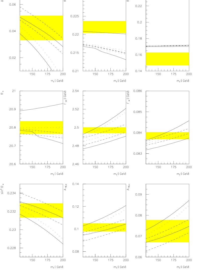
The main results in view of the recent precision data are:
$\bullet$ $R_{c}$ can hardly be moved towards the measured range.
$\bullet$ $R_{b}$ can come closer to the measured value, in particular for light $\tilde{t}_{R}$ and light charginos.
$\bullet$ $\alpha_{s}$ turns out to be smaller than in the minimal model because of the reasons explained in the beginning of this section.
$\bullet$ There are strong constraints from the other precision observables which forbid parameter configurations shifting $R_{b}$ into the observed $1\sigma$ range.

For obtaining the optimized SUSY parameter set, therefore, a global fit to all the electroweak precision data (including the top mass measurements) has to be performed, as done in refs. [127, 129]. Figure 10 displays the experimental data normalized to the best fit results in the SM and MSSM, with the data from this conference [129]. For the SM, $\alpha_{s}$ identified with the experimental number, therefore the corresponding result in Figure 6 is centered at 1. The most relevant conclusions are:
(i) The difference between the experimental and theoretical value of $R_{b}$ is diminished by a factor $\simeq 1/2$,
(ii) the central value for the strong coupling is $\alpha_{s}=0.110$ and thus is very close to the value obtained from deep inelastic scattering,
(iii) the other observables are practically unchanged,
(iv) the $\chi^{2}$ of the fit is slightly better than in the minimal model.

Figure 10: Experimental data normalized to the best fit results in the SM and MSSM.

10 Conclusions

The experimental data for testing the electroweak theory have achieved an impressive accuracy. For the interpretation of the precision experiments radiative corrections, or quantum effects, play a crucial role. The calculation of radiative corrections is theoretically well established, and many contributions have become available over the past few years to improve and stabilize the Standard Model predictions. After taking the measured $Z$ mass, besides $\alpha$ and $G_{\mu}$, for completion of the input, each other precision observable provides a test of the electroweak theory. The theoretical predictions of the Standard Model depend on the mass of the recently discovered top quark and of the as yet experimentally unknown Higgs boson through the virtual presence of these particles in the loops. As a consequence, precision data can be used to pin down the allowed range of the mass parameters, yielding $m_{t}$ in beautiful agreement with the directly measured value.

Theoretical uncertainties in the Standard Model predictions have their origin essentially in the uncertainties of the hadronic vacuum polarization of the photon and from the unknown higher order contributions. In order to reach a theoretical accuracy at the level 0.1% or below, new experimental data on $\Delta\alpha$ and more complete electroweak 2-loop calculations are required. The observed deviations of several $\sigma$’s in $R_{b},R_{c},A_{LR}$ reduce the quality of the Standard Model fits significantly, but the indirect determination of $m_{t}$ is remarkably stable. Still impressive is the perfect agreement between theory and experiment for the whole set of the other precision observables. Supersymmetry can improve the situtation due to an enhancement of $R_{b}$ by new particles in the range of 100 GeV or even below, but it is not possible to accomodate $R_{c}$. Within the MSSM analysis, the value for $\alpha_{s}$ is close to the one from deep-inelastic scattering.

References

-
[1]
S.L. Glashow, Nucl. Phys. B22 (1961) 579;
S. Weinberg, Phys. Rev. Lett. 19 (1967) 1264;
A. Salam, in: Proceedings of the 8th Nobel Symposium, p. 367, ed. N. Svartholm, Almqvist and Wiksell, Stockholm 1968 - [2] S.L. Glashow, I. Iliopoulos, L. Maiani, Phys. Rev. D2 (1970) 1285;
[3]
N. Cabibbo, Phys. Rev. Lett. 10 (1963) 531;
M. Kobayashi, K. Maskawa, Prog. Theor. Phys. 49 (1973) 652 -
[4]
H.Y. Han, Y. Nambu, Phys. Rev. 139 (1965) 1006;
C. Bouchiat, I. Iliopoulos, Ph. Meyer, Phys. Lett. B138 (1972) 652 - [5] G. ’t Hooft, Nucl. Phys. B33 (1971) 173; Nucl. Phys. B35 (1971) 167
[6]
The LEP Collaborations ALEPH, DELPHI,L3, OPAL and the LEP Electroweak
Working Group, CERN-PPE/95-172;
A. Olshevsky, talk at the International Europhysics Conference on High Energy Physics, Brussels 1995 (to appear in the Proceedings);
P. Renton, talk at the 17th International Symposium on Lepton-Photon Interactions, Beijing 1995, Oxford OUN-95-20 (to appear in the Proceedings) -
[7]
UA2 Collaboration, J. Alitti et al.,
Phys. Lett. B276 (1992) 354;
CDF Collaboration, F. Abe et al., Phys. Rev. D43 (1991) 2070;
D0 Collaboration, C.K. Jung, talk at the 27th International Conference on High Energy Physics, Glasgow 1994;
CDF Collaboration, F. Abe et al., FERMILAB-PUB-95/033-E; FERMILAB-PUB-95/035-E (1995) -
[8]
CDF Collaboration, F. Abe et al., Phys. Rev. Lett. 74 (1995) 2626;
D0 Collaboration, S. Abachi et al., Phys. Rev. Lett. 74 (1995) 2632 - [9] L.D. Faddeev, V.N. Popov, Phys. Lett. B25 (1967) 29
- [10] M. Böhm, W. Hollik, H. Spiesberger, Fortschr. Phys. 34 (1986) 687
- [11] A. Denner, T. Sack, Nucl. Phys. B347 (1990) 203
- [12] G. Passarino, in: Proceeedings of the LP-HEP 91 Conference, Geneva 1991, eds. S. Hegarty, K. Potter, E. Quercigh, World Scientific, Singapore 1992
[13]
G. Passarino, Nucl. Phys. B361 (1991) 351;
G. Passarino, in Proceedings of the XXVIth Rencontre de Moriond: ’91 Electroweak Interactions and Unified Theories, ed. Tran Thanh Van - [14] G. ’t Hooft, Nucl. Phys. B61 (1973) 455; Nucl. Phys. B62 (1973) 444
- [15] D.A. Ross, J.C. Taylor, Nucl. Phys. B51 (1973) 25
- [16] G. Passarino, M. Veltman, Nucl. Phys. B160 (1979) 151
- [17] M. Consoli, Nucl. Phys. B160 (1979) 208
[18]
A. Sirlin, Phys. Rev. D22 (1980) 971;
W. J. Marciano, A. Sirlin, Phys. Rev. D22 (1980) 2695;
A. Sirlin, W. J. Marciano, Nucl. Phys. B189 (1981) 442 -
[19]
D.Yu. Bardin, P.Ch. Christova, O.M. Fedorenko,
Nucl. Phys. B175 (1980) 435; Nucl. Phys. B197 (1982) 1;
D.Yu. Bardin, M.S. Bilenky, G.V. Mithselmakher, T. Riemann, M. Sachwitz, Z. Phys. C44 (1989) 493 - [20] J. Fleischer, F. Jegerlehner, Phys. Rev. D23 (1981) 2001
[21]
K.I. Aoki, Z. Hioki, R. Kawabe, M. Konuma, T. Muta,
Suppl. Prog. Theor. Phys. 73 (1982) 1;
Z. Hioki, Phys. Rev. Lett. 65 (1990) 683, E:1692; Z. Phys. C49 (1991) 287 - [22] M. Consoli, S. LoPresti, L. Maiani, Nucl. Phys. B223 (1983) 474
- [23] D.Yu. Bardin, M.S. Bilenky, G.V. Mithselmakher, T. Riemann, M. Sachwitz, Z. Phys. C44 (1989) 493
- [24] W. Hollik, Fortschr. Phys. 38 (1990) 165
- [25] M. Consoli, W. Hollik, F. Jegerlehner, in: Physics at LEP 1, eds. G. Altarelli, R. Kleiss and C. Verzegnassi, CERN 89-08 (1989)
[26]
G. Passarino, R. Pittau, Phys. Lett. B228 (1989) 89;
V.A. Novikov, L.B. Okun, M.I. Vysotsky, CERN-TH.6538/92 (1992) -
[27]
M. Veltman, Phys. Lett. B91 (1980) 95;
M. Green, M. Veltman, Nucl. Phys. B169 (1980) 137, E: Nucl. Phys. B175 (1980) 547;
F. Antonelli, M. Consoli, G. Corbo, Phys. Lett. B91 (1980) 90;
F. Antonelli, M. Consoli, G. Corbo, O. Pellegrino, Nucl. Phys. B183 (1981) 195 - [28] G. Passarino, M. Veltman, Phys. Lett. B237 (1990) 537
[29]
W.J. Marciano, A. Sirlin, Phys. Rev. Lett. 46 (1981) 163;
A. Sirlin, Phys. Lett. B232 (1989) 123 - [30] G. Degrassi, S. Fanchiotti, A. Sirlin, Nucl. Phys. B351 (1991) 49
- [31] G. Degrassi, A. Sirlin, Nucl. Phys. B352 (1991) 342
- [32] D.C. Kennedy, B.W. Lynn, Nucl. Phys. B322 (1989) 1
- [33] M. Kuroda, G. Moultaka, D. Schildknecht, Nucl. Phys. B350 (1991) 25
- [34] J.C. Ward, Phys. Rev. 78 (1950) 1824
- [35] G. ’t Hooft, M. Veltman, Nucl. Phys. B135 (1979) 365
[36]
C. Bollini, J. Giambiagi Nuovo Cim. 12B (1972) 20;
J. Ashmore, Nuovo Cim. Lett. 4 (1972) 289;
G. ’t Hooft, M. Veltman, Nucl. Phys. B44 (1972) 189 - [37] P. Breitenlohner, D. Maison, Comm. Math. Phys. 52 (1977) 11, 39, 55
[38]
M. Veltman, Nucl. Phys. B123 (1977) 89;
M.S. Chanowitz, M.A. Furman, I. Hinchliffe, Phys. Lett. B78 (1978) 285 -
[39]
R.E Behrends, R.J. Finkelnstein, A. Sirlin,
Phys. Rev. 101 (1956) 866;
T. Kinoshita, A. Sirlin, Phys. Rev. 113 (1959) 1652 - [40] S. Eidelman, F. Jegerlehner, Z. Phys. C67 (1995) 585
- [41] H. Burkhardt, B. Pietrzyk, Phys. Lett. B356 (1995) 398
- [42] F. Jegerlehner, Progress in Particle and Nuclear Physics 27 (1991) 1, updated from: H. Burkhardt, F. Jegerlehner, G. Penso, C. Verzegnassi, Z. Phys. C43 (1989) 497;
- [43] M.L. Swartz, preprint SLAC-PUB-95-7001 (1995)
- [44] A.D. Martin, D. Zeppenfeld, Phys. Lett. B345 (1995) 558
- [45] M. Veltman, Acta Phys. Polon. B8 (1977) 475.
- [46] W.J. Marciano, Phys. Rev. D20 (1979) 274
- [47] M. Consoli, W. Hollik, F. Jegerlehner, Phys. Lett. B227 (1989) 167.
- [48] J.J. van der Bij, F. Hoogeveen, Nucl. Phys. B283 (1987) 477
[49]
R. Barbieri, M. Beccaria, P. Ciafaloni, G. Curci, A. Vicere,
Phys. Lett. B288 (1992) 95; Nucl. Phys. B409 (1993) 105;
J. Fleischer, F. Jegerlehner, O.V. Tarasov, Phys. Lett. B319 (1993) 249 - [50] A. Djouadi, C. Verzegnassi, Phys. Lett. B195 (1987) 265
[51]
L. Avdeev, J. Fleischer, S. M. Mikhailov, O. Tarasov,
Phys. Lett. B336 (1994) 560;
E: Phys. Lett. B349 (1995) 597;
K.G. Chetyrkin, J.H. Kühn, M. Steinhauser, Phys. Lett. B351 (1995) 331 -
[52]
A. Djouadi, Nuovo Cim. 100A (1988) 357;
D. Yu. Bardin, A.V. Chizhov, Dubna preprint E2-89-525 (1989);
B.A. Kniehl, Nucl. Phys. B347 (1990) 86;
F. Halzen, B.A. Kniehl, Nucl. Phys. B353 (1991) 567;
A. Djouadi, P. Gambino, Phys. Rev. D49 (1994) 3499 -
[53]
B.A. Kniehl, J.H. Kühn, R.G. Stuart, Phys. Lett. B214 (1988) 621;
B.A. Kniehl, A. Sirlin, Nucl. Phys. B371 (1992) 141; Phys. Rev. D47 (1993) 883;
S. Fanchiotti, B.A. Kniehl, A. Sirlin, Phys. Rev. D48 (1993) 307 - [54] K.G. Chetyrkin, J.H. Kühn, M. Steinhauser, preprint KA-TTP95-13 (1995)
- [55] A. Sirlin, Phys. Rev. D29 (1984) 89
- [56] S. Fanchiotti, A. Sirlin, New York University preprint NYU-Th-91/02/04 (1991), in: Beg Memorial Volume, eds. A. Ali and P. Hoodbhoy, World Scientific, Singapore 1991
[57]
G.L. Fogli and D. Haidt, Z. Phys. C40 (1988) 379;
CDHS Collaboration, H. Abramowicz et al., Phys. Rev. Lett. B57 (1986) 298; A. Blondel et al, Z. Phys. C45 (1990) 361;
CHARM Collaboration, J.V. Allaby et al., Phys. Lett. B177 (1987) 446;
Z. Phys. C36 (1987) 611;
CHARM-II Collaboration, D. Geiregat et al., Phys. Lett. B247 (1990) 131;
Phys. Lett. B259 (1991) 499;
CCFR Collaboration, C.G. Arroyo et al., Phys. Rev. Lett. 72 (1994) 3452;
D. Harris (CCFR Collaboration), talk at the International Europhysics Conference on High Energy Physics, Brussels 1995 (to appear in the Proceedings) - [58] C.H. Llewellyn Smith, Nucl. Phys. B228 (1983) 205
[59]
A.A. Akhundov, D.Yu. Bardin, T. Riemann, Nucl. Phys. B276 (1986) 1;
W. Beenakker, W. Hollik, Z. Phys. C40 (1988) 141;
J. Bernabeu, A. Pich, A. Santamaria, Phys. Lett. B200 (1988) 569; Nucl. Phys. B363 (1991) 326 - [60] P. Langacker, M. Luo, Phys. Rev. D44 (1991) 817
[61]
U. Amaldi, W. de Boer, H. Fürstenau, Phys. Lett. B260 (1991) 447;
J. Ellis, S. Kelley, D.V. Nanopoulos, Phys. Lett. B260 (1991) 131; Phys. Lett. B287 (1992) 725;
G.G. Ross, R.G. Roberts, Nucl. Phys. B377 (1992) 571 - [62] A. Denner, W. Hollik, B. Lampe, Z. Phys. C60 (1993) 93
[63]
J. Fleischer, O.V. Tarasov, F. Jegerlehner,
P. Ra̧czka,
Phys. Lett. B293 (1992) 437;
G. Buchalla, A.J. Buras, Nucl. Phys. B398 (1993) 285;
G. Degrassi, Nucl. Phys. B407 (1993) 271;
K.G. Chetyrkin, A. Kwiatkowski, M. Steinhauser, Mod. Phys. Lett. A8 (1993) 2785 -
[64]
A. Kwiatkowski, M. Steinhauser, Phys. Lett. B344 (1995) 359;
S. Peris, A. Santamaria, CERN-TH-95-21 (1995) -
[65]
F.A. Berends et al.,
in:
Z Physics at LEP 1, CERN 89-08 (1989), eds. G. Altarelli, R. Kleiss, C. Verzegnassi, Vol. I, p. 89;
W. Beenakker, F.A. Berends, S.C. van der Marck, Z. Phys. C46 (1990) 687 - [66] A. Borelli, M. Consoli, L. Maiani, R. Sisto, Nucl. Phys. B333 (1990) 357
- [67] G. Burgers, F.A. Berends, W. Hollik, W.L. van Neerven, Phys. Lett. B203 (1988) 177
- [68] D. Yu. Bardin, A. Leike, T. Riemann, M. Sachwitz, Phys. Lett. B206 (1988) 539
[69]
G. Valencia, S. Willenbrock, Phys. Lett. B 259 (1991) 373;
R.G. Stuart, Phys. Lett. B272 (1991) 353 - [70] G. Burgers, F.A. Berends, W.L.van Neerven, Nucl. Phys. B297 (1988) 429; E: Nucl. Phys. B304 (1988) 921
- [71] W. Beenakker, F.A. Berends, S.C. van der Marck, Z. Phys. C46 (1990) 687
[72]
K.G. Chetyrkin, A.L. Kataev, F.V. Tkachov, Phys. Lett. B85 (1979) 277;
M. Dine, J. Sapirstein, Phys. Rev. Lett. 43 (1979) 668;
W. Celmaster, R. Gonsalves, Phys. Rev. Lett. 44 (1980) 560;
S.G. Gorishny, A.L. Kataev, S.A. Larin, Phys. Lett. B259 (1991) 144;
L.R. Surguladze, M.A. Samuel, Phys. Rev. Lett. 66 (1991) 560;
A. Kataev, Phys. Lett. B287 (1992 209 -
[73]
T.H. Chang, K.J.F Gaemers, W.L. van Neerven, Nucl. Phys. B202 (1982) 407;
J.H. Kühn, B.A. Kniehl, Phys. Lett. B224 (1990) 229;
Nucl. Phys. B329 (1990) 547;
K.G. Chetyrkin, J.H. Kühn, Phys. Lett. B248 (1992) 359;
K.G. Chetyrkin, J.H. Kühn, A. Kwiatkowski, Phys. Lett. B282 (1992) 221;
K.G. Chetyrkin, A. Kwiatkowski, Phys. Lett. B305 (1993) 285; Karlsruhe preprint TTP93-24 (1993);
K.G. Chetyrkin, Karlsruhe preprint TTP93-5 (1993);
K.G. Chetyrkin, J.H. Kühn, A. Kwiatkowski, in [91], p. 175;
S. Larin, T. van Ritbergen, J.A.M. Vermaseren, ibidem, p. 265; Phys. Lett. B320 (1994) 159 - [74] A. Hoang, J.H. Kühn, T. Teubner, Nucl. Phys. B455 (1995) 3; B452 (1995) 173
- [75] M. Böhm, W. Hollik Nucl. Phys. B204 (1982) 45; Z. Phys. C 23 (1984) 31
[76]
S. Jadach, J.H. Kühn, R.G. Stuart,
Z. Wa̧s, Z. Phys. C38 (1988) 609;
J.H. Kühn, R.G. Stuart, Phys. Lett. B200 (1988) 360 - [77] D. Bardin, M.S. Bilenky, O.M. Fedorenko, T. Riemann, Dubna preprint JINR-E2-88-324 (1988)
- [78] D. Bardin, M.S. Bilenky, A. Chizhov, A. Sazonov, Yu. Sedykh, T. Riemann, M. Sachwitz, Phys. Lett. B229 (1989) 405
- [79] J. Jersak, E. Laerman, P.M. Zerwas, Phys. Rev. D25 (1980) 1218
- [80] A. Djouadi, Z. Phys. C39 (1988) 561
- [81] A. Djouadi, B. Lampe, P. Zerwas, Z. Phys. C67 (1995) 123
[82]
M. Böhm, W. Hollik et al.,
Z Physics at LEP 1, CERN 89-08 (1989), eds. G. Altarelli, R. Kleiss, C. Verzegnassi, Vol. I, p. 203;
W. Beenakker, F.A. Berends, S.C. van der Marck, Phys. Lett. B252 (1990) 299 - [83] J.H. Kühn, P.Zerwas et al., in: Z Physics at LEP 1, CERN 89-08 (1989), eds. G. Altarelli, R. Kleiss, C. Verzegnassi, Vol. I, p. 267
- [84] D. Bardin, M.S. Bilenky, A. Chizhov, A. Sazonov, O. Fedorenko, T. Riemann, M. Sachwitz, Nucl. Phys. B351 (1991) 1
- [85] W. Beenakker, F.A. Berends, W.L. van Neerven, in: Proceedings of the 1989 Ringberg Workshop Radiative Corrections for Collisions, p. 3, ed. J.H. Kühn, Springer, Berlin - Heidelberg - New York 1989
- [86] D. Bardin, L. Vertogradov, Yu. Sedykh, T. Riemann, CERN-TH.5434/89 (1989)
- [87] D. Bardin et al., CERN-TH.6443/92 (1992)
- [88] G. Montagna, F. Piccinini, O. Nicrosini, G. Passarino, R. Pittau, Pavia-Torino preprint FNT/T-92/02, DFTT/G-93-1 (1993)
- [89] B.A. Kniehl, in [91], p. 299
- [90] D. Bardin et al., in [91], p. 7
- [91] Reports of the Working Group on Precision Calculations for the Resonance, CERN 95-03 (1995), eds. D. Bardin, W. Hollik, G. Passarino
- [92] D. Bardin, talk at the International Europhysics Conference on High Energy Physics, Brussels 1995 (to appear in the Proceedings)
- [93] G. Degrassi, S. Fanchiotti, F. Feruglio, P. Gambino, A. Vicini, in [91], p. 163
- [94] S. Bethke, in: Proceedings of the Tennessee International Symposium on Radiative Corrections, Gatlinburg 1994, Ed. B.F.L. Ward, World Scientific 1995
- [95] SLD Collaboration, K. Abe et al., Phys. Rev. Lett. 73 (1994) 25; M. Woods (SLD Collaboration), talk at the International Europhysics Conference on High Energy Physics, Brussels 1995 (to appear in the Proceedings)
- [96] CHARM II Collaboration, P. Vilain et al., Phys. Lett. B335 (1994) 246; B345 (1995) 115
- [97] S. Sarantakos, A. Sirlin, Nucl. Phys. B217 (1983) 84; D.Yu. Bardin V.A. Dokuchaeva, Nucl. Phys. B246 (1984) 221; M. Böhm, W. Hollik, H. Spiesberger, Z. Phys. C27 (1985) 523
- [98] J.-F. Grivaz, talk at the International Europhysics Conference on High Energy Physics, Brussels 1995 (to appear in the Proceedings), LAL-95-83
[99]
J. Ellis, G.L. Fogli, E. Lisi, CERN-TH-95-202,
hep-ph/9507424;
P. Chankowski, S. Pokorski, hep-ph/9509207 - [100] M. Lindner, M. Sher, H. Zaglauer, Phys. Lett. B228 (1989) 139
- [101] Kuti et al., Phys. Rev. Lett. 61 (1988) 678; Hasenfratz et al., Nucl. Phys. B317 (1989) 81; M. Lüscher, P. Weisz, Nucl. Phys. B318 (1989) 705
- [102] A. Ghinculov, Nucl. Phys. B455 (1995) 21
- [103] M. Carena. P. Zerwas (conveners) et al., report on Higgs Physics, hep-ph/9602250, to appear in the Proceedings of the LEP2 Workshop, eds. G. Altarelli, T, Sjöstrand, F. Zwirner
- [104] G. Burgers, F. Jegerlehner, in: Physics at LEP 1, eds. G. Altarelli, R. Kleiss and C. Verzegnassi, CERN 89-08 (1989)
- [105] M.E. Peskin, T. Takeuchi, Phys. Rev. Lett. 65 (1990) 964
[106]
G. Altarelli, R. Barbieri, Phys. Lett. B253 (1991) 161;
G. Altarelli, R. Barbieri, S. Jadach, Nucl. Phys. B269 (1992) 3; E: Nucl. Phys. B276 (1992) 444 - [107] D.C. Kennedy, P. Langacker, Phys. Rev. Lett. 65 (1990) 2967
- [108] W.J. Marciano, J.L. Rosner, Phys. Rev. Lett. 65 (1990) 2963
- [109] B.W. Lynn, M.E. Peskin, R.G. Stuart, in: Physics with LEP, eds. J. Ellis and R. Peccei, CERN 86-02 (1986)
[110]
R. Barbieri, M.Frigeni, F. Caravaglios, Phys. Lett. B279 (1992) 169;
V.A. Novikov, L.B. Okun, M.I. Vysotsky, CERN-TH.6943/93 (1993);
M. Bilenky, K. Kolodziej, M. Kuroda, D. Schildknecht, Phys. Lett. B319 (1993) 319;
S. Dittmaier, D. Schildknecht, M. Kuroda, Nucl. Phys. B448 (1995) 3 -
[111]
B. Holdom, J. Terning, Phys. Lett. B247 (1990) 88;
M. Golden, L. Randall, Nucl. Phys. B361 (1991) 3;
C. Roiesnel, T.N. Truong, Phys. Lett. B256 (1991) 439 - [112] G. Altarelli, R. Barbieri, F. Caravaglios, Nucl. Phys. B405 (1993) 3; CERN-TH.6895/93 (1993)
- [113] F. Caravaglios, talk at the International Europhysics Conference on High Energy Physics, Brussels 1995 (to appear in the Proceedings)
[114]
D. Toussaint, Phys. Rev. D18 (1978) 1626;
J.M Frere, J. Vermaseren, Z. Phys. C19 (1983) 63 -
[115]
S. Bertolini, Nucl. Phys. B272 (1986) 77;
W. Hollik, Z. Phys. C32 (1986) 291; Z. Phys. C37 (1988) 569 - [116] A. Denner, R. Guth, J.H. Kühn, Phys. Lett. B240 (1990) 438
- [117] A. Denner, R. Guth, W. Hollik, J.H. Kühn, Z. Phys. C51 (1991) 695
- [118] B.W. Lynn, E. Nardi, Nucl. Phys. B381 (1992) 467
- [119] T. Blank, Diploma thesis, Univ. Karlsruhe 1995
[120]
G. Altarelli et al.,
Nucl. Phys. B342 (1990) 15; Phys. Lett. B245 (1990) 669;
M.C. Gonzalez-Garcia, J.W.F. Valle, Phys. Lett. B259 (1991) 365;
J. Layssac, F.M. Renard, C. Verzegnassi, Z. Phys. C53 (1992) 97 - [121] F. del Aguila, W. Hollik, J.M. Moreno, M. Quiros, Nucl. Phys. B372 (1992) 3
[122]
P. Chiapetta, J. Layssac, F.M. Renard,
C. Verzegnassi, PM/96-05, hep-ph/9602306;
G. Altarelli, N. Di Bartolomeo,F. Feruglio, R, Gatto, M. Mangano, CERN-TH/96-20, hep-ph/9601324 -
[123]
A. Denner, R. Guth, W. Hollik, J.H. Kühn,
Z. Phys. C51 (1991) 695;
J. Rosiek, Phys. Lett. B252 (1990) 135;
F. Cornet, W. Hollik, W. Mösle, Nucl. Phys. B428 (1994) 61;
M. Boulware, D. Finnell, Phys. Rev. D44 (1991) 2054 -
[124]
G. Altarelli, R. Barbieri, F. Caravaglios,
CERN-TH.7536/94 (1994);
C.S. Lee, B.Q. Hu, J.H. Yang, Z.Y. Fang, J. Phys. G19 (1993) 13;
Q. Hu, J.M. Yang, C.S. Li, Comm. Theor. Phys. 20 (1993) 213;
J.D. Wells, C. Kolda, G.L. Kane, Phys. Lett. B338 (1994) 219;
G.L. Kane, R.G. Stuart, J.D. Wells, Phys. Lett. B354 (1995) 350 -
[125]
P. Chankowski, A. Dabelstein, W. Hollik, W. Mösle,
S. Pokorski, J. Rosiek, Nucl. Phys. B417 (1994) 101;
D. Garcia, J. Solà, Mod. Phys. Lett. A9 (1994) 211 -
[126]
D. Garcia, R. Jiménez, J. Solà,
Phys. Lett. B347 (1995) 309; B347 (1995) 321;
D. Garcia, J. Solà, Phys. Lett. B357 (1995) 349 -
[127]
P. Chankowski, S. Pokorski, preprint
IFT-UW-95/5 (1995);
P. Chankowski, talk at the International Europhysics Conference on High Energy Physics, Brussels 1995 (to appear in the Proceedings) - [128] A. Dabelstein, W. Hollik, W. Mösle, preprint KA-TP-5-1995 (1995), Proceedings of the Ringberg Workshop “Perspectives for Electroweak Interactions in Collisions”, Ringberg Castle, February 1995, Ed. B.A. Kniehl, World Scientific 1995 (p. 345)
[129]
W. De Boer, S. Meyer, A. Dabelstein, W. Hollik,
W. Mösle, U. Schwickerath (to be published);
W. Hollik, talk at the International Europhysics Conference on High Energy Physics, Brussels 1995 (to appear in the Proceedings)