Abstract

The structure functions $F^{L}_{1}$ and $F^{L}_{2}$ of longitudinal virtual photon at low virtualities are calculated in the framework of chiral pertubation theory(ChPT) in the zero and first order of ChPT. It is assumed that the virtuality of target longitudinal photon $p^{2}$ is much less than the virtuality of the hard projectile photon $Q^{2}$ and both are less than the characteristic ChPT scale. In this approximation the structure functions are determined by the production of two pions in $\gamma\gamma$ collisions. The numerical results for $F^{L}_{2}$ and $F^{L}_{1}$ are presented (the upper index refers to longitudinal polarization of the virtual target photon). The possibilities of measurements of these structure functions are briefly discussed.

1 Introduction

    As was mentioned in Ref’s[1,2] the structure function of longitudinal virtual photon $F_{2}^{L}(x,p^{2})$ in massless QCD is nonvanishing, when photon virtuality $p^{2}$ is going to zero. This unusual circumstance is caused by the fact that the imaginary part of the forward $\gamma\gamma$ scattering amplitude (box diagrams with quarks in the loops), determining the photon structure function , has a pole $1/p^{2}$ in the virtuality of the target photon. After multiplication by the product of longitudinal photon polarizations in the initial and final states, proportional to $p^{2}$ $(e^{L}_{i}e^{L}_{f}\propto p^{2})$, this results in nonvanishing $F_{2}^{L}(x,p^{2})$ at $p^{2}\rightarrow 0$.

The seemingly nonvanishing interaction of longitudinal photons at $p^{2}\rightarrow 0$ in massless theories does not result[3,4] in any inconsistency of the theory: the arising problems in the gedanken experiments with longitudinal photons are solved by exploiting the concept of the formation zone[3]. There are nonpertubative effects which are important for determination of the longitudinal photon structure function $F_{2}^{L}(x,p^{2})$ at low $p^{2}$. For this reason it is impossible to find it basing on QCD now. Even the approach, using the operator product expansion in $1/p^{2}$ and the analytical continuation in the domain of low $p^{2}$, which was succeful in the determination of structure function of real and virtual transverse photon[2,5] is not working here: the extrapolation to low $p^{2}$ appears to be impossible.

At low virtualities and energies of all initial and final particles in the given process QCD is equivalent to the ChPT: the theory of almost massless particles - pions (for reviwes see[6-8]). Therefore we may expect that the peculiar properties of longitudinal photon in massless QCD will manifest themselves in ChPT with massless pions. This idea was proposed in Ref.[1].

The goal of this paper is to perform the quantitave calculations of the longitudinal photon structure functions at low $p^{2}$ basing on ChPT. In order to be in the framework of ChPT it is necessary to assume that not only virtuality of target (soft) photon $p^{2}$ is less than the applicability limit of ChPT $M^{2}\approx m_{\rho}^{2}=0.6$GeV², but also that the virtuality of the probe (hard) photon $Q^{2}=-q^{2}$ in $\gamma\gamma$ scattering is below this limit. It means that the photon structure functions are not in the scaling region of $Q^{2}$.

There is the essential difference in the photon structure functions at high and low virtualities $Q^{2}$ of probe (hard) photon. At high $Q^{2}$ the structure functions which are transverse in the polarization of the hard photon are dominating for the case of longitudinal, as well as for transverse polarized soft photon. This is a direct consequence of the fact that at high $Q^{2}$ the $\gamma\gamma$ scattering proceeds through the $\gamma$-scattering on quarks. At low $Q^{2}$ and $p^{2}$ the $\gamma\gamma$ scattering cross section is determined by the production of pions. It is known [9], that in the virtual photon scattering on free spinless boson the cross section of the longitudinally polarized photon is dominating. This means, that at low $Q^{2}$ and $p^{2}$ the longitudinal structure function will exceed the transverse one, $F_{L}\approx F_{2}/2x\gg F_{1}$.

In this paper the longitudinal virtual photon structure functions are calculated in the zero and first order in ChPT. The results are presented for structure functions $F^{L}_{L}(x,p^{2},Q^{2})$, $F^{L}_{2}(x,p^{2},Q^{2})$ and $F^{L}_{1}(x,p^{2},Q^{2})$, where the upper index refers to the polarization of the soft (target) photon with momentum $p$ and the lower index refers to the polarization of the hard (projectile) photon with momentum $q$, $-q^{2}=Q^{2}$.

The expansion parameter in ChPT is $M^{2}=C\pi^{2}F_{\pi}^{2}$, where $F_{\pi}=93$ Mev is the pion decay constant and $C$ is the constant depending on process and in this case it is about 6. Let us assume that $Q^{2}/M^{2}$, $p^{2}/M^{2}$ and $p^{2}/Q^{2}$ are the parameters of expansion and restrict ourselves by the first order terms in these ratios. For the value of $s=(p+q)^{2}$ the more weak limitation is imposed: $s\mathrel{\mathchoice{\lower 3.6pt\vbox{\halign{$\mathsurround=0pt\displaystyle\hfil#\hfil$\cr<\crcr\sim\crcr}}}{\lower 3.6pt\vbox{\halign{$\mathsurround=0pt\textstyle\hfil#\hfil$\cr<\crcr\sim\crcr}}}{\lower 3.6pt\vbox{\halign{$\mathsurround=0pt\scriptstyle\hfil#\hfil$\cr<\crcr\sim\crcr}}}{\lower 3.6pt\vbox{\halign{$\mathsurround=0pt\scriptscriptstyle\hfil#\hfil$\cr<\crcr\sim\crcr}}}}M^{2}$ because $s$ explicitly enters only in the small corrections to the results. The pion mass $\mu$ will be partly accounted: no assumption $|p^{2}|\gg\mu^{2}$ is used but corrections proportional to $\mu^{2}/Q^{2}$ and $\mu^{2}/s$ are neglected, besides the overall phase space factor.

In the section 2 the results of calculations of $F^{L}_{2}$, $F^{L}_{1}$ and $F^{L}_{L}$ in the zero order of ChPT are presented. In section 3 the first order terms in ChPT are calculated. In the section 4 the numerical results for the structure functions are given and the possibilities of the measurements of these structure functions are briefly discussed.

2 Calculation of the Structure Functions in the zero order of ChPT

    In order to get the structure function $F^{L}_{2}$ of the longitudinal target photon the imaginary part of $\gamma\gamma$ forward scattering amplitude $ImT_{\mu\nu\lambda\sigma}(p,q)$ must be multiplied by the product of longitudinal photon polarization in the initial and final states

$$e^{L}_{\lambda}(p)e^{L}_{\sigma}(p)=-\frac{p^{2}}{\nu^{2}-p^{2}q^{2}}(q_{\lambda}-\frac{\nu p_{\lambda}}{p^{2}})(q_{\sigma}-\frac{\nu p_{\sigma}}{p^{2}}),$$ (1)

where $\nu=pq$ and indeces $\mu,\nu$ and $\lambda,\sigma$ refer to hard and soft photon correspondingly. In the final answer the terms proportional to $p_{\mu}p_{\nu}$ must be separated

$$F^{L}_{2}(p^{2},q^{2},\nu)=2\alpha\nu\left\{ImT_{\mu\nu\lambda\sigma}(p,q)e^{L}_{\lambda}(p)e^{L}_{\sigma}(p)\right\}_{term\propto p_{\mu}p_{\nu}}$$ (2)

In the zero order of ChPT the proportional to $p_{\mu}p_{\nu}$ term of imaginary part of $\gamma\gamma$ forward scattering amplitude $ImT_{\mu\nu\lambda\sigma}(p,q)$ is determined by the two box diagrams Figs. 1a,b, corresponding to standard scalar electrodynamics. It is easy to see that the diagrams of Fig. 2, where two photon interact with two pions at one point - the diagrams arising from $A_{\mu}^{2}\phi^{+}\phi$ term in Lagrangian of scalar electrodynamics do not contribute to (2) because their contributions into imaginary part of amplitude have no terms proportional to $p_{\mu}p_{\nu}$. (The contributions of the second terms in the brackets in (1) vanish due to current conservation at the soft photon vertex.)

The imaginary part of the amplitude is connected with discontinuity of the amplitude in $s$ by:

$$ImT_{\mu\nu\lambda\sigma}(p^{2},q^{2},s)=\frac{1}{2i}[T_{\mu\nu\lambda\sigma}(p^{2},q^{2},s+i0)-T_{\mu\nu\lambda\sigma}(p^{2},q^{2},s-i0)].$$ (3)

The calculation of the diagrams of Fig.1 gives: for the direct diagram:

$$\begin{array}[]{ll}F^{L(fig.1a)}_{2}=\frac{\alpha\chi}{2\pi}(1-4x^{2}\frac{p^{2}}{Q^{2}})\left\{x(1-2x)^{2}\left[(1-\frac{\mu^{2}}{p^{2}x(1-x+xp^{2}/Q^{2})})^{-1}(1+4\frac{p^{2}}{Q^{2}}x(1-2x))+\right.\right.\\[14.22636pt] \left.\left.+\frac{p^{2}}{Q^{2}}(-1+8x(1-x)+2x(2-3x)L)\right]+2\frac{p^{2}}{Q^{2}}x(1-2x)[1+2x-6x^{2}-2x^{2}L]-\frac{4}{3}x\frac{p^{2}}{Q^{2}}\right\}\end{array}$$ (4)

and for the crossing diagram:

$$F^{L(fig.1b)}_{2}=-\frac{\alpha\chi}{2\pi}\frac{p^{2}}{Q^{2}}x\left\{(1-4x^{2})[-1+x(1-x)(6+2L)]+\frac{2}{3}\right\}.$$ (5)

Here $x=Q^{2}/2\nu$ is the Bjorken variable, $\chi$ accounts two pion phase space,

$$\chi=\left(1-\frac{4\mu^{2}x}{Q^{2}(1-x)+p^{2}x}\right)^{1/2},$$ (6)

$$L=ln\left[\frac{x^{2}}{Q^{2}}(-p^{2}+\frac{\mu^{2}}{x(1-x)})\right],$$ (7)

and only the first order terms in the ratio $p^{2}/Q^{2}$ are retained. As follows from (4) in the theory with massless pions ($\mu^{2}\rightarrow 0$) the direct diagram results in nonvanishing longitudinal photon structure function at $p^{2}\rightarrow 0$, i.e. for quasireal photon. In this aspect the situation in the ChPT resembles the situation in the massless QCD[1,2]. In the real world at $p^{2}\rightarrow 0$ $F^{L}_{2}$ is going to zero proportionally to $p^{2}$ starting from the values of $p^{2}$ of order $\mu^{2}/x(1-x)$. If $Q^{2}$ is less than $M^{2}$, as we suppose, in this region of $p^{2}$ the terms, proportional to $p^{2}/Q^{2}$ become of importance, as well as the terms of the first order in ChPT.

As is well known (see e.g. [9]), for any target the structure function $F_{2}$ is proportional to the sum of scattering cross sections $\sigma_{T}+\sigma_{L}$ of virtual transverse and longitudinal photons. If the scattering proceeds on free massless fermion only $\sigma_{T}$ survives, $\sigma_{L}$=0. For the scattering on free massless boson the situation is opposite: $\sigma_{T}=0$, $\sigma_{L}\neq 0$. Therefore, in the zero order in ChPT the nonvanising contribution to $F^{L}_{2}$ comes from the scattering of longitudinally polarized hard probe photon and it is reasonable to calculate also $F^{L}_{L}(p^{2},Q^{2},x)$ - the structure function, corresponding the case, where both photons are longitudinally polarized. The structure function $F^{L}_{L}$ is related to $F^{L}_{1}$ and $F^{L}_{2}$ by:

$$F^{L}_{L}=-F^{L}_{1}+(1+4p^{2}x^{2}/Q^{2})F^{L}_{2}/2x.$$ (8)

The structure function $F^{L}_{L}(p^{2},Q^{2},\nu)$ is expressed through the imaginary part of the forward $\gamma\gamma$-scattering amplitude by:

$$F^{L}_{L}(p^{2},q^{2},\nu)=2\alpha\left\{ImT_{\mu\nu\lambda\sigma}(p,q)e^{L}_{\lambda}(p)e^{L}_{\sigma}(p)e^{L}_{\mu}(q)e^{L}_{\nu}(q)\right\},$$ (9)

where $e^{L}_{\mu}(q)e^{L}_{\nu}(q)$ is given by (1) with substituion $\lambda\rightarrow\mu$, $\sigma\rightarrow\nu$ and $p\leftrightarrow q$. In the case of $F^{L}_{L},$ unlike $F^{L}_{2}$, the diagrams of fig.2 are also contributing.

Due to simple relation (8) between $F^{L}_{2}$, $F^{L}_{1}$ and $F^{L}_{L}$ only results for $F^{L}_{2}$ and $F^{L}_{1}$ will be represented. The results of the calculation for $F^{L}_{1}$ in the scalar electrodynamics are the following:

$$F^{L(scal.el.)}_{1}=\frac{\alpha\chi}{2\pi}\frac{p^{2}}{Q^{2}}x(1-x)(1-2x)^{2}(L+3)$$ (10)

As is seen from (10) in the $F^{L}_{1}$ there is not zero order term in the $p^{2}/Q^{2}$ expansion.

3 The First Order ChPT Correction to Longitudinal Photon Structure Functions

The general method of calculation of ChPT corrections is exposed in Ref’s[6-8]. We will mainly use the results of Gasser and Leutwyler[6] which are presented in the form most convenient for the present calculations.

From the general form of ChPT effective Lagrangian it can be easily shown that in the first order in ChPT only the two pions intermediate states can contribute to the imaginary part of the forward $\gamma\gamma$- scattering amplitude.

To calculate corrections to the structure functions $F^{L}_{L}$ and $F^{L}_{2}$ in the first order of ChPT one should consider the general expression for effective Lagrangian which contains all terms permited by chiral invariance in the order (momentum)⁴.

In the leading order of ChPT the effective Lagrangian has the form

$$L^{(2)}=\frac{1}{2}F^{2}(\nabla_{\mu}U^{T}\nabla_{\mu}U)$$ (11)

where $U$ is a four-component ($U=\{U^{0},U^{i}\}$) real $O(4)$ vector of unit length $U^{T}U=1$. The space components of U are expressed through the pion fiels, $U^{i}=\phi^{i}/F$. The ChPT expansion corresponds to the expansion in inverse powers of $F^{2}$. So, in the first order of ChPT

$$U^{0}=1-\frac{1}{2}U^{i}U^{i}$$ (12)

The covariant derivative $\nabla_{\mu}$ is defined by

$$\nabla_{\mu}U^{0}=\partial_{\mu}U^{0}$$ (13)

$$\nabla_{\mu}U^{i}=\partial_{\mu}U^{i}+A_{\mu}\epsilon^{i3l}U^{l},$$ (14)

where $A_{\mu}$ is the electromagnetic field. Expressing the real pionic fields $\phi^{1}$ and $\phi^{2}$ through the fields of charged pions $\phi^{+}$ and $\phi$

$$\phi^{1}=\frac{1}{\sqrt{2}}(\phi+\phi^{+})\quad\phi^{2}=\frac{1}{\sqrt{2}i}(\phi-\phi^{+})$$ (15)

and expanding (11) up to terms $\sim 1/F^{2}$, we have (only charged pion fields are retained)

$$L^{(2)}=L^{scal.elec.}+\frac{1}{2F^{2}}\{\partial_{\mu}(\phi^{+}\phi)\}^{2},$$ (16)

where $L^{scal.elec.}=(\partial_{\mu}\phi+iA_{\mu}\phi)^{+}(\partial_{\mu}\phi+iA_{\mu}\phi)-\mu^{2}\phi^{+}\phi$. Second term in $L^{(2)}$ corresponds to the four pion interaction and leads to appearance of the loop corrections to the structure functions which are proportional to $1/F^{2}$.

In the order (momentum)⁴, i.e. $\sim 1/F^{2}$, there are two terms in the general effective Lagrangian of ChPT[6], which are essential for us

$$L_{5}=l_{5}(U^{T}{\cal F_{\mu\nu}F_{\mu\nu}}U)$$ (17)

$$L_{6}=l_{6}(\nabla_{\mu}U^{T}{\cal F_{\mu\nu}}\nabla_{\nu}U),$$ (18)

where

$$({\cal F_{\mu\nu}}U)^{i}=[(\nabla_{\mu}\nabla_{\nu}-\nabla_{\nu}\nabla_{\mu})U]^{i}.$$ (19)

In terms of charged pionic fields

$$L_{5}=\frac{-2l_{5}}{F^{2}}F_{\mu\nu}^{2}\phi^{+}\phi$$ (20)

$$L_{6}=\frac{-2il_{6}}{F^{2}}F_{\mu\nu}\{\partial_{\mu}\phi\partial_{\nu}\phi^{+}+iA_{\mu}\partial_{\nu}(\phi^{+}\phi)\},$$ (21)

where $F_{\mu\nu}$ is the electromagnetic field strength. Therefore in this order the effective chiral Lagrangian is given by

$$L=L^{scal.elec.}+\frac{1}{2F^{2}}\{\partial_{\mu}(\phi^{+}\phi)\}^{2}+L_{5}+L_{6},$$ (22)

where $L_{5}$ and $L_{6}$ are expressed in the terms of $\phi$, $\phi^{+}$ and $A_{\mu}.$ $L_{5}$ and $L_{6}$ serve as the counter terms for the renormalization of loops: the infinities arising in loop calculations are absorbed in $l_{5}$ and $l_{6}$, and as a result the finite values $\bar{l_{5}}$ and $\bar{l_{6}}$ arise.

For the calculation of the first order ChPT corrections to the structure functions we should calculate effective $\gamma\pi\pi$ and $\gamma\gamma\pi\pi$ vertices, substitute ones in all zero order diagrams of ChPT and collect terms proportional to $1/F^{2}$.

At first let us consider effective $\gamma\pi\pi$ vertex. In the chosen parameterization of U there are three diagrams which contribute to this vertex in the first order of ChPT (Fig.3). First diagram corresponds to vertex of $\gamma\pi\pi$ interaction in the scalar electrodynamics, the second comes from $L_{6}$ and the third is the loop (unitary) diagram. To renormalize the loop diagram it is convenient to use the dimensional regularization. The contribution of this diagram to the $\gamma\gamma\pi$ vertex can be divided into finite part and divergent part which contains the infinite factor $\lambda$, where $\lambda$ is :

$$\lambda=\frac{2}{4-d}+ln4\pi+1-\gamma_{E}-ln\frac{\mu^{2}}{\rho^{2}},$$

and $\rho$ is the scale of mass introduced by dimensional regularization.

In the sum of the diagrams the divergent part will be absorbed into $l_{6}$ and the following result for effective $\gamma\pi\pi$ vertex in the first order of ChPT was obtained[6]:

$$-\frac{1}{i}\Gamma_{\mu}(k,k^{\prime};q)=(k^{\prime}+k)_{\mu}-\frac{\left(\bar{l}_{6}-1/3+\sigma^{2}\{\sigma ln(\frac{\sigma-1}{\sigma+1})+2\}\right)}{48\pi^{2}F^{2}}(q_{\mu}kq-k_{\mu}q^{2}),$$ (23)

where

$$\sigma=(1-4\mu^{2}/q^{2})^{1/2},$$ (24)

$k$ and $k^{\prime}$ are the pion initial and final momenta, q is the photon momentum, $k=k^{\prime}+q.$ The numerical value of $\bar{l_{6}}$ was found in Ref. [6] from the data on electromagnetic charge radius of the pion:

$$\bar{l_{6}}=16.5\pm 1.1$$ (25)

After substuting this effective vertex in zero order diagrams in all cases the following combination appears

$$R_{6}(r^{2})=\bar{l}_{6}-1/3+\sigma^{2}(r^{2})\left\{\sigma(r^{2})ln\left[\frac{\sigma(r^{2})-1}{\sigma(r^{2})+1}\right]+2\right\}$$ (26)

where $r^{2}=q^{2}$ or $p^{2}$. The term proportional to $\sigma^{2}$ in (26) arises from the loop correction - the diagram Fig. 3c. It is much smaller numerically (about 10 times) than $\bar{l_{6}}$ and in what follows the difference between the values of $R_{6}(q^{2})$ and $R_{6}(p^{2})$ will be neglected.

In the case of $\gamma\gamma\pi\pi$ effective vertex there are six diagrams (fig. 4): first diagram comes from scalar electrodynamics, second and third ones correspond to $L_{6}$ and $L_{5}$, respectively, and the other diagrams are loop (unitary) corrections.

In principle we can write out the tensor structure of this vertex at once:

$$\frac{1}{i}\Gamma_{\mu\lambda}(p,q)=2\delta_{\mu\lambda}-\frac{R_{6}}{48\pi^{2}F^{2}}[q_{\lambda}(p+q)_{\mu}-\delta_{\mu\lambda}(p+q,q)+p_{\mu}(p+q)_{\lambda}-\delta_{\mu\lambda}(p+q,p)]+B(p_{\mu}q_{\lambda}-pq\delta_{\mu\lambda}).$$ (27)

This equation follows from the fact that total amplitude for $\gamma\gamma\pi\pi$ scattering must contain the factor $R_{6}$ multiplyed by tensor structure which is transverse in $q_{\mu}$ and $p_{\lambda}$ simultaneously. This conclusion can be checked by direct calculation.

To simplify the calculation of this vertex we multiply $\Gamma_{\mu\lambda}$ by $(p+q)_{\mu}(p+q)_{\lambda}$. After this procedure the term proportional to $R_{6}$ comes out. Taking into account that cutting pion propagators implies that these pions are on mass-shell and substituting vertex for four-pion interaction into diagrams 4(d-f), one can get the following expression for $B$

$$(B+\frac{8l_{5}}{F_{\pi}^{2}})(p^{2}q^{2}-\nu^{2})=\frac{(p+q)^{2}}{F^{2}}\frac{1}{i}\int\frac{d^{d}k}{(2\pi)^{d}}\frac{(p+q)^{2}+2k^{2}}{(k^{2}-\mu^{2})((k-p-q)^{2}-\mu^{2})}-$$

$$-\frac{1}{iF^{2}}\int\frac{d^{d}k}{(2\pi)^{d}}\frac{\left\{2(k,p+q)+q^{2}+\nu\right\}\left\{2(k,p+q)-p^{2}-\nu\right\}\left\{(p+q)^{2}+(k+q)^{2}+(k-p)^{2}\right\}}{\left(k^{2}-\mu^{2}\right)\left((k-p)^{2}-\mu^{2}\right)\left((k+q)^{2}-\mu^{2}\right)}$$ (28)

As usual, using dimensional regularization and absorbing the pole contributions, arising from the loop diagrams,by infinite constant $l_{5}$ we obtain the finite answer for B:

$$B=\frac{\bar{l_{5}}-1/3+\sigma^{2}(q^{2})\{\sigma(q^{2})ln(\frac{\sigma(q^{2})-1}{\sigma(q^{2})+1})+2\}+\delta}{24\pi^{2}F^{2}},$$ (29)

where

$$\delta=Re\left[\frac{3}{2}(1-2x)\int^{1}_{0}dz\int^{z}_{0}dy\frac{s}{\mu^{2}+y(1-y)Q^{2}-z(1-z)p^{2}-y(1-z)Q^{2}/x}-\right.$$

$$\left.-6(1-x)^{2}\left\{\sigma(s)ln(\frac{\sigma(s)-1}{\sigma(s)+1})-\sigma(q^{2})ln(\frac{\sigma(q^{2})-1}{\sigma(q^{2})+1})\right\}\right].$$ (30)

In the following the combination $\bar{l_{5}}-1/3+\sigma^{2}(q^{2})\left\{\sigma(q^{2})ln(\frac{\sigma(q^{2})-1}{\sigma(q^{2})+1})+2\right\}$ will be denoted as $R_{5}$. The numerical value of $\bar{l_{5}}$ was found in Ref.[6] from the data on $\pi\rightarrow e\nu\gamma$ decay:

$$\bar{l_{5}}=13.9\pm 1.3$$ (31)

The absolute value of $\delta$ does not exceed 3 and it is much less than $\bar{l_{5}}$ but the corrections due to $\bar{l_{5}}$ and $\bar{l_{6}}$ have a different sign and almost equal values and therefore the account of $\delta$ is necessary.

Substituting these effective vertices into all zero order diagrams and collecting the terms proportional to $1/F^{2}$ we get the final results for ChPT corrections to structure functions $F^{L}_{2}$ and $F^{L}_{1}$ of longitudinal photon:

$$F^{L(ChPT)}_{2}=\frac{R_{6}}{48\pi^{2}F^{2}}(-Q^{2}+p^{2})F^{L(fig.1a)}_{2}-\frac{R_{6}Q^{2}}{48\pi^{2}F^{2}}F^{L(fig.1b)}_{2}+$$

$$+\frac{\alpha\chi}{2\pi}\frac{R_{5}+\delta-R_{6}}{12\pi^{2}F^{2}}p^{2}x^{2}[4-4x+(1-2x)L]$$ (32)

and

$$F^{L(ChPT)}_{1}=-\frac{\alpha\chi}{2\pi}\frac{R_{6}p^{2}}{48\pi^{2}F^{2}}x(1-x)(1-2x)^{2}(L+3)$$ (33)

where $F^{L(fig.1a)}_{2}$ and $F^{L(fig.1b)}_{L}$ correspond to formulas (4) and (5).

4 Discussion

    Collecting all terms we can write final results for structure functions $F^{L}_{2}$:

$$F^{L}_{2}=[1+\frac{R_{6}}{48\pi^{2}F^{2}}(-Q^{2}+p^{2})]F^{L(fig.1a)}_{2}+[1-\frac{R_{6}Q^{2}}{48\pi^{2}F^{2}}]F^{L(fig.1b)}_{2}+$$

$$+\frac{\alpha\chi}{2\pi}\frac{R_{5}+\delta-R_{6}}{12\pi^{2}F^{2}}p^{2}x^{2}[4-4x+(1-2x)L]$$ (34)

and for $F^{L}_{1}$:

$$F^{L}_{1}=\frac{\alpha\chi}{2\pi}\frac{p^{2}}{Q^{2}}(1-\frac{R_{6}Q^{2}}{48\pi^{2}F^{2}})x(1-x)(1-2x)^{2}(L+3)$$ (35)

At $Q^{2}\approx 0.1-0.2$GeV² the large first order ChPT correction comes from the factors in the square brackets in front of the first terms in the r.h.s of eq.’s (34). These factors have the meaning of the squares of pion formfactors in the vertices of the diagrams Fig. 1. Therefore, the accuracy of eq. (34) may be improved, if these factors would be represented in the standard form of pionic formfactors $(1+R_{6}Q^{2}/96\pi^{2}F^{2}_{\pi})^{-2}$. In the numerical calculations we use such a procedure.

The numerical results of the calculation at few values of parameters are represented in Fig. 5. In the Fig. 5 one can see the $p^{2}$-dependence for $F^{L}_{2}$ function. Since the pion mass is rather small we could expect before calculations the following behaviour the structure functions at low $p^{2}$: in the region $|p^{2}|\mathrel{\mathchoice{\lower 3.6pt\vbox{\halign{$\mathsurround=0pt\displaystyle\hfil#\hfil$\cr>\crcr\sim\crcr}}}{\lower 3.6pt\vbox{\halign{$\mathsurround=0pt\textstyle\hfil#\hfil$\cr>\crcr\sim\crcr}}}{\lower 3.6pt\vbox{\halign{$\mathsurround=0pt\scriptstyle\hfil#\hfil$\cr>\crcr\sim\crcr}}}{\lower 3.6pt\vbox{\halign{$\mathsurround=0pt\scriptscriptstyle\hfil#\hfil$\cr>\crcr\sim\crcr}}}}0.1$Gev² the pion mass is inessential and structure functions have to be close to the constants. In the region of less $p^{2}$ the pion mass in the Born terms starts to work and structure functions have to go to zero sharply.

In fact the situation is different from this expectations. After adding to the Born term the ChPT corrections the structure functions become very close to straight lines and one can not observe the peculiar behaviour of these function at low $p^{2}$. ChPT corrections have negative sign and result to decreasing of $F^{L}_{2}$ at all $p^{2}$ and $x$.

The x-dependence of $F^{L}_{2}$ structure function is represented in Fig. 6. The existance of $(1-2x)$ factor strongly supresses the zero order term in the $p^{2}/Q^{2}$ expansion, so the terms $\sim p^{2}/Q^{2}$ are important here.

The $Q^{2}$ dependence of $F^{L}_{2}$ is plotted at the Fig. 7. The decreasing of $F^{L}_{2}$ with increasing of $Q^{2}$ is caused mainly by the factor in the square bracket at the first and second terms in the r.h.s. in eq. (34), corresponding to the pionic formfactor at the vertices of the Fig. 1 diagrams. At Fig. 8 the $p^{2}$-dependece for the structure function $F^{L}_{1}$, determined by eq. (35) is plotted. It is seen, that $F^{L}_{1}$ is about order of magnitude less than $F^{L}_{2}$. In this aspect the photon structure function at low virtualities strongly differs from ones at high $Q^{2}$. (Recall, that at high $Q^{2}$, $F_{1}=F_{2}/2x$.) The small values of $F^{L}_{1}$ can be explained by absence of zero order term in the $p^{2}/Q^{2}$ expansion and strong numerical compensation (accidently, the numerical value of $L\approx-3$). For this reason the next order corrections can be important and the results for $F^{L}_{1}$ are less reliable than for $F^{L}_{2}$.

Let us now discuss the accuracy of the obtained results. Since only two terms in ChPT were calculated, only the general arguments, refering to the convergence of ChPT can be used. According to these arguments the expansion parameters are the ratios of all invariants entering in the problem - $Q^{2}$, $|p^{2}|$ and $s$, to the characteristic ChPT scale $M^{2}\simeq 0.6$GeV². In our case at $Q^{2}\simeq 0.1-0.2$GeV², $|p^{2}|\mathrel{\mathchoice{\lower 3.6pt\vbox{\halign{$\mathsurround=0pt\displaystyle\hfil#\hfil$\cr<\crcr\sim\crcr}}}{\lower 3.6pt\vbox{\halign{$\mathsurround=0pt\textstyle\hfil#\hfil$\cr<\crcr\sim\crcr}}}{\lower 3.6pt\vbox{\halign{$\mathsurround=0pt\scriptstyle\hfil#\hfil$\cr<\crcr\sim\crcr}}}{\lower 3.6pt\vbox{\halign{$\mathsurround=0pt\scriptscriptstyle\hfil#\hfil$\cr<\crcr\sim\crcr}}}}0.1$GeV² and this ratios are of order $1/5-1/3$.

The total energy s enters only in the correction $\delta$ to the $\bar{l_{5}}$ due to four pion interaction and at $x\mathrel{\mathchoice{\lower 3.6pt\vbox{\halign{$\mathsurround=0pt\displaystyle\hfil#\hfil$\cr>\crcr\sim\crcr}}}{\lower 3.6pt\vbox{\halign{$\mathsurround=0pt\textstyle\hfil#\hfil$\cr>\crcr\sim\crcr}}}{\lower 3.6pt\vbox{\halign{$\mathsurround=0pt\scriptstyle\hfil#\hfil$\cr>\crcr\sim\crcr}}}{\lower 3.6pt\vbox{\halign{$\mathsurround=0pt\scriptscriptstyle\hfil#\hfil$\cr>\crcr\sim\crcr}}}}0.15$ does not contribute to the structure functions more than $40\%$. In the case of $p^{2}/Q^{2}$ corrections one can find that in almost all cases the real expansion parameter is $p^{2}/\nu$. So, one may expect that the accuracy of obtained results is about $30-50\%$. The accuracy is better at intermediate $x\sim 0.2-0.3$ and worse at $x\approx 0.15$ because the ratio $s/M^{2}$ becames large. For this reason there is no confidence in the results at $x<0.15$.

The comparision of the obtained results with experiment would be very important. The considered above phenomena is a new field in the application of ChPT and the comparision of the theory with experiment in this field can shed more light on ChPT, its applicability domain, the role of higher order ChPT corrections, etc.

Experimentally, the photon structure functions at low virtualities can be studied in several ways. One possibility could be the experiments of $2\pi$ production at high flux $e^{+}e^{-}$ colliders ($\phi$-factories):

$$e^{+}e^{-}\rightarrow e^{+}e^{-}+\pi^{+}\pi^{-}.$$ (36)

The another way could be the 2 pion production in electron scattering on heavy nucleous:

$$e+Z\rightarrow e+Z+\pi^{+}\pi^{-}.$$ (37)

If the momentum transfer to the nucleous is very small, less than the inverse nucleous radius, $\sqrt{|p^{2}|}<1/R\simeq 50$MeV for intermediate nuclei ($Z\sim 50$), than the scattering on the nucleous is elastic and the suppression factor in comparision with pion electroproduction is $(Z\alpha)^{2}/Zf$, where f characterizes the suppression of two pion electroproduction at low energies. In this case one of colliding gammas is Coulombic, i.e. it is longitudinal. Since the cross section of $\gamma\gamma$ collision in this domain of $p^{2}$ is proportional to $p^{2}$ and it is multiplied by the square of Coulombic photon propagator $\propto 1/p^{4}$, one may expect a strong enhancement of this effect at low $p^{2}$. May be there are some chances to measure the process (37) in the case, when the final nucleous is exited, or even spallation process occures. The enhancement of the effect at small $p^{2}$ will also persists here. But in this case in order to have the proper normalization, the observation of the process (37) must be accompanied by the measurement of electroexitation of nucleous

$$e+Z\rightarrow e+Z^{*}$$

The third possible way is the observation of $\pi^{+}\pi^{-}$ production in $ep$ collisions:

$$e+p\rightarrow e+p+\pi^{+}\pi^{-},$$ (38)

but this production of two pions in $\gamma\gamma$ collisions is hidden in the large background, arising from usual electroproduction. In order to get rid of this background it is necessary to separate the events with very small momentum transfer to the proton.

Acknowledgements

One of the authors (B.I.) is very indepted to Prof. J. Speth for his hospitality at KFA Julich, where the part of this investigation was done and to A. von Humboldt Foundation for the award, which gave him the possibility to stay at KFA Julich. I.S grateful to H.Leutwyler for the hospitality at Bern University. This work was supported in part by the International Science Foundation Grant M9H300, by the Schweizerischer Nationalfonds and by International Association for the Promotion of Cooperation with Scientists from the Independent States of the Former Soviet Union Grant INTAS-93-283.

Figure Captions

Fig.1 - The forward $\gamma\gamma$ scattering amplitude box diagrams in scalar electrodynamics-the zero order of ChPT; the solid lines correspond to pions, the wavy lines to photons, a) direct diagram; b) crossing diagram.

Fig.2 - The diagrams of scalar electrodynamics for the forward $\gamma\gamma$ scattering, arising from the term $A_{\mu}^{2}\phi^{+}\phi$ in the Lagrangian.

Fig.3 - The diagrams for effective $\gamma\pi\pi$ vertex, a) the diagram corresponding to scalar electrodynamics; b) the diagram arising from $L_{6}$ term in chiral Lagrangian; c) the loop diagram corresponding to four pion interaction.

Fig.4 - The diagrams for effective $\gamma\gamma\pi\pi$ vertex, a) the diagram coming from scalar electrodynamics; b), c) the diagrams corresponding to $L_{6}$ and $L_{5}$ terms in chiral Lagrangian, respectively; d), e), f) the loop diagrams.

Fig.5 - The structure function $F^{L}_{2}$ as a function of $p^{2}$ at fixed $Q^{2}=0.15$GeV², $x=0.25$ and $x=0.4$. The dashed line represents the contribution of the scalar electrodynamics(Born) term at $Q^{2}=0.15$GeV² and $x=0.25$.

Fig.6 - The structure function $F^{L}_{2}$ as a function of $x$ at fixed $Q^{2}=0.15$GeV², $p^{2}=~{}-0.03$GeV² and $p^{2}=-0.07$GeV² The dashed line represents the contribution of the Born term at $Q^{2}=0.15$GeV² and $p^{2}=-0.03$GeV².

Fig.7 - The structure function $F^{L}_{2}$ as a function of $Q^{2}$ at fixed $p^{2}=-0.03$GeV², $x=0.2$ and $x=0.3$.

Fig.8 - The structure function $F^{L}_{1}$ as a function of $p^{2}$ at fixed $Q^{2}=0.15$GeV², $x=0.15$ and $x=0.2$.

Figure 1:

Figure 2:

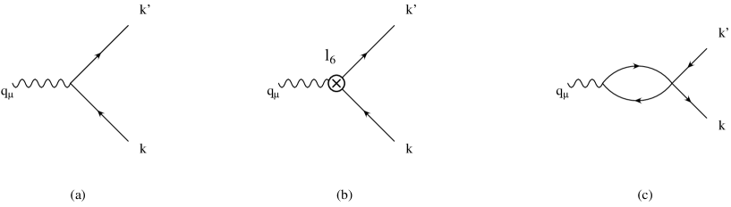
Figure 3:

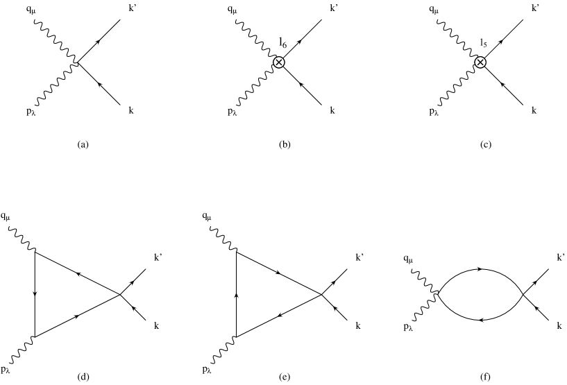
Figure 4:

Figure 5:

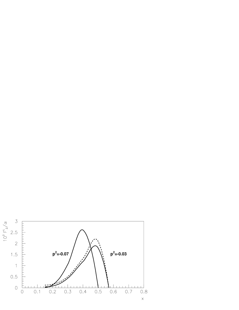
Figure 6:

Figure 7:

Figure 8:

References

- [1] A.S.Gorsky, B.L.Ioffe, A.Yu.Khodjamirian Phys. Lett. B227(1989) 474
- [2] A.Gorsky, B.Ioffe, A.Khodjamirian, A.Oganesian Z.Phys. C44(1989) 523
- [3] A.Smilga Comm. Nucl. Part. Phys. 20(1991) 69
- [4] H.F. Contopanagos, M.B. Einhorn Phys.Rev. D45(1992) 1291, 1322, Nucl.Phys. B377(1992) 20
- [5] B. Ioffe, A. Oganesian Z. Phys. C69(1995) 119
- [6] J.Gasser, H.Leutwyler Ann. Phys. 158(1984) 142
- [7] Ulf-G.Meissner Rep. Prog. Phys. 56(1993) 903
- [8] H.Leutwyler Ann. Phys. 235(1994) 165
- [9] B.L. Ioffe, V.A. Khoze, L.N.Lipatov Hard Processes, North Holland, Amsterdam, 1984